Using lumi, a package processing Illumina Microarray · Using lumi, a package processing Illumina Microarray Pan Duz, Gang Fengzy, Warren A. Kibbezz, Simon Linzx July 4, 2015 zRobert

Using lumi, a package processing Illumina

Microarray

Pan Du‡∗, Gang Feng‡†, Warren A. Kibbe‡‡, Simon Lin‡§

July 4, 2015

‡Robert H. Lurie Comprehensive Cancer CenterNorthwestern University, Chicago, IL, 60611, USA

Contents

1 Overview of lumi 2

2 Citation 2

3 Installation of lumi package 3

4 Object models of major classes 3

5 Data preprocessing 35.1 Intelligently read the BeadStudio output file . . . . . . . . . . . . 55.2 Quality control of the raw data . . . . . . . . . . . . . . . . . . . 85.3 Background correction . . . . . . . . . . . . . . . . . . . . . . . . 185.4 Variance stabilizing transform . . . . . . . . . . . . . . . . . . . . 195.5 Data normalization . . . . . . . . . . . . . . . . . . . . . . . . . . 195.6 Quality control after normalization . . . . . . . . . . . . . . . . . 235.7 Encapsulate the processing steps . . . . . . . . . . . . . . . . . . 235.8 Inverse VST transform to the raw scale . . . . . . . . . . . . . . 30

6 Handling large data sets 32

7 Performance comparison 33

8 Gene annotation 33

9 A use case: from raw data to functional analysis 349.1 Preprocess the Illumina data . . . . . . . . . . . . . . . . . . . . 349.2 Identify differentially expressed genes . . . . . . . . . . . . . . . . 359.3 Gene Ontology and other functional analysis . . . . . . . . . . . 379.4 GEO submission of the data . . . . . . . . . . . . . . . . . . . . . 38∗dupan.mail (at) gmail.com†g-feng (at) northwestern.edu‡wakibbe (at) northwestern.edu§s-lin2 (at) northwestern.edu

1

10 Session Info 39

11 Acknowledgments 39

12 References 40

1 Overview of lumi

Illumina microarray is becoming a popular microarray platform. The BeadArraytechnology from Illumina makes its preprocessing and quality control differentfrom other microarray technologies. Unfortunately, until now, most analyseshave not taken advantage of the unique properties of the BeadArray system.The lumi Bioconductor package especially designed to process the Illumina mi-croarray data, including Illumina Expression and Methylation microarray data.The lumi package provides an integrated solution for the bead-level Illumina mi-croarray data analysis. The package covers data input, quality control, variancestabilization, normalization and gene annotation.

For details of processing Illumina methylation microarray, especially In-finium methylation microarray, please check another tutorial in lumi package:”Analyze Illumina Infinium methylation microarray data”. All following descrip-tion is focused on processing Illumina expression microarrays.

The lumi package provides unique functions for expression microarray pro-cessing. It includes a variance-stabilizing transformation (VST) algorithm [2]that takes advantage of the technical replicates available on every Illumina mi-croarray. A robust spline normalization (RSN), which combines the features ofthe quantile and loess normalization, and simple scaling normalization (SSN)algorithms are also implemented in this package. Options available in other pop-ular normalization methods are also provided. Multiple quality control plots forexpression and control probe data are provided in the package. To better anno-tate the Illumina data, a new, vendor independent nucleotide universal identifier(nuID) [3] was devised to identify the probes of Illumina microarray. The nuIDindexed Illumina annotation packages is compatible with other Bioconductor an-notation packages. Mappings from Illumina Target Id or Probe Id to nuID arealso included in the annotation packages. The output of lumi processed resultscan be easily integrated with other microarray data analysis, like differentiallyexpressed gene identification, gene ontology analysis or clustering analysis.

2 Citation

For the people using lumi package, please cite the following papers in yourpublications.

* For the package:Du, P., Kibbe, W.A. and Lin, S.M., (2008) ’lumi: a pipeline for processing

Illumina microarray’, Bioinformatics 24(13):1547-1548* For the VST (variance stabilization transformation) algorithm, please cite:Lin, S.M., Du, P., Kibbe, W.A., (2008) ’Model-based Variance-stabilizing

Transformation for Illumina Microarray Data’, Nucleic Acids Res. 36, e11* For nuID annotation packages, please cite:

2

Du, P., Kibbe, W.A. and Lin, S.M., (2007) ’nuID: A universal naming schemaof oligonucleotides for Illumina, Affymetrix, and other microarrays’, BiologyDirect, 2, 16.

Thanks for your help!

3 Installation of lumi package

In order to install the lumi package, the user needs to first install R, some relatedBioconductor packages. You can easily install them by the following codes.

source("http://bioconductor.org/biocLite.R")

biocLite("lumi")

For the users want to install the latest developing version of lumi, whichcan be downloaded from the developing section of Bioconductor website. Someadditional packages may be required to be installed because of the update theBioconductor. These packages can also be found from the developing sectionof Bioconductor website. You can also directly install the source packages fromthe Bioconductor website by specify the developing version number, which canbe found at the Bioconductor website. Suppose the developing version is 2.3, toinstall the latest lumi pakcage in the Bioconductor developing version, you canuse the following command:

## replace "xxx" with the Bioconductor version number.

install.packages("lumi",repos="http://www.bioconductor.org/packages/xxx/bioc",type="source")

An Illumina benchmark data package lumiBarnes can be downloaded fromBioconductor Experiment data website.

4 Object models of major classes

The lumi package has one major class: LumiBatch. LumiBatch is inheritedfrom ExpressionSet class in Bioconductor for better compatibility. Their re-lations are shown in Figure 1. LumiBatch class includes se.exprs, beadNumand detection in assayData slot for additional informations unique to Illuminamicroarrays. A controlData slot is used to keep the control probe information,and a QC slot is added for keeping the quality control information. The S4 func-tion plot supports different kinds of plots by specifying the specific plot type ofLumiBatch object. See help of plot-methods function for details. The historyslot records all the operations made on the LumiBatch object. This providesdata provenance. Function getHistory is to retrieve the history slot. Pleasesee the help files of LumiBatch class for more details. A series of functions:lumiR, lumiR.batch, lumiB, lumiT, lumiN and lumiQ were designed for datainput, preprocessing and quality control. Function lumiExpresso encapsulatesthe preprocessing methods for easier usability.

5 Data preprocessing

The first thing is to load the lumi package.

> library(lumi)

3

Figure 1: Object models in lumi package

4

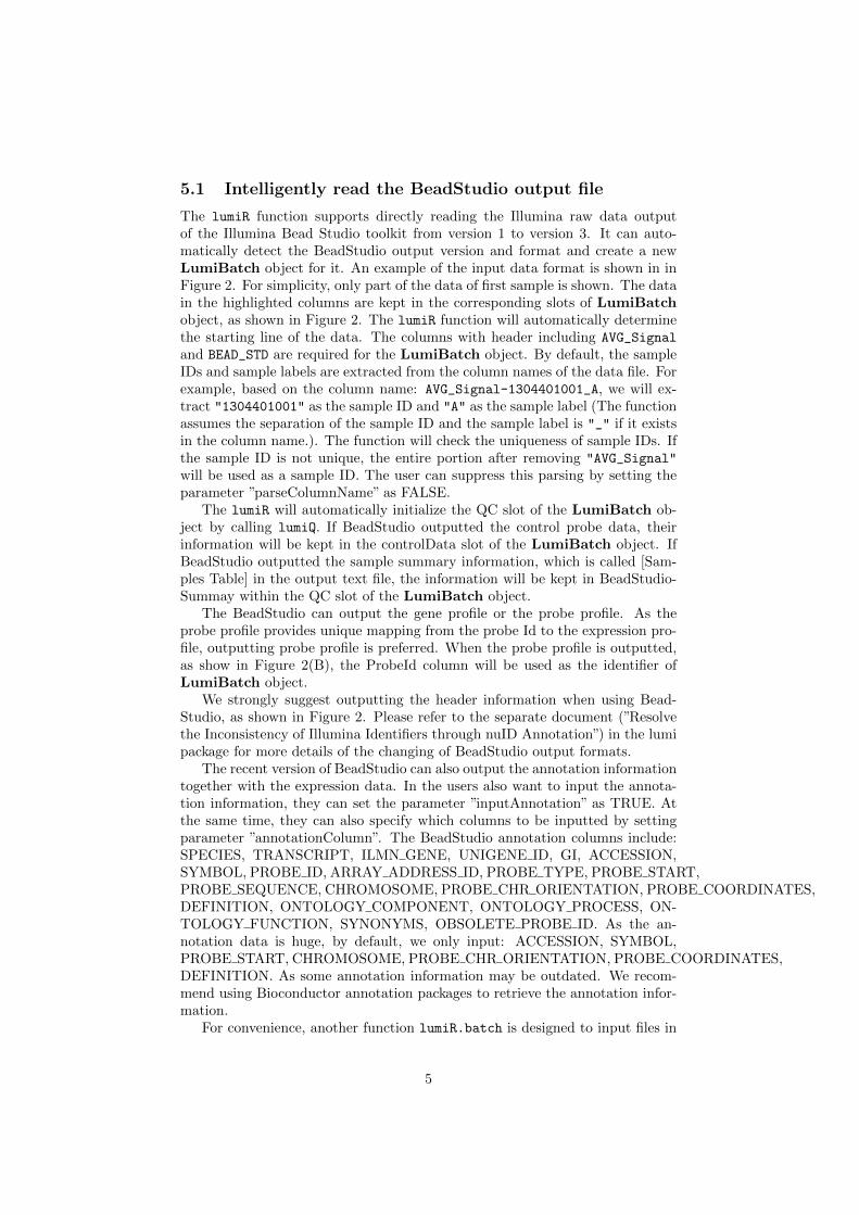
5.1 Intelligently read the BeadStudio output file

The lumiR function supports directly reading the Illumina raw data outputof the Illumina Bead Studio toolkit from version 1 to version 3. It can auto-matically detect the BeadStudio output version and format and create a newLumiBatch object for it. An example of the input data format is shown in inFigure 2. For simplicity, only part of the data of first sample is shown. The datain the highlighted columns are kept in the corresponding slots of LumiBatchobject, as shown in Figure 2. The lumiR function will automatically determinethe starting line of the data. The columns with header including AVG_Signal

and BEAD_STD are required for the LumiBatch object. By default, the sampleIDs and sample labels are extracted from the column names of the data file. Forexample, based on the column name: AVG_Signal-1304401001_A, we will ex-tract "1304401001" as the sample ID and "A" as the sample label (The functionassumes the separation of the sample ID and the sample label is "_" if it existsin the column name.). The function will check the uniqueness of sample IDs. Ifthe sample ID is not unique, the entire portion after removing "AVG_Signal"

will be used as a sample ID. The user can suppress this parsing by setting theparameter ”parseColumnName” as FALSE.

The lumiR will automatically initialize the QC slot of the LumiBatch ob-ject by calling lumiQ. If BeadStudio outputted the control probe data, theirinformation will be kept in the controlData slot of the LumiBatch object. IfBeadStudio outputted the sample summary information, which is called [Sam-ples Table] in the output text file, the information will be kept in BeadStudio-Summay within the QC slot of the LumiBatch object.

The BeadStudio can output the gene profile or the probe profile. As theprobe profile provides unique mapping from the probe Id to the expression pro-file, outputting probe profile is preferred. When the probe profile is outputted,as show in Figure 2(B), the ProbeId column will be used as the identifier ofLumiBatch object.

We strongly suggest outputting the header information when using Bead-Studio, as shown in Figure 2. Please refer to the separate document (”Resolvethe Inconsistency of Illumina Identifiers through nuID Annotation”) in the lumipackage for more details of the changing of BeadStudio output formats.

The recent version of BeadStudio can also output the annotation informationtogether with the expression data. In the users also want to input the annota-tion information, they can set the parameter ”inputAnnotation” as TRUE. Atthe same time, they can also specify which columns to be inputted by settingparameter ”annotationColumn”. The BeadStudio annotation columns include:SPECIES, TRANSCRIPT, ILMN GENE, UNIGENE ID, GI, ACCESSION,SYMBOL, PROBE ID, ARRAY ADDRESS ID, PROBE TYPE, PROBE START,PROBE SEQUENCE, CHROMOSOME, PROBE CHR ORIENTATION, PROBE COORDINATES,DEFINITION, ONTOLOGY COMPONENT, ONTOLOGY PROCESS, ON-TOLOGY FUNCTION, SYNONYMS, OBSOLETE PROBE ID. As the an-notation data is huge, by default, we only input: ACCESSION, SYMBOL,PROBE START, CHROMOSOME, PROBE CHR ORIENTATION, PROBE COORDINATES,DEFINITION. As some annotation information may be outdated. We recom-mend using Bioconductor annotation packages to retrieve the annotation infor-mation.

For convenience, another function lumiR.batch is designed to input files in

5

Figure 2: An example of the input data format

6

batch. Basically it combines the output of each file. See the help of lumiR.batchfor details. lumiR.batch function also allows users to add sample informationin the phenoData slot of the LumiBatch object. This will be useful in the dataanalysis. The sampleInfoFile parameter is optional. The file is a Tab-separatedtext file. The first ID column is required. It represents sample ID, which is de-fined based on the column names of BeadStudio output file. For example, sampleID of column ”1881436070 A STA.AVG Signal” is ”1881436070 A STA”. Thesample ID column can also be found in the ”Samples Table.txt” file output byBeadStudio. Another ”Label” column (if provided) will be used as the sample-Names of LumiBatch object. All information of sampleInfoFile will be directlyadded in the phenoData slot in LumiBatch object, which can be retrieved bythe command like: pData(phenoData(x.lumi)).

> ## specify the file name

> # fileName <- 'Barnes_gene_profile.txt'

> ## load the data

> # x.lumi <- lumiR.batch(fileName, sampleInfoFile='sampleInfo.txt') # Not Run

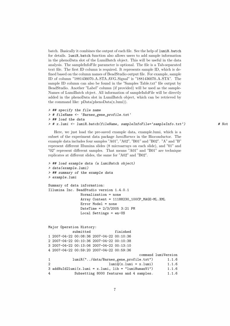
Here, we just load the pre-saved example data, example.lumi, which is asubset of the experiment data package lumiBarnes in the Bioconductor. Theexample data includes four samples ”A01”, ”A02”, ”B01” and ”B02”. ”A” and ”B”represent different Illumina slides (8 microarrays on each slide), and ”01” and”02” represent different samples. That means ”A01” and ”B01” are techniquereplicates at different slides, the same for ”A02” and ”B02”.

> ## load example data (a LumiBatch object)

> data(example.lumi)

> ## summary of the example data

> example.lumi

Summary of data information:

Illumina Inc. BeadStudio version 1.4.0.1

Normalization = none

Array Content = 11188230_100CP_MAGE-ML.XML

Error Model = none

DateTime = 2/3/2005 3:21 PM

Local Settings = en-US

Major Operation History:

submitted finished

1 2007-04-22 00:08:36 2007-04-22 00:10:36

2 2007-04-22 00:10:36 2007-04-22 00:10:38

3 2007-04-22 00:13:06 2007-04-22 00:13:10

4 2007-04-22 00:59:20 2007-04-22 00:59:36

command lumiVersion

1 lumiR("../data/Barnes_gene_profile.txt") 1.1.6

2 lumiQ(x.lumi = x.lumi) 1.1.6

3 addNuId2lumi(x.lumi = x.lumi, lib = "lumiHumanV1") 1.1.6

4 Subsetting 8000 features and 4 samples. 1.1.6

7

Object Information:

LumiBatch (storageMode: lockedEnvironment)

assayData: 8000 features, 4 samples

element names: beadNum, detection, exprs, se.exprs

protocolData: none

phenoData

sampleNames: A01 A02 B01 B02

varLabels: sampleID label

varMetadata: labelDescription

featureData

featureNames: oZsQEQXp9ccVIlwoQo 9qedFRd_5Cul.ueZeQ ...

33KnLHy.RFaieogAF4 (8000 total)

fvarLabels: TargetID

fvarMetadata: labelDescription

experimentData: use 'experimentData(object)'

Annotation: lumiHumanAll.db

Control Data: Available

QC information: Please run summary(x, 'QC') for details!

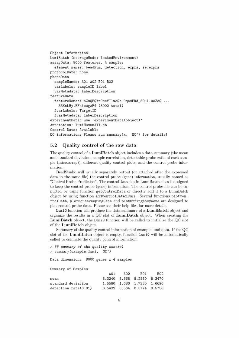
5.2 Quality control of the raw data

The quality control of a LumiBatch object includes a data summary (the meanand standard deviation, sample correlation, detectable probe ratio of each sam-ple (microarray)), different quality control plots, and the control probe infor-mation.

BeadStudio will usually separately output (or attached after the expresseddata in the same file) the control probe (gene) information, usually named as”Control Probe Profile.txt”. The controlData slot in LumiBatch class is designedto keep the control probe (gene) information. The control probe file can be in-putted by using function getControlData or directly add it to a LumiBatchobject by using function addControlData2lumi. Several functions plotCon-

trolData, plotHousekeepingGene and plotStringencyGene are designed toplot control probe data. Please see their help files for more details.

LumiQ function will produce the data summary of a LumiBatch object andorganize the results in a QC slot of LumiBatch object. When creating theLumiBatch object, the LumiQ function will be called to initialize the QC slotof the LumiBatch object.

Summary of the quality control information of example.lumi data. If the QCslot of the LumiBatch object is empty, function lumiQ will be automaticallycalled to estimate the quality control information.

> ## summary of the quality control

> summary(example.lumi, 'QC')

Data dimension: 8000 genes x 4 samples

Summary of Samples:

A01 A02 B01 B02

mean 8.3240 8.568 8.2580 8.3470

standard deviation 1.5580 1.686 1.7230 1.6690

detection rate(0.01) 0.5432 0.564 0.5774 0.5758

8

distance to sample mean 76.9500 65.280 88.3200 49.1100


submitted finished

1 2007-04-22 00:08:36 2007-04-22 00:10:36

2 2007-04-22 00:10:36 2007-04-22 00:10:38

command lumiVersion



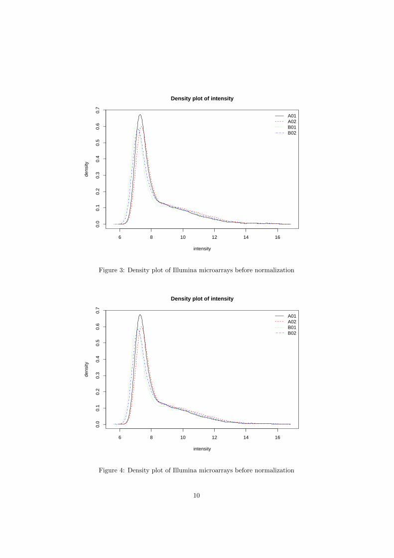
The S4 method plot can produce the quality control plots of LumiBatchobject. The quality control plots includes: the density plot (Figure 4), box plot(Figure ??), pairwise scatter plot between microarrays (Figure 6) or pair scatterplot with smoothing (Figure 7), pairwise MAplot between microarrays (Figure8) or MAplot with smoothing (Figure 9), density plot of coefficient of varience,(Figure 10), and the sample relations (Figure 11). More details are in the helpof plot,LumiBatch-method function. Most of these plots can also be plotted bythe extended general functions: density (for density plot), boxplot, MAplot,pairs and plotSampleRelation.

Figure 4 shows the density plot of the LumiBatch object by using plot ordensity functions.

> ## plot the density

> plot(example.lumi, what='density')

> ## or

> density(example.lumi)

Figure 4 shows the density plot of the LumiBatch object by using plot ordensity functions.

> ## plot the density

> plot(example.lumi, what='density')

> ## or

> density(example.lumi)

Figure 5 shows the plot of Cumulative Distribution Function (CDF) fromhigh to low value or in reverse of a LumiBatch object by using plotCDF func-tion. Comparing with the density plot, the CDF plot in reverse direction canbetter show the different at the high and middle expression range among differ-ent samples.

> ## plot the CDF plot

> plotCDF(example.lumi, reverse=TRUE)

Figure 6 shows the pairwise sample correlation of the LumiBatch objectby using plot or pairs functions.

> ## plot the pair plot

> plot(example.lumi, what='pair')

> ## or

> pairs(example.lumi)

> ## pairwise scatter plot with smoothing

> pairs(example.lumi, smoothScatter=T)

9

6 8 10 12 14 16

0.0

0.1

0.2

0.3

0.4

0.5

0.6

0.7

Density plot of intensity

intensity

dens

ity

A01A02B01B02

Figure 3: Density plot of Illumina microarrays before normalization

6 8 10 12 14 16

0.0

0.1

0.2

0.3

0.4

0.5

0.6

0.7


intensity

dens

ity

A01A02B01B02

Figure 4: Density plot of Illumina microarrays before normalization

10

log2 intensity

Cum

ulat

ive

dens

ity

16 14 12 10 8 6

0.0

0.2

0.4

0.6

0.8

1.0

A01A02B01B02

Figure 5: Cumulative Distribution Function (CDF) plot of Illumina microarraysbefore normalization

11

A01

8 10 12 14 16 6 8 10 12 14 16

810

1214

16

810

1214

16

Cor = 0.965 0 (> 2, up)

209 (> 2, down)

A02

Cor = 0.992 3 (> 2, up)

0 (> 2, down)

Cor = 0.965 234 (> 2, up)0 (> 2, down)

B01

68

1012

1416

8 10 12 14 16

68

1012

1416

Cor = 0.964 0 (> 2, up)

158 (> 2, down)

Cor = 0.993 12 (> 2, up)

1 (> 2, down)

6 8 10 12 14 16

Cor = 0.964 1 (> 2, up)

178 (> 2, down)

B02

Pairwise plot with sample correlation

Figure 6: Pairwise plot with microarray correlation before normalization

12

A01

8 10 12 14 16

8 10 12 14 16

810

1214

16

x[subset]

y[su

bset

]

6 8 10 12 14 16

810

1214

16

x[subset]

y[su

bset

]

6 8 10 12 14 16

810

1214

16

6 8 10 12 14 16

810

1214

16x[subset]

y[su

bset

]

810

1214

16

Cor = 0.965 0 (> 2, up)

209 (> 2, down)

A02

6 8 10 12 14 16

810

1214

16

x[subset]

y[su

bset

]

6 8 10 12 14 16

810

1214

16

x[subset]

y[su

bset

]

Cor = 0.992 3 (> 2, up)

0 (> 2, down)

Cor = 0.965 234 (> 2, up)0 (> 2, down)

B01

68

1012

1416

6 8 10 12 14 16

68

1012

1416

x[subset]

y[su

bset

]

8 10 12 14 16

68

1012

1416

Cor = 0.964 0 (> 2, up)

158 (> 2, down)

Cor = 0.993 12 (> 2, up)

1 (> 2, down)

6 8 10 12 14 16

Cor = 0.964 1 (> 2, up)

178 (> 2, down)

B02


Figure 7: Pairwise plot with microarray correlation before normalization

13

A01

8 10 12 14 16−

6−

4−

20

Median: −0.189IQR: 0.342

8 10 12 14 16−1.

00.

01.

02.

0

Median: 0.0733IQR: 0.396

8 10 12 14 16

−6

−4

−2

0

Median: 0.0196IQR: 0.321

A02

8 10 12 14 160

24

68

Median: 0.244IQR: 0.293

8 10 12 14 16

−1.

00.

00.

51.

0

Median: 0.22IQR: 0.242

B01

8 10 12 14 16−

8−

6−

4−

20

Median: −0.0327IQR: 0.32

B02

A

M

Pairwise MA plots between samples

Figure 8: Pairwise MAplot before normalization

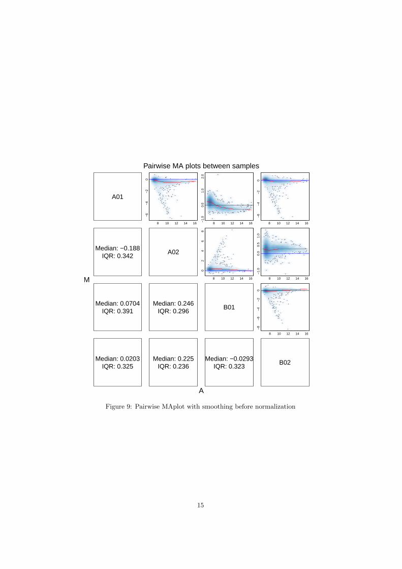
Figure 8 shows the MA plot of the LumiBatch object by using plot orMAplot functions.

> ## plot the MAplot

> plot(example.lumi, what='MAplot')

> ## or

> MAplot(example.lumi)

> ## with smoothing

> MAplot(example.lumi, smoothScatter=TRUE)

The density plot of the coefficient of variance of the LumiBatch object. SeeFigure 10. Figure 10 shows the density plot of the coefficient of variance of theLumiBatch object by using plot function.

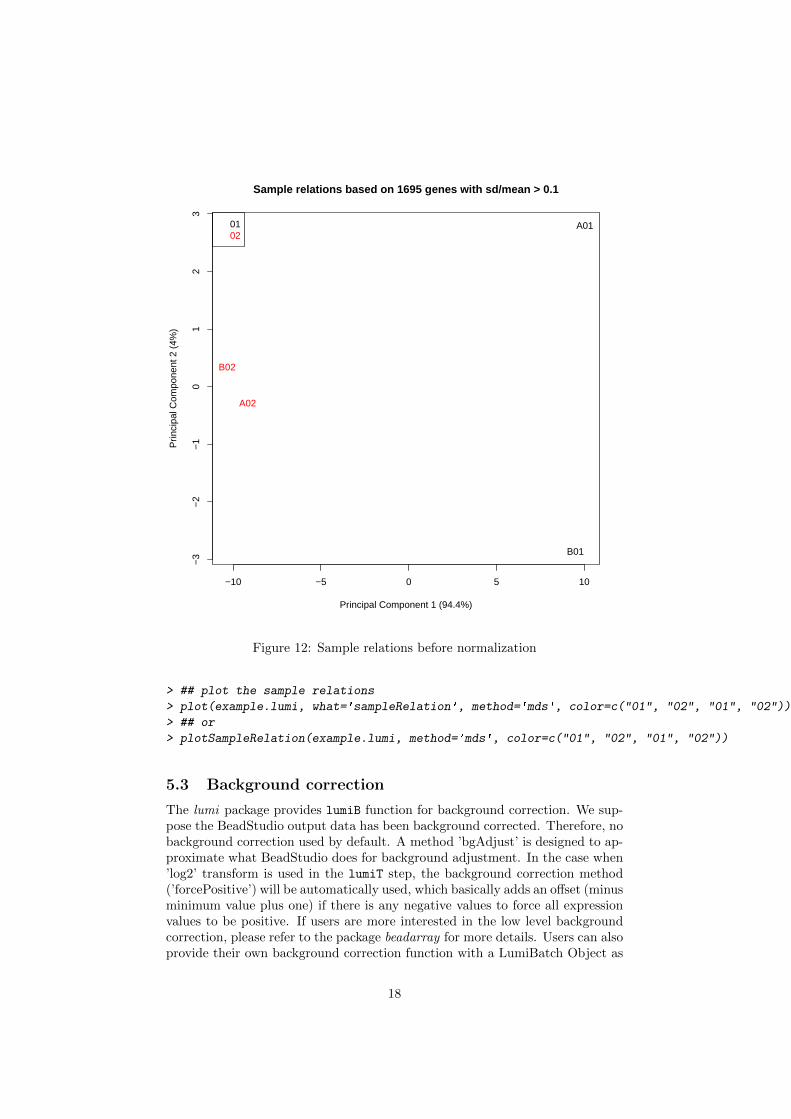
Figure 11 shows the sample relations using hierarchical clustering.Figure 12 shows the sampleRelation using MDS. The color of the sample is

based on the sample type, which is "01", "02", "01", "02" for the sampledata. Please see the help of plotSampleRelation and plot-methods for moredetails.

14

A01

8 10 12 14 16

−6

−4

−2

0

Median: −0.188IQR: 0.342

8 10 12 14 16−1.

00.

01.

02.

0

Median: 0.0704IQR: 0.391

8 10 12 14 16

−6

−4

−2

0

Median: 0.0203IQR: 0.325

A02

8 10 12 14 16

02

46

8

Median: 0.246IQR: 0.296

8 10 12 14 16

−1.

00.

00.

51.

0

Median: 0.225IQR: 0.236

B01

8 10 12 14 16

−8

−6

−4

−2

0

Median: −0.0293IQR: 0.323

B02

A

M


Figure 9: Pairwise MAplot with smoothing before normalization

15

> ## density plot of coefficient of varience

> plot(example.lumi, what='cv')

−8 −7 −6 −5 −4 −3 −2

0.0

0.1

0.2

0.3

0.4

0.5

0.6

0.7

Density plot of coefficient of variance

coefficient of variance (log2)

Den

sity

A01A02B01B02

Figure 10: Density Plot of Coefficient of Varience

16

> plot(example.lumi, what='sampleRelation')

A02

B02

A01

B01

510

1520

Sample relations based on 1695 genes with sd/mean > 0.1

hclust (*, "average")Sample

Hei

ght

Figure 11: Sample relations before normalization

17

−10 −5 0 5 10

−3

−2

−1

01

23


Principal Component 1 (94.4%)

Prin

cipa

l Com

pone

nt 2

(4%

)

A01

A02

B01

B02

0102

Figure 12: Sample relations before normalization

> ## plot the sample relations

> plot(example.lumi, what='sampleRelation', method='mds', color=c("01", "02", "01", "02"))

> ## or

> plotSampleRelation(example.lumi, method='mds', color=c("01", "02", "01", "02"))

5.3 Background correction

The lumi package provides lumiB function for background correction. We sup-pose the BeadStudio output data has been background corrected. Therefore, nobackground correction used by default. A method ’bgAdjust’ is designed to ap-proximate what BeadStudio does for background adjustment. In the case when’log2’ transform is used in the lumiT step, the background correction method(’forcePositive’) will be automatically used, which basically adds an offset (minusminimum value plus one) if there is any negative values to force all expressionvalues to be positive. If users are more interested in the low level backgroundcorrection, please refer to the package beadarray for more details. Users can alsoprovide their own background correction function with a LumiBatch Object as

18

the first argument and return a LumiBatch Object with background corrected.See lumiB help document for more details.

5.4 Variance stabilizing transform

Variance stabilization is critical for subsequent statistical inference to identifydifferential genes from microarray data. We devised a variance-stabilizing trans-formation (VST) by taking advantages of larger number of technical replicatesavailable on the Illumina microarray. Please see [2] for details of the algorithm.

Because the STDEV (or STDERR) columns of the BeadStudio output fileis the standard error of the mean of the bead intensities corresponding to thesame probe. (Thanks Gordon Smyth kindly provided this information!). Asthe variance stabilization (see help of vst function) requires the informationof the standard deviation instead of the standard error of the mean, the valuecorrection is required. The corrected value will be x * sqrt(N), where x is theold value (standard error of the mean), N is the number of beads correspondingto the probe. The parameter ’stdCorrection’ of lumiT determines whether todo this conversion and is effective only when the ’vst’ method is selected. Bydefault, the parameter ’stdCorrection’ is TRUE.

Function lumiT performs variance stabilizing transform with both input andoutput being LumiBatch object.

Do default VST variance stabilizing transform

> ## Do default VST variance stabilizing transform

> lumi.T <- lumiT(example.lumi)

Perform vst transformation ...

2015-07-04 18:45:29 , processing array 1




The plotVST can plot the transformation function of VST, see Figure 13,which is close to log2 at high expression values, see Figure 14. Function lumiT

also provides options to do "log2" or "cubicRoot" transform. See help oflumiT for details.

> ## plot VST transformation

> trans <- plotVST(lumi.T)

> ## compare the log2 and VST transform

> matplot(log2(trans$untransformed), trans$transformed, main='compare VST and log2 transform', xlab='log2 transformed', ylab='vST transformed')

5.5 Data normalization

lumi package provides several normalization method options, which includequantile, SSN (Simple Scaling Normalization), RSN (Robust Spline Normal-ization), loess normalization and Rank Invariant Normalization.

Comparing with other normalization methods, like quantile and curve-fittingmethods, SSN is a more conservative method. The only assumption is that eachsample has the same background level and the same scale (if do scaling). It ba-sically make all the samples have the same background level and the same scale

19

0 20000 40000 60000 80000

810

1214

16

un−transformed value

tran

sfor

med

val

ue

A01A02B01B02

Figure 13: VST transformation

20

8 10 12 14 16

810

1214

16

compare VST and log2 transform

log2 transformed

vST

tran

sfor

med

Figure 14: Compare VST and log2 transform

21

comparing to the background (if do scaling). There are three methods (’density’,’mean’ and ’median’) for background estimation. If bgMethod is ’none’, thenno background adjustment. For the ’density’ bgMethod, it estimates the back-ground based on the mode of probe intensities based on the assumption thatthe background level intensity is the most frequent value across all the probesin the chip. For the foreground level estimation, it also provides three meth-ods (’mean’, ’density’, ’median’). For the ’density’ fgMethod, it assumes thebackground probe levels are symmetrically distributed. The foreground levelswere estimated by taking the intensity mean of all other probes except from thebackground probes. For the ’mean’ and ’median’ methods (for both bgMethodand fgMethod), it basically estimates the level based on the mean or medianof all probes of the sample. If the fgMethod is the same as bgMethod (except’density’ method), no scaling will be performed.

Another normalization method which is unique in the lumi package is theRobust Spline Normalization (RSN) algorithm. RSN combines the features ofquanitle and loess nor-malization. The advantages of quantile normalization in-clude computational efficiency and preserving the rank order of genes. However,the intensity transformation of a quantile normalization is discontinuous becausethe normalization forces the intensity values for different samples (microarrrays)having exactly the same distribution. This can cause small differences amongintensity values to be lost. In contrast, the loess or spline normalization pro-vides a continuous transformation. However, these methods cannot ensure thatthe rank of the probes remain unchanged across samples. Moreover, the loessnormalization assumes the majority of the genes measured by the probes arenon-differentially expressed and their distribution is approximately symmetric,which may not be a good assumption. To address some of these concerns, we de-veloped a Robust Spline Normalization (RSN) method, which combines featuresfrom loess and quantile normalization methods. We use a monotonic spline tocalibrate one microarray to the reference microarray. To increase the robustnessof the spline method, we down-weight the contributions of probes of putativelydifferentially expressed genes. The probe intensities that are from potentiallydifferentially expressed genes are heuristically determined as follows: First, werun a quantile normalization. Next, we estimate the fold-change of a gene mea-sured by a probe based on the quantile-normalized data. The weighting factorfor a probe is calculated based on a Gaussian window function. More detailswill be shown in a separate manuscript.

The default normalization method used in the Illumina BeadStudio softwareis Rank Invariant Normalization. In order to support similar functionalities, thelumi package also provides a similar normalization implementation call ”rankin-variant” (We thanks Arno Velds implemented this function.). Please check thehelp of rankinvariant for more details.

By default, function lumiN performs popular quantile normalization. lumiNalso provides other options to do "rsn", "ssn", "loess", "vsn", "rankin-

variant" normalization. See help of lumiN for details.Do default quantile between microarray normaliazation

> ## Do quantile between microarray normaliazation

> lumi.N <- lumiN(lumi.T)

Perform quantile normalization ...

22

Users can also easily select other normalization method. For example, thefollowing command will run RSN normalization.

> ## Do RSN between microarray normaliazation

> lumi.N <- lumiN(lumi.T, method='rsn')

5.6 Quality control after normalization

To make sure the data quality meets our requirement, we do a second round ofquality control of normalized data with different QC plots. Compare the plotsbefore and after normalization, we can clearly see the improvements.

> ## Do quality control estimation after normalization

> lumi.N.Q <- lumiQ(lumi.N)

Perform Quality Control assessment of the LumiBatch object ...

> ## summary of the quality control

> summary(lumi.N.Q, 'QC') ## summary of QC

Data dimension: 8000 genes x 4 samples

Summary of Samples:

A01 A02 B01 B02

mean 8.8430 8.843 8.8430 8.8430

standard deviation 1.3350 1.335 1.3350 1.3350

detection rate(0.01) 0.5432 0.564 0.5774 0.5758

distance to sample mean 15.3300 15.080 15.3200 15.4500


submitted finished

1 2007-04-22 00:08:36 2007-04-22 00:10:36

2 2007-04-22 00:10:36 2007-04-22 00:10:38

3 2007-04-22 00:13:06 2007-04-22 00:13:10

4 2007-04-22 00:59:20 2007-04-22 00:59:36

5 2015-07-04 18:45:29 2015-07-04 18:45:29

6 2015-07-04 18:45:29 2015-07-04 18:45:29

7 2015-07-04 18:45:29 2015-07-04 18:45:29

command lumiVersion



3 addNuId2lumi(x.lumi = x.lumi, lib = "lumiHumanV1") 1.1.6

4 Subsetting 8000 features and 4 samples. 1.1.6

5 lumiT(x.lumi = example.lumi) 2.20.2

6 lumiN(x.lumi = lumi.T) 2.20.2

7 lumiQ(x.lumi = lumi.N) 2.20.2

5.7 Encapsulate the processing steps

The lumiExpresso function is to encapsulate the major functions of Illuminapreprocessing. It is organized in a similar way as the expresso function in affy

23

> plot(lumi.N.Q, what='density') ## plot the density

8 10 12 14 16

0.0

0.2

0.4

0.6

0.8

1.0

1.2


intensity

dens

ity

A01A02B01B02

Figure 15: Density plot of Illumina microarrays after normalization

24

> plot(lumi.N.Q, what='boxplot') ## box plot

> # boxplot(lumi.N.Q)

810

1214

16

Boxplot of microarray intensity

microarrays

inte

nsity

A01

A02

B01

B02

Figure 16: Density plot of Illumina microarrays after normalization

25

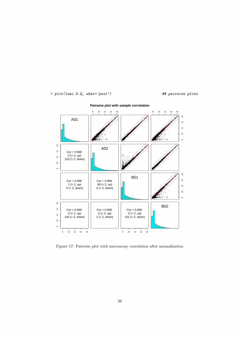
> plot(lumi.N.Q, what='pair') ## pairwise plots

A01

8 10 12 14 16 8 10 12 14 16

810

1214

16

810

1214

16

Cor = 0.969 0 (> 2, up)

103 (> 2, down)

A02

Cor = 0.996 1 (> 2, up)

0 (> 2, down)

Cor = 0.969 99 (> 2, up)

0 (> 2, down)

B018

1012

1416

8 10 12 14 16

810

1214

16

Cor = 0.969 0 (> 2, up)

104 (> 2, down)

Cor = 0.996 0 (> 2, up)

1 (> 2, down)

8 10 12 14 16

Cor = 0.969 0 (> 2, up)

101 (> 2, down)

B02


Figure 17: Pairwise plot with microarray correlation after normalization

26

> plot(lumi.N.Q, what='MAplot') ## plot the pairwise MAplot

A01

8 10 12 14 16

−6

−5

−4

−3

−2

−1

01

Median: 0.0318IQR: 0.173

8 10 12 14 16

−0.

50.

00.

51.

01.

5

Median: −0.00264IQR: 0.143

8 10 12 14 16

−6

−5

−4

−3

−2

−1

01

Median: 0.0307IQR: 0.18

A02

8 10 12 14 16

02

46

Median: −0.037IQR: 0.171

8 10 12 14 16

−1.

0−

0.5

0.0

0.5

Median: −0.000323IQR: 0.136

B01

8 10 12 14 16

−6

−4

−2

0

Median: 0.0327IQR: 0.17

B02

A

M


Figure 18: Pairwise MAplot after normalization

27

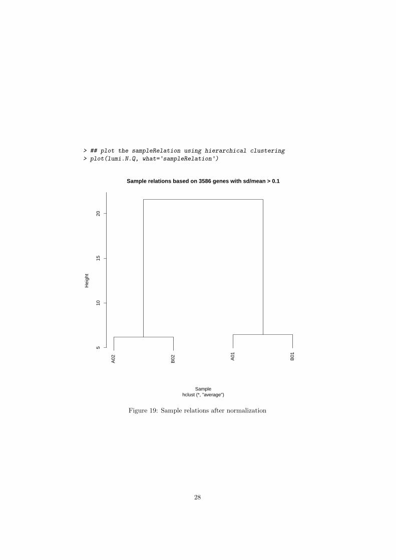
> ## plot the sampleRelation using hierarchical clustering

> plot(lumi.N.Q, what='sampleRelation')

A02

B02 A01

B01

510

1520


hclust (*, "average")Sample

Hei

ght

Figure 19: Sample relations after normalization

28

> ## plot the sampleRelation using MDS

> plot(lumi.N.Q, what='sampleRelation', method='mds', color=c("01", "02", "01", "02"))

−10 −5 0 5 10

−3

−2

−1

01

23


Principal Component 1 (91.7%)

Prin

cipa

l Com

pone

nt 2

(4.

4%)

A01

A02

B01

B02

0102

Figure 20: Sample relations after normalization

29

package. The following code basically did the same processing as the previousmulti-steps and produced the same results lumi.N.Q.

> ## Do all the default preprocessing in one step

> lumi.N.Q <- lumiExpresso(example.lumi)

Background Correction: bgAdjust

Variance Stabilizing Transform method: vst

Normalization method: quantile

Background correction ...

Perform bgAdjust background correction ...

done.

Variance stabilizing ...

Perform vst transformation ...





done.

Normalizing ...

Perform quantile normalization ...

done.

Quality control after preprocessing ...

Perform Quality Control assessment of the LumiBatch object ...

done.

Users can easily customize the processing parameters. For example, if theuser wants to do ”rsn” normalization, the user can run the following code. Formore details, please read the help document of lumiExpresso function.

> ## Do all the preprocessing with customized settings

> # lumi.N.Q <- lumiExpresso(example.lumi, normalize.param=list(method='rsn'))

5.8 Inverse VST transform to the raw scale

Figure 14 shows VST is very close to log2 in the high expression range. Inconvenience, users usually can directly use 2^x to approximate the data in rawscale and estimate the fold-change. For the users concern more in the lowexpression range, we also provide the function inverseVST to resume the data inthe raw scale. Need to mention, the inverse transform should be performed afterstatistical analysis, or else it makes no sense to transform back and forth. TheinverseVST function can directly applied to the LumiBatch object after lumiTwith VST transform, or VST transform plus RSN normalization (default methodof lumiN). For the RSN normalized data, the inverse transform is based on theparameters of the Target Array because the Target Array is the benchmarkdata and is not changed after normalization. Other normalization methods, like

30

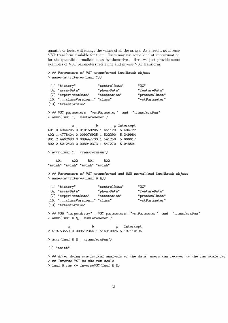
quantile or loess, will change the values of all the arrays. As a result, no inverseVST transform available for them. Users may use some kind of approximationfor the quantile normalized data by themselves. Here we just provide someexamples of VST parameters retrieving and inverse VST transform.

> ## Parameters of VST transformed LumiBatch object

> names(attributes(lumi.T))

[1] "history" "controlData" "QC"

[4] "assayData" "phenoData" "featureData"

[7] "experimentData" "annotation" "protocolData"

[10] ".__classVersion__" "class" "vstParameter"

[13] "transformFun"

> ## VST parameters: "vstParameter" and "transformFun"

> attr(lumi.T, 'vstParameter')

a b g Intercept

A01 0.4944205 0.010158205 1.461128 5.484722

A02 1.4778404 0.009076935 1.502390 5.349984

B01 2.4462693 0.009447733 1.541250 5.006017

B02 2.5012403 0.008940373 1.547270 5.048591

> attr(lumi.T, 'transformFun')

A01 A02 B01 B02

"asinh" "asinh" "asinh" "asinh"

> ## Parameters of VST transformed and RSN normalized LumiBatch object

> names(attributes(lumi.N.Q))

[1] "history" "controlData" "QC"

[4] "assayData" "phenoData" "featureData"

[7] "experimentData" "annotation" "protocolData"

[10] ".__classVersion__" "class" "vstParameter"

[13] "transformFun"

> ## VSN "targetArray" , VST parameters: "vstParameter" and "transformFun"

> attr(lumi.N.Q, 'vstParameter')

a b g Intercept

2.419753559 0.009512344 1.514310826 5.197110136

> attr(lumi.N.Q, 'transformFun')

[1] "asinh"

> ## After doing statistical analysis of the data, users can recover to the raw scale for the fold-change estimation.

> ## Inverse VST to the raw scale

> lumi.N.raw <- inverseVST(lumi.N.Q)

31

6 Handling large data sets

Several users asked about processing large data set, e.g., over 100 samples. Di-rectly handling such big data set usually will cause ”out of memory” error inmost computers. In this case, when read the BeadStudio output file, we can ig-nore the ”beadNum”(related columns. The function lumiR provides a parametercalled ”columnNameGrepPattern”. we can set the string grep pattern of ”detec-tion”and ”beadNum”as NA. You can also ignore ”detection”columns. However,the ”detection” information is useful for the estimation of present count of eachprobe and used in the VST parameter estimation. To further save memory,you can suppress the input of annotation data by setting ”inputAnnotation” asFALSE.

Here is some example code:

## load the data with empty detection and beadNum slots, and without annotation information

> x.lumi <- lumiR("fileName.txt", columnNameGrepPattern=list(beadNum=NA), inputAnnotation=FALSE)

Usually, the large data set is composed of many small data files. In thiscase, the transformations, like log2 and vst, can be performed right after theinput of each data file and some information can be removed in the object aftertransformation. lumi provides the lumiR.batch function for this purpose.

Here is some example code:

## load the list of data files (a vector of file names)

## and do VST transformation for each file and combine the results.

> x.lumi <- lumiR.batch(fileList, transform='vst')

Another good news is that the normalization, like rsn and ssn in the lumipackage, can sequentially process the data and handle such large data set.

The solution can be like this:1. Read the data file by smaller batches (e.g. 10 or just one by one), and

then do the variance stabilization for each data batch using lumiR.batch orlumiR function.

2. Pick one sample as the target array for normalization and then using”RSN” or ”SSN” normalization method to normalize all batches of data usingthe same target array.

3. Combine the normalized data. (In order to save memory, the user canfirst remove those probes not expressed in all samples.)

In the rsn and ssn functions, there is a parameter called ”targetArray”,which is the model for other chips to normalize. It can be a column index, avector or a LumiBatch object with one sample. In our case, we need to useone LumiBatch object with one sample as the ”targetArray”. The selection ofthe target array is flexible. We suggest to choose the one most similar to themean of all samples. For convenience, we can also just select the first sampleas ”targetArray” (suppose it has no quality problem). The selected target arraywill also be used for all other data batches. Since different data batches use thesame target array as model, the results are comparable and can be combined!

Here is the example code:

## Read in the Batch ith data file, suppose named as "fileName.i.txt"

> x.lumi.i <- lumiR("fileName.i.txt")

## variance stabilization (using vst or log2 transform)

32

> x.lumiT.i <- lumiT(x.lumi.i)

## select the "targetArray"

## This target array will also be used for other batches of data.

## For convenience, here we just select the first sample as targetArray.

> targetArray <- x.lumiT.i[,1]

## Do RSN normalization

> x.lumiN.i <- lumiN(x.lumiT.i, method='rsn', targetArray=targetArray)

The normalized data batches can be combined by using function combine(x,

y).

7 Performance comparison

We have selected the Barnes data set [4], which is a series dilution of two tissuesat five different dilutions, to compare different preprocessing methods. In orderto better compare the algorithms, we selected the samples with the smallestdilution difference (the most challenging comparison), i.e., the samples with thedilution ratios of 100:0 and 95:5 (each condition has two technical replicates)for comparison. For the Barnes data set, because we do not know which of thesignals are coming from ’true’ differentially expressed genes, we cannot use anROC curve to compare the performance of different algorithms. Instead, weevaluated the methods based on the concordance of normalized intensity profileand real dilution profile of the selected probes. More detailed evaluations withother criteria and based on other data sets can by found in our paper [2].

Following Barnes et al. (2005)[4], we defined a concordant gene (really aconcordant probe) as a signal from a probe with a correlation coefficient largerthan 0.8 between the normalized intensity profile and the real dilution profile(five dilution ratios with two replicates at each dilution ratio). If a selecteddifferentially expressed probe is also a concordant one, it is more likely to be trulydifferentially expressed. Figure 21 shows the percentage of concordant probesamong the selected probes, which were selected by ranking the probes’ p-value(calculated based on limma package) from low to high. We can see the VSTtransformed data outperforms the Log2-transformed and VSN processed data.For the normalization methods, RSN and quantile normalization have similarperformance for the VST transformed data, and RSN outperforms quantile forthe Log transformed data.

Please see another vignette in the lumi package: "lumi_vST_evaluation.pdf"for more details of the evaluation of VST (Variance Stabilizing Transformation).

8 Gene annotation

One challenge of Illumina microarray is the inconsistency and changes of Illu-mina identifiers across versions, even across different releases. This makes theintegration of the Illumina data difficult. In order to resolve these problems, weinvented a nuID (nucleotide universal IDentifier) annotation system, released re-lated annotation packages and a website to provide identifier mapping and thelatest annotation. Please refer to the separate document (”Resolve the Incon-sistency of Illumina Identifiers through nuID Annotation”) in the lumi packagefor more details.

33

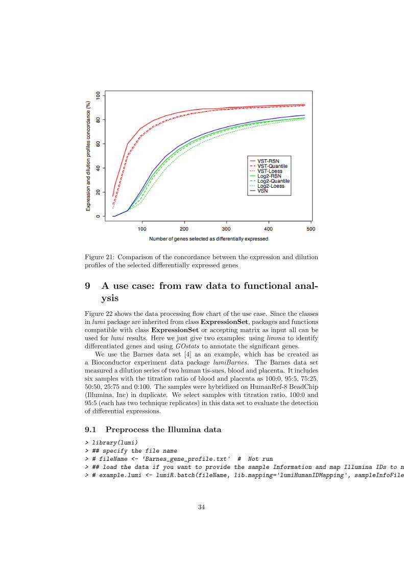
Figure 21: Comparison of the concordance between the expression and dilutionprofiles of the selected differentially expressed genes

9 A use case: from raw data to functional anal-ysis

Figure 22 shows the data processing flow chart of the use case. Since the classesin lumi package are inherited from class ExpressionSet, packages and functionscompatible with class ExpressionSet or accepting matrix as input all can beused for lumi results. Here we just give two examples: using limma to identifydifferentiated genes and using GOstats to annotate the significant genes.

We use the Barnes data set [4] as an example, which has be created asa Bioconductor experiment data package lumiBarnes. The Barnes data setmeasured a dilution series of two human tis-sues, blood and placenta. It includessix samples with the titration ratio of blood and placenta as 100:0, 95:5, 75:25,50:50, 25:75 and 0:100. The samples were hybridized on HumanRef-8 BeadChip(Illumina, Inc) in duplicate. We select samples with titration ratio, 100:0 and95:5 (each has two technique replicates) in this data set to evaluate the detectionof differential expressions.

9.1 Preprocess the Illumina data

> library(lumi)

> ## specify the file name

> # fileName <- 'Barnes_gene_profile.txt' # Not run

> ## load the data if you want to provide the sample Information and map Illumina IDs to nuIDs.

> # example.lumi <- lumiR.batch(fileName, lib.mapping='lumiHumanIDMapping', sampleInfoFile='sampleInfo.txt') # Not Run

34

Figure 22: Flow chart of the use case

> ## load saved data

> data(example.lumi)

> ## sumary of the daa

> example.lumi

> ## summary of quality control information

> summary(example.lumi, 'QC')

> ## preprocessing and quality control after normalization

> lumi.N.Q <- lumiExpresso(example.lumi, QC.evaluation=TRUE)

> ## summary of quality control information after preprocessing

> summary(lumi.N.Q, 'QC')

> ## Output the data as Tab separated text file

> write.exprs(lumi.N.Q, file='processedExampleData.txt')

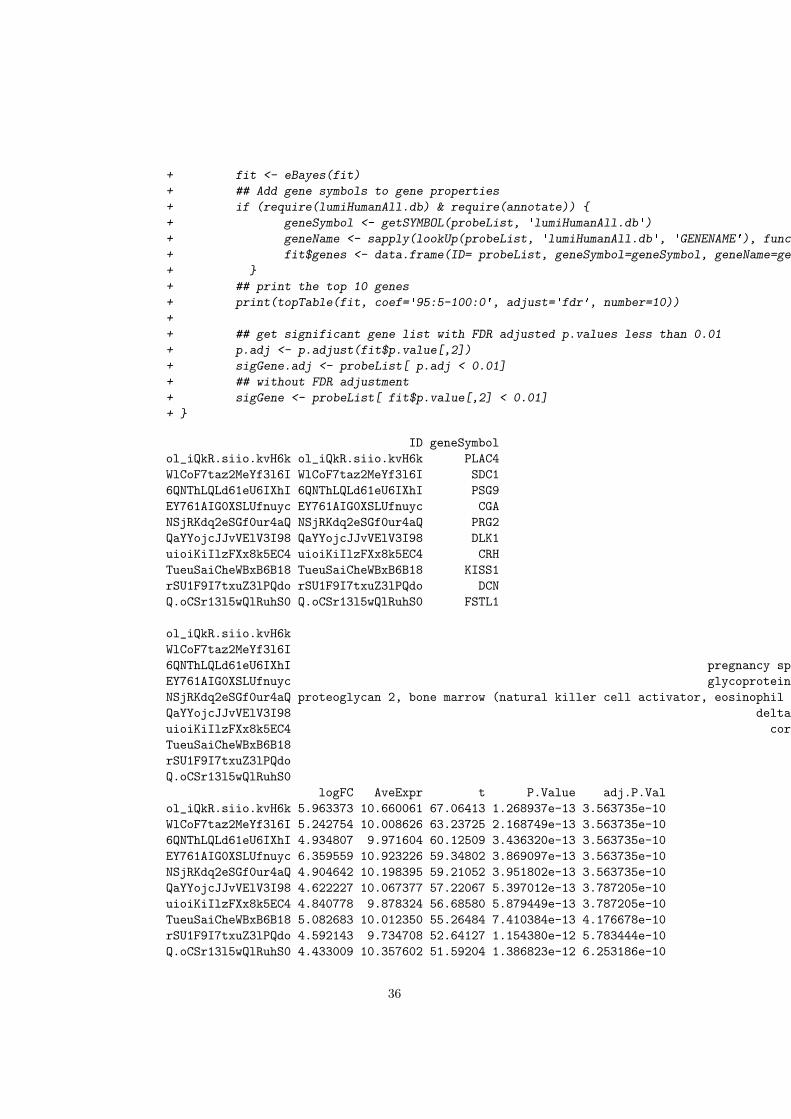
9.2 Identify differentially expressed genes

Identify the differentiated genes based on moderated t-test using limma.Retrieve the normalized data

> dataMatrix <- exprs(lumi.N.Q)

To speed up the processing and reduce false positives, remove the unex-pressed and un-annotated genes

> presentCount <- detectionCall(example.lumi)

> selDataMatrix <- dataMatrix[presentCount > 0,]

> if (require(lumiHumanAll.db) & require(annotate)) {

+ selDataMatrix <- selDataMatrix[!is.na(getSYMBOL(rownames(selDataMatrix), 'lumiHumanAll.db')),]

+ }

> probeList <- rownames(selDataMatrix)

> ## Specify the sample type

> sampleType <- c('100:0', '95:5', '100:0', '95:5')

> if (require(limma)) {

+ ## compare '95:5' and '100:0'

+ design <- model.matrix(~ factor(sampleType))

+ colnames(design) <- c('100:0', '95:5-100:0')

+ fit <- lmFit(selDataMatrix, design)

35

+ fit <- eBayes(fit)

+ ## Add gene symbols to gene properties

+ if (require(lumiHumanAll.db) & require(annotate)) {

+ geneSymbol <- getSYMBOL(probeList, 'lumiHumanAll.db')

+ geneName <- sapply(lookUp(probeList, 'lumiHumanAll.db', 'GENENAME'), function(x) x[1])

+ fit$genes <- data.frame(ID= probeList, geneSymbol=geneSymbol, geneName=geneName, stringsAsFactors=FALSE)

+ }

+ ## print the top 10 genes

+ print(topTable(fit, coef='95:5-100:0', adjust='fdr', number=10))

+

+ ## get significant gene list with FDR adjusted p.values less than 0.01

+ p.adj <- p.adjust(fit$p.value[,2])

+ sigGene.adj <- probeList[ p.adj < 0.01]

+ ## without FDR adjustment

+ sigGene <- probeList[ fit$p.value[,2] < 0.01]

+ }

ID geneSymbol

ol_iQkR.siio.kvH6k ol_iQkR.siio.kvH6k PLAC4

WlCoF7taz2MeYf3l6I WlCoF7taz2MeYf3l6I SDC1

6QNThLQLd61eU6IXhI 6QNThLQLd61eU6IXhI PSG9

EY761AIG0XSLUfnuyc EY761AIG0XSLUfnuyc CGA

NSjRKdq2eSGf0ur4aQ NSjRKdq2eSGf0ur4aQ PRG2

QaYYojcJJvVElV3I98 QaYYojcJJvVElV3I98 DLK1

uioiKiIlzFXx8k5EC4 uioiKiIlzFXx8k5EC4 CRH

TueuSaiCheWBxB6B18 TueuSaiCheWBxB6B18 KISS1

rSU1F9I7txuZ3lPQdo rSU1F9I7txuZ3lPQdo DCN

Q.oCSr13l5wQlRuhS0 Q.oCSr13l5wQlRuhS0 FSTL1

geneName

ol_iQkR.siio.kvH6k placenta-specific 4

WlCoF7taz2MeYf3l6I syndecan 1

6QNThLQLd61eU6IXhI pregnancy specific beta-1-glycoprotein 9

EY761AIG0XSLUfnuyc glycoprotein hormones, alpha polypeptide

NSjRKdq2eSGf0ur4aQ proteoglycan 2, bone marrow (natural killer cell activator, eosinophil granule major basic protein)

QaYYojcJJvVElV3I98 delta-like 1 homolog (Drosophila)

uioiKiIlzFXx8k5EC4 corticotropin releasing hormone

TueuSaiCheWBxB6B18 KiSS-1 metastasis-suppressor

rSU1F9I7txuZ3lPQdo decorin

Q.oCSr13l5wQlRuhS0 follistatin-like 1

logFC AveExpr t P.Value adj.P.Val

ol_iQkR.siio.kvH6k 5.963373 10.660061 67.06413 1.268937e-13 3.563735e-10

WlCoF7taz2MeYf3l6I 5.242754 10.008626 63.23725 2.168749e-13 3.563735e-10

6QNThLQLd61eU6IXhI 4.934807 9.971604 60.12509 3.436320e-13 3.563735e-10

EY761AIG0XSLUfnuyc 6.359559 10.923226 59.34802 3.869097e-13 3.563735e-10

NSjRKdq2eSGf0ur4aQ 4.904642 10.198395 59.21052 3.951802e-13 3.563735e-10

QaYYojcJJvVElV3I98 4.622227 10.067377 57.22067 5.397012e-13 3.787205e-10

uioiKiIlzFXx8k5EC4 4.840778 9.878324 56.68580 5.879449e-13 3.787205e-10

TueuSaiCheWBxB6B18 5.082683 10.012350 55.26484 7.410384e-13 4.176678e-10

rSU1F9I7txuZ3lPQdo 4.592143 9.734708 52.64127 1.154380e-12 5.783444e-10

Q.oCSr13l5wQlRuhS0 4.433009 10.357602 51.59204 1.386823e-12 6.253186e-10

36

B

ol_iQkR.siio.kvH6k 21.72848

WlCoF7taz2MeYf3l6I 21.27740

6QNThLQLd61eU6IXhI 20.88015

EY761AIG0XSLUfnuyc 20.77635

NSjRKdq2eSGf0ur4aQ 20.75779

QaYYojcJJvVElV3I98 20.48214

uioiKiIlzFXx8k5EC4 20.40575

TueuSaiCheWBxB6B18 20.19792

rSU1F9I7txuZ3lPQdo 19.79439

Q.oCSr13l5wQlRuhS0 19.62537

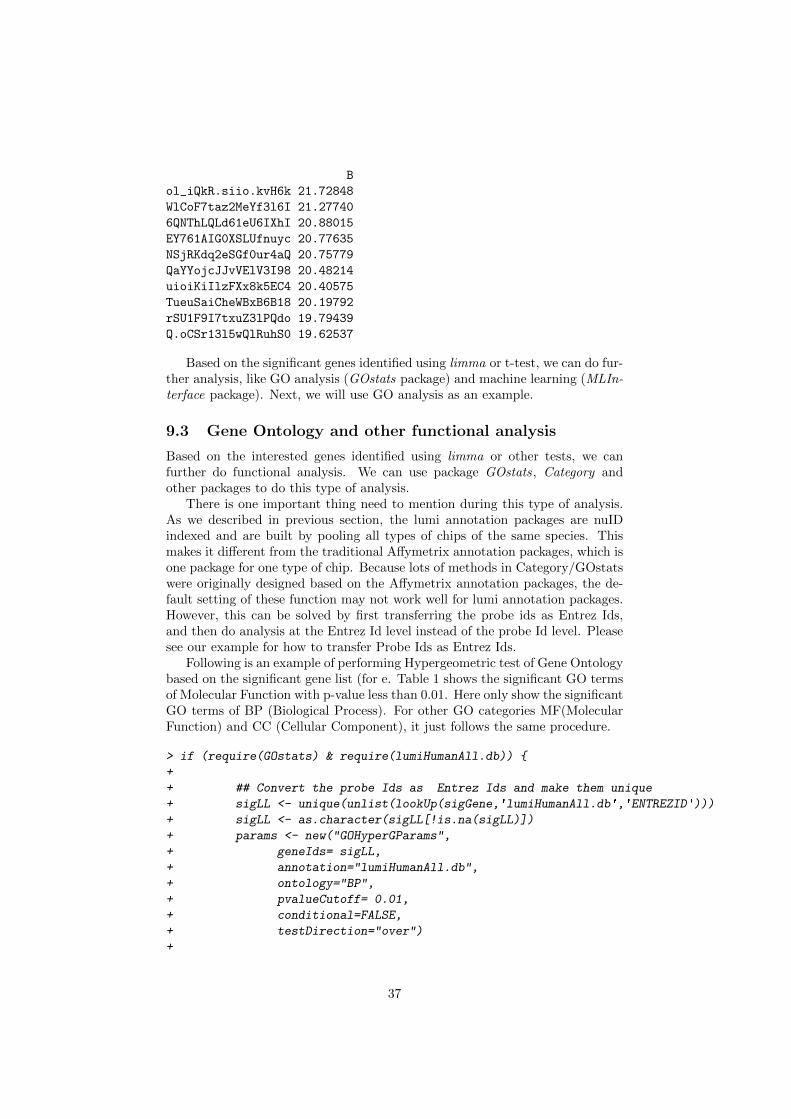
Based on the significant genes identified using limma or t-test, we can do fur-ther analysis, like GO analysis (GOstats package) and machine learning (MLIn-terface package). Next, we will use GO analysis as an example.

9.3 Gene Ontology and other functional analysis

Based on the interested genes identified using limma or other tests, we canfurther do functional analysis. We can use package GOstats, Category andother packages to do this type of analysis.

There is one important thing need to mention during this type of analysis.As we described in previous section, the lumi annotation packages are nuIDindexed and are built by pooling all types of chips of the same species. Thismakes it different from the traditional Affymetrix annotation packages, which isone package for one type of chip. Because lots of methods in Category/GOstatswere originally designed based on the Affymetrix annotation packages, the de-fault setting of these function may not work well for lumi annotation packages.However, this can be solved by first transferring the probe ids as Entrez Ids,and then do analysis at the Entrez Id level instead of the probe Id level. Pleasesee our example for how to transfer Probe Ids as Entrez Ids.

Following is an example of performing Hypergeometric test of Gene Ontologybased on the significant gene list (for e. Table 1 shows the significant GO termsof Molecular Function with p-value less than 0.01. Here only show the significantGO terms of BP (Biological Process). For other GO categories MF(MolecularFunction) and CC (Cellular Component), it just follows the same procedure.

> if (require(GOstats) & require(lumiHumanAll.db)) {

+

+ ## Convert the probe Ids as Entrez Ids and make them unique

+ sigLL <- unique(unlist(lookUp(sigGene,'lumiHumanAll.db','ENTREZID')))

+ sigLL <- as.character(sigLL[!is.na(sigLL)])

+ params <- new("GOHyperGParams",

+ geneIds= sigLL,

+ annotation="lumiHumanAll.db",

+ ontology="BP",

+ pvalueCutoff= 0.01,

+ conditional=FALSE,

+ testDirection="over")

+

37

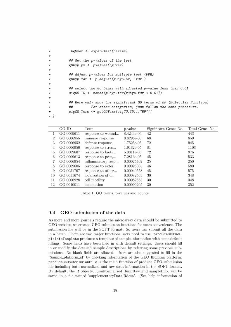
+ hgOver <- hyperGTest(params)

+

+ ## Get the p-values of the test

+ gGhyp.pv <- pvalues(hgOver)

+

+ ## Adjust p-values for multiple test (FDR)

+ gGhyp.fdr <- p.adjust(gGhyp.pv, 'fdr')

+

+ ## select the Go terms with adjusted p-value less than 0.01

+ sigGO.ID <- names(gGhyp.fdr[gGhyp.fdr < 0.01])

+

+ ## Here only show the significant GO terms of BP (Molecular Function)

+ ## For other categories, just follow the same procedure.

+ sigGO.Term <- getGOTerm(sigGO.ID)[["BP"]]

+ }

GO ID Term p-value Significant Genes No. Total Genes No.1 GO:0009611 response to wound... 8.4244e-06 42 4432 GO:0006955 immune response 8.8296e-06 68 8593 GO:0006952 defense response 1.7525e-05 72 9454 GO:0006950 response to stres... 1.9132e-05 81 11035 GO:0009607 response to bioti... 5.0811e-05 72 9766 GO:0009613 response to pest,... 7.2813e-05 45 5337 GO:0006954 inflammatory resp... 0.00025402 25 2508 GO:0009605 response to exter... 0.00026005 46 5809 GO:0051707 response to other... 0.00040553 45 575

10 GO:0051674 localization of c... 0.00082563 30 34811 GO:0006928 cell motility 0.00082563 30 34812 GO:0040011 locomotion 0.00099205 30 352

Table 1: GO terms, p-values and counts.

9.4 GEO submission of the data

As more and more journals require the microarray data should be submitted toGEO website, we created GEO submission functions for users convenience. Thesubmission file will be in the SOFT format. So users can submit all the datain a batch. There are two major functions users need to use. produceGEOSam-

pleInfoTemplate produces a template of sample information with some defaultfillings. Some fields have been filed in with default settings. Users should fillin or modify the detailed sample descriptions by referring some previous sub-missions. No blank fields are allowed. Users are also suggested to fill in the”Sample platform id” by checking information of the GEO Illumina platform.produceGEOSubmissionFile is the main function of produce GEO submissionfile including both normalized and raw data information in the SOFT format.By default, the R objects, lumiNormalized, lumiRaw and sampleInfo, will besaved in a file named ’supplementaryData.Rdata’. (See help information of

38

produceGEOSubmissionFile) Users can include this R data file as a GEO sup-plementary data file.

## Produce the sample information template

> produceGEOSampleInfoTemplate(lumi.example, lib.mapping = 'lumiHumanIDMapping', fileName = "GEOsampleInfo.txt")

## After editing the 'GEOsampleInfo.txt' by filling in sample information

> produceGEOSubmissionFile(lumi.N.Q, lumi.example, lib='lumiHumanIDMapping', sampleInfo='GEOsampleInfo.txt')

10 Session Info

> toLatex(sessionInfo())

� R version 3.2.1 (2015-06-18), x86_64-unknown-linux-gnu

� Locale: LC_CTYPE=en_US.UTF-8, LC_NUMERIC=C, LC_TIME=en_US.UTF-8,LC_COLLATE=C, LC_MONETARY=en_US.UTF-8, LC_MESSAGES=en_US.UTF-8,LC_PAPER=en_US.UTF-8, LC_NAME=C, LC_ADDRESS=C, LC_TELEPHONE=C,LC_MEASUREMENT=en_US.UTF-8, LC_IDENTIFICATION=C

� Base packages: base, datasets, grDevices, graphics, methods, parallel,stats, stats4, utils

� Other packages: AnnotationDbi 1.30.1, Biobase 2.28.0,BiocGenerics 0.14.0, DBI 0.3.1, GenomeInfoDb 1.4.1, IRanges 2.2.5,RSQLite 1.0.0, S4Vectors 0.6.1, XML 3.98-1.3, annotate 1.46.0,limma 3.24.12, lumi 2.20.2, lumiHumanAll.db 1.22.0,lumiHumanIDMapping 1.10.0, org.Hs.eg.db 3.1.2

� Loaded via a namespace (and not attached): BiocInstaller 1.18.3,BiocParallel 1.2.7, Biostrings 2.36.1, GEOquery 2.34.0,GenomicAlignments 1.4.1, GenomicFeatures 1.20.1,GenomicRanges 1.20.5, KernSmooth 2.23-15, MASS 7.3-42, Matrix 1.2-1,RColorBrewer 1.1-2, RCurl 1.95-4.7, Rcpp 0.11.6, Rsamtools 1.20.4,XVector 0.8.0, affy 1.46.1, affyio 1.36.0, base64 1.1, beanplot 1.2,biomaRt 2.24.0, bitops 1.0-6, bumphunter 1.8.0, codetools 0.2-11,colorspace 1.2-6, digest 0.6.8, doRNG 1.6, foreach 1.4.2,futile.logger 1.4.1, futile.options 1.0.0, genefilter 1.50.0, grid 3.2.1,illuminaio 0.10.0, iterators 1.0.7, lambda.r 1.1.7, lattice 0.20-31,locfit 1.5-9.1, magrittr 1.5, matrixStats 0.14.2, mclust 5.0.1,methylumi 2.14.0, mgcv 1.8-6, minfi 1.14.0, multtest 2.24.0, nleqslv 2.8,nlme 3.1-121, nor1mix 1.2-0, pkgmaker 0.22, plyr 1.8.3,preprocessCore 1.30.0, quadprog 1.5-5, registry 0.2, reshape 0.8.5,rngtools 1.2.4, rtracklayer 1.28.6, siggenes 1.42.0, splines 3.2.1,stringi 0.5-5, stringr 1.0.0, survival 2.38-3, tools 3.2.1, xtable 1.7-4,zlibbioc 1.14.0

11 Acknowledgments

We would like to thanks the users and researchers around the world contributeto the lumi package, provide great comments and suggestions and report bugs.

39

Especially, we would like to thanks Michal Blazejczyk, Peter Bram, Ligia Bras,Vincent Carey, Kevin Coombes, Sean Davis, Jean-Eudes DAZARD, Ryan Gor-don, Wolfgang Huber, DeokHoon Kim, Matthias Kohl, Danilo Licastro, EzhouLori Long, Renee McElhaney, Martin Morgan, Ingrid H. G. stense, DeniseScholtens, Wei Shi, Gordon Smyth, Michael Stevens, Jiexin Zhang (sorted bylast name) and many other people not mentioned here.

12 References

1. Du, P., Kibbe, W.A. and Lin, S.M., (2008) ’lumi: a pipeline for processingIllumina microarray’, Bioinformatics 24(13):1547-1548

2. Lin, S.M., Du, P., Kibbe, W.A., (2008) ’Model-based Variance-stabilizingTransformation for Illumina Microarray Data’, Nucleic Acids Res. 36, e11

3. Du, P., Kibbe, W.A. and Lin, S.M., (2007) ’nuID: A universal namingschema of oligonucleotides for Illumina, Affymetrix, and other microarrays’,Biology Direct, 2, 16.

4. Barnes, M., Freudenberg, J., Thompson, S., Aronow, B. and Pav-lidis,P. (2005) ”Experimental comparison and cross-validation of the Affymetrix andIllumina gene expression analysis platforms”, Nucleic Acids Res, 33, 5914-5923.

40

Documents

Using lumi, a package processing Illumina Microarray · Using lumi, a package processing Illumina Microarray Pan Duz, Gang Fengzy, Warren A. Kibbezz, Simon Linzx July 4, 2015 zRobert