Using Labor Supply Elasticities to Learn about Income

Policy Research Working Paper 9102

Using Labor Supply Elasticities to Learn about Income Inequality

The Role of Productivities versus Preferences

Katy Bergstrom William Dodds

Development Economics Development Research GroupJanuary 2020

Produced by the Research Support Team

Abstract

The Policy Research Working Paper Series disseminates the findings of work in progress to encourage the exchange of ideas about development issues. An objective of the series is to get the findings out quickly, even if the presentations are less than fully polished. The papers carry the names of the authors and should be cited accordingly. The findings, interpretations, and conclusions expressed in this paper are entirely those of the authors. They do not necessarily represent the views of the International Bank for Reconstruction and Development/World Bank and its affiliated organizations, or those of the Executive Directors of the World Bank or the governments they represent.

Policy Research Working Paper 9102

This paper argues that labor supply elasticities encode infor-mation about the determinants of income inequality. In the theoretical framework, individuals choose labor supply conditional on productivities and preferences for consump-tion relative to leisure. The paper shows that reduced-form labor supply elasticities allow one to isolate the components of income due to productivities versus preferences. The

paper then investigates what labor supply elasticities imply about the importance of productivities versus preferences in the United States. Estimates from the literature imply pro-ductivities drive most of income inequality. Larger income effects and larger differences between income and hours worked elasticities imply preferences play an increasingly important role.

This paper is a product of the Development Research Group, Development Economics. It is part of a larger effort by the World Bank to provide open access to its research and make a contribution to development policy discussions around the world. Policy Research Working Papers are also posted on the Web at http://www.worldbank.org/prwp. The authors may be contacted at [email protected].

Using Labor Supply Elasticities To Learn About

Income Inequality: The Role of Productivities versus

Preferences ∗

Katy Bergstrom† William Dodds‡

Keywords: income inequality, productivity, preference, labor supply elasticityJEL Codes: D63, J22, H21, H31

∗We would like to thank our advisors, Doug Bernheim, Raj Chetty, and Caroline Hoxby for theirguidance and support on this project. We would also like to thank Jose Maria Barrero, PascalineDupas, Petra Persson, Alessandra Peter, Luigi Pistaferri, Juan Rios, Florian Scheuer, and Isaac Sorkinfor helpful advice, as well as participants at various seminars at Stanford University for their usefulcomments. Finally, thanks to The Ric Weiland Graduate Fellowship in the School of Humanities andSciences, the B.F. Haley and E.S. Shaw Fellowship for Economics, and the Arthur and Eva KaraszFellowship for financial support.†Development Research Group, World Bank. Email: [email protected].‡Charles River Associates. Email: [email protected].

1 Introduction

The determinants of income inequality are a contentious topic of debate among economists,

politicians, and policy makers alike. Many factors, such as family background, demo-

graphics, discrimination, genetics, luck, and work ethic play a role in determining eco-

nomic success. All of these factors ultimately contribute to two higher level determinants

of labor income inequality: (1) differences in productivities, i.e., ability to transform labor

into personal income, and (2) differences in preferences, i.e., desire for consumption rel-

ative to leisure.1 Note our definition of preferences is narrow in that it refers only to the

taste for consumption relative to leisure whereas our definition of productivity is broad

in that it encompasses not only things like intelligence or social skills but also things like

human capital acquisition, discrimination, or rent seeking, which all ultimately impact

ones ability to transform labor into income.

Understanding the determinants of income inequality is important because social wel-

fare gains associated with redistribution depend on why we have inequality. A number

of studies have shown that individuals’ redistributive tastes may be influenced by how

much of income inequality is driven by preferences. In experimental settings, individuals

appear less inclined toward redistribution when income differences are due to differences

in preferences, which manifests as differential effort (e.g., Hoffman et al. (1994), Cherry

et al. (2002), or Rey-Biel et al. (2011)). Moreover, Alesina et al. (2001) find that

countries in which individuals believe income is driven primarily by preference differences

tend to have less redistributive policies. Hence, individuals’ normative tastes for redistri-

bution appear to depend on the sources of income inequality; thus, examining the extent

to which income inequality is driven by productivity vs. preference heterogeneity is a

positive step towards understanding the welfare benefits of redistribution.2

This paper shows that we can use information encoded in labor supply elasticities to

learn about the extent to which labor income inequality is driven by heterogeneity in

productivities vs. heterogeneity in preferences for consumption relative to leisure. To

see why labor supply elasticities contain information about income inequality, consider a

population of individuals in a static world who choose how many hours to work conditional

on heterogeneous productivities and preferences over the consumption/leisure trade-off.

To simplify ideas, assume productivity is equivalent to the hourly wage rate. In this

canonical world, labor income inequality can first be decomposed into differences in hourly

1We will focus solely on labor income inequality throughout this paper.2However, decomposing income inequality into productivities and preferences is not necessarily com-

plete; if individuals have redistributive preferences which depend on the determinants of productivitiesand preferences, then a more complete decomposition of income inequality will be needed to assess thewelfare benefits of redistribution. For example, individuals may have different tastes for redistributionif preference heterogeneity is mostly due to innate disutility of labor vs. disutility of labor due to poorhealth. Nonetheless, even if this is the case, our work is a useful step towards better understanding thesources of income inequality.

1

wages and differences in hours worked (such a decomposition is explored in, for example,

Haider, 2001 or Blundell et al., 2018). Going a step further, heterogeneity in hours

worked is driven not only by differences in preferences over the labor/leisure trade-off,

but also by differences in wages (productivities), which lead to gross substitution effects

as higher wage individuals shift toward labor (or toward leisure if the labor supply curve

is backward bending). The labor supply elasticity of hours worked with respect to the

wage rate tells us how we expect hours worked to change with the wage rate, holding

preferences over the consumption/leisure trade-off constant. Thus, we can use the labor

supply elasticity to net out the component of hours worked due to wage effects, leaving

us with the component of hours worked attributable to preference differences. Finally,

we can use the component of hours worked attributable to preferences to understand how

much of income inequality is due to preference heterogeneity.

We formalize this intuition by developing a method to assess the extent to which cross-

sectional labor income inequality is driven by productivities vs. preferences, using only

empirically observable labor supply elasticities, in the context of a general labor supply

model. To begin, we consider a static neo-classical labor supply model in which produc-

tivity is equivalent to the hourly wage; we later relax this assumption. Preferences are

captured by a single parameter that changes the marginal rate of substitution between

consumption and leisure. Conditional on heterogeneous productivities and preferences,

agents choose hours worked to maximize utility. This agent optimization problem defines

a function between primitives (productivities and preferences) and labor supply decisions

(incomes and hours worked). We show how to invert this function, i.e., how to infer

primitives from observable decision variables; this allows us to investigate the role pro-

ductivities and preferences play in driving income inequality. The principle finding is

that we can express this inverse function entirely in terms of reduced form labor sup-

ply elasticities, thereby yielding a transparent procedure that highlights the manner in

which labor supply elasticities encode information about the drivers of income inequal-

ity. Towards understanding this result, consider comparing preferences for consumption

relative to leisure between a high wage individual who works many hours and a low wage

individual who works fewer hours. The labor supply elasticity tells us how hours worked

should vary between a high wage person and a low wage person, holding preferences

constant. Thus, we can use the labor supply elasticity to subtract out the component of

hours worked due to wage effects and then use the component of hours worked solely due

to preferences to compare preferences between the high wage person and the low wage

person. Essentially, labor supply elasticities encode information about income inequality

as they allow us to infer individual preferences from the component of hours worked that

is not driven by wage differences.

Our baseline model assumes that all individuals are able to optimally adjust their

income on the intensive margin. We show that labor supply elasticities still contain

2

information about income inequality even if individuals face labor market frictions so

that labor supply is not perfectly flexible. Our method can be adapted to determine the

extent to which income inequality is driven by productivities (hourly wages), preferences,

and frictions if we can elicit how much individuals would ideally like to work (for example,

via survey) and the elasticity of ideal hours worked with respect to the wage rate.3

We then show that labor supply elasticities still encode information about income

inequality if we relax the assumption that productivity is equivalent to the hourly wage.

We consider a world in which individuals choose (unobserved) effort per hour in addition

to hours of work. In this setup, hourly wage is equal to effort per hour multiplied by

productivity (thus, productivity is now equal to an unobservable effort wage). Our main

result is that we can still invert the function between productivities and preferences and

incomes and hours worked as long as we observe the labor supply elasticities of both

income and hours worked with respect to the effort wage, or equivalently the tax rate.

We can do this inversion because the function mapping productivities and preferences

to labor supply decisions has a derivative matrix that can be expressed entirely in terms

of observable labor supply elasticities; hence, we can invert this observable matrix to

find the derivative matrix of the inverse function, which in turn allows us to recover the

entire inverse function (up to an irrelevant normalization). Thus, our method allows us

to investigate the extent to which productivities (effort wages) and preferences impact

income inequality using only four estimable labor supply elasticities: the taxable income

and hours worked elasticities, both compensated and uncompensated, with respect to the

tax rate.4

We then show that labor supply elasticities still contain information about income

inequality even if productivity (the rate at which one transforms labor into personal in-

come) is partially determined by prior human capital decisions. We explore a dynamic

labor supply model with human capital acquisition and endogenous wage growth. We

show that we can use labor supply elasticities to invert the relationship between observ-

ables (incomes and hours) and current productivities and preferences, recognizing that

current productivities are determined both by innate skills as well as past labor supply

and human capital decisions (which are choice variables and therefore functions of both

innate skills and preferences). Thus, labor supply elasticities allow us to recover cross-

sectional productivities and preferences using labor supply elasticities. Intuitively, this

yields a lower bound as to the extent that preferences drive income inequality because

some of the variation in productivities may actually be driven by previous human capital

decisions, which are in turn partly driven by preferences.

Next, we illustrate what different labor supply elasticities imply about the drivers of

3While actually identifying the relevant elasticity of ideal hours worked with respect to the wage ratemay be challenging, we discuss in the text two potential, yet imperfect, ways to get at this elasticity.

4The fully general version of our method allows labor supply elasticities to vary across individualsand requires elasticity estimates that vary at the income and hours worked level.

3

income inequality in the U.S. Using several labor supply elasticity estimates and using

data on incomes and hours worked from the American Time Use Survey, we apply our

method to recover individual productivities and preferences.5 We begin with a baseline

set of elasticity parameters taken as averages from a number of labor supply studies

discussed in Chetty (2012). Under the baseline elasticities, we infer high income peo-

ple actually have lower average preferences for consumption compared to middle income

people. Essentially, the baseline labor supply elasticities imply that high income people

should work substantially more than low income individuals; because we observe a rela-

tively flat hours gradient over the income distribution, we infer that high income people

have, on average, lower preferences for consumption relative to leisure. However, we then

vary the elasticity parameters and show that we will infer preferences are increasingly im-

portant in driving income inequality if we use (1) a larger difference between the income

and hours elasticities and/or (2) larger income effects to recover individual productivities

and preferences. Thus, a larger difference between the income and hours elasticities and

larger income effects imply that more of the difference in incomes between rich and poor

is due to preferences.

Finally, to highlight how our findings on the determinants of income inequality change

our understanding of the welfare benefits of redistribution, we simulate optimal tax sched-

ules that account for both productivity and preference heterogeneity driving inequality.

While the general methodology to recover determinants of income inequality devised in

this paper is free of normative assumptions, for the purpose of welfare calculations, we

adopt the normative stance developed in Fleurbaey and Maniquet (2006) in which dif-

ferences in productivities merit redistribution whereas differences in preferences do not

merit redistribution. We simulate optimal tax schedules, accounting for both produc-

tivity and preference heterogeneity, under different values of the relevant labor supply

elasticities and compare these schedules to the optimal tax schedules in which all income

inequality is due to productivity heterogeneity as in Mirrlees (1971) or Saez (2001).

Under our baseline elasticity estimates from Chetty (2012), we find that optimal tax

rates are actually slightly higher than the Mirrleesian reference case in which all income

inequality is due to productivity heterogeneity. Essentially, the elasticity estimates from

Chetty (2012) imply that high income individuals actually have lower preferences for

consumption, on average, than middle income individuals. Therefore, high taxes are even

more desirable than in the Mirrleesian benchmark. However, this finding is sensitive to

the elasticity estimates used to recover individual productivities and preferences. We

find that a larger difference between the income and hours worked elasticities and larger

income effects both imply lower tax rates relative to the Mirrleesian optimal tax schedule.

5Because the literature has not reached a consensus on the magnitudes of the different labor supplyelasticities, and because current data provides imperfect measurements of hours worked, our empiricalapplication aims to investigate how changing labor supply elasticities affects the relative importance ofproductivities vs. preferences in driving income inequality.

4

This is because a larger difference between the income and hours worked elasticities and

larger income effects both imply that high income individuals have higher preferences

for consumption, so that redistributing away from them is less desirable than in the

Mirrleesian benchmark. The takeaway is that labor supply elasticities not only impact

the efficiency costs of taxation, but also encode important information about the equity

benefits of taxation through the information they contain about the drivers of income

inequality.

The rest of the paper proceeds as follows: Section 2 discusses related literature, Section

3 illustrates how labor supply elasticities can be used to recover preferences in the context

of a labor supply model in which productivity is equivalent to the hourly wage and

individuals only choose hours worked, Section 4 extends our analysis when productivity

is not equal to the hourly wage (i.e., individuals choose effort per hour as well as hours

worked), Section 5 discusses our empirical implementation, Section 6 discusses how our

findings impact optimal taxation, and Section 7 concludes.

2 Related Literature

This paper is related to four different strands of literature: (1) decomposing income

inequality empirically into wages and hours, (2) survey evidence on the determinants

of income inequality, (3) the relationship between income inequality determinants and

redistribution, and (4) the invertibility of economic systems.

First, this paper is related to an empirical literature focused on statistically decom-

posing income inequality into wage heterogeneity vs. hours worked heterogeneity. Haider

(2001), for example, decomposes the variance of income into wage and hours worked,

finding that most of income variance is due to wage variance, although a non-negligible

amount of income variance is due to hours variance (and the covariance between hours

and wages). Doiron and Barrett (1996) also find that income variance is driven more by

wage heterogeneity for males; however, they find that the opposite is true for women.

Gottschalk and Danziger (2005) and Blundell et al. (2018) have similar findings. Our

paper contributes to this literature by going a step further and decomposing income in-

equality into productivity and preferences, which is the more relevant decomposition for

welfare analysis; our decomposition recovers preferences from hours worked net of substi-

tution effects and recognizes that productivity may not be equivalent to the hourly wage

if individuals exert differential effort per hour.

Second, while, to the best of our knowledge, this is the first paper that attempts to de-

compose income inequality into productivity heterogeneity vs. preference heterogeneity,

there is a large body of work that investigates individuals’ beliefs over the determinants

of income inequality and how these beliefs relate to views on the merits of redistribu-

tion. Data from the World Values Survey shows Americans are about twice as likely

5

as Europeans to think that the poor are lazy or lack willpower (60% versus 26%) and

that in the long run, hard work usually brings a better life (59% versus 34-43%; Ladd

and Bowman (2001)). Notably, the United States provides far less in welfare assistance

than most European countries. This correlation between beliefs and actual redistribu-

tive policies across countries is reinforced by the findings of Alesina et al. (2001): social

spending (welfare, social security, etc.) as a percentage of GDP is positively correlated

with average beliefs that income inequality is driven by luck as opposed to preferences.

These cross-country findings are further supported by experimental evidence. For

example, Hoffman et al. (1994) use an experiment to show that when agents earn the

right to be the dictator, they give less in the dictator game. Similarly, Cherry et al.

(2002) and Oxoby and Spraggon (2008) show that dictators give (take) less when income

is earned by the dictators (recipients) compared to when income is determined by the

experimenter. Investigating the role of beliefs on the causes of poverty and the differences

in redistribution policy between Spain and the US, Rey-Biel et al. (2011) show that

overall giving between American and Spanish subjects is similar when the actual role

of luck versus effort is known, however, Spanish subjects give more when uninformed

compared to American subjects because American subjects have stronger ex ante beliefs

that effort is the primary driver. In summation, individuals look upon redistribution

towards poorer individuals more favorably when these individuals are perceived to be

poor due to luck as opposed to low preferences for consumption relative to leisure.

Third, there have been a number of papers which explore how determinants of in-

come inequality affect optimal redistribution from a theoretical perspective. For exam-

ple, Boadway et al. (2002), Chone and Laroque (2010), Jacquet and Lehmann (2015),

and Lockwood and Weinzierl (2016) all explore how adding an additional dimension of

heterogeneity in the form of preferences affects different aspects of the tax schedule. For

example, Lockwood and Weinzierl (2016) show that, under certain functional form as-

sumptions, increasing the amount of income inequality due to preferences leads to less

redistributive optimal tax schedules. Our work contributes to this literature by show-

ing, via simulation, how different labor supply elasticity parameters change optimal tax

schedules by impacting the welfare benefits of redistribution (through the implied degree

of preference vs. productivity heterogeneity driving inequality).

Lastly, this paper is related to the literature on invertibility of economic systems. Saez

(2001) shows in a labor supply model with productivity heterogeneity how one can invert

labor supply decisions into productivities using the elastictiy of income with respect to

the tax rate. We extend this result to a model with both preference and productivity

heterogeneity. There is also a vast literature that performs inversions from observables

into unobservables in the context of product demand using structural estimation, either

parametrically (e.g., in Berry et al. (1995)) or non-parametrically (e.g., in Berry and

Haile (2010)). Our method to invert observable labor supply decisions into unobserved

6

primitives uses economic theory to relate the elasticities of observables with respect to

primitives to elasticities of observables with respect to other observables (in our case

tax rates). This allows us to bypass structural estimation of utility functions by using

reduced form elasticity estimates to directly invert the relationship between observables

and primitives. Our method is useful conceptually towards understanding the relationship

between primitives (productivities and preferences) and observable labor supply decisions.

Moreover, our method is perhaps more transparent than a structural approach in revealing

the variation driving the inversion; this is especially important in our labor supply context

as it enables us to identify the particular features of the data that lead to the estimated

income inequality decomposition.

3 Baseline Model

We begin with a simple, static labor supply model with no labor market frictions in

which productivity is equivalent to hourly wage. Individuals have only one dimension of

labor supply: hours worked. We show that we can use labor supply elasticities to invert

the relationship between observables and primitives in this stylized world. Because the

insights of this baseline framework will carry over to more general cases, it is useful to

highlight the underlying mechanisms in this simplified setting.

3.1 Problem Setup

Suppose individuals have preferences over hours worked, h, and consumption, c, and

that they vary in terms of their productivity, n, and preferences for consumption relative

to leisure, α. Productivity affects the return to labor, with income z = nh, whereas

preferences affect the marginal rate of substitution between consumption and leisure.

Denoting the (linear) tax rate as T ′ and the guaranteed income level R, the individual’s

problem can be written as:6 7

maxh

αu(c)− v(h)

s.t. c ≤ nh(1− T ′) +R

The associated first order condition is given by:

αn (1− T ′)u′ (nh∗(1− T ′) +R)− v′(h∗) = 0 (1)

6We assume a linear tax rate first for expositional simplicity, but we consider piece-wise linear taxschedules with increasing marginal tax rates in Appendix A.4 in the context of the model in Section 4,which nests our baseline model.

7The assumption of additive separability is not necessary. Appendix A.5 shows how the analysiscarries over to the non-separable case in the context of our more general baseline model with effortdecisions.

7

(a) Heterogeneity in Productivities n (b) Heterogeneity in Preferences α

Figure 1: Heterogeneity in Productivities vs. Heterogeneity in Preferences

In the above setup, n determines one’s budget set and α determines the consump-

tion/leisure bundle chosen conditional on a given budget set. Graphically, heterogeneity

in n leads to differences in slopes of budget constraints (Panel 1a), whereas heterogene-

ity in α leads to heterogeneity in slopes of indifference curves (Panel 1b) as in Figure

1. We assume that preference heterogeneity enters the utility function by scaling the

marginal rate of substitution between consumption and leisure; we believe that this form

of preference heterogeneity is both sensible and reasonably general.8

The goal of this paper is to show how we can use labor supply elasticities to determine

the extent to which income inequality is driven by heterogeneity in productivities n vs.

preferences α. More concretely, we will use labor supply elasticities to determine (1) every

person’s (n, α) and (2) the function that maps primitives (n, α) to optimal incomes z∗.

However, there are many (n, α) combinations that will choose the same level of income;

hence, we cannot directly infer individuals (n, α) from their income alone. Suppose

additionally that we observe individuals’ optimal hours worked, h∗.9 In this case, there

is some function G which maps primitives, expressed in terms of logs for convenience,

(log(n), log(α)) ∈ N × A to (observable) optimal levels of income and hours worked,

(log(z∗), log(h∗)) ∈ Z∗ × H∗, G : N × A → Z∗ × H∗.10 We show that this function G

has an inverse; we will show that we can express the inverse of this function G−1, which

8Ultimately, our method will recover a preference parameter α for each individual. Even if we mis-specify the way in which preferences enter the utility function, we show in Appendix A.6 that our methodstill recovers the correct ordinal preference parameter rankings for all individuals as long as income (orequivalently hours worked) is increasing in the preference parameter (however it truly enters the utilityfunction).

9We assume throughout that we can, at least in principle, observe individuals’ choices of optimalincomes and hours without error.

10Such a function will exist as long as each (n, α) has a unique optimum (z∗, h∗); this holds given aconstant tax rate under standard concavity assumptions on the utility function (u′′(c) ≤ 0 and −v′′(h) ≤0).

8

maps observables to primitives, entirely in terms of reduced form labor supply elasticities.

Once we know G−1, we can find G, which allows us to analyze the extent to which income

inequality is due to differences in n vs. differences in α.

It is worth mentioning that an alternative route to determining n and α in the above

model would be to make functional form assumptions on u(·) and v(·) (or parametrize

these from data in some fashion) and use the individual first order condition to determine

the value of n and α that would choose to optimally work hours h∗ and earn income z∗.

The key theoretical insight of this section is that we can instead use observable labor

supply elasticities to recover G−1 without making any functional form assumptions on

u(·) or v(·). By expressing G−1 in terms of a few observable elasticities, our sufficient

statistics approach explicitly identifies how key economic parameters affect our inferences

around the sources of income inequality. Before deriving G−1, we now take a short detour

to define the relevant elasticity concepts.

3.2 Defining Labor Supply Elasticities

The primary elasticities of interest in this paper are elasticities of choice variables, such

as hours worked, with respect to productivities n or preferences α. While this section

will focus on elasticities of hours worked, we define elasticities more generally as we will

discuss elasticities of other choice variables (e.g., effort or income) later in subsequent

sections. We define elasticities of choice variable i w.r.t. n and α, respectively, as:

ξni ≡∂ log(i∗)

∂ log(n)

ξαi ≡∂ log(i∗)

∂ log(α)

We also define the uncompensated elasticity of a choice variable i w.r.t. the tax rate as:

ξui ≡∂ log(i∗)

∂ log(1− T ′)

We similarly define the income effect parameter as:

ηi ≡ z∗(1− T ′)∂ log(i∗)

∂R

Finally, we define ξci ≡∂ log(i∗)

∂ log(1−T ′)

∣∣c

as the compensated elasticity. By the Slutsky Equa-

tion, we have the following relationship:11

11 If the choice variable i is hours worked, the Slutsky equation states: ∂ log(h∗)∂ log(1−T ′) = ∂ log(h∗)

∂ log(1−T ′)∣∣c

+

n(1 − T ′)∂h∗

∂R . This is the standard labor supply Slutsky equation (recognizing that n(1 − T ′) is the

after-tax wage, ∂ log(h∗)∂ log(1−T ′) = ∂ log(h∗)

∂ log(n(1−T ′)) and ∂ log(h∗)∂ log(1−T ′)

∣∣c

= ∂ log(h∗)∂ log(n(1−T ′))

∣∣c). If the choice variable i is

income z, this Slutsky equation is the same as in Saez (2001).

9

ξui = ξci + ηi

Before we move on, note that in our labor supply model in which individuals only choose

hours worked, the tax elasticities of incomes and hours worked are identical because

agents have only one margin of adjustment: ξuz = ξuh and ξcz = ξch.

3.3 Recovering Productivities and Preferences Using Labor Sup-

ply Elasticities

We now proceed to derive the function G−1 : Z∗×H∗ → N ×A in terms of labor supply

elasticities. First, we can immediately recover each individual’s productivity n as it is

simply equal to the hourly wage; so if we observe incomes, z∗, and hours worked, h∗, we

can recover n = z∗/h∗. But how can we recover each person’s value of α from z∗, h∗, and

labor supply elasticities? The first step towards recovering preferences α is understanding

the relationship between hours worked and primitives. Hence, we state the following two

Lemmas:

Lemma 3.1. The elasticity of hours worked w.r.t. n, ξnh , is equal to the uncompensated

tax elasticity of hours worked, ξuh .

Proof. See Appendix A.1.

The intuition for Lemma 3.1 is that changing n changes the relative price of leisure

and generates an income effect. Similarly, changing the tax rate also leads to a change

in the relative price of leisure as well as an income effect.

Lemma 3.2. The elasticity of hours worked w.r.t. α, ξαh , is equal to the compensated tax

elasticity of hours worked, ξch.


The intuition behind Lemma 3.2 is that changing α leads to a change in the price of

leisure. Similarly, changing the tax rate also leads to a change in the price of leisure;

however, changing the tax rate also leads to an income effect. Heuristically, changing α

leads to the same effect on hours worked as a change in the tax rate if we subtract out the

income effect caused by the change in tax rates. But by the Slutsky equation, changing

the price of leisure and subtracting out the income effect is the compensated elasticity;

hence the elasticity of hours w.r.t. α is the same as the compensated tax elasticity.

Lemmas 3.1 and 3.2 yield the following two partial differential equations, respectively:

∂ log(h∗(n, α))

∂ log(n)=∂ log(h∗(n, α))

∂ log(1− T ′)= ξuh(n, α) (2)

10

∂ log(h∗(n, α))

∂ log(α)=∂ log(h∗(n, α))

∂ log(1− T ′)

∣∣∣∣c

= ξch(n, α) (3)

Note, h∗(n, α) and z∗(n, α) refer to the optimal incomes and hours chosen by individual

(n, α). To isolate the key economic ideas underlying the inversion between incomes and

hours worked and primitives, let us assume that the tax elasticities ξuh and ξch are constant.

We will relax this assumption in the more general setup of Section 4. Under this constant

elasticity assumption, we can trivially solve the system of partial differential equations

given by 2 and 3, where k is a constant:

log(h∗) = k + ξuh log(n) + ξch log(α) (4)

Using the fact that log(n) = log(z∗) − log(h∗), we can solve for log(α) from Equation 4

by normalizing k = 0 (which is without loss of generality as it just rescales preference

parameters):

log(α) =log(h∗)− ξuh log(n)

ξch=

log(h∗)− ξuh(log(z∗)− log(h∗))

ξch(5)

But Equation 5 expresses α in terms of z∗, h∗ and labor supply elasticities. Hence, we

have recovered the inverse function that maps incomes and hours back to primitives in

our simple labor supply model with constant elasticities:

Proposition 3.3. We can recover G−1 : Z∗ ×H∗ → N × A from the elasticities ξch and

ξuh as long as ξch > 0:

(log(n), log(α)) = G−1(log(z∗), log(h∗)) =

(log(z∗)− log(h∗),

log(h∗)− ξuh(log(z∗)− log(h∗))

ξch

)The key economic intuition behind Proposition 3.3 comes from the equation log(α) =

log(h∗)−ξuh log(n)

ξch. The idea is that hours worked reveals information on preferences for con-

sumption relative to leisure, but it is contaminated by substitution effects from different

wage levels. In other words, we cannot directly infer preferences by examining hours

worked because hours worked is a choice variable that depends on preferences as well as

the hourly wage. In order to recover preferences for consumption relative to leisure we

need to net out the component of labor supply due to wage effects; i.e., we need to deter-

mine hours worked conditional on having the same wage. As such, we subtract out the

effect of wages on hours worked, ξuh log(n), to determine the component of hours solely due

to preferences, i.e., hours worked conditional on a common wage level: log(h∗)−ξuh log(n).

Because hours worked is increasing with preferences, we can then compare this mea-

sure of hours conditional on a common wage, log(h∗) − ξuh log(n), to rank individuals’

preferences for consumption relative to leisure. However, we can go a step further and

11

recover each individual’s α by recalling that hours worked, conditional on a wage level,

increases with log(α) at rate ξch by Lemma 3.2. We divide our measure of hours worked

conditional on a common wage level by ξch to find the log(α) associated with each hours

worked conditional on a common wage level.12

At this point, we believe it is useful to discuss an example. Consider comparing α

between two individuals: an engineer making $30/hour working 60 hours/week and a

mechanic making $10/hour working 40 hours/week. In order to compare preferences

α between the engineer and the mechanic we cannot simply compare the engineer’s

60 hours/week with the mechanic’s 40 hours/week because their different wage lev-

els induce them to work different amounts. Hence, we subtract out the wage effects

on hours worked and find the hypothetical hours worked for the engineer, conditional

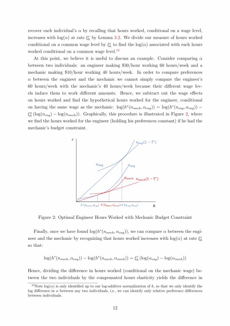
on having the same wage as the mechanic: log(h∗(nmech, αeng)) = log(h∗(neng, αeng)) −ξuh (log(neng)− log(nmech)). Graphically, this procedure is illustrated in Figure 2, where

we find the hours worked for the engineer (holding his preferences constant) if he had the

mechanic’s budget constraint.

Figure 2: Optimal Engineer Hours Worked with Mechanic Budget Constraint

Finally, once we have found log(h∗(nmech, αeng)), we can compare α between the engi-

neer and the mechanic by recognizing that hours worked increases with log(α) at rate ξchso that:

log(h∗(nmech, αeng))− log(h∗(nmech, αmech)) = ξch (log(αeng)− log(αmech))

Hence, dividing the difference in hours worked (conditional on the mechanic wage) be-

tween the two individuals by the compensated hours elasticity yields the difference in

12Note log(α) is only identified up to our log-additive normalization of k, so that we only identify thelog difference in α between any two individuals, i.e., we can identify only relative preference differencesbetween individuals.

12

preferences between the engineer and the mechanic.

To recap, we have shown that we can recover individual preference parameters by in-

verting the function between primitives and labor supply decisions using just two observ-

able labor supply elasticities. The key economic insight is that labor supply elasticities

allow us to compare preferences for consumption relative to leisure across individuals

with different hourly wages by subtracting out the component of hours worked due to

wage effects. The component of hours worked not due to wage effects (i.e., the compo-

nent of hours worked attributable to preferences) then allows us to compare individual

preferences.

3.4 Labor Supply Frictions

Our results so far have relied on the assumption that individuals can perfectly opti-

mize their labor supply by changing hours worked on the intensive margin. There is

a non-negligible subset of people for whom this is probably a reasonable assumption

(e.g., Uber drivers or the self-employed or commission workers); we can immediately

apply our method to use labor supply elasticities to learn about the drivers of income

inequality within this subset of the population. On the other hand, many individuals do

face labor demand inelasticity or market frictions; we provide an imperfect, yet easily

implementable, modification to recover productivities and preferences using labor supply

elasticities if individuals face frictions. Labor market frictions lead to two issues in apply-

ing our method: (1) individuals’ observed hours are no longer equivalent to their optimal

hours and (2) elasticities of observed hours with respect to the tax rate, which reflect

both labor market frictions as well as how optimal choices change with tax rates, are no

longer equivalent to elasticities of optimal hours with respect to primitives (as in Lemmas

3.1 and 3.2). Towards broadening the applicability of our method, consider a world in

which all individuals (n, α) choose an optimal hours worked h∗(n, α) yet face labor supply

frictions. Thus, each individual (n, α) ends up working h(n, α) = h∗(n, α) + εn,α, where

εn,α is some deviation from optimal hours (it does not matter what causes this deviation

from optimal hours).

Even with frictions that prevent individuals from working their optimal number of

hours, we can still learn about the role of productivities vs. preferences in driving income

inequality from labor supply elasticities. To solve the first issue that observed hours are

not equal to optimal hours, suppose that we were able to elicit (via survey, for example)

individuals’ true optimal hours worked h∗.13 Productivity is equal to observed income

divided by observed hours, n = z/h, and optimal income is given by optimal hours h∗

multiplied by n: z∗ = nh∗ = (z/h)h∗.

13For example, the National Study of the Changing Workforce asks people how many hours they wouldprefer to work.

13

There are at least two ways to deal with the second issue that observed hours elasticities

are not equivalent to optimal hours elasticities. First, we could estimate, via survey, the

elasticity of optimal hours worked to the tax rate (by asking individuals their preferred

hours worked under their current wage before and after a tax change). This would

allow us to directly recover G−1 as in Proposition 3.3 using optimal hours h∗, optimal

income z∗, and the elasticities of preferred hours. Alternatively, suppose that some known

set of individuals have εn,α = 0, so that their observed hours worked is equal to their

optimal hours worked as they face no frictions (e.g., Uber drivers or the self-employed

or commission workers). If we can estimate labor supply elasticities for this subset of

individuals with εn,α = 0, then we could recover G−1 exactly as in Proposition 3.3 using

optimal hours h∗, optimal income z∗, ξnh = ξuh |εn,α=0 and ξαh = ξch|εn,α=0. Such a procedure

will allow us to determine the extent to which income inequality is driven by productivity

heterogeneity, preference heterogeneity, and frictions. While this subsection contains no

additional theoretical insights beyond Proposition 3.3, we believe it may be useful for

empirical applications of the method.

Next, we show that we can still use labor supply elasticities to learn about the drivers

of income inequality even if we relax the assumption that productivity is equal to hourly

wage.

4 What if Productivity Differs from Hourly Wage?

While the baseline model in Section 3 is useful to conceptualize how preferences can be

inferred from hours worked by subtracting out wage effects on hours worked, it abstracts

from the possibility that productivity is not equivalent to the hourly wage. Why might

productivity, the rate at which people transform labor into income, differ from the hourly

wage? Previous studies, both theoretical and empirical, have stressed the importance of

accounting for effort per hour decisions in labor supply models, e.g., Atkinson and Stiglitz

(1976), Pencavel (1977), Lin (2003), and Green (2001). If individuals differ in terms of

the effort they exert per hour, hourly wage is equal to effort per hour multiplied by

productivity (which is then an effort wage). Returning to our previous example of the

engineer and mechanic, it may be that in addition to working more hours per week

than the mechanic, the engineer also exerts more effort per hour worked, and therefore

the hours worked variation masks substantially more total labor supply variation (effort

per hour multiplied by hours worked) between the two individuals. We now proceed to

investigate what we can learn about income inequality from labor supply elasticities if

individuals differ in terms of their effort per hour.

14

4.1 Recovering Productivities and Preferences with Effort De-

cisions

We consider the following generalized set-up, in which individuals choose both effort per

hour, e, and hours worked, h:14 15

maxh,e

αu(c)− v(h, e)

s.t. c ≤ nhe(1− T ′) +R

In this setup, which nests the model from Section 3, total labor supply is given by

he and is unobservable.16 Unobservability of total labor supply complicates the analysis

because productivity levels n are no longer directly observable. Now we have z = nhe,

so that hourly wages are equal to ne, but because e is not observable we cannot infer

n simply by observing hourly wage.17 More generally, one can interpret this setup as

allowing for two dimensions of labor supply, only one of which, h, is observable to the

economist. However, our model is easily extended to include even more components of

labor supply so that income z = n(h1e1 + h2e2 + ... + hmem). In this case, all we need

to apply our method is to observe optimal income z∗ and one component of labor supply

h∗i (see Appendix A.7).

Our goal is unchanged: show how we can use labor supply elasticities to recover the

function which maps optimal incomes and hours worked to productivities and preferences,

G−1 : Z∗ × H∗ → N × A. Even though we cannot directly observe individual effort e∗,

we show that we are still be able to express (log(n), log(α)) = G−1(log(z∗), log(h∗)) in

terms of labor supply elasticities without any functional form assumptions. As in Section

3, the first step is understanding how differences in n and α manifest into differences in

observables z∗ and h∗:

14As before, we assume that the tax rate is constant. We show how the method can be applied witha piece-wise linear tax schedule with increasing marginal tax rates in Appendix A.4.

15Note, in our baseline model as well as this more general model, we assume that all individuals havethe same level of unearned income. The methodology is also easily adapted to account for differences inunearned income if we can observe unearned income as well as the labor supply elasticities with respectto unearned income. This will allow us to subtract out the effect of unearned income on labor supply,which is entirely analogous to netting out gross substitution effects of different wage levels (see AppendixA.8).

16If the cost of deviating from e = 1 is infinite, then this model is equivalent to the model from Section3.

17This sort of model is discussed in, for example, Atkinson and Stiglitz (1976).

15

Lemma 4.1. The derivative matrix of (log(z∗), log(h∗)) = G(log(n), log(α)) is:

JG(log(n), log(α)) =

[∂ log(z∗)∂ log(n)

∂ log(z∗)∂ log(α)

∂ log(h∗)∂ log(n)

∂ log(h∗)∂ log(α)

](log(n), log(α)) =

[1 + ξuz ξcz

ξuh ξch

](log(n), log(α))


We will no longer assume elasticities to be constant - they now vary with (log(n), log(α)).

The proof of Lemma 4.1 is just an application of the implicit function theorem and the

intuition for Lemma 4.1 is very similar to the intuition for Lemmas 3.1 and 3.2 in the

baseline framework without effort decisions. Changing n leads to an income effect and a

price effect, so leads to the same behavioral effect on hours worked as an uncompensated

tax change; changing α effectively changes the value of consumption, so leads to the same

behavioral effect on hours worked as a compensated tax change. Additionally, Lemma

4.1 tells us how incomes change with n and α, which is important because, unlike the

baseline setup, ξuz 6= ξuh and ξcz 6= ξch (as now individuals can adjust their labor supply on

both the effort and hours worked margins). Because log(z∗) = log(n) + log(h∗) + log(e∗),

changing n affects z∗ directly through a mechanical effect and indirectly through the

behavioral effect n has on optimal labor supply decisions (h∗ and e∗). The behavioral

effect of changing n on z∗ (i.e., the combined effect on h∗ and e∗) is equal to the uncom-

pensated tax elasticity, hence the effect of n on z∗ is equal the mechanical effect plus the

behavioral effect: ξnz = 1 + ξuz . Changing α just leads to a behavioral response of income,

which is again identical to the response from a compensated tax change, so ξαz = ξcz. This

brings us to our main result: we can use observable labor supply elasticities to recover

the function between incomes and hours and productivities and preferences:

Proposition 4.2. We can recover G−1 : Z∗×H∗ → N×A from the heterogeneous observ-

able elasticities ξuz (z∗, h∗), ξuh(z∗, h∗), ξcz(z∗, h∗) and ξch(z

∗, h∗) as long as all individuals

(n, α) have elasticities satisfying ξcz > 0, ξch > 0, ξch ≥ ξuh , and ξuz − ξcz > −1.18

Proof. We prove Proposition 4.2 under the assumption of a linear tax rate - the piece-wise

linear case is slightly more complicated due to the presence of kink points. See Appendix

A.4 for a derivation with a piece-wise linear tax rate with increasing marginal tax rates.

Let us define G : N × A → Z∗ × H∗ as the continuously differentiable function

that maps each (log(n), log(α)) to a (log(z∗), log(h∗)).19 Our goal is to find the inverse

function, G−1 : Z∗×H∗ → N×A. By Lemma 4.1, we can recover the Jacobian derivative

18Positive compensated elasticities are standard. Uncompensated elasticities being smaller than com-pensated elasticities (i.e., negative income effects) are also standard. Finally, the assumption ξuz−ξcz > −1means income effects are not so extreme that individuals decrease income by more than $1 in responseto a $1 increase in unearned income.

19G will be continuously differentiable as long as the utility function is twice continuously differentiable.

16

matrix of the function G, denoted JG:20







[1 + ξuz ξcz

ξuh ξch

](log(n), log(α))

We want to show that the mapping G is a homeomorphism onto its image, i.e., that

each (n, α) chooses a unique optimal (z∗, h∗). In order to show that G is homeomor-

phic, we need to first show that its Jacobian has an everywhere non-zero determinant,

which is necessary for local invertibility. Dropping the arguments of the elasticities, the

determinant of the Jacobian is:

(1 + ξuz )ξch − ξczξuh= (1 + ξuz − ξcz + ξcz)ξ

ch − ξcz(ξuh + ξch − ξch)

= (1 + ξuz − ξcz)ξch − ξcz(ξuh − ξch) > 0

The first equality is an identity, the second is algebra, and the inequality comes from

the assumptions that ξcz > 0, ξch > 0, ξch ≥ ξuh , and ξuz − ξcz > −1. Therefore, under

the conditions stated in the proposition, JG has a non-zero determinant. Moreover,

(1 + ξuz ) > 0 (as (1 + ξuz − ξcz) > 0 and ξcz > 0) and ξch > 0 so that JG has positive leading

principle minors, hence is everywhere positive definite. A mapping G on a convex domain

with positive definite Jacobian matrix must be homeomorphic onto its image by Gale and

Nikaido (1965) Theorem 6 (we assume the elasticity conditions hold for all (n, α) ∈ R2+

so that the domain is convex).

Thus, the mapping G is globally invertible; moreover, by the inverse function theorem,

the Jacobian of the inverse mapping G−1 is given by:

JG−1(log(z∗), log(h∗)) =

[∂ log(n)∂ log(z∗)

∂ log(n)∂ log(h∗)

∂ log(α)∂ log(z∗)

∂ log(α)∂ log(h∗)

](log(z∗), log(h∗)) =

[1 + ξuz ξcz

ξuh ξch

]−1(log(z∗), log(h∗))

From here, we simply pick a particular (z∗0 , h∗0) and normalize (log(n(z∗0 , h

∗0)), log(α(z∗0 , h

∗0))) =

(0, 0). Finally, if γ represents a path from (log(z∗0), log(h∗0)) to (log(z∗), log(h∗)), we have

by Stokes’ Theorem:21 [log(n(z∗, h∗))

log(α(z∗, h∗))

]=

[0

0

]+

∫γ

JG−1(r)dr (6)

Evaluating the path integral in Equation 6 allows us to match every optimal choice of

income and hours, (z∗, h∗), to a unique level of (n, α), i.e., to recover G−1. As an example,

20In practice, the observed Jacobian must additionally be consistent with some function G, i.e., theJacobian field must be conservative.

21We require that the set of observed (z∗, h∗) values be path connected.

17

the following parametrization of γ allows us to calculate (n, α) for any (z∗, h∗):[log(n(z∗, h∗))

log(α(z∗, h∗))

]=

[0

0

]+

∫ log(z∗)

log(z∗0 )

JG−1(s, log(h∗0))

[1

0

]ds+

∫ log(h∗)

log(h∗0)

JG−1(log(z∗), s)

[0

1

]ds

Essentially, the logic of Proposition 4.2 is as follows. By Lemma 4.1 we know the

derivative matrix of the function G that maps primitives to incomes and hours worked:

JG. We can invert this Jacobian derivative matrix using the inverse function theorem to

get the inverse Jacobian JG−1 (our elasticity restrictions ensure global invertibility). Then

we integrate the inverse Jacobian JG−1 (which is a function of log(z∗) and log(h∗)) along

a path γ between (log(z∗0), log(h∗0)) and (log(z∗1), log(h∗1)) to determine the difference in

primitives (log(n1), log(α1)) and (log(n0), log(α0)) that optimally choose (log(z∗1), log(h∗1))

and (log(z∗0), log(h∗0)), respectively.22 Graphically, this path integral is depicted in Figure

3.

Figure 3: Illustration of Path Integral from Equation 6

But what’s the intuition behind Proposition 4.2? There are two core ideas. The first

core idea is that preferences are still recovered from the component of hours worked that

is not due to productivity effects. In other words, the intuition from Section 3 holds:

subtracting out the component of hours worked due to productivity still gives us a way

to recover preferences for consumption relative to leisure. However, now productivities

are unobservable because effort per hour is unobservable. The second core idea is that we

can infer an individual’s optimal choice of effort per hour (and hence their productivity

22Differences in (log(n), log(α)) are identified but levels are only pinned down by a normalization. Thisnormalization is without loss as relative productivities and preferences will be sufficient to understandwhat is driving income inequality.

18

from the identity z∗ = nh∗e∗) from his/her optimal choice of income and hours worked

as well as the labor supply elasticities of income and hours worked with respect to the

tax rate.

How can we use labor supply elasticities to infer optimal effort per hour from observable

quantities z∗ and h∗? First, note that log(e∗(log(n), log(α))) = log(z∗(log(n), log(α))) −log(h∗(log(n), log(α))) − log(n). Under the conditions in Proposition 4.2, we can invert

the relationship between (z∗, h∗) and (n, α) so as to write n and α in terms of z∗ and h∗.

Hence, we can also write e∗ as a function of z∗ and h∗. We have that:

log(e∗(log(z∗), log(h∗))) = log(z∗)− log(h∗)− log(n(log(z∗), log(h∗))) (7)

For ease of explanation, let us assume that income effects are negligible. In this case we

can show:23

∂ log(e∗)

∂ log(h∗)(log(z∗), log(h∗)) = −1 +

∂ log(n)

∂ log(h∗)(log(z∗), log(h∗)) =

ξcz − ξchξch

(log(z∗), log(h∗)) (8)

The first equality in Equation 8 comes from differentiating Equation 7 and the second

equality uses the equation for ∂ log(n)∂ log(h∗)

from the inverse Jacobian in Proposition 4.2. Next,

note that ξcz − ξch is equal to the elasticity of effort per hour with respect to the tax rate:

ξcz − ξch =∂ log(z∗)

∂ log(1− T ′)

∣∣∣∣c

− ∂ log(h∗)

∂ log(1− T ′)

∣∣∣∣c

=∂ log(e∗)

∂ log(1− T ′)

∣∣∣∣c

= ξce

Hence, Equation 8 is intuitive: individuals’ optimal effort per hour changes in proportion

to their optimal hours worked in accordance with the ratio of the effort elasticity, ξce =

ξcz − ξch, to the hours elasticity, ξch. Next, we use ∂ log(n)∂ log(z∗)

from the inverse Jacobian in

Proposition 4.2 to show that:

∂ log(e∗)

∂ log(z∗)(log(z∗), log(h∗)) = 0 (9)

Solving the system of partial differential equations given by 8 and 9 allows us to infer

optimal effort for any optimal level of income and hours worked. If we again assume all

relevant elasticities are constant, we have (for some constant k, which we can normalize

to 0 without loss of generality):

log(e∗)(log(z∗), log(h∗)) = k +ξcz − ξchξch

log(h∗)

Hence, by observing both the income and the hours elasticity (with respect to the tax

rate), we can infer optimal effort decisions. Once we infer optimal log(e∗) associated

23See Appendix A.9 for a discussion of where this formula comes from and how it changes with incomeeffects.

19

with each optimal level of (log(z∗), log(h∗)), we can recover log(n) = log(z∗)− log(h∗)−log(e∗(log(z∗), log(h∗))). Finally, we can recover α from optimal hours worked by netting

out the substitution effects of different effort wages n as before using:24

log(α) =log(h∗)− ξuh log(n)

ξch

In summation, the intuition behind Proposition 4.2 has three steps. First, optimal

effort per hour is related to optimal hours worked through the equation: log(e∗) =ξcz−ξchξch

log(h∗); intuitively, optimal effort varies with optimal hours worked in the ratio

of the effort elasticity w.r.t. the tax rate to the elasticity of hours worked w.r.t. the tax

rate. Hence, we can infer optimal effort per hour from optimal hours worked. Second,

once we know optimal effort per hour, we can recover productivity using z∗ = nh∗e∗.

Third, once we have recovered productivity, we can subtract out the component of hours

worked due to productivity effects; the remaining component allows us to recover prefer-

ences.

To solidify ideas, recall our example of the engineer making $30/hour working 60

hours/week and the mechanic making $10/hour working 40 hours/week (assume both

work 50 weeks/year). For purposes of illustration, suppose that the hours elasticity is

half as large as the income elasticity so that the hours and effort elasticities are equal:ξceξch

= 1. Hence:

log(e∗eng/e∗mech) =

ξceξch

log(h∗eng/h∗mech) = log(h∗eng/h

∗mech) = log(60/40)

Thus, e∗eng = 32e∗mech, i.e. the engineer exerts 1.5 times as much effort per hour as the

mechanic. Normalizing e∗mech ≡ 1 and using the fact that hourly wage is equal to ne∗,

we can deduce that the mechanic’s productivity is 10 and the engineer’s productivity

is 20; hence, once we account for effort differences, we infer that the engineer is only

twice as productive as the mechanic as opposed to three times as productive if we assume

productivity is equal to hourly wage. We could then find α for both individuals by netting

out substitution effects using log(α) =log(h∗)−ξuh log(n)

ξch.

We have shown in this section that we can still use labor supply elasticities to infer

individuals’ productivities and preferences even if individuals make unobservable effort

decisions in addition to choosing how many hours to work. Importantly, there are four

key elasticities we need to recover the inverse function used to infer productivities and

24While the formulas are slightly different, this intuition still goes through with heterogeneous elastic-ities. We can still solve the system of differential equations 8 and 9 to find optimal effort as a functionof optimal labor supply decisions (z∗, h∗). We can still find log(n) = log(z∗)− log(h∗)− log(e∗). Finally,we can solve differential equations 2 and 3 (replacing the function arguments as (log(z∗), log(h∗)), whichis again without loss due to invertibility) to find log(h∗) as a function of (log(n), log(α)), and then invertthis function to find log(α) as a function of log(h∗) and log(n).

20

preferences: the uncompensated income and hours elasticities with respect to the tax

rate and the compensated income and hours elasticities with respect to the tax rate

(ξuz , ξuh , ξ

cz, ξ

ch); we will investigate what the magnitudes of these parameters imply about

the sources of income inequality in Section 5.

But before we move on to investigate what empirical labor supply elasticity estimates

imply about income inequality in the U.S., we discuss what we can learn from labor

supply elasticities (i.e., how to interpret our findings) if productivity is partly determined

by prior human capital acquisition (which may in turn have been due to differences in

innate skills or preferences).

4.2 Dynamic Re-Interpretation

All of our results have been derived in the context of a static labor supply model that

abstracts from the possibility that individual productivities are partly due to past labor

supply decisions or human capital acquisition. We show that even if individual productiv-

ities are driven by previous decisions, we can still use labor supply elasticities to recover

individual preferences and productivities, recognizing that productivities are determined

both by innate skills as well as past human capital acquisition. This is still an empirically

interesting object as it tells us how much of income inequality is due to cross-sectional

productivities (at a given point in time) vs. preferences. Moreover, this yields a lower

bound for the extent of income inequality due to preferences. This is because some of the

cross sectional variation in productivities is in part due to differences in past decisions,

which were in turn partially due to differences in preferences.25

Consider a model in which individuals differ in terms of innate skills n0 and preferences

α and first make a human capital decision K, at cost κ(K), and then for the rest of their

life choose effort and hours worked each year conditional on this prior human capital

decision. Furthermore, suppose that individuals’ effort wages grow endogenously over

time. Let us denote this growth rate at time t as qt(ht, et) and the cumulative growth

Qt ≡∏t−1

s=1 qs(hs, es). The individual choice problem can be written as:

max{h}Lt=1,{e}Lt=1,K

L∑t=1

βt [αu(ct)− v(ht, et)]− κ(K)

s.t. ct ≤ n0KQthtet(1− T ′) +R

If we define nt = n0KQt as the endogenous effort wage at time t, then an analogue

to Lemma 4.1 still holds as ξntzt = 1 + ξuzt , ξntht

= ξuht , ξαzt = ξczt , and ξαht = ξcht , see

Appendix A.10. Hence, we can use Proposition 4.2 along with annual data on incomes

25Note, we assume preferences are constant over time; i.e., unlike productivities, we assume preferencesare not affected by prior labor supply and human capital decisions.

21

and hours worked (as well as the corresponding elasticities) to determine the function

G−1 : Z∗t × H∗t → Nt × A. Lastly, we can extend this idea to include savings decisions,

see Appendix A.11.

Analyzing this dynamic setup is useful in so far as it clarifies the interpretation of our

method: we use labor supply elasticities to learn about how much of income inequality

is due to cross-sectional productivities (at a given point in time) vs. preferences. Rec-

ognizing that this is the nature of the exercise, we now proceed to investigate what the

empirically estimated labor supply elasticities imply about the drivers of income inequal-

ity in the context of the U.S.

5 Investigating What Labor Supply Elasticities Im-

ply About Income Inequality in the U.S.

In this section, we apply the methodology laid out in Sections 3 and 4 to data. In order to

recover individual productivities and preferences, Proposition 4.2 tells us that we require

labor supply elasticities of incomes and hours worked with respect to the tax rate. But the

empirical literature has not reached a consensus on the magnitudes of these elasticities.

Thus, the goal of this empirical exercise, which should be viewed primarily as a proof

of concept, is to investigate what different labor supply elasticities imply about income

inequality in the U.S.

Recall from Proposition 4.2 that there are four key labor supply elasticities (more

precisely, elasticity functions) that underlie the inversion between labor supply decisions

and primitives; these four elasticities are contained in the Jacobian matrix of partial

derivatives of primitives with respect to labor supply decisions:

JG−1(log(z∗), log(h∗)) =

[∂ log(n)∂ log(z∗)

∂ log(n)∂ log(h∗)

∂ log(α)∂ log(z∗)

∂ log(α)∂ log(h∗)

](log(z∗), log(h∗)) =

[1 + ξuz ξcz

ξuh ξch

]−1(log(z∗), log(h∗))

While Proposition 4.2 allows for the these elasticities to vary across individuals with differ-

ent incomes and/or hours worked, empirical estimation of labor supply elasticities has, for

the most part, focused on recovering average tax elasticities as opposed to heterogeneous

tax elasticities. Hence, for our baseline estimates of elasticities, we will assume these

elasticities are constant and use the average (compensated) income and hours elasticity

estimates from a number of studies discussed in Chetty (2012): ξcz = 0.15 and ξch = 0.15.26

These parameter estimates correspond to an effort elasticity of 0 (as ξcz − ξch = 0) and

therefore can be interpreted in the context of Section 3, in which productivity is equiv-

alent to hourly wage. Furthermore, consistent with most of the empirical literature on

26Chetty (2012) only discusses average compensated elasticities. Also, we assume that these elasticityvalues correspond only to real responses (as opposed to reporting responses).

22

behavioral responses to taxation (e.g., Blundell and MaCurdy, 1999), we assume that

income effects are negligible (so that ξuz = ξcz and ξuh = ξch).27

After briefly discussing what the baseline results imply about the drivers of income

inequality, our main analysis concerns performing the inversion from labor supply deci-

sions to primitives under different assumptions on the relevant elasticities, highlighting

how deviations from the baseline estimates change our inference about the determinants

of income inequality. We show that (1) larger differences between the income and hours

elasticities with respect to the tax rate (i.e., larger effort elasticities) and (2) larger income

effects will both lead us to infer that preference heterogeneity is increasingly important

in driving income differences between rich and poor. We also discuss briefly at the end of

this section how our findings change if allow for heterogeneity in the elasticity schedules

(roughly in line with the findings of Gruber and Saez, 2002) and how we can account for

labor market frictions using survey data on actual and preferred hours.

5.1 Data on Incomes and Hours Worked

We will use data on incomes and hours worked from the American Time Use Survey

(ATUS), which is a survey conducted on a subset of individuals who have participated

in the CPS.28 In addition to income data, the ATUS asks respondents to meticulously

detail all of their activities on a particular (random) “diary day”. We then assume that

this noisy “diary day” measure is representative of this individual’s average daily hours

worked. We also do not have days worked per year, so we impute that all individuals

work 250 days a year unless they report being part time and work > 8 hours on their

diary day, in which case we impute their days worked as 125. Our sample consists of

all individuals reporting a positive income, thereby abstracting from the possibility of

joint familial labor supply decisions. We show that our findings all hold with the smaller

sample of single individuals, shown in Appendix C.3. We drop individuals who say they

are involuntarily under-employed, hopefully mitigating the effect of labor supply frictions

on our inferences. Our final sample from the ATUS then consists of data on (inflation

adjusted) incomes and diary hours for 34,470 unique individuals from the years 2003-2015.

See Appendix B for more detail on our sample construction.

Our measure of hours worked is noisy due to measurement and aggregation errors.

Importantly, this noisy measure of hours worked is fine for our purposes so long as the

noise is unbiased in the sense that the sample joint distribution of incomes and hours

worked is representative of the true population joint distribution. Even if the sample

27We also assume that all individuals face a constant linear tax rate even though our method is easilyadaptable to tax schedules with kinks, see Appendix A.4. This is for simplicity and consistency with themain body of the text and is likely inconsequential given the lack of bunching in the empirical incomedensity.

28We discuss in Appendix B.2 why we do not use the hours worked measure from the CPS.

23

distribution is not the same as the population distribution, we expect this should not

affect the comparisons between the relative importance of productivities vs. preferences

for different assumptions on the elasticity parameters.

5.2 Baseline Estimates

Using our baseline estimates from Chetty (2012), ξcz = ξuz = ξch = ξuh = 0.15, we can

recover the function G−1(log(z∗), log(h∗)) using the inverse Jacobian from Proposition 4.2.

Applying G−1(log(z∗), log(h∗)) to the observed distribution of incomes and hours worked

from the ATUS yields a value of (n, α) for each individual in our sample. However, this

distribution of productivities and preferences (n, α) is not easily interpreted. Towards

understanding the role productivities and preferences play in driving income inequality,

we will construct the counter-factual income for each individual if (1) everyone had the

same productivity or (2) everyone had the same preferences. Comparing these measures

with actual income will help us understand the extent to which inequality is due to

productivities vs. preferences.29

First, for all individuals (n, α) we will calculate zCFn0= n0h

∗(n0, α)e∗(n0, α), the income

they would optimally earn if they had productivity n0 and preferences α. This is feasible

because we have identified each person’s productivity n and we know the manner in which

both hours worked and effort per hour change with n. Second, for all individuals (n, α) we

calculate zCFα0= nh∗(n, α0)e

∗(n, α0), the income they would earn if they had productivity

n and preferences α0; this exercise is possible because we have identified each individual’s

preferences α and we know how both hours and effort per hour change with α.

In Figure 4a we plot average counter-factual incomes at each actual income level

assuming all individuals had the same n (the baseline level of n0 is chosen so that the

mean income level in the counter-factual income distribution matches the mean income

level in the empirical income distribution). In Figure 4b we plot average counter-factual

incomes at each actual income level assuming all individuals had the the same α (again,

the baseline level of α0 is again chosen so that the mean income level in the counter-factual

income distribution matches the mean income level in the empirical income distribution).

29While this counter-factual income exercise is nominally performed under the assumption that αenters the utility function as αu(c) − v(h, e), all of the counter-factual income measures in this sectionare actually invariant to any functional form of preference heterogeneity for which income monotonicallyincreases in preferences. Conceptually, as long as hours are increasing in preferences, our method recoversthe correct preference rankings among all individuals (even if the nature of preference heterogeneity iswrong due to functional form mis-specification); we show in Appendix A.6 that the counter-factualincomes only depend on these ordinal preference rankings.

24

(a) Average Counter-factual Incomes, same n (b) Average Counter-factual Incomes, same α

Figure 4: Counter-Factual Incomes, Baseline Estimates ξcz = ξuz = ξch = ξuh = 0.15

The first takeaway from Figure 4a is that high income individuals would earn substan-

tially less if all individuals had the same productivities - this is indicated by the large

deviation from the 45◦ line. On the other hand, the average counter-factual income plot

in Figure 4b is relatively close to the 45◦ line, so we infer that only a small amount of

income inequality is due to preference heterogeneity.30 Thus, under our baseline elasticity

estimates, productivity differences are much more important for generating income in-

equality than are preference differences. This should not be surprising given that, under

our baseline elasticity estimates, productivity is equal to the hourly wage and a number of

studies have shown that hourly wage variation drives most of income inequality (Haider

(2001), Doiron and Barrett (1996), Gottschalk and Danziger (2005), and Blundell et al.

(2018)).

But there is more we can learn from labor supply elasticities other than that produc-

tivity heterogeneity is driving most of income inequality. For instance, note in Figure

4a that high income individuals would actually earn less than median income individ-

uals if they all had the same productivity. For example, if everyone had homogeneous

productivities, median income individuals (people making ≈ $35, 000) would earn about

$41,000 on average, whereas high income individuals (people making ≈ $100, 000) would

only earn about $37,000 on average. Additionally, note in Figure 4b that high income

individuals would earn slightly more than in actuality if everyone had the same prefer-

ences. Thus, our baseline elasticity estimates imply the high income individuals have

lower preferences, on average, than middle income individuals.

Why do we infer that high income individuals actually have weaker preferences for

consumption relative to leisure compared to middle income individuals? Essentially, this

is because our baseline labor supply elasticities imply that high income individuals should

work substantially more than low income individuals due to substitution effects. How-

30We plot the counter-factual income distributions in Appendix E.

25

Figure 5: Observed Mean Hours Worked and Predicted Mean Hours Worked UnderConstant Preferences vs. Actual Income, ξcz = ξuz = ξch = ξuh = 0.15

ever, empirically, high income individuals do not work many more hours (on average)

than middle income individuals. Hence, conditional on our baseline elasticity estimates,

this leads us to infer that high income people have weaker preferences. This is depicted

graphically in Figure 5 where we plot observed average hours worked over the income

distribution along with how we expect average hours worked to change if all individu-

als had the same preferences (or if average log(α) was identical for all income levels).

The black dashed line, representing how we expect hours to change with homogeneous

preferences, has a positive slope because we expect higher income individuals to work

more, due to substitution effects from higher productivities, conditional on having the

same preferences for consumption relative to leisure. While high income individuals work

more hours than middle income individuals, they do not work as many more hours as we

would expect them to under our baseline elasticity estimates (if average preferences were

constant across income levels). Thus, under our baseline elasticities, we infer that high

income individuals have lower average preferences for consumption than middle income

individuals.

Summing up, under our baseline elasticity assumptions, we infer that income inequality

is mostly due to productivity heterogeneity. Moreover, high income people have lower

average preferences for consumption than middle income individuals. Importantly, due

to potential measurement issues with hours worked and the lack of a consensus around

elasticity magnitudes, it is best to view these baseline results as a point of comparison

with the results using different elasticities discussed in the next subsection as opposed

to a definitive answer on the roles of productivities and preferences in driving income

inequality.

26


Figure 6: Counter-Factual Incomes, Larger Effort Elasticity ξcz = ξuz = 0.15, ξch = ξuh =0.05

5.3 How Elasticities Impact Determinants of Income Inequality

Our goal in this empirical application is to shed light on what different elasticity pa-

rameters imply about the sources of income inequality. We now investigate how the

magnitudes of the effort elasticity (i.e., the difference between income and hours elastici-

ties, ξcz−ξch) and income effects change our inferences around income inequality. The main

takeaway is that larger effort elasticities and larger income effects both lead us to infer

that inequality is driven more by preferences relative to our baseline elasticity estimates.

First, we present in Figure 6 how our average counter-factual income plots change if

we use a larger effort elasticity: ξuz = ξcz = 0.15, ξuh = ξch = 0.05 so that ξue = ξce = 0.1.

Notice that in Figure 6a, the average counter-factual incomes for high income individuals

(assuming everyone had the same n) are higher than the baseline case; similarly, in Figure

6b the average counter-factual incomes for high income individuals (assuming everyone

had the same α) are lower than the baseline case. Hence, Figure 6 tells us that higher

effort elasticities imply that preference differences are more important in driving income

inequality and high income individuals have higher preferences than low and middle

income individuals (relative to the baseline case). Even larger effort elasticities lead us

to infer that preferences are even more important in driving inequality and that high

income individuals have even stronger preferences for consumption relative to middle

and low income individuals. See Figure 22 in the Appendix for an effort elasticity that is

14 times larger than the hours elasticity; in this case we infer that the majority of income

inequality is due to preference heterogeneity.

Why do larger effort elasticities imply that higher income individuals have stronger

preferences for consumption than middle income individuals? When the effort elasticity

is larger, this implies that higher income individuals should not work as many more

hours relative to lower income individuals, conditional on the same preferences. This is

27

Figure 7: Observed Mean Hours Worked and Predicted Mean Hours Worked UnderConstant Preferences vs. Actual Income, ξuz = ξcz = 0.15, ξuh = ξch = 0.05

because a larger effort elasticity implies that high productivity people (who also have high

incomes) not only substitute towards labor supply on the hours margin, but also on the

effort margin. Using our larger value of the effort elasticity, in Figure 7 we plot how we

would expect average hours worked to vary if there was no preference heterogeneity along

with observed average hours worked over the income distribution. Importantly, because

the effort elasticity is larger, the expected relationship between average hours and income

(the dashed black line) has a flatter slope than under our baseline elasticities, so that we

now infer high income individuals have higher average preferences. Thus, higher effort

elasticities imply that an increasing amount of income inequality is due to high income

individuals having higher preferences for consumption.

Second, in Figure 8 we show how our average counter-factual income plots change if

we use labor supply elasticities with large income effects ξuz = ξuh = 0, ξcz = ξch = 0.15, i.e.,

income effects exactly offset substitution effects. In Figure 8 we find the same pattern as

Figure 6: average counter-factual incomes for high earners are higher than baseline if we

homogenize n and lower than baseline if we homogenize α, so that high income individuals

have higher preferences, on average, than lower income individuals. Hence, larger income

effects will also lead us to infer that preference heterogeneity is more important in driving

income differences between rich and poor.

The reasoning for the findings with larger income effects is similar to the case with a

larger effort elasticity. Larger income effects imply that hours worked does not change

substantially with the wage rate as larger income effects offset substitution effects. Hence,

larger income effects imply that high productivity people (who are also high income

people) will not work that much more than low income people, conditional on the same

preference levels. Because high income individuals empirically work a bit more than

low and middle income individuals, we infer that they have higher average preferences

for consumption. In Figure 9, assuming larger income effects, we plot how we would

28


Figure 8: Counter-Factual Incomes, Larger Income Effects ξcz = ξch = 0.15, ξuz = ξuh = 0

Figure 9: Observed Mean Hours Worked and Predicted Mean Hours Worked UnderConstant Preferences vs. Actual Income, ξcz = ξch = 0.15, ξuz = ξuh = 0

expect average hours worked to vary if there was no preference heterogeneity along with

observed average hours worked over the income distribution. Because of large income

effects, the expected relationship between average hours and income is flat. The positive

gradient between average hours worked and incomes therefore leads us to infer high

income individuals have higher average preferences than middle income individuals. Thus,

(1) larger effort elasticities and (2) larger income effects will lead us to infer that preference

heterogeneity is more important in driving income differences between rich and poor.

While we have only shown graphs for a few sets of parameter estimates, increasing (or

decreasing) the size of effort elasticities and income effects leads us to monotonically infer

preference heterogeneity is more (less) important in driving income inequality.

Finally, note that under all of the elasticity estimates presented in this section, produc-

tivity heterogeneity is far more important in driving income inequality than is preference

heterogeneity. Of course, in the context of a dynamic labor supply model, as in Section

29

4.2, we have only identified the sources of cross-sectional income inequality; hence, we

have not ruled out the possibility that much of the observed cross-sectional heterogeneity

in productivity is due to differences in past labor supply or human capital decisions. Such

an investigation is beyond the scope of this paper, but we believe this is a useful area for

further work.

5.4 Heterogeneity in Elasticities

So far in this section we have assumed that all the relevant elasticity parameters are

constant. We now consider how the results change if elasticities are heterogeneous. In

particular, we consider two scenarios: (1) where elasticities linearly increase with log

hours worked, and (2) where elasticities linearly decrease with log hours worked.31 As

in our baseline specification, we assume that income effects are negligible and that the

effort elasticity is 0. The median elasticity is still ξcz = ξch = 0.15, however when we allow

the elasticity to increase with hours worked, the lowest hours-worked individuals have

an elasticity of around 0 while the highest hours worked individuals have an elasticity

of around 0.2. Conversely, when we allow the elasticity to decrease with hours worked,

the lowest hours-worked individuals have an elasticity of around 0.6 while the highest

hours worked individuals have an elasticity around 0.32 We present the results with

heterogeneous elasticities in Appendix C.1. In addition to illustrating how to implement

our method when individuals have different elasticities, the main takeaway from this

exercise is that the differences between our two scenarios with heterogeneous elasticities

and our baseline scenario are very small. This is ultimately due to the fact that average

hours worked are not changing substantially over the income space, implying that average

elasticities are not changing substantially over the income space. Consequently, given

our data on income and hours worked, the average elasticity is more important than

differences in elasticities between high- and low-hours individuals for determining the

relative importance of productivities vs. preferences.

5.5 Labor Supply Frictions

We also consider how the presence of labor supply frictions affects our understanding

about the determinants of income inequality. As discussed in Section 3.4, to make progress

if there are labor market frictions, we need to know individuals’ optimal labor supply if

31Because individuals with higher hours worked also have higher incomes, allowing elasticities toincrease with hours worked is consistent with the findings of Gruber and Saez (2002) who find thathigher income individuals have higher elasticities. Conversely, one may expect elasticities to fall as hoursworked rises reflecting the fact that there are only so many hours in a day.

32With increasing elasticities we have ξch(h) = 0.15 + 0.05(log(h) − log(hmed)), and with decreasingelasticities we have ξch(h) = 0.15− 0.15(log(h)− log(hmed)), where hmed is median hours worked. Thesefunctions satisfy (a) ξch(hmed) = 0.15 and (b) minh∈H ξ

ch(h) = 0, where H denotes the set of observed

hours worked.

30

they faced no frictions. We turn to the National Study of the Changing Workforce which,

in addition to data on incomes and hours worked, contains data on preferred hours of

work. We use this measure of preferred hours worked to recover productivities and

preferences (n, α) for each individual as discussed in Section 3.4. While labor market

frictions are modest (optimal hours worked differ from observed hours worked by about

10% on average), they do not appear to be an overly large driver of income inequality

relative to productivity and preference differences. We discuss our findings with frictions

in more detail in Appendix C.2.

6 Application: Optimal Income Taxation

In this section we analyze how labor supply elasticities impact the optimal extent of

redistribution via the implied degree of income inequality due to heterogeneity in pro-

ductivities vs. heterogeneity in preferences. We calculate optimal income tax schedules

using the distribution of productivities and preferences recovered under the various as-

sumptions on the magnitudes of labor supply elasticities in Section 5. We contrast these

optimal schedules to the optimal schedules calculated assuming that all inequality is

driven by productivity heterogeneity (as in Mirrlees, 1971 or Saez, 2001).33 We find that

(1) optimal tax rates are slightly higher than Mirrleesian optimal rates under our baseline

elasticity estimates and (2) larger effort elasticities and larger income effects lead to lower

optimal rates relative to the Mirrleesian case.

6.1 Optimal Tax Problem

The optimal tax problem is to maximize social welfare, subject to a budget constraint

and incentive compatibility constraints that individuals maximize utility conditional on

the given tax schedule. Let us denote c∗(n, α), z∗(n, α) and u∗(n, α) as the optimal

consumption, income, and utility levels for individual (n, α) under a given tax schedule.

For some welfare weights µ(n, α), the government maximizes:

maxT (z)

∫A

∫ ∞0

µ(n, α)u∗(n, α)f(n, α)dndα

The budget constraint is given by (E denotes government expenditures):

s.t.

∫A

∫ ∞0

c∗(n, α)f(n, α)dndα + E ≤∫A

∫ ∞0

z∗(n, α)f(n, α)dndα

33We assume the government can observe the distribution of incomes and hours worked so as to backout the distribution of productivites and preferences, but cannot condition the tax schedule on hoursworked. If the government were to condition taxes on hours worked, then individuals would misreporttheir hours (as the government cannot feasibly monitor every person’s hours worked).

31

The incentive compatibility constraints are that for all (n, α), z∗(n, α) is the optimal

choice of income for type (n, α) given the tax function.

Importantly, note that the optimal tax schedule can be vastly different depending on

the distribution of f(n, α) if our tastes for redistribution (i.e., welfare weights µ(n, α))

depend on the extent to which income levels are driven by n vs. α. Hence understanding

the sources of income inequality, or f(n, α), is critical to performing welfare analysis.

6.2 Utility Functions

For the purpose of an optimal tax simulation, we need to put a specific functional form

on the utility function. For numerical simplicity, we consider two utility functions:34

U (1)(c, e, h;n, α) = log

(αc− (eh)1+k

1 + k

)(10)

U (2)(c, e, h;n, α) = α log(c)− (eh)1+k

1 + k(11)

For utility function U (1), the compensated (and uncompensated) elasticity is equal to 1k

(individuals with utility function U (1) have zero income effects). We choose k to match the

different elasticity estimates from Section 5. Moreover, as c = z − T (z) = neh− T (neh),

it is clear that agents only have disutility over total effort supplied, eh. In other words,

agents are indifferent between any combination of e and h that result in their optimal

choice of eh. We break this indifference by assuming that agents also have a constant

hours elasticity equal to the observed hours elasticity. This technicality is not substantive

- rather, it merely simplifies computations.

For our baseline labor supply elasticity estimates with the compensated elasticity equal

to 0.15 and zero income effects we use utility function U (1) and set k = 10.15

. Moreover,

we assume that the hours elasticity is equal to 0.15 as well so that the effort elasticity

is 0. For the labor supply elasticity assumption with a higher effort elasticity we also

use utility function U (1) and still have k = 10.15

, but we now assume that the effort per

hour elasticity is 0.1 instead of 0. For the labor supply elasticity assumption with large

income effects, we have an uncompensated elasticity of 0 and a compensated elasticity of

0.15, so we use utility function U (2), which has an uncompensated elasticity of 0 and a

compensated elasticity of 11+k

, so k = 10.15− 1.

34Once we have specified a utility function, we can of course infer each individual’s (n, α) directly fromthe first order conditions of each individual. Nonetheless, we believe the welfare exercise is useful toillustrate the importance of understanding the determinants of income inequality.

32

6.3 Welfare Weights

In order to conduct simulations, we must choose primitive welfare weights µ(n, α). Fol-

lowing Fleurbaey and Maniquet (2006) and Lockwood and Weinzierl (2016) we impose

the normative criterion of preference neutrality, which mandates that redistribution is de-

sirable when income inequality originates from productivity differences and undesirable

if income inequality originates from preference differences; this framework is broadly con-

sistent with the empirical/experimental relationship between beliefs over determinants of

income inequality and redistributive tastes (e.g., Alesina et al., 2001 or Rey-Biel et al.,

2011). More precisely, the welfare weights satisfy the criterion that if all income inequal-

ity is due to variation in preferences, the optimal tax schedule will be T (z) = 0 ∀z, which

amounts to choosing µ(n, α) to equate marginal social utilities of consumption for all

individuals with the same n under T (z) = 0 ∀z. We impose that µ(n, 1) = 1 ∀n, so that

if all income inequality is driven by productivity differences, then the welfare function

collapses to the un-weighted utilitarian welfare function as in Saez (2001).

We point out that, in general, simulating optimal tax schedules with multiple dimen-

sions of heterogeneity is computationally difficult. In particular, Dodds (2019) shows

that with multiple dimensions of heterogeneity, some individuals may not have a unique

optimal income level under the optimal tax schedule (which causes so-called “jumping

effects” when the tax schedule is perturbed), thereby rendering standard Hamiltonian

optimization infeasible to calculate the optimal tax schedule. We avoid these complica-

tions by our choice of utility functions: as long as the distribution of productivities and

preferences f(n, α) is continuous, and disutility of labor is convex (k ≥ 0 in Equations 10

and 11), Proposition 7.4 in Dodds (2019) guarantees that all individuals will have unique

optimal income levels, so that we can apply standard Hamiltonian optimization to solve

the optimal tax problem with multiple dimensions of heterogeneity.

Computationally, we take a number of shortcuts which allow us to simplify the optimal

tax problem. First, we calculate the set of (n, α) who locate at each income level -

individuals with the same value of v = nα1

1+k all choose the same income. We can refer

to v as the unified-type (following Lockwood and Weinzierl, 2016). Then we use our

density of productivities and preferences f(n, α) to calculate the density of individuals

with each unified type v. Moreover, we can calculate the average welfare weight for each

unified type v using f(n, α) as well as µ(n, α). Then, once we know the density and

average welfare weight at each unified type v, we can simply apply the standard one

dimensional Hamiltonian optimization approach as in Mirrlees (1971).35

35We explain the simulation procedure in more detail in Appendix D.

33

6.4 Simulation Results

We present optimal tax schedules using the distributions of productivities and prefer-

ences from Section 5 that correspond to (1) the baseline labor supply elasticity estimates

from Chetty (2012) (ξcz = ξch = ξuz = ξuh = 0.15), (2) a larger effort elasticity (ξcz = ξuz =

0.15, ξch = ξuh = 0.05), and (3) larger income effects (ξcz = ξch = 0.15, ξuz = ξuh = 0). Along

with each optimal tax schedule we plot the Mirrleesian optimal schedule that assumes

all income inequality is due to productivity differences. The optimal tax schedules corre-

sponding to the baseline case, larger effort elasticity case, and larger income effects are

shown in Figures 10a, 10b, and 10c, respectively. We choose to plot average tax rates

(as opposed to marginal tax rates, which can be found in Figure 23 in the Appendix)

as this conveys the tax burden at each income level under the different distributions of

productivities and preferences implied by the different values of the labor supply elastic-

ities.36 Note that different elasticity estimates imply different efficiency costs of taxation

(so that the Mirrleesian benchmark is not constant across all the different elasticity esti-

mates). The important aspect to focus on then is the difference in tax rates between the

Mirrleesian benchmark and our optimal tax schedules that account for both productivity

and preference heterogeneity driving income inequality; this difference in tax rates is not

driven by differences in the efficiency costs of taxation but by differences in the equity

benefit of taxation.

In Figure 10a, optimal average tax rates computed assuming both n and α heterogene-

ity are relatively similar to, but (almost) everywhere ≈ 2 p.p. higher than, the benchmark

Mirrleesian rates, which assume all income inequality is driven by n heterogeneity. This

is because, under our baseline elasticity estimates, productivity heterogeneity drives most

of income inequality and high income individuals have lower preferences on average, so

that redistributing away from them is slightly more desirable than in the Mirrleesian

benchmark. On the other hand, in Figures 10b and 10c (which correspond to a higher

effort elasticity and larger income effects, respectively) we find that average tax rates are

now lower than the Mirrleesian benchmark. Higher effort elasticities and larger income

effects both lead to lower optimal tax rates relative to the Mirrleesian optimal tax sched-

ule. This is because higher effort elasticities and larger income effects both imply that

high income individuals have higher preferences for consumption, so that redistributing

away from them is less desirable than in the Mirrleesian benchmark.

36Note, all individuals receive a lump-sum transfer under every optimal schedule. This transfer isincreasing with overall tax rates and is excluded from income when calculating average tax rates.

34

(a) Baseline Elasticitiesξcz = ξch = ξuz = ξuh = 0.15

(b) Larger Effort Elasticityξcz = ξuz = 0.15, ξch = ξuh = 0.05

(c) Larger Income Effectsξcz = ξch = 0.15, ξuz = ξuh = 0

Figure 10: Optimal Average Tax Rates with Productivity and Preference Heterogeneity

7 Conclusion

Understanding the extent to which productivity heterogeneity vs. preference heterogene-

ity impacts inequality can help us better comprehend the welfare benefits of redistribu-

tion. We have developed a method that uses reduced form labor supply elasticities to

recover productivities and preferences from observable labor supply decisions. Intuitively,

labor supply elasticities contain information about income inequality as they teach us how

much of labor supply heterogeneity comes from wages effects (productivity differences)

vs. preference differences. Taking our method to data on incomes and hours worked in

the U.S., we illustrate how the values of labor supply elasticities impact our inferences

about why we have income inequality: higher effort elasticities and larger income effects

both imply income inequality is increasingly due to higher income individuals having

higher preferences for consumption than lower income individuals. Finally, we show in

an optimal income taxation framework that higher effort elasticities and larger income

35

effects therefore imply lower tax rates relative to a Mirrleesian benchmark. The overall

takeaway then is that tax elasticities are important not only for understanding efficiency

costs of taxation, but also for understanding the equity benefits of taxation.

Finally, under all of the elasticity estimates considered, productivity heterogeneity is

far more important in driving income inequality than is preference heterogeneity. How-

ever, our measure of hours worked is measured with some degree of error so that this

result should be taken with a grain of salt; implementation of our methodology could be

performed far better with a purpose-built dataset designed to more accurately measure

hours worked. Moreover, interpreted in the context of a dynamic model as in Section

4.2, we have only identified sources of cross-sectional income inequality; hence, we have

not ruled out the possibility that much of the observed cross-sectional heterogeneity in

productivity is due to differences in human capital acquisition, which is in turn due partly

to differences in preferences. As such, investigating the extent to which cross-sectional

productivity differences are due to innate skills differences vs. human capital acquisition

is a useful direction for further research.

36

References

Alesina, A., E. Glaeser, and B. Sacerdote (2001): “Why Doesn’t the US

Have a European-Style Welfare State?,” Brookings Papers on Economic Activity

vol. 2, 187 277.

Alesina, A., S. Stantcheva, and E. Teso (2017): “Intergenerational Mobility

and Preferences for Redistribution,” American Economic Review forthcoming

Atkinson, A. and J. Stiglitz (1976): “The Design of Tax Structure: Direct

versus Indirect Taxation,” Journal of Public Economics vol. 6, 55-75.

Berry, S., P. Haile (2010): “Nonparametric Identification of Multinomial

Choice Demand Models with Heterogeneous Consumers,” Working Paper (Yale

University) vol. 63(4), 841-890 . http://citeseerx.ist.psu.edu/viewdoc/

download?doi=10.1.1.193.6886&rep=rep1&type=pdf

Berry, S., J. Levinsohn, and A. Pakes (1995): “Automobile Prices in Market

Equilibrium,” Econometrica vol. 63(4), 841-890 . https://www.jstor.org/

stable/2171802?seq=1#page_scan_tab_contents

Bernheim, B. and A. Rangel (2009): “Beyond Revealed Preference: Choice-

Theoretic Foundations for Behavioral Welfare Economics,” The Quarterly Journal

of Economics vol. 124(1), 51-104. https://doi.org/10.1162/qjec.2009.124.

1.51

Blundell, R., and T. MaCurdy (1999): “Labour Supply: A Review and

Alternative Approaches,” Handbook of Labor Economics

Blundell, R., R. Joyce, A. Keiller, and J. Ziliak (2018): “Income Inequal-

ity and the Labour Market in Britain and the US,” Journal of Public Economics

https://doi.org/10.1016/j.jpubeco.2018.04.001

Boadway, R., M. Marchand, P. Pestieau, and M. Racionero (2002):

“Optimal Redistribution with Heterogeneous Preferences for Leisure,” Journal of

Public Economic Theory vol. 4(4), 475-498 .

Blomquist, S. and H. Selin (2010) : “Hourly wage rate and taxable labor

income responsiveness to changes in marginal tax rates,” Journal of Public Eco-

nomics vol. 94, 878-889.

Cherry, T., P. Frykblom, and J. Shogren (2002): “Hardnose the Dictator,”

American Economic Review vol. 92(4), 1218-1221.

Chetty, R. (2009): “Sufficient Statistics for Welfare Analysis: A Bridge Between

Structural and Reduced-Form Methods,” Annual Review of Economics vol. 1,

451-488.

Chetty, R. (2012): “Bounds on Elasticities With Optimization Frictions: A

Synthesis of Micro and Macro Evidence on Labor Supply,” Econometrica vol.

80(3), 969-1018.

37

http://citeseerx.ist.psu.edu/viewdoc/download?doi=10.1.1.193.6886&rep=rep1&type=pdf

http://citeseerx.ist.psu.edu/viewdoc/download?doi=10.1.1.193.6886&rep=rep1&type=pdf

https://www.jstor.org/stable/2171802?seq=1#page_scan_tab_contents


https://doi.org/10.1162/qjec.2009.124.1.51

https://doi.org/10.1162/qjec.2009.124.1.51

https://doi.org/10.1016/j.jpubeco.2018.04.001

Chone, P. and G. Laroque (2005): “Optimal incentives for labor force partic-

ipation,” Journal of Public Economics vol. 89(2-3), 395-425.

Chone, P. and G. Laroque (2010): “Negative Marginal Tax Rates and Het-

erogeneity,” American Economic Review vol. 100, 2532-2547.

Diamond, P. (1998): “Optimal Income Taxation: An Example with a U-Shaped

Pattern of Optimal Marginal Tax Rates,” American Economic Review vol.

88(1), 83-95. http://www.jstor.org/stable/116819?seq=1#page_scan_tab_

contents

Dodds, W. (2019): “Optimal Taxation with Discontinuous Behav-

ioral Responses,” https://web.stanford.edu/~wdodds/Optimal%20Taxation%

20Discontinuous.pdf

Doiron, D. and G. Barrett (1996): “Inequality in Male and Female Earn-

ings: The Role of Hours and Wages,” The Review of Economics and Statis-

tics vol. 78(3), 410-420. http://www.jstor.org/stable/2109788?seq=1#page_

scan_tab_contents

Fleurbaey, M. and F. Maniquet (2006): “Fair Income Tax,” Review of

Economic Studies vol. 73, 55-83.

Gale, D. and H. Nikaido (1965): “The Jacobian Matrix and Global Univalence

of Mappings,” Math. Annalen vol. 159: 81-93. https://pdfs.semanticscholar.

org/711e/7cbd0777609b98db248fb692e67edd2f8787.pdf

Gottschalk, P. and S. Danziger (2005): “Inequality of Wage Rates, Earnings

and Family Income in the United States, 1975-2002,” Review of Income and Wealth

vol. 51(2): 231-254. http://roiw.org/2005/2005-9.pdf

Green, F. (2001): “The intensification of work in Europe,” Labour Economics

vol. 8(2): 291-308 . https://econpapers.repec.org/article/eeelabeco/v_

3a8_3ay_3a2001_3ai_3a2_3ap_3a291-308.htm

Gruber, J. (1997): “The Consumption Smoothing Benefits of Unemployment

Insurance,” American Economic Review vol. 87(March), 192-205.

Gruber, J. and E. Saez (2002): “The elasticity of taxable income: evidence

and implications,” Joural of Public Economics vol. 84(2002), 1-32.

Haider, S. (2001): “Earnings Instability and Earnings Inequality of Males in

the United States: 19671991,” Journal of Labor Economics vol. 19(4): 799-836.

https://www.journals.uchicago.edu/doi/pdfplus/10.1086/322821

Heim, B. (2010): “The responsiveness of self-employment income to tax rate

changes,” Labour Economics vol. 17, 940-950.

Hoffman, E., K. McCabe, K. Shachat, and V. Smith (1994): “Preferences,

Property Rights, and Anonymity in Bargaining Games,” Games and Economic

Behavior vol. 7(3), 346380.

Jacquet, L. and E. Lehmann (2015): “Optimal Income Taxation when Skills

38

http://www.jstor.org/stable/116819?seq=1#page_scan_tab_contents


https://web.stanford.edu/~wdodds/Optimal%20Taxation%20Discontinuous.pdf

https://web.stanford.edu/~wdodds/Optimal%20Taxation%20Discontinuous.pdf



https://pdfs.semanticscholar.org/711e/7cbd0777609b98db248fb692e67edd2f8787.pdf

https://pdfs.semanticscholar.org/711e/7cbd0777609b98db248fb692e67edd2f8787.pdf

http://roiw.org/2005/2005-9.pdf

https://econpapers.repec.org/article/eeelabeco/v_3a8_3ay_3a2001_3ai_3a2_3ap_3a291-308.htm

https://econpapers.repec.org/article/eeelabeco/v_3a8_3ay_3a2001_3ai_3a2_3ap_3a291-308.htm

https://www.journals.uchicago.edu/doi/pdfplus/10.1086/322821

and Behavioral Elasticities are Heterogeneous,” https://ideas.repec.org/p/

ces/ceswps/_5265.html

Ladd, E. and K. Bowman (1998): “Attitudes Toward Economic Inequality,”

AEI Press publisher for the American Enterprise Institute

Lin, C. (2003): “A Backward-Bending Labor Supply Curve without an Income

Effect ,” Oxford Economic Papers vol. 55(2), 336-343 . https://www.jstor.org/

stable/3488896?seq=1#page_scan_tab_contents

Lockwood, B. and M. Weinzierl (2016): “De Gustibus non est Taxandum:

Heterogeneity in preferences and optimal redistribution,” Journal of Public Eco-

nomics vol. 124, 74-80. http://www.sciencedirect.com/science/journal/

00472727/124

Mirrlees, J. (1971): “An Exploration in the Theory of Optimal Income Taxa-

tion,” Review of Economic Studies vol. 38, 175-208. http://aida.econ.yale.

edu/~dirkb/teach/pdf/mirrlees/1971optimaltaxation.pdf

Oxoby, R. and J. Spraggon (2008): “Property rights in dictator games,”

Journal of Economic Behavior & Organization vol. 65(3-4), 703-713.

Piketty, T. (1997): “La Redistribution Fiscale face au Chomage,” Revue Fran-

caise d’Economie vol. 12, 157-201.

Pencavel, J. (1977): “Work Effort, on-the-Job Screening, and Alternative Meth-

ods of Remuneration,” 35th Anniversary Retrospective (Research in Labor Eco-

nomics, Volume 35) vol. 35, 537 - 570. https://www.emeraldinsight.com/doi/

abs/10.1108/S0147-9121%282012%290000035042

Rey-Biel, P., R. Sheremeta, and N. Uler (2011): “(Bad) Luck or (Lack

of) Effort?: Comparing Social Sharing Norms between US and Europe,” Working

Papers 11-11, Chapman University, Economic Science Institute.

Saez, E. (2001): “Using Elasticities to Derive Optimal Income Tax Rates,” Re-

view of Economic Studies vol. 68, 205-229. http://eml.berkeley.edu/~saez/

derive.pdf

Saez, E. and S. Stantcheva (2016): “Generalized Social Marginal Welfare

Weights for Optimal Tax Theory,” American Economic Review vol. 106(1), 24-45.

Scheuer, F. and I. Werning (2016): “Mirrlees meets Diamond-Mirrlees,”

http://web.stanford.edu/~scheuer/MDM.pdf

39

https://ideas.repec.org/p/ces/ceswps/_5265.html

https://ideas.repec.org/p/ces/ceswps/_5265.html



http://www.sciencedirect.com/science/journal/00472727/124

http://www.sciencedirect.com/science/journal/00472727/124

http://aida.econ.yale.edu/~dirkb/teach/pdf/mirrlees/1971 optimal taxation.pdf

http://aida.econ.yale.edu/~dirkb/teach/pdf/mirrlees/1971 optimal taxation.pdf

https://www.emeraldinsight.com/doi/abs/10.1108/S0147-9121%282012%290000035042

https://www.emeraldinsight.com/doi/abs/10.1108/S0147-9121%282012%290000035042

http://eml.berkeley.edu/~saez/derive.pdf

http://eml.berkeley.edu/~saez/derive.pdf

http://web.stanford.edu/~scheuer/MDM.pdf

A For Online Publication: Proofs Appendix

A.1 Proof of Lemma 3.1

Proof. We apply the Implicit Function Theorem. First, define the term

U(h;n, α, 1− T ′, R) as:

U(h;n, α, 1− T ′, R) ≡ αu(nh(1− T ′) +R)− v(h)

The first order condition for maximization is:

Uh(h∗;n, α, 1− T ′, R) = αn (1− T ′)u′ (nh∗(1− T ′) +R)− v′(h∗) = 0

Differentiating Uh w.r.t. n, multiplying the resultant expression by n, and evaluating at

optimal h∗ (defining c∗ = nh∗(1− T ′) +R) we get:

αu′(c∗)n(1− T ′) + αu′′(c∗)(n(1− T ′))2h∗ + Uhh(h∗)∂h∗

∂nn = 0

Differentiating Uh with respect to (1 − T ′) and multiplying the resultant expression by

(1− T ′), we have:

αu′(c∗)n(1− T ′) + αu′′(c∗)(n(1− T ′))2h∗ + Uhh(h∗)

∂h∗

∂(1− T ′)(1− T ′) = 0

Hence, comparing terms, we must have that ∂h∗

∂nn = ∂h∗

∂(1−T ′)(1− T′), i.e., ξnh = ξuh .


Proof. We apply the Implicit Function Theorem. Again, define U(h;n, α, 1− T ′, R) as:

U(h;n, α, 1− T ′, R) ≡ αu(nh(1− T ′) +R)− v(h)

Again, the first order condition for maximization is:

Uh(h∗;n, α, 1− T ′, R) = αn (1− T ′)u′ (nh∗(1− T ′) +R)− v′(h∗) = 0

Differentiating Uh by α, multiplying by α (defining c∗ = nh∗(1−T ′) +R), and evaluating

at optimal h∗:

αu′(c∗)n(1− T ′) + Uhh(h∗)∂h∗

∂αα = 0 (12)

Differentiating Uh with respect to (1−T ′), multiplying by (1−T ′), and evaluating at h∗:

αu′(c∗)n(1− T ′) + αu′′(c∗)(n(1− T ′))2h∗ + Uhh(h∗)

∂h∗

∂(1− T ′)(1− T ′) = 0 (13)

40

Now, differentiating Uh with respect to R, multiplying by z(1 − T ′) = nh(1 − T ′), and

evaluating at h∗:

αu′′(c∗)(n(1− T ′))2h∗ + Uhh(h∗)∂h∗

∂R(1− T ′)nh∗ = 0 (14)

Subtracting Equation 14 from Equation 13:

αu′(c∗)n(1− T ′) + Uhh(h∗)

(∂h∗

∂(1− T ′)− ∂h∗

∂Rnh∗)

(1− T ′) = 0 (15)

Hence, comparing terms in Equations 12 and 15, we have that:

∂h∗

∂αα =

(∂h∗

∂(1− T ′)− ∂h∗

∂Rnh∗)

(1− T ′)

Dividing by h∗, recognizing that nh∗ = z∗, and using the definition of the compensated

elasticity, ∂ log(h∗)∂ log(1−T ′) |c = ∂ log(h∗)

∂ log(1−T ′) −∂h∗

∂Rz∗(1−T ′)

h∗, we get that ξαh = ξch.


Proof. We prove a slightly stronger statement than stated in the main body (this stronger

version will be used in Appendix A.4). We show that if the tax schedule is piece-wise

linear with increasing marginal tax rates (as opposed to linear, as assumed in the main

body), then for all (n, α) such that optimal income z∗(n, α) is not a kink point of the tax

schedule, the Jacobian matrix of G(log(n), log(α)) is given by the following expression:







[1 + ξuz ξcz

ξuh ξch

](log(n), log(α))

This stronger statement implies that if the tax schedule is linear, then the above

expression for JG(log(n), log(α)) holds globally. For any individual not locating at a kink

point of the tax schedule, the tax schedule is locally linear with tax rate (1 − T ′) and

virtual income R. For any such individual, consider the first order conditions with respect

to h and e, evaluated at the optimal levels h∗ and e∗:

Uh(h∗, e∗;n, α, 1− T ′, R) = αuc(nh

∗e∗(1− T ′) +R)ne∗(1− T ′)− vh(h∗, e∗) = 0

Ue(h∗, e∗;n, α, 1− T ′, R) = αuc(nh

∗e∗(1− T ′) +R)nh∗(1− T ′)− ve(h∗, e∗) = 0

Where as before we define U(h, e;n, α, 1− T ′, R) as:

U(h, e;n, α, 1− T ′, R) ≡ αu(nhe(1− T ′) +R)− v(h, e)

41

Now, note that n and 1−T ′ enter the above equations only multiplicatively as n(1−T ′);hence, it can be immediately deduced that the elasticities of h and e with respect to n

must be the same as with respect to 1− T ′. Differentiating Uh and Ue with respect to n

and multiplying by n we get (noting c∗ = nh∗e∗(1− T ′) +R) :

αuc(c∗)ne∗(1− T ′) + αucc(c

∗)ne∗(1− T ′)2z∗ + Uhh(h∗, e∗)

∂h∗

∂nn+ Uhe(h

∗, e∗)∂e∗

∂nn = 0

αuc(c∗)nh∗(1− T ′) + αucc(c

∗)nh∗(1− T ′)2z∗ + Uee(h∗, e∗)

∂e∗

∂nn+ Ueh(h

∗, e∗)∂h∗

∂nn = 0

Differentiating Uh and Ue with respect to (1− T ′) and multiplying by (1− T ′), we have:

αuc(c∗)ne∗(1− T ′) + αucc(c

∗)ne∗(1− T ′)2z∗ + Uhh(h∗, e∗)

∂h∗

∂(1− T ′)(1− T ′) + Uhe(h

∗, e∗)∂e∗

∂(1− T ′)(1− T ′) = 0 (16)

αuc(c∗)nh∗(1− T ′) + αucc(c

∗)nh∗(1− T ′)2z∗ + Uee(h∗, e∗)

∂e∗

∂(1− T ′)(1− T ′) + Ueh(h

∗, e∗)∂h∗

∂(1− T ′)(1− T ′) = 0 (17)

Hence, comparing terms, we must have that:

∂h∗

∂nn =

∂h∗

∂(1− T ′)(1− T ′)

∂e∗

∂nn =

∂e∗

∂(1− T ′)(1− T ′)

Thus, ξnh = ξuh . Finally, noting that log(z∗) = log(n) + log(h∗) + log(e∗), differentiating

with respect to n, and substituting in, we have that:

ξnz = 1 +∂ log(h∗)

∂ log(n)+∂ log(e∗)

∂ log(n)= 1 +

∂ log(h∗)

∂ log(1− T ′)+

∂ log(e∗)

∂ log(1− T ′)= 1 + ξuz

The 1 in the above equalities comes from the endowment effect of increasing n.

Lastly, note that α and 1 − T ′ enter the first order conditions multiplicatively as

α(1 − T ′) if we hold consumption constant. Intuitively, the elasticities of hours worked

and income with respect to α must be the same as the elasticities with respect to 1− T ′,holding consumption constant. In other words, the elasticities of hours worked and income

with respect to α must be the same as the compensated elasticities with respect to 1−T ′.More concretely, by differentiating Uh and Ue with respect to α and multiplying by α:

αuc(c∗)ne∗(1− T ′) + Uhh(h

∗, e∗)∂h∗

∂αα + Uhe(h

∗, e∗)∂e∗

∂αα = 0 (18)

αuc(c∗)nh∗(1− T ′) + Uee(h

∗, e∗)∂e∗

∂αα + Ueh(h

∗, e∗)∂h∗

∂αα = 0 (19)

42

Differentiating Uh and Ue with respect to R and multiplying by z(1− T ′) we find:

αucc(c∗)ne∗(1− T ′)2z∗ + Uhh(h

∗, e∗)∂h∗

∂Rz∗(1− T ′) + Uhe(h

∗, e∗)∂e∗

∂Rz∗(1− T ′) = 0 (20)

αucc(c∗)nh∗(1− T ′)2z∗ + Uee(h

∗, e∗)∂e∗

∂Rz∗(1− T ′) + Ueh(h

∗, e∗)∂h∗

∂Rz∗(1− T ′) = 0 (21)

Subtracting Equations 20 and 21 from Equations 16 and 17, respectively:

αuc(c∗)ne∗(1− T ′) + Uhh(h

∗, e∗)

(∂h∗

∂(1− T ′)−∂h∗

∂Rz∗

)(1− T ′) + Uhe(h

∗, e∗)

(∂e∗

∂(1− T ′)−∂e∗

∂Rz∗

)(1− T ′) = 0 (22)

αuc(c∗)nh∗(1− T ′) + Uee(h

∗, e∗)

(∂e∗

∂(1− T ′)−∂e∗

∂Rz∗

)(1− T ′) + Ueh(h

∗, e∗)

(∂h∗

∂(1− T ′)−∂h∗

∂Rz∗

)(1− T ′) = 0 (23)

Hence, comparing terms in Equations 22 and 23 with Equations 18 and 19, we have that:

∂h∗

∂αα =

(∂h∗

∂(1− T ′)− ∂h∗

∂Rz∗)

(1− T ′)

∂e∗

∂αα =

(∂e∗

∂(1− T ′)− ∂e∗

∂Rz∗)

(1− T ′)

Using the definition of the compensated elasticity, ∂ log(i∗)∂ log(1−T ′) |c = ∂ log(i∗)

∂ log(1−T ′) −∂i∗

∂Rz∗(1−T ′)

i∗

for i = e, h, we get that ξαh = ξch. The relationship ξαz = ξcz follows from log(z∗) =

log(n) + log(h∗) + log(e∗), ∂ log(h∗)∂ log(α)

= ∂ log(h∗)∂ log(1−T ′) |c, and ∂ log(e∗)

∂ log(α)= ∂ log(e∗)

∂ log(1−T ′) |c.Note that if the tax schedule is instead piece-wise linear the elasticities relationships

in Lemma 4.1 hold for all non-bunching individuals as (1) their first order conditions are

still satisfied and (2) the tax rate is locally linear, which is all that we need in order to

show the equivalence by the Implicit Function Theorem.

A.4 Proof of 4.2 with Kink Points

If the tax schedule is piece-wise linear, the mapping from productivities and preferences

to incomes and hours worked will be more complicated due to bunching at kinks where

the marginal tax rate increases.37 Bunching will mean that many types (n, α) pool on a

single level of (z, h), which leads to two challenges: (1) recovering (n, α) for each bunching

individual and (2) relating the levels of (n, α) for non-bunching individuals across different

tax brackets. We show that (2) can be fixed but (1) cannot be solved so that we can

recover G−1 : N ×A→ Z∗×H∗ for all individuals whose optimal income z∗ is not a kink

37There could, in theory, also be kinks at which the marginal tax rate decreases. However, the U.S. andmost other countries have tax schedules with (approximately) increasing marginal tax rates. In the U.S.,the most salient exceptions to this are the phase-out of the EITC (which is only relevant for low incomeindividuals) and the cap on payroll taxes (which is only relevant for relatively high income individuals).Hence, we only discuss how our approach can be modified to account for kinks with increasing marginaltax rates as this is the empirically relevant case.

43

point of the tax schedule. However, (1) cannot be solved as individuals who bunch at a

kink point with the same hours of work are observationally equivalent - hence, we cannot

determine (n, α) for an individual who bunches at the kink. We suspect this is mostly

inconsequential empirically due to the observed lack of significant bunching.

Essentially, the idea behind understanding Proposition 4.2 with kink points is that our

inverse Jacobian allows us to compare (n, α) for all individuals within a given tax bracket.

However, we need a way to compare individuals across tax brackets; this is achieved by

identifying, for each productivity level n, the highest and lowest preference type α that

locates in each tax bracket.

Proof. First, note that all individuals (n, α) have a unique optimal income (z∗, h∗) under

a piece-wise linear tax schedule with increasing rates (as any individual cannot have two

optimal incomes in different tax brackets with increasing marginal tax rates as indifference

curves are assumed to be convex).38 Hence, the function G : N × A → Z∗ ×H∗ exists.

Second, within a given tax bracket, excluding the kink points, the mapping between

(n, α) and (z∗, h∗) is bijective under the assumptions in Proposition 4.2; this follows

immediately from the proof of Proposition 4.2 in the text applied to individuals in the

single tax bracket (i.e., constant tax rate). But this means that, for every tax bracket,

every (z∗, h∗) in that tax bracket corresponds to a unique (n, α). Thus, excluding the kink

points of the tax schedule, every (z∗, h∗) in every tax bracket corresponds to a unique

(n, α). Thus, the mapping between (n, α) and (z∗, h∗) is bijective globally (excluding

kink points).

Now that we have established that there is a bijection between (n, α) and (z∗, h∗) ∀z∗

s.t. z∗ is not a kink point, we need to determine how to map each (z∗, h∗) to its associated

(n, α). As before, pick a particular (z∗0 , h∗0) and normalize (log(n(z∗0 , h

∗0)), log(α(z∗0 , h

∗0))) =

(0, 0). Given this normalization, we want to be able to determine the value of (log(n), log(α))

that chooses any given (z∗, h∗). If z∗ is in the same bracket as z∗0 , we can simply inte-

grate the Jacobian as in the proof of Proposition 4.2 (the form of the Jacobian matrix

is unchanged). So consider trying to find the associated value of (log(n), log(α)) for an

individual with (log(z∗), log(h∗)) where z∗ is in the tax bracket above z∗0 so that they are

separated by a kink point at zK .

To do this, we will first investigate the set of individuals who choose to bunch at the

kink zK and work hours hK (there will be many different hours choices associated with

zK , we have denoted a single arbitrary choice of hours as hK). Let the tax rate below zK

be given by T ′1 and the tax rate above zK be given by T ′2 > T ′1. Let (nmin, αmin) denote

the individual who chooses (zK , hK) who is just indifferent from the left (i.e., under T ′1)

and (nmax, αmax) denote the individual who chooses (zK , hK) who is just indifferent from

the right (i.e., under T ′2). The individual with (nmin, αmin) satisfies the following FOCs

38This is easily seen from an indifference curve diagram.

44

when z = zK , h = hK , and e = zK/(nminhK):

αminuc(c(z))nmine(1− T ′1)− vh(h, e) = 0

αminuc(c(z))nminh(1− T ′1)− ve(h, e) = 0

The individual with (nmax, αmax) satisfies the following FOCs when z = zK , h = hK and

e = zK/(nmaxhK):

αmaxuc(c(z))nmaxe(1− T ′2)− vh(h, e) = 0

αmaxuc(c(z))nmaxh(1− T ′2)− ve(h, e) = 0

How can we relate (nmax, αmax) to (nmin, αmin)? It turns out that nmax = nmin andαmax(1− T ′2) = αmin(1− T ′1) as:

αmaxuc(c(zK))nmaxzK

nmaxhK(1−T ′2)−vh(hK ,

zK

nmaxhK) = αmin

1− T ′11− T ′2

uc(c(zK))nminzK

nminhK(1−T ′2)−vh(hK ,

zK

nminhK) = 0

αmaxuc(c(zK))nmaxhK(1− T ′2)− vh(hK ,zK

nmaxhK) = αmin

1− T ′11− T ′2

uc(c(zK))nminhK(1− T ′2)− vh(hK ,zK

nminhK) = 0

Moreover, both (nmin, αmin) and (nmax, αmax) are unique.39 Hence, the individuals that

bunch at the kink zK and work hours hK are those with n = nmin and αmin ≤ α ≤αmin

1−T ′11−T ′2

. Now, we finally show how, conditional on the normalization

(log(n(z∗0 , h∗0)), log(α(z∗0 , h

∗0))) = (0, 0), we can recover the level of (n, α) that chooses

(z∗, h∗), where z∗ is in the tax bracket above z∗0 . By the same logic as in the proof of

Proposition 4.2, if γ1 represents a curve from (log(z∗0), log(h∗0)) to (log(zK), log(hK)), we

can determine the value of (log(nmin), log(αmin)) by Stokes’ Theorem:[log(nmin)

log(αmin)

]=

[0

0

]+

∫γ1

JG−1(r)dr (24)

Once we know (log(nmin), log(αmin)), we know nmax = nmin and αmax(1 − T ′2) =

αmin(1−T ′1). Because type (nmax, αmax) chooses (log(zK), log(hK)) and is just indifferent

under the tax rate T ′2 in the tax bracket above zK , we can similarly apply Proposition

4.2 if γ2 is a curve from (log(zK), log(hK)) to (log(z∗), log(h∗)):

[log(n(z∗, h∗))

log(α(z∗, h∗))

]=

[log(nmax)

log(αmax)

]+

∫γ2

JG−1(r)dr =

[log(nmin)

log(αmin1−T ′11−T ′2

)

]+

∫γ2

JG−1(r)dr (25)

39Suppose not so that, for example, both (nmax1 , αmax1 ) and (nmax2 , αmax2 ) choose (zK , hK) and thattheir FOC’s hold exactly under tax rate T ′2. This implies that the mapping between (n, α) and (z∗, h∗)is not bijective for individuals subject to the same tax rate, which is not possible under the assumptionsin Proposition 4.2.

45

Note, equations 24 and 25 can be easily generalized to account for more than 1 kink

point, allowing us to match every (z∗, h∗) with z∗ not a kink point to a unique level of

(n, α).

A.5 Non-Separable Utility

It is useful to consider how our assumption of separable utility effects our result. Suppose

we have a utility function as follows:

maxh,e

u(αc, h, e)

s.t. c ≤ nhe(1− T ′) +R

Using the exact same sort of arguments as in Appendix 4.1 to prove Lemma A.3, we can

show that the Jacobian matrix of G : N × A→ Z∗ ×H∗ is now as follows:






]=

[1 + ξuz ξcz + ∂ log(z∗)

∂Rc(z∗)

ξuh ξch + ∂ log(h∗)∂R

c(z∗)

](log(n), log(α))

We can still recover G−1 using the method of Proposition 4.2 as long as this new Jacobian

matrix is positive definite. Positive definiteness requires 1 + ξuz > 0, ξch + ∂ log(h∗)∂R

c(z∗) > 0

and (1+ξuz > 0)(ξch + ∂ log(h∗)

∂Rc(z∗)

)>(ξcz + ∂ log(z∗)

∂Rc(z∗)

)ξuh . These conditions will hold

as long as income effects are not too large.

A.6 Invariance to Other Forms of Heterogeneity

While Proposition 4.2 has been derived under the fairly general (and arguably sensi-

ble) assumption that U(c, h, e;n, α) = αu(c)− v(h, e), it is worthwhile to consider what

our method recovers if this is not the true primitive functional form of heterogeneity.

Our method will recover productivity and preference parameters (n, α) for every opti-

mal incomes and hours worked (z∗, h∗) assuming utility takes the form U(c, h, e;n, α) =

αu(α)(c)−v(α)(h, e), for some functions u(α)(c) and v(α)(h, e). Suppose that the true func-

tional form of utility is given by: U(c, h, e;n, β) = u(β)(c; β)− v(β)(h, e) (the β argument

in the consumption function denotes that the parameter β affects utility of consumption

and the β superscripts denote that both u(β) and v(β) are distinct from u(α) and v(α)). So

for each optimal income and hours worked z∗ and h∗, our method will recover the value of

(n(α)(z∗, h∗), α(z∗, h∗)) that would optimally choose the given z∗ and h∗, assuming pref-

erences enter the utility function as U(c, h, e;n, α). In reality, however, there is a value of

(n(β)(z∗, h∗), β(z∗, h∗)) that optimally chooses z∗ and h∗ under the true utility function

U(c, h, e;n, β) (where n(α)(z∗, h∗) and n(β)(z∗, h∗) represent the productivity we infer as-

46

suming utility takes form U(c, h, e;n, α) and U(c, h, e;n, β), respectively). What can we

say about the relationship between (n(α)(z∗, h∗), α(z∗, h∗)) and (n(β)(z∗, h∗), β(z∗, h∗))?

We make the following the following two assumptions:

Assumption 1. Optimal income is increasing in β under U(c, h, e;n, β): ∂ log(z∗)∂ log(β)

> 0.

Assumption 2. The relationship between optimal effort per hour and optimal hours

worked is unaffected by the functional form of preferences: ∂ log(z∗)∂ log(β)

/∂ log(h∗)∂ log(β)

= ξczξch

=∂ log(z∗)∂ log(α)

/∂ log(h∗)∂ log(α)

.

Notably, if the effort elasticity is 0, ∂ log(z∗)∂ log(β)


= ξczξch

= ∂ log(z∗)∂ log(α)

/∂ log(h∗)∂ log(α)

holds

vacuously as all of the relevant ratios are equal to 1 (as hours is the only choice variable,

hence elasticities of z∗ are equivalent to those with respect to h∗).

If the effort elasticity is non-zero, the statement is slightly stronger; we assume that

individuals change incomes and hours worked in response to a theoretical change in

preferences β in exactly the same ratio as they would if preferences were actually of the

form α. Because ∂ log(z∗)∂ log(β)


= ∂ log(h∗)∂ log(β)


+ ∂ log(e∗)∂ log(β)


, this is equivalent

to the statement that the relative trade-off between effort and hours is unaffected by the

form of preferences.40

As long as Assumptions 1 and 2 hold, then we can show that n(α)(z∗, h∗) = n(β)(z∗, h∗)

and that our inferred value of α(z∗, h∗) is related to true preferences β(z∗, h∗) by a mono-

tonic relationship. Hence, if we assume preferences enter as U(c, h, e;n, α), we still recover

the correct productivity parameters and identify the correct ordinal preferences among in-

dividuals (i.e., our method correctly identifies the ranking of preference parameters among

individuals). Because the counter-factual income distributions we construct in Section 5

assuming utility takes the form U(c, h, e;n, α) only depend on ordinal preferences being

correct, these counter-factual distributions are identical to the counter-factual income

distributions we would construct if we new the true form of preferences U(c, h, e;n, β).

Proposition A.1. Suppose preferences enter utility as U(c, h, e;n, β) but we assume

preferences enter utility as U(c, h, e;n, α). As long as Assumptions 1 and 2 hold and the

conditions in Proposition 4.2 hold, n(α)(z∗, h∗) = n(β)(z∗, h∗) and α(z∗, h∗) = ρ(β(z∗, h∗))

for some monotonic function ρ(·). Hence, counter-factual densities computed assum-

40One special case in which the ratio condition is trivially satisfied in the case with a positive effortelasticity is if preferences take the form u(β)(c;β)− v(β)(h, e) = f(β)u(α)(c)− v(α)(h, e), at which point

it is clear by the chain rule that: ∂ log(z∗)∂ log(β)

/∂ log(h∗)∂ log(β) =

ξczf′(β)

ξchf′(β) =

ξczξch

. Another situation where this ratio

condition is satisfied is if αu(α)(c) − v(α)(h, e) = αu(α)(c) − v(α)(w(h, e)) and u(β)(c;β) − v(β)(h, e) =u(β)(c;β) − v(β)(w(h, e)) for some common function w(h, e) and monotonically increasing v(α)(·) andv(β)(·). This can be observed from the fact that the utility cost minimizing h∗ and e∗ for any givenincome level z∗ and productivity n will be identical for the α and β utility functions.

47

ing U(c, h, e;n, α) are identical to those that would be computed if we knew the true

U(c, h, e;n, β).

Proof. In reality, under utility function U(c, h, e;n, β), there is some function Gβ : N ×B → Z ×H which maps types (n, β) to (z∗, h∗). Let Gα : N × A → Z ×H denote the

function that maps types (n, α) to (z∗, h∗) if utility takes the form U(c, h, e;n, α). We

know that Gα is invertible under the conditions in Proposition 4.2. First, let us then

show that the mapping from Gβ is invertible. This will be true as long as the following

Jacobian matrix has everywhere non-zero determinant:

JGβ(log(n), log(β)) =


∂ log(z∗)∂ log(β)


∂ log(h∗)∂ log(β)

](log(n), log(β))

We use the fact that ∂ log(z∗)∂ log(n)

= 1 + ξuz and ∂ log(h∗)∂ log(n)

= ξuh (these follow from the same

sort of implicit function theorem arguments as in Lemma 4.1). JGβ is invertible under

the conditions in Proposition 4.2 (which guarantee (1 + ξuz )ξch − ξczξuh > 0) as (1 + ξuz ) −∂ log(z∗)∂ log(β)

/∂ log(h∗)

∂ log(β)ξuh = (1 + ξuz ) − ξcz/ξ

chξuh > 0. Moreover, ∂ log(z∗)

∂ log(β)> 0 =⇒ ∂ log(h∗)

∂ log(β)> 0

(as ξczξch> 0), which ensures that the Jacobian is positive definite (as 1 + ξuz > 0 from the

assumptions in Proposition 4.2) so that we get global invertibility from Gale and Nikaido

(1965).

Next, we show that if under U(c, h, e;n, β), (n(β), β) optimally chooses income and

hours (z∗, h∗) and under U(c, h, e;n, α), (n(α), α) optimally chooses income and hours

(z∗, h∗), then n(β)(z∗, h∗) = n(α)(z∗, h∗), i.e., our method correctly identifies the produc-

tivity level associated with each income and hours level.

First, let us fix some level of (z∗0 , h∗0) to have primitives (n

(β)0 , β0). If we erroneously

assumed preferences take functional form α, let us denote the level of productivity and

preferences associated with (z∗0 , h∗0) to be (n

(α)0 , α0) with n

(β)0 = n

(α)0 (this is just a nor-

malization, so is WLOG). Now if we used the true utility function U(c, h, e;n, β), we

could recover the productivity level at a given (z∗, h∗) from the inverse Jacobian, JG−1β

,

that yields the following two partial derivatives (the last equality in the following two

equations comes from Assumption 2):

∂ log(n(β))

∂ log(z∗)(log(z∗), log(h∗)) =


(1 + ξuz )∂ log(h∗)

∂ log(β) − ξuh∂ log(z∗)∂ log(β)

=1

(1 + ξuz )− ξuh∂ log(z∗)∂ log(β)∂ log(h∗)∂ log(β)

=1

(1 + ξuz )− ξuhξczξch

(26)

48

∂ log(n(β))


−∂ log(z∗)∂ log(β)

(1 + ξuz )∂ log(h∗)

∂ log(β) − ξuh∂ log(z∗)∂ log(β)

=−1

(1 + ξuz )∂ log(h∗)∂ log(β)∂ log(z∗)∂ log(β)

− ξuh

=−1

(1 + ξuz )ξchξcz− ξuh

(27)

However, note that if we erroneously assumed that preferences enter as α, then the inverse

Jacobian, JG−1α

, would yield:

∂ log(n(α))

∂ log(z∗)(log(z∗), log(h∗)) =

ξch(1 + ξuz )ξch − ξuhξcz

=1

(1 + ξuz )− ξuhξczξch

(28)

∂ log(n(α))


−ξcz(1 + ξuz )ξch − ξuhξcz

=−1

(1 + ξuz )ξchξcz− ξuh

(29)

Because differential equations 26 and 28 and 27 and 29 are identical, using the procedure

in Proposition 4.2 will yield n(α)(z∗, h∗) = n(β)(z∗, h∗) for all (z∗, h∗).

Next, we show that α(z∗, h∗) = ρ(β(z∗, h∗)). In other words, we want to show that

the α we infer for individual (z∗, h∗) under utility function U(c, h, e;n, α) is a function

only of the β we would infer for individual (z∗, h∗) if we knew the true utility function

U(c, h, e;n, β). First, because the mapping between (n, β) and (z∗, h∗) is invertible, we

can trivially write α(z∗, h∗) = ρ(β(z∗, h∗), n(z∗, h∗)). We want to show that ρ(·) is not

actually a function of n and is only a function of β. Equivalently, we need to show that

out method, which erroneously assumes utility takes the form U(c, h, e;n, α), will infer

any two individuals with the same β but different n have the same α.

Consider some individual (n1, β1) that optimally chooses some (z∗1 , h∗1) under utility

function U(c, h, e;n, β). Further suppose some individual (n2, β1) that optimally chooses

some (z∗2 , h∗2) under utility function U(c, h, e;n, β). If we use our method and assume

utility takes the form U(c, h, e;n, α), we infer (n1, α1) chooses (z∗1 , h∗1) and (n2, α2) opti-

mally chooses (z∗2 , h∗2) (we remove the α and β superscripts on n as we know we correctly

recover productivity n even if we assume preferences enter as U(c, h, e;n, α)). In order

to show α(z∗, h∗) = ρ(β(z∗, h∗)), we need to show that α1 = α2.

First, holding preferences β constant under U(c, h, e;n, β), changing n from n1 to n2

induces a change in optimal income and hours worked determined by the following two

differential equations (we can write them as functions of (log(z∗), log(h∗)) by invertibility):

∂ log(z∗(n; β))

∂ log(n)= 1 + ξuz (log(z∗), log(h∗))

∂ log(h∗(n; β))

∂ log(n)= ξuh(log(z∗), log(h∗))

On the other hand, if we erroneously assume utility takes the form U(c, h, e;n, α), chang-

ing n from n1 to n2 will induce the same change in optimal incomes and hours worked as

49

this relationship is governed by the following differential equations:

∂ log(z∗(n;α))

∂ log(n)= 1 + ξuz (log(z∗), log(h∗))

∂ log(h∗(n;α))

∂ log(n)= ξuh(log(z∗), log(h∗))

Thus, the difference in optimal incomes and hours between two individuals with the

same preferences but different n are the same regardless of whether preferences enter

as U(c, h, e;n, α) or U(c, h, e;n, β). Hence, we know that if (n1, β1) optimally chooses

some (z∗1 , h∗1) and (n2, β1) optimally chooses (z∗2 , h

∗2) under U(c, h, e;n, β); then if (n1, α1)

chooses (z∗1 , h∗1) it must be the case that (n2, α1) chooses (z∗2 , h

∗2) under U(c, h, e;n, α).

Because the preference parameter we infer does not depend on the value of n, this means

α is not a function of productivity n. Thus, each α can be expressed as a function of β,

α(z∗, h∗) = ρ(β(z∗, h∗)). To see that ρ(·) is monotonic, note that ∂ log(α)∂ log(h∗)

= 1+ξuz(1+ξuz )ξ

ch−ξczξ

uh>

0, under the assumptions in Proposition 4.2. Moreover, ∂ log(β)∂ log(h∗)

= 1+ξuz(1+ξuz )


− ∂ log(z∗)∂ log(β)

ξuh>

0, where the inequality follows because 1 + ξuz > 0 by the assumptions in Proposition 4.2

and we showed previously that (1 + ξuz )∂ log(h∗)

∂ log(β)− ∂ log(z∗)

∂ log(β)ξuh > 0.

Now consider the counter-factual income distribution assuming all individuals had

identical productivities n0; we will show that this counter-factual income distribution

assuming preferences enter as U(c, h, e;n, α) is the same as if we knew the true functional

form of preferences U(c, h, e;n, β). This is because for each individual with true prefer-

ences β and inferred preferences α(β), we construct zCFn0 (α) = z∗(n0, α(β)) assuming

U(c, h, e;n, α). But by our previous results z∗(n0, α(β)) assuming U(c, h, e;n, α) must be

equal to the optimal income level for type (n0, β) under U(c, h, e;n, β): z∗(n0, β). Hence,

for each individual with true preferences β and inferred preferences α(β), we compute

their counter-factual income level as z∗(n0, β). So the counter-factual income assigned to

each person is invariant to whether we assume preferences enter as α or as β. Similarly, for

each person, the counter-factual income we would compute assuming all individuals have

preferences β0 is equivalent to the counter-factual income we would compute assuming

all individuals have preferences α(β0) under the false utility function U(c, h, e;n, α). So

the counter-factual income levels with no preference heterogeneity must also be identical

under U(c, h, e;n, α) and U(c, h, e;n, β).

Our analysis above shows that using the method in Proposition 4.2 (and erroneously

assuming preferences enter as α) still recovers the correct component of income due to

productivities and preferences for each individual as long as all individuals face the same

tax rate. In other words, we correctly recover productivity parameters n and recover

the correct ranking of ordinal preference parameters. This implies that we also correctly

compute counter-factual income distributions assuming all individuals have the same

50

productivity or same preferences.

A.7 More Dimensions of Unobserved Labor Supply

Our assumption that we can observe hours worked entirely is not necessary. In partic-

ular, suppose that individuals have many different components of labor supply (such as

different jobs or different tasks). As long as individuals have the same productivity in all

of these jobs or tasks, we can apply Proposition 4.2 if we only observe one component

of labor supply, e.g., hours worked in one task or job. This result is important because

while it may be difficult to accurately measure total hours worked or total labor supply, it

may be considerably easier to measure one component of hours worked. While currently

available data on hours worked may suffer from measurement error, it is surely possible

to measure one component of hours worked accurately, which is all we need to apply

Proposition 4.2. Suppose individuals have the following problem:

max{hi}mi=1,{ei}mi=1

αu(c)− v(h1, h2, ..., hm, e1, e2, ..., em)

s.t. c ≤ n(h1e1 + h2e2 + ...+ hmem)(1− T ′) +R

We will show that we only need to observe one of the hours worked, h1, in order torecover G−1. The elasticities of h1, h2, ..., hm, e1, e2, ..., em with respect to n are related tothe uncompensated elasticity and the elasticities of h1, h2, ..., hm, e1, e2, ..., em with respectto α are related to the compensated elasticities by the exact same implicit functiontheorem logic as in Lemma 4.1. More specifically, we still have ∂i∗

∂nn = ∂i∗

∂(1−T ′)(1−T′) and

∂i∗

∂αα =

(∂i∗

∂(1−T ′) −∂i∗

∂Rz∗)

(1 − T ′) = ∂i∗

∂(1−T ′)

∣∣c(1 − T ′) for i = h1, h2, ..., hm, e1, e2, ..., em.

Hence for z = n(h1e1 + ...+ hmem):

∂z∗

∂nn = z∗ + n

∂(h∗1e∗1 + ...+ h∗me

∗m)

∂nn = z∗ + n

∂(h∗1e∗1 + ...+ h∗me

∗m)

∂(1− T ′)(1− T ′) = z∗ +

∂z∗

∂(1− T ′)(1− T ′)

(30)∂z∗

∂αα = n

∂(h∗1e∗1 + ...+ h∗me

∗m)

∂αα = n

∂(h∗1e∗1 + ...+ h∗me

∗m)

∂(1− T ′)

∣∣∣∣c

(1− T ′) =∂z∗

∂(1− T ′)

∣∣∣∣c

(1− T ′) (31)

The second equality in both 30 and 31 follows by expanding the derivative according to

the product rule, using the elasticity relationships term by term, and then condensing.

Dividing both equations by z∗ yields: ξnz = 1 + ξuz and ξαz = ξcz. Hence, our Jacobian of

G : N × A→ Z∗ ×H∗1 is given by:




∂ log(h∗1)

∂ log(n)

∂ log(h∗1)

∂ log(α)


[1 + ξuz ξcz

ξuh1 ξch1

](log(n), log(α))

Hence, by the exact same reasoning as in Proposition 4.2, we can recover each individual’s

value of (n, α) if we observe their income z and one component of hours worked, h1:

51

Proposition A.2. We can recover G−1 : Z∗ × H∗1 → N × A from the heterogeneous

elasticities ξuz (z∗, h∗1), ξuh1(z∗, h∗1), ξcz(z

∗, h∗1) and ξch1(z∗, h∗1) as long as all individuals have

elasticities such that ξcz > 0, ξch1 > 0, ηh1 ≤ 0, and ηz > −1.

A.8 Heterogeneity in Unearned Income

Suppose individuals have heterogeneity in unearned income M , so that the individual

problem is:

maxh,e

αu(c)− v(h, e)

s.t. c ≤ nhe(1− T ′) +R +M

Suppose further that we can observe unearned income M and that we want to recover the

function that maps (log(z∗), log(h∗), log(M)) to (log(n), log(α), log(M)), denoted G−1 :

Z∗ ×H∗ ×M → N ×A×M . Defining φi = ∂ log(i∗)∂ log(M)

, the income effect of i, the Jacobian

matrix is now given by:

JG(log(n), log(α), log(M)) =

∂ log(z∗)∂ log(n)


∂ log(z∗)∂ log(M)



∂ log(h∗)∂ log(M)

∂ log(M)∂ log(n)

∂ log(M)∂ log(α)

∂ log(M)∂ log(M)

=

1 + ξuz ξcz φz

ξuh ξch φh

0 0 1

(log(n), log(α), log(M))

This matrix is positive definite under the same conditions as in Proposition 4.2 (hence

G is globally invertible); the rest of the procedure to recover G−1 is unchanged from the

proof of Proposition 4.2. Essentially, if individuals differ in terms of unearned income, we

first need to subtract out the component of optimal hours and optimal incomes due to

income effects using the income effect parameters φh and φz. Then, we can recover n and

α from the component of optimal income and optimal hours that is not due to unearned

income effects.

A.9 Recovering Optimal Effort from Income and Hours Worked

First, under the conditions in Proposition 4.2, we can invert the relationship between

(z∗, h∗) and (n, α) so as to write n and α in terms of z∗ and h∗. Hence, we can

also write e∗ as a function of z∗ and h∗. We have that log(e∗) = log(z∗) − log(h∗) −log(n(log(z∗), log(h∗))). Taking partial derivatives of log(e∗) w.r.t. log(h∗) and log(z∗),

omitting the arguments (log(z∗), log(h∗)) from all elasticities:

∂ log(e∗)

∂ log(h∗)= −1− ∂ log(n)

∂ log(h∗)= −1 +

ξcz(1 + ξuz )ξch − ξuhξcz

52

∂ log(e∗)

∂ log(z∗)= 1− ∂ log(n)

∂ log(z∗)= 1− ξch

(1 + ξuz )ξch − ξuhξcz

The equations for ∂ log(n)∂ log(h∗)

and ∂ log(n)∂ log(z∗)

come from the inverse Jacobian in Proposition 4.2.

Finally, if income effects are 0 so that ξui = ξci , then the above equations simplify to:

∂ log(e∗)

∂ log(h∗)=ξcz − ξchξch

∂ log(e∗)

∂ log(z∗)= 0

A.10 Dynamic Analogue to Lemma 4.1

Suppose that agents have made labor supply decisions up to some time t, so that their

human capital K and past labor supply decisions at times 1, ..., t− 1 are fixed. We want

to show that the relationships ξntzt = 1 + ξuzt , ξntht

= ξuht , ξαzt = ξczt , and ξαht = ξcht hold. Let

us denote the growth rate of the effort wage at time t as qt(ht, et) and the cumulative

growth Qt ≡∏t−1

s=1 qt(ht, et). The problem for the individual starting at a time t can be

represented as (using the fact that for any time s ≥ t, ns = n0KQs = nt∏s−1

k=t qk(hk, ek) =

ntQsQt

):

max{h}Ls=t,{e}Ls=t

L∑s=t

βs [αu(cs)− v(hs, es)]

s.t. cs ≤ ntQs

Qt

hses(1− T ′) +R

Alternatively, we could define ν = nt(1− T ′) rewrite this problem as:

max{h}Ls=t,{e}Ls=t

L∑s=t

βs [αu(cs)− v(hs, es)]

s.t. cs ≤ νQs

Qt

hses +R

Note then that for any choice variable i ∈ {h}Ls=t, {e}Ls=t, we have that:

∂ log(i∗)

∂ log(nt)=∂ log(i∗)

∂ log(ν)

∂ log(ν)

∂ log(nt)=∂ log(i∗)

∂ log(ν)=∂ log(i∗)

∂ log(ν)

∂ log(ν)

∂ log(1− T ′)=

∂ log(i∗)

∂ log(1− T ′)

Hence, setting i = ht immediately gives us ξntht = ξuht . Moreover, since log(z∗t ) =

log(nt) + log(h∗t ) + log(e∗t ), we get that ξntzt = 1 + ξuzt .

53

Next, suppose that we take first order conditions with respect to choice variables hk and

ek (hours and effort per hour at arbitrary time k), recalling zs = ntQsQthses:

L∑s=t

βs[αu′(c∗s)

∂zs∂hk

(1− T ′)]− βkv1(h∗k, e∗k) = 0

L∑s=t

βs[αu′(c∗s)

∂zs∂ek

(1− T ′)]− βkv2(h∗k, e∗k) = 0

Note that in the above FOCs ∂zs∂hk

and ∂zs∂ek

are functions that are evaluated at the optimal

choices {h∗}Ls=t, {e∗}Ls=t (but we omit these arguments for the sake of brevity). Defining

θ = α(1− T ′), for i ∈ {h}Ls=t, {e}Ls=t we can rewrite our FOCs as:

L∑s=t

βs[θu′(c∗s)

∂zs∂hk

]− βkv1(hk, ek) = 0

L∑s=t

βs[θu′(c∗s)

∂zs∂ek

]− βkv2(h∗k, e∗k) = 0

These first order conditions allow us to derive ∂ log(i∗)∂ log(α)

using the implicit function theorem.

Using the fact that α does not enter the FOCs except through its affect on θ, we have:

∂ log(i∗)

∂ log(α)=∂ log(i∗)

∂ log(θ)

∂ log(θ)

∂ log(α)=∂ log(i∗)

∂ log(θ)

Moreover, we also have that:

∂ log(i∗)

∂ log(1− T ′)=∂ log(i∗)

∂ log(θ)

∂ log(θ)

∂ log(1− T ′)+

∂ log(i∗)

∂ log(1− T ′)

∣∣∣∣θ

=∂ log(i∗)

∂ log(θ)+

∂ log(i∗)

∂ log(1− T ′)

∣∣∣∣θ

Thus:

∂ log(i∗)

∂ log(α)=

∂ log(i∗)

∂ log(1− T ′)− ∂ log(i∗)

∂ log(1− T ′)

∣∣∣∣θ

We now are going to show that ∂ log(i∗)∂ log(1−T ′)

∣∣θ

=∑L

j=t∂ log(i∗)∂Rj

z∗j (1 − T ′), i.e., that we can

express ∂ log(i∗)∂ log(1−T ′)

∣∣θ

in terms of empirically observable elasticities. Differentiating the

FOCs with respect to 1− T ′, holding θ constant, the implicit function theorem gives us

the following two relationships (note there will be two such equations for each time k):

L∑s=t

βs[θu′′(c∗s)

∂zs∂hk

z∗s (1− T ′)]+

∑i∈{h}Ls=t,{e}Ls=t

∂i∗

∂ log(1− T ′)

∣∣∣∣θ

∂

∂i

(L∑s=t

βs[θu′(c∗s)

∂zs∂hk

]− βkv1(h∗k, e∗k)

)= 0

(32)

54

L∑s=t


∂zs∂ek

z∗s (1− T ′)]+


∂i∗

∂ log(1− T ′)

∣∣∣∣θ

∂

∂i

(L∑s=t

βs[θu′(c∗s)

∂zs∂ek


)= 0

(33)

Next, we define ∂i∗

∂Rjas the derivative of i∗ with respect to an income shock in period j.

Differentiating the FOCs with respect to Rj and multiplying by z∗j (1− T ′) gives us:

βj[θu′′(c∗j)

∂zj∂hk

z∗j (1− T ′)]+


∂i∗

∂Rj

z∗j (1−T ′)∂

∂i

(L∑s=t

βs[θu′(c∗s)

∂zs∂hk


)= 0

βj[θu′′(c∗j)

∂zj∂ek

z∗j (1− T ′)]+


∂i∗

∂Rj

z∗j (1−T ′)∂

∂i

(L∑s=t

βs[θu′(c∗s)

∂zs∂ek


)= 0

Summing these FOCs over j from t to L and switching the index of summation from j

to s in the first term, we get:

L∑s=t


∂zs∂hk

z∗s (1− T ′)]+


L∑j=t

∂i∗

∂Rjz∗j (1−T ′) ∂

∂i

(L∑s=t

βs[θu′(c∗s)

∂zs∂hk


)= 0

(34)

L∑s=t


∂zs∂ek

z∗s (1− T ′)]+


L∑j=t

∂i∗

∂Rjz∗j (1−T ′) ∂

∂i

(L∑s=t

βs[θu′(c∗s)

∂zs∂ek


)= 0

(35)

Matching terms in Equations 34 and 35 with Equations 32 and 33 as in Lemma 4.1

(recognizing that these equations hold for all time periods k) we can state that:

∂i∗

∂ log(1− T ′)

∣∣∣∣θ

=L∑j=t

∂i∗

∂Rj

z∗j (1− T ′)

Dividing by i∗ yields:

∂ log(i∗)

∂ log(1− T ′)

∣∣∣∣θ

=L∑j=t

∂ log(i∗)

∂Rj

z∗j (1− T ′)

Thus, we have that:

∂ log(i∗)

∂ log(α)=

∂ log(i∗)

∂ log(1− T ′)−

L∑j=t

∂ log(i∗)

∂Rj

z∗j (1− T ′)

55

Hence∂ log(h∗t )∂ log(α)

=∂ log(h∗t )∂ log(1−T ′)−

∑Lj=t

∂ log(h∗t )∂Rj

z∗j (1−T ′) and∂ log(z∗t )∂ log(α)

=∂ log(z∗t )∂ log(1−T ′)−

∑Lj=t

∂ log(z∗t )∂Rj

z∗j (1−T ′). Defining the compensated elasticity in the dynamic setting to be equal to ξcht ≡∂ log(h∗t )∂ log(1−T ′) −

∑Lj=t

∂ log(h∗t )∂Rj

z∗j (1− T ′) and ξczt ≡∂ log(z∗t )∂ log(1−T ′) −

∑Lj=t

∂ log(z∗t )∂Rj

z∗j (1− T ′), we have

our stated relationship that ξαht = ξcht and ξαzt = ξczt as desired. In the dynamic case, the

compensated elasticity represents how individuals respond to a change in marginal tax

rates less the lifetime income effects that occur due to this change in the tax rate today

as well as in all future periods.

The key idea is still that changing the tax rate leads to both a substitution effect as

well as an income effect. The difference in the dynamic setting is that the income effect

of a tax change yields an income boost not only in the current period but also in future

periods (because tax changes are permanent). Because α still only causes a substitution

effect, to relate changes in α to changes in the tax rate, we need to net out both current

and future income effects, leading to a modified compensated elasticity in the dynamic

setup. Note that perfectly estimating the lifetime income effects of tax changes may

be empirically challenging as it requires us to both estimate future incomes z∗j as well

as current responses to current and future income shocks ∂ log(i∗)∂Rj

for j = t, t + 1, ..., L.

Nonetheless, we expect that we can make some sensible assumptions on these terms so as

to apply our method even when productivities are determined by previous labor supply

decisions.

A.11 Dynamic Case with Savings

We augment the discussion from Section 4.2 to include savings. Suppose that individuals

can save at interest rate 1 + r and choose a level of assets at each period:

max{h}Lt=0,{e}Lt=0,{a}Lt=0,K

L∑t=0

βt [αu(ct)− v(ht, et)]− κ(K)

s.t. ct ≤ n0KQthtet(1− T ′) +R + (1 + r)at−1 − ataL = 0

Suppose that agents have made labor supply decisions up to some time t, so that their

human capital K and past labor supply decisions at times 1, ..., t − 1 are fixed. The

problem for the individual starting at a time t can be represented as (using the fact that

for any time s ≥ t, ns = n0KQs = n0KQt

∏s−1k=t qk(hk, ek) = nt

∏s−1k=t qk(hk, ek)):

56

max{h}Ls=t,{e}Ls=t,{a}Ls=t

L∑s=t

βs [αu(cs)− v(hs, es, K)]

s.t. cs ≤ nshses(1− T ′) +R + (1 + r)as−1 − asaL = 0

From the perspective of a single time period t, there are three relevant pieces of

heterogeneity: the MRS α, the effort wage nt = n0KQt, and the level of available savings

σt = (1 + r)at−1. If we can observe incomes, hours worked, and savings we can recover

the function G that maps each (log(nt), log(α), σt) to (log(z∗t ), log(h∗t ), σt). Denote θσti ≡∂ log(i∗)∂σt

= ∂ log(i∗)∂Rt

, the one-time income effect semi-elasticity (which can be empirically

estimated as the behavioral response to a one-time income shock). Using the dynamic

version of Lemma 4.1 discussed in Appendix A.10 (which still holds with savings, as the

additional first order conditions for as do not change the relationship between elasticities

with respect to n and α and the tax rate)41 the Jacobian of this function is given by:

JG(log(nt), log(α), σt) =

∂ log(z∗t )∂ log(nt)

∂ log(z∗t )∂ log(α)

∂ log(z∗t )∂σt

∂ log(h∗t )∂ log(nt)

∂ log(h∗t )∂ log(α)

∂ log(h∗t )∂σt

∂σt∂ log(nt)

∂σt∂ log(α)

∂σt∂σt

=

1 + ξuzt ξczt θσtztξuht ξcht θσtht0 0 1

(log(nt), log(α), σt)

The mapping G is homeomorphic under the same conditions as in Proposition 4.2 as

all leading principle minors of JG(log(nt), log(α), σt) are positive. So if we can observe

z∗t , h∗t , and σt, along with the elasticities to form JG, we can recover G−1 by the same

process as in the proof of Proposition 4.2. Note that if u(c) is linear in consumption so

that income effects are 0, we can identify G−1 without observing σt as σt will not affect

optimal choice of income or hours worked.42

B For Online Publication: Data Appendix

B.1 ATUS Data Description

The American Time Use Survey (ATUS) is an annual repeated cross-sectional survey

conducted on a subset of individuals who have participated in the CPS. We have data

for individuals surveyed in the years 2003-2015 (individuals are only surveyed once). In

addition to income data, the ATUS asks respondents to meticulously detail all of their

activities on a particular (random) “diary day”.

41This proof is omitted as it is contains no new insights beyond the dynamic analogue in Section A.10.42This can be seen by inverting JG noting that θσt

zt = θσt

ht= 0.

57

B.1.1 Sample Construction

We assume that the noisy “diary day” measure of hours worked is representative of

this individual’s average daily hours worked. We implicitly assume that all individuals

work Monday-Friday, thereby dropping individuals whose randomly assigned diary day

happened to fall on a Saturday or Sunday. Moreover, because we only have information

on individuals’ incomes in their primary occupation, we drop all individuals who have

≥ 2 jobs; this is around 3.5% of people. We also do not observe days worked per year, so

we impute that all individuals work 250 days a year unless they report being part time

individuals and work > 8 hours on their diary day, in which case we impute their days

worked as 125. In other words, we assume that part time individuals who work long

hours (> 8 hours per day) only work half of the usual working days. However, this only

applies to a small number of individuals as full time workers comprise 84% of our sample.

We keep all individuals that earn a positive income in our sample, abstracting from the

possibility of joint familial labor supply decisions - our findings all hold with the smaller

sample of single individuals, shown in Appendix C.3. We drop individuals who say they

are involuntarily under-employed in the CPS Annual Social and Economic Supplement

(ASEC); this hopefully mitigates the effect of labor supply frictions. However, because

we can only match around 1/3 of our ATUS sample to the CPS ASEC, there are ≈3,500 part-time individuals for whom we do not know whether they are involuntarily

employed.43 As 85% of part-time individuals are voluntarily under-employed, we keep

these individuals in our sample. Our findings are robust to only using the sample of

individuals who can be matched to the CPS. Our final sample from the ATUS then

consists of data on (inflation adjusted) incomes and diary hours worked for 34,470 unique

individuals from the years 2003-2015.

B.1.2 Top Coding Incomes

The ATUS top-codes individual wage income at ≈ $145, 000. To deal with this, we

assume that annual hours (which we do observe for top-coded individuals) and income

are independent at the highest income levels. This allows us to simulate the income of

these individuals by drawing from a Pareto distribution (with Pareto parameter 2), which

matches the observed top income distribution quite well (Saez, 2001). In support of this

independence assumption, Figure 11 illustrates a near zero correlation (slope coefficient

of -0.002, t-statistic of -0.01) between incomes and annual hours worked for individuals

making between $110, 000 and $145, 000 per year.

43While the ATUS is a subsample of the CPS, the linking variables in the CPS ASEC do not uniquelyidentify households - hence we have to throw out some observations in the ATUS to ensure that we donot have false matches.

58

Figure 11: log(Income) vs. log(AnnualHours), Incomes > $110k

B.2 CPS Hours Worked Measure

The CPS Annual Social and Economic Supplement (ASEC), which has data on individual

incomes, also asks people how many hours they typically work per week as well as the

number of weeks they work per year. This may seem like a natural data source for our

purposes; however, we believe this dataset is highly flawed. Individuals appear to report

“notional” hours of work, which may be drastically different from the number of hours

they actually work. To support this assertion, we examine how reported hours of work in

the CPS compares to actual hours worked for hourly wage workers, a subset of individuals

for whom we believe we can reasonably accurately measure their actual hours worked by

dividing annual income by their hourly wage rate.44 Figure 12 plots annual hours worked

for hourly wage workers only: Panel 12a plots annual hours worked, calculated as wage

income divided by hourly wage and Panel 12b plots reported annual hours (reported

hours per week multiplied by reported weeks per year). In particular, 45% of hourly

wage workers report working 40 hours per week and 52 weeks per year.45 This is clearly

not in alignment with their observed hours worked, calculated using their income divided

by the wage rate; hence we conclude that the hours worked measure from the CPS is a

poor indicator of actual hours worked for hourly workers. Because the reported annual

hours worked distribution is similar for non-hourly workers, we strongly suspect the same

reporting bias plagues the distribution of annual hours worked for non-hourly workers in

the CPS.

44This measure is still imperfect due to overtime and bonuses.45Individuals are clearly reporting weeks employed as opposed to working weeks, which would net out

vacation.

59

(a) Annual Income / Hourly Wage (b) Reported (“notional”) Hours

Figure 12: Hours Worked in the CPS

Conversely, the measure of hours worked from the ATUS seems to match relatively

well with the distribution of actual hours worked for the hourly wage workers in the CPS.

We use the ≈ 1, 000 hourly workers in the ATUS who can be matched in the CPS.46 For

this set of workers Figure 13 compares the (kernel smoothed) distributions of annual

hours worked constructed using the (a) diary day method and (b) annual income divided

by hourly wage from the CPS (as shown above in Figure 12a). Despite a sample of

only around a thousand individuals, these distributions are relatively similar, providing

suggestive evidence that the ATUS diary day measure is giving us a noisy, yet relatively

unbiased, estimate of hours worked. The ATUS density has slightly more pronounced

peaks at ≈ 1000 hours and ≈ 2000 hours simply due to the fact that we multiply diary

day hours by 250 for full-time workers and 125 for part-time workers who work > 8 hours

per day.

46While the ATUS is a subset of the CPS, the linking variables in the CPS ASEC do not uniquelyidentify households - hence we have to throw out some observations in the ATUS to ensure that we donot have false matches.

60

Figure 13: Annual Hours: CPS vs. ATUS (Hourly Workers)

C For Online Publication: Additional Analysis and

Results Appendix

C.1 Elasticity Heterogeneity

We augment the analysis from Section 5 to allow for heterogeneity in elasticities across

the space of hours worked. The median elasticity is still assumed to be ξcz = ξch = 0.15

and income effects are 0. We explore two scenarios: (1) elasticities linearly increase in

log hours so that the lowest hours-worked individual in society has an elasticity around

0 and the highest hours worked indiviual has an elasticity around 0.2; and (2) elasticities

linearly decrease in log hours so that the lowest hours worked individual has an elasticity

around 0.6 and the highest hours-worked individual has an elasticity around 0. Allow-

ing elasticities to vary with hours adds an additional step in computing counter-factual

incomes as we have to solve the differential Equations 2 and 3.47 Choosing an elasticity

that varies linearly with log hours results in two first-order partial differential equations.

We plot average counter-factual incomes (if all individuals have the same α) by actual

income levels in Figure 14 for both increasing elasticities and decreasing elasticities. We

plot average counter-factual incomes (if all individuals have the same n) by actual income

levels in Figure 15 for both increasing elasticities and decreasing elasticities.

47E.g., to calculate counterfactual incomes if everyone had the same α, we’d need to calculatelog(z(n, α0) = log(n) + log(h(n, α0)) ∀ n. This requires us knowing the function h(n, α). We candetermine h(n, α) by solving the two PDEs given by Equations 2 and 3.

61

(a) Increasing Elasticity in Hours:dξchdh > 0 (b) Decreasing Elasticity in Hours:

dξchdh < 0

Figure 14: Average Counter-Factual Incomes (same α), Heterogeneous Elasticities

(a) Increasing Elasticity in Hours:dξchdh > 0 (b) Decreasing Elasticity in Hours:

dξchdh < 0

Figure 15: Average Counter-Factual Incomes (same n), Heterogeneous Elasticities

C.2 Labor Market Frictions

Our calibration exercise in Section 5 assumes that individuals are free to optimize their

labor supply. However, individuals face some degree of labor market frictions when

choosing their labor supply. We take this into account by applying the reasoning in

Section 3.4, using data from the National Study of the Changing Workforce (NSCW). In

particular, the NSCW has data not only on incomes and hours worked, but also on the

number of hours each individual would prefer to work if they faced no frictions. We use

peoples’ responses to “If you could do what you wanted to do, ideally how many hours

in total would you like to work each week?” as our measure of optimal hours of work.

The distribution of actual and ideal weekly hours worked is shown in Figure 16. While

the distributions of actual and ideal weekly hours are not identical, they are relatively

similar: optimal hours differ from ideal hours worked by about 10%, on average.

62

We also need to understand how optimal hours changes with n and with α. From

Section 3.4, we can do this as long as we observe elasticities for some subset of individuals

who do not face frictions so that εn,α = 0 (as elasticities for those subject to frictions reflect

both frictions and changes in optimal labor supply). Empirically, we implement this by

using estimates of income elasticities for self-employed people, who are likely subject

to far fewer frictions than the non-self-employed. For this we use estimates from Heim

(2010) who finds that the real (as opposed to reported) income elasticity w.r.t. the tax

rate for the self-employed is 0.4, i.e., ξuz = 0.4. As before, we assume income effects are 0

and the hours elasticity is equal to the income elasticity, so that ξuz = ξcz = ξch = ξuh = 0.4.

Because the hours elasticity is equal to the income elasticity, we are assuming individuals

do not differ in terms of effort per hour.

First, we calculate the distribution of optimal hours worked and optimal incomes

(equal to the observed hourly wage multiplied by optimal hours worked). We then use

this distribution to get a distribution of productivities and preferences exactly as in

Proposition 4.2, using our elasticity estimates for individuals who face no frictions to

form the Jacobian used to construct the inverse function. Next, we determine the counter-

factual optimal hours worked for each individual if they had wage n0: h∗(n0, α). Then

for every individual (n, α) with counter-factual optimal income level h∗(n0, α), we draw

a friction εn0,α = h(n0, α) − h∗(n0, α) from the distribution of observed frictions for

individuals with optimal hours h∗(n0, α) with wage n0, f(εn0,α).48 Then our counter-

factual income level for each person is given by zCF,Frictionsn0= n0(h

∗(n0, α) + εn0,α) =

n0h(n0, α). Note that because the value of εn0,α is random, the value of zCF,Frictionsn0is

different even for individuals with the same (n, α). The process is analogous to calculate

the counter-factual distribution assuming all individuals have preferences α0.

48More precisely, we split the distribution of n and α into quartiles and sample from the partitioncontaining n0 and α.

63

Figure 16: Actual vs. Ideal Hours Worked per Week, NSCW

In Figure 17 we show the average counter-factual income level vs. actual income

assuming all individuals had the same n (17a) and assuming all individuals had the same

α (17b). The graphs are relatively similar to Figure 4 - the average counter-factual income

curve in Figure 17a is mostly flat and high income individuals have lower average counter-

factual incomes than middle income individuals, implying that higher income people have

weaker preferences for consumption. In Figure 17b, high income individuals have higher

average counter-factual incomes than in actuality, again suggesting that they have weaker

preferences for consumption. Overall, the takeaway is that labor market frictions are a

less important driver of income inequality than productivities and preferences.


Figure 17: Average Counter-Factual Incomes, Accounting for Labor Market Frictions

64

C.3 Results for Single Individuals

We construct our counter-factual income measures using only single individuals (those

with a household size of 1), thereby eliminating effects of dependents and spousal labor

supply. Figures showing average counter-factual by actual income level are plotted below,

shown for all three of the elasticity estimates (baseline, large effort elasticity, and large

income effects) shown in the paper. The same general pattern holds as in the main body

using all earners.


Figure 18: Counter-Factual Incomes for Single Individuals, Baseline Estimates ξcz = ξuz =ξch = ξuh = 0.15


Figure 19: Counter-Factual Incomes for Single Individuals, Larger Effort Elasticity ξcz =ξuz = 0.15, ξch = ξuh = 0.05

65


Figure 20: Counter-Factual Incomes for Single Individuals, Larger Income Effects ξcz =ξch = 0.15, ξuz = ξuh = 0

D For Online Publication: Optimal Tax Simulation

Appendix

We explain the simulation technique employed in Section 6. We start with a distribution

of productivities and preferences f(n, α), computed using our method to recover indi-

vidual (n, α) from labor supply elasticities as in Section 5. For example, our baseline

elasticity estimates (ξcz = ξuz = ξch = ξuh = 0.15) imply a distribution f(n, α). We then

choose a utility function that is consistent with these elasticities. In our baseline elasticity

case, we use U (1)(c, e, h;n, α) = log

(αc− (eh)1+

10.15

1+ 10.15

), which exhibits the constant labor

supply elasticities ξcz = ξuz = ξch = ξuh = 0.15. Note all individuals are indifferent between

any given value of eh; because the hours elasticity is identical to the income elasticity, we

break this indifference by assuming all individuals have e∗(n, α) = 1 - this ensures that

the inferred (n(z∗, h∗), α(z∗, h∗)) from Section 5 would actually choose (z∗, h∗) given U (1).

Next, we determine welfare weights for each (n, α) person under the preference neutral-

ity assumption from Fleurbaey and Maniquet (2006). Specifically, preference neutrality

implies that optimal tax rates are 0 if all inequality is due to preference heterogeneity.

Operationally, 0 tax rates everywhere will be optimal if all individuals have the same

marginal social value of consumption under 0 taxes (if the social marginal value of con-

sumption is equal across individuals there is no motive to redistribute).49 Normalizing

weights µ(n, 1) = 1, we get that µ(n, α)U(1)c (c∗, e∗, h∗;n, α) = U

(1)c (c∗, e∗, h∗;n, 1) under 0

taxes. For our choice of utility function this implies (noting c∗ = nh∗e∗):

49Technically, this is only sufficient for a local optimal tax schedule - we assume it is also a globaloptima.

66

µ(n, α)α

αnh∗(n, α)e∗(n, α)− (e∗(n,α)h∗(n,α))1+1

0.15

1+ 10.15

=1

nh∗(n, 1)e∗(n, 1)− (e∗(n,1)h∗(n,1))1+1

0.15

1+ 10.15

Using the fact that e∗(n, α)h∗(n, α) = (nα)0.15 from the individual FOC:

µ(n, α) =αn(nα)0.15 − ((nα)0.15)

1+ 10.15

1+ 10.15

αn(n)0.15 − α (n0.15)1+1

0.15

1+ 10.15

=αn(nα)0.15 − α1+0.15 ((n)0.15)

1+ 10.15

1+ 10.15

αn(n)0.15 − α (n0.15)1+1

0.15

1+ 10.15

= α0.15

The government’s welfare function can be re-written as:

maxT (z)

∫A

∫ ∞0

α0.15 log

(αc∗(n, α)− (e∗(n, α)h∗(n, α))1+

10.15

1 + 10.15

)f(n, α)dndα

= maxT (z)

∫ ∞0

∫A

α0.15 log

αz∗(n, α)− T (z∗(n, α))−

(z∗(n,α)

nα0.15/1.15

) 1.150.15

1.150.15

f(n, α)dαdn

= maxT (z)

∫ ∞0

∫A

α0.15 log

z∗(n, α)− T (z∗(n, α))−

(z∗(n,α)

nα0.15/1.15

) 1.150.15

1.150.15

+ α0.15 log(α)f(n, α)dαdn

= maxT (z)

∫ ∞0

∫A

α0.15 log

z∗(v)− T (z∗(v))−

(z∗(v)v

) 1.150.15

1.150.15

f(α|v)dαf(v)dv

= maxT (z)

∫ ∞0

α0.15(v) log

z∗(v)− T (z∗(v))−

(z∗(v)v

) 1.150.15

1.150.15

f(v)dv

The first equality swaps the integrals and uses z∗(n, α)/n = e∗(n, α)h∗(n, α) and c∗(n, α) =

z∗(n, α) − T (z∗(n, α)). The second equality is algebra. The third equality uses the fact

that adding a constant α0.15 log(α) to the welfare function does not change the optimal

tax schedule so can be safely ignored and does a change of variables from (n, α) to (v, α)

(the Jacobian determinant is equal to 1). Following Lockwood and Weinzierl (2016), we

refer to v = nα0.15/1.15 as the unified type. We can easily compute f(α|v) and f(v) from

f(n, α). The fourth equality evaluates the inner integral, denoted by α0.15(v), recognizing

that log

(z∗(v)− T (z∗(v))−

(z∗(v)v

) 1.150.15

1.150.15

)is not a function of α.

Finally, we have expressed the problem as a standard uni-dimensional optimal tax

67

problem in terms of the unified type v. Hence, we can use the standard Hamiltonian

optimization techniques to solve the problem as in Mirrlees (1971) or Saez (2001) (i.e.,

the optimal tax rates are found by solving a system of two ODEs).

For completeness, we show that we can also express the optimal tax problem as an

equivalent uni-dimensional problem under the other two sets of elasticity parameters

considered in Section 5. First, if ξcz = ξuz = 0.15, ξch = ξuh = 0.05, the utility function

U (1)(c, e, h;n, α) = log

(αc− (eh)1+

10.15

1+ 10.15

)is still consistent with these elasticities. The

only difference is that because all individuals are indifferent between any given value

of eh, we must break this indifference by assuming e∗(n, α) =ξcz−ξchξch

h∗(n, α) = 2h∗(n, α).

But other than that the problem is identical, hence standard uni-dimensional Hamiltonian

optimization will still be valid.

If ξcz = ξch = 0.15, ξuz = ξuh = 0, then we use U (2)(c, e, h;n, α) = α log(c) − (eh)1

0.15

10.15

,

which exhibits the constant labor supply elasticities ξcz = ξch = 0.15, ξuz = ξuh = 0 under

flat taxes. Again, because hours and income elasticities are identical, we break individual

indifference over he by assuming e∗(n, α) = 1. Preference neutrality implies that welfare

weights satisfy:

µ(n, α)α

c∗(n, α)=

1

c∗(n, 1)

Under 0 taxes, c∗(n, α) = nα0.15, hence:

µ(n, α) =nα0.15

αn= α0.15−1

We can rewrite the optimal tax problem as follows:

maxT (z)

∫A

∫ ∞0

α0.15−1

(α log(c∗(n, α))− (e∗(n, α)h∗(n, α))

10.15

10.15

)f(n, α)dndα

= maxT (z)

∫ ∞0

∫A

α0.15

log(z∗(n, α)− T (z∗(n, α))−

(z∗(n,α)nα0.15

) 10.15

10.15

f(n, α)dαdn

= maxT (z)

∫ ∞0

∫A

α0.15

log(z∗(v)− T (z∗(v))−

(z∗(v)v

) 10.15

10.15

f(α|v)dαf(v)dv

= maxT (z)

∫ ∞0

∫A

α0.15(v)

log(z∗(v)− T (z∗(v))−

(z∗(v)v

) 10.15

10.15

f(v)dv

The first equality swaps the integrals, multiplies and divides by α and uses z∗(n, α)/n =

e∗(n, α)h∗(n, α) and c∗(n, α) = z∗(n, α)−T (z∗(n, α)). The second equality does a change

68

of variables from (n, α) to (v, α) (the Jacobian determinant is equal to 1). Now the

unified type v = nα0.15. We can again easily compute f(α|v) and f(v) from f(n, α).

The third equality evaluates the inner integral, denoted by α0.15(v), recognizing that(log(z∗(v)− T (z∗(v))−

(z∗(v)v

) 10.15

10.15

)is not a function of α. Again, this last optimization

problem is a standard one dimensional tax problem in terms of the unified type v so we

can use Hamiltonian techniques to solve for the optimal rates.

E For Online Publication: Miscellaneous Figures Ap-

pendix

(a) Counter-factual Inc. Dist., same n (b) Counter-factual Inc. Dist., same α

Figure 21: Counter-Factual Income Distribution, Baseline Estimates ξcz = ξuz = ξch =ξuh = 0.15


Figure 22: Counter-Factual Incomes, Very Large Effort Elasticity ξuz = ξcz = 0.15, ξuh =ξch = 0.01

69

(a) Baseline Case

(b) Higher Effort Elasticity (c) Large Income Effects

Figure 23: Optimal Marginal Tax Rates with Productivity and Preference Heterogeneity

70

Documents

Using Labor Supply Elasticities to Learn about Income