Embed Size (px)
Citation preview
Multiplex network inference
(using hidden Markov models)
Petar Veličković
University of Cambridge
Bioinformatics Group Meeting
11 February 2016
Multiplex network inference Petar Veličković

Introduction Multiplex networks Hidden Markov Models Multiplex HMMs
Words of warning
Disclaimer
I These slides have been produced by combining & translating
two of my previous slide decks:
I A five-minute presentation given during my internship at Jane
Street, as part of the “short expositions by interns” series;
I A 1.5h long lecture given during the Nedelja informatike1
seminar at my high school (for students gi�ed for informatics).
I An implication of this is that it might feel like more of a
high-level pitch than a low-level specification of the models
involved—I am more than happy to discuss the internals during
or a�er the presentation! (you may also consult the paper
distributed by Thomas before the talk)
1
If anyone would like to visit Belgrade and hold a lecture at this seminar, that’d
be really incredible :)
Multiplex network inference Petar Veličković

Introduction Multiplex networks Hidden Markov Models Multiplex HMMs
Motivation
Why multiplex networks?
This talk will represent an introduction to one of the most popular
types of complex networks, as well as its applications to machine
learning.
I Multiplex networks were the central topic of my Bachelor’s
dissertation @Cambridge—this resulted in a journal
publication (Journal of Complex Networks, Oxford).
I These networks hold significant potential for modelling many
real-world systems.
I My work represents (to the best of my knowledge) the first
a�empt at developing a machine learning algorithm over these
networks, with highly satisfactory results!
Multiplex network inference Petar Veličković
Introduction Multiplex networks Hidden Markov Models Multiplex HMMs
Motivation
Roadmap
1. We will start o� with a few slides that (in)formally define
multiplex networks, along with some motivating examples.
2. Then our a�ention turns to hidden Markov models (HMMs), in
particular, taking advantage of the standard algorithms to
tackle a machine learning problem.
3. Finally, we will show how the two concepts can be integrated
(i.e. how I have integrated them. . . ).
Multiplex network inference Petar Veličković

Introduction Multiplex networks Hidden Markov Models Multiplex HMMs
Theoretical introduction
Let’s start with graphs!
I Imagine that, within a system containing four nodes, you have
concluded that certain pairs of nodes are connected in a certain
manner.
0 1 2 3
I You’ve got your usual, boring graph; in this context o�en
called a monoplex network.
Multiplex network inference Petar Veličković

Introduction Multiplex networks Hidden Markov Models Multiplex HMMs
Theoretical introduction
Some more graphs
I You now notice that, in other “frames of reference” (examples
to come soon), these nodes may be connected in di�erent ways.
0 1 2 3
0 1 2 3
Multiplex network inference Petar Veličković

Introduction Multiplex networks Hidden Markov Models Multiplex HMMs
Theoretical introduction
Influence
I Finally, you conclude that these “layers of interaction” are not
independent, but may interact with each other in nontrivial
ways (thus forming a “network of networks”).
I Multiplex networks provide us with a relatively simple way of
representing these interactions—by adding new interlayer edgesbetween a node’s “images” in di�erent layers.
I Revisiting the previous example. . .
Multiplex network inference Petar Veličković

Introduction Multiplex networks Hidden Markov Models Multiplex HMMs
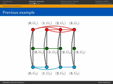
Theoretical introduction
Previous example
0 1 2 3
0 1 2 3
0 1 2 3
Multiplex network inference Petar Veličković
Introduction Multiplex networks Hidden Markov Models Multiplex HMMs
Theoretical introduction
Previous example
(0, G3) (1, G3) (2, G3) (3, G3)
(0, G2) (1, G2) (2, G2) (3, G2)
(0, G1) (1, G1) (2, G1) (3, G1)
Multiplex network inference Petar Veličković

Introduction Multiplex networks Hidden Markov Models Multiplex HMMs
Theoretical introduction
We have a multiplex network!
Multiplex network inference Petar Veličković

Introduction Multiplex networks Hidden Markov Models Multiplex HMMs
Review of applications
Examples
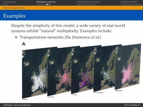
Despite the simplicity of this model, a wide variety of real-world
systems exhibit “natural” multiplexity. Examples include:
I Transportation networks (De Domenico et al.)
Multiplex network inference Petar Veličković
Introduction Multiplex networks Hidden Markov Models Multiplex HMMs
Review of applications
Examples
Despite the simplicity of this model, a wide variety of real-world
systems exhibit “natural” multiplexity. Examples include:
I Transportation networks (De Domenico et al.)
Multiplex network inference Petar Veličković

Introduction Multiplex networks Hidden Markov Models Multiplex HMMs
Review of applications
Examples
Despite the simplicity of this model, a wide variety of real-world
systems exhibit “natural” multiplexity. Examples include:
I Genetic networks (De Domenico et al.)
Multiplex network inference Petar Veličković

Introduction Multiplex networks Hidden Markov Models Multiplex HMMs
Review of applications
Examples
Despite the simplicity of this model, a wide variety of real-world
systems exhibit “natural” multiplexity. Examples include:
I Social networks (Granell et al.)
Multiplex network inference Petar Veličković

Introduction Multiplex networks Hidden Markov Models Multiplex HMMs
Theoretical introduction
Markov chains
I Let S be a discrete set of states, and {Xn}n≥0 a sequence of
random variables taking values from S.
I This sequence satisfies the Markov property if it is
memoryless: if the next value in the sequence depends only on
the current value; i.e. for all n ≥ 0:
P(Xn+1 = xn+1|Xn = xn, . . . , X0 = x0)
= P(Xn+1 = xn+1|Xn = xn)
It is then called a Markov chain.
I Xt = xt signifies that the chain is in state xt (∈ S) at time t.
Multiplex network inference Petar Veličković
Introduction Multiplex networks Hidden Markov Models Multiplex HMMs
Theoretical introduction
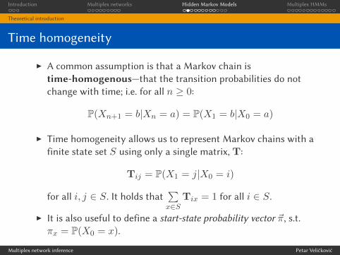
Time homogeneity
I A common assumption is that a Markov chain is
time-homogenous—that the transition probabilities do not
change with time; i.e. for all n ≥ 0:
P(Xn+1 = b|Xn = a) = P(X1 = b|X0 = a)
I Time homogeneity allows us to represent Markov chains with a
finite state set S using only a single matrix, T:
Tij = P(X1 = j|X0 = i)
for all i, j ∈ S. It holds that
∑x∈S
Tix = 1 for all i ∈ S.
I It is also useful to define a start-state probability vector ~π, s.t.
πx = P(X0 = x).
Multiplex network inference Petar Veličković

Introduction Multiplex networks Hidden Markov Models Multiplex HMMs
Theoretical introduction
Markov chain example
x
y
z
1
0.5
0.5
0.7
0.3
S = {x, y, z}
T =
0.0 1.0 0.00.0 0.5 0.50.3 0.7 0.0
Multiplex network inference Petar Veličković

Introduction Multiplex networks Hidden Markov Models Multiplex HMMs
Theoretical introduction
Hidden Markov Models
I A hidden Markov model (HMM) is a Markov chain in which
the state sequence may be unobservable (hidden).
I This means that, while the Markov chain parameters (e.g.
transition matrix and start-state probabilities) are still known,
there is no way to directly determine the state sequence
{Xn}n≥0 the system will follow.
I What can be observed is an output sequence produced at each
time step, {Yn}n≥0. The output sequence can assume any
value from a given set of outputs, O.
I Here we will assume O to be discrete, but it is easily extendable
to the continuous case (GMHMMs, as used in the paper) and
all the standard algorithms retain their usual form.
Multiplex network inference Petar Veličković

Introduction Multiplex networks Hidden Markov Models Multiplex HMMs
Theoretical introduction
Further parameters
I It is assumed that the output at any given moment depends
only on the current state; i.e. for all n ≥ 0:
P(Yn = yn|Xn = xn, ..., X0 = x0, Yn−1 = yn−1, ..., Y0 = y0)
=P(Yn = yn|Xn = xn)
I Assuming time homogeneity on P(Yn = yn|Xn = xn) as
before, the only additional parameter needed to fully specify
an HMM is the output probability matrix, O, defined as
Oxy = P(Y0 = y|X0 = x)
Multiplex network inference Petar Veličković
Introduction Multiplex networks Hidden Markov Models Multiplex HMMs
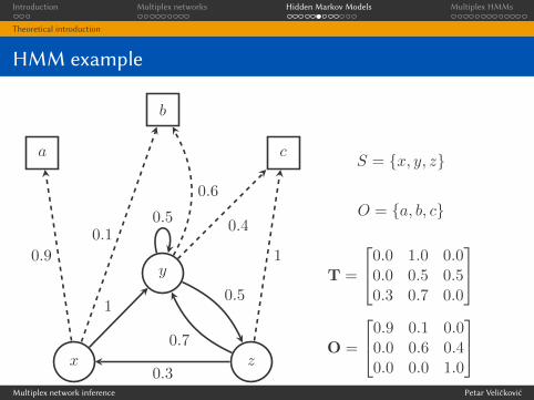
Theoretical introduction
HMM example
x
y
z
a
b
c
1
0.5
0.5
0.7
0.3
0.9
0.1
0.6
0.4
1
S = {x, y, z}
O = {a, b, c}
T =
0.0 1.0 0.00.0 0.5 0.50.3 0.7 0.0
O =
0.9 0.1 0.00.0 0.6 0.40.0 0.0 1.0
Multiplex network inference Petar Veličković
Introduction Multiplex networks Hidden Markov Models Multiplex HMMs
Theoretical introduction
Learning and inference
There are three main problems that one may wish to solve on a
(GM)HMM, and each can be addressed by a standard algorithm:
I Probability of an observed output sequence. Given an output
sequence, {yt}Tt=0, determine the probability that it was
produced by the given HMM Θ, i.e.
P(Y0 = y0, . . . , YT = yT |Θ) (1)
This problem is e�iciently solved with the forward algorithm.
Multiplex network inference Petar Veličković

Introduction Multiplex networks Hidden Markov Models Multiplex HMMs
Theoretical introduction
Learning and inference
There are three main problems that one may wish to solve on a
(GM)HMM, and each can be addressed by a standard algorithm:
I Most likely sequence of states for an observed output sequence.Given an output sequence, {yt}Tt=0, determine the most likely
sequence of states, {x̂t}Tt=0, that produced it within a given
HMM Θ, i.e.
{x̂t}Tt=0 = argmax{xt}Tt=0
P({xt}Tt=0|{yt}Tt=0,Θ) (2)
This problem is e�iciently solved with the Viterbi algorithm.
Multiplex network inference Petar Veličković

Introduction Multiplex networks Hidden Markov Models Multiplex HMMs
Theoretical introduction
Learning and inference
There are three main problems that one may wish to solve on a
(GM)HMM, and each can be addressed by a standard algorithm:
I Adjusting the model parameters. Given an output sequence,
{yt}Tt=0 and an HMM Θ, produce a new HMM Θ′ that is more
likely to produce that sequence, i.e.
P({yt}Tt=0|Θ′) ≥ P({yt}Tt=0|Θ) (3)
This problem is e�iciently solved with the Baum-WelchAlgorithm.
Multiplex network inference Petar Veličković

Introduction Multiplex networks Hidden Markov Models Multiplex HMMs
Problem setup
Supervised learning
I One of the most common kinds of machine learning is
supervised learning; the task is to construct a learning algorithmthat will, upon observing a set of data with known labels
(training data), construct a function capable of determining
labels for, thus far, unseen data (test data).
Learning algorithm, L
Labelling function, h
Training data, ~s
Unseen data, x Label, y
L(~s)
h(x)
Multiplex network inference Petar Veličković

Introduction Multiplex networks Hidden Markov Models Multiplex HMMs
Problem setup
Binary classification
I The simplest example of a problem solvable via supervised
learning is binary classification: given two classes (C1 and C2)
determining which class an input x belongs to.
I The applications of this are widespread:
I Diagnostics (does a patient have a given disease, based on
glucose levels, blood pressure, and sim. measurements?);
I Giving credit (is a person expected to return their credit, based
on their financial history?);
I Trading (should a stock be bought or sold, depending on
previous price movements?);
I Autonomous driving (are the driving conditions too dangerous
for self-driving, based on meteorological data?);
I . . .
Multiplex network inference Petar Veličković
Introduction Multiplex networks Hidden Markov Models Multiplex HMMs
Classification via HMMs
Classification via HMMs
I The training data consists of sequences for which class
membership (in C1 or C2) is known.
I We may construct two separate HMMs; one producing all the
training sequences belonging to C1, the other producing all the
training sequences belonging to C2. The models can be trained
by doing a su�icient number of iterations of the Baum-Welchalgorithm over the sequences from the training data belonging
to their respective classes.
I A�er constructing the models, classifying new sequences is
simple; employ the forward algorithm to determine whether it
is more likely that a new sequence was produced by C1 or C2.
Multiplex network inference Petar Veličković

Introduction Multiplex networks Hidden Markov Models Multiplex HMMs
Motivation
A slightly di�erent problem
I Now assume that we have access to more than one output type
at all times (e.g. if we measure patient parameters through
time, we may simultaneously measure the blood pressure and
blood glucose levels).
I We may a�empt to reformulate our output matrix O, such that
it has k + 1 dimensions for k output types:
Ox,a,b,c,... = P (a, b, c, . . . |x)
. . . however this becomes intractable fairly quickly, both
memory and numerics-wise. . . also, many combinations of the
outputs may never be seen in the training data.
Multiplex network inference Petar Veličković

Introduction Multiplex networks Hidden Markov Models Multiplex HMMs
Motivation
Modelling
I There exists a variety of ways for handling multiple outputs
simultaneously, however most of them do not take into
account the potentially nontrivial nature of interactions
between these outputs.
I Worst o�ender: Naïve/Idiot Bayes
I This is where multiplex networks come into play, as a model
which was proved e�icient in modelling real-world systems.
I Fundamental idea: We will model each of the outputsseparately within separate HMMs, a�er which we will combine
the HMMs into a, larger-scale, multiplex HMM. The entire
structure will still behave as an HMM, so we will be able to
classify using the forward algorithm, just as before.
Multiplex network inference Petar Veličković

Introduction Multiplex networks Hidden Markov Models Multiplex HMMs
Model description
Interlayer edges
I Therefore, we assume that we have k HMMs (one for each
output type) with n nodes each.
I In each time step, the system is within one of the nodes of one
of the HMMs, and may either:
I change the current node (remaining within the same HMM), or
I change the current HMM (remaining in the same node).
I Assumption: the multiplex is layer-coupled the probabilities of
changing the HMM at each timestep can be represented with a
single matrix, ω (of size k × k).
I Therefore, ωij gives the probability of, at any time step,
transitioning from the HMM producing the ith output type to
the HMM producing the jth output type.
Multiplex network inference Petar Veličković

Introduction Multiplex networks Hidden Markov Models Multiplex HMMs
Model description
Multiplex HMM parameters
I Important: while in the ith HMM, we are only interested in
the probability of producing the ith output type; we do notconsider the other k − 1 types! (they are assumed to be producedwith probability 1)
I With that in mind, the full system may be observed as an
HMM over node-layer pairs (x, i), such that:
π(x,i) = ωiiπix
T(a,i),(b,j) =
0 a 6= b ∧ i 6= j
ωij a = b ∧ i 6= j
ωiiTiab i = j
O(x,i),~y = Oixyi
Multiplex network inference Petar Veličković
Introduction Multiplex networks Hidden Markov Models Multiplex HMMs
Model description
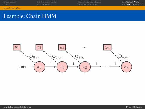
Example: Chain HMM
x0start x1 x2 . . . xn1 1 1 1
y0 y1 y2 . . . yn
O0,y0 O1,y1 O2,y2 On,yn
Multiplex network inference Petar Veličković

Introduction Multiplex networks Hidden Markov Models Multiplex HMMs
Model description
Example: Two Chain HMMs
x0start x1 x2 . . . xn1 1 1 1
y0 y1 y2 . . . yn
O0,y0 O1,y1 O2,y2 On,yn
x0start x1 x2 . . . xn1 1 1 1
y′0 y′1 y′2 . . . y′n
O′0,y′0 O′1,y′1 O′2,y′2 O′n,y′n
Multiplex network inference Petar Veličković
Introduction Multiplex networks Hidden Markov Models Multiplex HMMs
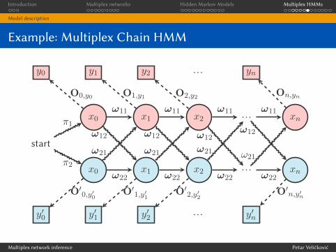
Model description
Example: Multiplex Chain HMM
x0 x1 x2 . . . xnω11 ω11 ω11 ω11
y0 y1 y2 . . . yn
O0,y0 O1,y1 O2,y2 On,yn
x0 x1 x2 . . . xnω22 ω22 ω22 ω22
y′0 y′1 y′2 . . . y′n
O′0,y′0 O′1,y′1 O′2,y′2 O′n,y′n
ω12 ω12 ω12ω12
ω21 ω21 ω21 ω21
start
π1
π2
Multiplex network inference Petar Veličković

Introduction Multiplex networks Hidden Markov Models Multiplex HMMs
Training and classification
Training
I Training the individual HMM layers (i.e. determining the
parameters ~πi,Ti,Oi) may be done as before (by using the
Baum-Welch algorithm).
I Determining the entries of ω is much harder; this matrix
specifies the relative dependencies between processes
generating the di�erent output types, which is undetermined
for many practical problems!
I Therefore we assume an optimisation approach that makes no
further assumptions about the problem—within my project, a
multiobjective genetic algorithm, NSGA-II, was used to
determine optimal values of entries of ω.
Multiplex network inference Petar Veličković
Introduction Multiplex networks Hidden Markov Models Multiplex HMMs
Training and classification
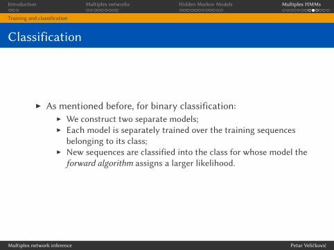
Classification
I As mentioned before, for binary classification:
I We construct two separate models;
I Each model is separately trained over the training sequences
belonging to its class;
I New sequences are classified into the class for whose model the
forward algorithm assigns a larger likelihood.
Multiplex network inference Petar Veličković

Introduction Multiplex networks Hidden Markov Models Multiplex HMMs
Training and classification
Pu�ing it all together
~sTraining set,
−−−−−−−→(t1, t2, . . . ) ∈ C1
−−−−−−−→(t1, t2, . . . ) ∈ C2
Train layer 1 Train layer 2 . . .
Train interlayer edges
Train layer 1 Train layer 2 . . .
Train interlayer edges
Baum-Welch
NSGA-II
Baum-Welch
NSGA-II
~yUnseen sequence,
forward alg. forward alg.P(~y|C1) P(~y|C2)
C = argmaxCiP(~y|Ci)
Multiplex network inference Petar Veličković

Introduction Multiplex networks Hidden Markov Models Multiplex HMMs
Results and implementation
Application & results
I My project has applied this method to classifying patients for
breast invasive carcinoma based on gene expression and
methylation data for genes assumed to be responsible: we have
achieved a mean accuracy of 94.2% and mean sensitivity of
95.8% a�er 10-fold crossvalidation!
I This was accomplished without any optimisation e�orts:I Fixed the number of nodes to n = 4;
I Used the standard NSGA-II parameters without tweaking;
I Ordered the sequences based on the euclidean norm of the
expression and methylation levels.
so we expect further advances to be possible.
Multiplex network inference Petar Veličković
Introduction Multiplex networks Hidden Markov Models Multiplex HMMs
Results and implementation
Implementation and conclusions
I You may find the full C++ implementation of this model at
https://github.com/PetarV-/muxstep.
I We are currently in the process of publishing a new paper
describing basic workflows with the so�ware.
I Hopefully, more multiplex-related work to come!
I Developed viral during the Hack Cambridge hackathon; check it
out at http://devpost.com/software/viral. . .
Multiplex network inference Petar Veličković

Introduction Multiplex networks Hidden Markov Models Multiplex HMMs
Results and implementation
Thank you!
�estions?
Multiplex network inference Petar Veličković