Using Hedonic Property Models to Value Public Water Bodies: A Note Regarding Specification Issues

by

Nicholas Z. Muller

October 2007

MIDDLEBURY COLLEGE ECONOMICS DISCUSSION PAPER NO. 07-21

DEPARTMENT OF ECONOMICS MIDDLEBURY COLLEGE

MIDDLEBURY, VERMONT 05753

http://www.middlebury.edu/~econ

Using Hedonic Property Models to Value Public Water Bodies: A Note Regarding Speci�cation

Issues.

Nicholas Z. MullerDepartment of EconomicsEnvironmental Studies ProgramMiddlebury CollegeMiddlebury, VT 05753nmuller@middlebury.edu802-443-5918July 6th, 2007

AbstractThe hedonic literature has established that public water bodies provide external bene�ts that are

re�ected in the value of nearby residential real estate. The literature has employed several approachesto quantify these nonmarket services. With a residential hedonic model, this paper tests whether modelspeci�cation a¤ects resource valuation using an actively managed reservoir in Indiana and a passivelymanaged lake in Connecticut. The results indicate that valuation is quite sensitive to model speci�cation,and that omitting either the waterview or waterfront variables from the hedonic function likely results in amisspeci�ced model. The �ndings from this study are important for researchers and public agencies chargedwith managing water resources to bear in mind as the external bene�ts from existing or proposed man-madelakes and reservoirs are estimated. Therefore, while it requires considerably more e¤ort to determine whichproperties are in waterfront loactions and which properties have a view, the potential misspeci�cation of"distance-only" models likely justi�es these extra research costs. Further, the �ndings in this analysis callinto question results from "distance-only" models in the literature.

AGU Index Terms: 6304 Bene�t-cost analysisKeywords: Hedonic Model, Public Water Bodies, Valuation

Acknowledgements: The author wishes to thank the Glaser Progress Foundation for funding this project.I would also like to thank Robert Mendelsohn, Nathaniel Keohane, and participants in the Yale EnvironmentalEconomics Seminar for their helpful comments.

2

1 Introduction

Economists using hedonic property models have established that public water bodies provide external bene�ts

that are re�ected in the value of nearby residential real estate. The literature has employed a number of

approaches to quantify these nonmarket services. Several studies have used distance to the water to measure

the nonmarket services generated by public water bodies [Mahan, Polasky, Adams, 2000]. Other authors

have controlled for both distance and view services [Brown, Pollakowski, 1977]. Another strategy measures

three distinct services: access (measured by distance to the water), a view of the water, and adjacency

[Lansford, Jones, 1995; Loomis, Feldman, 2003]. Since hedonic models are often used to value water bodies,

speci�cation is especially critical. Bias due to the omission of relevant variables a¤ects parameter estimates

in the regression function which, in turn, impacts valuation. This paper tests how amenity measurement

in�uences the bene�t estimates for public water bodies.

The importance of speci�cation is tested using the three approaches to amenity measurement outlined

above. Each model is used to value two public lakes. Along with a standard assortment of structural,

economic and neighborhood variables, the �rst model employs only distance to value the lakes. The second

model includes both distance and water view, and the third model uses distance, water view and waterfront

regressors to measure the services produced by the lakes. This experimental design facilitates an assessment

of how speci�cation, through amenity measurement, a¤ects valuation. A Hausman test [Hausman, 1978] is

used to test whether distance to the water is an endogenous variable when the water view and the waterfront

variables are omitted from the hedonic model. Further, the Hausman test is used to test whether water view

is endogenous when the waterfront control is omitted.

The data consist of sales from housing markets surrounding two lakes; Lake Monroe, an actively managed

Army Corps of Engineers reservoir in Indiana, and Candlewood Lake, a passively managed lake in Connecticut.

Lake Monroe is managed for �ood control, and as a source of irrigation and drinking water. Management

strategies dictate dramatic seasonal �uctuations in water levels. In contrast, Candlewood Lake is predominantly

a recreation resource which does not experience drastic �uctuations in water levels. The hedonic models are

applied to each sample separately.

This empirical setting also addresses an interesting management issue raised by Loomis and Feldman

[2003] and Lansford and Jones [1995]. These authors indicate that anthropogenic reductions in lake levels

constitute a signi�cant disamenity, negatively a¤ecting housing prices. This �nding has important implications

for cost bene�t analyses of lakes managed for irrigation and hydroelectricity production. Although this

analysis does not directly estimate the implicit price of water levels, I qualitatively test this hypothesis in

the following manner. Fluctuations in water levels likely have the most tangible market implications for

1

waterfront properties. Therefore, if water levels do a¤ect the price of such homes, one would expect to

observe a di¤erence in the waterfront premium a¢ xed to properties on Candlewood Lake, which has a stable

water level, and Lake Monroe which experiences substantial seasonal lake level changes. In the current

setting, a signi�cantly smaller premium for waterfront houses on Lake Monroe would provide qualitative

support for the hypothesis that active lake management a¤ects the amenity value of lakes.

The results indicate that valuation is quite sensitive to model speci�cation. Using the Lake Monroe

sample, the distance-only model produces an annual amenity value that is 40% greater than that produced

when controlling for view and adjacency. Using the Candlewood Lake sample, the total value generated by

the distance-only model is 25% greater than the total amenity value produced when controlling for view

and adjacency. The di¤erence in total lake values is driven by the parameter estimate for distance to the

lake: in both samples this coe¢ cient declines precipitously when view and adjacency are added to the

distance-only model. The Hausman test provides strong evidence that lake distance is endogenous when the

view and waterfront controls are omitted from the hedonic price function. Taken together, it is likely that

the lake distance coe¢ cient su¤ers from omitted variable bias in distance-only models. The strong e¤ect

that this bias bears upon the total value of the lakes suggests that the application of distance-only models

to estimate external bene�ts generated by public water bodies is quite problematic. Finally, waterfront and

access services are generated by the passively managed, Candlewood Lake. In contrast, only view and access

services are provided by Lake Monroe, the reservoir. This resource does not generate waterfront services.

This may suggest that �uctuations in water levels due to management practices produces a signi�cant

disamenity for waterfront homeowners.

2 Methods

2.1 Model Speci�cation

The econometric framework is built upon a log-linear hedonic model. This speci�cation was chosen for a

number of reasons. First, imposing a linear form on the hedonic function implies, undesirably, that perfect

repackaging of property characteristics is possible [Freeman, 2003]. Second, the hedonic models employ

proxy variables and Cropper, Deck and McConnell [1988] suggest that linear and log-linear functional forms

outperform other forms when proxy measurements are employed. Third, since the estimated regression

functions are used to generate amenity values, it is preferable to maintain a relatively simple form. Employing

more complicated functional forms impedes both interpretation of the parameter estimates and their use

in valuation. Finally, preliminary regression results indicated that the log-linear form exhibited an excellent

2

�t to the data. The full list of variables included in the regression models is shown in table 1. Descriptive

statistics are shown in tables 2 and 3.

Using the log-linear form, the empirics begin with the most parsimonious speci�cation found in the

literature. The benchmark strategy, model (1), employs the distance to the water (D) as the solitary amenity

measure in the hedonic price function. Mahan, Polasky, and Adams [2000] employed the distance-only model

to value urban wetlands. Model (2) controls for view services (V ) and distance. Brown and Pollakowski

[1977] used this approach to value shoreline. Model (3) incorporates adjacency (F ), view, and distance.

This speci�cation stems from the work of Lansford and Jones [1995] and Loomis and Feldman [2003]. In a

departure from the literature, this study uses a more �exible functional form for proximity; models (1,2,3)

are estimated employing cubic splines to capture the relationship between proximity and price. The m�(D)

notation represents the spline function.

This experimental design tests the implications of speci�cation, through environmental amenity measurement,

for valuation. Since the structural, economic and neighborhood controls are the same in each model, the

di¤erences in values produced each model are directly attributable to the di¤erent amenity measurement

strategies.

log(Pi) = �0 + �1Xi + �2Ni +m�(Di) + "i (1)

where: �0; :::; �n; � Statistically Estimated ParametersXi Physical/structural characteristics property (i)N Neighborhood characteristicsD Straight-Line Distance to Nearest Shore PointP sales price ($2000)" error term

log(Pi) = �0 + �1Xi + �2Ni +m�(Di) + �4Vi + "i (2)

where: V Water view Binary

log(Pi) = �0 + �1Xi + �2Ni +m�(Di) + �4Vi + �5Fi + "i (3)

where: F Water front Binary

Although none of the above models address the necessarily ad hoc nature of the hedonic property model,

prior to estimation there is reason to believe that model (3) embodies the preferable approach. First, the

goal in the hedonic function is to use an amenity measurement that mimics consumers�perceptions of the

3

amount of the amenity embodied in each property [Freeman, 2003]. Of the models found in the literature,

model (3) is the most e¤ective at capturing the criteria that consumers use when ranking and evaluating

residential properties close to a public water body. These criteria are evident in how realtors advertise such

properties: waterfront homes, homes with a water view, and homes a number of blocks from the water.

Omitting any of these attributes reduces the correspondence between amenity measurement in the hedonic

function and the criteria used by consumers.

Model (3) is also preferable because of the clear potential for measurement error in models (1) and (2).

In model (1), distance to the water presumably captures the bundle of water-related services embodied in

each property. In model (2) view likely captures the price e¤ects of both view and adjacency services since

the view and (omitted) adjacency variables are likely to be highly correlated. In this setting, the role of

distance changes. This variable now captures the e¤ect which the degree of access to the water bears upon

housing prices. Model (3) eliminates this imprecision by including explicit controls for each of these three

services.

The non-parametric approach to modeling the relationship between distance to the lakes and housing

prices using cubic splines requires determining the appropriate smoothing parameter (�); which controls the

number of knots (in�ection points) in the spline function. This analysis uses a data-driven mechanism in

order to select an appropriate value for (�). Speci�cally, a variety of degrees of smoothness for the spline

function are tested and the �t of each is evaluated using the leave-one-out-method (Hardle, 1990; Stone,

1974). The mean square error (MSE) is estimated for each sample.

MSE =1

n

nXi=1

�Pi � P̂i

�2(4)

where: Pi observed sale price of property (i).

P̂i model prediction of sale price for property (i).

The value of (�) that minimizes the MSE is selected as the preferred smoothing parameter for the

econometric and valuation experiments. The optimal (error-minimizing) smoothing parameter is permitted

to vary between the two samples.

For the remaining portions of this paper, values stemming from the distance to the water variable are referred to as accessservices.

4

2.2 Valuation Methodology

The hedonic literature has explored using estimated hedonic property models to determine the welfare

e¤ects of changes in environmental quality [Freeman, 2003; Palmquist, 1992]. Using the log-linear functional

form, the marginal willingness-to-pay (MWTP) for the environmental amenity is equivalent to the regression

coe¢ cient corresponding to the amenity (�) times the price (P), [Loomis, Feldman, 2003].

MWTP = P � � (5)

However, Freeman [2003] and others have discussed the di¢ culties involved with using the implicit

prices estimated in hedonic property models to compute welfare e¤ects for non-marginal changes in an

environmental amenity. In this study, there are two types of environmental changes that a¤ect the value

of residential real estate. Variation in the distance between properties and the water body is a continuous

function, so small relocations along the distance gradient may be viewed as marginal changes. In contrast,

the waterview and waterfront categories are discrete categories; either a property is adjacent to the water or

it is not. Movement of a property into and out of this category is clearly a non-marginal change. Therefore,

in light of Freeman [2003], attempting to assess the welfare implications of the waterfront and water view

amenities using implicit prices is problematic.

However, Palmquist [1992] points out that if the number of properties a¤ected by an amenity is small

relative to a larger real estate market, then the hedonic price function does not shift for non-marginal

changes in the amenity. In this case, the change in price associated with changes to the amenity is correctly

interpreted as a welfare measurement. This approach also requires the assumption of low moving costs. In

each sample, this study focuses on roughly 300 properties within larger real estate markets. The assumptions

embodied in the work of Palmquist [1992] are invoked in order to use the methods outlined above to compute

the aggregate welfare e¤ect of the lakes in this study.

In order to convert the market prices, which represent the present value of a stream of rental income, to

the more conventional welfare measure of annualized bene�ts, Freeman [2003] points out that the following

calculations are necessary. Using (r) the social rate of return on investment, and (t) the local property

tax rate, and the housing price (Pi), annualized rental value of property (i), denoted (Ri) is equivalent to

equation (6).

The Lake Monroe sample is situated within the Bloomington, Indiana market. This city contains 26,000 households.Similarly, the Candlewood Lake sample is nested within both the New Milford and New Fair�eld markets; these towns contain15,000 households. Clearly the number of properties a¤ected by these two amenities is quite small relative to each residentialreal estate market.

5

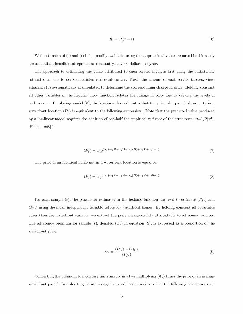
Ri = Pi(r + t) (6)

With estimates of (t) and (r) being readily available, using this approach all values reported in this study

are annualized bene�ts; interpreted as constant year-2000 dollars per year.

The approach to estimating the value attributed to each service involves �rst using the statistically

estimated models to derive predicted real estate prices. Next, the amount of each service (access, view,

adjacency) is systematically manipulated to determine the corresponding change in price. Holding constant

all other variables in the hedonic price function isolates the change in price due to varying the levels of

each service. Employing model (3), the log-linear form dictates that the price of a parcel of property in a

waterfront location (Pf ) is equivalent to the following expression. (Note that the predicted value produced

by a log-linear model requires the addition of one-half the empirical variance of the error term: �=1=2(s2);

[Heien, 1968].)

(Pf ) = exp(�0+�1X+�2N+m�(D)+�4V+�51+�) (7)

The price of an identical home not in a waterfront location is equal to:

(P0) = exp(�0+�1X+�2N+m�(D)+�4V+�50+�) (8)

For each sample (s), the parameter estimates in the hedonic function are used to estimate (Pfs) and

(P0s) using the mean independent variable values for waterfront homes. By holding constant all covariates

other than the waterfront variable, we extract the price change strictly attributable to adjacency services.

The adjacency premium for sample (s), denoted (�s) in equation (9); is expressed as a proportion of the

waterfront price.

�s =(Pfs)� (P0s)

(Pfs)(9)

Converting the premium to monetary units simply involves multiplying (�s) times the price of an average

waterfront parcel. In order to generate an aggregate adjacency service value, the following calculations are

6

necessary. First, the housing density in each sample area, denoted (Ds), is determined using U.S. Census

data (U.S. Census, 2006). Next, the total number of homes in waterfront locations (Hfs) is determined by

multiplying the sample housing density (Ds) by the land area in water front zones (Afs), (see appendix A.2).

Hfs = (Ds)� (Afs) (10)

The aggregate value of waterfront services for each sample (WFs) is found by multiplying the observed

average price of a waterfront home��Pfs�by the number of homes in waterfront locations (Hfs ) and by the

estimated waterfront premium (�s).

WFs = (Hfs)� ( �Pfs)� (�s) (11)

The valuation procedure for view services proceeds in an analogous manner. The estimation of aggregate

access values relies on a slightly di¤erent approach than that used for adjacency and view values. Valuing

access services requires �rst determining the distance at which the water bodies�in�uence on housing prices

diminishes. In order to determine the boundary of each lake�s e¤ect on housing prices, the spline model

�tted to the lake distance variable, m�(D), is examined for a local minimum point. Using the Lake Monroe

sample, the m�(D) function minimizes at 1.8 miles from the lake: this point is used as the boundary of the

lake�s in�uence on property values. Using the Connecticut sample, the �tted spline model, m�(D), minimizes

at 1.7 miles from the lake. This point is used as the boundary of the lake�s in�uence on property values for

the non-parametric models applied to the Connecticut sample.

For each sample, the number of homes in the zone from the lakeshore to the sample-speci�c boundary

points (1.7 and 1.8 miles) is estimated. This necessitates determining the total land area in this lake-in�uenced

zone and multiplying the area times the observed housing density (U.S. Census, 2006). The number of homes

in the land area corresponding to sample (s) is denoted (Hs).

Then the estimated regression models are used to predict the mean price (Pms) for properties in each

sample, excluding properties beyond the boundary points in each sample. This entails inserting the mean

values for each covariate, from the spatially restricted samples, into the estimated model. Next, the boundary

price is generated by inserting the boundary distance into the estimated regression model, while all other

independent variables are held at their mean levels. This isolates the price e¤ect of relocating a property

from the mean distance to the boundary distance. The access premia (s) are calculated by subtracting the

7

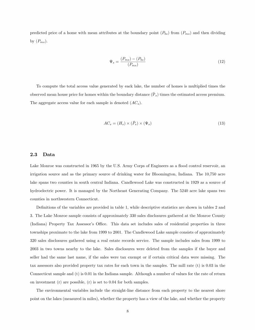
predicted price of a home with mean attributes at the boundary point (Pbs) from (Pms) and then dividing

by (Pms).

s =(Pms)� (Pbs)

(Pms)(12)

To compute the total access value generated by eack lake, the number of homes is multiplied times the

observed mean house price for homes within the boundary distance (P̄s) times the estimated access premium.

The aggregate access value for each sample is denoted (ACs).

ACs = (Hs)� ( �Ps)� (s) (13)

2.3 Data

Lake Monroe was constructed in 1965 by the U.S. Army Corps of Engineers as a �ood control reservoir, an

irrigation source and as the primary source of drinking water for Bloomington, Indiana. The 10,750 acre

lake spans two counties in south central Indiana. Candlewood Lake was constructed in 1929 as a source of

hydroelectric power. It is managed by the Northeast Generating Company. The 5240 acre lake spans two

counties in northwestern Connecticut.

De�nitions of the variables are provided in table 1, while descriptive statistics are shown in tables 2 and

3. The Lake Monroe sample consists of approximately 330 sales disclosures gathered at the Monroe County

(Indiana) Property Tax Assessor�s O¢ ce. This data set includes sales of residential properties in three

townships proximate to the lake from 1999 to 2001. The Candlewood Lake sample consists of approximately

320 sales disclosures gathered using a real estate records service. The sample includes sales from 1999 to

2003 in two towns nearby to the lake. Sales disclosures were deleted from the samples if the buyer and

seller had the same last name, if the sales were tax exempt or if certain critical data were missing. The

tax assessors also provided property tax rates for each town in the samples. The mill rate (t) is 0.03 in the

Connecticut sample and (t) is 0.01 in the Indiana sample. Although a number of values for the rate of return

on investment (r) are possible, (r) is set to 0.04 for both samples.

The environmental variables include the straight-line distance from each property to the nearest shore

point on the lakes (measured in miles), whether the property has a view of the lake, and whether the property

8

is adjacent to the lakeshore. All properties in each sample were visited in order to determine if the property

is adjacent to the lake or if it has a view of the lake. The properties were visited during the summer months,

so it is likely that certain properties that do not have summertime views have a view in the winter when the

predominantly deciduous trees in each study area lose their leaves.

The dependent variable is the natural log of the sales price adjusted to $2000. In models (1), (2), and

(3) the physical and structural characteristics include; acreage of the lot, living area in the structure, and

number of stories in the structure. This approach relies on the living area of each structure as a proxy

for more detailed structural characteristics such as the number of bedrooms, bathrooms, and �replaces.

Brookshire et al. [1982] employ this approach. The Lake Monroe sample includes condominiums, mobile

homes and single-family houses. Therefore, the models applied to that sample include dummy variables for

condominiums and mobile homes. Single-family homes are the default case. In the Candlewood Lake sample

all observations are single-family houses. The inclusion of these particular house and property attributes is

rooted in previous residential hedonic models [Brown, Pollakowski, 1977; Earnhart, 2001; Mahan, Polasky,

Adams, 2000].

The vector of neighborhood characteristics includes distance to the nearest town in both linear and

quadratic forms. Both samples include measurements of the year in which the sale occurred. The year of

sale variables are included as a proxy measurement for temporal changes in each local housing market. In

particular, these variables are intended to capture annual variation associated with property tax assessments

and property tax rates; both of which have clear implications for housing prices. Since these are binary

variables it necessary to omit one of the year of sale variables from the models. The 2001 variable is omitted

from the models. Further, the annual average prime rate is included as a proxy variable for mortgage interest

rates and annual GDP is included to proxy for aggregate income. Structure age data was only available for

the Candlewood Lake sample. In the Lake Monroe sample, properties were drawn from three townships

and two elementary school districts. The Candlewood Lake sample contains properties in two towns. In

both cases, these geographic distinctions function as proxy measurements for neighborhood and community

characteristics.

3 Results

3.1 Econometrics

Table 4 displays the regression results for both samples. The column headings indicate the sample and

the model speci�cation (shown in parentheses). All regression analyses were conducted using ordinary least

9

squares with heteroskedasticity-robust standard errors, [White, 1990]. While included in the models, the

covariates that were consistently not signi�cant at � = 0:10 are omitted from Table 2. In each of the

models, the covariates measuring the structural aspects of the properties behave as intuition would predict.

The positive impact which lot size and the size of the structure have on price are notable examples of this

conformity. This lends a degree of credibility to the models that is desirable given the use of the regression

coe¢ cients to value the non-market services produced by the lakes.

The most notable econometric result is the di¤erence in the mix of services produced by each lake. Using

model (3), adjacency and access services are produced by the passively managed Candlewood Lake. View

services are marginally signi�cant. View and access, but not adjacency, are produced by Lake Monroe, the

reservoir. The coe¢ cient associated with adjacency in the Candlewood Lake sample is approximately 0.61.

Thus, the price of a home adjacent to the lake is approximately 60% greater than an equivalent home not in

a waterfront location. Although marginally signi�cant, the view coe¢ cient is 0.07: this implies that a view

of the lake increases a property�s value by 7% above an equal property without a view. There is no premium

a¢ xed to waterfront properties in the Lake Monroe sample. Another important econometric result evident

in table 4 is that the �rst segment of the spline function, m�(D1), measuring distance to the water is negative

and statistically signi�cant in each model applied to both samples. Intuitively, this implies a premium for

properties located close to the lakes. However, the magnitude of the coe¢ cient corresponding to the �rst

spline segment is quite sensitive to model speci�cation. In both samples, the coe¢ cient corresponding to

the �rst spline segment is largest in model (1). Comparing model (1) to model (2) applied to the Lake

Monroe sample, this coe¢ cient declines from 0.26 to 0.15: a 40% reduction. Employing the Candlewood

Lake sample, again comparing model (1) to model (2), the coe¢ cient on the �rst spline segment drops from

0.18 to 0.08, a 55% decline. The decrease in the lake-distance coe¢ cient when the view control is added

to the model suggests that the measurement of distance to the water is capturing view services when the

waterview variable is omitted in model (1).

Using the Lake Monroe sample, adding the adjacency control causes no change to the coe¢ cients a¢ xed

to water view or lake distance in model (2). In contrast, employing the Candlewood Lake sample, adding the

adjacency regressor reduces the view coe¢ cient estimated using model (2) from 0.30, signi�cant at � = 0:01;

to 0.07 approaching signi�cance at � = 0:10. The reduction in the view coe¢ cient when the waterfront

variable is added indicates that the view variable is capturing waterfront services in model (2). The marked

sensitivity of the coe¢ cients for distance to the water in both samples and water view in the Connecticut

sample evident in table 4 are both strongly suggestive that model (1) and (2) are misspeci�ed. A Hausman

test is used to test for evidence of endogeneity in these regressors in models (1) and (2).

The results of the Hausman test are shown in table 5. Signi�cant t-statistics indicate evidence of

10

engodeneity for the variable shown in the right-hand column of table 5. Hence, it is clear that when used

solitarily, in model (1), the lake distance variable is endogenous in both samples. The Hausman test reveals

that using distance to the lake as the only amenity measurement in the hedonic function likely results in a

misspeci�ed model. This result meshes with the changes in the magnitude of the lake distance coe¢ cient

between models (1) and (2) observed in table 4. The signi�cant decrease in the size of the distance coe¢ cient

suggests that in model (1) lake distance captures some portion of view and adjacency services which are

omitted from model (1).

When model (2) is employed, the Hausman test reveals evidence that the view covariate is endogenous only

using the Candlewood Lake sample. So, the Hausman test indicates that model (2) is likely to be misspeci�ed

when using this sample. This result meshes with the decrease in the magnitude and the signi�cance of the

view coe¢ cient upon adding the control for adjacency services. This signi�cant reduction suggests that in

model (2) view captures some portion of adjacency services which are omitted from model (2). This holds

only for the Candlewood Lake sample. The following general �nding emerges from the Hausman test; the

coe¢ cients corresponding to the variables which the Hausman test indicates are likely endogenous are biased

upwards. The remaining question is to explore how this bias a¤ects valuation.

3.2 Valuation

Table 6 displays the valuation methodology as it is applied to model (3). Recall that the mill rate (t) is 0.03

in the Connecticut sample and (t) is 0.01 in the Indiana sample. The rate of return on investment (r) is set

to 0.04 for both samples. To compute the annual value derived from access services from Lake Monroe, the

method involves multiplying the annualized value of a property with average characteristics (all independent

variables except distance to the lake are set to the sample mean values), which in this case is $130,000 times

(r+t = 0.05), times the access premium of 0.19. This yields an annual value of access services for an average

property of $1235. Then, since there are 1710 homes within 1.8 miles of the lake, the per unit premium is

mutliplied times 1710 yielding an estimate of total annual access services of $2.0 million. This procedure is

repeated for each service in each model and for both samples. Table 7 displays the valuation results derived

from the application of these methods to all of the estimated models.

Employing model (1), the total lake values are $15.6 million and $4.6 million attributed to Candlewood

and Monroe lakes, respectively. On a per (property) unit basis, the total lake values are $5270 and $2700

(again for Candlewood and Monroe lakes, respectively). When the view covariate is added to model (1),

the total amenity value of both lakes declines signi�cantly: employing model (2) the values for Candlewood

and Monroe are $9.8 million and $2.8 million and the per unit values are $3310 and $1640, respectively. The

11

total amenity value attributed to both lakes drops by roughly 40%. In both samples, the decrease in total

amenity values is driven by the change in the magnitude of the e¤ect that access services have on sales prices.

Recall that adding the view control to model (1) reduced the magnitude of the e¤ect that proximity to the

lakes has on the price of property. This is clearly re�ected in the di¤erence in access services estimated using

model (1) compared to model (2): access services decline by 46% in the Indiana sample, and by 50% in the

Connecticut sample. Thus, the change in the parameter estimate for lake-distance has a dramatic e¤ect on

the total lake values.

Since the waterfront coe¢ cient is insigni�cant in model (3) applied to Lake Monroe, there is no change

to the total lake value when comparing the values predicted by model (2) and model (3): it remains $2.8

million. In contrast, the total amenity value derived from model (3) applied to the Candlewood Lake sample

is $11.7 million: this is 15% greater than the value derived from model (2) . Note that $11.7 million is

25% less than the value generated by model (1). In model (2), view services generate $2 million in value,

annually. Yet, when the waterfront variable is added in model (3), view services are e¤ectively $0 while

adjacency services are worth $2.5 million, annually. Recall from table 4 that adding the waterfront control

to model (2) dramatically reduced the e¤ect that a view of the lake has on the price of property: the view

coe¢ cient is 75% smaller and marginally signi�cant in model (3). Table 7 shows that the sensitivity of the

water view coe¢ cient to model speci�cation has a tangible impact on the total amenity values generated by

the two models.

The valuation results re�ect the �ndings discussed in section 3.1. Comparing model (1) to models (2)

and (3), table 4 shows that the distance coe¢ cient declines markedly when the other amenity variables

are added to the model. This suggests that the lake-distance coe¢ cient is biased upwards as this variable

captures the price e¤ects of view and adjacency which are omitted from model (1). Supporting the notion

that the distance parameter estimate is biased in model (1), is the Hausman test which provides evidence

that in model (1) the lake distance variable is endogenous in both samples. This in�uence of the sensitivity

of the distance coe¢ cient to model speci�cation is evident in table 7; using both samples, the access value

is substantially lower in model (2) and (3), after adding view and adjacency, than in model (1). A similar

issue Similarly, when comparing model (2) and (3) applied to the Connecticut sample, table 4 shows that in

model (2) the view coe¢ cient declines in magnitude and signi�cance when adjacency is added to the model.

It is likely that the view coe¢ cient is biased upward because the view variable captures the price e¤ect of

omitted adjacency services. As above, the Hausman test provides further evidence that the view covariate is

endogenous (in the Candlewood Lake sample). The e¤ect of the lake coe¢ cient on the total amenity value is

evident in table 7. First, the total values for Lake Monroe produced using models (2) and (3) are the same,

supporting the Hausman test �nding of no evidence of endogeneity when omitting adjacency from model

12

(2). However, comparing the service values for Candlewood Lake generated by models (2) and (3) reveals

evidence of this bias. That is, the value of view services is roughly $2 million in model (2) yet it is only $0

in model (3) when the waterfront variable is added to the hedonic function. Equally problematic is the fact

that the biased price for view services in model (2) underestimates the value of waterfront services estimated

using model (3). In sum, the valuation experiments reveal that the biased coe¢ cients, lake-distance in model

(1) and view in model (2), have tangible implications for valuation.

4 Conclusions

This paper �nds that how one measures the services provided by public water bodies in an hedonic price

function has a substantial impact on the total estimated value of the amenity. Evidence uncovered in this

study suggests that omitting controls for either view or adjacency services may result in misspecifation of the

hedonic price function. The implicit prices derived from hedonic models without such measurements may

be biased. Total amenity values estimated using such models will likely embody this bias. This analysis

indicates that such speci�cation errors may dramatically a¤ect valuation. This is important for researchers

and public agencies charged with managing water resources to bear in mind as the external bene�ts from

existing or proposed man-made lakes and reservoirs are estimated. Therefore, while it requires considerably

more e¤ort to determine which properties are in waterfront loactions and which properties have a view, the

potential misspeci�cation of "distance-only" models likely justi�es these extra research costs. Further, the

�ndings in this analysis call into question results from "distance-only" models in the literature.

The �ndings in this paper suggest that not all public water bodies provide adjacency services. Recall

that Candlewood Lake generates adjacency, view (which is marginally signi�cant), and access services

while Lake Monroe, the reservoir, provides only view and access services. Comparing the management

strategies employed on the lakes provides a plausible explanation for these results. Lake Monroe is a �ood

control reservoir, and a source of irrigation and drinking water which experiences management-induced

seasonal �uctuations in water levels. This likely has tangible implications for waterfront homeowners. For

instance, drastic reductions in water levels may present waterfront homeowners with considerable land area

normally underwater. In addition to impeding access, this area would likely possess undesirable qualities; no

vegetation, sunken debris, and o¤ensive odors. If consumers are aware of such conditions, this situation would

likely a¤ect the price of waterfront homes. In contrast, the management strategies applied to Candlewood

Lake do not involve drastic �uctuations in water levels. Instead, a rather constant water level is maintained.

In this more passive management setting, there is a substantial premium a¢ xed to waterfront locations.

Thus, intensive management necessitating unnatural �uctuations in water levels may impinge upon the �ow

13

of services to waterfront homeowners.

Prior studies provide quantitative evidence of this causal mechanism [Loomis, Feldman, 2003; Lansford,

Jones, 1995]. These authors estimate the e¤ect which reduced lake levels have on housing prices. In

both studies, the e¤ect is signi�cant and negative, indicating that reductions in lake levels constitute a

tangible disamenity. Further, in both articles, the observed �uctuations in lake levels are due to management

strategies much like those employed on Lake Monroe. Therefore, similarities between management techniques

employed at Lake Monroe and the lakes used in these prior studies points to anthropogenic �uctuations as

a likely contributing factor to the absence of a waterfront premium on Lake Monroe.

14

Table 1: Variable DescriptionsVariable Description

Price ($) Sales Price ($ 2000)Water Front 1 = Waterfront PropertyWater View 1 = Waterview PropertyDistance to Lake (mi) Straight-Line Distance from Property to Nearest Lake ShoreDistance to Town (mi) Straight-Line Distance from Property to Nearest Town CenterLot Size (Acres) Natural log of the acreage of the propertyLiving Area (ft2) Natural log of the square-footage of �nished living areaNumber of Stories Natural log of the total number of stories in structureAge of Structure Natural log of the age at time of saleNew Milford Twnshp 1 = in New Milford TownshipCondominium 1 = Unit is a CondominiumMobile Home 1 = Unit is a Mobile HomeClear Creek Township 1 = Unit is in Clear Creek TownshipPolk Township 1 = Unit is in Polk TownshipUnit Sold in 1999 1 = Unit was sold in 1999Unit Sold in 2000 1 = Unit was sold in 2000Unit Sold in 2002 1 = Unit was sold in 2002Unit Sold in 2003 1 = Unit was sold in 2003Elementary District 1 1 = Unit is in Elementary School District 1

15

Table 2: Descriptive Statistics Indiana Sample (n =329)Variable Mean Std. Dev. Min. Max.Price ($) 125,648 80,731.6 25,000 453,000Water Front 0.06 0.25 0 1Water View 0.24 0.43 0 1Distance to Lake (mi) 0.84 1.05 0.02 5.4Distance to Town (mi) 8.29 1.63 3.45 17Lot Size (Acres) 1.88 5.78 0.011 73.7Living Area (ft2) 1,852.9 1,052.1 380 5,664Number of Stories 1.691 0.76 1 4Condominium 0.57 0.5 0 1Mobile Home 0.02 0.13 0 1Clear Creek Township 0.86 0.35 0 1Polk Township 0.02 0.13 0 1Unit Sold in 1999 0.50 0.5 0 1Unit Sold in 2000 0.47 0.5 0 1Elementary District 1 0.86 0.35 0 1

16

Table 3: Descriptive Statistics Connecticut Sample (n = 326)Variable Mean Std. Dev. Min. Max.Price ($) 294,007 225,337 35,000 1,775,000Water Front 0.17 0.38 0 1Water View 0.34 0.48 0 1Distance to Lake (mi) 0.68 0.98 0 5.2Distance to Town (mi) 3.01 1.40 0 5.9Lot Size (Acres) 0.92 1.29 0.1 12.8Living Area (ft2) 1,684.9 838.9 410 5,728Number of Stories 1.4 0.38 1 2Age of Structure 37.33 29.88 0 201Unit Sold in 1999 0.14 0.35 0 1Unit Sold in 2000 0.25 0.44 0 1Unit Sold in 2002 0.03 0.18 0 1Unit Sold in 2003 0.02 0.13 0 1New Milford Twnshp 0.6 0.49 0 1

17

Table 4: Regression Results, Dependent Variable: log(Price) *** 0.01, ** 0.05, * 0.10 level of signi�canceIndependent Variable (t-statistics) Lake

MonroeModel (1)

LakeMonroeModel (2)

LakeMonroeModel (3)

Cand.LakeModel (1)

Cand.LakeModel (2)

Cand.LakeModel (3)

Constant 6:14��

(16:61)6:33��

(17:23)6:35��

(16:76)8.94(0.35)

15.0(0.70)

20.4�

(1.81)Water Front �0:03

(�0:30)0.61���

(9.30)Water View 0:34��

(5:87)0:34��

(5:21)0.30���

(5.35)0.07(1.29)

Distance to Water: m�(D1) -0.26��

(-3.73)�0:15�(�2:20)

�0:15�(�2:22)

-0.18���

(-4.37)-0.08��

(-2.35)-0.10���

(-3.05)Distance to Water: m�(D2) -0.02

(-0.25)�0:07(�0:86)

�0:07(�0:86)

0.19��

(2.51)0.11(1.53)

0.10(1.44)

Distance to Water: m�(D3) 0.09(0.83)

0:17(1:54)

0:17(1:52)

-0.07(-0.62)

-0.04(-0.33)

-0.01(-0.11)

Living Area (ft2) 0:81��

(22:38)0:77��

(20:59)0:77��

(20:21)0.95���

(16.19)0.85���

(14.19)0.68���

(11.27)Lot Size 0:06��

(3:65)0:06��

(3:68)0:06��

(3:67)-0.01(-0.19)

0.04�

(1.39)0.10���

(3.51)Age at Sale -0.02

(-1.05)-0.03(-1.39)

-0.05���

(-2.91)Mobile Home �0:41�

(�2:12)�0:44�(�2:38)

�0:45�(�2:38)

School District �0:21(�1:54)

�0:34��(�3:32)

�0:34��(�3:22)

1999 0:35�

(4:01)0:30��

(3:49)0:30��

(3:48)0.41(0.88)

0.54(1.30)

0.74��

(2.45)2000 0:14

(1:40)0:12(1:26)

0:12(1:28)

0.77(0.79)

1.10(1.26)

1.59���

(2.93)2002 -0.88

(-0.66)-1.37(-1.17)

-1.99���

(-2.70)2003 -1.40

(-0.81)-2.02(-1.30)

-2.88���

(-2.85)Prime Rate -2.81

(-0.82)-3.98(-1.31)

-5.55���

(-2.95)GDP 0.24

(0.11)-0.11(-0.06)

-0.22(-0.22)

Clear Creek Township 0:16(1:23)

0:31��

(3:25)0:30��

(3:15)Polk Township �0:63��

(�2:80)�0:40(�1:84)

�0:41��(�1:88)

New Milford Town -0.22���

(-4.41)-0.14���

(-2.74)-0.11���

(-2.97)Distance to Town �0:14�

(�2:39)�0:10(�1:86)

�0:11(�1:89)

0.08(1.59)

0.06(1.05)

0.08�

(1.80)(Distance to Town)2 0:01��

(3:09)0:01(1:96)

0:01(1:96)

-0.01(-1.54)

-0.01(-0.99)

-0.01�

(-1.74)R2 0:66 0:69 0:69 0.63 0.67 0.76F-Stat. 66:5 75:2 72:1 30.2 32.1 69.0

18

Table 5: The Hausman Test. * 0.01, ** 0.05 level of signi�canceSample (Model) t-stat. Endogenous Var.Lake Monroe (1) 5.83�� Distance to WaterCandlewood Lake (1) 2.89�� Distance to WaterLake Monroe (2) 0.30 Water ViewCandlewood Lake (2) 9.56�� Water View

19

Table 6: Valuation Methodology and Results Using Model (3)Service (Sample) # Houses Price

($1000)ServicePremium

Annual Service Value ($1000/year)

(Lake Monroe)Access 1710 130 0.19 (1; 710)� (0:19)� (130; 000� (r + t)) = 2000View 120 180 0.29 (118)� (0:29)� (180; 000� (r + t)) = 300Adjacency 60 180 0.00 (60)� (0:00)� (180; 000� (r + t)) = 0

Total Amenity Value = 2300(Candlewood Lake)Access 2960 300 0.13 (1; 115)� (0:13)� (300; 000� (r + t)) = 9200View 230 411 0.07 (230)� (0:07)� (411; 000� (r + t)) = 500Adjacency 120 562 0.46 (116)� (0:46)� (562; 000� (r + t)) = 2500

Total Amenity Value = 12200

20

Table 7: Total Lake Valuation ($1,000/year)Sample (Model) Access View Adjacency TotalLake Monroe (1) 4600 * * 4600Lake Monroe (2) 2500 300 * 2800Lake Monroe (3) 2500 300 0 2800Candlewood Lake (1) 15,600 * * 15,600Candlewood Lake (2) 7800 2000 * 9800Candlewood Lake (3) 9200 500 2500 12,200

21

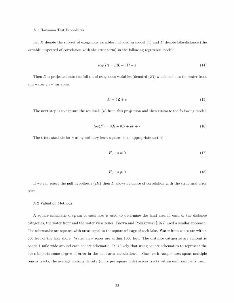
A.1 Hausman Test Procedures

Let X denote the sub-set of exogenous variables included in model (1) and D denote lake-distance (the

variable suspected of correlation with the error term) in the following regression model:

log(P ) = �X+ �D + " (14)

Then D is projected onto the full set of exogenous variables (denoted (Z)) which includes the water front

and water view variables.

D = �Z+ � (15)

The next step is to capture the residuals (�̂) from this projection and then estimate the following model:

log(P ) = �X+ �D + ��̂ + r (16)

The t-test statistic for � using ordinary least squares is an appropriate test of

H0 : � = 0 (17)

H0 : � 6= 0 (18)

If we can reject the null hypothesis (H0) then D shows evidence of correlation with the structural error

term.

A.2 Valuation Methods

A square schematic diagram of each lake is used to determine the land area in each of the distance

categories, the water front and the water view zones. Brown and Pollakowski [1977] used a similar approach.

The schematics are squares with areas equal to the square mileage of each lake. Water front zones are within

500 feet of the lake shore. Water view zones are within 1000 feet. The distance categories are concentric

bands 1 mile wide around each square schematic. It is likely that using square schematics to represent the

lakes imparts some degree of error in the land area calculations. Since each sample area spans multiple

census tracts, the average housing density (units per square mile) across tracts within each sample is used.

22

References

[1] Brookshire, D.S., M.A. Thayer, W.D. Schulze, R.C. d�Arge. March 1982. �Valuing Public Goods: A Comparison

of Survey and Hedonic Approaches.�American Economic Review. 72: 165-177.

[2] Brown, G.M. Jr., H.O. Pollakowski. August 1977. �Economic Value of Shoreline� Review of Economics and

Statistics. 59: 272-278

[3] Cropper, M.L., L.B. Deck, K.E. McConnell, 1988. "On the Choice of Functional Form for Hedonic Price

Functions." The Review of Economics and Statistics, 70(4): 668-675.

[4] Earnhart, D., 2001. �Combining Revealed and Stated Preference Methods to Value Environmental Amenities

at Residential Locations.�Land Economics. 77(1): 12-29.

[5] Freeman, A.M. "The Measurement of Environmental and Resource Values." 2nd Ed. Resources for the Future.

Washington D.C. c2003.

[6] Hardle, W. �Applied Non-Parametric Regression�, Econometric Society Monograph, No. 19, Cambridge

University Press, Cambridge, U.K.,1990

[7] Heien, D.M. 1968. "A Note on Log-Linear Regression." Journal of the American Statistical Association. 63(323):

1034-1038.

[8] Hausman, J.A. 1978. "Speci�cation Tests in Econometrics." Econometrica, 46(6):1251-1271.

[9] Lansford, N.H., L.L. Jones. 1995. "Recreational and Aesthetic Value of Water Using Hedonic Price Analysis."

Journal of Agricultural and Resource Economics. 20(2): 341-355.

[10] Loomis, J., M. Feldman. 2003. "Estimating the Bene�ts of Maintaining Adequate Lake Levels to Homeowners

Using the Hedonic Property Method." Water Resour. Res., 39(9).

[11] Mahan, B.L., S. Polasky, R.M. Adams. 2000. �Valuing Urban Wetlands: A Property Price Approach.� Land

Economics. 76(1): 100-113.

[12] Palmquist, R.B., "Valuing Localized Externalities." Journal of Urban Economics. 31(1):59-68.

[13] Rosen, S. 1974. �Hedonic Prices and Implicit Markets: Product Di¤erentiation in Pure Competition,�Journal

of Political Economy. 82: 34-55.

[14] Stone, M. 1974. �Cross-Validatory Choice and Assessment of Statistical Predictions.� Journal of the Royal

Statistical Society. Series B (methodological). 36 (2): 111-147

23

[15] U.S. Census Bureau. Block Maps. http://ftp2.census.gov/plmap/pl_blk/st18_Indiana/c18105_Monroe/PB18105_000.pdf.

[16] U.S. Census Bureau. Block Maps. http://ftp2.census.gov/plmap/pl_blk/st09_Connecticut/c09001_Fair�eld/PB09001_000.pdf.

[17] U.S. Census Bureau. Block Maps. http://ftp2.census.gov/plmap/pl_blk/st09_Connecticut/c09005_Litch�eld/PB09005_000.pdf.

[18] U.S. Census Bureau. http://www.census.gov/census2000/states/ct.html.

[19] White, H. 1980. �A Heteroskedasticity-Consistent Covariance Matrix Estimator and a Direct Test for

Heteroskedasticity�Econometrica, 48 (4): 817-838.

24