~ 1 ~

Using FEMM to integrate the circuit equations when the slug is fixed in place

I have described in two earlier papers, titled Using FEMM to analyze a coil from a coil gun and

Automating the FEMM-analysis of a coil, Lua scripts which use the FEMM program to construct and

analyze coils from a coil gun. The ideal script would be one which simulates the entire process of firing a

slug from a coil gun. That's the ultimate goal, but I won't get quite that far in this paper. In this paper, I

will use FEMM to simulate the coil gun's circuit when the slug is held in a fixed position.

I will use the same slug and coil that I used in the earlier papers. The coil consists of 78 turns of AWG 16

enameled copper wire wound in two layers around a brass tube which serves as the barrel. The coil is two

inches long. The iron slug is also two inches long and has a diameter of one-half inch. (That is a fairly

big and heavy slug.) The coil is surrounded by an iron housing, whose nominal thickness in all directions

is one-quarter inch.

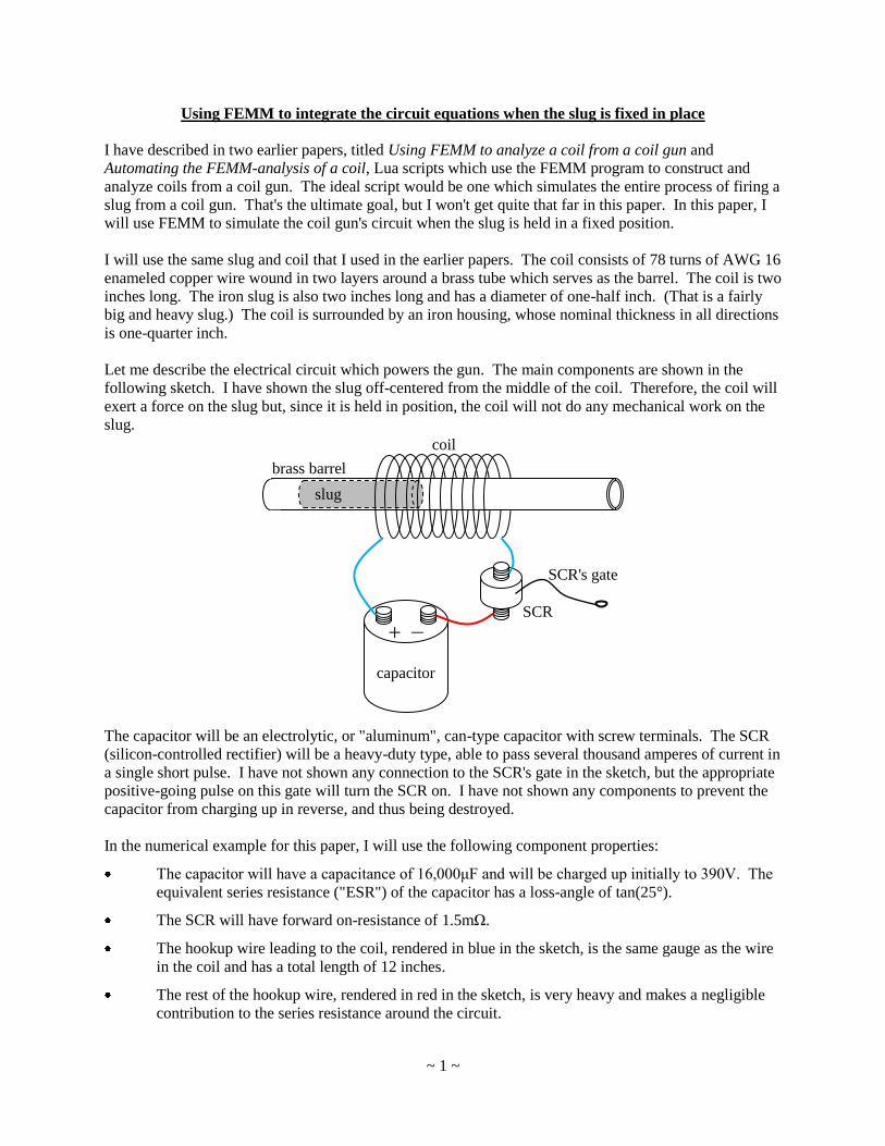
Let me describe the electrical circuit which powers the gun. The main components are shown in the

following sketch. I have shown the slug off-centered from the middle of the coil. Therefore, the coil will

exert a force on the slug but, since it is held in position, the coil will not do any mechanical work on the

slug.

The capacitor will be an electrolytic, or "aluminum", can-type capacitor with screw terminals. The SCR

(silicon-controlled rectifier) will be a heavy-duty type, able to pass several thousand amperes of current in

a single short pulse. I have not shown any connection to the SCR's gate in the sketch, but the appropriate

positive-going pulse on this gate will turn the SCR on. I have not shown any components to prevent the

capacitor from charging up in reverse, and thus being destroyed.

In the numerical example for this paper, I will use the following component properties:

The capacitor will have a capacitance of 16,000μF and will be charged up initially to 390V. The

equivalent series resistance ("ESR") of the capacitor has a loss-angle of tan(25°).

The SCR will have forward on-resistance of 1.5mΩ.

The hookup wire leading to the coil, rendered in blue in the sketch, is the same gauge as the wire

in the coil and has a total length of 12 inches.

The rest of the hookup wire, rendered in red in the sketch, is very heavy and makes a negligible

contribution to the series resistance around the circuit.

coil

brass barrel

SCR

capacitor

SCR's gate

+ –

slug

~ 2 ~

Leakage due to reverse bias is ignored, since I am assuming the gun will be fired within a few

minutes of completing the process of charging the capacitor.

The coil will have the properties we calculated in the earlier papers. We calculated its Ohmic resistance

to be 59.55534mΩ. The total inductance of the coil-and-slug is not constant. In general, the total

inductance will vary, not just with the location of the slug, but with the magnitude of the current as well.

Because the slug is prevented from moving (in this paper), the changes in total inductance will be due

solely to the changes in current.

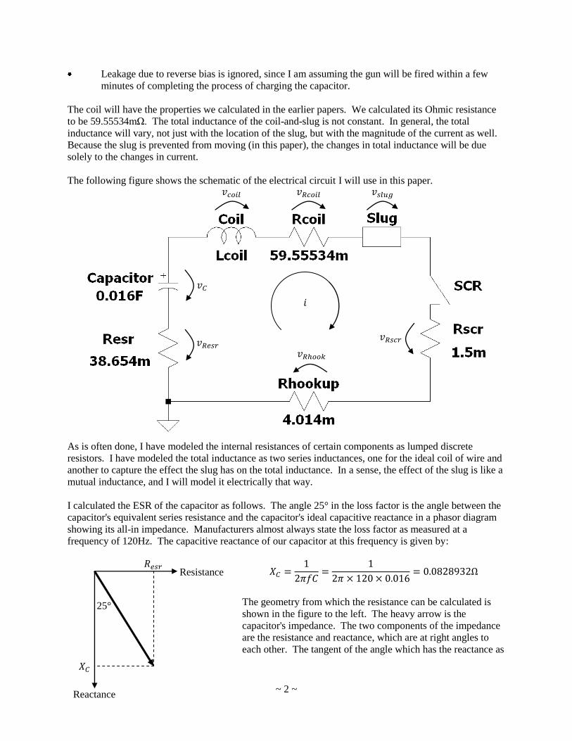
The following figure shows the schematic of the electrical circuit I will use in this paper.

As is often done, I have modeled the internal resistances of certain components as lumped discrete

resistors. I have modeled the total inductance as two series inductances, one for the ideal coil of wire and

another to capture the effect the slug has on the total inductance. In a sense, the effect of the slug is like a

mutual inductance, and I will model it electrically that way.

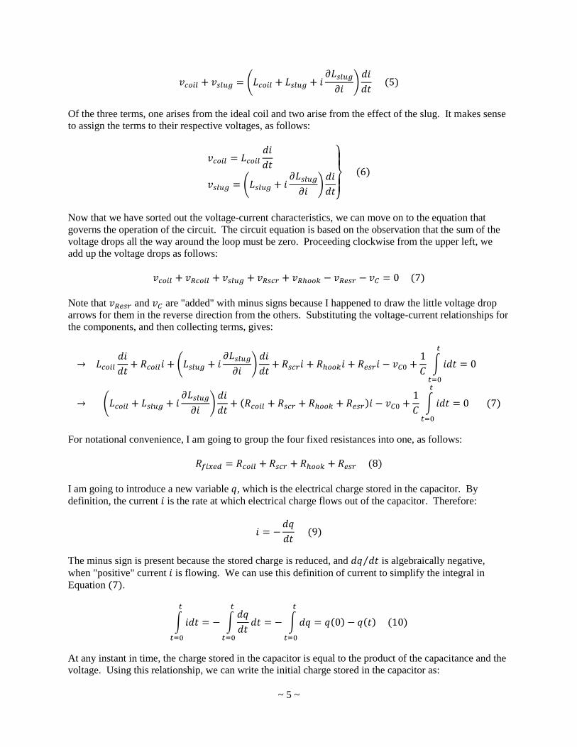
I calculated the ESR of the capacitor as follows. The angle 25° in the loss factor is the angle between the

capacitor's equivalent series resistance and the capacitor's ideal capacitive reactance in a phasor diagram

showing its all-in impedance. Manufacturers almost always state the loss factor as measured at a

frequency of 120Hz. The capacitive reactance of our capacitor at this frequency is given by:

The geometry from which the resistance can be calculated is

shown in the figure to the left. The heavy arrow is the

capacitor's impedance. The two components of the impedance

are the resistance and reactance, which are at right angles to

each other. The tangent of the angle which has the reactance as

Resistance

Reactance

25°

~ 3 ~

its "near" side and the resistance as its "far" side is 25°. Using trigonometry, we can say that:

I calculated the resistance of the hookup wire as follows. The default conductivity for copper wire in the

FEMM database is 58 MS/m. These units are mega-Siemens per meter, so this conductivity can also be

written as 58 106 S/m. Since conductivity is the reciprocal of resistivity, the resistivity can be written as

1.724 10-8

Ωm. This resistivity is the resistance of a cube of this material (copper) which has one-meter

sides. It is implicit in the definition that the cube's cross-sectional area, perpendicular to the flow of

current, is one square meter. In one of the earlier papers, I stated that the diameter of AWG #16 wire is

1.291183 millimeters. The corresponding cross-sectional area of this wire is

mm2, or m

2. I am going to ignore the correction which would take into

account the enamel coating on the wire, and simply divide the resistivity by the cross-sectional area of the

wire to get the resistance of a one-meter length, as follows: , or

. The 12 inches of hookup wire will have a resistance of

, or 4.014 mΩ.

(Some purists may object to the number of significant digits to which I have expressed these quantities.

Quite right. There is no possibility that the circuit is going to have exactly these values. Perhaps they

will not even be within 50%. I am simply trying to avoid the uncertainty which arises when figures

shown in one part of the text are repeated elsewhere, or in the code, with a different number of digits.)

I have shown the SCR as a simple on-off switch. The switch will close at start time in the

simulation, at which time the internal resistance of the SCR (1.5mΩ) will come to bear.

The circuit equations in continuous-time form

In order to simulate the circuit, we need to discretize the circuit equations. The place to start is to write

down the circuit equations in their usual continuous-time form. There is only one current , whose

assumed direction when algebraically positive is shown by the circular arrow in the schematic. Symbols

with small letters indicate instantaneous values. I have also defined seven instantaneous voltages:

The voltage drop over the ideal capacitor is .

The voltage drop over the equivalent series resistance of the real capacitor is .

The voltage drop over the ideal coil is .

The voltage drop over the real coil's Ohmic resistance is .

The voltage drop due to the effect of the slug is .

The voltage drop over the SCR when it is conducting is .

The voltage drop over the hookup wire is .

All of these voltages drops will be assumed to be algebraically positive when the voltage decreases in the

direction shown by the small arrows overlaid on the schematic.

The standard voltage-as-a-function-of-current relationships for the components in this circuit are the

following:

~ 4 ~

The symbol is the starting voltage on the capacitor. The voltage drop over the ideal capacitor

starts at at time in the simulation, and will decrease from that starting voltage as current flows

out of the capacitor. The voltage drops over the four resistances are given by Ohm's Law. The only

voltage drop that is unusual is the one for the combination of the ideal coil and the slug.

I have used the symbol for the total inductance of the combination of the ideal coil and the slug.

The product of this total inductance and the current is the flux which connects the individual turns in the

coil with each other and with the slug. The total voltage drop over the combination is the

rate-of-change of the flux, which is represented in the Calculus as the time derivative of the flux. I will

represent the total inductance as the sum of an inductance for the ideal coil and a second inductance for

the effect of the slug, as follows:

I will treat the inductance of the ideal coil as being constant, fixed at its value when no current, or

only an extremely small amount of current, flows through the ideal coil. All of the changes which arise

from subsequent changes in the current will be attributed to the presence of the slug, and included in

. Noting that is constant, we can expand the time derivative as follows:

It is true that will change with time as the current rises and falls. But, it is not the passage of time

per se that causes the change in the slug's effective inductance, it is the change in the current. is

really a function of current , rather than time . For this reason, we can express the rate-of-change of

with respect to time in terms of its rate-of-change with respect to current. This is done using a

partial derivative, as follows.

I will explain below how we calculate the rate-of-change of with respect to current. In the

meantime, we can substitute Equation into Equation to get:

~ 5 ~

Of the three terms, one arises from the ideal coil and two arise from the effect of the slug. It makes sense

to assign the terms to their respective voltages, as follows:

Now that we have sorted out the voltage-current characteristics, we can move on to the equation that

governs the operation of the circuit. The circuit equation is based on the observation that the sum of the

voltage drops all the way around the loop must be zero. Proceeding clockwise from the upper left, we

add up the voltage drops as follows:

Note that and are "added" with minus signs because I happened to draw the little voltage drop

arrows for them in the reverse direction from the others. Substituting the voltage-current relationships for

the components, and then collecting terms, gives:

For notational convenience, I am going to group the four fixed resistances into one, as follows:

I am going to introduce a new variable , which is the electrical charge stored in the capacitor. By

definition, the current is the rate at which electrical charge flows out of the capacitor. Therefore:

The minus sign is present because the stored charge is reduced, and is algebraically negative,

when "positive" current is flowing. We can use this definition of current to simplify the integral in

Equation .

At any instant in time, the charge stored in the capacitor is equal to the product of the capacitance and the

voltage. Using this relationship, we can write the initial charge stored in the capacitor as:

~ 6 ~

Substituting Equations , and into the circuit equation gives:

This is the differential equation we are going to integrate numerically. If there was a closed-form

solution, so that we could use the Calculus, the implicit assumption would be that the differentials in time

become vanishingly small. Integrating numerically using a computer code requires that the steps in

time, say , be small but still finite.

We will start off the numerical integration using the same two initial conditions we would use to calculate

the constants of integration in a closed-form solution. The initial charge stored in the capacitor is related

to the initial voltage drop over the capacitor by . Secondly, at the outset, there is no

current flowing, so .

Summary of the numerical integration procedure

For the purpose of the following explanation, assume that we have just completed the st time step in

the numerical integration. We will have updated all of the circuit variables to the end of this time step. In

the continuum of time, the end of the st time step is coincident with the start of the

th time step. For

consistent notion, I will use the following symbols, all of which are assumed to be known at the start of

the th time step.

is the charge stored in the capacitor at the start of the th time step and

is the current at the start of the th time step.

Here is how we will proceed.

Step #1 - First FEMM analysis

We will run a FEMM analysis. I will use the same geometry for this problem that I used in the two

earlier papers. The Lua script constructs the geometry with the leading edge of the slug three-quarters of

an inch shy of the center of the coil. I am going to leave the slug fixed in this location for the entire

simulation. The only other input we need to specify before a FEMM analysis is the instantaneous current,

which we happen to know. It is . The FEMM analysis will give us two things: (i) the total

inductance of the coil and (ii) the force exerted on the slug. The analysis in this paper does not refer to

the force. All we need from the FEMM analysis is the total inductance . We can calculate the

part of this total inductance which is attributable to the slug by subtracting the inductance of the ideal coil

alone, which we will have calculated in a separate FEMM analysis done before starting the integration.

Step #2 - Second FEMM analysis

We will run a second FEMM analysis. The purpose of this analysis is to calculate the rate at which

changes as the current changes. I am going to use brute force to estimate the partial derivative. (There

~ 7 ~

are ways to use the results from previous time steps in the numerical procedure to estimate this derivative,

but I am not going to use them.) I am going to re-run the FEMM analysis with a current which is 100

Amperes larger than . This will give us a revised total inductance, for which I will use the symbol

. The slug's inductance which corresponds to this revised total inductance is:

The partial derivative is defined as the change in due to an infinitesimally small change

in current, when nothing else changes. The qualifier is important; nothing else is changed in Step #2

other than the current. The change in current I am using – 100 Amperes – is certainly not infinitesimally

small, but does give us the approximation:

Step #3 - Calculate the time-rate-of-change of the current using the differential equation

We will evaluate the right-hand side of Equation using the values of all the variables at the start of

this th time step. The differential equation must apply at every instant in time, including this particular

instant. The calculation is:

Step #4 - Assume the time-rate-of-change of the current is constant

We will assume that the duration of the time step is so short that the derivative calculated in Step #3

can be treated as if it remained constant throughout the whole time step. In the Lua script, I have made

the time steps 10μs long. The easiest way to check if the duration of the time steps is "short enough" is to

re-run the simulation using a slightly longer or slightly shorter time step. If the results of the simulation

do not change materially, then the time step is satisfactory.

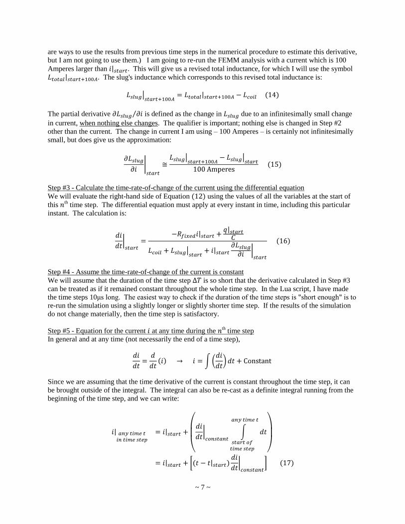
Step #5 - Equation for the current at any time during the th time step

In general and at any time (not necessarily the end of a time step),

Since we are assuming that the time derivative of the current is constant throughout the time step, it can

be brought outside of the integral. The integral can also be re-cast as a definite integral running from the

beginning of the time step, and we can write:

~ 8 ~

Step #6 - Equation for the charge at any time during the th time step

In general and at any time (not necessarily the end of a time step),

In Step #5, we derived an expression for as a function of time. We can explicitly integrate a second time

to find the stored charge at any time during this time step. We get:

It should be understood that Equations and are functions of time and can be used at any time

during this time step, not just at the end of the time step.

Step #7 - Evaluate the current and the charge at the end of the time step

We do have a particular interest in knowing the values of and at the end of this time step, since they

will be two of the "input" values we will need when we start the next time step. Since the time step is

long, then the elapsed time will be equal to at the end of the time step, and we can write:

Step #8 - Calculate the voltage drop over the capacitor at the end of the time step

Although I did not say so above, we will also have calculated the voltage drop over the ideal capacitor at

the end of the st time step. Now that we are at the end of the

th time step, it is timely to update that

calculation. We can do this directly, as follows:

Step #9 - Calculate the voltage drops over the resistances at the end of the time step

The last step is to calculate the voltage drops over the various resistances in the circuit. It is enough for

our purposes to compute these voltages at the end of the time step.

~ 9 ~

Does the SCR need to be turned off?

At all times during the simulation, we need to keep our eye on the direction of the current . Like a

standard diode, the SCR allows current to flow in one direction but not the other. In fact, the SCR will

turn itself off if the current flowing through its main channel falls below a certain level, called the

threshold current. In a subsequent paper, I will look at a subcircuit whose purpose is to turn the SCR on

at the start of a run. The SCR I intend to use in look at in that subcircuit has a holding current of about

600mA. This is a small current compared to the thousands of Amperes which will flow when the main

circuit is really providing power to accelerate the slug.

There should not be any phenomena involving voltage spikes when the SCR turns itself off due to low

current flow. Sudden cessation of the current flowing through a coil will cause it to suddenly release all

of its magnetic energy. This can lead to very high voltage spikes, which can be high enough to destroy

components in the circuit. However, the strength of the coil's magnetic field is proportional to the

current. When the current is small, the strength of the magnetic field is also small. Fortunately for us, it

is in just these circumstances that the SCR will turn itself off.

Other features of the Lua script

The Lua script saves results to a text file named "Coil_Gun_Simulation.txt" which it will create in the same

directory as the shortcut which was used to invoke the FEMM program. Results are not saved at the end

of every time step, but at intervals specified by the user. The variable SaveInterval is an integer which the

user sets to the number of time steps between save events. The script uses another integer named

SaveCounter which is incremented every time step and determines by overflow when it is time to save

results.

The Lua script formats the results is writes to the output file. This aligns all the figures into columns

which can easily be imported into Excel. I should point out that there are too many columns to fit on a

standard-sized page (8½" by 11") in portrait format. In order to prevent Excel from mixing up columns

during the import, the page format must be changed. This is not hard. Open the output file using

NotePad or some other text editor, and change the page setup so that it is legal-sized (8½" by 14") and has

landscape orientation. That gives ample width for all columns to have their own space on the page.

The Lua script prints a minimum amount of information to the screen during the simulation. It only prints

the simulation time, the current, the slug's inductance and rate-of-change-with-current of the slug's

inductance. That is enough for the user to gauge the rate at which progress is being made.

The Lua script ends the simulation when the current falls below one Ampere.

Results from the first run

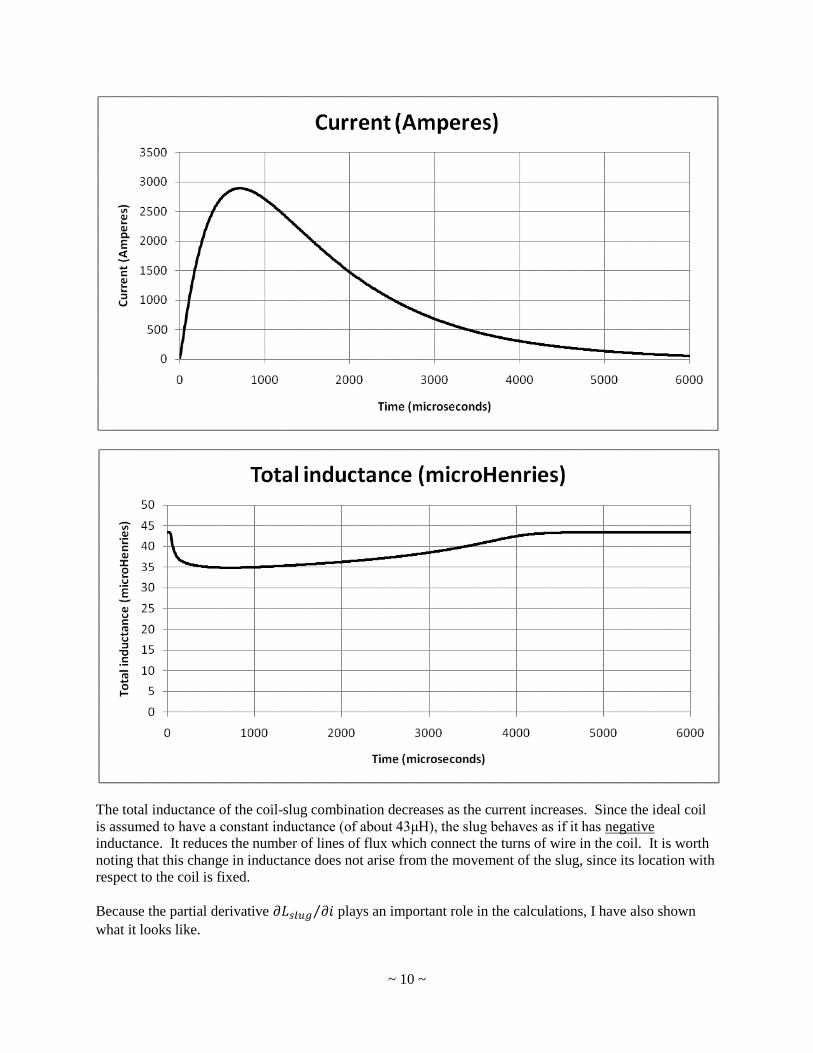
The following two graphs show the waveforms of the current and the total inductance with time. The

current goes up, reaching a peak just under 3,000 Amperes at about 800μs, and then it goes down. The

circuit being used here is an L-R-C circuit. Generally speaking, L-R-C circuits shows two types of

behaviour. Depending on the ratios among the inductance, resistance and capacitance, the waveforms can

be either: (i) a fast exponential rise followed by a slower exponential decay, or (ii) the same rise and fall

overlaid with a sinusoidal oscillation. It seems that the ratios among the components I chose for this

circuit lead to the former type of response.

~ 10 ~

The total inductance of the coil-slug combination decreases as the current increases. Since the ideal coil

is assumed to have a constant inductance (of about 43μH), the slug behaves as if it has negative

inductance. It reduces the number of lines of flux which connect the turns of wire in the coil. It is worth

noting that this change in inductance does not arise from the movement of the slug, since its location with

respect to the coil is fixed.

Because the partial derivative plays an important role in the calculations, I have also shown

what it looks like.

~ 11 ~

The spike which occurs about 40μs into the run is not too big a concern. The time step in this run was

10μs long, and the numerical procedure needs a couple of time steps to get itself established. It is during

these early microseconds that the slug passes through saturation, when the nature of the dependence of the

inductance on the current changes significantly.

Conservation of energy

I want to confirm that energy is conserved during the process. If the mathematical model is flawed, a test

of energy conservation will likely fail. Undertaking this analysis serves a practical purpose as well. It

will help us set bounds on our choice of simulation parameters. For example, it will help us determine

how long the time steps can be allowed to be.

At the instant before the coil gun is fired, there is only one source of energy. That is the electrostatic

energy stored inside the capacitor. As soon as we "close the switch" by turning on the SCR, the energy

stored inside the capacitor will start to be converted into two other types:

magnetic energy stored inside the magnetic field generated in and around the coil and slug and

heat energy burned off by the fixed resistors.

I am going to keep track of the energy balance by calculating the change in each type of energy during

every time step. At any time during the simulation, the cumulative sum of the changes since the start of

the simulation should be zero. As a practical matter, one could choose to do the test at the start of each

time step, or the end of each time step or, perhaps, even at both times. I have chosen to reconcile the

energy balance at the end of every time step.

Some of the energy calculations can be improved by understanding the waveform of the current which the

numerical procedure produces. The principal differential equation has the form:

~ 12 ~

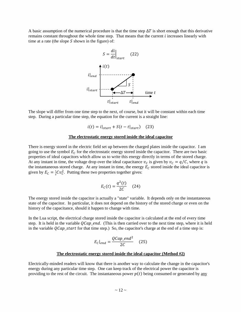
A basic assumption of the numerical procedure is that the time step is short enough that this derivative

remains constant throughout the whole time step. That means that the current increases linearly with

time at a rate (the slope shown in the figure) of:

The slope will differ from one time step to the next, of course, but it will be constant within each time

step. During a particular time step, the equation for the current is a straight line:

The electrostatic energy stored inside the ideal capacitor

There is energy stored in the electric field set up between the charged plates inside the capacitor. I am

going to use the symbol for the electrostatic energy stored inside the capacitor. There are two basic

properties of ideal capacitors which allow us to write this energy directly in terms of the stored charge.

At any instant in time, the voltage drop over the ideal capacitance is given by , where is

the instantaneous stored charge. At any instant in time, the energy stored inside the ideal capacitor is

given by . Putting these two properties together gives:

The energy stored inside the capacitor is actually a "state" variable. It depends only on the instantaneous

state of the capacitor. In particular, it does not depend on the history of the stored charge or even on the

history of the capacitance, should it happen to change with time.

In the Lua script, the electrical charge stored inside the capacitor is calculated at the end of every time

step. It is held in the variable . (This is then carried over to the next time step, where it is held

in the variable for that time step.) So, the capacitor's charge at the end of a time step is:

The electrostatic energy stored inside the ideal capacitor (Method #2)

Electrically-minded readers will know that there is another way to calculate the change in the capacitor's

energy during any particular time step. One can keep track of the electrical power the capacitor is

providing to the rest of the circuit. The instantaneous power being consumed or generated by any

time

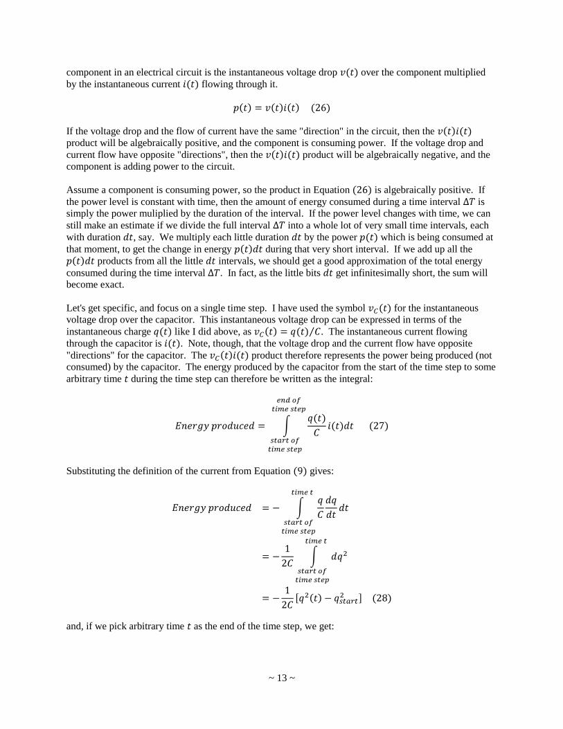
~ 13 ~

component in an electrical circuit is the instantaneous voltage drop over the component multiplied

by the instantaneous current flowing through it.

If the voltage drop and the flow of current have the same "direction" in the circuit, then the

product will be algebraically positive, and the component is consuming power. If the voltage drop and

current flow have opposite "directions", then the product will be algebraically negative, and the

component is adding power to the circuit.

Assume a component is consuming power, so the product in Equation is algebraically positive. If

the power level is constant with time, then the amount of energy consumed during a time interval is

simply the power muliplied by the duration of the interval. If the power level changes with time, we can

still make an estimate if we divide the full interval into a whole lot of very small time intervals, each

with duration , say. We multiply each little duration by the power which is being consumed at

that moment, to get the change in energy during that very short interval. If we add up all the

products from all the little intervals, we should get a good approximation of the total energy

consumed during the time interval . In fact, as the little bits get infinitesimally short, the sum will

become exact.

Let's get specific, and focus on a single time step. I have used the symbol for the instantaneous

voltage drop over the capacitor. This instantaneous voltage drop can be expressed in terms of the

instantaneous charge like I did above, as . The instantaneous current flowing

through the capacitor is . Note, though, that the voltage drop and the current flow have opposite

"directions" for the capacitor. The product therefore represents the power being produced (not

consumed) by the capacitor. The energy produced by the capacitor from the start of the time step to some

arbitrary time during the time step can therefore be written as the integral:

Substituting the definition of the current from Equation gives:

and, if we pick arbitrary time as the end of the time step, we get:

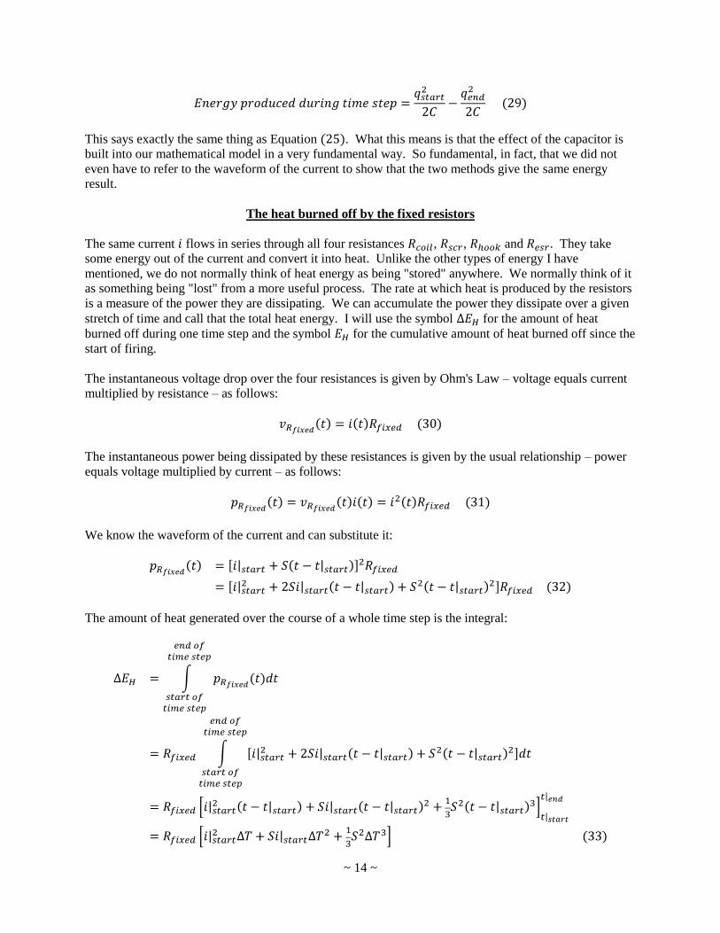
~ 14 ~

This says exactly the same thing as Equation . What this means is that the effect of the capacitor is

built into our mathematical model in a very fundamental way. So fundamental, in fact, that we did not

even have to refer to the waveform of the current to show that the two methods give the same energy

result.

The heat burned off by the fixed resistors

The same current flows in series through all four resistances , , and . They take

some energy out of the current and convert it into heat. Unlike the other types of energy I have

mentioned, we do not normally think of heat energy as being "stored" anywhere. We normally think of it

as something being "lost" from a more useful process. The rate at which heat is produced by the resistors

is a measure of the power they are dissipating. We can accumulate the power they dissipate over a given

stretch of time and call that the total heat energy. I will use the symbol for the amount of heat

burned off during one time step and the symbol for the cumulative amount of heat burned off since the

start of firing.

The instantaneous voltage drop over the four resistances is given by Ohm's Law – voltage equals current

multiplied by resistance – as follows:

The instantaneous power being dissipated by these resistances is given by the usual relationship – power

equals voltage multiplied by current – as follows:

We know the waveform of the current and can substitute it:

The amount of heat generated over the course of a whole time step is the integral:

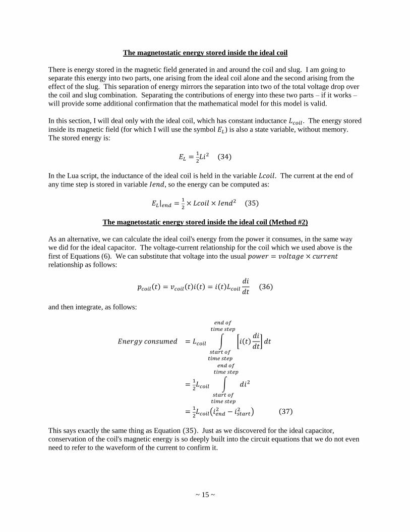
~ 15 ~

The magnetostatic energy stored inside the ideal coil

There is energy stored in the magnetic field generated in and around the coil and slug. I am going to

separate this energy into two parts, one arising from the ideal coil alone and the second arising from the

effect of the slug. This separation of energy mirrors the separation into two of the total voltage drop over

the coil and slug combination. Separating the contributions of energy into these two parts – if it works –

will provide some additional confirmation that the mathematical model for this model is valid.

In this section, I will deal only with the ideal coil, which has constant inductance . The energy stored

inside its magnetic field (for which I will use the symbol ) is also a state variable, without memory.

The stored energy is:

In the Lua script, the inductance of the ideal coil is held in the variable . The current at the end of

any time step is stored in variable , so the energy can be computed as:

The magnetostatic energy stored inside the ideal coil (Method #2)

As an alternative, we can calculate the ideal coil's energy from the power it consumes, in the same way

we did for the ideal capacitor. The voltage-current relationship for the coil which we used above is the

first of Equations (6). We can substitute that voltage into the usual

relationship as follows:

and then integrate, as follows:

This says exactly the same thing as Equation . Just as we discovered for the ideal capacitor,

conservation of the coil's magnetic energy is so deeply built into the circuit equations that we do not even

need to refer to the waveform of the current to confirm it.

~ 16 ~

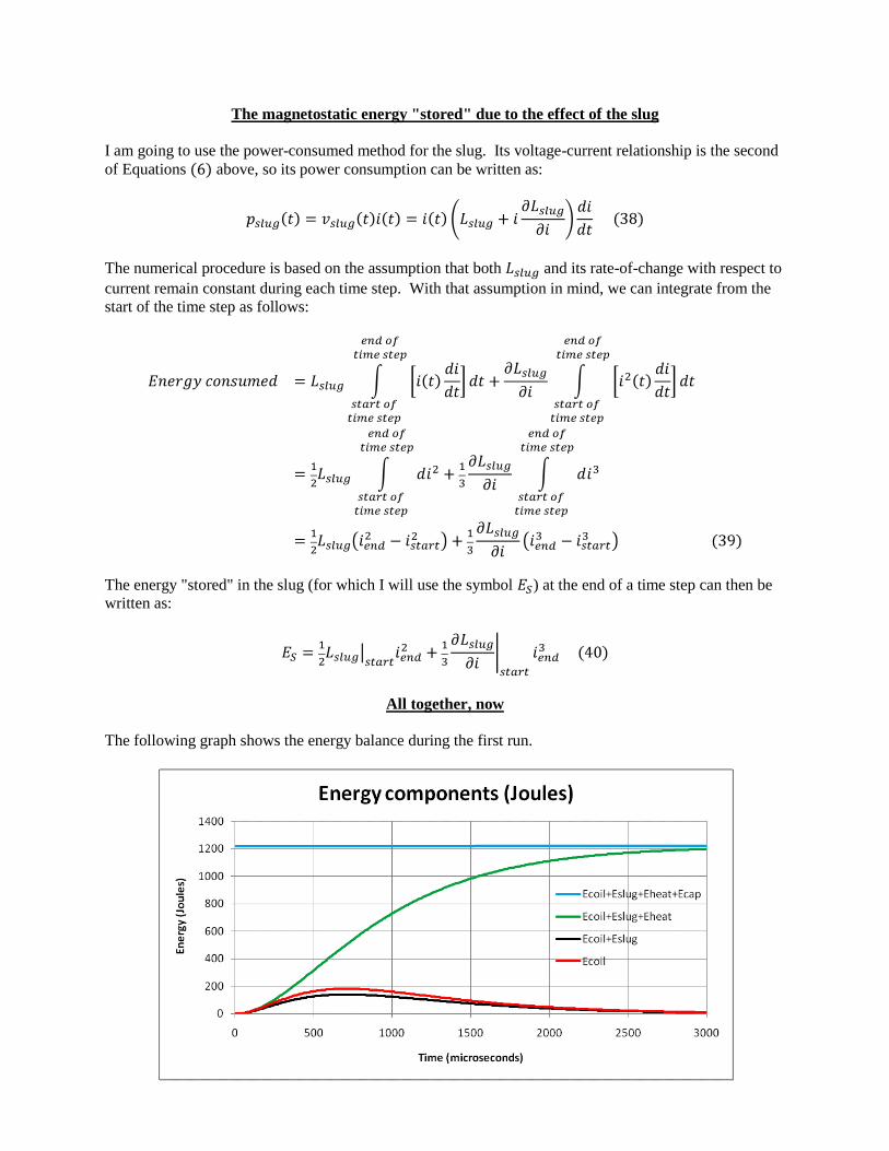
The magnetostatic energy "stored" due to the effect of the slug

I am going to use the power-consumed method for the slug. Its voltage-current relationship is the second

of Equations above, so its power consumption can be written as:

The numerical procedure is based on the assumption that both and its rate-of-change with respect to

current remain constant during each time step. With that assumption in mind, we can integrate from the

start of the time step as follows:

The energy "stored" in the slug (for which I will use the symbol ) at the end of a time step can then be

written as:

All together, now

The following graph shows the energy balance during the first run.

~ 17 ~

In this graph, I have shown the four components of the total energy added on top of each other. The red

curve is simply the energy stored in the ideal coil at any given time during the simulation. The black

curve is the sum of the energy stored in the coil and the energy "stored" in the slug. Note that this total is

actually less than the coil's energy alone. Because it acts like a negative inductance, the slug actually

decreases the total energy stored in the coil-slug combination. The green curve shows the energy stored

in the coil-slug combination plus the heat burned off by the four fixed resistances since the start of the

run. Lastly, the blue curve shows the energy stored in the capacitor added to the other energy

components. At the start of the run, the capacitor held 1216.8 Joules of energy. When all is said and

done, all of that has been converted into heat.

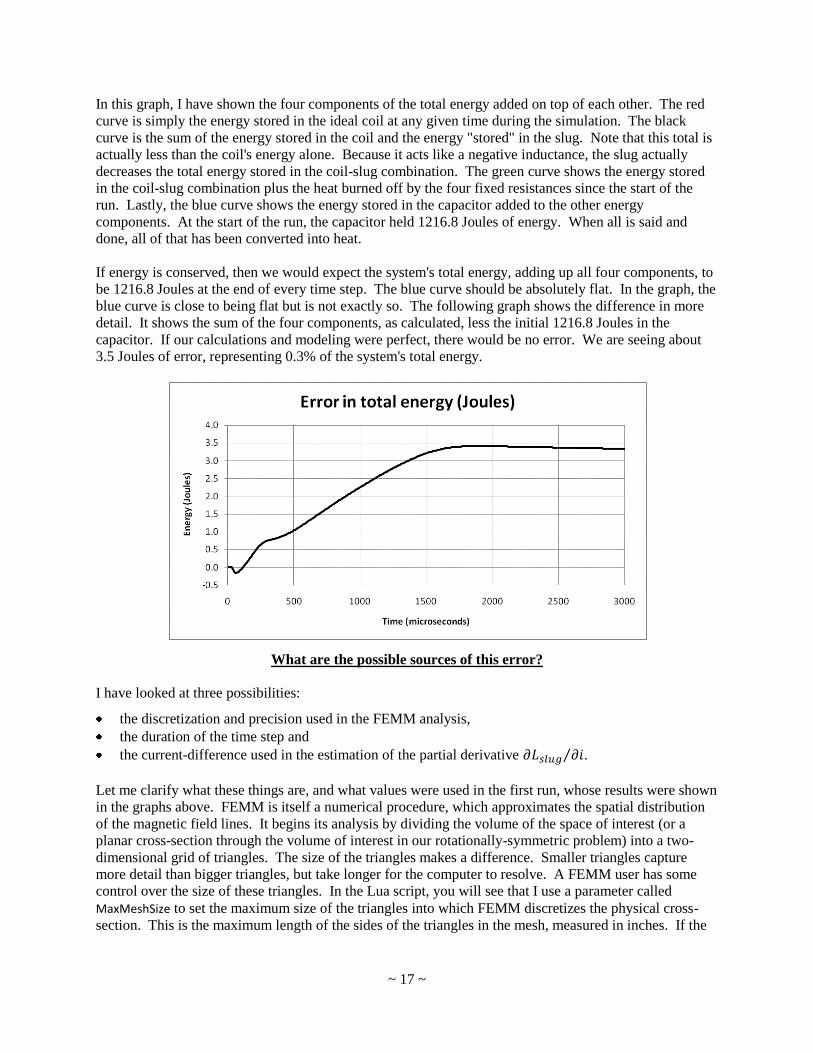
If energy is conserved, then we would expect the system's total energy, adding up all four components, to

be 1216.8 Joules at the end of every time step. The blue curve should be absolutely flat. In the graph, the

blue curve is close to being flat but is not exactly so. The following graph shows the difference in more

detail. It shows the sum of the four components, as calculated, less the initial 1216.8 Joules in the

capacitor. If our calculations and modeling were perfect, there would be no error. We are seeing about

3.5 Joules of error, representing 0.3% of the system's total energy.

What are the possible sources of this error?

I have looked at three possibilities:

the discretization and precision used in the FEMM analysis,

the duration of the time step and

the current-difference used in the estimation of the partial derivative .

Let me clarify what these things are, and what values were used in the first run, whose results were shown

in the graphs above. FEMM is itself a numerical procedure, which approximates the spatial distribution

of the magnetic field lines. It begins its analysis by dividing the volume of the space of interest (or a

planar cross-section through the volume of interest in our rotationally-symmetric problem) into a two-

dimensional grid of triangles. The size of the triangles makes a difference. Smaller triangles capture

more detail than bigger triangles, but take longer for the computer to resolve. A FEMM user has some

control over the size of these triangles. In the Lua script, you will see that I use a parameter called

MaxMeshSize to set the maximum size of the triangles into which FEMM discretizes the physical cross-

section. This is the maximum length of the sides of the triangles in the mesh, measured in inches. If the

~ 18 ~

user does not specify a maximum triangle size, then FEMM makes its own assessment of an appropriate

size. In the first run, I set MaxMeshSize to 0.01 inches, which is FEMM's default value.

FEMM uses a second parameter as well, which determines the precision to which the FEMM analysis is

carried out. The FEMM analysis is iterative. The sets of equations which FEMM uses cannot be solved

in a single pass. FEMM has to repeat its calculations over and over, revising the variables in the proposed

solution at the start of each iteration based on the errors encountered during the previous iteration. A

FEMM user has some control over the desired precision. The default precision used by FEMM is 10-8

. In

the first run, I set the precision to this default value.

The numerical integration process assumes that certain variables remain constant during the whole of

each time step, although they do change from one time step to the next. The longer the time steps are, the

more time such linearized variables have to depart from reality. Shorter time steps reduce the

linearization error, but take longer for the computer to work through.

I used a "brute force" method to estimate the partial derivative at the start of each time step.

Step #1 of the procedure is a FEMM analysis to calculate the value of at the current .

Compter experts would be horrified that I would do a second FEMM analysis to calculate a different

inductance using a different current. In the first run, I chose to make the different current 100 Amperes

greater than the starting current. Why not 10 Amperes greater? Or just one Ampere greater? Good

questions. I chose a relatively large change in current in order to ensure that the partial derivative was not

swamped by noise from the FEMM analysis. Noise can arise because the derivative relies on taking the

difference between two FEMM analyses. The closer the two currents are, the less reliable the differences

between the calculated inductances become. This is magnified by the difference between the currents in

the denominator. The closer the two currents are, the more the difference between the inductances is

scaled up. The way to find a happy medium is to see what happens using a different current difference.

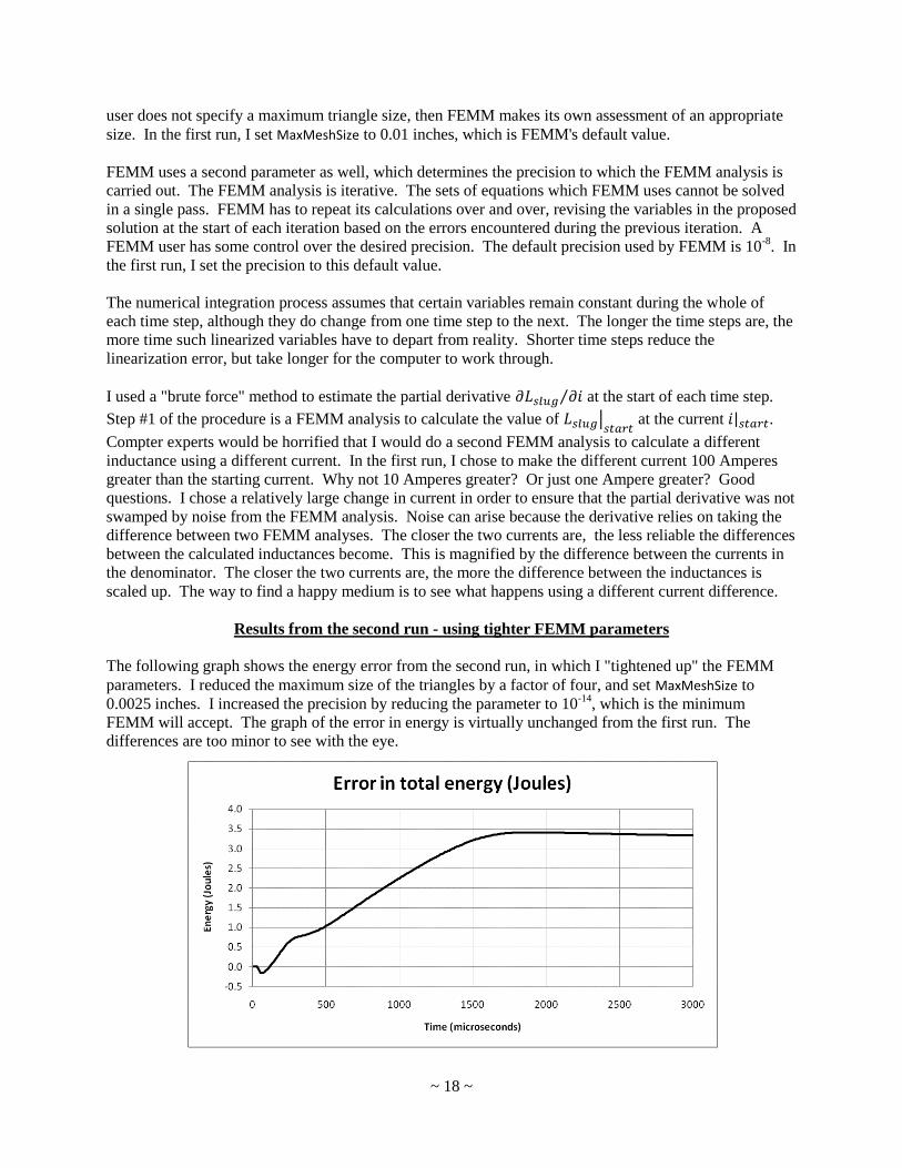
Results from the second run - using tighter FEMM parameters

The following graph shows the energy error from the second run, in which I "tightened up" the FEMM

parameters. I reduced the maximum size of the triangles by a factor of four, and set MaxMeshSize to

0.0025 inches. I increased the precision by reducing the parameter to 10-14

, which is the minimum

FEMM will accept. The graph of the error in energy is virtually unchanged from the first run. The

differences are too minor to see with the eye.

~ 19 ~

Results from the third run - using a shorter time step

The following graph shows the energy error from the third run, in which I reduced the time step by a

factor of ten, to 1μs. Just to be clear, this run used the same FEMM parameters as the first run: 0.01 inch

triangles and 10-8

precision. Shorter time steps make a considerable difference. The maximum energy

error is about 1.2 Joules, or 0.1% of the system error, and the residual error at the end of the run is only

0.2 Joules.

Results from the fourth run - using a smaller current-difference

In the fourth run, I reduced the current-difference for estimating by a factor of ten, to 10

Amperes. I kept the time step at 1μs, as in the third run, and used the same FEMM parameters as the first

run: 0.01 inch triangles and 10-8

precision.

~ 20 ~

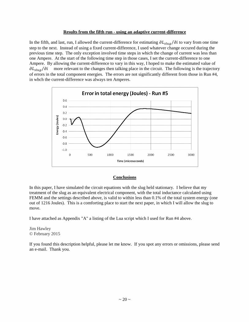
Results from the fifth run - using an adaptive current-difference

In the fifth, and last, run, I allowed the current-difference for estimating to vary from one time

step to the next. Instead of using a fixed current-difference, I used whatever change occured during the

previous time step. The only exception involved time steps in which the change of current was less than

one Ampere. At the start of the following time step in those cases, I set the current-difference to one

Ampere. By allowing the current-difference to vary in this way, I hoped to make the estimated value of

more relevant to the changes then talking place in the circuit. The following is the trajectory

of errors in the total component energies. The errors are not significantly different from those in Run #4,

in whch the current-difference was always ten Amperes.

Conclusions

In this paper, I have simulated the circuit equations with the slug held stationary. I believe that my

treatment of the slug as an equivalent electrical component, with the total inductance calculated using

FEMM and the settings described above, is valid to within less than 0.1% of the total system energy (one

out of 1216 Joules). This is a comforting place to start the next paper, in which I will allow the slug to

move.

I have attached as Appendix "A" a listing of the Lua script which I used for Run #4 above.

Jim Hawley

© February 2015

If you found this description helpful, please let me know. If you spot any errors or omissions, please send

an e-mail. Thank you.

~ 21 ~

Appendix "A"

Listing of the Lua script for Run #4

-- Definition of FEMM solver parameters MaxMeshSize = 0.01 MaxResidual = 1E-8 -- Definition of Groups -- Group(0) is the air -- Group(1) is the coil -- Group(2) is the projectile, or slug -- Group(3) is the far gate annulus -- Group(4) is the near gate annulus -- Group(5) is the surrounding sheath -- Definition of slug parameters, in inches SlugLength=2 SlugRadius=0.5/2 SlugMaterial='Pure Iron' SlugLeadingEdgeZ=-0.75 -- Definition of coil parameters, in inches CoilLength=2 CoilInnerRadius=0.625/2 WireGauge=16 NumLayers=2 -- Definition of current flowing through the coil CoilCurrent=1000 -- Thickness of phenolic annuli, in inches PhenolicThickness=1/32 -- Definition of far gate, in inches -- (Set IncludeFarGate=0 to eliminate the far gate entirely.) IncludeFarGate=1 FarGateThickness=1/4 FarGateStandoff=PhenolicThickness FarGateMaterial='Pure Iron' -- Definition of near gate, in inches -- (Set IncludeNearGate=0 to eliminate the far gate entirely.) IncludeNearGate=1 NearGateThickness=1/4 NearGateStandoff=PhenolicThickness NearGateMaterial='Pure Iron'

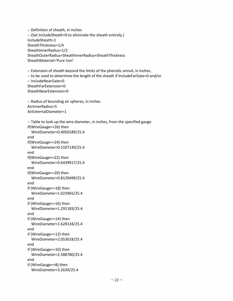
~ 22 ~

-- Definition of sheath, in inches -- (Set IncludeSheath=0 to eliminate the sheath entirely.) IncludeSheath=1 SheathThickness=1/4 SheathInnerRadius=1/2 SheathOuterRadius=SheathInnerRadius+SheathThickness SheathMaterial='Pure Iron' -- Extension of sheath beyond the limits of the phenolic annuli, in inches, -- to be used to determine the length of the sheath if IncludeFarGate=0 and/or -- IncludeNearGate=0. SheathFarExtension=0 SheathNearExtension=0 -- Radius of bounding air spheres, in inches AirInnerRadius=5 AirExternalDiameter=1 -- Table to look up the wire diameter, in inches, from the specified gauge if(WireGauge==26) then WireDiameter=0.4050189/25.4 end if(WireGauge==24) then WireDiameter=0.5107140/25.4 end if(WireGauge==22) then WireDiameter=0.6439917/25.4 end if(WireGauge==20) then WireDiameter=0.8120499/25.4 end if (WireGauge==18) then WireDiameter=1.023965/25.4 end if (WireGauge==16) then WireDiameter=1.291183/25.4 end if (WireGauge==14) then WireDiameter=1.628134/25.4 end if (WireGauge==12) then WireDiameter=2.053018/25.4 end if (WireGauge==10) then WireDiameter=2.588780/25.4 end if (WireGauge==8) then WireDiameter=3.2639/25.4

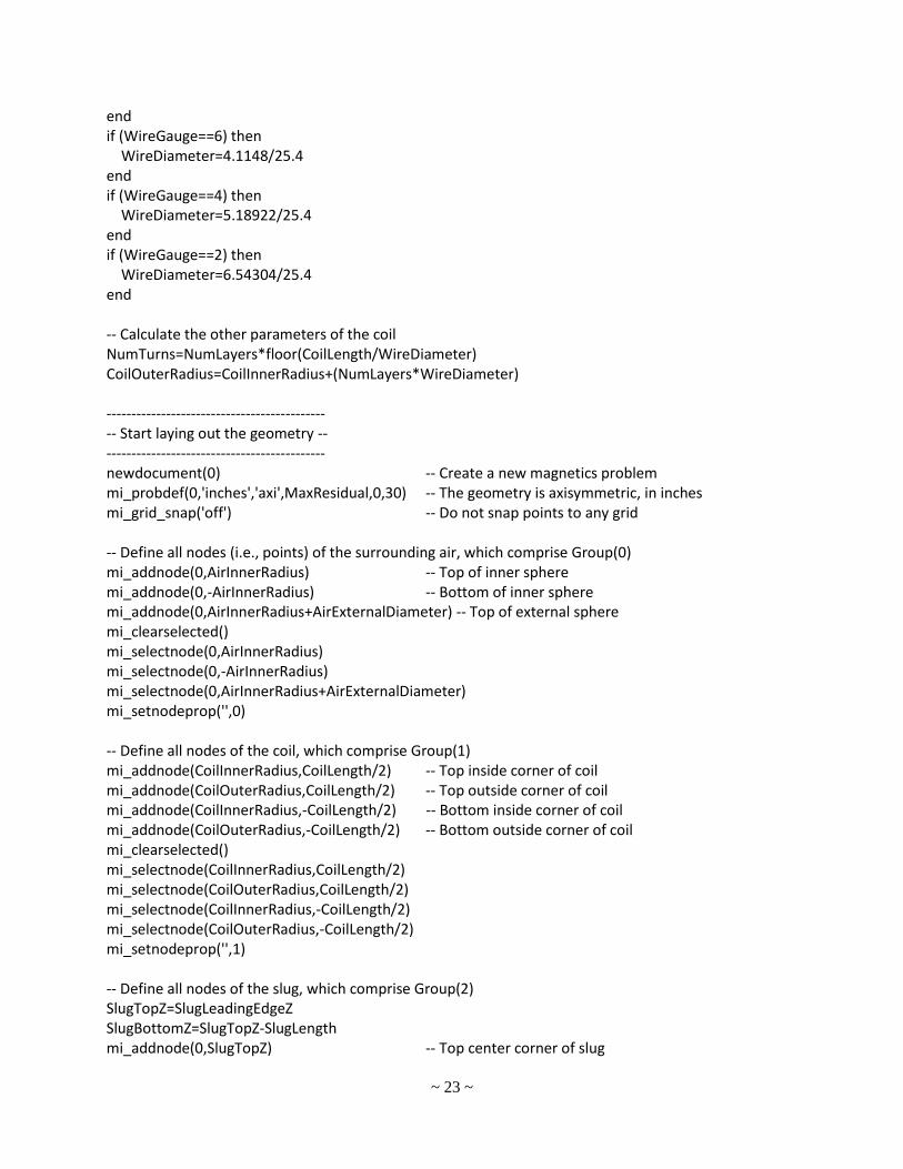
~ 23 ~

end if (WireGauge==6) then WireDiameter=4.1148/25.4 end if (WireGauge==4) then WireDiameter=5.18922/25.4 end if (WireGauge==2) then WireDiameter=6.54304/25.4 end -- Calculate the other parameters of the coil NumTurns=NumLayers*floor(CoilLength/WireDiameter) CoilOuterRadius=CoilInnerRadius+(NumLayers*WireDiameter) -------------------------------------------- -- Start laying out the geometry -- -------------------------------------------- newdocument(0) -- Create a new magnetics problem mi_probdef(0,'inches','axi',MaxResidual,0,30) -- The geometry is axisymmetric, in inches mi_grid_snap('off') -- Do not snap points to any grid -- Define all nodes (i.e., points) of the surrounding air, which comprise Group(0) mi_addnode(0,AirInnerRadius) -- Top of inner sphere mi_addnode(0,-AirInnerRadius) -- Bottom of inner sphere mi_addnode(0,AirInnerRadius+AirExternalDiameter) -- Top of external sphere mi_clearselected() mi_selectnode(0,AirInnerRadius) mi_selectnode(0,-AirInnerRadius) mi_selectnode(0,AirInnerRadius+AirExternalDiameter) mi_setnodeprop('',0) -- Define all nodes of the coil, which comprise Group(1) mi_addnode(CoilInnerRadius,CoilLength/2) -- Top inside corner of coil mi_addnode(CoilOuterRadius,CoilLength/2) -- Top outside corner of coil mi_addnode(CoilInnerRadius,-CoilLength/2) -- Bottom inside corner of coil mi_addnode(CoilOuterRadius,-CoilLength/2) -- Bottom outside corner of coil mi_clearselected() mi_selectnode(CoilInnerRadius,CoilLength/2) mi_selectnode(CoilOuterRadius,CoilLength/2) mi_selectnode(CoilInnerRadius,-CoilLength/2) mi_selectnode(CoilOuterRadius,-CoilLength/2) mi_setnodeprop('',1) -- Define all nodes of the slug, which comprise Group(2) SlugTopZ=SlugLeadingEdgeZ SlugBottomZ=SlugTopZ-SlugLength mi_addnode(0,SlugTopZ) -- Top center corner of slug

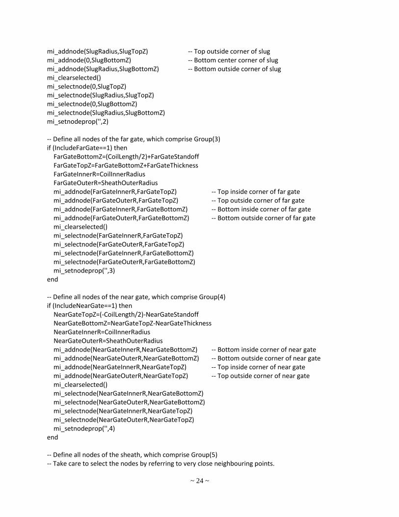
~ 24 ~

mi_addnode(SlugRadius,SlugTopZ) -- Top outside corner of slug mi_addnode(0,SlugBottomZ) -- Bottom center corner of slug mi_addnode(SlugRadius,SlugBottomZ) -- Bottom outside corner of slug mi_clearselected() mi_selectnode(0,SlugTopZ) mi_selectnode(SlugRadius,SlugTopZ) mi_selectnode(0,SlugBottomZ) mi_selectnode(SlugRadius,SlugBottomZ) mi_setnodeprop('',2) -- Define all nodes of the far gate, which comprise Group(3) if (IncludeFarGate==1) then FarGateBottomZ=(CoilLength/2)+FarGateStandoff FarGateTopZ=FarGateBottomZ+FarGateThickness FarGateInnerR=CoilInnerRadius FarGateOuterR=SheathOuterRadius mi_addnode(FarGateInnerR,FarGateTopZ) -- Top inside corner of far gate mi_addnode(FarGateOuterR,FarGateTopZ) -- Top outside corner of far gate mi_addnode(FarGateInnerR,FarGateBottomZ) -- Bottom inside corner of far gate mi_addnode(FarGateOuterR,FarGateBottomZ) -- Bottom outside corner of far gate mi_clearselected() mi_selectnode(FarGateInnerR,FarGateTopZ) mi_selectnode(FarGateOuterR,FarGateTopZ) mi_selectnode(FarGateInnerR,FarGateBottomZ) mi_selectnode(FarGateOuterR,FarGateBottomZ) mi_setnodeprop('',3) end -- Define all nodes of the near gate, which comprise Group(4) if (IncludeNearGate==1) then NearGateTopZ=(-CoilLength/2)-NearGateStandoff NearGateBottomZ=NearGateTopZ-NearGateThickness NearGateInnerR=CoilInnerRadius NearGateOuterR=SheathOuterRadius mi_addnode(NearGateInnerR,NearGateBottomZ) -- Bottom inside corner of near gate mi_addnode(NearGateOuterR,NearGateBottomZ) -- Bottom outside corner of near gate mi_addnode(NearGateInnerR,NearGateTopZ) -- Top inside corner of near gate mi_addnode(NearGateOuterR,NearGateTopZ) -- Top outside corner of near gate mi_clearselected() mi_selectnode(NearGateInnerR,NearGateBottomZ) mi_selectnode(NearGateOuterR,NearGateBottomZ) mi_selectnode(NearGateInnerR,NearGateTopZ) mi_selectnode(NearGateOuterR,NearGateTopZ) mi_setnodeprop('',4) end -- Define all nodes of the sheath, which comprise Group(5) -- Take care to select the nodes by referring to very close neighbouring points.

~ 25 ~

if (IncludeSheath==1) then if (IncludeFarGate==1) then SheathTopZ=FarGateBottomZ end if (IncludeFarGate==0) then SheathTopZ=(CoilLength/2)+PhenolicThickness+SheathFarExtension end mi_addnode(SheathInnerRadius,SheathTopZ) -- Top inside corner of sheath mi_addnode(SheathOuterRadius,SheathTopZ) -- Top outside corner of sheath if (IncludeNearGate==1) then SheathBottomZ=NearGateTopZ end if (IncludeNearGate==0) then SheathBottomZ=-((CoilLength/2)+PhenolicThickness+SheathNearExtension) end mi_addnode(SheathInnerRadius,SheathBottomZ) -- Bottom inside corner of sheath mi_addnode(SheathOuterRadius,SheathBottomZ) -- Bottom outside corner of sheath mi_clearselected() mi_selectnode(SheathInnerRadius,SheathTopZ-0.00001) mi_selectnode(SheathOuterRadius,SheathTopZ-0.00001) mi_selectnode(SheathInnerRadius,SheathBottomZ+0.00001) mi_selectnode(SheathOuterRadius,SheathBottomZ+0.00001) mi_setnodeprop('',5) end -- Define all segments (i.e., lines) of the surrounding air, which must be put into Group(0) -- There are three line segments: -- 1. From the bottom of the local sphere to the trailing edge of the slug. -- 2. From the leading edge of the slug to the top of the local sphere. -- 3. The diameter line across the external sphere. mi_addsegment(0,-AirInnerRadius,0,SlugBottomZ) mi_addsegment(0,SlugTopZ,0,AirInnerRadius) mi_addsegment(0,AirInnerRadius,0,AirInnerRadius+AirExternalDiameter) mi_clearselected() mi_selectsegment(0,-AirInnerRadius+0.00001) mi_selectsegment(0,AirInnerRadius-0.00001) mi_selectsegment(0,AirInnerRadius+0.00001) mi_setsegmentprop('',0,0,0,0) -- Define a periodic boundary condition mi_addboundprop('PeriodicBC',0,0,0,0,0,0,0,0,4) -- Define all arcs of the surrounding air, which must be put into Group(0) -- There are two arcs: -- 1. Enclosing the local sphere. -- 2. Enclosing the external sphere. mi_addarc(0,-AirInnerRadius,0,AirInnerRadius,180,1) mi_addarc(0,AirInnerRadius,0,AirInnerRadius+AirExternalDiameter,180,1)

~ 26 ~

mi_clearselected() mi_selectarcsegment(0,AirInnerRadius-0.00001) mi_selectarcsegment(0,AirInnerRadius+0.00001) mi_setarcsegmentprop(1,'PeriodicBC',0,0) -- Define all segments of the coil, which are in Group(1) -- The coil's cross-section is a simple rectangle, with four sides. mi_addsegment(CoilInnerRadius,-CoilLength/2,CoilInnerRadius,CoilLength/2) mi_addsegment(CoilInnerRadius,CoilLength/2,CoilOuterRadius,CoilLength/2) mi_addsegment(CoilOuterRadius,CoilLength/2,CoilOuterRadius,-CoilLength/2) mi_addsegment(CoilOuterRadius,-CoilLength/2,CoilInnerRadius,-CoilLength/2) mi_clearselected() mi_selectsegment((CoilInnerRadius+CoilOuterRadius)/2,CoilLength/2) mi_selectsegment((CoilInnerRadius+CoilOuterRadius)/2,-CoilLength/2) mi_selectsegment(CoilInnerRadius,0) mi_selectsegment(CoilOuterRadius,0) mi_setsegmentprop('',0,0,0,1) -- Define all segments of the slug, which are in Group(2) -- The slug's cross-section is a simple rectangle, with four sides. mi_addsegment(0,SlugBottomZ,0,SlugTopZ) mi_addsegment(0,SlugTopZ,SlugRadius,SlugTopZ) mi_addsegment(SlugRadius,SlugTopZ,SlugRadius,SlugBottomZ) mi_addsegment(SlugRadius,SlugBottomZ,0,SlugBottomZ) mi_clearselected() mi_selectsegment(SlugRadius/2,SlugTopZ) mi_selectsegment(SlugRadius/2,SlugBottomZ) mi_selectsegment(0,(SlugTopZ+SlugBottomZ)/2) mi_selectsegment(SlugRadius,(SlugTopZ+SlugBottomZ)/2) mi_setsegmentprop('',0,0,0,2) -- Define all segments of the far gate, which are in Group(3) -- The far gate's cross-section is a simple rectangle, with four sides. if (IncludeFarGate==1) then mi_addsegment(FarGateInnerR,FarGateBottomZ,FarGateInnerR,FarGateTopZ) mi_addsegment(FarGateInnerR,FarGateTopZ,FarGateOuterR,FarGateTopZ) mi_addsegment(FarGateOuterR,FarGateTopZ,FarGateOuterR,FarGateBottomZ) mi_addsegment(FarGateOuterR,FarGateBottomZ,FarGateInnerR,FarGateBottomZ) mi_clearselected() mi_selectsegment(FarGateInnerR+0.00001,FarGateTopZ) mi_selectsegment(FarGateInnerR+0.00001,FarGateBottomZ) mi_selectsegment(FarGateInnerR,(FarGateTopZ+FarGateBottomZ)/2) mi_selectsegment(FarGateOuterR,(FarGateTopZ+FarGateBottomZ)/2) mi_setsegmentprop('',0,0,0,3) end -- Define all segments of the near gate, which are in Group(4) -- The near gate's cross-section is a simple rectangle, with four sides.

~ 27 ~

if (IncludeNearGate==1) then mi_addsegment(NearGateInnerR,NearGateBottomZ,NearGateInnerR,NearGateTopZ) mi_addsegment(NearGateInnerR,NearGateTopZ,NearGateOuterR,NearGateTopZ) mi_addsegment(NearGateOuterR,NearGateTopZ,NearGateOuterR,NearGateBottomZ) mi_addsegment(NearGateOuterR,NearGateBottomZ,NearGateInnerR,NearGateBottomZ) mi_clearselected() mi_selectsegment(NearGateInnerR+0.00001,NearGateTopZ) mi_selectsegment(NearGateInnerR+0.00001,NearGateBottomZ) mi_selectsegment(NearGateInnerR,(NearGateTopZ+NearGateBottomZ)/2) mi_selectsegment(NearGateOuterR,(NearGateTopZ+NearGateBottomZ)/2) mi_setsegmentprop('',0,0,0,4) end -- Define all segments of the sheath, which must be put into Group(5) -- The sheath's cross-section is a simple rectangle, with four sides. if (IncludeSheath==1) then mi_addsegment(SheathInnerRadius,SheathBottomZ,SheathInnerRadius,SheathTopZ) mi_addsegment(SheathInnerRadius,SheathTopZ,SheathOuterRadius,SheathTopZ) mi_addsegment(SheathOuterRadius,SheathTopZ,SheathOuterRadius,SheathBottomZ) mi_addsegment(SheathOuterRadius,SheathBottomZ,SheathInnerRadius,SheathBottomZ) mi_clearselected() mi_selectsegment((SheathInnerRadius+SheathOuterRadius)/2,SheathTopZ-0.00001) mi_selectsegment((SheathInnerRadius+SheathOuterRadius)/2,SheathBottomZ+0.00001) mi_selectsegment(SheathInnerRadius,0) mi_selectsegment(SheathOuterRadius,0) mi_setsegmentprop('',0,0,0,5) end -- Define all block labels of the air, which must be put into Group(0) mi_addblocklabel(AirInnerRadius/2,AirInnerRadius/2) mi_addblocklabel(AirExternalDiameter/4,AirInnerRadius+(AirExternalDiameter/2)) mi_clearselected() mi_selectlabel(AirInnerRadius/2,AirInnerRadius/2) mi_selectlabel(AirExternalDiameter/4,AirInnerRadius+(AirExternalDiameter/2)) mi_getmaterial('Air') mi_setblockprop('Air',0,0,0,0,0,0) -- Describe the external region as a Kelvin transformation mi_defineouterspace(AirInnerRadius+(AirExternalDiameter/2),AirExternalDiameter/2,AirInnerRadius) -- Temporarily define a new material for the wire being used. This is done so that the user -- does not have to manually add a wire to the FEMM's default materials library. -- Name = TempWire -- Relative permeability in r-direction = 1 -- Relative permeability in z-direction = 1 -- Permanent magnet coercivity = 0 -- Applied source current density = 0 -- Electrical conductivity = 58 MS/m

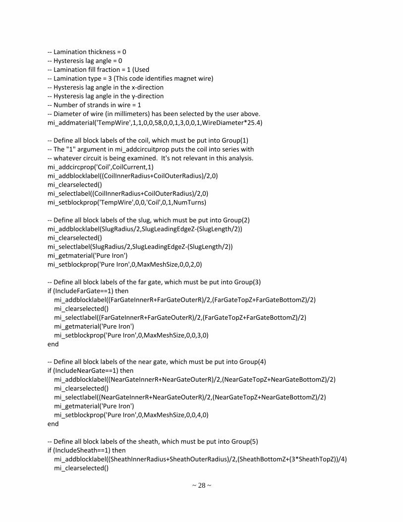
~ 28 ~

-- Lamination thickness = 0 -- Hysteresis lag angle = 0 -- Lamination fill fraction = 1 (Used -- Lamination type = 3 (This code identifies magnet wire) -- Hysteresis lag angle in the x-direction -- Hysteresis lag angle in the y-direction -- Number of strands in wire = 1 -- Diameter of wire (in millimeters) has been selected by the user above. mi_addmaterial('TempWire',1,1,0,0,58,0,0,1,3,0,0,1,WireDiameter*25.4) -- Define all block labels of the coil, which must be put into Group(1) -- The "1" argument in mi_addcircuitprop puts the coil into series with -- whatever circuit is being examined. It's not relevant in this analysis. mi_addcircprop('Coil',CoilCurrent,1) mi_addblocklabel((CoilInnerRadius+CoilOuterRadius)/2,0) mi_clearselected() mi_selectlabel((CoilInnerRadius+CoilOuterRadius)/2,0) mi_setblockprop('TempWire',0,0,'Coil',0,1,NumTurns) -- Define all block labels of the slug, which must be put into Group(2) mi_addblocklabel(SlugRadius/2,SlugLeadingEdgeZ-(SlugLength/2)) mi_clearselected() mi_selectlabel(SlugRadius/2,SlugLeadingEdgeZ-(SlugLength/2)) mi_getmaterial('Pure Iron') mi_setblockprop('Pure Iron',0,MaxMeshSize,0,0,2,0) -- Define all block labels of the far gate, which must be put into Group(3) if (IncludeFarGate==1) then mi_addblocklabel((FarGateInnerR+FarGateOuterR)/2,(FarGateTopZ+FarGateBottomZ)/2) mi_clearselected() mi_selectlabel((FarGateInnerR+FarGateOuterR)/2,(FarGateTopZ+FarGateBottomZ)/2) mi_getmaterial('Pure Iron') mi_setblockprop('Pure Iron',0,MaxMeshSize,0,0,3,0) end -- Define all block labels of the near gate, which must be put into Group(4) if (IncludeNearGate==1) then mi_addblocklabel((NearGateInnerR+NearGateOuterR)/2,(NearGateTopZ+NearGateBottomZ)/2) mi_clearselected() mi_selectlabel((NearGateInnerR+NearGateOuterR)/2,(NearGateTopZ+NearGateBottomZ)/2) mi_getmaterial('Pure Iron') mi_setblockprop('Pure Iron',0,MaxMeshSize,0,0,4,0) end -- Define all block labels of the sheath, which must be put into Group(5) if (IncludeSheath==1) then mi_addblocklabel((SheathInnerRadius+SheathOuterRadius)/2,(SheathBottomZ+(3*SheathTopZ))/4) mi_clearselected()

~ 29 ~

mi_selectlabel((SheathInnerRadius+SheathOuterRadius)/2,(SheathBottomZ+(3*SheathTopZ))/4) mi_getmaterial('Pure Iron') mi_setblockprop('Pure Iron',0,MaxMeshSize,0,0,5,0) end -- Save the construction in a temporary file which is a sister file to this Lua script. mi_saveas("./temp.fem") --************************************************************************************ --** All of the code up to this point is exactly the same as it was in the Lua script --** listed in Appendix "A" of an earlier paper titled "Using FEMM to analyze a coil --** from a coil gun", except for setting the maximum mesh size and precision. --************************************************************************************ -- Set the component values Cap = 0.016 -- Ideal capacitance, in Farads Resr = 0.038654 -- Capacitor's ESR, in Ohms Rcoil = 0.05955534 -- Ohmic resistance of coil, in Ohms Rhook = 0.004014 -- Resistance of hookup wire, in Ohms Rscr = 0.0015 -- On-resistance of SCR, in Ohms Rfixed = Rcoil + Rhook + Rscr + Resr -- Set the initial conditions; leave the slug where it was when we built the geometry VCap_0 = 390 -- Capacitor is charged up to 390V I_0 = 0 -- No current flowing -- Definition of electrical variables at the start and end of a time step -- QCap_start -- Charge stored in the ideal capacitor, in Coulombs -- QCap_end -- I_start -- Current, in Amperes -- I_end -- dIdt_constant -- First derivative of current at start of time step -- LTotal_start -- Total inductance at start of time step, in Henries -- LCoil -- (Constant) inductance of the coil, in Henries -- LSlug_start -- Additional inductance due to the slug, in Henries -- dLslugdI_start -- Partial derivative of Lslug w.r.t. current -- VCap_start -- Voltage drop over the ideal capacitor -- VCap_end -- Definition of fixed resistance voltage drops, in Volts, at the end of time step -- V_Resr -- Voltage drop over capacitor's ESR -- V_Rcoil -- Voltage drop over coil's Ohmic resistance -- V_Rhook -- Voltage drop over the hookup wire -- V_Rscr -- Voltage drop over the SCR -- Definition of energies, in Joules -- deltaH -- Heat burned off by fixed resistors during one time step -- EHeat_end -- Cumulative heat burned off, at end of time step

~ 30 ~

-- ECap_end -- Electrical energy stored in ideal capacitor, at end of time step -- ECoil_end -- Magnetic energy stored in ideal coil, at end of time step -- ESlug_end -- Magnetic energy stored in slug, at end of time step -- EnergyTotal -- Total system energy, at end of time step -- EnergyError -- Difference between total system energy and initial energy -- Variables related to the simulation process deltaT = 0.000001 -- The duration of one time step, in seconds SaveInterval = 1 -- Save results to file after this number of time steps SaveCounter = 0 -- Counter of time steps between save events MaxNumTimeSteps = 10000 -- Maximum number of time steps permitted -- As a preliminary step, let's calculate the inductance of the coil while the slug -- is in its fixed position. Note that the value for current specified in function -- modifycuircuitprop() cannot be zero. We will set it to something small. mi_modifycircprop('Coil',1,0.000000000001) mi_analyze() mi_loadsolution() val1,val2,val3 = mo_getcircuitproperties('Coil') LCoil = val3 / val1 -- Set all variables to their values at the end of time step #0, i.e., at Time=0 VCap_end = VCap_0 QCap_end = Cap * VCap_0 I_end = 0 EHeat_end = 0 ECap_end = 0.5 * Cap * VCap_0 * VCap_0 ECoil_end = 0 ESlug_end = 0 EHeat_end = 0 EnergyTotal_0 = ECap_end -- Open the text file for output and write a short header handle = openfile("./Coil_Gun_Stationary_slug.txt","a") write(handle,"Stationary slug with:\n") write(handle," TimeStep = ",deltaT * 1000000," micro-seconds\n") write(handle," Capacitor voltage = ",VCap_0," Volts\n") write(handle," Slug's LE location = ",SlugLeadingEdgeZ," inches\n") write(handle," Wire gauge = ",WireGauge,"\n") write(handle," Number of layers = ",NumLayers,"\n") write(handle," FEMM maximum mesh size = ",MaxMeshSize,"\n") write(handle," FEMM maximum residual = ",MaxResidual,"\n") -- Write headers for the columns of numbers in the output text file write(handle," Time LCoil LSlug dLSlug/dI Q_Cap V_Cap I") write(handle," ECap ECoil Slug EHeat ETotal EError\n") write(handle,"(usec) (uH) (uH) (uH/A) (C) (V) (A)") write(handle," (J) (J) (J) (J) (J) (J)\n")

~ 31 ~

-- Write the starting values write(handle,format("%6.1f ",0)) write(handle,format("%10.6f ",LCoil * 1000000)) write(handle,format("%10.6f ",0)) write(handle,format("%10.6f ",0)) write(handle,format("%8.6f ",QCap_end)) write(handle,format("%6.2f ",VCap_end)) write(handle,format("%8.2f ",I_end)) write(handle,format("%9.4f ",ECap_end)) write(handle,format("%9.4f ",ECoil_end)) write(handle,format("%9.4f ",ESlug_end)) write(handle,format("%9.4f ",EHeat_end)) write(handle,format("%9.4f ",EnergyTotal_0)) write(handle,format("%9.4f \n",0)) SaveCounter = 0 -- Set the screen display as desired main_maximize() -- Maximize the main FEMM window mi_zoomnatural() -- Scale the display to show the complete configuration showconsole() -- Show the Lua output window clearconsole() -- Clear the Lua output window --------------------------------- -- Begin the simulation -- --------------------------------- -- Main loop through time steps for TimeStep = 1,MaxNumTimeSteps do Time = TimeStep * deltaT -- Step #1: Bring forward the values from the end of the previous time step QCap_start = QCap_end I_start = I_end VCap_start = VCap_end -- Step #2A: Use FEMM to calculate the inductance if (abs(I_start) < 0.000000000001) then mi_modifycircprop('Coil',1,0.000000000001) else mi_modifycircprop('Coil',1,abs(I_start)) end mi_analyze() mi_loadsolution() val1,val2,val3 = mo_getcircuitproperties('Coil') LTotal_start = val3 / val1 LSlug_start = LTotal_start - LCoil -- Step #2B: Use FEMM to calculate the partial derivative dLSlug/dI

~ 32 ~

mi_modifycircprop('Coil',1,abs(I_start + 10)) mi_analyze() mi_loadsolution() val1,val2,val3 = mo_getcircuitproperties('Coil') LTotal_differentCurrent = val3 / val1 dLSlugdI_start = (LTotal_differentCurrent - LTotal_start)/10 -- Step #3: Calculate the derivative dI/dt_start Denominator = LCoil + LSlug_start + (I_start * dLSlugdI_start) if (TimeStep == 1) then dIdt_constant = (1/Denominator) * (QCap_start / Cap) else dIdt_constant = (1/Denominator) *((-Rfixed * I_start) + (QCap_start / Cap)) end -- Step #4: Integrate twice I_end = I_start + (dIdt_constant * deltaT) QCap_end = QCap_start + (-I_start * deltaT) + (-0.5 * dIdt_constant * deltaT * deltaT) -- Step #5: Calculate the ending voltage drop over the ideal capacitor VCap_end = QCap_end / Cap -- Step #6: Calculate the heat burned off by the fixed resistors deltaH = Rfixed * deltaT * ( (I_start * I_start) + (I_start * dIdt_constant * deltaT) + ((1/3) * dIdt_constant * dIdt_constant * deltaT * deltaT) ) EHeat_end = EHeat_end + deltaH -- Step #7: Calculate the electrostatic energy stored in the ideal capacitor ECap_end = 0.5 * Cap * VCap_end * VCap_end -- Step #8: Calculate the magnetic energy stored in the ideal coil ECoil_end = 0.5 * LCoil * I_end * I_end -- Step #9: Calculate the magnetic energy stored in the slug ESlug_end = (0.5 * LSlug_start * I_end * I_end) + ((1/3) * dLSlugdI_start * I_end * I_end * I_end) -- Step #10: Calculate the system total energies EnergyTotal = EHeat_end + ECap_end + ECoil_end + ESlug_end EnergyError = EnergyTotal - EnergyTotal_0 -- Step #11: Write the results to the output text file SaveCounter = SaveCounter + 1

~ 33 ~

if (SaveCounter >= SaveInterval) then SaveCounter = 0 write(handle,format("%6.1f ",Time * 1000000)) write(handle,format("%10.6f ",LCoil * 1000000)) write(handle,format("%10.6f ",LSlug_start * 1000000)) write(handle,format("%10.6f ",dLSlugdI_start * 1000000)) write(handle,format("%8.6f ",QCap_end)) write(handle,format("%6.2f ",VCap_end)) write(handle,format("%8.2f ",I_end)) write(handle,format("%9.4f ",ECap_end)) write(handle,format("%9.4f ",ECoil_end)) write(handle,format("%9.4f ",ESlug_end)) write(handle,format("%9.4f ",EHeat_end)) write(handle,format("%9.4f ",EnergyTotal)) write(handle,format("%9.4f \n",EnergyError)) end -- Step #12: Terminate the run when the current is less than one Ampere if ((TimeStep > 10) and (I_end < 1)) then TimeStep = MaxNumTimeSteps + 1 end -- Step #13: Display a message to the user in the Lua window print("Time (us) = ", Time * 1000000) print("LSlug_start (uH) = ", LSlug_start*1000000) print("dLSlug/dI_start (uH/A) = ", dLSlugdI_start*1000000) print("I (A) = ",I_start) end -- It is not necessary to remove the temporary wire material from the materials library, but -- removal can be done by uncommenting the following statement by removing the leading "--". -- mi_deletematerial('TempWire') -- Close out the Lua program closefile(handle) mo_close() mi_close() messagebox("All done.")