Aalborg Universitet

Using deep learning and meteorological parameters to forecast the photovoltaicgenerators intra-hour output power interval for smart grid control

Rodríguez, Fermín; Galarza, Ainhoa; Vasquez, Juan C.; Guerrero, Josep M.

Published in:Energy

DOI (link to publication from Publisher):10.1016/j.energy.2021.122116

Creative Commons LicenseCC BY-NC-ND 4.0

Publication date:2022

Document VersionPublisher's PDF, also known as Version of record

Link to publication from Aalborg University

Citation for published version (APA):Rodríguez, F., Galarza, A., Vasquez, J. C., & Guerrero, J. M. (2022). Using deep learning and meteorologicalparameters to forecast the photovoltaic generators intra-hour output power interval for smart grid control.Energy, 239, [122116]. https://doi.org/10.1016/j.energy.2021.122116

General rightsCopyright and moral rights for the publications made accessible in the public portal are retained by the authors and/or other copyright ownersand it is a condition of accessing publications that users recognise and abide by the legal requirements associated with these rights.

? Users may download and print one copy of any publication from the public portal for the purpose of private study or research. ? You may not further distribute the material or use it for any profit-making activity or commercial gain ? You may freely distribute the URL identifying the publication in the public portal ?

Take down policyIf you believe that this document breaches copyright please contact us at vbn@aub.aau.dk providing details, and we will remove access tothe work immediately and investigate your claim.

lable at ScienceDirect

Energy 239 (2022) 122116

Contents lists avai

Energy

journal homepage: www.elsevier .com/locate/energy

Using deep learning and meteorological parameters to forecast thephotovoltaic generators intra-hour output power interval for smartgrid control

Fermín Rodríguez a, b, *, Ainhoa Galarza a, b, Juan C. Vasquez c, Josep M. Guerrero c

a Ceit-Basque Research and Technology Alliance (BRTA), Manuel Lardizabal 15, 20018, Donostia\San Sebasti�an, Spainb Universidad de Navarra, Tecnun, Manuel Lardizabal 13, 20018, Donostia/San Sebasti�an, Spainc Center for Research on Microgrids (CROM), Department of Energy Technology, Aalborg University, Aalborg, 9220, Denmark

a r t i c l e i n f o

Article history:Received 9 February 2021Received in revised form17 September 2021Accepted 18 September 2021Available online 24 September 2021

Keywords:Confidence interval forecastIntra-hour horizonSolar irradiationSmart controlPhotovoltaic generation output power

* Corresponding author. Ceit-Basque Research andManuel Lardizabal 15, 20018, Donostia\San Sebasti�an

E-mail address: frlalanne@ceit.es (F. Rodríguez).

https://doi.org/10.1016/j.energy.2021.1221160360-5442/© 2021 The Author(s). Published by Elsevie).

a b s t r a c t

In recent years, the photovoltaic generation installed capacity has been steadily growing thanks to itsinexhaustible and non-polluting characteristics. However, solar generators are strongly dependent onintermittent weather parameters, increasing power systems' uncertainty level. Forecasting models havearisen as a feasible solution to decreasing photovoltaic generators' uncertainty level, as they can produceaccurate predictions. Traditionally, the vast majority of research studies have focused on the develop-ment of accurate prediction point forecasters. However, in recent years some researchers have suggestedthe concept of prediction interval forecasting, where not only an accurate prediction point but also theconfidence level of a given prediction are computed to provide further information. This paper develops anewmodel for predicting photovoltaic generators' output power confidence interval 10 min ahead, basedon deep learning, mathematical probability density functions and meteorological parameters. Themodel's accuracy has been validated with a real data series collected from Spanish meteorological sta-tions. In addition, two error metrics, prediction interval coverage percentage and Skill score, arecomputed at a 95% confidence level to examine the model's accuracy. The prediction interval coveragepercentage values are greater than the chosen confidence level, which means, as stated in the literature,the proposed model is well-founded.© 2021 The Author(s). Published by Elsevier Ltd. This is an open access article under the CC BY-NC-ND

license (http://creativecommons.org/licenses/by-nc-nd/4.0/).

1. Introduction

Renewable energies have arisen as feasible alternatives toexhaustible fossil energies and a way to reduce greenhouse emis-sions such as CO2 and NOX [1]. For instance, the German govern-ment, following European goals for energy transition, has fixedshort and long term milestones in order to replace fossil resourceswith renewable ones. Thus, the share of renewables in the Germanelectric generation matrix must be 20%, 30% and 63% by the end ofyears 2020, 2025 and 2050, respectively [2]. In order to achieve thestated milestones and support the introduction of renewable gen-erators into the traditional grid, laws were adopted to guaranteerenewable plants' profits. Hence, between 2002 and 2017, the

Technology Alliance (BRTA),, Spain.

r Ltd. This is an open access article

installed renewable energy capacity increased 516.67%, i.e. from18 GW to 111 GW in Germany [3]. This positive trend in installedrenewable capacity is also found in other countries, and it is ex-pected to continue in upcoming years [4,5]. However, not allrenewable energies have had the same evolution, with solarphotovoltaic (PV) and wind technologies being the most widelyinstalled, not only for large scale generators [6] but also in theresidential sector, in case of PV generators [7].

Although renewable technologies, and particularly PV genera-tors, are essential for energy transition, it must also be kept in mindthat they will be connected to traditional grids. Such networkswere linearly structured in that different stakeholders, i.e. genera-tors, transmission system operators, distribution system operatorsand customers, hadwell-defined tasks and operating requirements.However, small-scale PV systems are strongly dependent onintermittent, volatile and random meteorological parameters, suchas solar irradiation intensity or the cloud effect, making themgenerators with high levels of uncertainty [8,9]. Large-scale PV

under the CC BY-NC-ND license (http://creativecommons.org/licenses/by-nc-nd/4.0/

List of abbreviations

Notation DescriptionANN Artificial Neural NetworkARMA Autoregressive Moving AverageARIMA Autoregressive Integrated Moving Averagebn Bias value of the n-th neuronDL Deep LearningDPI Direct Prediction IntervalI Hidden NeuronsIPI Indirect Prediction IntervalJðbgÞ Jacobian MatrixL Recent past deviationsLBa Lower Bound for a chosen a

ML Machine LearningNPPI Non-Parametric Prediction IntervalP Input ParametersPDF Probability Distribution FunctionPI Prediction IntervalPICP Prediction Interval Coverage Percentage

PP Prediction PointPPI Parametric Prediction IntervalPV Photovoltaic

Gradient vectorSSN Skill Score NormalizedSTFFNN Spatiotemporal Feedforward Neural Networku2 Unbiased estimatorUBa Upper Bound for a chosen a

wp;i Weights of the n-th neuronxi Input vector of the n-th neurony Actual valueby Predicted valuea Error rate chosen by the userε Approximation errorg Set of parameters that model the ANNg* Optimal set of parametersbg Least squares estimator of f*

s2 Variance

F. Rodríguez, A. Galarza, J.C. Vasquez et al. Energy 239 (2022) 122116

generators are less affected by punctual effects such as cloudsmovement and have a more stable behaviour. This uncertaintygenerates unexpected and sudden changes in PV systems' outputpower, thereby hindering power system operation, and as a resultthe spread of renewable generators in traditional grids is limited[10]. Therefore, it must be ensured that increasing renewable ca-pacity will not negatively affect power system security and stabilityin operating conditions [11].

Historically, reversible hydropower plants aside, electric storagedevices were not developed for accumulating too much energy.Therefore, electric power systems' decisionmakers guaranteed gridstability through real-time balancing actions with regard to energydemand and energy generation, along with some energy demandforecasts for different prediction horizons [12,13]. Some of the mostrelevant tasks that power system decision makers perform are:real-time control, unit commitment or economic dispatch, as wellas maintenance scheduling [13,14]. When large and small scale PVgenerators were introduced into the traditional grid, the uncer-tainty level of whole power systems increased due to the aboveexplained characteristics of renewable energies. To address thissituation, renewable energy generation forecasters emerged as afeasible and effective solution [15].

Due to the wide variety of activities realized by power systemdecision makers, researchers developed different forecasters,attending to each activity's prediction horizon requirements. Interms of prediction horizon, renewable forecasters are classifiedinto the following main groups [16]:

� Intra-hour prediction horizon forecasters: also called now-casting in the literature [17,18], compute predictions for thedesired parameters, going from 1 min to an hour ahead [19].These forecasters are commonly used in real-time dispatch ac-tivities by power system decision makers to keep traditionalgrids within safe operating requirements [20].

� Intra-day prediction horizon forecaster: the literature agreeson fixing a horizon range from one to 6 h ahead [21,22]. Thus,forecast values are used by power system decision makers inintra-day energy markets for load trading proposes in order toensure grid stability [23].

2

� Day-ahead prediction horizon forecasters: the literatureagrees on classifying in this group forecasters whose predictionhorizon is between six and 72 h or beyond [24,25]. Forecasterswith day-ahead or longer prediction horizons are usually char-acterized by an hourly resolution to increase the quality of theinformation provided [26]. Decision makers use the informationprovided by these forecasters for economic dispatch and unitcommitment optimization activities [27,28].

Some studies from the available literature [29e31] state thatrenewable generators' control strategies must be improved bydeveloping accurate forecasters in all the described predictionhorizons, making them more reliable for decision makers. Inaddition, although up to this moment renewable generators onlyprovide power to the main grid, the European Commission and theInternational Renewable Energy Agency have started suggestingthat renewable generators also provide ancillary services to themain grid [32,33]. Ancillary services can be defined as a set of ac-tivities that other stakeholders require from power systems' deci-sion makers in order to keep the traditional grid within stableoperating boundary conditions, such as frequency and voltage levelboundaries [34]. These services are currently provided by tradi-tional generators due to their relevance to power system operation,as well as their quicker capacity to change to the set up pointrequired by power system decision makers. Therefore, highly ac-curate intra-hour forecasters will need to be developed in order toallow renewable generators to provide these services [29].

Related to PV energy, the literature agrees that solar irradiation,outdoor temperature and wind speed are the most relevantmeteorological parameters involved in power production [35e37].These parameters not only affect the power PVs generate but alsothe generators' control parameters such as open voltage circuit,short circuit current and cell temperature [35]. However, of theabove listed meteorological parameters, several research studieshave demonstrated that solar irradiation has the strongest effect onPV generators' output power [22,35,36]. This is the reason whyhistorically the vast majority of research studies have been focusedon predicting the meteorological parameter of solar irradiation forall prediction horizons [3,8,14,19,29,31].

The first solar irradiation forecasters developed to address the

F. Rodríguez, A. Galarza, J.C. Vasquez et al. Energy 239 (2022) 122116

high uncertainty level of PV generators output power were pointprediction (PP) forecasters, which were classified as physical orstatistical forecasters [38]. Physical forecasters are characterized bythe application of weather phenomenon equations [39] andsometimes combined with sky imagery [40] or satellite devices[41], whereas statistical forecasters are based on the combination ofhistorical databases and machine learning (ML) algorithms forregression and feature selection proposes, such as lasso [42,43]algorithms. Physical forecasters are usually less studied due to theexpensive equipment and complex mathematical models required.ML statistical forecasters, also noted in the literature as autore-gressive models, are based on iterative correlation analyses to fixoptimal relationships between forecasters' input and output pa-rameters. Although autoregressive forecasters were acceptable inthe first steps in solar irradiation forecasting, their main drawbackwas their weak capacity to make accurate predictions whencommonly unexpected changes occur in solar irradiation values[44e46]. Autoregressive moving average (ARMA) [45] and autore-gressive integrated moving average (ARIMA) [46] forecasters aresome examples of the first ML forecasters.

To solve the ML forecasters' lack of capacity to predict suddenchanges, deep learning (DL) PP forecasters, which are also cata-logued as statistical forecasters, arose as a feasible solution. DLforecasters can be either combined with ML to overcome last ones'weakness or constitute as forecasters by themselves [44]. DL fore-casters try to emulate through mathematical approximations thehuman brain's capacity to learn from databases and produce pre-dictions based on previously unseen values [47]. Thus, DL fore-casters are commonly referred to as artificial neural networks(ANN) in the literature, and they have been used for various pur-poses, such as predicting parameters in different research areas[48,49], classification/pattern recognition studies [50] or serving asa baseline for new forecasters to improve forecaster accuracy[51,52].

Although the vast majority of researchers still focus onimproving the accuracy PP forecasters, some researchers such as Liet al. [53] and Liu et al. [54] have recently claimed that PP fore-casters do not provide complete information because they do notgive information about the deviation between actual and fore-casted values. In addition, both research studies [53,54] argued thatthe knowledge of boundaries around forecasted values will providerelevant information to power system decision makers to improvegrid stability and operating cost. Thus, prediction interval (PI)forecasters are starting to be developed not only to reducerenewable generator uncertainty [53,55] but also to provide moreinformation related to energy demand forecasting [36].

A literature review on PI forecasters suggests that these fore-casters can be classified according to two dimensions. The firstdimension examines whether the interval has been calculatedthrough a prediction made by a PP forecaster. Hence, indirectprediction interval (IPI) forecasters use values computed throughPP forecasters as a baseline [26,56], whereas direct prediction in-terval (DPI) forecasters do not use any baseline to compute theinterval [55,57]. Although there are few DPI forecasters, recentlyresearchers have examined them more widely. However, the vastmajority of researchers still prefer developing accurate PP fore-casters in order to develop through them IPI forecasters.

The second dimension examines whether researchers haveapproximated any parameters of the forecaster through a proba-bility density function (PDF). Forecasters which are based on thisPDF approximation are called parametric prediction interval (PPI)forecasters, whereas forecasters that are not based on PDF ap-proximations are known as non-parametric prediction interval

3

(NPPI) forecasters. PPI forecasters usually applied Normal, Gaussianor Laplacian [58,59] PDFs to describe the deviation between actualand forecasted values; these PDFs are then used to compute theinterval. However, recent NPPI research studies try to avoid thisapproximation, arguing that the assumption of describing param-eters through single or combined PDFs is speculative, inappropriateand not realistic [3,54,55]. Among all current NPPI forecastertechniques, quantile [54] and bootstrap [60] are the most widelyapplied ones.

This research paper presents a photovoltaic generator's outputpower intra-hour PI forecaster through meteorological parameters,specifically for 10 min ahead. Based on the classifications describedabove, the developed forecaster is catalogued as an indirect para-metric PI forecaster. It is indirect because the predicted solar irra-diation values obtained through a PP forecaster are used as abaseline to compute the PV generator's output power intervals, andit is parametric because the t-Student PDF has been used tocompute the error rate probability chosen by the user. The keycontributions of this research study are explained below:

1) A new intra-hour indirect parametric PI forecaster is proposedto estimate PV generator power output 10 min ahead. Thedeveloped model combines a DL model, specifically a feedfor-ward spatiotemporal neural network model (used as a baselinemodel), mathematical theorems and PDFs to compute the in-terval. The proposed PI forecaster's reliability has been testedwith real data series collected from meteorological stations inVitoria-Gasteiz, Spain.

2) PI forecaster accuracy is commonly studied through reliabilityand sharpness indexes. Different indexes, namely the predictioninterval coverage percentage (PICP) to examine the proposedforecaster's reliability and the Skill score to analyse thecomputed intervals width, were computed for 95% confidencelevel under sunny, partially cloudy and cloudy meteorologicalsituations. For the chosen confidence level, with the final fixedforecaster and under the different meteorological situationsexamined, the computed PICP value is higher than the selectedconfidence level. The literature agrees [36,59,61] that the PIforecaster model is valid when this situation occurs, and thusthe proposed forecaster is considered valid.

2. Methodology

To develop the PI forecaster proposed in this research study, a PPforecaster studied in a previous work is applied as a baseline [62].Both forecasters i.e. PI and PP forecasters, were developed withsame solar irradiation database. Table 1 describes the main char-acteristics of the PP forecaster, which is based on a DL spatiotem-poral feedfordward neural network (STFFNN), whereas Fig. 1presents the PP forecaster's layout. The STFFNN relies on thecombination of a DL feedforward neural network structure and themeteorological databases that contain information from the targetand surrounding meteorological stations.

As shown in Fig. 1, DL STFFNN forecasters are ANN structures,which rely on the combination of several parameters that arechosen through sensitivity analyses in order to obtain the best ac-curacy. Thus, some of the most relevant examined parameters are:the network's layers, each layer's number of neurons, each layer'sneuron activation function and learning algorithm.

For the STFFNN PP forecaster used as baseline, the outputcomputed at the hidden layer's i-th neuron is mathematicallydescribed as a linear combination of inputs, weights and biases

Table 1STFFNN PP baseline forecaster's main characteristics.

Input parameters (P) 1168 ¼ season (1), time (1) and solar irradiation data from target (144) and surrounding stations (1022)Output parameter solar irradiationNetwork structure Input e hidden e output layersHidden Neurons (I) 5Total amount of Weights (W) 5845Total amount of Biases (b) 6

Fig. 1. SPFFNN PP forecaster's layout.

F. Rodríguez, A. Galarza, J.C. Vasquez et al. Energy 239 (2022) 122116

applied in a sigmoidal activation function g:

gðxÞ¼ 11þ e�x (1)

xi ¼ f

0@ XP¼1168

p¼1

½w�p;i½j�p;1 þ bi

1A ; i2f1;2;…;5g (2)

where j2RP¼1168 is the input vector with 1168 dimensions, wp;i

refers to i-th neuron's weights with p2f1;2; …; 1168g, and birepresents i-th neuron's bias threshold value. In the same way, theoutput layer's neuron is mathematically described as a linearcombination of inputs, i.e. the hidden layer's neuron's outputvalues, weights and biases applied in a linear activation function:

by¼ XI¼5

i¼1

�wi;Iþ1

�½gðxiÞ� þ bIþ1: (3)

where by is not only the output value of the output layer's neuronbut also the STFFNN forecaster's predicted point value, which isused as a baseline to build up the PI forecaster.

2.1. Proposed PI methodology

Considering that solar PV generation mainly depends on solarirradiation, let's assume that this meteorological parameter'sbehaviour ðyÞ can be mathematically expressed as a combination ofan unknown scalar function ðzÞ and the parameters involved as

y¼ zðxÞ: (4)

Due to the complexity of developing an accurate physical fore-caster which describes solar irradiation behaviour ðzÞ, the aim is touse the STFFNN PP as an approximation of Eq. (4) in such away that

4

y¼hðx;g*Þ þ e: (5)

Where is defined as the difference between forecasted and actualvalues and ðg*Þ represents the most representative real set (R) ofparameters ðgÞ that better describe solar irradiation behaviour. Inaddition, selected real ðg*Þ parameters can be computed throughthe Levenberg-Marquardt algorithm, which is based on a leastsquares problem [63]. Thus, the STFFNN PP forecaster's predictedvalue ðbyÞ can be expressed as

by¼ hðx; bgÞ: (6)

Where ðbgÞ represents the computed ðg*Þ parameters computedthrough the Levenberg-Marquardt algorithm and function ðhÞ is theanalytical expression of the STFFNN PP forecaster described in Eq.(3).

Moreover, ðeÞ can also be mathematically described throughTaylor's first-order polynomial approximation combined with thetwo previously defined equations in such way that

e¼ y�hðx;g*Þz y�hðx; bgÞ� ðQðbgÞÞTðg*� bgÞ¼ y� by� ðg* � bgÞTQðbgÞ: (7)

Where QðbgÞ is h’s gradient, which is mathematically expressed as

QðbgÞ¼�vhðx; bgÞvbg1

;…;vhðx; bgÞvbgR

�T

(8)

Notice that terms in Eq. (7) can be rewritten in such way that

y� by¼ e� ðg* � bgÞTQðbgÞ: (9)

We assume that ðyÞ, ðbyÞ and ðeÞ behave as random variables andthat ðeÞ follows Nð0; s2Þ PDF and is independent from ðg* � bgÞ.Hence, Eq. (9) can bemathematically rewritten in root mean squareerror terms in such way that

F. Rodríguez, A. Galarza, J.C. Vasquez et al. Energy 239 (2022) 122116

Ehðy� byÞ2i¼ E

he2iþ ðQðbgÞÞTEhðbg�g*Þðbg � g*ÞT

iQðbgÞ: (10)

Where E is mathematically defined as expectation and the nextproperty can be used based on the previously explainedassumptions,

Ehðbg � g*ÞT ðbg�g*Þ

i¼s2

hJðbgÞT JðbgÞi�1

: (11)

Where JRxKðbgÞ is the Jacobian matrix where R is the number ofcolumns in the J matrix whose values are defined by g* number ofparameters and K is the number of rows in the J matrix whosevalues are defined by a set of samples of the database used in theforecaster's training step to compute bg. Combining the two equa-tions described above yields the following expression,

Ehðy� byÞ2i¼ s2

�1þðQðbgÞÞThJðbgÞT JðbgÞi�1

QðbgÞ�¼u2

�1þðQðbgÞÞThJðbgÞT JðbgÞi�1

QðbgÞ�¼ u2

�1þðQðbgÞÞTD�1QðbgÞ�

(12)

where u2 is defined as the s2 parameter's unbiased estimator,whose value is defined as,

u2 ¼ 1K � R

XKk¼1

ðyk � hðxk; bgÞÞ2: (13)

Observe that the unbiased estimator parameter, u2, can just becomputed if K >R; otherwise, the forecaster will not predict theinterval properly. This condition must also be taken into accountwhen the J matrix's dimensions are chosen. Finally, for sufficientnumber of K samples from the training database used to developthe baselinemodel, the random parameter T can bemathematicallydefined in such way that

T ¼ y� byu

ffiffiffiffiffiffiffiffiffiffiffiffiffiffiffiffiffiffiffiffiffiffiffiffiffiffiffiffiffiffiffiffiffiffiffiffiffiffiffiffiffiffiffiffiffi1þ ðQðbgÞÞTD�1QðbgÞq (14)

and whose behavior can be described by a Student's t-distributionPDF with K � R degrees of freedom [64]. Thus, the PI for estimationby obtained through the PP forecaster with confidence 100ð1�aÞ% iscomputed by

PI¼ by±ta=2R�Kuffiffiffiffiffiffiffiffiffiffiffiffiffiffiffiffiffiffiffiffiffiffiffiffiffiffiffiffiffiffiffiffiffiffiffiffiffiffiffiffiffiffiffiffiffi1þ ðQðbgÞÞTD�1QðbgÞq

: (15)

Where a2½0;1� represent the user's selected error rate, ta=2R�K ¼P�T < a

2

�and P refers to probability.

2.2. Benchmark model

To compare the results obtained by proposed PI forecaster in theabove section, the methodology proposed by Yan et al. [65] withsome modification has been computed as benchmark. In Ref. [65],Yan et al. proposed to compute the interval forecasting based onrecent deviations between actual and forecasted values combinedwith an ANN to predict future deviations. In a second step, futuredeviations are approximated through a Normal PDF to compute theintervals. Attending to the two criterion explained in Section 1, Yanet al.‘s methodology can be classified as indirect and parametric PI

5

forecaster; indirect because it applies a PP forecaster to computethe interval and parametric because Yan et al. approximated futuredeviations between actual and predicted values through a NormalPDF. Therefore, in Yan et al.‘s forecaster two parameters need to beselected: the error rate chosen by the end user a and the number ofrecent past deviations (L) that will be taken into account forcomputing the intervals. In this study, Yan et al. forecaster's secondstep was omitted, and the Normal PDF approximation was directlydone with previous deviations. Fig. 2 shows a layout about howcomputed benchmark model works.

2.3. PI forecasters error metrics

A literature review on PI forecaster accuracy error metrics sug-gests that these indexes are catalogued in two dimensions, reli-ability and sharpness metrics [26,36,53,58]. Reliability metricsexamine PI forecasters' accuracy, i.e., howmany of the actual valuesfall into forecasted intervals. Among all reliability metrics, predic-tion interval coverage percentage (PICP) is the most widelycomputed error metric [54,66]. Sharpness metrics analyse pre-dicted interval width, i.e., how close predicted interval's boundsare. In this study, a Skill score (SS) is computed to examine theproposed forecaster's sharpness.

By combining equations (6) and (15), the PI's lower bound (LB)and upper bound (UB) for a time instancem, ym can be expressed insuch way that,

LBaðxmÞ¼hðxm; bgÞ � ta=2R�Kuffiffiffiffiffiffiffiffiffiffiffiffiffiffiffiffiffiffiffiffiffiffiffiffiffiffiffiffiffiffiffiffiffiffiffiffiffiffiffiffiffiffiffiffiffi1þ ðQðbgÞÞTD�1QðbgÞq

; (16)

UBaðxmÞ¼hðxm; bgÞ þ ta=2R�Kuffiffiffiffiffiffiffiffiffiffiffiffiffiffiffiffiffiffiffiffiffiffiffiffiffiffiffiffiffiffiffiffiffiffiffiffiffiffiffiffiffiffiffiffiffi1þ ðQðbgÞÞTD�1QðbgÞq

: (17)

Once the PI's bounds are mathematically defined, PICP can bedescribed as,

PICPa ¼ 1M

XMm¼1

dam dam ¼(1; ym2PIam0; ym;PIam

: (18)

Where dam is a Boolean parameter which takes the value 1 if theactual value ym falls into the forecasted interval and the value 0 if itdoes not. M represents the number of samples examined. More-over, the condition PICPa >1� a must be met to consider the pro-posed PI forecaster as being suitable [54,66], otherwise theproposed forecaster needs to be examined until this condition ismet; 1� a value is also known as confidence level CLa.

To examine the predicted intervals for M actual values, the SSerror metric can be computed in such way that

SSa ¼ 1M

XMm¼1

dam �ð1�aÞmaxðjLBaðxmÞ� ymj; jym �UBaðxmÞjÞ

(19)

Eq. (19) demonstrates that in the SSa metric, the actual values ymthat fall into the PI have a lower penalty than when ym values fallout. In addition, SSa must always be positive and the closest the SSavalue is from zero, the better sharpness the PI has. Usually, the SSavalue is normalized through parameter N to make facilitate com-parison with other research studies in the literature,

SSNa ¼ 1NSSa: (20)

Fig. 2. Benchmark PI forecaster's layout.

F. Rodríguez, A. Galarza, J.C. Vasquez et al. Energy 239 (2022) 122116

3. Results

In this section, the proposed DL PI forecaster's accuracy isexamined. Our model predicts photovoltaic generators' outputpower interval through meteorological parameters, specificallythrough solar irradiation, for 10 min ahead. In order to make a realassessment, a solar irradiation database provided by Euskalmet, theBasque Government's Meteorological Agency (http://www.euskalmet.euskadi.eus/), is used. The selected solar irradiationdatabase has 10 min resolution and had to be the same as the oneused in the development of STFFNN forecaster. While the wholedatabase for years 2015e16 was used in the STFFNN forecaster'straining step, the entire database for year 2017 was used in theSTFFNN forecaster's validation [62]. Thus, in this study it was alsomandatory to use same databases, but for different purposes; the2015-16 database was applied to compute the Jacobian matrix JðbgÞ;whereas the 2017 database was applied to calculate the gradientvector QðbgÞ in (‘C040 Vitoria-Gasteiz, Spain’). Attending to K€oppen-Geiger climate classification, Vitoria-Gasteiz, Spain has an oceanicclimate, but at the same time is 60 km inland with yearly averagetemperature and precipitations of 11.4 �C and 782.3 mm,respectively.

3.1. Results of proposed solar irradiation PI forecaster

As explained above, the JðbgÞmatrix has R x K dimension and thecondition K >R must be satisfied to properly compute the u2 esti-mator (see Eq. (13)). Therefore, it is mandatory to first calculate Rparameter, which represents the set of parameters that describe theSTFFNN PP forecaster. Parameter R can be computed in such a waythat

R¼ IxðPþ2Þþ1¼W þ b¼5851: (21)

The second step consists of computing dimension K for matrixJðbgÞ in such a way that the proposed PI forecaster's accuracy is

6

maximized for solar irradiation forecasting 10 min ahead. For thispurpose, a sensitivity analysis was run, where in order to considerthe proposed PI forecaster acceptable, parameter K is varied untilthe condition PICPa > ð1�aÞ is achieved. Thus, dimension K of theJðbgÞ matrix must satisfy the following condition,105264>K >R ¼ 5851 where 105264 is the length of the trainingdatabase used to develop the PP baseline forecaster. Moreover,remember that, for the proposed algorithm for each examined Kset, parameters described in Eqs. (13)e(15) need to be calculated.To better examine the proposed solar irradiation PI forecaster,whole 2017 year was analysed, consisting of 72 sunny days, 47partially cloudy days and 246 cloudy days whose results are re-ported in Table 2. Noted that for each K set different analyses weredone; while “Global” makes reference to the error metrics forwhole days of 2017, there are also provided same error metric byeach type of day, i.e. sunny, partially cloudy or cloudy. Concerningthe error metrics presented in Table 2, %ðPICP>95Þ, gives in % for eachset of data the number of days that satisfied the conditionPICP>0:95; then for those days that satisfied the condition, PICP,sPICP, PICPMAX and PICPMIN indicate the mean average, the standarddeviation and the maximum and minimum values, respectively.M ¼ 144 represents the number of predicted values during eachday.

The results in Table 2 demonstrate that no matter which type ofday is being analysed (sunny, partially cloudy or cloudy), the lowerdimension K is, the higher the PICPa value is. This fact is related toDL overfitting phenomena, which is based on the fact that if toomuch similar data is used, the forecaster is not able to learn andinstead memorizes values, reducing its generalization capacity.

However, it can also be seen in Table 2 how there are someaccuracy differences depending on the type of day examined. Forinstance, for K ¼ 5974 and sunny days, 95.77% fulfil the conditionPICPa > ð1 � aÞ, whereas for the same K dimension and cloudydays, only 38.26% of the days fulfil the condition. In addition, it isalso necessary to examine the sharpness of the predicted intervals.

Table 2PICP0:05 results for solar irradiation PI forecasting.

Error metric K Analysis %ðPICP>95Þ PICP sPICP PICPMAX PICPMIN

100 � PICP (M ¼ 144) 6000 Global 43.48 97.54 1.52 100.00 95.14Sunny 95.77 98.35 1.33 100.00 95.14Partially Cloudy 77.27 97.06 1.22 99.31 95.14Cloudy 20.87 96.85 1.52 100.00 95.14

5974 Global 55.07 97.71 1.57 100.00 95.14Sunny 95.77 98.58 1.44 100.00 95.14Partially Cloudy 77.27 97.66 1.25 100.00 95.83Cloudy 38.26 97.91 1.46 100.00 95.14

5953 Global 73.33 97.88 1.58 100.00 95.14Sunny 98.59 99.09 1.10 100.00 95.14Partially Cloudy 90.91 98.09 1.33 100.00 95.14Cloudy 62.17 97.22 1.47 100.00 95.14

5943 Global 82.32 98.19 1.49 100.00 95.14Sunny 100.00 99.39 0.97 100.00 95.14Partially Cloudy 100.00 98.20 1.44 100.00 95.14Cloudy 73.48 97.67 1.39 100.00 95.14

5937 Global 85.22 98.25 1.54 100.00 95.14Sunny 100.00 99.47 0.88 100.00 95.14Partially Cloudy 100.00 98.45 1.41 100.00 95.14Cloudy 77.83 97.79 1.45 100.00 95.14

Table 3SSN0:05 results for solar irradiation PI forecasting for sunny days.

Error metric K Analysis SSN sSSN SSNMAX SSNMIN

100 � SSN (M ¼ 144) 6000 Global 2.29 1.70 7.93 0.45Sunny 1.28 0.64 2.98 0.45Partially Cloudy 2.09 1.04 4.00 0.70Cloudy 3.53 2.00 7.93 0.70

5974 Global 2.86 2.14 11.23 0.51Sunny 1.43 0.73 3.53 0.51Partially Cloudy 2.27 1.12 4.78 0.73Cloudy 4.16 2.14 11.23 0.79

5953 Global 3.36 2.33 11.13 0.58Sunny 1.63 0.87 4.22 0.58Partially Cloudy 2.50 1.34 6.20 0.86Cloudy 4.44 2.43 11.13 0.67

5943 Global 3.66 2.47 11.60 0.63Sunny 1.80 0.98 4.83 0.63Partially Cloudy 2.67 1.50 6.51 0.97Cloudy 4.70 2.54 11.60 0.63

5937 Global 3.74 2.50 11.27 0.63Sunny 1.88 1.04 5.10 0.66Partially Cloudy 2.74 1.58 6.92 0.98Cloudy 4.71 2.58 11.27 0.63

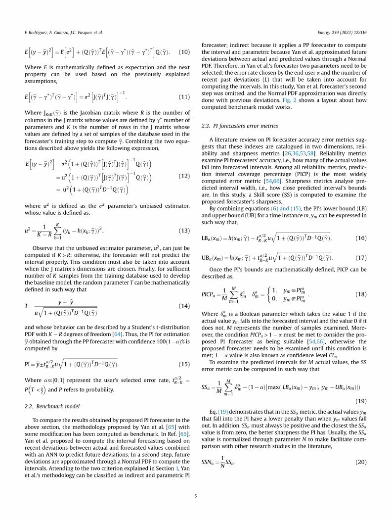
Fig. 3. Forecasted intervals and actual solar irradiation evolution for April 8, 2017(sunny day, PICP0:05 ¼ 100 and SSN0:05 ¼ 0:69).

F. Rodríguez, A. Galarza, J.C. Vasquez et al. Energy 239 (2022) 122116

Table 3 shows the SSN0.05 error metrics results for sunny, partiallycloudy and cloudy days. In addition, it must be taken into accountthat the N value for normalizing the SSN0:05 value is computed asthe average of solar irradiation per day per year, 158.02 W/m2. Forthose days that satisfied the condition PICPa > ð1 � aÞ, SSN, sSSN,SSNMAX and SSNMIN indicate the mean average, the standard de-viation and the maximum and minimum values. M ¼ 144 repre-sents the number of predicted values during each day.

After examining the results of Table 2, it is concluded that thelower the K parameter is, the higher the SSN0:05 index. Therefore, ifresults of sunny, partially cloudy and cloudy days are simulta-neously examined, it can be observed that there is a relationshipbetween interval width and forecasters accuracy, and thus thereliability (PICP0:05) and sharpness (SSN0:05) indexes must bebalanced. Although in this study we have chosen K ¼ 5937, thisparameter, as well as a error metric, can be modified by the enduser. Figs. 3e5 show the forecasted solar irradiation intervals for a

7

sunny, partially cloudy and cloud day, respectively.

3.2. Results of computed solar irradiation PI benchmark forecaster

As explained above, in computed benchmark two parametersneed to be selected: the error rate chosen by the end user a and thenumber of recent past deviations L that will be taken into accountfor computing the intervals. Predictions in the above section weredone with a ¼ 0:05 so, this value will be the same to ensure aproper comparison between both methods. Therefore, L is the onlyparameter that must be selected. For this purpose, a sensitivityanalysis was run, where in order to consider the computedbenchmark acceptable, parameter L is varied until the conditionPICPa > ð1�aÞ is met. Same criteria followed in above section toconstruct Tables 2 and 3 has been used to construct Tables 4 and 5that summarizes the results of the benchmark model.

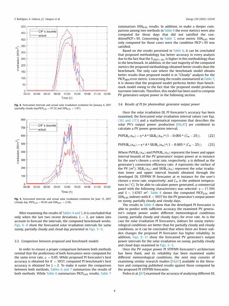
Fig. 4. Forecasted intervals and actual solar irradiation evolution for January 4, 2017(partially cloudy day,PICP0:05 ¼ 97:22 and SSN0:05 ¼ 1:07).

Fig. 5. Forecasted intervals and actual solar irradiation evolution for June 15, 2017(cloudy day, PICP0:05 ¼ 95:83 and SSN0:05 ¼ 2:56).

F. Rodríguez, A. Galarza, J.C. Vasquez et al. Energy 239 (2022) 122116

After examining the results of Tables 4 and 5, it is concluded thatonly when the last two recent deviations, L ¼ 2, are taken intoaccount to forecast the intervals, the computed benchmark works.Figs. 6e8 show the forecasted solar irradiation intervals for samesunny, partially cloudy and cloud day presented in Figs. 3e5.

3.3. Comparison between proposed and benchmark models

In order to ensure a proper comparison between both methodsremind that the predictions of both forecasters were computed forthe same error rate, a ¼ 0:05. While proposed PI forecaster's bestaccuracy is obtained for K ¼ 5937, computed PI benchmark's bestaccuracy is obtained for L ¼ 2: To make it easier the comparisonbetween both methods, Tables 6 and 7 summarizes the results ofboth methods. While Table 6 summarizes PICP0:05 results, Table 7

8

summarizes SSN0:05 results. In addition, to make a deeper com-parison among two methods in Table 6 the error metrics were alsocomputed for those days that did not satisfied the con-ditionPICP>95. Concerning to Table 7, error metric SSN0:05 wasonly computed for those cases were the condition PICP>95 wassatisfied.

Based on the results presented in Table 6, it can be concludedthat proposed methodology has better accuracy in every analysisdue to the fact that the %ðPICP>95Þ is higher in thismethodology thanin the benchmark. In addition, in the vast majority of the computedmetrics the proposed methodology obtained better results than thebenchmark. The only case where the benchmark model obtainsbetter results than proposed model is in “Cloudy” analysis for thePICPMIN error metric. Concerning the results summarized in Table 7,it is shown that the proposed model performs better than bench-mark model owing to the fact that the proposed model producesnarrower intervals. Therefore, this model has been used to computePV generators output power in the following section.

3.4. Results of PI for photovoltaic generator output power

Once the solar irradiation DL PI forecaster's accuracy has beenexamined, the forecasted solar irradiation interval values (see Eqs.(16) and (17)) and a mathematical expression that describes thesolar PV's output power production [36,47] are combined tocalculate a PV power generation interval,

PVPLBaðxmÞ¼ h *A * SILBaðxmÞ*ð1�0:005 * ðCm �25ÞÞ: (22)

PVPUBaðxmÞ¼ h *A * SIUBaðxmÞ*ð1�0:005 * ðCm �25ÞÞ: (23)

Where PVPLBaðxmÞ and PVPUBaðxmÞ represent the lower and upperinterval bounds of the PV generators' output power at m instancefor the user's chosen a error rate, respectively; h is defined as thegenerator's conversion efficiency rate; A represents the surface ofthe PV (m2); SILBaðxmÞ and SIUBaðxmÞ represent the solar irradia-tion lower and upper interval bounds obtained through thedeveloped DL STFFNN PI forecaster at m instance for the user'schosen a error rate, respectively; and Cm is the ambient tempera-ture in (�C). To be able to calculate power generated, a commercialpanel with the following characteristics was selected: h ¼ 17:59%and S ¼ 1:6767 m2. Table 8 shows the computed PICP0:05 andSSN0:05 indexes with K ¼ 5937 for the PV generator's output poweron sunny, partially cloudy and cloudy days.

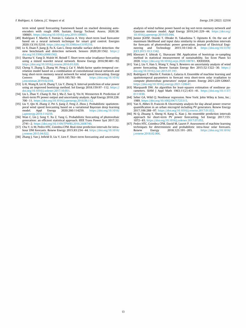
The results in Table 8 show that the developed PI forecaster isable to predict with sufficient accuracy the examined PV genera-tor's output power under different meteorological conditions(sunny, partially cloudy and cloudy days) for error rate. As is thecase for solar irradiation PI forecasters, indexes for sunny meteo-rological conditions are better than for partially cloudy and cloudyconditions, so it can be concluded that when there are fewer sud-den changes the proposed PI forecaster has higher reliability. Inaddition, Figs. 9e11 show the forecasted PV generator's outputpower intervals for the solar irradiation on sunny, partially cloudyand cloud days examined in Figs. 3e5.

Once the PV output power PI STFFNN forecaster's architecturehas been fixed, and its reliability has been examined underdifferent meteorological conditions, the next step consists ofexamining similar research studies [54,67] available in the litera-ture and comparing published results against those computed bythe proposed PI STFFNN forecaster.

Pedro et al. [67] examined the accuracy of analysing different DL

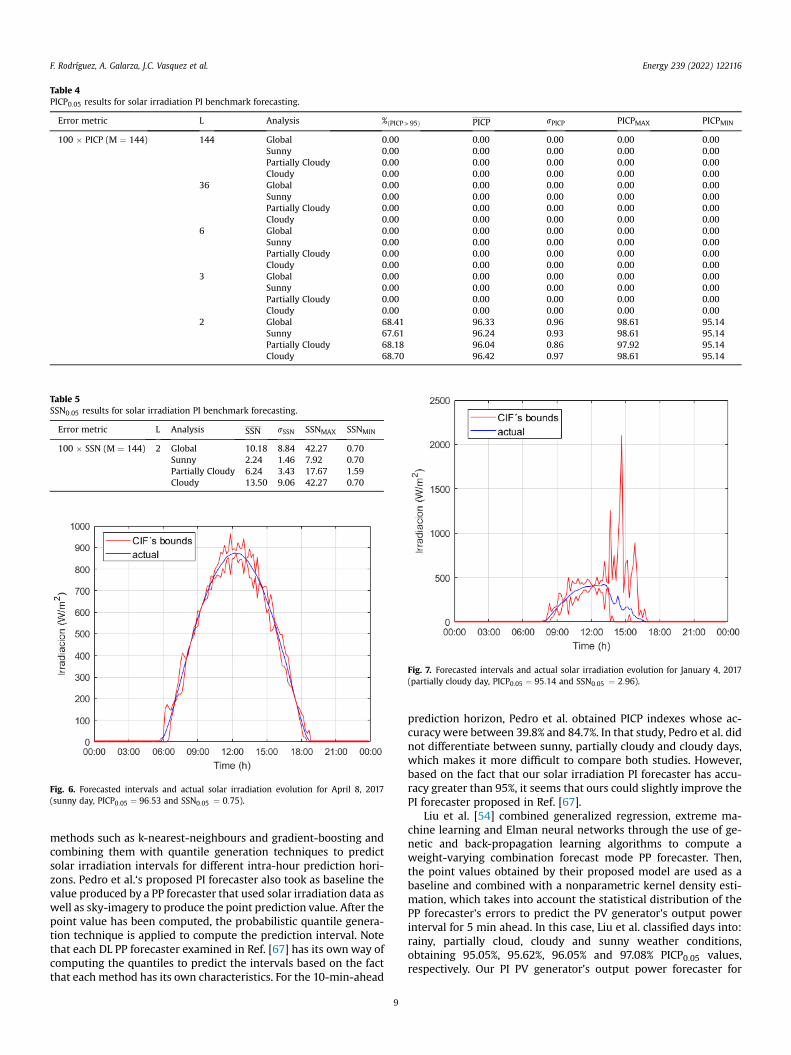
Table 4PICP0:05 results for solar irradiation PI benchmark forecasting.

Error metric L Analysis %ðPICP>95Þ PICP sPICP PICPMAX PICPMIN

100 � PICP (M ¼ 144) 144 Global 0.00 0.00 0.00 0.00 0.00Sunny 0.00 0.00 0.00 0.00 0.00Partially Cloudy 0.00 0.00 0.00 0.00 0.00Cloudy 0.00 0.00 0.00 0.00 0.00

36 Global 0.00 0.00 0.00 0.00 0.00Sunny 0.00 0.00 0.00 0.00 0.00Partially Cloudy 0.00 0.00 0.00 0.00 0.00Cloudy 0.00 0.00 0.00 0.00 0.00

6 Global 0.00 0.00 0.00 0.00 0.00Sunny 0.00 0.00 0.00 0.00 0.00Partially Cloudy 0.00 0.00 0.00 0.00 0.00Cloudy 0.00 0.00 0.00 0.00 0.00

3 Global 0.00 0.00 0.00 0.00 0.00Sunny 0.00 0.00 0.00 0.00 0.00Partially Cloudy 0.00 0.00 0.00 0.00 0.00Cloudy 0.00 0.00 0.00 0.00 0.00

2 Global 68.41 96.33 0.96 98.61 95.14Sunny 67.61 96.24 0.93 98.61 95.14Partially Cloudy 68.18 96.04 0.86 97.92 95.14Cloudy 68.70 96.42 0.97 98.61 95.14

Table 5SSN0:05 results for solar irradiation PI benchmark forecasting.

Error metric L Analysis SSN sSSN SSNMAX SSNMIN

100 � SSN (M ¼ 144) 2 Global 10.18 8.84 42.27 0.70Sunny 2.24 1.46 7.92 0.70Partially Cloudy 6.24 3.43 17.67 1.59Cloudy 13.50 9.06 42.27 0.70

Fig. 6. Forecasted intervals and actual solar irradiation evolution for April 8, 2017(sunny day, PICP0:05 ¼ 96:53 and SSN0:05 ¼ 0:75).

Fig. 7. Forecasted intervals and actual solar irradiation evolution for January 4, 2017(partially cloudy day, PICP0:05 ¼ 95:14 and SSN0:05 ¼ 2:96).

F. Rodríguez, A. Galarza, J.C. Vasquez et al. Energy 239 (2022) 122116

methods such as k-nearest-neighbours and gradient-boosting andcombining them with quantile generation techniques to predictsolar irradiation intervals for different intra-hour prediction hori-zons. Pedro et al.‘s proposed PI forecaster also took as baseline thevalue produced by a PP forecaster that used solar irradiation data aswell as sky-imagery to produce the point prediction value. After thepoint value has been computed, the probabilistic quantile genera-tion technique is applied to compute the prediction interval. Notethat each DL PP forecaster examined in Ref. [67] has its own way ofcomputing the quantiles to predict the intervals based on the factthat each method has its own characteristics. For the 10-min-ahead

9

prediction horizon, Pedro et al. obtained PICP indexes whose ac-curacywere between 39.8% and 84.7%. In that study, Pedro et al. didnot differentiate between sunny, partially cloudy and cloudy days,which makes it more difficult to compare both studies. However,based on the fact that our solar irradiation PI forecaster has accu-racy greater than 95%, it seems that ours could slightly improve thePI forecaster proposed in Ref. [67].

Liu et al. [54] combined generalized regression, extreme ma-chine learning and Elman neural networks through the use of ge-netic and back-propagation learning algorithms to compute aweight-varying combination forecast mode PP forecaster. Then,the point values obtained by their proposed model are used as abaseline and combined with a nonparametric kernel density esti-mation, which takes into account the statistical distribution of thePP forecaster's errors to predict the PV generator's output powerinterval for 5 min ahead. In this case, Liu et al. classified days into:rainy, partially cloud, cloudy and sunny weather conditions,obtaining 95.05%, 95.62%, 96.05% and 97.08% PICP0:05 values,respectively. Our PI PV generator's output power forecaster for

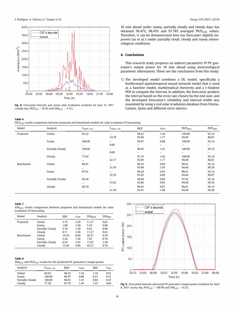
Fig. 8. Forecasted intervals and actual solar irradiation evolution for June 15, 2017(cloudy day, PICP0:05 ¼ 95:83 and SSN0:05 ¼ 4:15).

Table 6PICP0:05 results comparison between proposed and benchmark models for solar irradiat

Model Analysis %ðPICP>95Þ %ðPICP<95

Proposed Global 85.22 e

e 14.78

Sunny 100.00 e

e 0.00

Partially Cloudy 100.00 e

e 0.00

Cloudy 77.83 e

e 22.17

Benchmark Global 68.41 e

e 31.59

Sunny 67.61 e

e 32.39

Partially Cloudy 68.18 e

e 31.82

Cloudy 68.70 e

e 31.30

Table 7SSN0:05 results comparison between proposed and benchmark models for solarirradiation PI forecasting.

Model Analysis SSN sSSN SSNMAX SSNMIN

Proposed Global 3.74 2.50 11.27 0.63Sunny 1.88 1.04 5.10 0.66Partially Cloudy 2.74 1.58 6.92 0.98Cloudy 4.71 2.58 11.27 0.63

Benchmark Global 10.18 8.84 42.27 0.70Sunny 2.24 1.46 7.92 0.70Partially Cloudy 6.24 3.43 17.67 1.59Cloudy 13.50 9.06 42.27 0.70

Table 8SSN0:05 and PICP0:05 results for the predicted PV generator's output power.

Analysis %ðPICP>95Þ PICP sPICP SSN sSSN

Global 84.93 98.25 1.54 1.16 0.81Sunny 100.00 99.47 0.88 0.57 0.31Partially Cloudy 100.00 98.45 1.41 0.84 0.47Cloudy 77.39 97.78 1.45 1.47 0.85

F. Rodríguez, A. Galarza, J.C. Vasquez et al. Energy 239 (2022) 122116

10

10 min ahead under sunny, partially cloudy and cloudy days hasobtained 99.47%, 98.45% and 97.78% averaged PICP0:05 values.Therefore, it can be demonstrated how our forecaster slightly im-proves Liu et al.‘s under partially cloud, cloudy and sunny meteo-rological conditions.

4. Conclusions

This research study proposes an indirect parametric PI PV gen-erator's output power for 10 min ahead using meteorologicalparameter information. These are the conclusions from this study:

1) The developed model combines a DL model, specifically afeedforward spatiotemporal neural network model that is usedas a baseline model, mathematical theorems and a t-StudentPDF to compute the interval. In addition, the forecaster predictsthe interval based on the error rate chosen by the end user, andthe developed forecaster's reliability and interval width wasexamined by using a real solar irradiation database fromVitoria-Gasteiz, Spain and different error metrics.

ion PI forecasting.

Þ PICP sPICP PICPMAX PICPMIN

98.25 1.54 100.00 95.1492.06 1.77 94.44 86.81

99.47 0.88 100.00 95.14e e e e

98.45 1.41 100.00 95.14e e e e

97.79 1.45 100.00 95.1492.09 1.77 94.44 86.81

96.33 0.96 98.61 95.1493.48 1.03 94.44 90.28

96.24 0.93 98.61 95.1493.45 0.89 94.44 90.97

96.04 0.86 97.92 95.1493.86 0.85 94.44 90.36

96.42 0.97 98.61 95.1493.41 1.08 94.44 90.28

Fig. 9. Forecasted intervals and actual PV generator's output power evolution for April8, 2017 (sunny day, PICP0:05 ¼ 100:00 and SSN0:05 ¼ 0:23).

Fig. 10. Forecasted intervals and actual PV generator's output power evolution forJanuary 4, 2017 (partially cloudy day, PICP0:05 ¼ 97:22 and SSN0:05 ¼ 0:35).

Fig. 11. Forecasted intervals and actual PV generator's output power evolution for June15, 2017 (cloudy day, PICP0:05 ¼ 95:14 and SSN0:05 ¼ 0:78).

F. Rodríguez, A. Galarza, J.C. Vasquez et al. Energy 239 (2022) 122116

2) The solar irradiation PI forecaster has been validated with theentire data of 2017. Attending to the accuracy results shown inTable 6, proposed forecaster satisfied required condition ofPICP0:05 >0:95 in the 85.22% days of 2017. While for those dayswhich met the condition PICP0:05 is 98.25, the PICP0:05 value forthose days that did notmeet the condition is 92.06. If these errormetrics results are contrasted against those provided bycomputed benchmark, only the 68.41% of the days of 2017 metthe condition of PICP0:05 >0:95. While for those days which metthe condition PICP0:05 is 96.33, the PICP0:05 value for those daysthat did not meet the condition is 93.48. Therefore, it wasdemonstrated that proposed forecaster performs better thancomputed benchmark PI forecaster. The reason why PICP0:05values is higher in the benchmark model than in proposed onefor those days that did not meet the condition, relies on the factthat is that there were some days close to meet the condition.

11

Therefore, the value of the PICP0:05 error metric rises up in thebenchmark model.

3) Attending to the sharpness error metrics results shown inTable 7, for those days where the condition PICP0:05 >0:95 wasmet, proposed prediction model obtained a SSN0:05 error metricof 3.74, whereas computed benchmark model got 10.18. Thiserror metric was computed for each subset data of sunny,partially cloudy and cloudy days; while the obtained SSN0:05 forproposed model is 1.88, 2.74 and 4.71, respectively, forcomputed benchmark is 2.24, 6.24 and 13.50. Therefore, it isconcluded that proposed forecaster does not only have higheraccuracy, but also produces narrower intervals.

4) Through the predictions done by proposed solar irradiation PIforecaster, PV output power generator's intervals werecomputed. For entire 2017 year's data, the 84.93% of computeddays satisfied the condition PICP0:05 >0:95, with a global PICP of98.25 and SSN of 1.16. If each type of days subsets are examinedsunny and partially cloudy days obtained remarkable results sueto the fact that in both cases the 100.00% of computed dayssatisfied the condition PICP0:05 >0:95, this value reduces to the77.39% in cloudy days. PICP and SSN error metrics werecomputed for each subset data of sunny, partially cloudy andcloudy days; while the obtained PICP for proposed model are99.47, 98.45 and 97.78, respectively, for SSNare 0.57, 0.84 and1.47. Therefore, developed forecaster makes it possible to pro-vide further information to power systems' decision makers,doing possible in near future not only to provide power gener-ation but also ancillary services, maximizing PV generators'profits

5) The computed numerical results of this research activity and thesensitivity analyses were done using meteorological data fromthe location of Vitoria-Gasteiz, Spain. While the database for theyears 2015e16 was applied for computing JðbgÞ, the 2017 data-base was applied to calculate QðbgÞ. Therefore, the examinedmathematical methodology for PV generator output power PIforecasting can be easily applied in other locations. However,the biggest disadvantage of the presentmethodology is the needto have a database from the target station to fit the model'sparameters.

Credit author statement

Fermín Rodríguez: Conceptualization, Methodology, Validation,Resources, Investigation, Writing e original draft, Ainhoa Galarza:Methodology, Software, Resources, Investigation, Writing-Reviewing and Editing. Juan C. Vasquez: Formal analysis, Supervi-sion, Writing- Reviewing and Editing. Josep M. Guerrero: Concep-tualization, Visualization, Writing- Reviewing and Editing

Declaration of competing interest

The authors declare that they have no known competingfinancial interests or personal relationships that could haveappeared to influence the work reported in this paper.

Acknowledgements

The authors would like to thank the Basque Government'sDepartment of Education for financial support through theResearcher Formation Programme; grant numberPRE_2020_2_0038.

The authors would like to thank Fundaci�on Caja Navarra, Obra

F. Rodríguez, A. Galarza, J.C. Vasquez et al. Energy 239 (2022) 122116

Social La Caixa and University of Navarra for financial supportthrough the Mobility Research Formation Programme; grantnumber MOVIL-2019-25.

J. M. Guerrero was supported by VILLUM FONDEN under theVILLUM Investigator Grant (no. 25920): Center for Research onMicrogrids (CROM); www.crom.et.aau.dk.

References

[1] Li J, Lan F, Wei H. A scenario optimal reduction method for wind power timeseries. IEEE Trans Power Syst 2016;32:1657e8. https://doi.org/10.1109/TPWRS.2015.2412687.

[2] Wüstenhagen R, Bilharz M. Green energy market development in Germany:effective public policy and emerging customer demand. Energy Pol 2006;34:1681e96. https://doi.org/10.1016/j.enpol.2004.07.013.

[3] El-Baz W, Tzscheutschler P, Wagner U. Day-ahead probabilistic PV generationforecast for buildings energy management systems. Sol Energy 2018;171:478e90. https://doi.org/10.1016/j.solener.2018.06.100.

[4] BP. BP energy outlook 2019. 2019. https://www.bp.com/content/dam/bp/business-sites/en/global/corporate/pdfs/energy-economics/energy-outlook/bp-energy-outlook-2019.pdf. [Accessed 4 March 2020].

[5] REN21. Renewables 2019 global satuts report. 2019. https://www.ren21.net/wp-content/uploads/2019/05/gsr_2019_full_report_en.pdf. [Accessed 4March 2020].

[6] Pillot B, Muselli M, Poggi P, Dias JB. Historical trends in global energy policyand renewable power system issues in Sub-Saharan Africa: the case of solarPV. Energy Pol 2019;127:113e24. https://doi.org/10.1016/j.enpol.2018.11.049.

[7] Maron H, Klemisch H, Maron B. Marktakteure erneuerbare Energie-Anlagen inder Stromerzeugung. 2011. p. 1e92. https://sverigesradio.se/diverse/appdata/isidor/files/3345/12617.pdf. [Accessed 26 July 2020].

[8] Liu J, Fang W, Zhang X, Yang C. An improved photovoltaic power forecastingmodel with the assistance of aerosol index data. IEEE Transaction on Sus-tainable Energy 2015;6:434e42. https://doi.org/10.1109/TSTE.2014.2381224.

[9] Li Y, He Y, Su Y, Shu L. Forecasting the daily power output of a grid-connectedphotovoltaic system based on multivariate adaptive regression splines. ApplEnergy 2016;180. https://doi.org/10.1016/j.apenergy.2016.07.052. 392e40.

[10] Ferlito S, Adinolfi G, Graditi G. Comparative analysis of data-driven methodsonline and offline trained to the forecasting of grid-connected photovoltaicplant production. Appl Energy 2017;205:116e29. https://doi.org/10.1016/j.apenergy.2017.07.124.

[11] Wang Y, Zhang N, Kang C, Miao M, Shi R, Xia Q. An efficient approach to powersystem uncertainty analysis with high-dimensional dependencies. IEEE TransPower Syst 2017;33:2984e94. https://doi.org/10.1109/TPWRS.2017.2755698.

[12] Sahoo AK, Sahoo SK. Energy forecasting for grid connected MW range solar PVsystem. In: 7th India International conference on power electronics (IICPE);2016. https://doi.org/10.1109/IICPE.2016.8079388.

[13] Yin L, Yu T, Zhang X, Yang B. Relaxed deep learning for real-time economicgeneration dispatch and control with unified time scale. Energy 2018;149:11e23. https://doi.org/10.1016/j.energy.2018.01.165.

[14] Majumder I, Behera MK, Nayak N. Solar power forecasting using a hybridEMD-ELM method. In: International conference on circuits power andcomputing technologies (ICCPCT); 2017. https://doi.org/10.1109/ICCPCT.2017.8074179.

[15] Frías-Paredes L, Mallor F, Gast�on-Romeo M, Le�on T. Assessing energy fore-casting inaccuracy by simultaneously considering temporal and absolute er-rors. Energy Convers Manag 2017;142:533e46. https://doi.org/10.1016/j.enconman.2017.03. 056.

[16] Ahmed R, Sreeram V, Mishra Y, Arif MD. A review and evaluation of the state-of-the-art in PV solar power forecasting: techniques and optimization. RenewSustain Energy Rev 2020;124:109792. https://doi.org/10.1016/j.rser.2020.109792.

[17] Zhang J, Verschae R, Nobuhara S, Lalonde JF. Deep photovoltaic nowcasting.Sol Energy 2018;176:267e76. https://doi.org/10.1016/j.solener.2018.10.024.

[18] Chen X, Du Y, Lim E, Wen H, Jiang L. Sensor network based PV power now-casting with spatio-temporal preselection for grid-friendly control. Appl En-ergy 2019;255:113760. https://doi.org/10.1016/j.apenergy.2019.113760.

[19] Chu Y, Li M, Coimbra CFM. Sun-tracking imaging system for intra-hour DNIforecasts. Renew Energy 2016;96:792e9. https://doi.org/10.1016/j.renene.2016.05.041.

[20] Jamal T, Carter C, Schmidt T, Shafiullah GM, Calais M, Urmee T. An energy flowsimulation tool for incorporating short-term PV forecasting in a diesel-PV-battery off-grid power supply system. Appl Energy 2019;254:113718.https://doi.org/10.1016/j.apenergy.2019.113718.

[21] Amanpreet K, Nonnenmacher L, Pedro HTC, Coimbra CFM. Benefits of solarforecasting for energy imbalance markets. Renew Energy 2016;86:819e30.https://doi.org/10.1016/j.renene.2015.09.011.

[22] David M, Luis MA, Lauret P. Comparison of intraday probabilistic forecastingof solar irradiance using only endogenous data. Int J Forecast 2018;34:529e47. https://doi.org/10.1016/j.ijforecast.2018.02.003.

[23] Pedro HTC, Coimbra CFM. Assessment of forecasting techniques for solarpower production with no exogenous inputs. Sol Energy 2012;86:2017e28.

12

https://doi.org/10.1016/j.solener.2012.04.004.[24] Sperati S, Alessandrini S, Monache LD. An application of the ECMWF Ensemble

Prediction System for short-term solar power forecasting. Sol Energy2016;113:437e50. https://doi.org/10.1016/j.solener.2016.04.016.

[25] Araya IA, Valle C, Allende H. A Multi-Scale Model based on the Long Short-Term Memory for day ahead hourly wind speed forecasting. Pattern RecognLett 2019. https://doi.org/10.1016/j.patrec.2019.10.011.

[26] Verbois H, Rusydi A, Thiery A. Probabilistic forecasting of day-ahead solarirradiance using quantile gradient boosting. Sol Energy 2018;173:313e27.https://doi.org/10.1016/j.solener.2018.07.071.

[27] Gürter M, Paulsen T. The effect of wind and solar power forecasts on day-ahead and intraday electricity prices in Germany. Energy Econ 2018;75:150e62. https://doi.org/10.1016/j.eneco.2018.07.006.

[28] Chazarra M, P�erez-Díaz JI, García-Gonz�alez J, Helseth A. Economic effects offorecasting inaccuracies in the automatic frequency restoration service for theday-ahead energy and reserve scheduling of pumped storage plants. ElecPower Syst Res 2019;174:105850. https://doi.org/10.1016/j.epsr.2019.04.028.

[29] Elsinga B, van Sark WGJHM. Short-term peer-to-peer solar forecasting in anetwork of photovoltaic systems. Appl Energy 2017;206:1464e83. https://doi.org/10.1016/j.apenergy.2017.09.115.

[30] Lorenz E, Heineman D. Prediction of solar irradiance and photovoltaic power.Compreh Renewable Energy 2012;1:239e92. https://doi.org/10.1016/B978-0-08-087872-0.00114-1.

[31] Diagne M, David M, Lauret P, Boland J, Schmutz N. Review of solar irradianceforecasting methods and a proposition for small-scale insular grids. RenewSustain Energy Rev 2013;27:65e76. https://doi.org/10.1016/j.rser.2013.06.042.

[32] European Union and International Renewable Energy Agency (IRENA).Renewable energy Prospects for the European union. 2018. https://www.irena.org/-/media/Files/IRENA/Agency/Publication/2018/Feb/IRENA_REmap_EU_2018.pdf. [Accessed 15 July 2020].

[33] International Renewable Energy Agency (IRENA). https://www.irena.org/-/media/Files/IRENA/Agency/Publication/2019/Feb/IRENA_Innovative_ancillary_services_2019.pdf?la¼en&hash¼F3D83E86922DEED7AA3DE3091F3E49460C9EC1A0. [Accessed 16 July 2020].

[34] Banshwar A, Sharma NK, Sood YR, eta al. Renewable energy sources as a newparticipant in ancillary service markets. Energy Strategy Reviews 2017;18:106e20. https://doi.org/10.1016/j.esr.2017.09.009.

[35] Ayvazo�gluyüksel €O, Filik ÜB. Estimation methods of global solar irradiation,cell temperature and solar power forecasting: a review and a case study inEskisehir. Renew Sustain Energy Rev 2018;91:639e53. https://doi.org/10.1016/j.rser.2018.03.084.

[36] Rodríguez F, Bazmohammadi N, Guerrero JM, Galarza A. A very short-termprobabilistic prediction interval forecaster for reducing load uncertaintylevel in smart grids. Appl Sci 2021;11(6):2538. https://doi.org/10.3390/app11062538.

[37] Rodríguez F, Genn M, Font�an L, Galarza A. Very short-term temperatureforecaster using MLP and N-nearest stations for calculating key control pa-rameters in solar photovoltaic generation. Sustainable Energy Technologiesand Assessments 2021;45:101085. https://doi.org/10.1016/j.seta.2021.101085.

[38] Rodríguez F, Florez-Tapia AM, Font�an L, Galarza A. Very short-term windpower density forecasting trough artificial neural networks for microgridcontrol. Renew Energy 2020;145:1517e27. https://doi.org/10.1016/j.renene.2019.07.067.

[39] Dupr�e A, Dobrinski P, Alnzo B, Bados J, Briad C, Plougoven R. Sub-hourlyforecasting of wind speed and wind energy. Renew Energy 2020:2373e9.https://doi.org/10.1016/j.renene.2019.07.161.

[40] Wang GC, Urquhart B, Kleissl J. Cloud base height estimates from sky imageryand a network of pyranometers. Sol Energy 2019;184:594e609. https://doi.org/10.1016/j.solener.2019.03.101.

[41] Polo J. Solar global horizontal and direct normal irradiation maps in Spainderived from geostationary satellites. J Atmos Sol Terr Phys 2015;130e131:81e8. https://doi.org/10.1016/j.jastp.2015.05.015.

[42] Agoua XG, Girard R, Kariniotakis G. Short-term spatio-temporal forecasting ofphotovoltaic power production. IEEE Transactions on Sustainable Energy2018;9:538e46. https://doi.org/10.1109/TSTE.2017.2747765.

[43] Tang N, Mao S, Wang Y, Nelms RM. Solar power generation forecasting with aLASSO- based approach. IEEE Internet of Things Journal 2018;5:2933e44.https://doi.org/10.1109/JIOT.2018.2877510.

[44] Prado F, Minutolo MC, Kristjanpoller W. Forecasting based on an ensembleautoregressive moving average - adaptive neuro - fuzzy inference system eneural network - genetic algorithm framework. Energy 2020;197:117159.https://doi.org/10.1016/j.energy.2020.117159.

[45] David M, Ramahatana F, Trombe PJ, Lauret P. Probabilistic forecasting of thesolar irradiance with recursive ARMA and GARCH models. Sol Energy2016;133:55e72. https://doi.org/10.1016/j.solener.2016.03.064.

[46] Singh ASN, Mohapatra A. Repeated wavelet transform based ARIMA model forvery short-term wind speed forecasting. Renew Energy 2019;136:758e68.https://doi.org/10.1016/j.renene.2019.01.031.

[47] Rodríguez F, Fleetwood A, Galarza A, Font�an F. Predicting solar energy gen-eration through artificial neural networks using weather forecasts formicrogrid control. Renew Energy 2018;126:855e64. https://doi.org/10.1016/j.renene.2018.03.070.

[48] Jahangir H, Golkar MA, Alhameli F, Mazouz A, Ahmadian A, Elkamel A. Short-

F. Rodríguez, A. Galarza, J.C. Vasquez et al. Energy 239 (2022) 122116

term wind speed forecasting framework based on stacked denoising auto-encoders with rough ANN. Sustain. Energy Technol. Assess. 2020;38:100601. https://doi.org/10.1016/j.seta.2019.100601.

[49] Rodríguez F, Martín F, Font�an L, Galarza A. Very short-term load forecasterbased on a neural network technique for smart grid control. Energies2020;13(19):5210. https://doi.org/10.3390/en13195210.

[50] Lv X, Duan F, Jiang JJ, Fu X, Gan L. Deep metallic surface defect detection: thenew benchmark and detection network. Sensors 2020;20:1562. https://doi.org/10.3390/s20061562.

[51] Sharma V, Yang D, Walsh W, Reindl T. Short term solar irradiance forecastingusing a mixed wavelet neural network. Renew Energy 2016;90:481e92.https://doi.org/10.1016/j.renene.2016.01.020.

[52] Cheng Y, Zhang S, Zhang W, Peng J, Cai Y. Multi-factor spatio-temporal cor-relation model based on a combination of convolutional neural network andlong short-term memory neural network for wind speed forecasting. EnergyConvers Manag 2019;185:783e99. https://doi.org/10.1016/j.enconman.2019.02.018.

[53] Li K, Wang R, Lei H, Zhang T, Liu Y, Zheng X. Interval prediction of solar powerusing an improved bootstrap method. Sol Energy 2018;159:97e112. https://doi.org/10.1016/j.solener.2017.10.051.

[54] Liu L, Zhao Y, Chang D, Xie J, Ma Z, Sun Q, Yin H, Wennerten R. Prediction ofshort-term PV power output and uncertainty analysis. Appl Energy 2018;228:700e11. https://doi.org/10.1016/j.apenergy.2018.06.112.

[55] Liu Y, Qin H, Zhang Z, Pei S, Jiang Z, Feng Z, Zhou J. Probabilistic spatiotem-poral wind speed forecasting based on a variational Bayesian deep learningmodel. Appl Energy 2020;260:114259. https://doi.org/10.1016/j.apenergy.2019.114259.

[56] Wan C, Lin J, Song Y, Xu Z, Yang G. Probabilistic forecasting of photovoltaicgeneration: an efficient statistical approach. IEEE Trans Power Syst 2017;32:2741e2. https://doi.org/10.1109/TPWRS.2016.2608740.

[57] Chu Y, Li M, Pedro HTC, Coimbra CFM. Real-time prediction intervals for intra-hour DNI forecasts. Renew Energy 2015;83:234e44. https://doi.org/10.1016/j.renene.2015.04.022.

[58] Zhang J, Yan J, Infield D, Liu Y, Lien F. Short-term forecasting and uncertainty

13

analysis of wind turbine power based on log sort-term memory network andGaussian mixture model. Appl Energy 2019;241:229e44. https://doi.org/10.1016/j.apenergy.2019.03.044.

[59] Junior JGDSF, Oozeki T, Ohtake H, Takashima T, Ogimoto K. On the use ofmaximum likelihood and input data similarity to obtain prediction intervalsfor forecasts of photovoltaic power generation. Journal of Electrical Engi-neering and Technology 2015;10:1342e8. https://doi.org/10.5370/JEET.2015.10.3.1342.

[60] Khosravi F, Izbirak G, Shavarani SM. Application of bootstrap re-samplingmethod in statistical measurement of sustainability. Soc Econ Plann Sci2020. https://doi.org/10.1016/j.seps.2020.100781. XXXXXXX.

[61] Yan J, Liu Y, Han S, Wang Y, Feng S. Rewievs on uncertainty analysis of windpower forecasting. Renew Sustain Energy Rev 2015;52:1322e30. https://doi.org/10.1016/j.rser.2015.07.197.

[62] Rodríguez F, Martín F, Font�an L, Galarza A. Ensemble of machine learning andspatiotemporal parameters to forecast very short-term solar irradiation tocompute photovoltaic generators' output power. Energy 2021;229:120647.https://doi.org/10.1016/j.energy.2021.120647.

[63] Marquardt DW. An algorithm for least-squares estimation of nonlinear pa-rameters. SIAM J Appl Math 1963;11(2):431e41. https://doi.org/10.1137/0111030.

[64] Seber GA, Wild CJ. Nonlinear regression. New York: John Wiley & Sons, Inc.;1989. https://doi.org/10.1002/0471725315.

[65] Yan X, Abbes D, Francois B. Uncertainty analysis for day ahead power reservequantification in an urban microgrid including PV generators. Renew Energy2017;106:288e97. https://doi.org/10.1016/j.renene.2017.01.022.

[66] Ni Q, Zhuang S, Sheng H, Kang G, Xiao J. An ensemble prediction intervalsapproach for short-term PV power forecasting. Sol Energy 2017;155:1072e83. https://doi.org/10.1016/j.solener.2017.07.052.

[67] Pedro HTC, Coimbra CFM, David M, Lauret P. Assessment of machine learningtechniques for deterministic and probabilistic intra-hour solar forecasts.Renew Energy 2018;123:191e203. https://doi.org/10.1016/j.renene.2018.02.006.