Using Combat Simulation and Sensitivity Analysis to ...mssanz.org.au/modsim2017/D1/chau.pdf · Using Combat Simulation and Sensitivity Analysis to Support Evaluation of Land Combat

Using Combat Simulation and Sensitivity Analysis to Support Evaluation of Land Combat Vehicle

Configurations

William Chau, Andrew Gill, and Dion Grieger

Joint and Operations Analysis Division, Defence Science and Technology Group Email: [email protected]

Abstract: Combat simulations can be used to compare the operational effectiveness of alternative system configurations in a well-defined military context via an experimental layout. However, modelling complex warfighting is challenging as there are many parameters in high-fidelity combat simulations that can affect the outcome, particularly those relating to the environment and the implementation of tactical decision making, and some of these can be quite uncertain. Exploring all possible parameter combinations is often infeasible; therefore a well-designed experiment is required to understand the impact on the performance rankings of alternative system configurations.

This paper describes a case study using the COMBATXXI closed-loop simulation to estimate the performance sensitivity of land combat vehicle configurations within a doctrinal scenario. In total, there were 22 configurations with different combinations of firepower, protection and other sub-system components that were required to be analysed. A multiple comparison procedure involving statistical tests was used to analyse the baseline scenario against a number of performance metrics. In order to isolate the effects of the sub-systems, regression analysis was used.

To improve the robustness of the baseline results, sensitivity analysis using a fractional factorial experimental design was applied to uncertain environmental, tactical and system parameters in the combat simulation. The case study results identified a subset of parameters that contribute to changes in the metrics and, in turn, the performance rankings of the configurations. A combination of environmental and tactical parameters was found to alter the performance rankings of configurations when compared to the baseline results.

The differences in the configurations performances and the effects of the components were subjected to both statistical and practical significance tests. These significances are important to interpreting the insights for military experts. Performing sensitivity analysis and justifying the model assumptions allowed for an increased understanding between the model parameters and the performance rankings of the land combat vehicle configurations. This approach can be used to reduce uncertainty in the analysis and provide additional confidence for military decision makers.

Keywords: Land combat, simulation, experimental design, sensitivity analysis

22nd International Congress on Modelling and Simulation, Hobart, Tasmania, Australia, 3 to 8 December 2017 mssanz.org.au/modsim2017

536

Chau, W., Gill, A.W. and Grieger, D., Using Combat Simulation and Sensitivity Analysis to Support Evaluation of Land Combat Vehicle Configurations

1. INTRODUCTION

High-fidelity combat simulations are often employed as part of a multi-method approach to compare the operational effectiveness of alternative combat systems or tactics described by Bowley et al. (2003). Modelling complex warfighting is complicated by the large number of parameters that can impact operational effectiveness. The stochasticity of these simulations and the presence of uncertain model parameters requires the sensitivity of model output metrics and the subsequent performance rankings of the alternatives systems to be analysed. Due to time and resource constraints of high-fidelity combat simulations; it is often challenging to effectively and efficiently explore all possible parameter combinations, therefore a well-crafted experimental design plays an important role as described by Cochran and Cox (1957). Common experimental designs include one-factor-at-a-time (OFAT) screening by Daniel (1973), fractional factorial designs by Box and Hunter (1961) and Latin hypercube sampling (LHS) by McKay et al. (1979). Previous work conducted by Feil (1991) applied sensitivity analysis (by incorporating an experimental design) on the JANUS combat simulation in order to investigate how changes to battle parameters affect the measure of performance.

This paper explores the use of sensitivity analysis and experimental design to analyse the differences in performance rankings and output metrics of alternative land combat vehicles. Sensitivity analysis provides a greater understanding of the impact of the uncertain combat simulation parameters and the subsequent robustness of the conclusions drawn. A good experimental design maximizes the parameter search space while minimising the overall number of replications required of the simulation. A case study using the Combined Arms Analysis Tool for the 21st Century (COMBATXXI) simulation developed by TRAC (2015) is used to highlight the methods and challenges associated with the analysis of these types of simulations.

2. BACKGROUND

COMBATXXI is a non-interactive, entity-level, high-fidelity combat simulation which can be used for the analysis of alternative systems, employment explorations or system sensitivities. The model is able to represent force-on-force scenarios (down to the individual soldier), system components of land combat vehicles (such as firepower and sensors), tactical decision making and environmental factors (such as terrain and light levels). In this case study, two alternative land combat vehicle options (Option A and B) were explored using COMBATXXI. Different configurations of firepower, protection, sensor and other sub-system options were considered for each option. A large set of Option A configurations and a smaller set of Option B configurations (see Figure 1) were chosen to test in a feasible force-on-force military scenario. For each of the configurations 200 replications were run in order to provide a sufficient output for the statistical analysis. Output metrics pertaining to lethality, vulnerability, knowledge and signature drawn from subject matter experts were used to measure the performance of each configuration (see Table 1).

Table 1. Description of Metrics

Metric Type Description Mission Success A Mission Success metric was used to identify if the configurations used in the scenario would achieve

a successful mission. A Blue Mission Success is determined by subject matter experts (SMEs) and can change depending on the type of scenario. An example of a Mission Success could be if the Blue force stopped the Red force from reaching the final report line.

Lethality Lethality metrics measure how lethal the implemented configuration is against the enemy force. Examples of Lethality metrics includes the number of Red vehicles catastrophically killed and the number of Red infantry killed.

Vulnerability Vulnerability metrics measure how vulnerable the implemented configuration is among their friendly force. Examples of Vulnerability metrics include the number of Blue vehicles catastrophically killed and the number of Blue infantry killed.

Knowledge Knowledge metrics measure how well the Blue Force knows about the Red Force. An example of Knowledge metric is the number of Red detections by Blue.

Signature Signature metrics measures how well the Red Force knows about the Blue Force. An example of Signature metric is the number of Blue detections by Red.

3. OVERVIEW OF ANALYSIS METHODS

In this section, we split the analysis methods in two parts. The first part describes the comparison of the baseline results of the case study using statistical tests and regression analysis. The second part describes a design of experiments approach to sensitivity analysis which was used to determine the robustness of the baseline results.

537


3.1 Comparison of Vehicle Configurations

The statistical tests and regression analysis used here complement each other to provide a strong understanding of the land combat vehicle and its sub-systems. The statistical methods test the hypothesis that the output metric values for each of the options are from the same distribution; this seeks to find differences between options. The regression analysis seeks to isolate the effects of the configuration components.

Statistical Ranking and Visualisation

Once a set of baseline results were obtained for all configurations, a comparison of their performance against each metric was made using a number of statistical tests. The configuration's statistical ranking value was obtained through the multiple comparison procedure based on the works of Kendall (1948) and Villacorta & Sáez (2015). In the first step, the Friedman (1937) omnibus non-parametric test was used to detect differences among groups; second, the Wilcoxon (1945) Signed Ranked test was used to rank the performance of each configuration against each metric1 by using pairwise comparisons. The Cochran (1950) and McNemar (1947) tests were used for binary metrics such as mission success. The pairwise comparisons consist of comparing a pair of configurations over the replications of the simulation of a particular metric. During the pairwise comparisons, a configuration’s score was increased by '+1' for statistically better outcomes, by '-1' for statistically worse outcomes or by '0' for being statistically the same. The accumulated score for the configurations were their statistical performance ranking value.

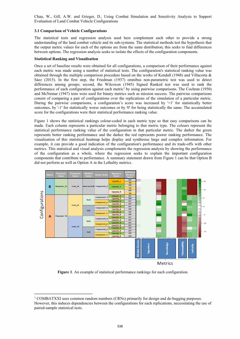
Figure 1 shows the statistical rankings colour-coded in each metric type so that easy comparisons can be made. Each column represents a particular metric belonging to that metric type. The colours represent the statistical performance ranking value of the configuration in that particular metric. The darker the green represents better ranking performance and the darker the red represents poorer ranking performance. The visualisation of this statistical heatmap helps display and synthesise large and complex information. For example, it can provide a good indication of the configuration's performance and its trade-offs with other metrics. This statistical and visual analysis complements the regression analysis by showing the performance of the configuration as a whole, where the regression seeks to explain the important configuration components that contribute to performance. A summary statement drawn from Figure 1 can be that Option B did not perform as well as Option A in the Lethality metrics.

Figure 1. An example of statistical performance rankings for each configuration.

1 COMBATXXI uses common random numbers (CRNs) primarily for design and de-bugging purposes. However, this induces dependencies between the configurations for each replications, necessitating the use of paired-sample statistical tests.

538


Regression The configurations for the combat vehicle options above represent full factorial designs over a small number of configuration components. For Option A each of four components had two level settings so the dth row of the design matrix ( , , , ) is one of the 2 = 16 possible combinations. The regression focused on estimating the main effect each configuration component has on each of the metrics in Table 1 (e.g. how much did protection contribute to the mission success of Blue?), as well as the effect, if any, of any two-way interactions between components (e.g. was there a combat multiplier effect between protection and mobility on the number of Blue infantry killed?). We approximated the study metric for each configuration (denoted by ) by an equation linear in these unknown main effects (denoted by ) and two-way interaction effects (denoted by β ):

≈ + ∑ + ∑ ∑ , = 1, … ,16 (1)

or ≈ where the model matrix = ( , , . . , , , … , , … , ) and is the j-th column of the design matrix . The Least Squares estimates of the effects are the solutions of the linear equations = which for a full factorial design simplifies to = (since the orthogonality of the

design ensures the inverse of exists and is diagonal).

For Option B, one component had two level settings but the other component had three level settings. Since this latter component was qualitative, the correct approach by Kleijnen (2007) was to use three two level factors – one for each level setting – and to include a constraint that only one of them may be at their ‘high’ level setting. So the dth row of the design matrix ( , , , ) was one of the 2 3 = 6 possible combinations of these two components, and represented one of the Option B configurations. However, this design did not allow an estimation of the two-way interactions between these two components (while tables of mixed level designs have existed for many years, e.g. Connor & Young (1961), these have been for 2 3 with + ≥ 5 which doesn’t apply here). The regression equation is therefore:

≈ + ∑ , ∑ = 1, = 1, … ,6; ∈ 0,1 (2)

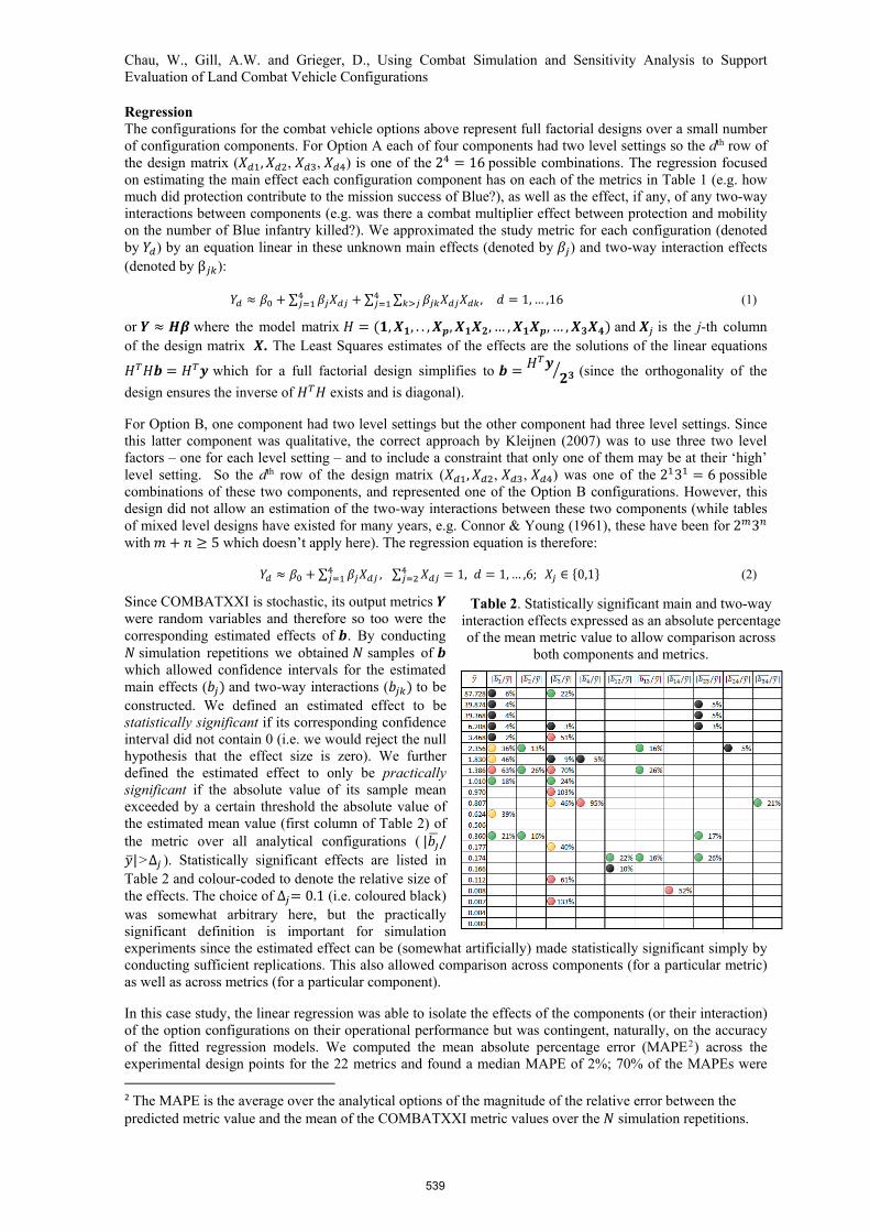
Since COMBATXXI is stochastic, its output metrics were random variables and therefore so too were the corresponding estimated effects of . By conducting simulation repetitions we obtained samples of which allowed confidence intervals for the estimated main effects ( ) and two-way interactions ( ) to be constructed. We defined an estimated effect to be statistically significant if its corresponding confidence interval did not contain 0 (i.e. we would reject the null hypothesis that the effect size is zero). We further defined the estimated effect to only be practically significant if the absolute value of its sample mean exceeded by a certain threshold the absolute value of the estimated mean value (first column of Table 2) of the metric over all analytical configurations ( | /|>∆ ). Statistically significant effects are listed in Table 2 and colour-coded to denote the relative size of the effects. The choice of ∆ = 0.1 (i.e. coloured black) was somewhat arbitrary here, but the practically significant definition is important for simulation experiments since the estimated effect can be (somewhat artificially) made statistically significant simply by conducting sufficient replications. This also allowed comparison across components (for a particular metric) as well as across metrics (for a particular component).

In this case study, the linear regression was able to isolate the effects of the components (or their interaction) of the option configurations on their operational performance but was contingent, naturally, on the accuracy of the fitted regression models. We computed the mean absolute percentage error (MAPE2) across the experimental design points for the 22 metrics and found a median MAPE of 2%; 70% of the MAPEs were 2 The MAPE is the average over the analytical options of the magnitude of the relative error between the predicted metric value and the mean of the COMBATXXI metric values over the simulation repetitions.

Table 2. Statistically significant main and two-way interaction effects expressed as an absolute percentage of the mean metric value to allow comparison across

both components and metrics.

539


less than 5%; and the maximum MAPE was only 12%. Consequently, we were reasonably confident with the identified effects illustrated in Table 2.

There are several observations to draw from Table 2. First is the sparsity, whereby only a few metrics depend on multiple components and/or their interactions. Second is the relative lack of interaction and certainly a lack of large interactions (the seemingly large interaction between the first and last component should be discounted due to the smallness of the metric values – the same can be said for the two large main effects of the third component towards the bottom of the table). Third, across all metrics it appears that the first and third components have the overall greatest effect on the operational performance for that option. Finally, specific regression approximations can be written to capture the particular influences of components on particular metrics, for example if the sixth row represents a ‘losses’ metric, then:

≈ 2.93 − 0.85 − 0.30 − 0.18(2 − 1)(2 − 1) + 0.06(2 − 1)( − 1) (3)

where the have been converted to 0/1 variables to represent say a baseline component level setting and an elective component level setting. This clearly shows that the first two components contribute the most to reducing losses when employing the optional setting (with the first component contributing the most); that the other two components only affect losses through their interaction, the third component with the first and the fourth component with the second (with the third component contributing the most); but that the optional setting is desirable for the third component while the baseline setting is desirable for the fourth.

3.2 Experimental Design for Sensitivity Analysis

The previous statistical and regression analysis methods were for one particular scenario (the baseline scenario). In that scenario a large number of model parameters were set to default values. To determine how robust the previous results were, we performed a sensitivity analysis over eight of these uncertain parameters on a subset of the analytical configurations of both options. Sensitivity will be judged both by how much key metrics change and whether the ranking of configurations based on these key metrics change.

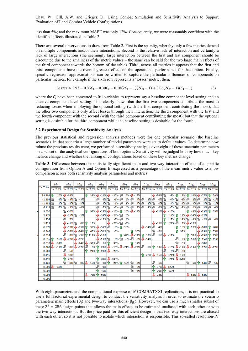
Table 3. Difference between the statistically significant main and two-way interaction effects of a specific configuration from Option A and Option B, expressed as a percentage of the mean metric value to allow comparison across both sensitivity analysis parameters and metrics

With eight parameters and the computational expense of N COMBATXXI replications, it is not practical to use a full factorial experimental design to conduct the sensitivity analysis in order to estimate the scenario parameters main effects (β ) and two-way interactions (β ). However, we can use a much smaller subset of these 2 = 256 design points that allows the main effects to be estimated unaliased with each other or with the two-way interactions. But the price paid for this efficient design is that two-way interactions are aliased with each other, so it is not possible to isolate which interaction is responsible. This so-called resolution-IV

540


fractional factorial design requires only 2 = 16 design points. We restrict attention here to the sensitivity regarding two specific configurations (the following ranking analysis will explore multiple configurations).

The regression equation is therefore:

( ) ≈ ( ) + ∑ ( ) X + ∑ ∑ ( )X X , d = 1, … , D; = , (4)

where = , denotes a specific configuration from Option A and Option B, respectively. However the aliasing structure means that only the ( ) , k = 2, … ,8 coefficients need to be estimated, since each share a common formula with three other ( ) (e. g. ( ) = ( )= ( )= ( )). The Least Squares estimates of the effects are the solutions of the linear equations = where the model matrix = ( , , . . , , , … , ).

The results of the regression technique for the case study sensitivity analysis are shown in Table 3, where the relative difference in the estimated effect sizes between the specific Option A and Option B configurations

are listed (Δ = ( ) − ( )). Only some of the metrics (e.g. toward the top of the table) are reasonably

insensitive to all eight parameters and the two-way interactions, which indicates that the choice of preferred configuration from the baseline analysis is considerably robust for these metrics. However, we note the presence of a number of two-way interactions between parameters across most other metrics, in contrast to the baseline analysis between components. Across all metrics it appears that the fifth parameter has the overall greatest effect on the sensitivity of the output values. Finally, specific regression approximations can be written to capture the particular influences of parameters on the preferred option based on particular metrics, for example if the row with mean value 0.36 represents a mission success (MS) metric, then:

( ( ) > ( )) = [ . ( . . . . . … )] (5)

which is an example of logistic regression. This is commonly expressed in the form of an odds-ratio, so that the decision sensitivity with respect to parameter (i.e. the likelihood of changing our preferred configuration when the j-th parameter changes from its low setting to its high setting) is the divergence of exp [2 −] from1 ∶ 1. For the fifth parameter we can estimate the odds-ratio as 1.22:1. The extension of this decision sensitivity setting to more than two configurations (multinomial regression) is an area for future research.

Sensitivity Analysis of Ranking Performance

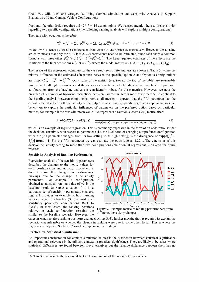
Regression analysis of the sensitivity parameters describes the changes to the metric values for each configuration individually. However, it doesn’t show the changes in performance rankings due to the change in sensitivity parameters. For example, a configuration obtained a statistical ranking value of +3 in the baseline result set versus a value of -1 in a particular set of sensitivity parameters changes. Figure 2 provides an example of how ranking values change from baseline (S00) against other sensitivity parameter combinations (S21 to S36) 3 . In most cases, the ranking positions relative to each configuration remains the similar to the baseline scenario. However, the cases in which relative ranking positions change (such as S34), further investigation is required to explain the scenario was infeasible or whether the change in ranking were due to some other factor. This is where the regression analysis in Section 3.2 would complement the findings.

Practical vs. Statistical Significance

An important consideration for combat simulation studies is the distinction between statistical significance and operational relevance in the military context, or practical significance. There are likely to be cases where statistical differences are found between two alternatives but the relative difference between them has no

3 S21 to S36 represents the fractional factorial combination of the sensitivity parameters.

Figure 2. Example metric of ranking performances from difference sensitivity changes.

541


operational impact. Currently, insights around the operational relevance of the differences between alternative configurations are considered via SME input after the simulations have been completed. This approach can lead to potential inefficiencies relating to the number of replications that need to be conducted. An alternative approach would be to identify the operational relevance threshold, or desired effect size, for each metric of interest prior to running the simulation. This may allow a smaller number of replications for each metric to be calculated using statistical techniques, assuming a pilot set of replications was run to estimate the variance of each metric. However, this approach is predicated on the assumption that the magnitude of the absolute values generated by the simulation is comparable to those expected in the real world. Anecdotal evidence indicates that combat simulations can produce trends (i.e. relative) consistent with real world military scenarios although the order of magnitude (i.e. absolute) of the results is likely to be different. Further understanding of the external validity of these models could be achieved by examining the results of simulation studies which model historical conflicts as described by Shine and Coutts (2006).

4. SUMMARY

This paper describes a COMBATXXI case study that compared land combat vehicle configurations through the use of statistical and regression analyses. A fractional factorial experimental design was used to conduct sensitivity analysis on uncertain parameters in order to determine the robustness of the baseline results. Further work is required to address issues related to the operational relevance of the deltas between sets of simulated results; the minimisation of the number of replications required for each scenario; and alternative factor screening and multiple comparison techniques.

REFERENCES

Bowley D., Castles T. and Ryan A. (2003). Constructing a SUITE of Analytical Tools: A Case Study of Military Experimentation, ASOR Bulletin, 22(4), 2-10.

Box, G.E.P. and Hunter, J.S, 1961. The 2K-P Fractional Factorial Designs, Part I. Technometrics, 3: 311-352 Cochran, W.G. and D.R. Cox, D.R. (1957). Experimental Designs. John Wiley & Sons. Cochran, W. G. (1950). The Comparison of Percentages in Matched Samples. Biometrika, 37 (3/4), 256–266 Connor, W.S. and S. Young. (1961). Fractional factorial designs for experiments with factors at two and

three levels. Applied mathematics series (58). National Bureau of Standards, Gaithersburg. Daniel, C. (1973). One-at-a-Time Plans, Journal of the American Statistical Association, 68, 353-360. Feil, M.W. (1991). A sensitivity analysis of the Janus(A) combat simulation that supports the use of Janus(A)

in army training. NPS Thesis. Friedman, M. (1937). The use of ranks to avoid the assumption of normality implicit in the analysis of

variance. Journal of the American Statistical Association. American Statistical Association. 32 (200). Kendall, M. G. (1948). Rank correlation methods, London, Griffin. Kleijnen, J.P.C. (2007). Design and Analysis of Simulation Experiments (1st ed.). Springer Publishing

Company, Incorporated. McKay, M.D., Beckman, R.J. and Conover, W.J. (1979). A Comparison of Three Methods for Selecting

Values of Input Variables in the Analysis of Output from a Computer Code. Technometrics. American Statistical Association. 21 (2): 239–245.

McNemar, Q. (1947). Note on the sampling error of the difference between correlated proportions or percentages. Psychometrika. 12 (2): 153–157

Shine, D. R. and Coutts, A. W. (2006). Establishing a Historical Baseline for Close Combat Studies – The Battle of Binh Ba. Proceedings of the 2006 Land Warfare Conference.

Training and Doctrine Command Analysis Center (TRAC) 2015, ‘COMBATXXI’, Training and Doctrine Command Analysis Center, White Sands Missile Range, viewed 26 June 2017, <http://www.trac.army.mil/COMBATXXI.pdf>

Villacorta, P. J., & Sáez, J. A. (2015). SRCS: Statistical Ranking Color Scheme for Visualizing Parameterized Multiple Pairwise Comparisons with R. R JOURNAL, 7(2), 89-104.

Wilcoxon, F. (1945). Individual comparisons by ranking methods. Biometrics Bulletin. 1 (6): 80–83.

542

Documents

Using Combat Simulation and Sensitivity Analysis to ...mssanz.org.au/modsim2017/D1/chau.pdf · Using Combat Simulation and Sensitivity Analysis to Support Evaluation of Land Combat