Using CAD to Solve Structural Geology Problems€¦ · Using CAD to Solve Structural Geology Problems Page 1 of 43 Introduction Computer-Aided Design software applications can be

Using CAD to Solve Structural Geology Problems

Page 1 of 43

Introduction Computer-Aided Design software applications can be used as a much more efficient replacement for traditional manual drafting methods. So instead of using a scale, protractor, drafting pend, etc., you can instead use CAD programs to electronically draft the solution to structural geology problems, or even compose a complete geologic map or cross-section with the application. There are many CAD applications available, costing anywhere from $5,000 to $0 (free), with varying levels of sophistication. Probably the most common is AutoCAD, however, because of the high cost of this software we will instead use a free “clone” that operates (for our purposes) just as well and is very similar in operation to AutoCAD. This application is “DraftSight”, and you may download it at no cost from the below web site:

http://www.3ds.com/products-services/draftsight-cad-software/free-download/

(or just “Google” the word “DraftSight”)

There are versions for the MacOS and Linux operating systems, however, I have only tested the Windows version (using WIN7 and WIN10) and the Linux version. I have heard from students that have used DraftSight under MacOS successfully but I can’t verify that personally. If you wish to use CAD to solve and/or compose structural geology projects please proceed to download the install file and install it on your system. There will also are several workstations with DraftSight installed in the Earth Sciences department.

Before we delve into the details of using CAD please remember this- CAD and other computer applications are just electronic replacements for manual instruments. These applications don’t solve problems for you- they just make your solution (correct or incorrect) more precise and neat. If you don’t understand the logic of the problem, CAD will not help you solve the problem.

Configuring DraftSight DraftSight needs to be configured somewhat to make it most effective for the problem at hand. Before actually starting the program consider the following questions:

1. What units are you using and what level of precision (number of decimal places) do you require? 2. How are angles formatted (DMS, radians, decimal degrees, etc.) and what level of precision is

needed? Are trends measured with azimuth or quadrant format? 3. Do you need a “grid” that functions like a virtual sheet of graph paper? Do you want to “snap”

to the grid as the cursor is moved? 4. What is your drawing scale? My recommendation is that you work in real-world coordinates,

and then scale your drawing when you produce a hard copy or PDF. You need to plan your drawing so that it fits the hard copy media size using the assigned scale. Remember that most hard copy devices have a “hardware” margin of at least 0.5 inches around the edges of the media. So printing to letter size paper (8.5 x 11.0 inches) would require a usable area of 8.0 x 10.5 inches. If you are working in real-world coordinates at a scale of 1 inch = 100 feet then the usable area would be 800 x 1050 feet.

http://www.3ds.com/products-services/draftsight-cad-software/free-download/


Page 2 of 43

5. How do you need to organize your drawing layers? Layers function like virtual transparent sheets that can be toggled on/off. For example you can use a “paper” layer to contain the dimensions of the hard copy media to use as a reference to center your drawing. This layer would never be plotted, but would be very useful for properly plotting your diagram.

6. Do you need to set entity “snap” modes? This strategy will be explained with examples in later sections.

Initial Drawing Setup At this time start the DraftSight application from the desktop or start menu. Select the “Format > Unit System” menu option. This is the “units” control command that usually needs to be set for the problem at hand. In our first example we will solve an example apparent dip problem that will use a 1:1 scale (1 plotted inch = 1 drawing unit). In Geology we normally use azimuth trend directions with north=0, east=90, south=180, etc., for angular measurements. CAD programs default to math/engineering systems with the 0 at the positive x direction (east) and positive angles increasing anticlockwise. To avoid having to constantly convert between these two systems you need to set units as depicted in Figure 1. Note that a precision of 2 decimals are set for length and decimal degree measurements. As indicated in Figure 1, set the base angle direction to north (90), and angle direction to clockwise. Note that if you use a mouse pointer left-click to set the base angle, make sure you actually click on 90 and not 91 or 88 or something close to 90 but not quite there. “90” should appear in the edit box below the graphical base angle indicator.

The setting of a “grid” with “snap” settings will be useful for aligning elements of the example problem. To do this right-click on the “grid” button at the bottom center of the window, then select “settings” to bring up the Figure 2 dialog window. Set both the horizontal and vertical grid spacing to 0.2 units as indicated. Use the same kind of procedure to set the “snap” x and y increment to 0.1 units. Make sure that the type of snap grid is “Standard” not “Radial”. Note that you can toggle any of the buttons in the bottom center of the window by left-clicking on the button. In the following examples discussed below you will see how “grid” and “snap” settings can be used effectively to aid drafting operations.

The “entity snap” settings are also important for efficient drafting of map elements. You can make the DraftSight pointer “snap” to the exact endpoint, midpoint, nearest point, etc., of an object (entity) that has already been drawn. Usually you want the “endpoint”, “nearest”, “intersection”, and “perpendicular” entity snaps set. Right-click on the “ESnap” button at the bottom center of the screen and then choose “settings” to set the entity snaps as in Figure 3.

Personal Preference Settings Personal settings are really just variations in the DraftSight user interface, however, if these modifications make you more comfortable or make the system more intuitive they are well worth experimenting with. Below are the items that I have experimented with:

1. Model Background color: This is the background color of the main “model space” drawing window. The default is black but I like white because it matches the appearance of hard copy output on white paper. You can set this with “Tools > Options > System Options > Display >


Page 3 of 43

Element Colors > Model Background Color”. One odd side effect of setting the background to “white” is that when you want to draw a black line or other object you would make the current draw color “white” – there is no “black” option. The application is smart enough to know that “white” would not display on a white background therefore it automatically switches “white” to “black”.

2. Cursor crosshair: The default cursor in the model window is a selection box but I prefer a crosshair. If you want a crosshair check the box at “Tools > Options > System Options > Display > Graphics Area > Display Cursor as Crosshair”. The size of the crosshair can be set here as well (Figure 3).

3. Selection Highlighting: by default if you move the cursor over an entity it will “highlight” to show what would be selected if you left-clicked at that position. I find this distracting so I turn this feature off, however, I leave on the entity highlighting during an active command. You can control these options from “Tools > Options > User Preferences > Entity Selection > Pre-selected Highlighting” window (Figure 4).

4. Pre-Command Selections: I prefer for left-clicks on entities to highlight so as to form a selection set that persists into the next command. If you like this setup make sure the “Enable Entity Selection before commands” checkbox is checked as in Figure 4 in the “Selection Settings” portion of the “Entity Selection” item. The default behavior in DraftSight is for a command to de-select any previously selected items.

Example Problem 1: Apparent Dip Problem The example problem reads as follows:

Given a strike and dip of 050, 40 SE find the apparent dip in a vertical section trending 110.

The first step in solving the problem will be to create a “paper” layer and draw the media edge boundary in this layer. This will allow you to properly center your problem solution on the paper. Follow the below steps outlined below.

Step 1: Create paper media boundary From the main menu choose “Format > Layer” to bring up the layer control window. Note that there is already a default layer named “0”. All new drawings will have this layer as the only layer, and it is the active layer. The active layer is the layer that new entities are assigned to by default. Use the “New” button to create a new layer and name it “paper”. Change the color to a light gray (254). Also highlight the “paper” row and click on the “activate” button to make the “paper” layer the currently active layer. The layer menu should appear similar to Figure 5. Click the “OK” button to close the layer control window.

The problem solution will be plotted on 8.5 x 11.0 inch paper (Letter size) in portrait mode (8.5 inches wide; 11.0 inches tall), however, virtually all printers have a “hardware” margin of approximately 0.25 inches around the edges of the paper so we will assume that we have a working area of 8.0 x 10.5


Page 4 of 43

inches. From the main menu select “Draw > Rectangle” (or select the rectangle button from the “draw” toolbar). Answer the prompts in the lower command line window as indicated below:

Specify start corner» 0,0

Specify opposite corner» 8,10.5

You should now see a rectangle on the screen, although part of it will probably be truncated because of the current zoom factor. To make sure the rectangle is totally displayed in the drawing window select the menu item “View > Zoom > Bounds”. You should now see the entire rectangle. The “grid” points may not show at this zoomed out scale – they will re-appear when the diagram is zoomed in later. The drawing should appear as in Figure 6. Note that there is a double-headed 90 degree arrow at the (0,0) point in the drawing. This is the User Coordinate System (UCS) icon that always indicates the direction of the positive X and Y axes in the drawing coordinate system. This is not something that you created – don’t worry it will not plot when you produce a hard copy.

Step 2: North Arrow and Reference Lines When you used the rectangle command to create the paper rectangle you indicated the opposite corners of the rectangle with absolute coordinates (0,0) and (8.0,10.5). For commands that you run in DraftSight when you are prompted for a “point” you can either use a left-click with the mouse or type a (x,y) coordinate at the command line prompt. Absolute coordinates are not the only option at the command prompt, you can also use:

Relative (x,y): @100,200 {sets a point 100 x and 200 y units relative to last point set}

Polar (distance<angle): 400<135 {sets a point 400 units at angle 135 degrees from (0,0)}

Polar relative: @400<135 {sets a point 400 units at angle 135 degrees from last point}

Let’s set the drawing “limits” to match the paper size. Use the menu item “Format > Drawing Boundary” to set the drawing bounds to (0,0) and (8.0,10.5). Create a new layer named “problem” and make it the current active layer.

At this time we need to draw a north arrow in the positive y-axis direction in the upper right corner of the paper area. Use the menu “View > Zoom > Zoom Window” to zoom into the upper right corner of the paper area. Because we set the grid spacing at 0.2 inches, you need to be able to see at least 5 vertical grid points to draw a north arrow that is 1 inch long. If you zoomed in too far use the menu item “View > Zoom > Zoom Dynamic” to properly adjust the zoom factor. Use the “Draw > Polyline” command to begin the north arrow. Before clicking on the start point make sure that the “snap” button in the bottom center is active. Proceed to click on grid points to draw an arrow like the one in Figure 7. When done right-click and select “enter” to end the command. You can also use the <Enter> key on the keyboard. Note how the cursor snaps to 0.1 unit increments as you move the cursor for precise control over point placement.


Page 5 of 43

Now it’s time to use the “text” command to put a “N” at the base of the arrow. Select the menu item “Draw > Text > SimpleNote”. Finish the command as below:

Active TextStyle: "Standard" Text height: 0.2000 Options: sEttings or Specify start position» {click at point below north arrow} Default: 0.2000 Specify height» <Enter> Default: 0 Specify text angle» <Enter>

At this point you can type in a “N”, and then type <Enter> <Enter> to finish. The “N” will probably appear offset from the arrow. Left-click on the “N” to highlight it. Left-click on the blue “handle” and move the “N” until it is centered on the arrow. Left-click at this position to finish the move. Use the “View > Zoom > Zoom Bounds” command to view all of the drawing. You should see something similar to Figure 7.

It is now time to save the project. Use “File > Save” to save the project to a file.

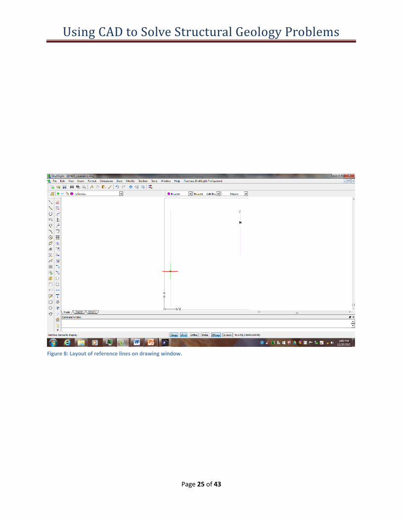
The problem solution will rely on several reference lines that are not to be plotted, therefore, we will construct them in a layer named “reference”, and we will make that layer “non-printable”. Use the layer command to create a “reference” layer, make its color magenta, and make it the active layer. Use the polyline command to draw east-west and north-south reference lines. The given information indicates that the problem will develop from left-to-right because the dip direction is to the east. Make sure that you allow the reference lines to snap to grid points to make later alignments easier. See Figure 8 for the layout of the reference lines.

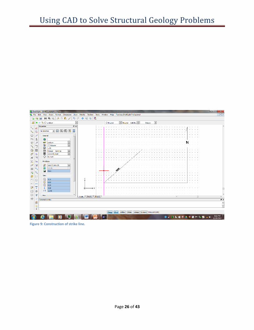
Step 3: Plot given Strike Line The strike azimuth of 050 should be plotted as a line starting at the intersection of the reference lines and extending northeast for an arbitrary distance. Make the active layer “problem”. Make sure that the “ESnap” button is “on”. Use the “Draw > Polyline” command to start a line at the intersection of the reference lines – hereafter referred to as the origin, and extend it with a second point @4.0<50 (note the use of relative polar coordinates). You should now have a strike line of azimuth 050. Use the “getdistance” command to verify that you constructed the strike line correctly: use the origin for the 1st point and the end of the strike line as the 2nd point. The output in the command window should appear as:

: getdistance Specify start point» Specify end point» Distance = 4.00, Angle in XY Plane = 50.00, Angle from XY Plane = 90.00 Delta X = 3.06, Delta Y = 2.57, Delta Z = 0.00

Use the “Draw > Text > SimpleNote” to label the strike line, but this time use a height of 0.1 and a text rotation of 50 (turn off “ESnap” before starting the command):


Page 6 of 43

Active TextStyle: "Standard" Text height: 0.20 Options: sEttings or Specify start position» {click on point close to strike line} Default: 0.20 Specify height» 0.1 Default: 90.00 Specify text angle» 50

The diagram should now appear like Figure 9.

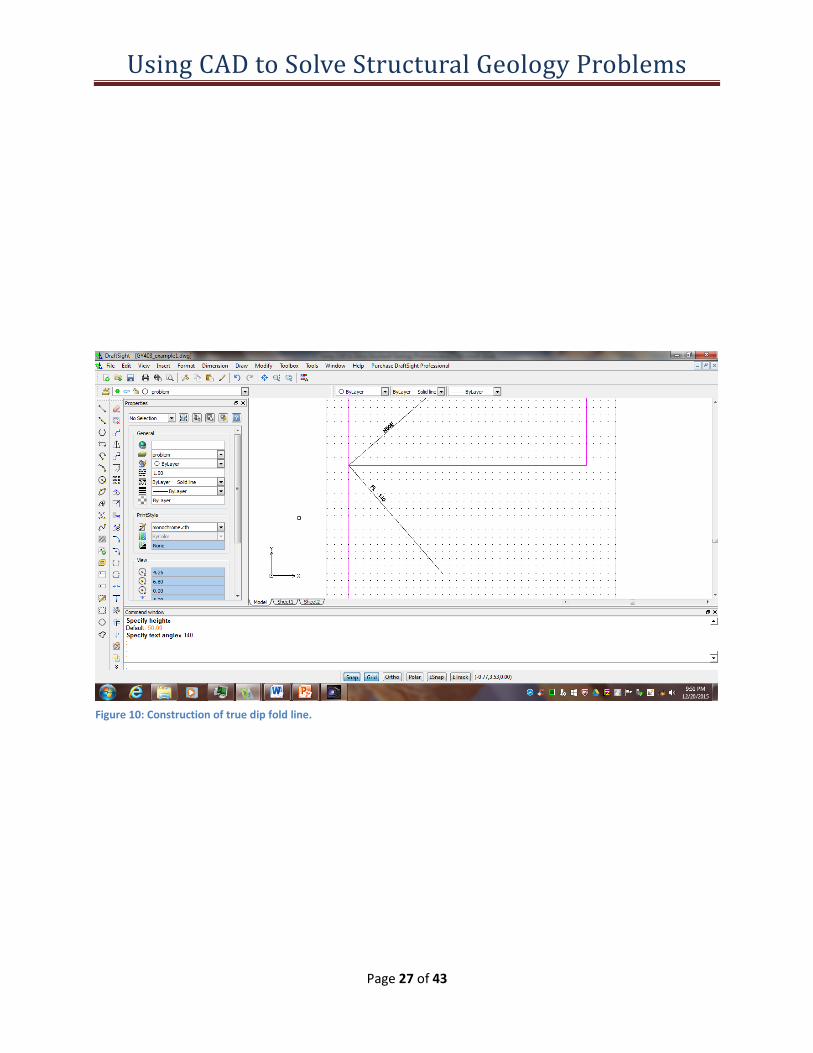
Step 4: Construct Fold Line in True Dip Direction The next step will be to construct a fold line in the true dip direction. Because the strike is 050 azimuth the true dip azimuth is perpendicular to this direction and trending to the southeast quadrant. This resolves to a 140 azimuth, so construct a polyline from the origin in this azimuth direction for a length of 4.0 units (use relative polar coordinates):

Options: Enter to continue from last point or Specify start point» <ESnaps On> {snap to origin} Options: Arc, Halfwidth, Length, Undo, Width, Enter to exit or Specify next vertex» @4<140 Options: Arc, Close, Halfwidth, Length, Undo, Width, Enter to exit or Specify next vertex» <Enter>

Now label the true dip fold line with “FL” and “140” using the “Draw > Text > SimpleNote” menu (or click on “SimpleNote” on the draw toolbar). Turn off “ESnap” before starting the “SimpleNote” command if it is on. When you are finished the diagram should now look like Figure 10.

Step 5: Construct True Dip Angle The diagram now needs to represent the true dip angle – 40 degrees – unfolded back to the horizontal surface. This is done by drawing a line oriented 40 degrees from the true dip fold line. An easy way to do this is to make an exact copy of the true dip fold line that is positioned on top of the original, and then rotate the copy using the origin as a base point 40 degrees clockwise. Select the “Modify > Copy” menu item:

Specify entities» {Left-click on true dip FL} 1 found Specify entities» <Enter> Default: Displacement Options: Displacement or Specify from point» {Left-click anywhere on diagram} Options: Enter to use first point as displacement or Specify second point» @0,0


Page 7 of 43

Default: Exit Options: Exit, Undo or Specify second point» <Enter>

This step placed a copy directly on top of the original. Now use the “Modify > Rotate” command to rotate the copy 40 degrees clockwise:

: rotate Active positive angle in CCS: DIRECTION=clockwise BASE=90.00 Specify entities» {left-click on line to rotate} 1 found Specify entities» <Enter> Specify pivot point» {snap to origin of true dip line} Default: 90.00 Options: Reference or Specify rotation angle» 40.0

This should rotate the copy of the true dip trend line 40 degrees clockwise. This represents the incline of the dipping contact rotated from a vertical plane 90 degrees to the horizontal – that is why the true dip trend is labeled as a fold line (FL).

Now let’s document that the rotated line is 40 degrees from the dip trend line with one of the “dimension” commands. Select the “Dimension > Angular” menu option:

: angledimension Options: Enter to specify vertex or Specify entity» {select the true dip trend line} Specify second line» {select the line you previously rotated} Options: Angle, Note, Text or Specify dimension position» {move the pointer to place angle text and then left-click} Dimension text : 50 {this is automatically calculated – you don’t enter anything}

This will place an angle measurement bracket between the lines. Note that the default size and precision of the angle text does not match the text you have already added. Change this with the “Modify > Properies” menu selection. This will activate the entity properties window in the left window. Modify the following properties (hover the pointer over the icon to get a “hint”):

Text Section > Text Height : change to 0.1.

Primary Unit System > Angle Precision : change to 1 decimal.


Page 8 of 43

Your diagram should appear similar to Figure 11.

Step 6: Add Vertical Depth Line Perpendicular to Dip Fold Line. The next step adds a line that represents the vertical distance from the horizontal surface at some point on the dip trend line down to the inclined dipping surface. This line must be perpendicular the dip trend line, although it may originate at any “reasonable” point on the dip trend FL. What is a “reasonable” point of origin? Far enough away from the origin point that the length of the perpendicular is long enough to be measured with enough precision – several units in this case – but not so far as to extend off the paper edge. Use the “Draw > Polyline” command to draw a line from the dipping surface line to the dip trend FL. Use an “ESnap” of “nearest” to snap to any reasonable point on the dip surface, then use “perpendicular” to snap to the FL. This is a “tricky” step so you may need some help from your instructor on this maneuver. After the perpendicular is constructed, label it using the menu command “Dimension > Aligned”:

_PARALLELDIMENSION Default: Entity Options: Entity or Specify first extension line position» e {enter “e” to select an entity} Specify entity» {left-click on perpendicular line} Options: Angle, Note, Text or Specify dimension line position» {move pointer to place text and left-click} Dimension Text : 1.6094

The label should be changed so that it is rounded to 2 decimal places, and has a text height of 0.1. Use the “Modify > Properties” menu item and look for “Primary Unit System > Precision” and “Text > Text Height”. Your diagram should look like Figure 12.

Step 7: Construct Apparent Dip Trend Fold Line. Use the polyline command to draw the apparent dip trend line at 110 azimuth. Use polar relative from the origin point with a length of 4.0 units. Instead of starting the polyline command from the main menu, use the drawing tool bar (hover the mouse pointer over the icons in the toolbar to get a “hint”). Use the “Draw > SimpleNote” command to label the new 110 azimuth apparent dip FL. Note that if you end the text label with “%%d” the degree symbol will be plotted. Use the “Modify > Properties” command to add the degree symbol to the dip trend FL also. Your diagram should resemble Figure 13.

Step 8: Construct Subsurface Structure Contour At this point we need to project a subsurface structure contour parallel to strike from the start of the dip FL perpendicular until it intersects the apparent dip FL. Use polyline and “endpoint” snap to set a start point at the end point of the dip trend / dip perpendicular intersection and set the 2nd point with a polar relative “@2.0<50” (2 units length). The new line will extend past the apparent dip FL. Use the “Modify > Trim” command to trim it to terminate exactly on the apparent dip trend line:


Page 9 of 43

: _TRIM Active settings: Projection=CCS, Edge=None Specify cutting edges ... Options: Enter to specify all entities or Specify cutting edges» {left-click on apparent dip trend FL} 1 found Options: Enter to specify all entities or Specify cutting edges» <Enter> Options: Crossing, CRossline, Project, Edge, eRase, Undo, Fence, Shift + select to extend or Specify segments to remove» {left-click on structure contour line portion past FL} Options: Crossing, CRossline, Project, Edge, eRase, Undo, Fence, Shift + select to extend or Specify segments to remove» <Enter>

The structure contour should now terminate exactly on the apparent dip trend line. The trim command can be a bit tricky to master, so if you don’t get it correct on the first attempt, select the “Edit > Undo” command to “undo” the effects and try again until you get it right. Rather than labeling the structure contour from scratch with the “Draw > Text > SimpleNote”, use the “Modify > Copy” command to copy the existing “050” label to the new structure contour. Turn off “Snap” and “ESnap” before staring the command (you can also initiate “copy” from the “modify” toolbar):

: _COPY Specify entities» {Left-click on the “050” label} 1 found Specify entities» <Enter> Default: Displacement Options: Displacement or Specify from point» {Left-click on a point near lower left of label} Options: Enter to use first point as displacement or Specify second point» {Left-click on a point above and near the structure contour} Default: Exit Options: Exit, Undo or Specify second point» <Enter>

Your diagram should now appear similar to Figure 14.

Step 9: Construct Equivalent Vertical Depth Line on Apparent Dip FL This step constructs the vertical depth line from the apparent dip FL down to the dipping surface. This line should be exactly equal to the first vertical depth perpendicular (1.61). The vertical depth line should originate where the -1.61 structure contour intersects the apparent dip trend line. It must also be perpendicular to this FL. Use the polyline command to draw a line from the intersection point at a length of 1.61 on an azimuth perpendicular to the apparent dip trend (110 -90 = 020):

: _POLYLINE


Page 10 of 43

Options: Enter to continue from last point or Specify start point» {Snap to intersection} Options: Arc, Halfwidth, Length, Undo, Width, Enter to exit or Specify next vertex» @1.61<020 Options: Arc, Close, Halfwidth, Length, Undo, Width, Enter to exit or Specify next vertex» <Enter>

This should draw the perpendicular to the exact length. Use the “Dimension > Aligned” to label this new perpendicular length.

Step 10: Connect the End of the Perpendicular to the Origin The last step connects the end of the perpendicular back to the origin so the apparent dip angle can be measured and labeled with a dimension command. Make sure that the “ESnap” is on and that “endpoint” is checked. Use the polyline command to draw the connector from the perpendicular end point to the origin. Use the “Dimension > Angular” command to label the apparent dip angle. Your diagram should appear like Figure 15. Don’t forget to label the drawing according to the standards in the lab syllabus.

Step 11: Producing a Hard Copy of the Problem Solution If you have access to a printer it is quite easy to produce hard copy output at the required scale. In this case we will output to a HP Officejet Pro 8615 Color Inkjet printer, however, the procedure would be the same for any printer. We will assume that the output media size is 8.5 x 11.0 inches (letter).

Use the “View > Zoom > Bounds” to zoom the drawing to see all elements. Make sure that all layers are turned on so that you are “seeing” all of the entities of the drawing. Turn off layers that you do not want plotted, or make them non-printable in the “Format > Layer” window.

Select the menu option “File > Print” (Figure 16). Make sure that the output device is correct- remember that many computers are connected to several different printers. Make sure that the correct orientation is indicated- the current drawing was designed for “portrait” orientation. Uncheck the “Fit to paper size” box, and then set the scale manually to “1.0 inch = 1.0 units”. This means one plotted inch on the paper equals 1.0 units used in the diagram. In the upper right you should see the green rectangle (plot entities) fit within the white rectangle (media area). Click on the “OK” button to generate the hard copy plot.

You should note that you do not have to produce a hard copy on a printer to share the results of your work. You can select “File > Print” and choose “PDF” as the output device to generate an Adobe Acrobat compatible PDF file. If you do this make sure to use the “Preview” button to preview the output before selecting “OK”. The PDF plot often needs to be shifted slightly (uncheck “print on center of paper” and adjust x and y offset values) to get a centered plot. If you print the diagram from Acrobat Reader, make sure that you use the “Actual size” option, otherwise the diagram will be scaled improperly.

In steps 1-10 when you used the “Dimension > Angular” dimension command to label an angle between two polyline entities the angle text had to be edited because the default precision setup in the “Format > Unit System” was 2 decimal places but we want 1 decimal place for labels. Although you can continue


Page 11 of 43

to use “Modify > Properties” to change the “Angle Precision” each time, there is a way to make the dimension command use 1 decimal place by default for angle text. Select the “Format > Dimension Style“ menu item. Look for the “Angular Dimension > Angular Dimension Settings” item in the window and set the “Precision” to 1 decimal place. In this window you can also change the “Text > Text Settings > Text Height” item to 0.1 to match the previous angle text. All of these changes affect the “Standard” dimension “style” that is currently in effect (see the “style” edit box at the top of the window). The next time you create an angular dimension the “Standard” dimension style settings will be used, however, they are not “retro-active” – previous dimension angle text will retain the settings that were in effect at the time they were created.

Example Problem 2: 3-point Problem A 3-point problem uses the 3D position of 3 points on a planar contact to calculate the strike and dip of the contact. Given the following information

Position relative to A Elevation

Point A N/A 700m

Point B 4100m at 247 500m

Point C 5160m at 198 200m

Use a scale of 1 inch = 1000m.

Start DraftSight and set the initial drafting settings (units, snap, etc.) as you did in the 1st example. Then follow the below steps. You will notice a difference in this problem the scale is 1 inch = 1000m so you have to decide if you are to work in paper (layout) units or the problem (world) units. For this example we will choose to work in world units.

Step 1: North Arrow and Reference Lines Draft in the north arrow and reference lines as you did in the 1st example, however, note that the given information indicated that the problem will develop from the top center of the media down toward the bottom center so the origin will be set as in Figure 17. Because everything is in world units remember to scale everything up by 1000. For example, the page media rectangle is (0,0) to (8000,10500). The North arrow text height is 0.2 * 1000 = 200. Set the grid and snap spacing to 200 and 100 respectively.

Step 2: Add Three Control Points The three control points will now be added in the required relative positions using the “Point” command. During the “point” command you can to setup the type and size of the point entities:

: _POINT Active point modes: point mode=34 point size=100.00 units Options: Multiple, Settings or Specify position» s


Page 12 of 43

Options: Multiple, Settings or Specify position» {snap to origin}

See Figure 18 for the “point settings” window. Proceed to draw polylines with the polar relative coordinates given above for points “B” and “C”. Add “points” to the ends of the polylines and label the points “B” and “C”. Add a 3rd polyline connector- the diagram should appear like Figure 19. Add labels with the “Draw > Text > Simple Note” command as indicated in the figure. Also add the dimension labels. Remember to adjust the dimension text and arrow sizes for the scale.

Step 3: Calculate and Plot Strike Line Position The strike line proportion calculation can be added to the plot as a “Draw > Text > Note” multi-line entity. Add this to the lower left portion of the diagram:

: _NOTE Active TextStyle: "Standard" Text height: 100.00 Specify first corner» {Left-click on upper left corner of text box} Options: Angle, Height, Justify, Line spacing, textSTyle, Width or Specify opposite corner» {Left-click on lower right corner of text box}

After specifying the text box you can begin to type each line followed by <enter>. When done click outside the text box area. The proportional length is 3096 so you need to plot a polyline from point C toward point A (azimuth=018) – construct this line and insert a point at the endpoint for reference. Now draw a strike line from point B through the proportional point on the A-C line that you just added. This is the strike line so label it with its azimuth value. Use a new command – “getdistance” – to calculate the azimuth of the strike line:

: getdistance Specify start point» {snap to southeast end of strike line} Specify end point» {snap to northwest end of strike line} Distance = 3151.08, Angle in XY Plane = 276.54, Angle from XY Plane = 90.00 Delta X = -3130.55, Delta Y = 359.13, Delta Z = 0.00

Note that the order of selected endpoints matters- selecting in the opposite order would yield an azimuth of 276.54 – 180 = 96.54. Because strike azimuths are read to the northern quadrant the SE-NW selection order is correct. You should now have a diagram like Figure 20. Label the proportional line with the “Dimension > Aligned” command, but before doing that consider using the “Format > Dimension Style” menu selection to change the default dimension settings to take into account the drawing coordinate system scale. Figure 21 displays the main dimension style settings window. You should look for scale dependent settings such as text height- this is changed from the default of 0.18 to 100.

Step 4: Construct True Dip Fold Line Profile To solve for the true dip angle we will use the high and low elevation point (A and C) structure contours to draw a perpendicular fold line (FL). The perpendicular map distance and the elevation difference


Page 13 of 43

between these two structure contour lines allows for the graphical or mathematical solving for the true dip angle. The simplest way to create two structure contours that are exactly parallel to the original strike line is to make copies of the original. Use the “Modify > Copy” command to copy the original strike line to points “A” and “C”. In each case make the “base” point the left endpoint of the strike line, and then snap to the “A” and “C” points for the respective destination points. Next, you need to construct a line perpendicular to the “A” and “C” structure contour lines. Do this with a “polyline” command:

: _POLYLINE Options: Enter to continue from last point or Specify start point» nea {use the “nea” override to snap to one of the structure contours} to Options: Arc, Halfwidth, Length, Undo, Width, Enter to exit or Specify next vertex» perp {use “perp” perpendicular snap override to snap to the perp. Point on the other structure contour} to Options: Arc, Close, Halfwidth, Length, Undo, Width, Enter to exit or Specify next vertex» <Enter>

Now use the “trim” command to get rid of the excess line length past the FL perpendicular. Proceed to label the FL.

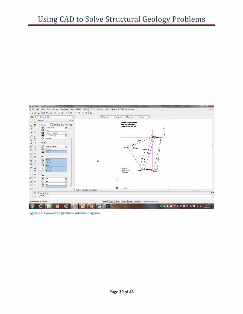
The last remaining operation is to mark off a distance on the “C” structure contour equal to the vertical elevation difference between the “A” and “C” points (700m – 200m = 500m). Use the polyline command to do this, and then connect the end of this line back to point “A”. Label the additional entities as indicated in Figure 22.

Plotting a Hard Copy Setup for printing the diagram as in Example 1 with the following exception – make the “scale” 1 inch = 1000 map units. You should then see the entity extents (green rectangle) fit within the media rectangle (white rectangle) in the upper right of the print window dialog. Click the “OK” button to plot the hard copy. See Figure 23 for the “File > Print” dialog window example.

Constructing Geologic Maps CAD programs are very useful for constructing geologic maps from field data. This section will cover some of the simple fundamental steps used in CAD to produce geologic maps. More sophisticated methods such as posting structure data automatically from a database, or georeferencing a raster image will be addressed in another document . In general the below sections will simply use CAD as electronic replacements for drafting tools.


Page 14 of 43

Inserting Station Marker Symbols on Geologic Maps Suppose that you have collected data from a closed traverse that visited outcrops where the orientation of bedding and lineation structures were measured with a pocket transit. Assume that you have been given a CAD base map to use for plotting the data. The data for the example might look like:

Leg of Traverse

Station-to-Station

Pace Bearing Distance (ft.)

Comment

1 1-2 51 342 145 st1=pine tree nearest NE corner culvert

2 2-3 58 57 165 pine tree 3 3-4 100 145 285 pine tree 4 4-5 93 234 264 st4 pine tree near picnic table 5 5-6 98 153 279 pine tree 6 6-7 72 238 204 pine tree 7 7-8 102 353 292 pine tree 8 8-1 82 10 235 pine tree

With the above data you would want to have the “Format > Units System” set to 90 for the base angle and “clockwise” for the angle direction. With this setup the above azimuth angles and distances can be easily entered as relative polar coordinates. For example, to draw in the station 1 to station 2 leg of the closed traverse:

_POLYLINE Options: Enter to continue from last point or Specify start point» Options: Arc, Halfwidth, Length, Undo, Width, Enter to exit or Specify next vertex» @145<342 Options: Arc, Close, Halfwidth, Length, Undo, Width, Enter to exit or Specify next vertex» @165<57 Options: Arc, Close, Halfwidth, Length, Undo, Width, Enter to exit or Specify next vertex» @285<145 Options: Arc, Close, Halfwidth, Length, Undo, Width, Enter to exit or Specify next vertex» @264<234 Options: Arc, Close, Halfwidth, Length, Undo, Width, Enter to exit or Specify next vertex» @279<153 Options: Arc, Close, Halfwidth, Length, Undo, Width, Enter to exit or Specify next vertex» @204<238 Options: Arc, Close, Halfwidth, Length, Undo, Width, Enter to exit or Specify next vertex» @292<353 Options: Arc, Close, Halfwidth, Length, Undo, Width, Enter to exit or Specify next vertex» @235<10 Options: Arc, Close, Halfwidth, Length, Undo, Width, Enter to exit or Specify next vertex»


Page 15 of 43

Don’t worry if your traverse strays outside the boundary of the map. You can use the “move” command to easily re-center it on the map. The next step in constructing the geologic map would be to add the structure data collected at each station on the traverse. This process is covered in the next section.

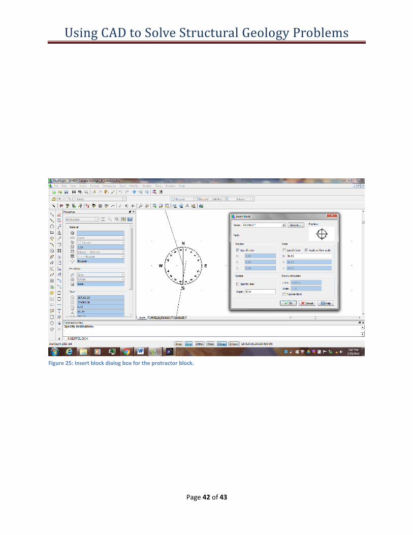
Inserting Oriented Structure Symbols (Bedding, Foliation, Lineation, etc.) on Geologic Maps Once you start drawing many structure symbols like bedding or mineral lineations you soon will figure out that there has to be a “better way” because the process is tedious and time-consuming. This is a situation that needs the application of “blocks” to save time and reduce tedium. A block is simply a collection of CAD drawing entities (lines, polylines, text, etc.) collected together in a file or memory image that can be used and re-used many times in a complex CAD file like a geologic map. If you consider it in this way it is evident that bedding, foliation, lineation symbols are all copies of the same symbol – they are just rotated to match a certain orientation, and they have a dip or plunge attribute that changes from one symbol to the next. As an example consider the CAD file displayed in Figure 24. This is the block definition of a bedding symbol (“bed.dwg”). Note that the default orientation is a strike due north and a dip angle to the east. Also note that the block attribute named “dip” is highlighted. Block attributes are text entities that prompted for when the block is inserted. If you inserted the “bed” block in a geologic map drawing you will be prompted to enter a dip value, and that value will replace the text “DIP” in Figure 24. If the block is rotated so will the attribute be rotated. The “bed” block and several other useful blocks have already been embedded into the drawing displayed in Figure 25. Use the “Insert > Block” menu selection to insert the “protract” block at the first station position in the traverse data. Use a uniform scale of 30. The structure data collected on the traverse is below:

Structure Data

Station Bedding Lineation 1 279, 50NE 045, 35 2 295, 64NE 045, 35 3 298, 68NE 045, 35 4 303, 74NE 045, 35 5 045, 35NW 045, 35 6 323, 79SW 045, 35 7 318, 86SW 045, 35 8 332, 68SW 045, 35

Now insert the “bed” block at the same point as the protractor but this time specify using a rotation later:

_INSERTBLOCK Options: Angle, reference Point, uniform Scale or Specify destination» Default: 90.0 Specify angle» 279


Page 16 of 43

Specify BlockAttribute values Default: 0 dip» 50

You should have a result like the map in Figure 26. Note that the strike line of the symbol is oriented exactly along a 279 azimuth. The dip attribute of 50 is oriented to the NE quadrant – if the dip direction had been SW you could simply rotate the block by 180 to correctly orient the symbol. If you do that you will wind up with a dip attribute rotated almost upside-down. You can fix this with the “-attedit” command:

: -attedit -EDITBLOCKATTRIBUTE Default: Yes Confirm: Edit block attributes one at a time? Specify Yes or No» y Default: * Options: * to select all blocks or Specify block(s)» * Default: * Options: * to select all attributes or Specify attribute name(s)» * Default: * Options: * to select all attribute values or Specify attribute value» 50 1 found 1 block attributes selected. Default: Next attribute Options: Height, Insertion point, Layer, LInecolor, Next attribute, text Rotation, Textstyle or Value Specify option» r {text rotation angle} Default: 9.0 Specify new text rotation» 90 {remember that angle direction is set to azimuth format} Default: Next attribute Options: Height, Insertion point, Layer, LInecolor, Next attribute, text Rotation, Textstyle or Value Specify option»

Note that all of the above operations are assuming that the base angle is set to 90 and that the angle direction is clockwise- settings appropriate for using azimuth data. You make have also noted that when you were prompted for an angle if you move the cursor the “ghost” image of the block changes its rotation. This means that if you left-click the mouse that whatever the cursor position angle is relative to the insertion point that this angle will be the rotation angle. Unfortunately this angle is always the native “mathematical” angle with “0” at east and increasing counter-clockwise. So unless you use “Format > Unit System” to set the measurement of angles back to a base of “0” and angle direction counter-clockwise you will not get a valid result with this dynamic method of specifying the rotation.


Page 17 of 43

Summary This document introduces a very small subset of commands available in CAD programs, yet the small subset of commands are able to solve a complex structural geology problem in 10 steps. You will find that there are many problems in Geology that can be efficiently solved with CAD so please experiment and consult the “Help” system built into DraftSight for more info. There are even U-tube “how to” videos online to help guide you. Below is a brief summary of commands used in the above examples:

Drawing commands

Polyline, SimpleNote, Note, Define block attribute

Dimension commands

Aligned, Angular

Modify commands

Properties, copy, move, trim, -attedit, rotate

Drawing Settings

Unit system, Grid, Snap, Entity snap

Drawing Info

Getdistance

Insert commands

block


Page 18 of 43

Figure 1: Setting the "units" system for the drawing.


Page 19 of 43

Figure 2: Setting the "grid" spacing for the drawing.


Page 20 of 43

Figure 3: Entity snap settings dialog window.


Page 21 of 43

Figure 4: Entity selection control dialog window.


Page 22 of 43

Figure 5: Layer control menu with "paper" layer active.


Page 23 of 43

Figure 6: Paper media constructed with rectangle drawing command.


Page 24 of 43

Figure 7: North arrow constructed on drawing.


Page 25 of 43

Figure 8: Layout of reference lines on drawing window.


Page 26 of 43

Figure 9: Construction of strike line.


Page 27 of 43

Figure 10: Construction of true dip fold line.


Page 28 of 43

Figure 11: Inclined dipping contact rotated to horizontal.


Page 29 of 43

Figure 12: Completion of Step 6.


Page 30 of 43

Figure 13: Completion of Step 7.


Page 31 of 43

Figure 14: Completion of Step 8 structure contour.


Page 32 of 43

Figure 15: Step 10 final solution for example problem 1.


Page 33 of 43

Figure 16: Print setup.


Page 34 of 43

Figure 17: Setup for starting 3-point example problem.


Page 35 of 43

Figure 18: Point settings window.


Page 36 of 43

Figure 19: Dimension labels for initial 3-point problem setup.


Page 37 of 43

Figure 20: Construction of strike line.


Page 38 of 43

Figure 21: Setting dimension style.


Page 39 of 43

Figure 22: Completed problem solution diagram.


Page 40 of 43

Figure 23: Print window dialog for example 2 three-point problem.


Page 41 of 43

Figure 24: Bedding block definition (bed.dwg) with dip attribute highlighted.


Page 42 of 43

Figure 25: Insert block dialog box for the protractor block.


Page 43 of 43

Figure 26: Insertion of "Bed" block with rotation of 279 and dip attribute of 50.

Documents

Using CAD to Solve Structural Geology Problems€¦ · Using CAD to Solve Structural Geology Problems Page 1 of 43 Introduction Computer-Aided Design software applications can be