Embed Size (px)
Citation preview
22 1541-1672/11/$26.00 © 2011 IEEE IEEE INTELLIGENT SYSTEMSPublished by the IEEE Computer Society
B r a i n i n f o r m a t i c s
Using Brain Imaging to Interpret Student Problem SolvingJohn R. Anderson, Shawn Betts, Jennifer L. Ferris, and Jon M. Fincham, Carnegie Mellon University
Jian Yang, Beijing University of Technology
Hidden Markov
models can be
used to combine
behavioral and
brain-imaging data
from an intelligent
tutoring system to
track mental states
during students’
problem-solving
episodes.
throughout the US, interacts with ap-proximately 500,000 students each year. Cognitive Tutors are built on cognitive models that solve problems in the same way that students do. They individu-alize instruction using two processes. The first, model tracing, uses a model of students’ problem solving to inter-pret their actions by finding a path of cognitive decisions that matches the observed actions. Given such an interpre-tation, the tutoring system provides real-time instruction individualized to where a student is in the problem. The second process, knowledge tracing, involves in-ferring which skills the student has mas-tered and then selecting new problems and instruction suited to that student’s knowledge state.
Although the principle of individual-izing instruction to a particular student holds great promise, the practice has been considerably limited by the ability to diagnose exactly what the student is thinking. The only information available
to a typical tutoring system comes from the students’ actions in the computer in-terface. The inference from such sur-face behavior to underlying thought is perilous.
We have been exploring whether multi-voxel pattern analysis (MVPA)3–8 of func-tional magnet resonance imaging (fMRI) data can be used to infer the mental states of students learning mathematics. This approach has shown considerable suc-cess in tracking static mental states such as whether a person is thinking about a location or an animal. Applying this to our case involves significant challenges not faced in many MVPA applications because it is necessary to track chang-ing student states over time. The paths of states that students take in solving prob-lems can be quite variable. Nevertheless, we have achieved relatively high accu-racy in determining what step a student is on when solving a sequence of problems and whether that step is being performed correctly.
A t Carnegie Mellon University, we have developed a successful ap-
proach to computerized instruction called Cognitive Tutors.1 These
widely used tutors focus on mathematics instruction. For instance, the Al-
gebra Tutor,2 which is currently deployed in more than 2,600 schools
IS-26-05-Ander.indd 22 15/09/11 12:12 PM
SEpTEMbEr/ocTobEr 2011 www.computer.org/intelligent 23
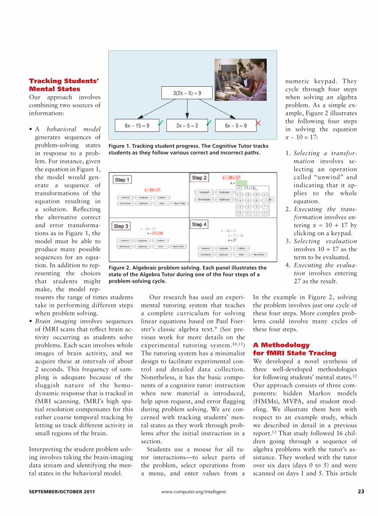
Tracking Students’ Mental StatesOur approach involves combining two sources of information:
• A behavioral model generates sequences of problem-solving states in response to a prob-lem. For instance, given the equation in Figure 1, the model would gen-erate a sequence of transformations of the equation resulting in a solution. Reflecting the alternative correct and error transforma-tions as in Figure 1, the model must be able to produce many possible sequences for an equa-tion. In addition to rep-resenting the choices that students might make, the model rep-resents the range of times students take in performing different steps when problem solving.
• Brain imaging involves sequences of fMRI scans that reflect brain ac-tivity occurring as students solve problems. Each scan involves whole images of brain activity, and we acquire these at intervals of about 2 seconds. This frequency of sam-pling is adequate because of the sluggish nature of the hemo-dynamic response that is tracked in fMRI scanning. fMRI’s high spa-tial resolution compensates for this rather coarse temporal tracking by letting us track different activity in small regions of the brain.
Interpreting the student problem solv-ing involves taking the brain-imaging data stream and identifying the men-tal states in the behavioral model.
Our research has used an experi-mental tutoring system that teaches a complete curriculum for solving linear equations based on Paul Foer-ster’s classic algebra text.9 (See pre-vious work for more details on the experimental tutoring system.10,11) The tutoring system has a minimalist design to facilitate experimental con-trol and detailed data collection. Nonetheless, it has the basic compo-nents of a cognitive tutor: instruction when new material is introduced, help upon request, and error flagging during problem solving. We are con-cerned with tracking students’ men-tal states as they work through prob-lems after the initial instruction in a section.
Students use a mouse for all tu-tor interactions—to select parts of the problem, select operations from a menu, and enter values from a
numeric keypad. They cycle through four steps when solving an algebra problem. As a simple ex-ample, Figure 2 illustrates the following four steps in solving the equation x − 10 = 17:
1. Selecting a transfor-mation involves se-lecting an operation called “unwind” and indicating that it ap-plies to the whole equation.
2. Executing the trans-formation involves en-tering x = 10 + 17 by clicking on a keypad.
3. Selecting evaluation involves 10 + 17 as the term to be evaluated.
4. Executing the evalua-tion involves entering 27 as the result.
In the example in Figure 2, solving the problem involves just one cycle of these four steps. More complex prob-lems could involve many cycles of these four steps.
A Methodology for fMRI State TracingWe developed a novel synthesis of three well-developed methodologies for following students’ mental states.12 Our approach consists of three com-ponents: hidden Markov models (HMMs), MVPA, and student mod-eling. We illustrate them here with respect to an example study, which we described in detail in a previous report.13 That study followed 16 chil-dren going through a sequence of algebra problems with the tutor’s as-sistance. They worked with the tutor over six days (days 0 to 5) and were scanned on days 1 and 5. This article
Figure 1. Tracking student progress. The Cognitive Tutor tracks students as they follow various correct and incorrect paths.
2x − 5 = 3 6x − 5 = 96x − 15 = 9
3(2x − 5) = 9
Figure 2. Algebraic problem solving. Each panel illustrates the state of the Algebra Tutor during one of the four steps of a problem-solving cycle.
IS-26-05-Ander.indd 23 15/09/11 12:12 PM
24 www.computer.org/intelligent IEEE INTELLIGENT SYSTEMS
B r a i n i n f o r m a t i c s
focuses on interpreting the students’ problem solving on day 5. To inter-pret a particular student’s behavior on day 5, we combined information from other students on day 5 and data from that student on day 1. This is similar to the development and appli-cation of Cognitive Tutors, which are deployed with statistics based on pilot students. As a particular student pro-gresses through the curriculum, Cog-nitive Tutors build a model of that student.
Our brain-imaging data come from blocks, which are sequences of about six problems. We used the brain- imaging data to determine what prob-lem a student is working on and what step the student is performing within a problem. Determining what step the student is on is referred to as the seg-mentation goal. We also used the imag-ing data to determine whether that step is being performed correctly. We refer to this as the diagnosis goal. We chose these goals because there is a hard def-inition of ground truth here—namely, the computer logs of the students’ progress through these problems.
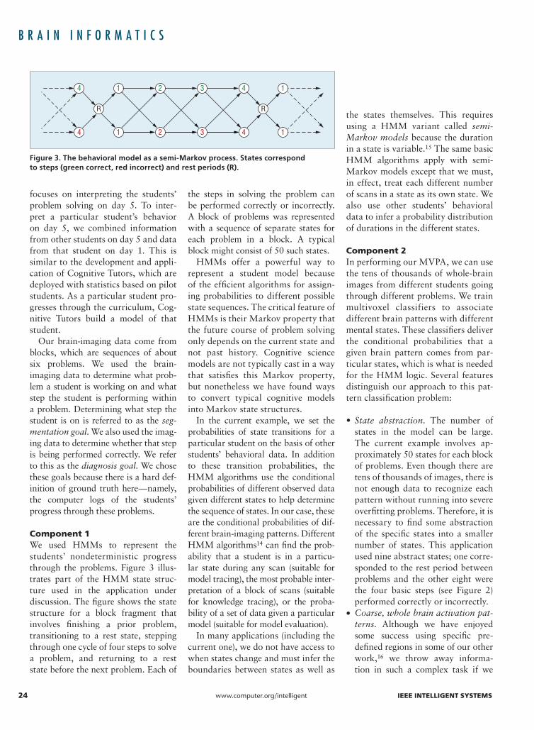
component 1We used HMMs to represent the students’ nondeterministic progress through the problems. Figure 3 illus-trates part of the HMM state struc-ture used in the application under discussion. The figure shows the state structure for a block fragment that involves finishing a prior problem, transitioning to a rest state, stepping through one cycle of four steps to solve a problem, and returning to a rest state before the next problem. Each of
the steps in solving the problem can be performed correctly or incorrectly. A block of problems was represented with a sequence of separate states for each problem in a block. A typical block might consist of 50 such states.
HMMs offer a powerful way to represent a student model because of the efficient algorithms for assign-ing probabilities to different possible state sequences. The critical feature of HMMs is their Markov property that the future course of problem solving only depends on the current state and not past history. Cognitive science models are not typically cast in a way that satisfies this Markov property, but nonetheless we have found ways to convert typical cognitive models into Markov state structures.
In the current example, we set the probabilities of state transitions for a particular student on the basis of other students’ behavioral data. In addition to these transition probabilities, the HMM algorithms use the conditional probabilities of different observed data given different states to help determine the sequence of states. In our case, these are the conditional probabilities of dif-ferent brain-imaging patterns. Different HMM algorithms14 can find the prob-ability that a student is in a particu-lar state during any scan (suitable for model tracing), the most probable inter-pretation of a block of scans (suitable for knowledge tracing), or the proba-bility of a set of data given a particular model (suitable for model evaluation).
In many applications (including the current one), we do not have access to when states change and must infer the boundaries between states as well as
the states themselves. This requires using a HMM variant called semi-Markov models because the duration in a state is variable.15 The same basic HMM algorithms apply with semi-Markov models except that we must, in effect, treat each different number of scans in a state as its own state. We also use other students’ behavioral data to infer a probability distribution of durations in the different states.
component 2In performing our MVPA, we can use the tens of thousands of whole-brain images from different students going through different problems. We train multivoxel classifiers to associate different brain patterns with different mental states. These classifiers deliver the conditional probabilities that a given brain pattern comes from par-ticular states, which is what is needed for the HMM logic. Several features distinguish our approach to this pat-tern classification problem:
• State abstraction. The number of states in the model can be large. The current example involves ap-proximately 50 states for each block of problems. Even though there are tens of thousands of images, there is not enough data to recognize each pattern without running into severe overfitting problems. Therefore, it is necessary to find some abstraction of the specific states into a smaller number of states. This application used nine abstract states; one corre-sponded to the rest period between problems and the other eight were the four basic steps (see Figure 2) performed correctly or incorrectly.
• Coarse, whole brain activation pat-terns. Although we have enjoyed some success using specific pre-defined regions in some of our other work,16 we throw away informa-tion in such a complex task if we
34
4
21
321
R
4
4
1
1
R
Figure 3. The behavioral model as a semi-Markov process. States correspond to steps (green correct, red incorrect) and rest periods (R).
IS-26-05-Ander.indd 24 15/09/11 12:12 PM
SEpTEMbEr/ocTobEr 2011 www.computer.org/intelligent 25
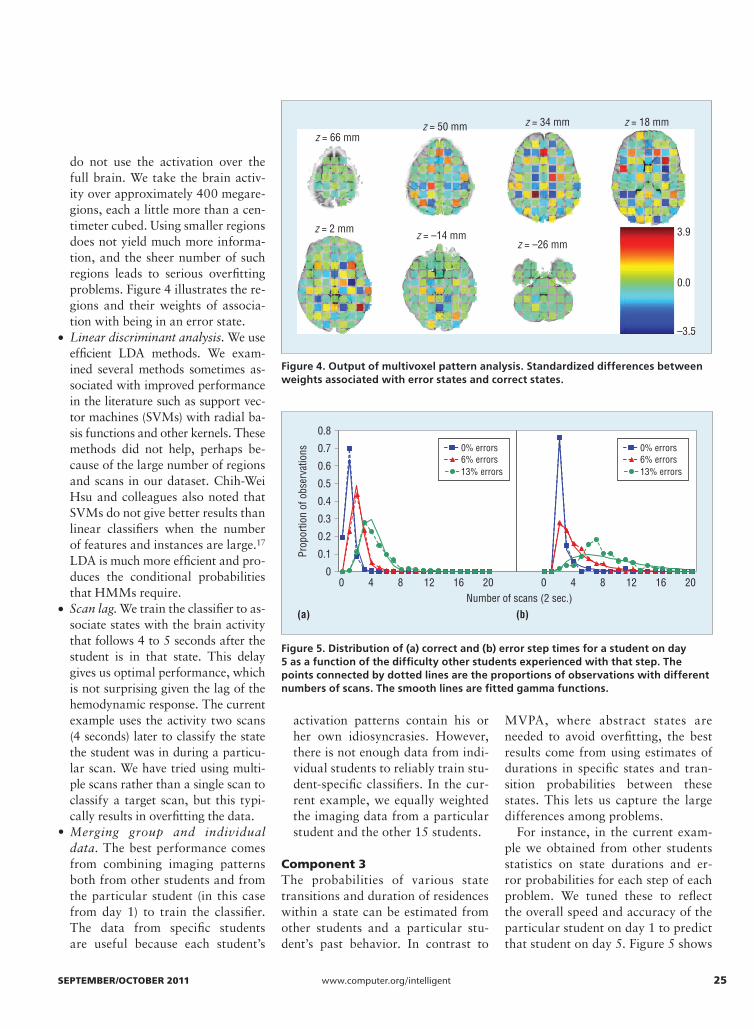
do not use the activation over the full brain. We take the brain activ-ity over approximately 400 megare-gions, each a little more than a cen-timeter cubed. Using smaller regions does not yield much more informa-tion, and the sheer number of such regions leads to serious overfitting problems. Figure 4 illustrates the re-gions and their weights of associa-tion with being in an error state.
• Linear discriminant analysis. We use efficient LDA methods. We exam-ined several methods sometimes as-sociated with improved performance in the literature such as support vec-tor machines (SVMs) with radial ba-sis functions and other kernels. These methods did not help, perhaps be-cause of the large number of regions and scans in our dataset. Chih-Wei Hsu and colleagues also noted that SVMs do not give better results than linear classifiers when the number of features and instances are large.17 LDA is much more efficient and pro-duces the conditional probabilities that HMMs require.
• Scan lag. We train the classifier to as-sociate states with the brain activity that follows 4 to 5 seconds after the student is in that state. This delay gives us optimal performance, which is not surprising given the lag of the hemodynamic response. The current example uses the activity two scans (4 seconds) later to classify the state the student was in during a particu-lar scan. We have tried using multi-ple scans rather than a single scan to classify a target scan, but this typi-cally results in overfitting the data.
• Merging group and individual data. The best performance comes from combining imaging patterns both from other students and from the particular student (in this case from day 1) to train the classifier. The data from specific students are useful because each student’s
activation patterns contain his or her own idiosyncrasies. However, there is not enough data from indi-vidual students to reliably train stu-dent-specific classifiers. In the cur-rent example, we equally weighted the imaging data from a particular student and the other 15 students.
component 3The probabilities of various state transitions and duration of residences within a state can be estimated from other students and a particular stu-dent’s past behavior. In contrast to
MVPA, where abstract states are needed to avoid overfitting, the best results come from using estimates of durations in specific states and tran-sition probabilities between these states. This lets us capture the large differences among problems.
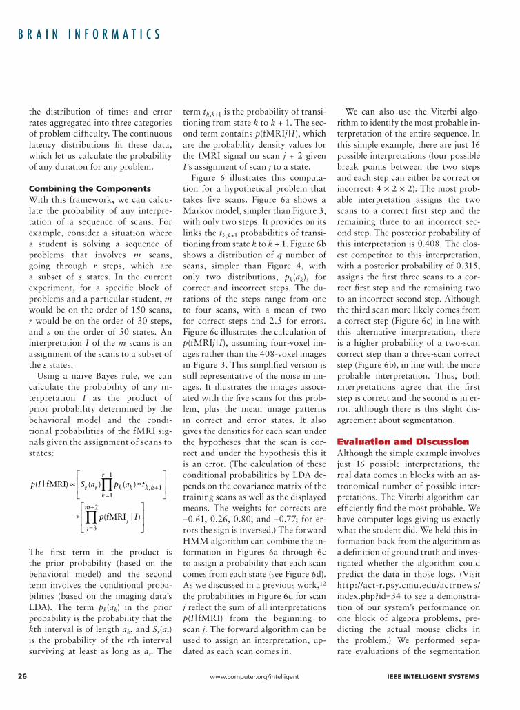
For instance, in the current exam-ple we obtained from other students statistics on state durations and er-ror probabilities for each step of each problem. We tuned these to reflect the overall speed and accuracy of the particular student on day 1 to predict that student on day 5. Figure 5 shows
z = 66 mm
z = 2 mm z = –14 mmz = –26 mm
3.9
0.0
–3.5
z = 50 mm z = 34 mm z = 18 mm
Figure 4. Output of multivoxel pattern analysis. Standardized differences between weights associated with error states and correct states.
0
(a) (b)
0.1
0.2
0.3
0.4
0.5
0.6
0.7
0.8
0 4 8 12 16 20 0 4 8 12 16 20
Prop
ortio
n of
obs
erva
tions
Number of scans (2 sec.)
0% errors6% errors13% errors
0% errors6% errors13% errors
Figure 5. Distribution of (a) correct and (b) error step times for a student on day 5 as a function of the difficulty other students experienced with that step. The points connected by dotted lines are the proportions of observations with different numbers of scans. The smooth lines are fitted gamma functions.
IS-26-05-Ander.indd 25 15/09/11 12:12 PM
26 www.computer.org/intelligent IEEE INTELLIGENT SYSTEMS
B r a i n i n f o r m a t i c s
the distribution of times and error rates aggregated into three categories of problem difficulty. The continuous latency distributions fit these data, which let us calculate the probability of any duration for any problem.
combining the componentsWith this framework, we can calcu-late the probability of any interpre-tation of a sequence of scans. For example, consider a situation where a student is solving a sequence of problems that involves m scans, going through r steps, which are a subset of s states. In the current experiment, for a specific block of problems and a particular student, m would be on the order of 150 scans, r would be on the order of 30 steps, and s on the order of 50 states. An interpretation I of the m scans is an assignment of the scans to a subset of the s states.
Using a naive Bayes rule, we can calculate the probability of any in-terpretation I as the product of prior probability determined by the behavioral model and the condi-tional probabilities of the fMRI sig-nals given the assignment of scans to states:
p I S a p a tr r k k k kk
r
( | ) ( ) ( ) ,fMRI ∝ ∗
+
=
−
∏ 11
1
∗
=
+
∏ p Ijj
m
( | )fMRI3
2
The first term in the product is the prior probability (based on the behavioral model) and the second term involves the conditional proba-bilities (based on the imaging data’s LDA). The term pk(ak) in the prior probability is the probability that the kth interval is of length ak, and Sr(ar) is the probability of the rth interval surviving at least as long as ar. The
term tk,k+1 is the probability of transi-tioning from state k to k + 1. The sec-ond term contains p(fMRIj | I), which are the probability density values for the fMRI signal on scan j + 2 given I’s assignment of scan j to a state.
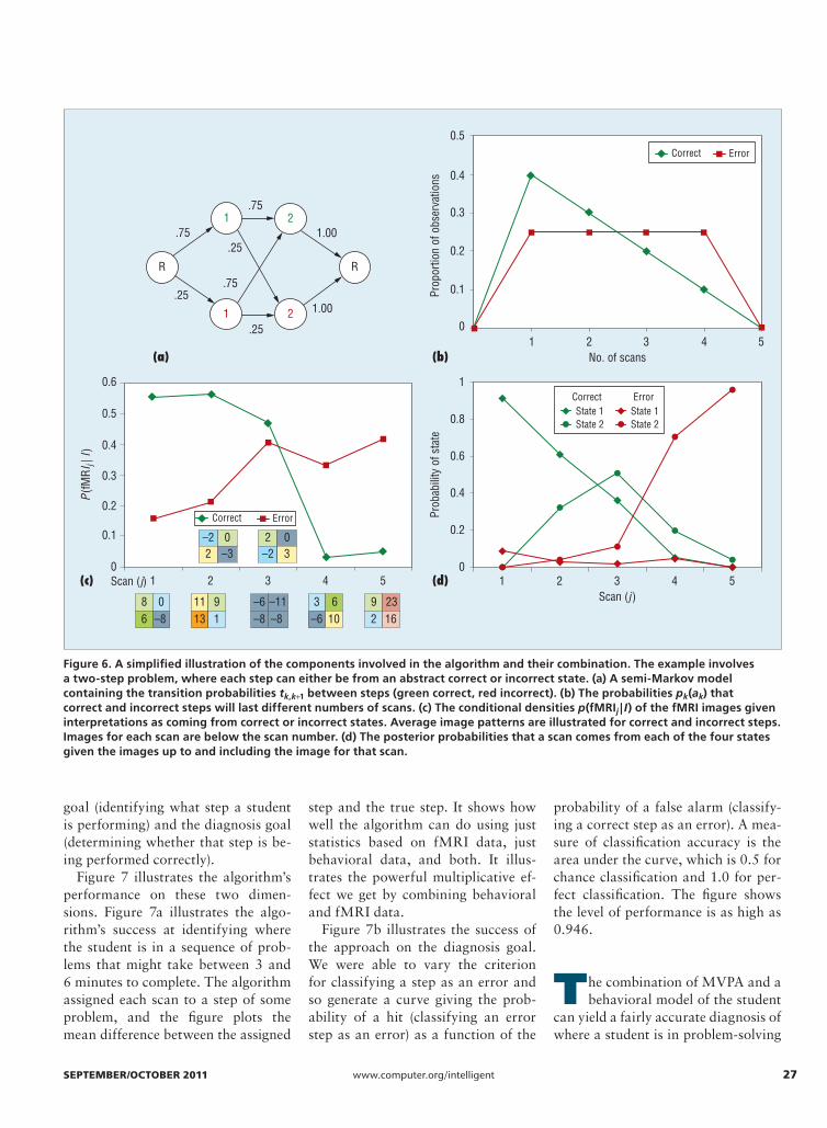
Figure 6 illustrates this computa-tion for a hypothetical problem that takes five scans. Figure 6a shows a Markov model, simpler than Figure 3, with only two steps. It provides on its links the tk,k+1 probabilities of transi-tioning from state k to k + 1. Figure 6b shows a distribution of q number of scans, simpler than Figure 4, with only two distributions, pk(ak), for correct and incorrect steps. The du-rations of the steps range from one to four scans, with a mean of two for correct steps and 2.5 for errors. Figure 6c illustrates the calculation of p(fMRIj | I), assuming four-voxel im-ages rather than the 408-voxel images in Figure 3. This simplified version is still representative of the noise in im-ages. It illustrates the images associ-ated with the five scans for this prob-lem, plus the mean image patterns in correct and error states. It also gives the densities for each scan under the hypotheses that the scan is cor-rect and under the hypothesis this it is an error. (The calculation of these conditional probabilities by LDA de-pends on the covariance matrix of the training scans as well as the displayed means. The weights for corrects are –0.61, 0.26, 0.80, and –0.77; for er-rors the sign is inversed.) The forward HMM algorithm can combine the in-formation in Figures 6a through 6c to assign a probability that each scan comes from each state (see Figure 6d). As we discussed in a previous work,12 the probabilities in Figure 6d for scan j reflect the sum of all interpretations p(I | fMRI) from the beginning to scan j. The forward algorithm can be used to assign an interpretation, up-dated as each scan comes in.
We can also use the Viterbi algo-rithm to identify the most probable in-terpretation of the entire sequence. In this simple example, there are just 16 possible interpretations (four possible break points between the two steps and each step can either be correct or incorrect: 4 × 2 × 2). The most prob-able interpretation assigns the two scans to a correct first step and the remaining three to an incorrect sec-ond step. The posterior probability of this interpretation is 0.408. The clos-est competitor to this interpretation, with a posterior probability of 0.315, assigns the first three scans to a cor-rect first step and the remaining two to an incorrect second step. Although the third scan more likely comes from a correct step (Figure 6c) in line with this alternative interpretation, there is a higher probability of a two-scan correct step than a three-scan correct step (Figure 6b), in line with the more probable interpretation. Thus, both interpretations agree that the first step is correct and the second is in er-ror, although there is this slight dis-agreement about segmentation.
Evaluation and DiscussionAlthough the simple example involves just 16 possible interpretations, the real data comes in blocks with an as-tronomical number of possible inter-pretations. The Viterbi algorithm can efficiently find the most probable. We have computer logs giving us exactly what the student did. We held this in-formation back from the algorithm as a definition of ground truth and inves-tigated whether the algorithm could predict the data in those logs. (Visit http://act-r.psy.cmu.edu/actrnews/ index.php?id=34 to see a demonstra-tion of our system’s performance on one block of algebra problems, pre-dicting the actual mouse clicks in the problem.) We performed sepa-rate evaluations of the segmentation
IS-26-05-Ander.indd 26 15/09/11 12:12 PM
SEpTEMbEr/ocTobEr 2011 www.computer.org/intelligent 27
goal (identifying what step a student is performing) and the diagnosis goal (determining whether that step is be-ing performed correctly).
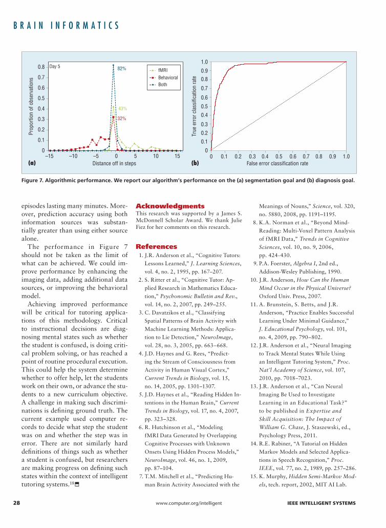
Figure 7 illustrates the algorithm’s performance on these two dimen-sions. Figure 7a illustrates the algo-rithm’s success at identifying where the student is in a sequence of prob-lems that might take between 3 and 6 minutes to complete. The algorithm assigned each scan to a step of some problem, and the figure plots the mean difference between the assigned
step and the true step. It shows how well the algorithm can do using just statistics based on fMRI data, just behavioral data, and both. It illus-trates the powerful multiplicative ef-fect we get by combining behavioral and fMRI data.
Figure 7b illustrates the success of the approach on the diagnosis goal. We were able to vary the criterion for classifying a step as an error and so generate a curve giving the prob-ability of a hit (classifying an error step as an error) as a function of the
probability of a false alarm (classify-ing a correct step as an error). A mea-sure of classification accuracy is the area under the curve, which is 0.5 for chance classification and 1.0 for per-fect classification. The figure shows the level of performance is as high as 0.946.
The combination of MVPA and a behavioral model of the student
can yield a fairly accurate diagnosis of where a student is in problem-solving
0
0.2
0.4
0.6
0.8
1
1 2 3 4 5
Prob
abili
ty o
f sta
te
Scan (j )
State 1Correct
Correct
Error
Error
State 1State 2 State 2
0
0.2
0.1
0.3
0.4
0.5
0.6
1 2 3 4 5
P(fM
RIj |
I)
Scan (j)
0
0.1
0.2
0.3
0.4
0.5
1 2 3 4 5
Prop
ortio
n of
obs
erva
tions
No. of scans
Correct Error
(c) (d)
(b)(a)
8 06
11 913 1
–6 –11–8 –8–8
3 6–6 10
9 232 16
–2 02 –3
2 0–2 3
1 2
RR
.75
.75
1.00
1.00
.75
.25
.25
.2521
Figure 6. A simplified illustration of the components involved in the algorithm and their combination. The example involves a two-step problem, where each step can either be from an abstract correct or incorrect state. (a) A semi-Markov model containing the transition probabilities tk,k+1 between steps (green correct, red incorrect). (b) The probabilities pk(ak) that correct and incorrect steps will last different numbers of scans. (c) The conditional densities p(fMRIj | I) of the fMRI images given interpretations as coming from correct or incorrect states. Average image patterns are illustrated for correct and incorrect steps. Images for each scan are below the scan number. (d) The posterior probabilities that a scan comes from each of the four states given the images up to and including the image for that scan.
IS-26-05-Ander.indd 27 15/09/11 12:12 PM
28 www.computer.org/intelligent IEEE INTELLIGENT SYSTEMS
B r a i n i n f o r m a t i c s
episodes lasting many minutes. More-over, prediction accuracy using both information sources was substan-tially greater than using either source alone.
The performance in Figure 7 should not be taken as the limit of what can be achieved. We could im-prove performance by enhancing the imaging data, adding additional data sources, or improving the behavioral model.
Achieving improved performance will be critical for tutoring applica-tions of this methodology. Critical to instructional decisions are diag-nosing mental states such as whether the student is confused, is doing criti-cal problem solving, or has reached a point of routine procedural execution. This could help the system determine whether to offer help, let the students work on their own, or advance the stu-dents to a new curriculum objective. A challenge in making such discrimi-nations is defining ground truth. The current example used computer re-cords to decide what step the student was on and whether the step was in error. There are not similarly hard definitions of things such as whether a student is confused, but researchers are making progress on defining such states within the context of intelligent tutoring systems.18
AcknowledgmentsThis research was supported by a James S. McDonnell Scholar Award. We thank Julie Fiez for her comments on this research.
References1. J.R. Anderson et al., “Cognitive Tutors:
Lessons Learned,” J. Learning Sciences,
vol. 4, no. 2, 1995, pp. 167–207.
2. S. Ritter et al., “Cognitive Tutor: Ap-
plied Research in Mathematics Educa-
tion,” Psychonomic Bulletin and Rev.,
vol. 14, no. 2, 2007, pp. 249–255.
3. C. Davatzikos et al., “Classifying
Spatial Patterns of Brain Activity with
Machine Learning Methods: Applica-
tion to Lie Detection,” NeuroImage,
vol. 28, no. 3, 2005, pp. 663–668.
4. J.D. Haynes and G. Rees, “Predict-
ing the Stream of Consciousness from
Activity in Human Visual Cortex,”
Current Trends in Biology, vol. 15,
no. 14, 2005, pp. 1301–1307.
5. J.D. Haynes et al., “Reading Hidden In-
tentions in the Human Brain,” Current
Trends in Biology, vol. 17, no. 4, 2007,
pp. 323–328.
6. R. Hutchinson et al., “Modeling
fMRI Data Generated by Overlapping
Cognitive Processes with Unknown
Onsets Using Hidden Process Models,”
NeuroImage, vol. 46, no. 1, 2009,
pp. 87–104.
7. T.M. Mitchell et al., “Predicting Hu-
man Brain Activity Associated with the
Meanings of Nouns,” Science, vol. 320,
no. 5880, 2008, pp. 1191–1195.
8. K.A. Norman et al., “Beyond Mind-
Reading: Multi-Voxel Pattern Analysis
of fMRI Data,” Trends in Cognitive
Sciences, vol. 10, no. 9, 2006,
pp. 424-430.
9. P.A. Foerster, Algebra I, 2nd ed.,
Addison-Wesley Publishing, 1990.
10. J.R. Anderson, How Can the Human
Mind Occur in the Physical Universe?
Oxford Univ. Press, 2007.
11. A. Brunstein, S. Betts, and J.R.
Anderson, “Practice Enables Successful
Learning Under Minimal Guidance,”
J. Educational Psychology, vol. 101,
no. 4, 2009, pp. 790–802.
12. J.R. Anderson et al., “Neural Imaging
to Track Mental States While Using
an Intelligent Tutoring System,” Proc.
Nat’l Academy of Science, vol. 107,
2010, pp. 7018–7023.
13. J.R. Anderson et al., “Can Neural
Imaging Be Used to Investigate
Learning in an Educational Task?”
to be published in Expertise and
Skill Acquisition: The Impact of
William G. Chase, J. Staszewski, ed.,
Psychology Press, 2011.
14. R.E. Rabiner, “A Tutorial on Hidden
Markov Models and Selected Applica-
tions in Speech Recognition,” Proc.
IEEE, vol. 77, no. 2, 1989, pp. 257–286.
15. K. Murphy, Hidden Semi-Markov Mod-
els, tech. report, 2002, MIT AI Lab.
0
0.1
0.2
0.3
0.4
0.5
0.6
0.7
0.8
–15 –10 –5 0 5 10 15
Prop
ortio
n of
obs
erva
tions
Distance off in steps
Day 5fMRIBehavioralBoth
32%
43%
82%
0
0.1
0.2
0.3
0.4
0.5
0.6
0.7
0.80.9
1.0
True
err
or c
lass
ifica
tion
rate
False error classification rate0 0.1 0.2 0.3 0.4 0.5 0.6 0.7 0.8 0.9 1.0
(a) (b)
Figure 7. Algorithmic performance. We report our algorithm’s performance on the (a) segmentation goal and (b) diagnosis goal.
IS-26-05-Ander.indd 28 15/09/11 12:13 PM

SEpTEMbEr/ocTobEr 2011 www.computer.org/intelligent 29
16. J.R. Anderson et al., “Tracking Chil-
dren’s Mental States while Solving
Algebra Equations,” to be published
in Human Brain Mapping, 2011.
17. C.W. Hsu, C.C. Chang, and C.J. Lin,
“A Practical Guide to Support Vector
Classification,” Dept. of Computer
Science and Information Eng., Nat’l
Taiwan Univ., 2009.
18. A.C. Graesser et al., “The Relation-
ship Between Affect States and Dia-
logue Patterns During Interactions
with AutoTutor,” J. Interactive
Learning Research, vol. 19, 2008,
pp. 293–312.
t h e a u t h o r sJohn r. Anderson is the Richard King Mellon Professor of Psychology and Computer Science at Carnegie Mellon University. He is known for developing ACT-R, which is the most widely used cognitive architecture in cognitive science, and as an early leader in re-search on intelligent tutoring systems. Anderson has a PhD in psychology from Stanford University. He is a past-president of the Cognitive Science Society and has been elected to the American Academy of Arts and Sciences, the National Academy of Sciences, and the American Philosophical Society. Contact him at [email protected].
Shawn betts is a research programmer at Carnegie Mellon University. His research inter-ests include the design of instructional software. Betts has a BS in computer science from Simon Fraser University. Contact him at [email protected].
Jennifer L. Ferris is a research associate at Carnegie Mellon University. Her research in-terests include the learning of mathematics. Ferris has a MA in psychology from Bucknell University. Contact her at [email protected].
Jon M. Fincham is a research psychologist at Carnegie Mellon University. His research interests include the neural imaging and simulation modeling of complex cognitive pro-cesses. Fincham has PhD in psychology from Carnegie Mellon University. Contact him at [email protected].
Jian Yang is a lector in the International WIC Institute at the Beijing University of Tech-nology. His research interests include manifold learning, machine learning, data mining, fMRI data analysis, and Web intelligence. Yang has a PhD in pattern recognition and in-telligent system from the Institute of Automation, Chinese Academy of Sciences. Contact him at [email protected].
Selected CS articles and columns are also available for free at
http://ComputingNow.computer.org.
Let us bring technology news to you.
Subscribe to our daily newsfeed
http://computingnow.computer.org
IS-26-05-Ander.indd 29 15/09/11 12:13 PM