Using a Model to Compute the Optimal Schedule of …cognitrn.psych.indiana.edu/rgoldsto/courses/cogsci...Using a Model to Compute the Optimal Schedule of Practice Philip I. Pavlik,

Using a Model to Compute the Optimal Schedule of Practice

Philip I. Pavlik, Jr. and John R. AndersonCarnegie Mellon University

By balancing the spacing effect against the effects of recency and frequency, this paper explains howpractice may be scheduled to maximize learning and retention. In an experiment, an optimized conditionusing an algorithm determined with this method was compared with other conditions. The optimizedcondition showed significant benefits with large effect sizes for both improved recall and recall latency.The optimization method achieved these benefits by using a modeling approach to develop a quantitativealgorithm, which dynamically maximizes learning by determining for each item when the balancebetween increasing temporal spacing (that causes better long-term recall) and decreasing temporalspacing (that reduces the failure related time cost of each practice) means that the item is at the spacinginterval where long-term gain per unit of practice time is maximal. As practice repetitions accumulate foreach item, items become stable in memory and this optimal interval increases.

Keywords: memory, practice, paired-associate, efficiency, spacing effect

Since the end of the 19th century researchers have tried todescribe the best way to practice to enhance learning and retention.This work began around the time of Ebbinghaus (1913/1885), whofocused on how the history of practice for items controls the futurestrength or retrievability of memories formed. Ebbinghaus’ re-search helped to establish methods for the scientific study ofmemory and demonstrated memory effects that are still studiedtoday. Although many of his investigations demonstrated the ef-fects of frequency and recency, first listed as principles of associ-ation by Thomas Brown in the early 19th century (Murphy &Kovach, 1972), he is also credited with uncovering the “spacingeffect” because he discovered that by interspersing sleep periodsbetween study sessions subsequent performance was improvedcompared to a contiguous session.

Since Ebbinghaus’ (1913/1885) results, researchers have fo-cused on the obvious educational implication of these findings,with particular emphasis on the spacing effect because of itsapparent ability to produce more durable learning. Indeed, a cen-tral theoretical question in this paper, whether long temporal

intervals between practices are always optimal for learning orwhether initial practice requires shorter spacing, was first debatedby Steffens (1900) and Jost (1897) according to a review on theliterature by Ruch (1928). Although Steffens advocated widerspacing overall, Jost advocated narrower initial spacing, and thedebate on this issue continues today. It is in the context of thismore than century long effort to understand a general solution tothe question of optimal practice scheduling that we will begin byintroducing an understanding of the “spacing effect” and its im-plications.

The “spacing effect” is the often found and widely recognizedlearning advantage of having intervals of time between repetitionsof a skilled performance, particularly when the skilled perfor-mance involves factual recall (Dempster, 1996). Although someauthors such as Underwood, Kapelak, and Malmi (1976) havedistinguished the spacing effect from the lag effect (which speci-fies that increasing the duration of the spaced lag between repeti-tions increase the benefit of spacing), this paper assumes thatspacing effects are function of lag, particularly for fact learning.Whereas the spacing effect in fact learning has been well knownsince Ebbinghaus (1913/1885), more recent work has clarified howit functions by demonstrating that there are two important inter-actions to consider when applying spacing:

1. Several authors have shown that as retention intervalincreases, the benefit of spacing is larger (implying thatspacing improves the durability of learning). Thisretention-interval-by-spacing interaction has been shownover short time scales ranging from seconds and minutes(Glenberg, 1976; Peterson, Wampler, Kirkpatrick, &Saltzman, 1963) and over days and months (Bahrick,1979; Fishman, Keller, & Atkinson, 1969; Pashler,Zarow, & Triplett, 2003; Pavlik, 2005). Because theinteraction of spacing and retention interval is often quitelarge in the above studies (e.g., Pashler et al., 2003), it iscrucial to account for when scheduling practice.

Philip I. Pavlik, Jr., Human Computer Interaction Institute, CarnegieMellon University, Pittsburgh; John R. Anderson, Department of Psychol-ogy, Carnegie Mellon University, Pittsburgh.

This research was supported by NIH training Grant MH 62011 andNIMH R01 MH 68234 and a grant from Ronald Zdrojkowski for educa-tional research. Data from the experiment are available by contacting thefirst author by email. Researchers interested in implementing the systemdescribed in this paper are invited to contact the first author for a copy ofthe current full system (posted for testing at www.optimallearning.org).Alternatively, interested researchers may request copies of the Java pro-gramming language functions that instantiate the ACT-R model and choosethe most optimal item for practice based on that model.

Correspondence concerning this article should be addressed toPhilip I. Pavlik, Jr., Human Computer Interaction Institute, CarnegieMellon University, 5000 Forbes Ave, Pittsburgh, PA 15213. E-mail:[email protected]

Journal of Experimental Psychology: Applied Copyright 2008 by the American Psychological Association2008, Vol. 14, No. 2, 101–117 1076-898X/08/$12.00 DOI: 10.1037/1076-898X.14.2.101

101

2. Researchers have shown that spaced practice has a cu-mulative effect such that each additional spaced practiceprovides an additional advantage (spacing by practicequantity interaction) (Pavlik & Anderson, 2005; Under-wood, 1970). This interaction with practice quantityhighlights the continuing importance of spaced practiceas practice accumulates.

The main effect of spacing and these interactions stronglysuggest that spacing is important to take advantage of whenscheduling practice, that spacing does continue to apply whenfrequency increases, and that these benefits are a function of theretention interval.

On the other hand, wide spacings can result in a significantslowing of the rate at which material can be learned because of thegreater forgetting between repetitions. This is particularly true forpractice procedures that include a test of the material being learnedfor each trial. For example, a typical practice procedure involves atest followed by a review presentation if the item cannot berecalled (referred to in this paper as a recall-or-restudy trial or adrill trial). At short spacing, the participant is likely to quicklyrecall the item and forgo the need for a review presentation(benefits of recency). This drill task should be an effective way totrain items because testing has often been shown to be a particu-larly effective means of practice (e.g., Carrier & Pashler, 1992).Thus, it is necessary to have a method for finding the spacing thatproduces the most learning gains with the least slowing of learningrate.

Other researchers of optimal scheduling issues have tried tomove forward on the problem by comparing alternative schedulesin experiments to determine empirically what sorts of schedulesare optimal for learning (Balota, Duchek, Sergent-Marshall, &Roediger, 2006; Cull, 2000; Cull, Shaughnessy, & Zechmeister,1996; Landauer & Bjork, 1978; Rea & Modigliani, 1985). Thesestudies provide data that are useful in helping us understand theoptimal scheduling of practice, but they do not provide a system-atic method of computing schedules such as is presented in thispaper. For example, Karpicke and Roediger (2007) tested thetheory that expanding spacing is optimal by comparing a conditionwith expanding spacing of practice (where practice is initiallynarrow but increases with each new repetition) to a condition withequally spaced practice. In these comparisons, they showed thatthe expanding spacing schedule only produced an advantage aftera short retention interval of about 10 minutes, while the equalspacing condition produced superior recall after a long-term inter-val of 2 days. Although interesting, unfortunately, the result is hardto generalize because the authors compared only two contendingspaced schedules (5–5–5 intervening trials, the even spacing con-dition and 1–5–9 intervening trials, the expanding spacing condi-tion). Another limitation of prior experimental work is that it failedto control time on task (cost per trial) as a component of thelearning rate (Balota et al., 2006; Cull, 2000; Cull et al., 1996;Landauer & Bjork, 1978; Rea & Modigliani, 1985). In all of thesestudies, the unit of analysis that defines the quantity of learning isthe trial rather than time. Because of this lack of control for timeon task, these studies cannot easily account for the speed advan-tage of narrower spacing.

To address this limited generalizability of an experimental ap-proach, some researchers have taken a modeling approach. A

modeling approach tries to create a general model to quantify theeffects of prior practice through predictions of performance. Amodel such as this (if accurate) should allow one to search throughthe space of alternative practice schedules for each item beinglearned to choose the optimal schedule for each item. Of course,because practice often involves testing each item, a modelingapproach can also use the information from these assessments totune the model predictions as practice accumulates. Although suchperformance tracking adds considerable power to a modelingapproach, predictions for the optimal schedule become more com-plex since the schedule will not be the same for each item butrather depend on the individual history of correctness for each itemin addition to the recency, frequency, and spacing of prior suc-cesses or failures. Further, as will become clear when the ACT-Rmodel is introduced, with a modeling approach we can predict thetime costs (latency) of actions and therefore consider the time ontask consequences of our scheduling decisions in a way that isdifficult to do from experimental results.

During the 1960s and early 1970s cognitive psychologists wereactively pursuing this model-based approach to optimal scheduling(Atkinson, 1972b; Atkinson & Crothers, 1964; Atkinson, Fletcher,Lindsay, Campbell, & Barr, 1973; Atkinson & Paulson, 1972;Dear, Silberman, & Estavan, 1967; Fishman et al., 1969; Groen &Atkinson, 1966; Karush & Dear, 1966; Laubsch, 1971; Lorton,1973; Pimsleur, 1967; Smallwood, 1962, 1971). Although some ofthis work has persisted (e.g., the Pimsleur Method is still soldcommercially), for the most part the potential of these systems wasnot realized and research declined in the early 1970s. After 1973,Wozniak and Gorzalanczyk (1994) is the next example of workthat uses a model-based practice scheduling algorithm to tutor factlearning.

Indeed, this decline may be presaged by Smallwood (1962) inwhich the importance of considering the unit of analysis wasexplained. Despite the emphasis placed by Smallwood (and en-dorsed by Atkinson, 1972a) on the need to use time as the unit ofanalysis (rather than the trial), only Smallwood (1962, 1971)attempted to use models that captured the time on task cost ofdifferent scheduling decisions. Unfortunately, Smallwood used avery simple model that failed to capture important factors likespacing, so his results do not provide more than this surface insightthat time on task must be accounted for.

Atkinson’s Experiment

Of this prior research, Atkinson (1972b) is often cited as anexample of the large potential benefit of practice schedule optimi-zation. Therefore, it is useful to review this result carefully. In thepaper, Atkinson compared the four procedures listed below tooptimize the learning of 84 German-English vocabulary pairs overthe course of 336 practice trials (percentage recall after 1 week inparentheses):

1. Participant self-selection of pairs to study (58%).

2. Random selection of pairs (38%).

3. Selection of the weakest pair to study according to athree-state Markov model with five parameters estimatedfor all pairs (54%).

102 PAVLIK AND ANDERSON

4. Selection according to the same Markov model with thefive parameters estimated for each pair (79%).

Unfortunately, there were problems with Atkinson (1972b),which may have inflated these results. The first problem was thatin all conditions each trial began with a 10-s presentation of a cuelist of 12 German words (Atkinson split the German words into 7lists of 12 pairs each that cycled so repetitions were always spacedby at least six intervening trials). From each list, a word wasselected depending on condition. In the self-selection condition,the test pair was selected by participants, in the random condition,the test pair was randomly selected, and in the optimized condi-tions, the test pair was selected according to the Markov model.After the 10 second viewing of the cue list in all conditions, theselected word was prompted, and the participant was expected totype the English translation. Each trial concluded with a presen-tation of the correct answer (regardless of participant response),which served as feedback when the answer supplied was incorrect.According to Atkinson, this procedure took approximately 20seconds per trial, which seems like a rather slow procedure.

One problem with this procedure is that it is unclear whatparticipants did during the 10-s viewing of the cue lists. Partici-pants may have spent the 10 seconds covertly practicing theresponses for any of the 12 cues that they currently remembered.Further, Atkinson’s (1972b) optimization conditions (particularlythe five parameters-per-pair condition) introduced the more diffi-cult items earlier because they had different parameters and thusthe participants in these conditions could focus their covert prac-tice on these items early. Because the possibility of extra covertpractice favored these most difficult items in the Atkinson (1972b)optimization conditions, it may have biased the results in favor ofthese conditions. The seven cue lists were each presented 48 timesfor a total of 3360 seconds of covert practice per participant so thebias may have been large.

Generally, the procedures Atkinson (1972b) used ignored con-cerns for efficiency. For example, the inclusion of the self-selection condition is problematic because its inclusion forced therather unnatural process of previewing the lists in all conditions. Ifone wanted to maximize amount learned in a fixed time, one wouldhave allocated this time for more practices. Similarly, allowingparticipants to proceed at their own speed by forgoing review aftera correct response would have meant more recall-or-restudy prac-tice opportunities in conditions with fewer study errors if eachcondition was allowed a fixed duration.

A final problem with Atkinson (1972b) is that the model usedhas no plausible representation for long-term forgetting. Accordingto the Atkinson model, once a pair has been “permanently learned”it cannot be forgotten. In contrast, the ACT-R model compared inthis paper can predict forgetting over intervals of months andpossibly years (Pavlik & Anderson, 2005). For the reasons above,whereas the Atkinson (1972b) result is interesting, it is reasonableto suspect that one can produce both better learning conditions anda better test of the benefits of such conditions.

ACT-R Modeling System

We used the ACT-R (Adaptive Character of Thought–Rational;Anderson & Lebiere, 1998) modeling system to predict the effectof prior practice. Although the ACT-R model makes a fundamental

distinction between production rules (procedures with an if-thenstructure) and declarative memory chunks (bits of learned infor-mation), this paper focuses only on using the set of equations fromACT-R that describe the strength of a memory chunk as a functionof practice. The ACT-R declarative memory equations are partic-ularly appropriate for our method because they capture both cor-rectness and latency of performance as a function of prior practice.Both dependent measures are necessary for the modeling approachwe will take since they are fundamental to our method for com-puting the expected efficiency of a proposed practice. In contrast,Atkinson’s (1972b) Markov model (that controls a practice con-dition that we will compare with the new optimization methodcondition) only predicts correctness as a function of practice.Because of this, the Atkinson model as it stands could not be usedwith the method we explain here unless it was modified, perhapsby predicting latency as a function of expected correctness, to beadequate. This model substitutability (ability to substitute anothermodel with the necessary dependent measures) of the methodhighlights that this paper is not about a particular model of prac-tice; rather, this report is about how to apply any suitable quanti-tative model to the problem of practice schedule optimization.

The Experiment

We performed an experiment to test our approach to optimizinglearning. In this experiment, 60 participants learned a set of 180Japanese-English vocabulary words during learning sessions on aMonday, Wednesday, and Friday. Each participant was in one ofthree learning conditions for these three sessions. A final fourthsession on the following Friday was used to assess correctness andlatency effects of the three learning conditions.

This experiment accomplishes several goals. First, it provides atest of three ideas about how to optimize the schedule of learning.The first condition tests the schedule optimization method ex-plained here using a version of the ACT-R memory model, thesecond condition tests Atkinson’s (1972b) schedule optimizationalgorithm, and the third condition tests a simple flashcard proce-dure. This choice of conditions was based on prior results. In anearly experiment, we had shown conditions with maximal spacingperformed worse than the new method (Pavlik, 2007). Because thisresult showed maximal spacing was not optimal, the flashcardcondition (Condition 3) was designed to provide a control condi-tion that, whereas providing relatively wide spacing, did not max-imize spacing in a way that we thought would almost certainlyresult in inefficient learning.

Second, the experiment provides a larger scale test of theACT-R based practice-scheduling method than in Pavlik (2007).For the current experiment, the learning set included 180 Japanese-English word-pairs, which were learned over three training ses-sions and evaluated after a 1-week retention interval. Compared toPavlik, this reflects nearly doubling the number of word pairslearned, tripling the number of learning sessions and adding 6 daysto the retention interval. This scalability is particularly importantwhen one considers the long durations of retention and largenumbers of items that might need to be learned for some domains.

Third, the experiment allows the incorporation of additionalcomponents in the ACT-R based practice-scheduling algorithm,which were not included in (Pavlik, 2007). For instance, Pavlikassumed that there was no difference between test trials and

103OPTIMAL SCHEDULE

passive study trials of each pair despite the fact that test trials aretypically found to be more effective (e.g., Carrier & Pashler,1992). The current experiment, reflecting the results of Pavlik(2006), incorporated a model of this difference between study andtest practice into the decision as to whether to deliver a study-onlytrial or recall-or-restudy trial.

Fourth, the experiment provides data to understand long-termmemory processes better, which will aid in both model and theorydevelopment. In terms of model development, the experimentshould allow for a refinement of the model’s parameters to im-prove future performance. In terms of theoretical progress, thisexperiment tested an interesting hypothesis that the difficulty ofthe learning context (measured by overall percent correct duringlearning) may reduce the encoding or recallability of individualitems being learned. In this experiment, we operationalized diffi-culty by equating it with the number of errors that a practiceprocedure produced. By extension, the difficulty of an item can becharacterized by the quantity of errors with that item relative toother items practiced with the same schedule. Using this opera-tional definition it becomes clear that the sources of item difficultyare manifold and include a lack of prior learning, presence ofinterference, complexity of the material, time pressure, poor con-textual cueing, forgetting, reduced motivation, and student abilityfactors.

Whatever the cause, this effect of the context on learning de-serves recognition because it has important implications for con-clusions about within-subjects tests of different learning methods.For example, if one is comparing an easy procedure and a hardprocedure using a within-subjects design, the easy procedure willtend to suffer a disadvantage from higher difficulty of the learningcontext compared to if it were tested alone, whereas the difficultprocedure will gain an advantage from lower difficulty of thelearning context compared to if it was tested alone. This confoundseems to occur in Pavlik and Anderson (2005) and Pashler et al.(2003) for their within-subjects comparisons of wide and narrowspacing conditions. A better test of the independent utility of eitherprocedure would compare effects between-subjects. To seewhether this issue is significant, a between-subjects subconditionwas included in the following experiment. An additional 28 wordpairs were used in this subcondition.

Experiment Design

In the main between-subjects comparison of this experiment,three algorithms for optimizing learning were tested. The firstcondition tested a new method of scheduling based on an extendedACT-R model. This optimization condition used the model toderive decision criteria for when to present each pair for practice.An algorithm based on these criteria was then developed. Thisalgorithm used a model of each student to keep a running estimateof the memory strengths of pairs during learning to determinewhether they met the decision criteria for scheduling.

The second condition was a replication of Atkinson (1972b) inwhich he used a Markov model to schedule practice. Although thiswas a replication of the Atkinson Markov model and applied hissame method to select items for practice, the testing of the algo-rithm had many differences from the original paper. For instance,in this replication there were a larger number of sessions, shortertrial durations, and recall-or-restudy trials instead of test-and-study

trials (Atkinson’s procedure included feedback even when re-sponses were correct). However, none of these differences shouldaffect the applicability of the Atkinson model and method. In thiscondition, the first presentation of each word was a study-onlypresentation of the pair; subsequent presentations were alwaysrecall-or-restudy trials. It is useful to note that functionally thetest-and-study procedure used by Atkinson and others is equivalentto the recall-or-restudy procedure used here because a test aftersuccessful recall has been shown to have no meaningful effectbesides its time cost (Pashler, Cepeda, Wixted, & Rohrer, 2005;Pavlik, 2006).

The third condition consisted of a flashcard procedure in whichthe 180 word pairs of the learning set were split into six “decks”of 30 pairs each. This flashcard control condition was designed tomatch what a naive learner might do given the task of memorizingthese word pairs. It seems somewhat intuitive to suppose that thislearner would not cycle through the whole list of 180 word pairs,but would rather split the pairs into some manageable deck sizeand 30 pairs per deck seemed a manageable quantity. In thiscondition, participants were presented with pairs from each deckuntil each word pair in a deck was recalled correctly once. The sixdecks cycled so every word in each deck needed to be respondedto correctly before the next deck began. After the last deck, theprocedure began again with the first deck, cycling the decks asmany times as possible during the three learning sessions. The firstpresentation of each word (during the first pass through each deck)was a study-only presentation of the pair; subsequent presentationswere always recall-or-restudy trials.

Each of these three conditions involved three learning sessions,each of which was timed to last exactly 1 hour. These threesessions occurred at the same time on a Monday, Wednesday, andFriday. At the same time on the following Friday, the participantsreturned for an assessment session that did not vary by condition.This final session included the entire set of 208 words (180 wordsin the three conditions plus the 28 words in the within-subjectsdifficulty subcondition described below) delivered in random or-der twice. For the second session, the first 104 of total 208 itemsdelivered in the first pass were rerandomized into the first 104positions of the second pass, with an analogous procedure for thesecond half of the items. This insured that spacings did not vary asmuch as they would for randomizing each pass independently,whereas still preventing sequential order effects from being anissue. All of these trials were delivered as recall-or-restudy trials asdescribed in the procedure section.

The difficulty of context subcondition described earlier wasdesigned to look at how learning or recall might be affected by theoverall context of learning. Specifically, the hypothesis was that acontext with a high level of correctness would be more conduciveto learning. To test this, 28 pairs were randomized into a presen-tation schedule that did not vary for the three training conditions.To do this, the 28 pairs were tested according to 28 prespecifiedpatterns of study and recall-or-restudy practice that were indepen-dent of the scheduling of the remaining items according to condi-tion. These trials were scheduled by randomizing the first (or only)practice for each pair for each session to occur between 10 and 40minutes into the session with subsequent practices occurring ac-cording to the prespecified pattern.

There were also comparisons of item differences nested withineach of the three training conditions. Within the ACT-R training


algorithm condition, a comparison was performed to determinehow important it was to have prior estimates of item difficulty. Todo this comparison the 100 Japanese-English pairs for which thereexisted prior data from Pavlik (2007) were randomly divided foreach participant into two halves, one half had their schedulesoptimized with a prior parameter to estimate difficulty and theother half did not use prior estimates. For the Atkinson trainingcondition, the nested item analysis compared the performance onthe 100 old word pairs for which five individual Atkinson param-eters were available for each pair with the performance on the 108new word pairs, which must use the overall parameter set since itwas impossible to compute prior parameters without data. For theflashcard condition, a nested item analysis was completed tocompare learning for the 100 word pairs used in previous exper-iments and the 108 new pairs used in this experiment.

In all conditions, before the first learning session, the experi-menter read a short (5-min) one-page description of the keywordmnemonic strategy (see Atkinson, 1975). Participants were en-couraged to use this method if they wanted. One reason for thissimple training was to reduce the variability among subjects be-cause a reduction in variability should both increase the effect sizeof the results and improve the accuracy of the model (and thereforeimprove the efficiency of the optimization method).

Materials

The stimuli were 208 Japanese-English word pairs. Englishwords were chosen from the MRC Psycholinguistic database suchthat the words had familiarity ratings with M of 534 (SD 48), andhad imagability ratings with M of 481 (SD 59). These ratings werecomposed according to procedures described in the MRC Psycho-linguistic Database manual (Coltheart, 1981). The overall MRCdatabase means for familiarity and imagability are 488 (SD 120)and 438 (SD 99), respectively, so the words chosen had higherfamiliarity and imagability ratings than the database averages.Japanese translations (from the possible Japanese synonyms) werechosen to avoid similarity to common English words. Englishwords averaged 4.17 (SD 0.6) letters, and Japanese words average5.61 (SD 1.3) letters. Japanese words were presented using Englishcharacters. Word pair order of introduction and assignment toconditions was randomized individually for each participant.

Procedures

Participants were scored for motivational purposes, receiving 1point for each correct response and losing 1 point for each incor-rect response. Failing to provide a response, either by time-out orproviding a blank response, resulted in a 0 score. Participants werepaid $55 to $70 depending on their score.

The experiments exclusively used two different trial types:study-only trials and recall-or-restudy trials. The study-only trials(used for initial practice before testing) were cued with the prompt“Ready” for 0.5 seconds after which the pair was presented for 4seconds for study by the participant. The recall-or-restudy trialsalso began with a 0.5-s prompt of the word “Ready” that wasfollowed by presentation of the Japanese word on the left side ofthe screen. Participants typed the English translation on the right.If no response was made or if an in-process response was deletedby backspacing, the program timed-out in 6 seconds (in-process

responses were given unlimited time for completion). If correct,the response was followed by a 0.5-s presentation of the word“Correct” and the next trial began. If incorrect, a study presenta-tion for the word (which was introduced by the word “Study” for0.5 seconds) was given for 3 seconds. These study-only andrecall-or-restudy trial parameters were fixed across conditions.

For the benefit of participants (to reduce fatigue and improvemotivation), the three 1-hr learning sessions were delivered inblocks of 30 trials each. Similarly, the final testing session wassplit into two blocks of 208 trials each. Between blocks, partici-pants continued by pressing the space bar when they were ready.Few participants paused at these opportunities for rest.

Participants

Participants were recruited from the Pittsburgh, Pennsylvaniacommunity with flyers and online postings. The participant pop-ulation was primarily college students and participants werescreened for English fluency and required to be less than 49 yearsold (average age 24 years). Sixty participants completed the ex-periment, 20 for each of the main conditions. There were 35 malesand 25 females. Participants were assigned randomly to condition.Attrition affected all conditions with five participants failing tocomplete the optimization method condition, two participants fail-ing to complete the flashcard condition, and five participantsfailing to complete the Atkinson condition. Participants with anyprior knowledge of Japanese were excluded from participation.

Modeling Issues

The experimental design described above required the specifi-cation of both an ACT-R model and an Atkinson (1972b) Markovmodel.

ACT-R Declarative Memory Model

Because the ACT-R declarative memory model captures re-cency and frequency effects (Anderson & Lebiere, 1998) andproduces predictions for both probability and speed of recall, itserved as a starting model. Anderson and Schooler (1991) origi-nally developed these equations by showing that memory strengthfor an item matches what would be optimal in the environmentgiven the frequency and recency of usage of an item. A recentextension of the ACT-R memory model (Pavlik & Anderson,2005) captures the spacing effect. Importantly, this extension alsocaptures the spacing-by-practice interaction (that more practiceleads to more effect of spacing) and the spacing-by-retentioninterval interaction (that longer retention intervals result in largerspacing effects), effects shown by Underwood (1970) and Bahrick(1979).

Further, the model has been extended to capture the fact thatmemory items are not equally difficult for each participant to learn(Pavlik, 2007). This extension allows the model to capture threekinds of item and individual differences. Item differences reflectthat some items are more or less difficult than other items acrossparticipants. Participant differences reflect that some participantshave greater overall facility in the task. Finally, participant/itemdifferences reflect that there is consistent variation (given multipletests) in how difficult a particular item is for a particular partici-

105OPTIMAL SCHEDULE

pant. These differences are captured by the �i parameter (itemdifferences), �s parameter (participant differences), and �si param-eter (participant/item differences). For the full ACT-R model andspecifics about how the optimality conditions were computed, seethe Appendix.

Model-based optimal practice allocation policy. The model isapplied to practice allocation by using it to find items that are at thepoint where a new recall-or-restudy trial will provide a maximalincrease in future expected memory strength. Although the modelis used to make these locally optimal decisions, the implications ofthese decisions must be assessed to insure that they do not in anyobvious way result in less than optimal practice on a global level.The best example of a negative effect of such a local policy is theconsequence of using probability correct as the measure to beoptimized. Probability correct does not work well because of itssigmoid shape as a function of the number of practices (in whichseveral recall-or-restudy practices occur before a first success afterwhich many successes follow). This sort of shape is typical of whatone sees in learning when recall-or-restudy repetitions are equallyspaced. Because of this rapid shift from 0 to 1 recall probabilityafter an arbitrary number of initial practices, the probability correctfunction fails to assign much value to the initial practices neededto get to the transition point (because they result in very littleincrease in probability correct), and ignores the value of overlearn-ing when an pair is already being responded to correctly (again,because the effect on probability correct is minimal).

Because of this problem with using probability, one needs toconsider other measures to optimize. Latency of recall (a morecontinuous, less categorical measure than percent correct) might bea useful measure to consider when trying to describe overlearning,but because failure latencies do not correlate with learning (a resultreplicated in the following experiment), this option will not helpdetermine a utility function for learning before the first correctrecall.

Therefore, the utility measure to be maximized in the followingexperiment was the model’s estimate of the activation gain at finalrecall (see Appendix). The activation value for an item is acontinuous real valued measure of the strength of the item inmemory. Unlike probability correct, this measure values equallyincreases in activation that get one to the zone where probability ofcorrect grows rapidly, increases within that zone, and overlearningthat promotes long-term retention. The key is that activation gainfor each trial is dependent on recency and spacing, while not beinginfluenced significantly by the order in which the trials occur likeprobability correct. In other words, activation captures the retainedlearning from each trial whereas ignoring where the trial is in asequence of repetitions. (Although the Atkinson model does nothave an activation measure, we could transform the Atkinsonmodel’s probability correct estimates to create a continuous utilitymeasure to optimize. So again, the learning efficiency method isnot necessarily bound to the ACT-R model underlying it in thispaper.)

Using activation as the utility measure for practice schedulingreveals interesting implications for the benefit of spaced practice.On the one hand, activation gain at final recall per trial increasesmonotonically as the spacing of each repetition increases (given anappropriately long retention interval), because wider spacing leadsto less forgetting (Equation 3, Appendix). On the other hand, thereare also costs associated with widely spaced (less recent) practice.

First, the time on task to successfully retrieve a pair for a recall-or-restudy trial (Equation 5, Appendix) increases monotonicallywith wider spacing. Second, wider spacing causes a decrease inrecall probability (Equation 4, Appendix) during learning, whichwill necessitate additional time spent on restudy trials.

Knowing our utility function (activation gain) and cost function(time spent practicing including failure costs), we can use thesevalues to compute when the learning rate for each item is maximal.As suggested by Smallwood (1962), the learning rate is the learn-ing gain for the next trial/time cost for that next trial. The Appen-dix derives this learning rate function from the ACT-R model,which is equivalent to Equation 1. Maximizing this learning ratefor each practice of each item is more useful than maximizing gainper trial (the numerator of Equation 1), because one is typicallyinterested in how much learning occurs for a given amount of timerather than for just a given trial. For this reason, our model-basedpolicy will make selections based on this learning rate statistic.

learning raten �activation gain at retention test for itemn

time cost now to practice itemn

(1)

Finally, although it is true that one could just use this equation toselect the pair for the next trial that results in the absolute largest gainin long-term activation per second, this policy would also be imper-fect because it would sometimes select pairs because they resulted inbetter learning than any other pair, despite the fact that waiting longermight result in an even greater learning rate. This is another instanceof a negative effect of a local policy, because selecting the pair withthe maximum learning rate turns out to be not optimal when consid-ered outside of the temporally isolated situation of the single decision.To resolve this issue, after an initial presentation, the algorithm“waits” for a pair to be spaced to the point where its own gain per unitof time is optimal. Essentially, pairs are practiced when the change intheir learning rate (gain/time) is equal to 0. (Pairs are practiced whenthe second derivative of long-term learning with respect to time spentpracticing equals 0.) The crux of this is that pairs are not beingcompared with each other to select the optimal pair; rather each pairis selected as close to its own optimal time for repetition as possible.This means that selection is much closer to the global optimum policyimplied by the model (in which every pair is practiced at its exactlyoptimal spacing given its history of practice).

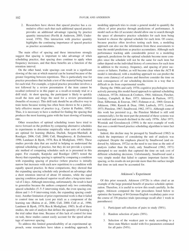
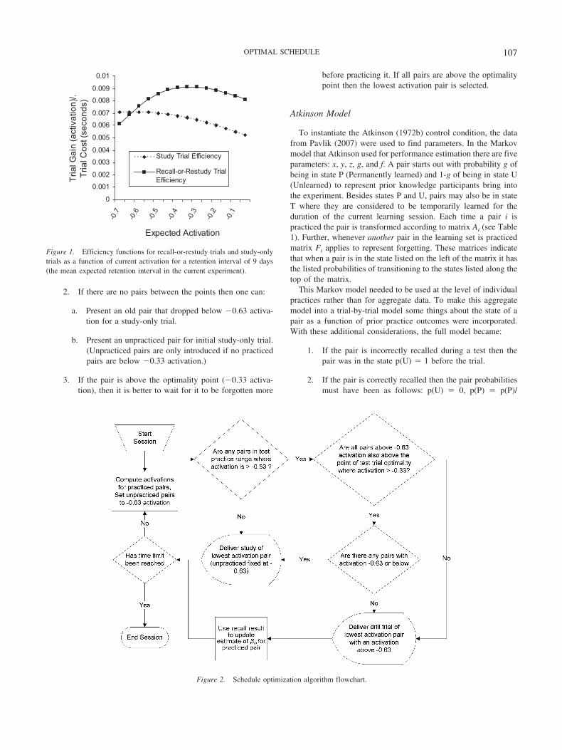
Determining optimality conditions. Using versions of Equa-tion 1 (see Equation 7 and Equation 8 in the Appendix), it waspossible to describe the practice efficiency functions for recall-or-restudy trials and study-only trials as a function of expectedactivation for the 9-day average retention interval in the experi-ment. See Figure 1, which shows our predictions that an expectedactivation of �0.33 was optimal for recall-or-restudy trials andthat when expected activation dropped to �0.63 it became moreadvantageous to give a study-only trial. Figure 2 shows this se-lection algorithm graphically.

1. If the pair is above the study advantage point (�0.63activation) but below the optimality point (�0.33 activa-tion), then the pair should be drilled (i.e., given a recall-or-restudy trial) because waiting longer will result in lessefficient practice. If multiple pairs are in the range, theweakest is chosen.


2. If there are no pairs between the points then one can:

a. Present an old pair that dropped below �0.63 activa-tion for a study-only trial.

b. Present an unpracticed pair for initial study-only trial.(Unpracticed pairs are only introduced if no practicedpairs are below �0.33 activation.)

3. If the pair is above the optimality point (�0.33 activa-tion), then it is better to wait for it to be forgotten more

before practicing it. If all pairs are above the optimalitypoint then the lowest activation pair is selected.

Atkinson Model

To instantiate the Atkinson (1972b) control condition, the datafrom Pavlik (2007) were used to find parameters. In the Markovmodel that Atkinson used for performance estimation there are fiveparameters: x, y, z, g, and f. A pair starts out with probability g ofbeing in state P (Permanently learned) and 1-g of being in state U(Unlearned) to represent prior knowledge participants bring intothe experiment. Besides states P and U, pairs may also be in stateT where they are considered to be temporarily learned for theduration of the current learning session. Each time a pair i ispracticed the pair is transformed according to matrix Ai (see Table1). Further, whenever another pair in the learning set is practicedmatrix Fi applies to represent forgetting. These matrices indicatethat when a pair is in the state listed on the left of the matrix it hasthe listed probabilities of transitioning to the states listed along thetop of the matrix.

This Markov model needed to be used at the level of individualpractices rather than for aggregate data. To make this aggregatemodel into a trial-by-trial model some things about the state of apair as a function of prior practice outcomes were incorporated.With these additional considerations, the full model became:

1. If the pair is incorrectly recalled during a test then thepair was in the state p(U) � 1 before the trial.

2. If the pair is correctly recalled then the pair probabilitiesmust have been as follows: p(U) � 0, p(P) � p(P)/

Figure 2. Schedule optimization algorithm flowchart.

0

0.001

0.002

0.003

0.004

0.005

0.006

0.007

0.008

0.009

0.01

-0.7

-0.6

-0.5

-0.4

-0.3

-0.2

-0.1

Expected Activation

Tria

l Ga

in (

activ

atio

n)/.

Tri

a l C

ost

(se

con

ds)

Study Trial Efficiency

Recall-or-Restudy TrialEfficiency

Figure 1. Efficiency functions for recall-or-restudy trials and study-onlytrials as a function of current activation for a retention interval of 9 days(the mean expected retention interval in the current experiment).

107OPTIMAL SCHEDULE

(p(P)�p(T)), and p(T) � p(T)/ (p(P)�p(T)) becausep(P)�p(T) must sum to 1 if the item was recalled.

3. After any trial of a pair, learning from the feedback studyor the correct retrieval lead to Ai being applied for thatpair

4. the Fimatrix is applied to all other pairs when any pair ispracticed.

5. When a pair survives a between-session retention intervalit has been permanently learned, p(P) � 1, p(T) � 0, andp(U) � 0. (This model component also means a pair willno longer receive practice if the first test following along-term retention interval succeeds.)

Table 2 shows the overall parameters determined for this modelfrom the (Pavlik, 2007) data. To decide which pair to practice,Atkinson (1972b) used the Markov model to compute the pair thatwould have the greatest chance to shift into the permanent state ifpracticed next. This is also how the algorithm worked here for thecontrol condition in this experiment; however, rather than intro-duce pairs with test-and-study trials as Atkinson did, the first trialfor each word pair in the Atkinson control condition was a studypresentation and subsequent presentations were recall-or-restudytrials. Further, because the schedule optimization in the 1972 paperused a minimum spacing of six intervening trials, the version herewas likewise constrained to a minimum spacing of six betweenrepetitions. However, pairs were not segregated into groups forrotation like Atkinson, rather, pairs were simply prevented frombeing selected if they had occurred in the last six trials and the nextbest pair was selected. (A bug affected 1.2% of trials, resulting inspacings shorter than six intervening trials.)

Results and Discussion

Figure 3 shows average performance for each session for eachof three dependent measures. The left panels show Sessions 1through 3 and the right panels provide Session 4 results with 95%confidence intervals. The main statistical question of interest waswhether the schedule optimization condition had an effect on thedependent measures of correctness and latency. The graphs showthat these effects were significant for Session 4 recall and latency,F(2, 57) � 5.4, p � .0073 and, F(2, 57) � 10.3, p � .00015, withall pairwise t test comparisons favoring the schedule optimization,

( ps � 0.05). For correctness, these results show a Cohen’s-d effectsize of 0.796 SD compared to the Atkinson control and 0.978 SDcompared to the flashcard control. For latency, these results showan effect size of 1.17 SD compared to the Atkinson control and1.31 SD compared to the flashcard control. Failure latency was notsignificantly affected by condition. Before running the experiment,we simulated the predicted probabilities of recall according to theACT-R model for the first trial of the assessment session for thethree conditions and showed a similar result. The simulated valueswere 56% for the optimization condition, 31% for the flashcardcondition, and 24% for the Atkinson condition. These are belowthe actual observed values 66%, 35%, and 40%, respectively. Thissuggests that, whereas the model was generally biased to under-estimate performance, it seems to well capture the advantage of theoptimized condition relative to the controls.

Recall that the design included different nested subconditionsets of pairs within each between-subjects condition. For thelearning rate optimization method condition, the utility of usingprior item � values was tested to see if they provided an enhance-ment to the schedule optimization. To do this, before the experi-ment began for each participant, half of the pairs with prior item �estimates were randomly designated to not use those estimates.This allowed a comparison of performance of the schedule opti-mization in conditions when the pairs had item �s and used themand when the pairs had item �s but did not use them. AlthoughSession 4 results showed no effect of whether item �s were used,there was a significant advantage for item �s during learning (F(1,19) � 5.4, p � .032, d � 0.377). This suggests that the item �s didhave some benefit because they caused a significant reduction inerrors during learning. However, because no effect carried throughto Session 4, we probably should conclude that prior item �s arenot very important to the overall goal of improving learning. Ofcourse, this result depends on the pairs we used as stimuli, since ifthere were less homogeneity of difficulty among the pairs, item �swould have been larger and had a stronger effect on practiceselection.

The results for the nested analysis performed in the flashcardcontrol condition showed no serious differences for the new wordsin the set. In this case, retention of pairs that were new to thelearning set (108 pairs) and the old learning set (100 pairs) wascompared. There was a 1.3% difference in Session 1 thru 4performance, which was statistically significant (F(1, 19) � 9.3,p � .0065, d � 0.0745). This difference reflected the fact that the108 new word pairs were very slightly easier than the prior set of100 word pairs. Although this difference was significant, therewere no interactions and the effect size was very small, so it isimplausible to suppose that the new words could have confoundedthe results of this experiment.

Table 1Atkinson (1972b) Markov Model

Initial state

Final state Permanent Temporary Unlearned

Learning matrix (Ai)Permanent 1 0 0Temporary xi 1-xi 0Unlearned yi zi 1-yi-zi

Forgetting matrix (Fi)Permanent 1 0 0Temporary 0 1-fi fiUnlearned 0 0 1

Table 2Overall Atkinson (1972b) Parameters for Pavlik (2007) Data

Parameter Value

x 0.18y 0.21z 0.59g 0f 0.011


Figure 4 shows the results of the nested analysis performed inthe Atkinson (1972b) control condition. For this analysis, perfor-mance on five overall parameter pairs was compared with thosepairs for which five individual parameters had been found. Thegraph shows a somewhat different pattern than expected. Based onAtkinson, one might have expected worse initial performance andbetter final performance for the individual parameter words. How-ever, this did not occur because of the way the Atkinson routine

chose to introduce the overall parameter pairs as a cohort. This isillustrated by examining what happens to a pair responded toincorrectly in either the overall or the individual conditions. In theoverall condition all pairs come up for practice at the same time,if they are responded to incorrectly, they must be in the U state andthen have practice matrix Ai applied. This leaves the probabilitiesequal again, and the pairs will therefore come up for practice againat the same time (after the whole cohort of overall parameter failed

Session

321

Pro

babi

lity

Cor

rect

1.0

.8

.6

.4

.2

Condition

Optimization

Flashcard

Atkinson (1972b)0

0.10.20.30.40.50.60.70.80.9

Optimization Flashcard Atkinson (1972b)

Prob

ability Correc t

a) Session 1-3 : recall probability b) Session 4: recall probability

Session

321

Mea

n La

tenc

y (m

s)

2800.0

2600.0

2400.0

2200.0

2000.0

1800.0

1600.0

1400.0

Condition

Optimization

Flashcard

Atkinson (1972b)

c) Session 1-3 : recall latency d) Session 4: recall latency

Session

321

Fai

lure

Lat

ency

(m

s)

5000.0

4500.0

4000.0

3500.0

3000.0

2500.0

Condition

Optimization

Flashcard

Atkinson (1972b)0

500100015002000250030003500400045005000

Optimization Flashcard Atkinson (1972b)

Failu

r e Laten

c y (m

s)

e) Session 1-3 : failure latency f) Session 4: failure latency

Figure 3. Main results for learning and performance.

109OPTIMAL SCHEDULE

pairs has cycled). In contrast, when an individual parameter pairhas the highest transition probability to state P, and is then incor-rectly responded to on the scheduled test, it will come up again atabout the minimum spacing.

The results of the between-subjects overall difficulty subcondi-tion were analyzed to determine what influence the three condi-tions might have had on pairs not being scheduled by the algo-rithms. The mean recall levels for all tests on these pairs was0.567, 0.435, and 0.489 for the schedule optimization, flashcard,and Atkinson conditions, respectively. A first repeated measuresANOVA looked for significant difference because of condition.Although this overall ANOVA confirmed that differences exist,F(2, 57) � 4.3, p � .019, follow-up t tests showed that only thedifference between the optimization and the flashcard conditionswas significant ( p � .0052, d � 0.922). However, a trend wasobserved for the optimization-Atkinson comparison ( p � .094). Asecond ANOVA looked only at first session tests where recallprobability during learning was maximally different, since the

greatest differences might be expected during this session. Indeed,the comparison was significant, F(2, 57) � 5.3, p � .0075 withpairwise t test comparisons significant for the flashcard conditioncomparison ( p � .016, d � 0.794) and the Atkinson conditioncomparison ( p � .0032, d � 0.978).

Modeling Questions

It is also possible to use the data from the human participants toask questions about the models used to optimize performance.

Predictive validity of the ACT-R model during learning. Oneinteresting question is how well the ACT-R model can predictrecall given data about learning. To answer this question aboutprediction, it was possible to use the model with the prior overallparameters from Table 3 and the individual difference parameters(�s) determined during the three learning sessions from the Bayes-ian procedure described at the end of the Appendix. For eachoptimization condition participant, Session 4 Trial 1 probability ofrecall prediction was compared to the actual value the participantproduced to determine the deviation of the model from the partic-ipant. Predictions for the 20 participants had an r2 value of 0.86with a mean absolute deviation of 0.9% (SD 9.6%).

Testing the Atkinson model long-term memory assumption. Aswas discussed earlier, one assumption of the Atkinson (1972b)model was that pairs in the permanently learned state cannot beforgotten. Because pairs are further assumed to lose all temporarystrength during a long-term interval, an initial correct recall after along-term interval necessarily implies a pair is in the permanentstate with a probability of 1. Thus, pairs that are successfullyrecalled on the first opportunity after the long-term interval are nolonger selected for practice by the algorithm.

This assumption of permanent memory seemed implausible, butit was possible to look at the data in the Atkinson condition to seehow often these abandoned pairs were recalled during the assess-ment session. To do this the average assessment session recall wascomputed for the first trial of the assessment session for any pairsthat were abandoned for further practice after being responded to

Session4321

Pro

babi

lity

Cor

rect

.80

.70

.60

.50

.40

.30

.20

.10

Item type condition

Overall items

Individual items

Figure 4. Five parameter overall compared to five parameter per pairsubcondition results for the Atkinson (1972b) model condition.

Table 3Parameter Values and Usage

Parameter type Symbol ValueUsed in

simulationUsed to compute

criteriaUsed duringoptimization

Activation a 0.177 Yes Yes Yesc 0.279 Yes Yes Yesh 0.0172 Yes Yes Yes

Recall � -0.704 Yes Yes Nos 0.0786 Yes Yes No

Latency F 1.29 Yes Yes Nos2 0.75 Yes Yes No

Study u 1.205 No Yes Nov 0.000598 No Yes No

Fixed costs Failure cost 8.2s Yes Yes NoSuccess cost 2.4s Yes Yes NoStudy cost 4.5s No Yes No

� participant �s SD�0.283 Yes No No� item �i varied Yes No Yes� participant/item �si SD�0.50 Yes No YesDifficulty Slope 1.45 Yes Yes Yes

Intercept 0.961 Yes Yes Yes


correctly for their first recall-or-restudy trial on either Session 2 or3. The average probability of first trial assessment session recallfor these pairs was 0.57 (SD � 0.26). This clearly indicates that theassumption of a “permanent” memory state fits the data poorly.

Again, though this reveals a weakness in the Atkinson model’sfit, the model might be corrected to overcome this problem with itsaccuracy by simple increasing the number of states the memorycould be in beyond just Unlearned, Temporary, and Permanent.For example, by splitting the Permanent state into two states(Long-term and Permanent) the model could be made to captureforgetting between sessions in an analogous manner as it currentlycaptures forgetting between trials (by using a forgetting parameterthat allows for only some items to become unlearned when there isanother item tested). Of course, this revised model would havemore complexity and parameters, but the feasibility of such fourstage models has been shown in prior research (Atkinson &Crothers, 1964).

General Discussion

Ever since Ebbinghaus’ (1913/1885) discovery of the spacingeffect, researchers have considered how to best make use of thisprinciple to improve how people learned. Although it is clear thatsome spacing of practice is almost always good, despite more thana century of research the jury appears to still be out on how muchspacing is best (e.g., contrast this paper with Pashler et al., 2003).To resolve this longstanding theoretical debate, this paper em-ployed an economic analysis instantiated by a computationalmodel to compute the optimal schedule of practice for each item.

Theoretical Implications

Our results are theoretically important because they stronglyqualify the proposition that wider spacing is typically the bestpractice (Atkinson, 1972b; Bahrick, 1979; Karpicke & Roediger,2007; Pashler et al., 2003; Schmidt & Bjork, 1992). Our experi-ment and theoretical analysis shows that by sacrificing wide spac-ing benefits we can take advantage of recency effects and savetime and thus provide significantly more practice. Figure 5 showsthe significant effect of condition on the number of trials for theoverall comparison (F(2, 57 � 12.5, p � .000032) with pairedcomparisons with the optimization method condition significantfor both the flashcard ( p � .0000062, d � 2.21) and Atkinson( p � .0060, d � 0.807) control conditions.

Our results are different and in conflict with current theorybecause our theory of spacing effect efficiency acknowledges thattime costs per trial for spaced practice can easily grow faster thanbenefits per trial as spacing increases past a certain point. Thetheory captures this by saying that wide spacing leads to lessforgetting, but also results in longer trial latencies. Given a specificretention interval, the modeling method that implements the theoryallows one to compute the optimal spacing that maximizes thisreduction in forgetting relative to the longer trial durations. Themethod suggests that initial spacing should be very short becausethe model predicted 99.2% recall during learning as optimal for thetask here (in the minimum noise case). Although this prediction ofhigh level of recall during learning is in general agreement withSkinner (1968) and his theory that errorless learning is optimal,unlike Skinner, the current research provided a mechanistic expla-

nation for why this should be so by appealing to cognitive con-structs (e.g., the strength of a declarative memory), something thatSkinner was unwilling to do. Further, this research provided awell-controlled experimental test of the notion that error minimi-zation results in better learning.

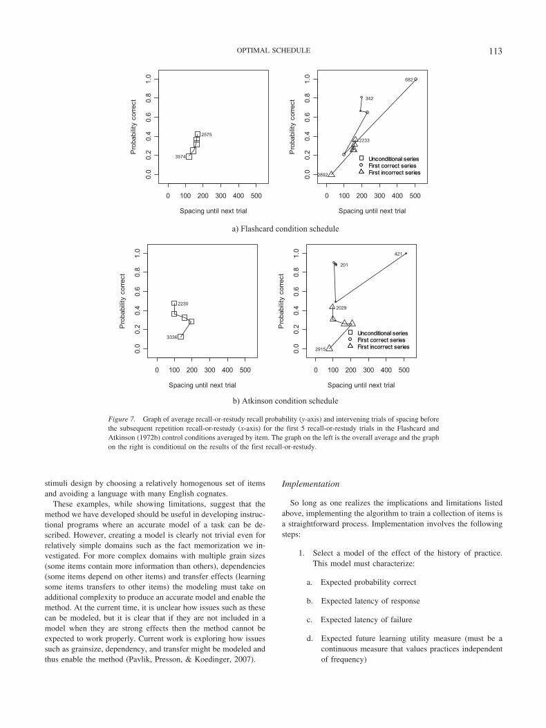
Figures 6 and 7 show one way to visualize the data collectedduring learning. Because the vast majority of trials for each userwere recall-or-restudy practice, the graphs plot correctness andspacing for recall-or-restudy trials only. The y-axes capture thecorrectness (averaged across items) for each of the first fiverecall-or-restudy trials, whereas the x-axes captures the spacingfollowing each of these trials. To read the graphs, note that for eachpanel the first trial of each series is labeled with the count ofobservations, as is the last trial. This gives a perspective on thequantity of practice for each item in the various conditions. Inaddition, note that the left sides of Figures 6 and 7 show the overallaverage, whereas the right sides show performance conditional onthe results of the first recall-or-restudy. These condition graphsshow that there is a tendency in all conditions to schedule morerepetitions when the first repetition is responded to incorrectly. Wecan see on the right side of Figure 6 that the optimization methodreacts to correctness by increasing the spacing of the schedule andincorrectness by decreasing the spacing of the schedule and thataverage correctness is maintained at a relatively high and constantlevel in both cases. In contrast, the control conditions show adifferent pattern that gives much wider spacing after a correctanswer, but which subsequently contracts to become narrowerbecause second trial failures are very high.

The smoothly expanding spacing of practice produced by themethod is in general agreement with the theory that expandingspacing of practice may be optimal (Cull et al., 1996; Landauer &Bjork, 1978; Rea & Modigliani, 1985). However, although these

Atkinson(1972b)

Flashcard

Optimization

Dril

l Tria

ls D

urin

g Le

arni

ng S

essi

ons 2400

2200

2000

1800

1600

1400

1200

Figure 5. Total recall-or-restudy trials during learning by condition (95%CI error bars).

111OPTIMAL SCHEDULE

studies only support expanding spacing for a test-only procedure(no review following errors), by attending to the costs of widerspacing our method has demonstrated that expanding spacing mayalso be optimal for recall-or-restudy trials. The method producesthis expanding spacing because of the effect of frequency in theACT-R model. As frequency increases, an item becomes morestable in memory because the model implements power functionforgetting which results in strength from older accumulated prac-tices decaying increasingly slowly as time passes. This increasedstability with increased frequency allows more time betweenspaced practices as repetitions accumulate. Thus, our modelingapproach has allowed us to derive that expanding spacing is theoptimal solution to the scheduling problem by quantifying thetheoretical relationships between recency, frequency, and spacingand their effects on final performance.

Practical Implications

Although the method clearly has implications for the learning oflarge sets of paired-associate items by young naı̈ve participants, itis less obvious what this implies for different tasks, differentpopulations of learners, or different materials. Take for example adifferent task like recognition. The interesting difference aboutrecognition tasks is that there is no need for review in the case ofan error because the presentation of the test probe itself can serveas the learning necessary for later judgments of recognition. Be-cause there is therefore no need for review study opportunities, thecost of errors is much less. Therefore, because correctness wouldno longer be so important, recency would no longer provide anadvantage and the peak learning rate spacing interval would bemuch longer than in our experiment here. In fact, unless there wereother costs to consider, the method would probably suggest max-imal even spacing of practice as optimal unless the set of itemswere extremely large.

It is similarly straightforward to speculate about other learningsituations that may be amenable to the method we have described.Because procedural tasks are typically represented as if-then rulesthat might be collected into a set of items and trained using drillpractice, they also seem applicable to the method here assuming an

accurate model could be found. Prior work on procedural learning(e.g., Carlson & Yaure, 1990; Mayfield & Chase, 2002) hascompared blocked practice (a form of massed practice) versusmixed practice (which requires wider spacing of practice) andfound that mixed presentation schedules caused an advantage toretention. These results are important because they provide evi-dence that rule-based items may behave according to a sort ofspacing effect (any advantage to retention when using more dis-tributed practice). Since the optimization method harnesses spac-ing effects in deciding practice schedules, knowing that the spac-ing effect applies to practice of rule application skills is important.Further, we can note that procedural tasks often have high failurecosts. Together, these facts imply that procedural tasks may havean optimal expanding schedule similar to the one produced in theexperiment here. However, because parameter values such as theforgetting rate (which controls the effect of recency) and theamount of learning per repetition might differ greatly, the magni-tude of the spacing intervals might differ greatly.

The age of participants would also be likely to alter the optimalschedule. For instance, research by Balota et al. (1989, 2006)shows that although there tends to be no interaction of age andspacing effect, older individuals have generally worse recall. Thisrecall deficit might be modeled as an increase in forgetting or areduction in learning. Changes in the model parameters controllingthese effects would tend to result in less wide practice schedulesbecause narrower schedules would produce higher levels of recallduring learning (and thus avoid costly review opportunities). How-ever, the issue is complex because the schedule changes woulddepend upon which parameter(s) was used to capture the agerelated differences. For example, if deficient performance iscaused by a higher level of memory strength variability, capturedby the noise (s) parameter in the ACT-R model, the model’sprecision of recall probability prediction would decrease and thebenefit of spacing would dominate the learning rate equation. Thiswould imply wider spacing, or, in the case of very high noise, themodel would predict maximal spacing at all times. This possibilityis one reason why we tried to reduce overall variability during

0 50 100 150 200

0.0

0.2

0.4

0.6

0.8

1.0

Spacing until next trial

Pro

babi

lity

corr

ect 3115

2720

0 50 100 150 200

0.0

0.2

0.4

0 .6

0.8

1.0


Pro

babi

lity

corr

ect

2290

1916

Unconditional seriesFirst correct seriesFirst incorrect series825

804

Unconditional seriesFirst correct seriesFirst incorrect series

Figure 6. Graph of average recall-or-restudy recall probability (y-axis) and intervening trials of spacing beforethe subsequent repetition recall-or-restudy (x-axis) for the first 5 recall-or-restudy trials in the optimizationmethod condition. The graph on the left is the overall average and the graph on the right is conditional on theresults of the first recall-or-restudy.


stimuli design by choosing a relatively homogenous set of itemsand avoiding a language with many English cognates.

These examples, while showing limitations, suggest that themethod we have developed should be useful in developing instruc-tional programs where an accurate model of a task can be de-scribed. However, creating a model is clearly not trivial even forrelatively simple domains such as the fact memorization we in-vestigated. For more complex domains with multiple grain sizes(some items contain more information than others), dependencies(some items depend on other items) and transfer effects (learningsome items transfers to other items) the modeling must take onadditional complexity to produce an accurate model and enable themethod. At the current time, it is unclear how issues such as thesecan be modeled, but it is clear that if they are not included in amodel when they are strong effects then the method cannot beexpected to work properly. Current work is exploring how issuessuch as grainsize, dependency, and transfer might be modeled andthus enable the method (Pavlik, Presson, & Koedinger, 2007).

Implementation

So long as one realizes the implications and limitations listedabove, implementing the algorithm to train a collection of items isa straightforward process. Implementation involves the followingsteps:

1. Select a model of the effect of the history of practice.This model must characterize:

a. Expected probability correct

b. Expected latency of response

c. Expected latency of failure

d. Expected future learning utility measure (must be acontinuous measure that values practices independentof frequency)

0 100 200 300 400 500

0.0

0.2

0.4

0.6

0.8

1.0


Pro

babi

lity

corr

ect

3574

2575

0 100 200 300 400 500

0.0

0.2

0.4

0.6

0.8

1.0


Pro

babi

lity

c orr

e ct

682

342


2233


a) Flashcard condition schedule

0 100 200 300 400 500

0.0

0.2

0.4

0.6

0.8

1.0


Pro

babi

lity

corr

ect

3336

2230

0 100 200 300 400 500

0.0

0.2

0.4

0 .6

0 .8

1 .0


Pro

babi

lity

cor r

ect

421

201


2029


b) Atkinson condition schedule

Figure 7. Graph of average recall-or-restudy recall probability (y-axis) and intervening trials of spacing beforethe subsequent repetition recall-or-restudy (x-axis) for the first 5 recall-or-restudy trials in the Flashcard andAtkinson (1972b) control conditions averaged by item. The graph on the left is the overall average and the graphon the right is conditional on the results of the first recall-or-restudy.

113OPTIMAL SCHEDULE

2. Estimate the model’s parameters (using prior data)

3. Use the model before each drill trial to compute for everyitem:

a. Expected learning rate � (expected future learningutility gain for a practice/expected time cost for apractice)

b. Choose each item for practice at its maximum ex-pected learning rate

c. Repeat until stopping criterion for time practiced orexpected performance

References

Anderson, J. R., Fincham, J. M., & Douglass, S. (1997). The role ofexamples and rules in the acquisition of a cognitive skill. Journal ofExperimental Psychology: Learning, Memory, and Cognition, 23, 932–945.

Anderson, J. R., & Lebiere, C. (1998). The atomic components of thought.Mahwah, NJ: Erlbaum Publishers.

Anderson, J. R., & Schooler, L. J. (1991). Reflections of the environmentin memory. Psychological Science, 2, 396–408.

Atkinson, R. C. (1972a). Ingredients for a theory of instruction. AmericanPsychologist, 27, 921–931.

Atkinson, R. C. (1972b). Optimizing the learning of a second-languagevocabulary. Journal of Experimental Psychology, 96, 124–129.

Atkinson, R. C. (1975). Mnemotechnics in second-language learning.American Psychologist, 30, 821–828.

Atkinson, R. C., & Crothers, E. J. (1964). A comparison of paired-associatelearning models having different acquisition and retention axioms. Jour-nal of Mathematical Psychology, 1, 285–315.

Atkinson, R. C., Fletcher, D., Lindsay, J., Campbell, J. O., & Barr, A.(1973). Computer assisted instruction in initial reading: Individualizedinstruction based on optimization procedures. Educational Technology,8, 27–37.

Atkinson, R. C., & Paulson, J. A. (1972). An approach to the psychologyof instruction. Psychological Bulletin, 78, 49–61.

Bahrick, H. P. (1979). Maintenance of knowledge: Questions about mem-ory we forgot to ask. Journal of Experimental Psychology: General, 108,296–308.

Balota, D. A., Duchek, J. M., & Paullin, R. (1989). Age-related differencesin the impact of spacing, lag, and retention interval. Psychology andAging, 4, 3–9.

Balota, D. A., Duchek, J. M., Sergent-Marshall, S. D., & Roediger, H. L.,III (2006). Does expanded retrieval produce benefits over equal-intervalspacing? Explorations of spacing effects in healthy aging and early stageAlzheimer’s disease. Psychology and Aging, 21, 19–31.

Carlson, R. A., & Yaure, R. G. (1990). Practice schedules and the use ofcomponent skills in problem solving. Journal of Experimental Psychol-ogy: Learning, Memory, and Cognition, 16, 484–496.

Carrier, M., & Pashler, H. (1992). The influence of retrieval on retention.Memory & Cognition, 20, 633–642.

Coltheart, M. (1981). The MRC psycholinguistic database. Quarterly Jour-nal of Experimental Psychology: Human Experimental Psychology, 33,497–505.

Cull, W. L. (2000). Untangling the benefits of multiple study opportunitiesand repeated testing for cued recall. Applied Cognitive Psychology, 14,215–235.

Cull, W. L., Shaughnessy, J. J., & Zechmeister, E. B. (1996). Expandingunderstanding of the expanding-pattern-of-retrieval mnemonic: Toward

confidence in applicability. Journal of Experimental Psychology: Ap-plied, 2, 365–378.

Dear, R. E., Silberman, H. F., & Estavan, D. P. (1967). An optimal strategyfor the presentation of paired-associate items. Behavioral Science, 12,1–13.

Dempster, F. N. (1996). Distributing and managing the conditions ofencoding and practice. In R. A. Bjork & E. L. Bjork (Eds.), Memory (pp.317–344). New York: Academic Press.

Ebbinghaus, H. (1913). Memory: A contribution to experimental psychol-ogy (translated by Henry A. Ruger & Clara E. Bussenius; originalGerman work published 1885). New York: Teachers College, ColumbiaUniversity.

Fishman, E. J., Keller, L., & Atkinson, R. C. (1969). Massed versusdistributed practice in computerized spelling drills. In R. Atkinson &H. A. Wilson (Eds.), Computer assisted instruction. New York: Aca-demic Press.

Glenberg, A. M. (1976). Monotonic and nonmonotonic lag effects inpaired-associate and recognition memory paradigms. Journal of VerbalLearning & Verbal Behavior, 15, 1–16.

Groen, G. J., & Atkinson, R. C. (1966). Models for optimizing the learningprocess. Psychological Bulletin, 66, 309–320.

Karpicke, J. D., & Roediger, H. L., III. (2007). Expanding retrieval practicepromotes short-term retention, but equally spaced retrieval enhanceslong-term retention. Journal of Experimental Psychology: Learning,Memory, and Cognition, 33, 704–719.

Karush, W., & Dear, R. E. (1966). Optimal stimulus presentation strategyfor a stimulus sampling model of learning. Journal of MathematicalPsychology, 3, 19–47.

Landauer, T. K., & Bjork, R. A. (1978). Optimum rehearsal patterns andname learning. In M. M. Gruneberg, P. E. Morris, & R. N. Sykes (Eds.),Practical aspects of memory (pp. 625–632). New York: AcademicPress.

Laubsch, J. H. (1971). An adaptive teaching system for optimal itemallocation. Dissertation Abstracts International, 31, 3961.

Lorton, P. V. (1973). Computer-based instruction in spelling: An investi-gation of optimal strategies for presenting instructional material. Dis-sertation Abstracts International, 34, 3147.

Mayfield, K. H., & Chase, P. N. (2002). The effects of cumulative practiceon mathematics problem solving. Journal of Applied Behavior Analysis,35, 105–123.

Metcalfe, J., & Kornell, N. (2003). The dynamics of learning and allocationof study time to a region of proximal learning. Journal of ExperimentalPsychology: General, 132, 530–542.

Murphy, G., & Kovach, J. (1972). Historical introduction to modernpsychology. New York: Harcourt Brace Jovanovich.

Nelson, T. O., & Leonesio, R. J. (1988). Allocation of self-paced studytime and the “labor-in-vain effect.” Journal of Experimental Psychol-ogy: Learning, Memory, and Cognition, 14, 676–686.

Pashler, H., Cepeda, N. J., Wixted, J. T., & Rohrer, D. (2005). When doesfeedback facilitate learning of words? Journal of Experimental Psychol-ogy: Learning, Memory, and Cognition, 31, 3–8.

Pashler, H., Zarow, G., & Triplett, B. (2003). Is temporal spacing of testshelpful even when it inflates error rates? Journal of ExperimentalPsychology: Learning, Memory, and Cognition, 29, 1051–1057.

Pavlik, P. I., Jr. (2005). The microeconomics of learning: Optimizingpaired-associate memory. Dissertation Abstracts International: SectionB: The Sciences and Engineering, 66, 5704.

Pavlik, P. I., Jr. (2006). Understanding and applying the dynamics of testpractice and study practice [Electronic Version]. Instructional Science,from http://dx.doi.org/10.1007/s11251–006–9013–2.

Pavlik, P. I., Jr. (2007). Timing is an order: Modeling order effects in thelearning of information. In F. E., Ritter, J. Nerb, E. Lehtinen, & T. O’Shea(Eds.), In order to learn: How order effects in machine learning illuminatehuman learning (pp. 137–150). New York: Oxford University Press.


Pavlik, P. I., Jr., & Anderson, J. R. (2005). Practice and forgetting effectson vocabulary memory: An activation-based model of the spacing effect.Cognitive Science, 29, 559–586.

Pavlik, P. I., Jr., Presson, N., & Koedinger, K. R. (2007). Optimizingknowledge component learning using a dynamic structural model ofpractice. In R. Lewis & T. Polk (Eds.), Proceedings of the EighthInternational Conference of Cognitive Modeling. Ann Arbor: Universityof Michigan.

Peterson, L. R., Wampler, R., Kirkpatrick, M., & Saltzman, D. (1963).Effect of spacing presentations on retention of a paired associate overshort intervals. Journal of Experimental Psychology, 66, 206–209.

Pimsleur, P. (1967). A memory schedule. The Modern Language Journal,51, 73–75.

Rea, C. P., & Modigliani, V. (1985). The effect of expanded versus massedpractice on the retention of multiplication facts and spelling lists. HumanLearning: Journal of Practical Research & Applications, 4, 11–18.

Ruch, T. C. (1928). Factors influencing the relative economy of massedand distributed practice in learning. Psychological Review, 35, 19–45.

Schmidt, R. A., & Bjork, R. A. (1992). New conceptualizations of practice:

Common principles in three paradigms suggest new concepts for train-ing. Psychological Science, 3, 207–217.

Skinner, B. F. (1968). The technology of teaching. East Norwalk, CT:Appleton-Century-Crofts.

Smallwood, R. D. (1962). A decision structure for teaching machines.Cambridge: MIT Press.

Smallwood, R. D. (1971). The analysis of economic teaching strategies for asimple learning model. Journal of Mathematical Psychology, 8, 285–301.

Thios, S. J., & D’Agostino, P. R. (1976). Effects of repetition as a functionof study-phase retrieval. Journal of Verbal Learning & Verbal Behavior,15, 529–536.

Underwood, B. J. (1970). A breakdown of the total-time law in free-recalllearning. Journal of Verbal Learning & Verbal Behavior, 9, 573–580.

Underwood, B. J., Kapelak, S. M., & Malmi, R. A. (1976). The spacingeffect: Additions to the theoretical and empirical puzzles. Memory &Cognition, 4, 391–400.

Wozniak, P. A., & Gorzelanczyk, E. J. (1994). Optimization of repetitionspacing in the practice of learning. Acta Neurobiologiae Experimentalis,54, 59–62.

Appendix: ACT-R Model

Activation Equation (Memory Strength Function). Practiceeffects and item/individual differences are captured by an ac-tivation equation (Equation 2), which represents the strength ofan item in memory as the sum of the remaining learning froma number of individual memory strengthenings and valuesrepresenting the item/individual differences. Each strengthen-ing corresponds to a past practice event (either a memoryretrieval or study event). Specifically, Equation 2 proposes thateach time an item is practiced, the activation of the item, mn

(activation on the nth practice) receives a boost in strength thatdecays away as a power function of time. Each tk in Equation2 equals the age of trial k, whereas each dk equals the decay ratefor trial k. The � parameters are a new addition (Pavlik, 2007).They capture any deviation of the overall model from the datafor any particular sequence of tests with an item for a partici-pant. They represent differences at the level of the item (�i),participant (�s), and participant/item (�si).

mn(t1..n) � �s � �i � �si � ln� �k � 1

n

tk�dk� (2)

To deal with the spacing effect Equation 3 was developed to estimatedecay for the kth trial, dk, as a function of the activation at the time itoccurred. The implication of this function is that higher activation atthe time of a practice will result in the benefit of that practice decayingmore quickly. On the other hand, if activation is low, decay willproceed more slowly. It is important to note that every practice has itsown dk that controls the forgetting of that practice. In Equation 3 thedecay rate dk is calculated for the kth presentation of an item as afunction of the activation mk-1at the time the presentation occurred(e.g., the decay rate for the 7th trial (t7) depends on the activation at the

time of the seventh trial, which is a function of the prior six trials’ agesand decay rates. It is important to note that since tks are ages,activation and decay depend on the current time as well as the numberof practices).

dk(mk � 1) � cemk � 1 � � (3)

In Equation 3, c is the decay scale parameter, and a is the interceptof the decay function. For the first practice of any sequence, d1 �a because m0 is equal to negative infinity. These equations arerecursive because to calculate any particular mn at the time of trialn, one must have previously calculated the dk needed for each ofthe prior n-1 trials, which requires knowing the prior mns.

These equations result in a steady decrease in the long-runretention for more presentations in a sequence where presentationsare closely spaced. As spacing gets wider in such a sequence,activation has time to decrease between presentations, decay istherefore lower for new presentations and long-run retention ef-fects do not decrease as much.

Individual and Item Differences and �

The use of � to represent constant noise has been implicit in thesystem since at least Anderson and Lebiere (1998). In that docu-mentation of the declarative memory system two sources of thenoise are proposed. These two types of noise are referred to aspermanent activation noise and temporary activation noise. Per-manent activation noise is exactly equivalent to the sum of thethree � components. In contrast, random trial-to-trial noise iscaptured in the s parameter in Equation 4 below, which representsthe probability of recall given a random logistic distribution ofactivation (with s controlling the variance).

(Appendix continues)

115OPTIMAL SCHEDULE

Recall Equation

In ACT-R, an item will be retrieved if its activation is above athreshold. Because activation is noisy, an item with activation m asgiven by Equation 4 has only a certain probability of recall.ACT-R assumes a logistic distribution of activation noise, in whichcase the probability of recall is:

p(m) �1

1 � e� � m

s

(4)

In Equation 4, � is the threshold parameter. As discussed, the sparameter controls the noise in activation and it describes thesensitivity of recall to changes in activation.

Retrieval Time Equation

The time to retrieve in ACT-R is shown in Equation 5. InEquation 5, F is the parameter that scales the effect of latency onactivation. Fixed time cost refers to the fixed time cost of percep-tual motor encoding and response.

l(m) � Fe�m � fixed time cost (5)

Intersession Forgetting in the Model

Anderson, Fincham, and Douglass (1997) found that althoughEquation 2 could account for practice and forgetting during anexperiment, it could not fit retention data over long intervals.Because of this, they supposed that between sessions, interveningevents erode memories more slowly than during an experimentalsession. This slower forgetting was modeled by scaling time as ifit was slower outside the experiment. Forgetting is therefore de-pendent on the “psychological time” between presentations ratherthan the real time. This psychological time factor is implementedby multiplying the portion of time that occurs between sessions bythe h parameter when calculating recall. This is done by subtract-ing h*total intersession time from each age (tk) in Equation 1.Because of this mechanism, time in the model is essentially ameasure of destructive interfering events. The decay rate, there-fore, is a measure of fragility of memories to the corrosive effectof these other events.

Study Duration Model

Because it was shown in Pavlik Jr. (2006) that ACT-Rsassumptions about study practice and test practice having equalmemorial consequences did not fit the data, and that a newmodel of study duration resulted in interesting predictions aboutefficiency, this new, better fitting model was used for thecurrent study. In this model strength of a study practice, b � u(1-e (duration-study trial fixed cost) � (-v)/number of items in the stimulus),where u is the maximum benefit of study and v describes therate of approach to the maximum. This simple model capturesthe fact that study practice has diminishing marginal returns andappears to reach an asymptotic level of encoding given a longenough encoding interval (Metcalfe & Kornell, 2003; Nelson &Leonesio, 1988). The study value is used as a factor for the termrepresenting the respective study learning events in the activa-

tion equation (Equation 6). In the case of test practices b isfixed at 1.

mn(t1..n) � �s � �i � �si � In� �k�1

n

bk tk�dk� (6)

Further, this study effect model had an additional component thatwas found to be useful in capturing the fact that study following afailed retrieval appeared to be more effective than study practicealone. To capture this effect of study after failure, the v parameterwas divided by the number of terms in the stimulus. This compo-nent of the model says that during study trials participants deployan attentional resource (typically in a strategic fashion, but alsothrough rote processes) to encode the stimulus being studied.Because this resource is limited, it must be divided among thecomponents of the stimulus (this is done in the model by dividingthe encoding rate by the stimulus size.) This limited-resourcemechanism implies that the advantage of a study after a failed testcomes from the opportunity to pre-encode the cue. Because of thispre-encoding of the prompt during the failed test study opportu-nity, the encoding of the single response term proceeds twice asquickly compared to a study-only trial.

Parameter Determination

The details of how parameters for these models were deter-mined, using data from Pavlik (2006) and Pavlik (2007), havebeen omitted, but are available on request from the author.Table 3 shows the final parameters used by the model in theschedule optimization or simulation. The right hand side ofTable 3 details that parameters were used to simulate theexperiment (simulation was completed before running the ex-periment), which parameters were used to determine the deci-sion criteria the schedule optimization algorithm would use(again, before the experiment), and which parameters were usedto predict memory strengths for the application of the decisioncriteria (during the experiment).

Determining Optimality Conditions

Given the ACT-R model, it was possible to compute the averageactivation gain after a 9-day retention interval (the average for theexperiment being optimized) for both recall-or-restudy trials andstudy-only trials as a function of different levels of activation.[One might have considered calculating this value for each day ofthe experiment separately, using 11, 9, and 7 days for each of thethree learning sessions, but the predictions vary little for theserelative small differences in retention so the average was used.]Given a set of parameter values, average activation gain for apractice depends on the activation (m) at the time of practice andthe duration of the retention interval (r). Similarly, one can com-pute the estimated time cost for both study-only trials and recall-or-restudy trials, including fixed costs of intertrial times. Again,the cost is a function of activation. These values were used tocompute the functions describing the activation gain per second forselecting a recall-or-restudy trial or selecting a study-only trial.

Equation 7 describes the activation gain per second of practicefor recall-or-restudy trials.


gain testn�r, mn

�p �mnr��cem� �a � �1 � p�mn � 95 � r��cem� �a

p�mn �Fe�m � fixed success cost� �1 � p�mn �fixed failure cost

(7)

In this equation, p is the probability of recall, r is the retentioninterval, and the other parameters are defined in Equation 2 andEquation 5. For simplicity, Equation 7 ignores the influence of thenatural logarithm in the activation equation (Equation 2). This wasfound to have an insignificant effect on predictions. Equation 7uses a 0.95 (b parameter) weight to capture the average effect ofthe 3-s feedback study after failed tests (see Equation 6).

Equation 8 describes the activation gain per second of practicefor study-only trials.

gain studyn(r, mn) �.79 � r��cem� � a

fixed study cost(8)

Equation 8 uses a 0.79 weight to capture the effect of a 4-s studydelivered alone (see Equation 6).

Correcting for Overall Difficulty

As the data showed here, there is also an effect of the context ofdifficulty. Because this effect was not captured in the model, butalso appeared to be present in the data from Pavlik (2007) acorrection was made to the model to capture this variance. For thiscorrection, the model assumed an additional � correction compo-nent that was a linear function of correctness during learning. Thiswas implemented by a linear model describing how overall diffi-culty during learning mapped to � during learning. This line wasthe equation � correction � average activation during learning *1.45 � 0.916. This correction was meant merely to capture vari-ance, and it seems that more data and theoretical work are neededto explain the phenomenon as discussed in the introduction. Thecorrection was applied when determining the values �0.66 and�0.33 from Equations 6 and 7 and was used when computingFigure 1. Further, this correction was applied to computing acti-vations during learning. During learning, the current correctionwas estimated after each trial for each participant by using the

inverse of Equation 3 and the overall average prior probability ofrecall for that participant to compute the average activation duringlearning.

Like Pavlik (2007), the algorithm was implemented with arequirement for a spacing of two trials between repetitions becauseit seemed risky to assume the model would be effective at veryshort intervals. It seemed possible that some sort of study-phaseretrieval spacing effect mechanism would severely block encodingat very short lags (a mechanism discussed by Thios & D’Agostino,1976). The algorithm had an interesting adaptation to this stricturebecause the average pair dropped below �0.63 activation after twointervening trials. For this reason, the schedule optimization beganby introducing most new pairs with two study-only trials, spaceddepending on the activations of other pairs. After the second studyaverage pairs were within the testing range (greater than �0.63activation) and received recall-or-restudy trials. Interestingly, be-cause the program updated an estimate of the participant � valueevery 300 trials, the number of introductory study-only trialsvaried and could go as high as 4 or 5 for very slow learningparticipants and as low as 1 for able participants. Another inter-esting consequence of the algorithm was that if a pair was re-sponded to incorrectly several times in a row then its estimated �would fall low enough that its activation would dip below �0.63.At that point, the pair will be scheduled for several study-onlytrials before being scheduled for further recall-or-restudy practice.

Each recall-or-restudy trial was also used to update the estimateof participant/item � for the practiced word pair. This estimationbegan by assuming a prior distribution F(x) of �s with a priorparticipant/item mean � equal to 0. The participant/item � wasthen updated based on the success and failure for each test giventhis prior. This Bayesian procedure provided current participant/item � estimates for each pair that reflected the history of successor failure in recalling the pair. Practically this procedure involveda successive shifting and narrowing of the participant/item esti-mate of � as data were gathered.

Received March 21, 2007Revision received January 4, 2008

Accepted January 14, 2008 �

117OPTIMAL SCHEDULE

Documents

Using a Model to Compute the Optimal Schedule of …cognitrn.psych.indiana.edu/rgoldsto/courses/cogsci...Using a Model to Compute the Optimal Schedule of Practice Philip I. Pavlik,