LCIA OF IMPACTS ON HUMAN HEALTH AND ECOSYSTEMS • METHODOLOGY

USEtox—the UNEP-SETAC toxicity model: recommendedcharacterisation factors for human toxicity and freshwaterecotoxicity in life cycle impact assessment

Ralph K. Rosenbaum & Till M. Bachmann &

Lois Swirsky Gold & Mark A. J. Huijbregts &

Olivier Jolliet & Ronnie Juraske & Annette Koehler &

Henrik F. Larsen & Matthew MacLeod &

Manuele Margni & Thomas E. McKone & Jérôme Payet &Marta Schuhmacher & Dik van de Meent &Michael Z. Hauschild

Received: 3 February 2008 /Accepted: 23 September 2008# Springer-Verlag 2008

AbstractBackground, aim and scope In 2005, a comprehensivecomparison of life cycle impact assessment toxicitycharacterisation models was initiated by the United NationsEnvironment Program (UNEP)–Society for EnvironmentalToxicology and Chemistry (SETAC) Life Cycle Initiative,directly involving the model developers of CalTOX,IMPACT 2002, USES-LCA, BETR, EDIP, WATSON and

EcoSense. In this paper, we describe this model comparisonprocess and its results—in particular the scientific consensusmodel developed by the model developers. The mainobjectives of this effort were (1) to identify specific sourcesof differences between the models’ results and structure, (2)to detect the indispensable model components and (3) tobuild a scientific consensus model from them, representingrecommended practice.

Int J Life Cycle AssessDOI 10.1007/s11367-008-0038-4

Electronic supplementary material The online version of this article(doi:10.1007/s11367-008-0038-4) contains supplementary material,which is available to authorized users.

R. K. Rosenbaum (*) :M. MargniDepartment of Chemical Engineering, CIRAIG,École Polytechnique de Montréal,2900 Édouard-Montpetit, Stn. Centre-ville, P.O. Box 6079,Montréal, QC, Canada H3C 3A7e-mail: ralph.rosenbaum@polymtl.ca

T. M. BachmannEuropean Institute for Energy Research (EIFER),University of Karlsruhe,Emmy-Noether-Strasse 11,76131 Karlsruhe, Germany

L. S. GoldUniversity of California Berkeley,and Children’s Hospital Oakland Research Institute (CHORI),Oakland, CA, USA

M. A. J. Huijbregts :D. van de MeentDepartment of Environmental Science,Radboud University Nijmegen,P.O. Box 9010, 6500 GL Nijmegen, The Netherlands

O. JollietCenter for Risk Science and Communication,University of Michigan,Ann Arbor, MI, USA

R. Juraske :M. SchuhmacherChemical Engineering School,Rovira i Virgili University,43007 Tarragona, Spain

R. Juraske :A. KoehlerInstitute of Environmental Engineering,Ecological Systems Design, ETH Zurich,Wolfgang-Pauli-Strasse 15,8093 Zurich, Switzerland

H. F. Larsen :M. Z. HauschildDTU Management Engineering,Technical University of Denmark,Produktionstorvet, Building 424,2800 Lyngby, Denmark

Materials and methods A chemical test set of 45 organicscovering a wide range of property combinations wasselected for this purpose. All models used this set. In threeworkshops, the model comparison participants identifiedkey fate, exposure and effect issues via comparison of thefinal characterisation factors and selected intermediateoutputs for fate, human exposure and toxic effects for thetest set applied to all models.Results Through this process, we were able to reduce inter-model variation from an initial range of up to 13 orders ofmagnitude down to no more than two orders of magnitudefor any substance. This led to the development of USEtox,a scientific consensus model that contains only the mostinfluential model elements. These were, for example,process formulations accounting for intermittent rain,defining a closed or open system environment or nestingan urban box in a continental box.Discussion The precision of the new characterisationfactors (CFs) is within a factor of 100–1,000 for humanhealth and 10–100 for freshwater ecotoxicity of all othermodels compared to 12 orders of magnitude variationbetween the CFs of each model, respectively. The achievedreduction of inter-model variability by up to 11 orders ofmagnitude is a significant improvement.Conclusions USEtox provides a parsimonious and trans-parent tool for human health and ecosystem CF estimates.Based on a referenced database, it has now been used tocalculate CFs for several thousand substances and forms thebasis of the recommendations from UNEP-SETAC’s LifeCycle Initiative regarding characterisation of toxic impactsin life cycle assessment.Recommendations and perspectives We provide both rec-ommended and interim (not recommended and to be usedwith caution) characterisation factors for human health andfreshwater ecotoxicity impacts. After a process of consensusbuilding among stakeholders on a broad scale as well asseveral improvements regarding a wider and easier applica-

bility of the model, USEtox will become available topractitioners for the calculation of further CFs.

Keywords Characterisation factors . Characterisationmodelling . Comparative impact assessment . Comparison .

Consensus model . Freshwater ecotoxicity . Harmonisation .

Human exposure . Human toxicity . LCIA .

Life cycle impact assessment . Toxic impact

1 Background, aim and scope

In 2002, the United Nations Environment Program (UNEP)and the Society for Environmental Toxicology and Chemistry(SETAC) launched an International Life Cycle Partnership,known as the Life Cycle Initiative, to enable users around theworld to put life cycle thinking into effective practice. TheLife Cycle Impact Assessment (LCIA) programme within thisinitiative aims to (1) establish recommended methodologiesand guidelines for the different impact categories, andultimately consistent sets of [characterisation] factors, and(2) make results and recommendations widely available forusers through the creation of an information system that isaccessible worldwide (see Jolliet et al. 2003a). In this context,identification and quantification of impacts on human healthand ecosystems due to emissions of toxic substances are ofcentral importance in the development of sustainableproducts and technologies. Toxicity indicators for humanhealth effects and ecosystem quality are necessary both forcomparative risk assessment and for LCAs applied tochemicals and emission scenarios. Yet, in practice, thesetoxicity factors are not typically addressed in LCIA for manyreasons, one of which is that different methods often fail toarrive at the same toxicity characterisation score for asubstance (Pant et al. 2004). The Task Force on ecotoxicityand human toxicity impacts, established under the LCIAprogramme, aimed at making recommendations for charac-terisation factors (CF) for toxicity using a methodologysimple enough to be used on a worldwide basis for a largenumber of substances but incorporating broad scientificconsensus. To reach this goal, a comprehensive comparisonof existing human and ecotoxicity characterisation modelswas carried out to establish recommended practice inchemical characterisation for LCIA by means of constructinga scientific consensus model.

Several methodologies have been published that accountfor fate, exposure and effects of substances and providecardinal impact measures. Among these methods are IMPACT2002 (Jolliet et al. 2003b; Pennington et al. 2005), USES-LCA (Huijbregts et al. 2000), Eco-Indicator 99 (Goedkoopet al. 1998) and CalTOX (Hertwich et al. 2001; McKone etal. 2001; McKone 2001). These methods adopt environmen-tal multimedia, multi-pathway models to account for the

M. MacLeodInstitute for Chemical and Bioengineering, ETH Zurich,Wolfgang-Pauli-Strasse 10,8093 Zurich, Switzerland

T. E. McKoneLawrence Berkeley National Laboratory,University of California Berkeley,Berkeley 94720 CA, USA

J. PayetInstitute of Environmental Science and Technology,École Polytechnique Fédérale de Lausanne,1015 Lausanne, Switzerland

D. van de MeentNational Institute of Public Health and the Environment (RIVM),3720 Bilthoven, The Netherlands

Int J Life Cycle Assess

environmental fate and exposure processes. Characterisationmethods like EDIP (Hauschild and Wenzel 1998) accountfor fate and exposure relying on key properties of thechemical.

Model comparisons on the level of chemical fate—without considering exposure—have been published byCowan et al. (1994), Maddalena et al. (1995), Kawamotoet al. (2001), Wania and MacKay (2000), Bennett et al.(2001), Wania and Dugani (2003), Stroebe et al. (2004) andScheringer et al. (2004). An OECD expert panel comparednine multimedia models by applying a set of 3,175hypothetical chemicals (Fenner et al. 2005). In this effort,the most influential model elements were identified andincorporated into a consensus model, called ‘The Tool’(Wegmann et al. 2008), which calculates long rangetransport potentials (LRTP) and overall persistence forchemical hazard assessment. Depending on chemicalpartitioning properties, the OECD study identified thefollowing model elements as influential for the LRTPcalculation: setup and parameterisation of regional,continental and global scales in a nested structure;transport in air, river water and seawater; full spatialcoupling between media; geo-referenced surface arearatios, degradation of the aerosol-bound fraction; setup ofthe environmental conditions; and zonal averaging ofenvironmental parameters.

Some comparisons have also been conducted taking intoaccount the (human) exposure and/or toxic effects part ofimpact models. Huijbregts et al. (2005a) compared inhala-tion and ingestion intake fractions (iF) calculated byCalTOX and USES-LCA for 365 compounds. Severalmodel characteristics were found to be importantsources of differences, e.g. presence and treatment of aseawater compartment, layering of the soil compartment,consideration of rain events and drinking water treat-ment. A few studies have dealt with the comparison ofcharacterisation factors in the context of LCIA, amongthem Dreyer et al. (2003) and Pant et al. (2004) whoconcluded that for toxic impacts on human health andecosystems, more detailed analyses are needed to identifycauses for the large differences found between themethods. In the OMNIITOX project, a detailed modelcomparison was conducted with CalTOX, IMPACT 2002and USES-LCA, and a systematic approach was devel-oped to compare models and identify sources of differ-ences between the models on the level of environmentalmechanisms (Margni 2003; Rosenbaum 2006).

These studies were used as the starting point for theUNEP–SETAC model comparison. Although other studieshave been published dealing with the comparison ofmultimedia fate models, few attempts have been made tocompare models capable of estimating fate and exposure.Even less effort has been made to compare models on the

level of toxic effects and final characterisation factors.Finding a scientific consensus among method developersand subsequently a broad consensus among all stakeholdersresults in a recommended method and sound user guidancethat will greatly enhance the practical implementation oftoxicity impacts in LCA. This research aimed to addressthese issues by:

& Comparison of seven toxicity characterisation modelsapplying a chemical test set comprising 45 organicsubstances to identify the most influential model choices.

& Development of a scientific consensus model—namedUSEtox in recognition of the UNEP–SETAC Life CycleInitiative under which it was developed;

& Providing recommended LCIA characterisation factorsfor more than 1,000 chemicals for both human toxicityand aquatic freshwater ecotoxicity;

& Providing recommendation for future model development.

This paper begins with a description of the principlesthat guided the model development, the main features ofUSEtox and of the other models used for the comparisonexercise and the chemical database used to calculatecharacterisation factors. It then summarises the results fromthe UNEP–SETAC model comparison study regardingrecommended characterisation factors and the developmentof a scientific consensus model, called USEtox, forchemical impact characterisation related to human toxicityand freshwater ecotoxicity. This paper is part of a series ofpublications presenting the process of scientific consensusbuilding (Hauschild et al. 2008) as well as the comparisonresults and the USEtox model in detail regarding (1)chemical fate and ecotoxicity, (2) human exposure and (3)human health effects respectively (the latter three papers arecurrently being prepared).

2 Materials and methods

2.1 Principles and process for USEtox development

Expert workshops The model development had as afoundation the recommendations of a series of expertworkshops (Jolliet et al. 2006; Ligthart et al. 2004; McKoneet al. 2006). Their recommendations were used to constructa model that represented the consensus of experts aboutwhat a meaningful toxic impact characterisation model forhuman toxicity and freshwater ecotoxicity needed to takeinto account in the context of comparative assessment.

Model comparison A quantitative comparison was con-ducted on seven existing LCIA models to identify the mostinfluential parameters and reasons for differences betweenmodels. The models included in the comparison were

Int J Life Cycle Assess

selected in an open process in which developers of modelscharacterising environmental fate, human exposure, humantoxicity and ecotoxicity were invited to participate. Thisinvitation was accepted by the developers of CalTOX(McKone et al. 2001), USA; IMPACT 2002 (Penningtonet al. 2005), Switzerland; USES-LCA (Huijbregts et al.2005c), Netherlands; BETR (MacLeod et al. 2001),Canada and USA; EDIP (Wenzel et al. 1998), Denmark;WATSON (Bachmann 2006), Germany and EcoSense (EC1999, 2005), Germany. Not all models included in thecomparison were capable of describing the entire emission-to-characterisation factor relationship, but all models werecompared for midpoints that they could calculate. Asuccinct qualitative comparison of the models can be foundin the Electronic supplementary material.

This comparison was carried out using a chemical testset composed of 45 organic substances (Margni 2003;Margni et al. 2002) covering a wide range of propertycombinations according to the following criteria: environ-mental partitioning, exposure pathways, overall persistence,long range transport in air, the importance of feedbackbetween environmental media according to Margni et al.(2004) and extreme hydrophobicity. The test set of non-dissociating and non-amphiphilic organic chemicals isprovided in the Electronic supplementary material. For thesubstances in the chemical test set, each model developercalculated with his own model results representing fate,exposure, effects and overall impact characterisation factors.In a series of workshops (Bilthoven 5/2006, Paris 8/2006,and Montreal 11/2006), the results were discussed in order toidentify the main reasons for differences. Between theworkshops, a list of specific changes was implemented ineach model with the goal of harmonising the models,removing unintended differences.

Development principles Finally, USEtox was developedfollowing a set of principles including:

1. Parsimony—as simple as possible, as complex asnecessary;

2. Mimetic—not differing more from the original modelsthan these differ among themselves;

3. Evaluated—providing a repository of knowledge throughevaluation against a broad set of existing models;

4. Transparent—being well-documented, including thereasoning for model choices.

The scientific consensus model USEtox (named in recogni-tion of the UNEP–SETAC Life Cycle Initiative under which itwas developed) is the main outcome of the comparisonexercise, and its name also conveys the message that thetoxicity categories should be included in LCA.

2.2 USEtox short description

USEtox calculates characterisation factors for humantoxicity and freshwater ecotoxicity. As demonstrated inFig. 1, assessing the toxicological effects of a chemicalemitted into the environment implies a cause–effect chainthat links emissions to impacts through three steps:environmental fate, exposure and effects.

Linking these, a systematic framework for toxic impactsmodelling based on matrix algebra was developed withinthe OMNIITOX project (Rosenbaum et al. 2007) and peer-reviewed in a UNEP–SETAC workshop by an independentexpert panel, who recommended the framework for furtherdevelopments within the Life Cycle Initiative, where it wasthen adopted for USEtox (Jolliet et al. 2006). The links ofthe cause–effect chain are modelled using matrices popu-

Fig. 1 Framework for compar-ative toxicity assessment

Int J Life Cycle Assess

lated with the corresponding factors for the successive stepsof fate FF

� �in day, exposure XF

� �in day−1 (only human

toxicity) and effects EF� �

in cases/kgintake for humantoxicity or PAF m3/kg for ecotoxicity. This results in a setof scale-specific characterisation factors CF

� �in cases/

kgemitted, as shown in Eq. 1.

CF ¼ EF � XF � FF ¼ EF � iF ð1ÞAs depicted in Fig. 2, USEtox spans two spatial scales.

The continental scale consists of six environmental compart-ments: urban air, rural air, agricultural soil, industrial soil,freshwater and coastal marine water. The global scale has thesame structure as the continental scale, but without the urbanair, and accounts for impacts outside the continental scale.The main compartmental characteristics are listed in Table 1.The landscape parameters used can be found in theElectronic supplementary material. The fate model calculatesthe mass increase (kg) in a given medium due to an emissionflow (kg/day). The unit of the fate factor is in days. It isequivalent to the time-integrated concentration × volumeover the infinite of a pulse emission (Heijungs et al. 1992;Mackay and Seth 1999). Inter-media transport and removalprocesses at the two spatial scales required to calculate thefate factor matrix FF will be further explained in therespective chemical-fate paper currently in preparation. Theemission scenarios are continental emission to urban air,rural air, freshwater and agricultural soil.

The human exposure model quantifies the increase inamount of a compound transferred into the humanpopulation based on the concentration increase in thedifferent media. The human exposure factors in theexposure matrix XF at the two geographical scales includeexposure through inhalation of (rural and urban) air and

ingestion of drinking water (untreated surface freshwater),leaf crops (exposed produce), root crops (unexposedproduce), meat, milk and fish from freshwater and marineaquatic compartments for the total human population.Human exposure factors have the dimension per day. Theexposure parameters used are listed in the Electronicsupplementary material. The fate and the exposure matricescombine into the intake fraction matrix iF

� �that describes

the fraction of the emission that is taken in by the overallexposed population. Further details will be discussed in therespective exposure paper currently in preparation. Theecological exposure factor equals the dissolved fraction of achemical (dimensionless) and accounts for the bioavailabilityof a chemical by converting the fate factors in terms of totalconcentration to dissolved concentration.

Human effect factors in USEtox relate the quantity takenin by the population via ingestion and inhalation to theprobability of adverse effects (or potential risk) of thechemical in humans. It is based on toxicity data for cancerand non-cancer effects derived from laboratory studies.Under the assumption of a linear dose–response functionfor each disease endpoint and intake route, the human effectfactor is calculated as 0.5/ED50, where the ED50 is thelifetime daily dose resulting in a probability of effect of 0.5.We allow for up to four separate human effect factors:cancer from ingestion exposure, non-cancer effects fromingestion exposure, cancer from inhalation exposure andnon-cancer effects from inhalation exposure. Human effectfactors have the dimension disease cases per kilogramintake. Differences in metabolic activation of chemicalsbetween animal tested and humans are not considered. Forfurther insights into the human health effects step, we referto the related paper currently in preparation. For freshwater

Fig. 2 Compartment setup ofthe consensus model

Int J Life Cycle Assess

Table 1 Key model elements identified in the comparison and implemented in the consensus model

Topic Description How it has been dealt with in USEtox

Fate: Inclusion of anurban air compartment

Nesting an urban air box in the continental air boxallowing to account for higher inhalation impacts inareas with higher population density.

Chemicals coming from the urban air compartment aretransferred to rural air via advection, to rural soil viadeposition and to rural surface water via run-off fromthe surface considered as 100% paved, or removedvia degradation.

Fate: Inclusion of aglobal zone

Allows for assessment of global-scale impacts forsubstances that are subject to long-range transport.

Nested model structure includes the global scale.

Fate: Accounting forintermittent rain events

Many steady-state fate models overestimate transferof chemicals from the atmosphere to the surface byrain because they assume constant rain conditions.

An algorithm approximating the effect of intermittentrain events (Jolliet and Hauschild 2005) has beenimplemented in the consensus model.

Fate: Distinguishingsoil types

Human exposure via agricultural produce is relatedto agriculturally used soil only, which representsjust a fraction of the total soil surface.

Using two soil types, agricultural and natural soil,accounts for the fraction of agricultural soil relativeto the total soil surface and also allows for specific (e.g.pesticide) emissions occurring on agricultural soil only.

Fate: Soil compartmentsetup

Soil usually is a complex medium consisting ofseveral multi-layered sub-compartments withdistinct fate properties.

In order to keep it reasonably simple and transparent, thesoil compartment is a homogeneous single-layercompartment with a depth of 10 cm.

Fate: Marinecompartments

Persistent pollutants (particularly metals) getunrealistically high characterisation factors dueto long residence time in the deep sea.

Deep sea modelled as a sink, exposure and impacts onlymodeled in coastal waters.

Fate: Sediments The consideration of sediment compartments in fresh andmarine water and related processes, e.g. resuspensionand burial, lead to significant differences betweenmodels for individual substances.

Sediment has been omitted as compartment.

Human exposure: Plantuptake model

Significant differences in vegetation uptake algorithmswere identified in the multimedia fate/exposure modelsunder consideration.

The consensus model uses a simplified one-compartmentapproach suitable to account for chemical exposurelimiting the root concentration factor (RCF) for highKow (>105) compounds to 200 and distinguishing leafsurfaces from overall above-ground plant tissues whencalculating the plant–air partition coefficient.

Human exposure:Biotransfer into meatand milk

Current biotransfer models for meat and milk arevery uncertain and provide unrealistic results forhighly hydrophobic chemicals.

Due to the lack of updated methods we followed therecommendation of the European CommissionTechnical Guidance Document, truncating the Travisand Arms (1988) model at log Kow>6.5 and <3 to aconstant value (EC 2003).

Biotransfer for meat are corrected for human meatconsumption (beef, pork, poultry, goat/sheep) andtheir respective individual farm animal intake andfat content.

Human toxicity effects According to recommendations from external experts(Jolliet et al. 2006; McKone et al. 2006), effectindicators for human toxicity based on best estimate ofeffect concentrations (ED50 or ED10, possiblyextrapolated from NOAEL), rather than reference dosethat embeds safety factors.

According to recommendations human effect factors arecalculated as 0.5/ED50.

Route to route extrapolation has been studied in furtherdetails. Factors for chemicals with uncertainextrapolations are marked as interim.

Regarding the uncertainty related to severity and the lackof evidence for significant differences when combiningdose-response slope and severity of disability, equalseverity has been assumed so far for cancer and non-cancer.

Aquatic ecotoxicityeffects

For the LCA comparative purpose, the characterisationfactor should be chosen at the HC50 level (geometricmean of effect concentrations, EC50) not for the most

Aquatic ecotoxicological effect factors are then calculatedas EFecotox=0.5/HC50. This is especially importantwhen comparing data poor substances with extensively

Int J Life Cycle Assess

ecosystems, the effect factor is calculated using the samelinear assumption used for the human effect factor, i.e.linearity in concentration–response which results in a slopeof 0.5/HC50. The HC50, based on species-specific EC50

data, is defined as the hazardous concentration at which50% of the species are exposed above their EC50. The EC50

is the effective concentration at which 50% of a populationdisplays an effect (e.g. mortality). Aquatic ecotoxicologicaleffect factors have the dimension cubic metre per kilogram.

After multiplication of the scale-specific fate factors,exposure factors and effect factors (see Eq. 1), the finalcharacterisation factor for human toxicity and aquaticecotoxicity is calculated by summation of the character-isation factors from the continental- and the global-scaleassessments. For human toxicity, carcinogenic and non-carcinogenic effects are also summed (assuming weightingfactor equals 1), resulting in a single characterisation factorper emission compartment. The characterisation factor forhuman toxicity (human toxicity potential) is expressed incomparative toxic units (CTUh), providing the estimatedincrease in morbidity in the total human population per unitmass of a chemical emitted (cases per kilogram), assumingequal weighting between cancer and non-cancer due to alack of more precise insights into this issue. The character-isation factor for aquatic ecotoxicity (ecotoxicity potential)is expressed in comparative toxic units (CTUe) andprovides an estimate of the potentially affected fraction ofspecies (PAF) integrated over time and volume per unitmass of a chemical emitted (PAF m3 day kg−1).

These general principles resulted in the key elementsdisplayed in Table 1, which summarises the key require-ments for running the consensus model and indicates howthese have been addressed. It provides an overview of bothexpert recommendations that were used as a basis to buildthe model and model choices that have been particularlyinfluential. The right column lists how these recommenda-tions have been implemented in USEtox whilst maintainingtransparency and parsimony.

2.3 Chemical database

A database of chemical properties was set up with dataaiming to (a) have a consistent set of data (b) of a certainminimum quality (c) for as many chemicals as possible for

which characterisation factors can be computed. Thisincludes three types of datasets: (1) physico-chemicalproperties, (2) toxicological effect data on laboratoryanimals as a surrogate to humans and (3) ecotoxico-logical effect data for freshwater organisms. A completelist of the minimum dataset needed to run the modelcan be found in the Electronic supplementary material.Recognising that the primary objective of this task is notto generate and/or estimate chemical properties andtoxicity data, we focused our effort on identifying andcollecting existing reviewed databases for which scientificjudgement was already made in selecting and recommend-ing values from a large range of values collected from theliterature. For each of the three types of datasets, we (1)identified the existing databases, (2) defined a selectionscheme and criteria for data gathering and (3) compiledthe database for all the chemicals for which effect data areavailable.

Human effect data Building on the workshop recommen-dations for comparative assessment of McKone et al.(2006), the effect factor takes as a point of departure theeffect dose 50% (ED50) from the carcinogenic potencydatabase (CPDB) by Gold et al. (2008, 2005). For cancer,the harmonic mean of all positive ED50 is retained for themost sensitive species of animal cancer tests between miceand rats after application of an allometric factor propor-tional to bodyweight to the power of 0.25 (Vermeire et al.2001). The use of a harmonic mean rather than anarithmetic or geometric mean is consistent with the use ofthe inverse of the ED50 in the model. Furthermore, theharmonic mean is similar to the most potent site and has theadvantage of using results from all positive experiments(Gold et al. 1989). Compared to previous data used in LCA,chemicals with all negative carcinogenic effect data werealso included as true zero carcinogenic effect factors anddistinguished from missing data. In the case of effects otherthan cancer, for most of the substances, insufficient datawere available to recalculate an ED50 with dose–responsemodels. For chemicals with no evidence of carcinogenicity,the ED50 has been estimated from no-observed effect level(NOEL) by a NOEL-to-ED50 conversion factor. NOELswere derived from the IRIS database and from the WorldHealth Organisation. If relevant, conversion factors to

Table 1 (continued)

Topic Description How it has been dealt with in USEtox

sensitive species (Jolliet et al. 2006; Ligthart et al.2004).

tested substances such as metals. Factors for data poorchemicals are marked as interim.

Overall characterisationfactors

Present model is mostly designed and valid for nonpolar, non ionic organic chemicals.

Factors for metals, amphiphilic and dissociatingsubstances are marked as interim factors.

Int J Life Cycle Assess

extrapolate from short-term to long-term exposure wereapplied as well (see Huijbregts et al. 2005b for furtherdetails). For both carcinogenic and non-carcinogeniceffects, a route-to-route extrapolation has been carried out,assuming equal ED50 between inhalation and ingestionroute and flagging the factor as interim when largedifferences may occur (see Section 2.4).

Ecotoxicological effect data Two databases with ecotoxicityeffect data on average EC50 values (i.e. HC50s) were available,covering, respectively, 3,498 (Van Zelm et al. 2007) and1,408 chemicals (Payet 2004), the first one being based onEC50 values from the RIVM e-toxBase (www.e-toxbase.com)and the second one on data mainly from ECOTOX (2001)and IUCLID (2000). Even though there is no consensus onwhich averaging principles HC50 should be estimated (onbasis of trophic levels or single species), we pragmaticallysuggest to use these available HC50 data all based ongeometric means of single species tests data (Larsen andHauschild 2007). Further, we prioritise chronic values as longas they represent measured EC50 values and are notextrapolated from NOEC values (Jolliet et al. 2006; Larsenand Hauschild 2007). Second priority is given to well-documented acute data, applying a best estimate extrapo-lation factor as an acute-to-chronic ratio (ACR), e.g. 1.9for organic substances and 2.2 for pesticides—except forcarbamate and organotin where no ACR were availablefrom Payet (2004). The HC50 value, which is applied aseffect factor, is then pragmatically based on averages ofsingle species test data.

Physical–chemical data The EPI Suite™ chemical database(USEPA 2007) has been selected as the default database.Freely available from the EPA website, it covers all thephysical–chemical parameters included in the other databases(Howard 2006, personal communication): PHYSPROP(Howard and Meylan 1997), SOLV-DB (NCMS 2008),Handbook of Environmental Degradation Rates (Howardet al. 1991) and Environmental Fate Data Base (SRC 2008).Additional specific compilations for bioconcentration factorsfor fish (Meylan et al. 1999), biotransfer factors for milk andmeat (Rosenbaum 2006) and degradation half-lives (Mackayet al. 2006; Sinkkonen and Paasivirta 2000) were identified.As a general rule, whenever available, experimental datawere favoured over estimated data. For selected chemicalproperties, we adopted the following priority list for dataselection:

& Bioconcentration factors for fish:

Select among the 600+ measured data from the Meylanet al. (1999) compilationEPISuite data based referring to the bilinear model ofMeylan et al. (1999), including correction factors

Bilinear model of Meylan et al. (1999) withoutcorrection factors

& Biotransfer factors for milk and meat:

Experimental data collected by Rosenbaum (2006), 75entries for BTFmilk and 40 for BTFmeat

Estimation based on a modified version of the Travis &Arms model, according to the TGD (EC 2003)

& Half-lives:

Data from Sinkkonen and Paasivirta (2000) for dioxinsand PCBsMackay Handbook (Mackay et al. 2006)EPI Suite™ using factors from (Aronson et al. 2006) toconvert the degradation probability in half-lives andmultiplication factors of 1:4:9 to extrapolate degradationhalf-lives for water, soil and sediment compartmentsrespectively (Phil Howard, personal communication).

2.4 Distinction between recommended and interimcharacterisation factors

In USEtox, a distinction was made between interim andrecommended characterisation factors reflecting the level ofreliability of the calculations in a qualitative way. First,characterisation factors for ‘metals’, ‘dissociating substan-ces’ and ‘amphiphilics’ (e.g. detergents) were all classifiedas interim due to the relatively high uncertainty ofaddressing fate and human exposure for all chemicalswithin these substance groups. Dissociative substanceswere identified using a systematic procedure, based onpKa

1, whilst amphiphilics have been classified using a listof marketed detergents received from Procter & Gamble(Pant 2008, personal communication). This preliminaryflagging of chemicals with interim characterisation factorshas been carried out at our best available knowledge.However, we stress the fact that it is always the responsi-bility of the user to verify if a given chemical is inorganic,

1 The following procedure has been applied: (1) selecting those (665)chemicals from the list of 5,019 substances that had a pKa value listed,(2) scoring substances that can donate a proton ‘a’ and those that canaccept a proton as ‘b’, (3) calculating the fraction of the substance thatis expected to be present in its original, neutral form at pH 7 and (4)flagging acids with pKa <6 and bases with pKa >8 ‘F’ [note that theseare the substances with F(neutral) <10%]. Chemicals that are listed assalts need special attention. If the Kow listed for these chemicalspertain to the salt form, the Kow may be used to estimate Kp. If itpertains to the conjugated acid or base, it needs to be corrected:Neglecting the possible contribution of the ionic form to hydropho-bicity, we can use the product F(neutral) × Kow as a basis forestimating Kaw, Kp and BCF.

Int J Life Cycle Assess

dissociating or amphiphilic/surfactant and whether its CFhas to be considered as interim. A report back to the authorswill be greatly appreciated in such a case.

For the remaining set of chemicals, consensus has beenreached that recommended aquatic ecotoxicological char-acterisation factors must be based on effect data of at leastthree different species covering at least three differenttrophic levels (or taxa) in order to ensure a minimumvariability of biological responses.

For human health effects, recommended characterisationfactors were based on chronic or subchronic effect data,whilst characterisation factors based on sub-acute data wereclassified as interim. Furthermore, if route-to-route extrap-olation was applied to obtain ingestion or inhalation humanhealth effect factors, a subdivision was made betweenrecommended and interim characterisation factors. Humanhealth characterisation factors based on route-to-routeextrapolation from animal data were considered interim ifthe primary target site is specifically related to the route ofentry. In addition, characterisation factors based on extrap-olation from the ingestion to inhalation route of entry werealso considered interim if the expected fraction absorbedvia inhalation was a factor of 1,000 higher compared to thefraction absorbed via ingestion. This factor of 1,000indicates that exposure by inhalation may be far more toxicthan by ingestion for a few chemicals. In these cases, theinterim characterisation factor would underestimate thepotential impact by inhalation.

We determined 789 recommended characterisation factorsfor potential carcinogenic human health effects and 344 fornon-carcinogenic human health effects. Interim character-isation factors were determined for 217 carcinogenic chem-icals and 71 non-carcinogenic chemicals. Four hundredseventeen of the carcinogenic characterisation factors corre-sponded to chemicals with negative effect data, i.e. with acharacterisation factor close to 1E−50 (to differentiate fromnon-available factors set to 0). This results in a number ofrecommended CFs for total human health effects of 991 (allCFs used must be classified as recommended) plus 260interim CFs (at least one CF was classified as interim). Foraquatic ecotoxicity, the substance coverage for recommendedfactors is 1,299 chemicals. The 1,247 substances with lessthan three species tested are included as interim factors. A fulllist of recommended and interim characterisation factors forboth human health and freshwater ecotoxicity impacts foremissions to urban air, rural air, freshwater and agriculturalsoil are available in the Electronic supplementary material inExcel format. They are accompanied by a selection ofrelevant intermediary parameters such as central fatefactors, intake fractions for inhalation and ingestion, effectfactors for human health cancer and non-cancer as well asfreshwater ecotoxicity. Interim CFs might be used in LCAstudies, but with great caution and under awareness of their

large inherent uncertainty. In the case that an LCA result isdominated by impact scores based on interim CFs, weadvise to proceed with great caution to their interpretationunderlining that these factors are neither recommended norendorsed. If improved data become available or the modelis updated in the future, interim factors could eventually berecalculated and become recommended factors if conse-quently they fulfil the criteria. Such a process is foreseenfor the maintenance of both model and database.

3 Results

3.1 Model comparison results

Figures 3 and 5 show the results of the harmonisation. Byshowing the comparison graph for the last comparisonround (Montreal workshop in November 2006) in combi-nation with Figs. 4 and 6, we demonstrate the evolution ofharmonisation of the models during the process. In thefigures, USEtox is used as reference model, and the plotsthus demonstrate that the characterisation factors producedwith USEtox fall within the ranges of the factors producedby the other characterisation models in the comparison.This is in accordance with the second developmentprinciple mentioned earlier, that it shall be mimetic, notdiffering more from the original models than these differamong themselves.

3.1.1 Human health impacts

Figure 3 compares human health characterisation factorscalculated by several models for continental emissions torural air as a representative example; all other emissionscenarios can be found in Electronic supplementarymaterial. The harmonisation of most influential modelelements reduced variability to four orders of magnitude.

For any substance in the plots, the range given by theresults of the old characterisation methods can be taken asmeasure of the model uncertainty accompanying thecharacterisation factor produced by USEtox or by any ofthe other models. In order to quantify the precision ofUSEtox against the other models, we employ the residualerror (RE), also known as the standard error of the log ofthe estimate or the standard deviation of the log ofresiduals. The RE and its use in such context is discussedby McKone (1993). The RE was calculated for bothsituations presented above, i.e. the USEtox CFs vs. theCFs of all other models before and after their harmonisation.The results are shown in Fig. 4 in terms of RE. The RE isrelated to the squared geometric standard deviation: GSD2=10RE^2, which represents the geometric factor that capturesthe two standard deviations prediction interval, i.e. the 95%

Int J Life Cycle Assess

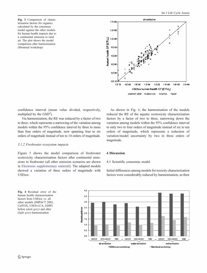
confidence interval (mean value divided, respectively,multiplied by the GSD2).

Via harmonization, the RE was reduced by a factor of twoto three, which represents a narrowing of the variation amongmodels within the 95% confidence interval by three to morethan four orders of magnitude, now spanning four to sixorders of magnitude instead of ten to 14 orders of magnitude.

3.1.2 Freshwater ecosystem impacts

Figure 5 shows the model comparison of freshwaterecotoxicity characterisation factors after continental emis-sions to freshwater (all other emission scenarios are shownin Electronic supplementary material). The adapted modelsshowed a variation of three orders of magnitude withUSEtox.

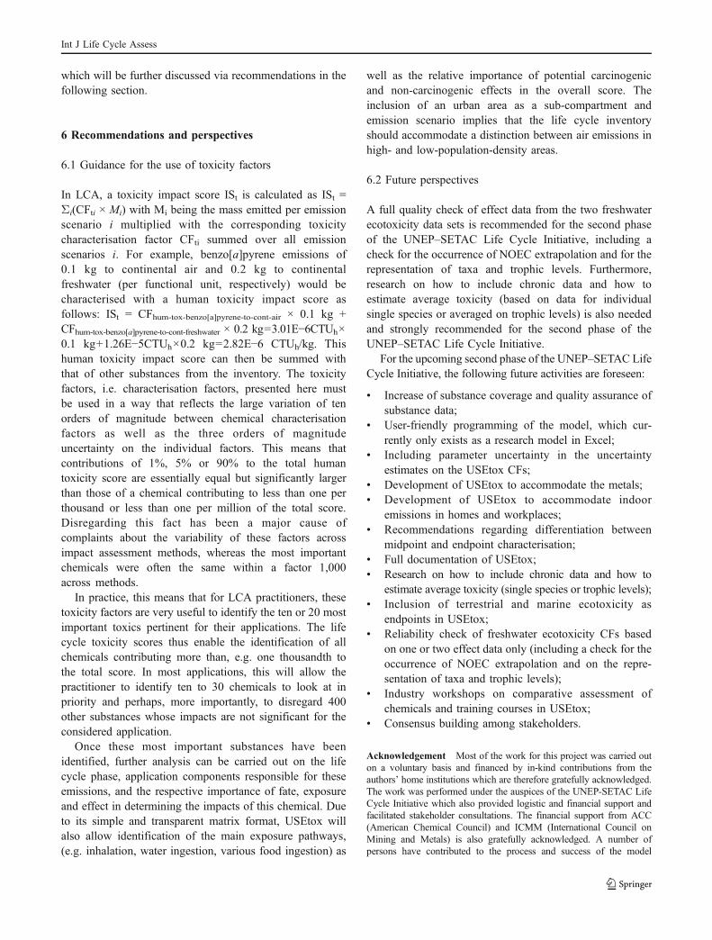
As shown in Fig. 6, the harmonisation of the modelsreduced the RE of the aquatic ecotoxicity characterisationfactors by a factor of two to three, narrowing down thevariation among models within the 95% confidence intervalto only two to four orders of magnitude instead of six to tenorders of magnitude, which represents a reduction ofvariation/model uncertainty by two to three orders ofmagnitude.

4 Discussion

4.1 Scientific consensus model

Initial differences among models for toxicity characterisationfactors were considerably reduced by harmonisation, as their

Fig. 4 Residual error of thehuman health characterisationfactors from USEtox vs. allother models (IMPACT 2002,CalTOX, USES-LCA, EDIP)before (dark grey) and after(light grey) harmonisation

Fig. 3 Comparison of charac-terisation factors for organicscalculated by the consensusmodel against the other modelsfor human health impacts due toa continental emission to ruralair. The plot shows the modelcomparison after harmonisation(Montreal workshop)

Int J Life Cycle Assess

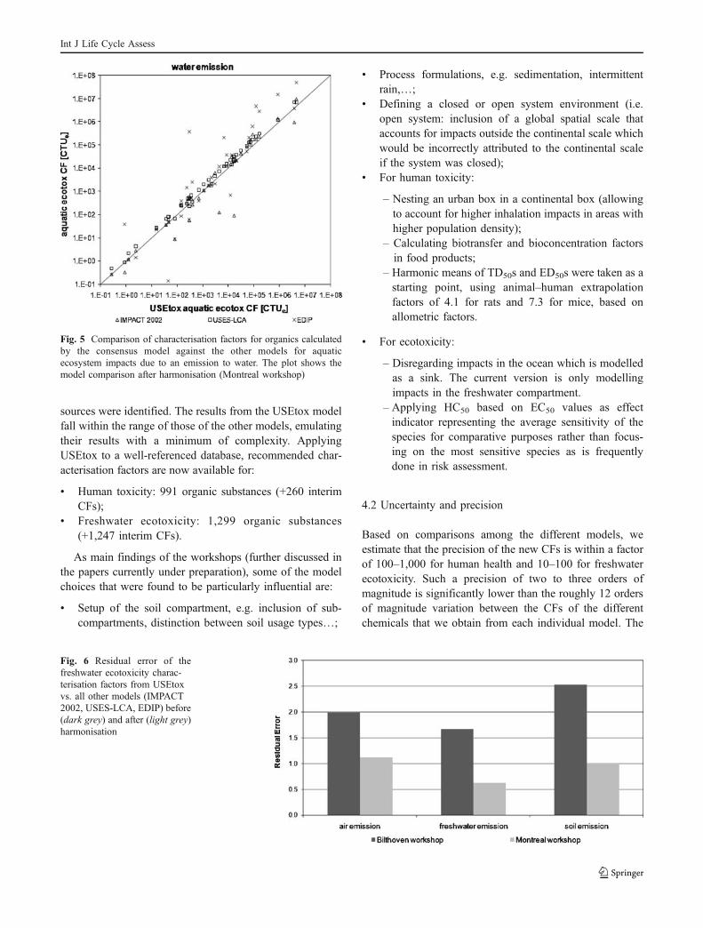
sources were identified. The results from the USEtox modelfall within the range of those of the other models, emulatingtheir results with a minimum of complexity. ApplyingUSEtox to a well-referenced database, recommended char-acterisation factors are now available for:

& Human toxicity: 991 organic substances (+260 interimCFs);

& Freshwater ecotoxicity: 1,299 organic substances(+1,247 interim CFs).

As main findings of the workshops (further discussed inthe papers currently under preparation), some of the modelchoices that were found to be particularly influential are:

& Setup of the soil compartment, e.g. inclusion of sub-compartments, distinction between soil usage types…;

& Process formulations, e.g. sedimentation, intermittentrain,…;

& Defining a closed or open system environment (i.e.open system: inclusion of a global spatial scale thataccounts for impacts outside the continental scale whichwould be incorrectly attributed to the continental scaleif the system was closed);

& For human toxicity:

– Nesting an urban box in a continental box (allowingto account for higher inhalation impacts in areas withhigher population density);

– Calculating biotransfer and bioconcentration factorsin food products;

– Harmonic means of TD50s and ED50s were taken as astarting point, using animal–human extrapolationfactors of 4.1 for rats and 7.3 for mice, based onallometric factors.

& For ecotoxicity:

– Disregarding impacts in the ocean which is modelledas a sink. The current version is only modellingimpacts in the freshwater compartment.

– Applying HC50 based on EC50 values as effectindicator representing the average sensitivity of thespecies for comparative purposes rather than focus-ing on the most sensitive species as is frequentlydone in risk assessment.

4.2 Uncertainty and precision

Based on comparisons among the different models, weestimate that the precision of the new CFs is within a factorof 100–1,000 for human health and 10–100 for freshwaterecotoxicity. Such a precision of two to three orders ofmagnitude is significantly lower than the roughly 12 ordersof magnitude variation between the CFs of the differentchemicals that we obtain from each individual model. The

Fig. 6 Residual error of thefreshwater ecotoxicity charac-terisation factors from USEtoxvs. all other models (IMPACT2002, USES-LCA, EDIP) before(dark grey) and after (light grey)harmonisation

Fig. 5 Comparison of characterisation factors for organics calculatedby the consensus model against the other models for aquaticecosystem impacts due to an emission to water. The plot shows themodel comparison after harmonisation (Montreal workshop)

Int J Life Cycle Assess

uncertainty range in model results is due to variationbetween the models and does not include parameteruncertainties attached to the input data used to calculatethe CFs, as input data were kept the same. As a firstestimate of the underlying model uncertainty (i.e. withoutparameter uncertainty) inherent in the recommended CFs,Table 2 provides their GSD2 under the assumption that theyare log-normally distributed. These estimates are based onthe residual error discussed in Section 3.1.1.

Apart from differences in model structure, importantsources of uncertainty of the USEtox results are, amongothers, the uncertainty and variability related to inputparameters and the lack of accurate mechanistic QSARsto estimate substance properties like carryover rates to meatand milk, limited data on bioconcentration factors for fish,lacking data on chemical degradation rates and largeuncertainties related to both human health and ecotoxiceffect data. The latter comprise issues such as the use ofchronic and acute data, route-to-route extrapolations (i.e.from oral administration in rodent tests to inhalation byhumans) and the application of a linear dose–responsecurve for both the human health and the aquatic ecotoxicityeffect factors calculation. Furthermore, we chose to set thehuman effect factor to zero if no toxicology information isavailable. The assumption of homogenous compartments,even for such complex media as soil or water, represents afurther uncertainty, as in the USEtox model, any chemicalentering these compartments is immediately diluted per-fectly within the volume. The vegetation model used in theexposure model does not include any degradation processbecause data are not available. This will overestimateexposures of humans via agricultural produce and meat/milk, further increasing the uncertainty of biotransferprocesses modelling in USEtox.

Both ‘recommended’ and ‘interim’ characterisationfactors are provided. The main difference between recom-mended and interim characterisation factors is related eitherto the applicability of USEtox to the respective substancesor the availability and quality of the necessary input data.Currently, USEtox is applicable to generic, non-dissociatingand non-amphiphilic organic substances. Notably, it does

not account for speciation and other important specificprocesses for metals, metal compounds, and certain types oforganic chemicals. As the needed improvements in themodelling practice for these groups of compounds are stillunder elaboration, we decided to provide interim factors forthe time being. Furthermore, for a number of chemicals, theminimum data quality could not be met, e.g. for estimationof the aquatic ecotoxicity effect factor in situations wheredata for less than three species were available. This led tothe decision to not actually recommend factors for suchsubstances whilst research is currently ongoing but to atleast provide interim characterisation factors that might beused if needed, but which are not endorsed by the UNEP–SETAC initiative. The uncertainty of these factors is verylarge, but given the overall range of chemical variation,they might be used with caution.

As already mentioned, missing data and knowledgeimpose limitations to the use and interpretation of the modeland its results. We also note that certain human exposureroutes, such as indoor air and dermal exposure are currentlynot included. Limiting factors in terms of data availability arenotably data on human toxicity, ecotoxicity, biotransfer anddegradation. For these important inputs, we had to rely onQSAR methods with all their intrinsic uncertainties. Forother endpoints such as marine or terrestrial ecosystems,almost no experimental data are currently available. Furtherresearch should be undertaken to improve the respective databasis and bridge this data gap.

5 Conclusions

USEtox provides a parsimonious and transparent tool forhuman health and ecosystem CF estimates. It has beencarefully constructed as well as evaluated via comparisonwith other models and falls within the range of their resultswhilst being less complex. It may thus serve as an interfacebetween the more sophisticated state-of-the-art expertmodels (such as those compared in this study and whichfrequently change due to latest scientific developmentsbeing included) and the need of practitioners for transpar-ency, broad stakeholder acceptance and stability of factorsand methods applied in LCA. Based on a referenceddatabase, USEtox has been used to calculate CFs forseveral thousand substances and forms the basis of therecommendations from UNEP–SETAC’s Life Cycle Initia-tive regarding characterisation of toxic impacts in life cycleassessment. USEtox therefore provides the largest sub-stance coverage presently available in term of numbers ofchemicals covered. Furthermore, model uncertainty haspartly been quantified. USEtox thus represents a signifi-cantly improved basis for a wider application of humanhealth and ecotoxicity characterisation factors in LCA

Table 2 Model uncertainty estimates for the recommended character-isation factors

Characterisation factor GSD2

Human health, emission to rural air 77Human health, emission to freshwater 215Human health, emission to agricultural soil 2,189Freshwater ecotoxicity, emission to rural air 176Freshwater ecotoxicity, emission to freshwater 18Freshwater ecotoxicity, emission to agricultural soil 103

Int J Life Cycle Assess

which will be further discussed via recommendations in thefollowing section.

6 Recommendations and perspectives

6.1 Guidance for the use of toxicity factors

In LCA, a toxicity impact score ISt is calculated as ISt =Σi(CFti × Mi) with Mi being the mass emitted per emissionscenario i multiplied with the corresponding toxicitycharacterisation factor CFti summed over all emissionscenarios i. For example, benzo[a]pyrene emissions of0.1 kg to continental air and 0.2 kg to continentalfreshwater (per functional unit, respectively) would becharacterised with a human toxicity impact score asfollows: ISt = CFhum-tox-benzo[a]pyrene-to-cont-air × 0.1 kg +CFhum-tox-benzo[a]pyrene-to-cont-freshwater × 0.2 kg=3.01E−6CTUh×0.1 kg+1.26E−5CTUh×0.2 kg=2.82E−6 CTUh/kg. Thishuman toxicity impact score can then be summed withthat of other substances from the inventory. The toxicityfactors, i.e. characterisation factors, presented here mustbe used in a way that reflects the large variation of tenorders of magnitude between chemical characterisationfactors as well as the three orders of magnitudeuncertainty on the individual factors. This means thatcontributions of 1%, 5% or 90% to the total humantoxicity score are essentially equal but significantly largerthan those of a chemical contributing to less than one perthousand or less than one per million of the total score.Disregarding this fact has been a major cause ofcomplaints about the variability of these factors acrossimpact assessment methods, whereas the most importantchemicals were often the same within a factor 1,000across methods.

In practice, this means that for LCA practitioners, thesetoxicity factors are very useful to identify the ten or 20 mostimportant toxics pertinent for their applications. The lifecycle toxicity scores thus enable the identification of allchemicals contributing more than, e.g. one thousandth tothe total score. In most applications, this will allow thepractitioner to identify ten to 30 chemicals to look at inpriority and perhaps, more importantly, to disregard 400other substances whose impacts are not significant for theconsidered application.

Once these most important substances have beenidentified, further analysis can be carried out on the lifecycle phase, application components responsible for theseemissions, and the respective importance of fate, exposureand effect in determining the impacts of this chemical. Dueto its simple and transparent matrix format, USEtox willalso allow identification of the main exposure pathways,(e.g. inhalation, water ingestion, various food ingestion) as

well as the relative importance of potential carcinogenicand non-carcinogenic effects in the overall score. Theinclusion of an urban area as a sub-compartment andemission scenario implies that the life cycle inventoryshould accommodate a distinction between air emissions inhigh- and low-population-density areas.

6.2 Future perspectives

A full quality check of effect data from the two freshwaterecotoxicity data sets is recommended for the second phaseof the UNEP–SETAC Life Cycle Initiative, including acheck for the occurrence of NOEC extrapolation and for therepresentation of taxa and trophic levels. Furthermore,research on how to include chronic data and how toestimate average toxicity (based on data for individualsingle species or averaged on trophic levels) is also neededand strongly recommended for the second phase of theUNEP–SETAC Life Cycle Initiative.

For the upcoming second phase of the UNEP–SETAC LifeCycle Initiative, the following future activities are foreseen:

& Increase of substance coverage and quality assurance ofsubstance data;

& User-friendly programming of the model, which cur-rently only exists as a research model in Excel;

& Including parameter uncertainty in the uncertaintyestimates on the USEtox CFs;

& Development of USEtox to accommodate the metals;& Development of USEtox to accommodate indoor

emissions in homes and workplaces;& Recommendations regarding differentiation between

midpoint and endpoint characterisation;& Full documentation of USEtox;& Research on how to include chronic data and how to

estimate average toxicity (single species or trophic levels);& Inclusion of terrestrial and marine ecotoxicity as

endpoints in USEtox;& Reliability check of freshwater ecotoxicity CFs based

on one or two effect data only (including a check for theoccurrence of NOEC extrapolation and on the repre-sentation of taxa and trophic levels);

& Industry workshops on comparative assessment ofchemicals and training courses in USEtox;

& Consensus building among stakeholders.

Acknowledgement Most of the work for this project was carried outon a voluntary basis and financed by in-kind contributions from theauthors’ home institutions which are therefore gratefully acknowledged.The work was performed under the auspices of the UNEP-SETAC LifeCycle Initiative which also provided logistic and financial support andfacilitated stakeholder consultations. The financial support from ACC(American Chemical Council) and ICMM (International Council onMining and Metals) is also gratefully acknowledged. A number ofpersons have contributed to the process and success of the model

Int J Life Cycle Assess

comparison and scientific consensusmodel development. The authors aregrateful for the participation of Miriam Diamond, Louise Deschênes, BillAdams, Andrea Russel, Jeroen Guinée, Pierre-Yves Robidoux, StefanieHellweg, Evangelia Demou, Stig Irving Olsen, Cécile Bulle, Sau SoonChen, Manuel Olivera, Julian Marshall, Bert-Droste Franke, PeterFantke, Oleg Travnikov, Dick de Zwart, Peter Chapman, Kees vanGestel and Thomas H. Slone.

References

Aronson D, Boethling R, Howard P, Stiteler, W (2006) Estimatingbiodegradation half-lives for use in chemical screening. Chemo-sphere 63(11):1953–1960

Bachmann TM (2006) Hazardous substances and human health:exposure, impact and external cost assessment at the Europeanscale. Trace metals and other contaminants in the environment, 8.Elsevier, Amsterdam, p 570

Bennett DH, Scheringer M, McKone TE, Hungerbühler K (2001)Predicting long-range transport: a systematic evaluation of twomultimedia transport models. Environ Sci Technol 35(6):1181

Cowan CE, Mackay D, Feijtel TCJ, van de Meent D, Di Guardo A,Davies J, Mackay N (eds) (1994) The multi-media fate model: avital tool for predicting the fate of chemicals. SETAC. SETACPress, Denver, CO

Dreyer LC, Niemann AL, Hauschild MZ (2003) Comparison of threedifferent LCIA methods: EDIP97, CML2001 and Eco-Indicator99: does it matter which one you choose? Int J Life Cycle Assess8(4):191–200

EC (1999) Externalities of fuel cycles—ExternE Project. Vol. 7—methodology, 2nd edn. European Commission DG XII, ScienceResearch and Development, JOULE, Brussels, Luxembourg

EC (2003) Technical guidance document on risk assessment inSupport of Commission Directive 93/67/EEC on Risk Assessmentfor new notified substances. Commission Regulation (EC) no. 1488/94 on risk assessment for existing substances. Directive 98/8/EC ofthe European Parliament and of the Council concerning the placingof biocidal products on the market—part I, Institute for Health andConsumer Protection, European Chemicals Bureau, European JointResearch Centre (JRC) Ispra, Italy

EC (2005) ExternE—externalities of energy: Methodology 2005update. Office for Official Publication of the European Commu-nities, Luxembourg

ECOTOX (2001) ECOTOXicology Database system. http://www.epa.gov/ecotox

Fenner K, Scheringer M, Stroebe M, Macleod M, McKone T,Matthies M, Klasmeier J, Beyer A, Bonnell M, Le Gall AC,Mackay D, Van De Meent D, Pennington D, Scharenberg B,Suzuki N, Wania F (2005) Comparing estimates of persistenceand long-range transport potential among multimedia models.Environ Sci Technol 39(7):1932

Goedkoop M, Müller-Wenk R, Hofstetter P, Spriensma R (1998) TheEco-Indicator 99 explained. Int J Life Cycle Assess 3(6):352–360

Gold LS, Slone TH, Bernstein L (1989) Summary of carcinogenicpotency and positivity for 492 rodent carcinogens in thecarcinogenic potency database. Environ Health Perspect79:259–272

Gold LS, Manley NB, Slone TH, Rohrbach L, Backman-Garfinkel G(2005) Supplement to the carcinogenic potency database (CPDB)Results of animal bioassays published in the general literaturethrough 1997 and by the National Toxicology Program in 1997–1998. Toxicol Sci 85(2):747–808

Gold LS et al (2008) The carcinogenic potency database (CPDB).http://potency.berkeley.edu/chemicalsummary.html

Hauschild M, Wenzel H (1998) Environmental assessment ofproducts, vol 2: scientific background. Kluwer, Hingham, MA,USA, p 565

Hauschild MZ, Huijbregts MAJ, Jolliet O, MacLeod M, Margni M,van de Meent D, Rosenbaum RK, McKone TE (2008) Building amodel based on scientific consensus for life cycle impactassessment of chemicals: the search for harmony and parsimony.Environ Sci Technol 42(19):7032–7037

Heijungs R, Guinée JB, Huppes G, Lankreijer RM, Udo de Haes HA,Wegner Sleeswijk A, Ansems AMM, Eggels PG, van Duin R,Goede AP (1992) Environmental life cycle assessment of products.Centre of Environmental Sciences, Leiden, The Netherlands

Hertwich E, Matales SF, Pease WS, McKone TE (2001) Humantoxicity potentials for life-cycle assessment and toxics releaseinventory risk screening. Environ Toxicol Chem 20(4):928–939

Howard PH, Meylan WM (eds) (1997) Handbook of physicalproperties of organic chemicals. Lewis Publishers (CRC Presscop), Michigan, 1585 pp

Howard PH, Boethling RS, Jarvis WF, Meylan WM, Michalenko EM(1991) Handbook of environmental degradation rates. LewisPublishers, Michigan

Huijbregts MAJ, Thissen U, Guinée JB, Jager T, Kalf D, van deMeent D, Ragas AMJ, Wegener Sleeswijk A, Reijnders L (2000)Priority assessment of toxic substances in life cycle assessment.Part I: calculation of toxicity potentials for 181 substances with thenested multi-media fate, exposure and effects model USES-LCA.Chemosphere 41(4):541–573

Huijbregts MAJ, Geelen LMJ, Van De Meent D, Hertwich EG,McKone TE (2005a) A comparison between the multimedia fateand exposure models CalTOX and uniform system for evaluationof substances adapted for life-cycle assessment based on thepopulation intake fraction of toxic pollutants. Environ ToxicolChem 24(2):486–493

Huijbregts MAJ, Rombouts LJA, Ragas AMJ, Van de Meent D(2005b) Human-toxicological effect and damage factors ofcarcinogenic and noncarcinogenic chemicals for life cycle impactassessment. Integr Environ Assess Manage 1(3):181–192

Huijbregts MAJ, Struijs J, Goedkoop M, Heijungs R, Hendriks AJ,Van de Meent D (2005c) Human population intake fractions andenvironmental fate factors of toxic pollutants in life cycle impactassessment. Chemosphere 61(10):1495–1504

IUCLID (2000) IUCLID CD-ROM Year 2000 edition. Public data onhigh volume chemicals

Jolliet O, Hauschild M (2005) The influence of the intermittentcharacter of rain on fate and long range transport of air organicpollutants. Environ Sci Technol 39(12):4513–4522

Jolliet O, Brent A, Goedkoop M, Itsubo N, Mueller-Wenk R, Peña C,Schenk R, Stewart M, Weidema B (2003a) The LCIA Frame-work. SETAC–UNEP Life Cycle Initiative, Lausanne

Jolliet O, Margni M, Charles R, Humbert S, Payet J, Rebitzer G,Rosenbaum RK (2003b) IMPACT 2002+: a new life cycle impactassessment methodology. Int J Life Cycle Assess 8(6):324–330

Jolliet O, Rosenbaum RK, Chapmann P, McKone T, Margni M,Scheringer M, van Straalen N, Wania F (2006) Establishing aframework for life cycle toxicity assessment: findings of theLausanne review workshop. Int J Life Cycle Assess 11(3):209–212

Kawamoto K, MacLeod M, Mackay D (2001) Evaluation andcomparison of multimedia mass balance models of chemicalfate: Application of EUSES and ChemCAN to 68 chemicals inJapan. Chemosphere 44(4):599–612

Larsen HF, Hauschild MZ (2007) GM-troph: a low data demandecotoxicity effect indicator for use in LCIA. Int J Life CycleAssess 12(2):79–91

Ligthart T et al (2004) Declaration of Apeldoorn on LCIA of Non-Ferrous Metals. http://lcinitiative.unep.fr/includes/file.asp?site=l-cinit&file=38D1F49D-6D64-45AE-9F64-578BA414E499

Int J Life Cycle Assess

Mackay D, Seth R (1999) The role of mass balance modelling inimpact assessment and pollution prevention. In: Sikdar SK,Diweakar U (eds) Tools and methods for pollution prevention.Kluwer, The Netherlands, pp 157–179

Mackay D, Shiu WY, Lee SC, Ma KC (2006) Handbook of physical–chemical properties and environmental fate for organic chem-icals. Science, Technology, Engineering, I–IV. CRC, Boca Raton

MacLeod M, Woodfine DG, Mackay D, McKone TE, Bennett DH,Maddalena R (2001) BETR North America: a regionallysegmented multimedia contaminant fate model for North America.Environ Sci Pollut Res 8(3):156–163

Maddalena RL,McKone TE, LaytonDW,Hsieh DPH (1995) Comparisonof multi-media transport and transformation models: regionalfugacity model vs. CalTOX. Chemosphere 30(5):869–899

Margni M (2003) Source to intake modeling in life cycle impactassessment. PhD thesis, Ecole Polytechnique Fédérale deLausanne (EPFL), Lausanne, Switzerland, 138 pp

Margni M, Pennington DW, Birkved M, Larsen HF, Hauschild M(2002) Test set of organic chemicals for LCIA characterisationmethod comparison. OMNITOX project report

Margni M, Pennington DW, Bennett DH, Jolliet O (2004) Cyclicexchanges and level of coupling between environmental media:intermedia feedback in multimedia fate models. Environ SciTechnol 38(20):5450–5457

McKone TE (1993) The precision of QSAR methods for estimatingintermedia transfer factors in exposure assessments. SAR QSAREnviron Res 1(1):41–51

McKone TE (2001) Ecological toxicity potentials (ETPs) forsubstances released to air and surface waters. EnvironmentalHealth Sciences Division, School of Public Health, University ofCalifornia, Berkeley, CA 94720

McKone T, Bennett D, Maddalena R (2001) CalTOX 4.0 Technicalsupport document, vol 1. LBNL-47254, Lawrence BerkeleyNational Laboratory, Berkeley, CA

McKone TE, Kyle AD, Jolliet O, Olsen SI, Hauschild M (2006)Dose–response modeling for life cycle impact assessment—findings of the Portland Review Workshop. Int J Life CycleAssess 11(2):137–140

Meylan WM, Howard PH, Boethling RS, Aronson D, Printup H,Gouchie S (1999) Improvedmethod for estimating bioconcentration/bioaccumulation factor from octanol/water partition coefficient.Environ Toxicol Chem 18(4):664–672

NCMS (2008) SOLV-DB. http://solvdb.ncms.org/index.htmlPant R, Van Hoof G, Schowanek D, Feijtel TCJ, De Koning A,

Hauschild M, Olsen SI, Pennington DW, Rosenbaum RK (2004)Comparison between three different LCIA methods for aquaticecotoxicity and a product environmental risk assessment: insightsfrom a detergent case study within OMNIITOX. Int J Life CycleAssess 9(5):295–306

Payet J (2004) Assessing toxic impacts on aquatic ecosystems in lifecycle assessment (LCA). PhD thesis, Ecole PolytechniqueFédérale de Lausanne (EPFL), Lausanne, Switzerland, 190 pp

Pennington DW, Margni M, Ammann C, Jolliet O (2005) Multimediafate and human intake modeling: spatial versus nonspatialinsights for chemical emissions in Western Europe. Environ SciTechnol 39(4):1119–1128

Rosenbaum RK (2006) Multimedia and food chain modelling oftoxics for comparative risk and life cycle impact assessment. PhDthesis, Ecole Polytechnique Fédérale de Lausanne (EPFL),Lausanne, Switzerland, 192 pp

Rosenbaum RK, Margni M, Jolliet O (2007) A flexible matrix algebraframework for the multimedia multipathway modeling ofemission to impacts. Environ Int 33(5):624–634

Scheringer M, Wegmann F, Hungerbühler K (2004) Investigating themechanics of multimedia box models: how to explain differencesbetween models in terms of mass fluxes? Environ Toxicol Chem23(10):2433–2440

Sinkkonen S, Paasivirta J (2000) Degradation half-life times ofPCDDs, PCDFs and PCBs for environmental fate modeling.Chemosphere 40(9):943–949

SRC (2008) Environmental Fate Data Base (EFDB). http://www.syrres.com/esc/efdb.htm

Stroebe M, Scheringer M, Hungerbühler K, Held H (2004) Inter-comparison of multimedia modeling approaches: modes oftransport, measures of long range transport potential and thespatial remote state. Sci Total Environ 321(1–3):1–20

Travis C, Arms A (1988) Bioconcentration of organics in beef, milk,and vegetation. Environ Sci Technol 22(3):271–274

USEPA (2007) Estimation Programs Interface EPI Suite. http://www.epa.gov/opptintr/exposure/pubs/episuite.htm

Van Zelm R, Huijbregts MAJ, Harbers JV, Wintersen A, Struijs J,Posthuma L, Van de Meent D (2007) Uncertainty in msPAF-basedecotoxicological effect factors for freshwater ecosystems in life cycleimpact assessment. Integr Environ Assess Manage 3(2):203–210

Vermeire T, Pieters M, Rennen M, Bos P (2001) Probabalisticassessment factors for human health risk assessment—a practicalguide. National Institute for Health and the Environment,Bilthoven, The Netherlands

Wania F, Dugani CB (2003) Assessing the long-range transportpotential of polybrominated diphenyl ethers: a comparison of fourmultimedia models. Environ Toxicol Chem 22(6):1252–1261

Wania F, MacKay D (2000) A comparison of overall persistencevalues and atmospheric travel distances calculated by variousmulti-media fate models. WECC Wania Environmental ChemistsCorp., under Chlorine Chemistry Council Contracts No. 9461and 9462, Toronto, Ontario, Canada

Wegmann F, Cavin L, MacLeod M, Scheringer M, Hungerbühler K(2008) A software tool for screening chemicals of environmentalconcern for persistence and long-range transport potential.Environ Model Softw 24(2):228–237 http://dx.doi.org/10.1016/j.envsoft.2008.06.014

Wenzel H, Hauschild M, Alting L (1998) Environmental assessmentof products, vol 1: methodology, tools and case studies in productdevelopment. Kluwer, Hingham, MA, USA, p 560

Int J Life Cycle Assess