USER'S GUIDE FOR TOMLAB /KNITRO v5 - MATLAB OPTIMIZATION and .NET

USER’S GUIDE FOR TOMLAB /KNITRO v61

Kenneth Holmstrom2, Anders O. Goran3 and Marcus M. Edvall4

August 11, 2009

1More information available at the TOMLAB home page: http://tomopt.com. E-mail: [email protected] in Optimization, Malardalen University, Department of Mathematics and Physics, P.O. Box 883, SE-721 23 Vasteras,

Sweden, [email protected] Optimization AB, Vasteras Technology Park, Trefasgatan 4, SE-721 30 Vasteras, Sweden, [email protected] Optimization Inc., 1260 SE Bishop Blvd Ste E, Pullman, WA, USA, [email protected] c©2004-2008 Tomlab Optimization Inc. and c©2004-2008 Ziena Optimization, Inc.

1

http://tomopt.com

mailto:[email protected]




Contents

Contents 2

1 Introduction 3

1.1 Overview . . . . . . . . . . . . . . . . . . . . . . . . . . . . . . . . . . . . . . . . . . . . . . . . . . 3

1.2 Contents of this Manual . . . . . . . . . . . . . . . . . . . . . . . . . . . . . . . . . . . . . . . . . . 3

1.3 More information . . . . . . . . . . . . . . . . . . . . . . . . . . . . . . . . . . . . . . . . . . . . . . 4

1.4 Prerequisites . . . . . . . . . . . . . . . . . . . . . . . . . . . . . . . . . . . . . . . . . . . . . . . . 4

2 Using the Matlab Interface 5

3 Setting KNITRO options 5

3.1 Setting options using the KNITRO.options structure . . . . . . . . . . . . . . . . . . . . . . . . . . 5

4 TOMLAB /KNITRO Solver Reference 6

4.1 knitroTL . . . . . . . . . . . . . . . . . . . . . . . . . . . . . . . . . . . . . . . . . . . . . . . . . . 6

5 Termination Test and Optimality 26

6 TOMLAB /KNITRO Output 28

7 Algorithm Options 30

7.1 Automatic . . . . . . . . . . . . . . . . . . . . . . . . . . . . . . . . . . . . . . . . . . . . . . . . . . 30

7.2 Interior/Direct . . . . . . . . . . . . . . . . . . . . . . . . . . . . . . . . . . . . . . . . . . . . . . . 30

7.3 Interior/CG . . . . . . . . . . . . . . . . . . . . . . . . . . . . . . . . . . . . . . . . . . . . . . . . . 30

7.4 Active . . . . . . . . . . . . . . . . . . . . . . . . . . . . . . . . . . . . . . . . . . . . . . . . . . . . 30

8 Other special features 31

8.1 First derivative and gradient check options . . . . . . . . . . . . . . . . . . . . . . . . . . . . . . . 31

8.2 Second derivative options . . . . . . . . . . . . . . . . . . . . . . . . . . . . . . . . . . . . . . . . . 31

8.3 Feasible version . . . . . . . . . . . . . . . . . . . . . . . . . . . . . . . . . . . . . . . . . . . . . . . 32

8.4 Honor Bounds . . . . . . . . . . . . . . . . . . . . . . . . . . . . . . . . . . . . . . . . . . . . . . . . 33

8.5 Crossover . . . . . . . . . . . . . . . . . . . . . . . . . . . . . . . . . . . . . . . . . . . . . . . . . . 33

8.6 Multi-start . . . . . . . . . . . . . . . . . . . . . . . . . . . . . . . . . . . . . . . . . . . . . . . . . 34

8.7 Solving Systems of Nonlinear Equations . . . . . . . . . . . . . . . . . . . . . . . . . . . . . . . . . 34

8.8 Solving Least Squares Problems . . . . . . . . . . . . . . . . . . . . . . . . . . . . . . . . . . . . . . 34

8.9 Mathematical programs with equilibrium constraints (MPECs) . . . . . . . . . . . . . . . . . . . . 35

8.10 Global optimization . . . . . . . . . . . . . . . . . . . . . . . . . . . . . . . . . . . . . . . . . . . . 36

2

1 Introduction

1.1 Overview

Welcome to the TOMLAB /KNITRO User’s Guide. TOMLAB /KNITRO includes the KNITRO (MI)NLP solverfrom Ziena Optimization and an interface to The MathWorks’ MATLAB.

Knitro implements both state-of-the-art interior-point and active-set methods for solving nonlinear optimiza-tion problems. In the interior method (also known as a barrier method), the nonlinear programming prob-lem is replaced by a series of barrier sub-problems controlled by a barrier parameter µ (initial value set usingProb.KNITRO.options.BAR INITMU). The algorithm uses trust regions and a merit function to promote con-vergence. The algorithm performs one or more minimization steps on each barrier problem, then decreases thebarrier parameter, and repeats the process until the original problem has been solved to the desired accuracy.

Knitro provides two procedures for computing the steps within the interior point approach. In the version knownas Interior/CG each step is computed using a projected conjugate gradient iteration. This approach differs frommost interior methods proposed in the literature in that it does not compute each step by solving a linear systeminvolving the KKT (or primal-dual) matrix. Instead, it factors a projection matrix, and uses the conjugate gradientmethod, to approximately minimize a quadratic model of the barrier problem.

The second procedure for computing the steps, which we call Interior/Direct, always attempts to compute anew iterate by solving the primal-dual KKT matrix using direct linear algebra. In the case when this step cannotbe guaranteed to be of good quality, or if negative curvature is detected, then the new iterate is computed by theInterior/CG procedure.

Knitro also implements an active-set sequential linear-quadratic programming (SLQP) algorithm which we callActive. This method is similar in nature to a sequential quadratic programming method but uses linear program-ming sub-problems to estimate the active-set at each iteration. This active-set code may be preferable when agood initial point can be provided, for example, when solving a sequence of related problems.

Knitro has support for mixed-integer programming, either by a standard branch and bound method or a hybridQuesada-Grossman method.

We encourage the user to try all algorithmic options to determine which one is more suitable for the applicationat hand. For guidance on choosing the best algorithm see Section 7.

1.2 Contents of this Manual

• Section 1 provides a basic overview of the KNITRO solver.

• Section 2 provides an overview of the Matlab interface to KNITRO.

• Section 3 describes how to set KNITRO solver options from Matlab.

• Section 4 gives detailed information about the interface routine knitroTL.

• Section 5 shows how the solver terminates.

• Section 6 details the solver output.

• Section 7 provides detailed information about the algorithmic options available.

• Section 8 discusses some of the options and features in TOMLAB /KNITRO.

3

1.3 More information

Please visit the following links for more information:

• http://tomopt.com/tomlab/products/knitro/

1.4 Prerequisites

In this manual we assume that the user is familiar with nonlinear programming, setting up problems in TOMLAB(in particular constrained nonlinear (con) problems) and the Matlab language in general.

4

http://tomopt.com/tomlab/products/knitro/

2 Using the Matlab Interface

The KNITRO solver is accessed via the tomRun driver routine, which calls the knitroTL interface routine. Thesolver itself is located in the MEX file Tknitro.

Table 1: The interface routines.

Function Description Section PageknitroTL The interface routine called by the TOMLAB driver routine tomRun.

This routine then calls the MEX file Tknitro4.1 6

3 Setting KNITRO options

All KNITRO control parameters are possible to set from Matlab. To get intermediate results printed to theMatlab command window, use the Prob.PriLevOpt parameter.

3.1 Setting options using the KNITRO.options structure

The parameters can be set as subfields in the Prob.KNITRO.options structure. The following example shows howto set a limit on the maximum number of iterations, and selecting the feasible version of KNITRO:

Prob = conAssign(...) % Setup problem, see help conAssign for more information

Prob.KNITRO.options.MAXIT = 200; % Setting maximum number of iterations

Prob.KNITRO.options.BAR_FEASIBLE = 1; % Select feasible KNITRO

The maximum number of iterations can also be done through the TOMLAB parameter MaxIter:

Prob.optParam.MaxIter = 200;

In the cases where a solver specific parameter has a corresponding TOMLAB general parameter, the latter is usedonly if the user has not given the solver specific parameter.

A complete description of the available KNITRO parameters can be found in Section 4.1.

5

4 TOMLAB /KNITRO Solver Reference

A detailed description of the TOMLAB /KNITRO solver interface is given below. Also see the M-file help forknitroTL.m.

4.1 knitroTL

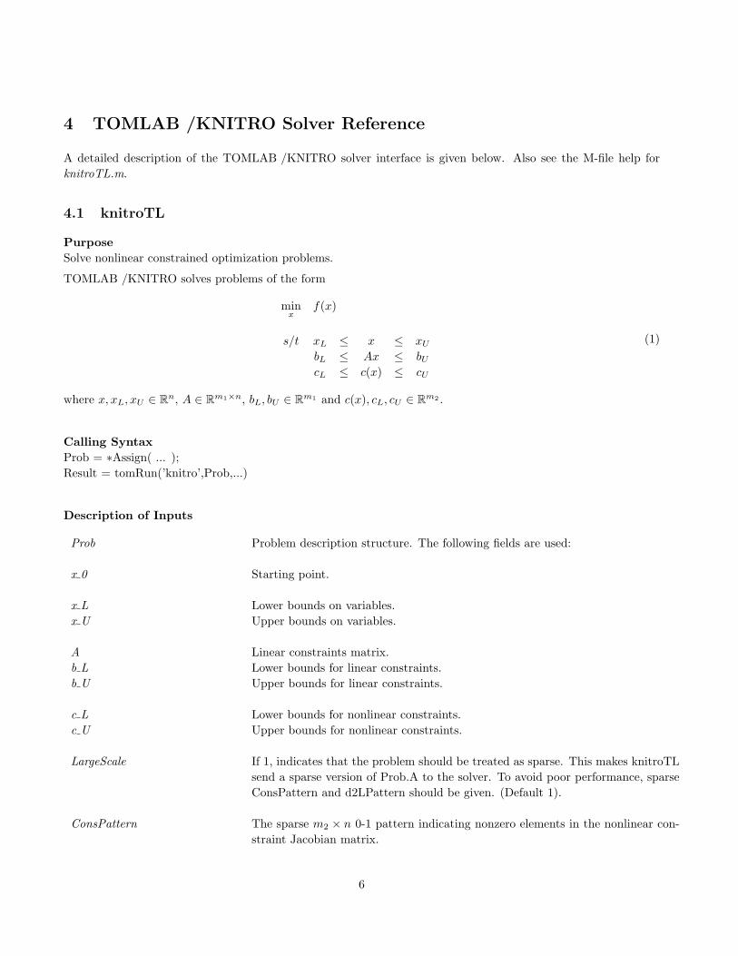
PurposeSolve nonlinear constrained optimization problems.

TOMLAB /KNITRO solves problems of the form

minx

f(x)

s/t xL ≤ x ≤ xU

bL ≤ Ax ≤ bUcL ≤ c(x) ≤ cU

(1)

where x, xL, xU ∈ Rn, A ∈ Rm1×n, bL, bU ∈ Rm1 and c(x), cL, cU ∈ Rm2 .

Calling SyntaxProb = ∗Assign( ... );Result = tomRun(’knitro’,Prob,...)

Description of Inputs

Prob Problem description structure. The following fields are used:

x 0 Starting point.

x L Lower bounds on variables.x U Upper bounds on variables.

A Linear constraints matrix.b L Lower bounds for linear constraints.b U Upper bounds for linear constraints.

c L Lower bounds for nonlinear constraints.c U Upper bounds for nonlinear constraints.

LargeScale If 1, indicates that the problem should be treated as sparse. This makes knitroTLsend a sparse version of Prob.A to the solver. To avoid poor performance, sparseConsPattern and d2LPattern should be given. (Default 1).

ConsPattern The sparse m2 × n 0-1 pattern indicating nonzero elements in the nonlinear con-straint Jacobian matrix.

6

Prob Problem description structure. The following fields are used:, continued

d2LPattern The sparse n × n 0-1 pattern indicating nonzero elements in the Hessian of theLagrangian function f(x) + λc(x).

f Low A lower bound on the objective function value. KNITRO will stop if it finds an xfor which f(x) <= fLow.

PriLevOpt Print level in solver. TOMLAB /KNITRO supports solver progress informationbeing printed to the MATLAB command window as well as to a file.

For output only to the command window: set PriLevOpt to a positive value (1-6)and set:

Prob.KNITRO.PrintFile = ”;

If PrintFile is set to a valid filename, the same information will be written to thefile (if PriLevOpt is nonzero).or printing only to the PrintFile, set a name (or knitro.txt will be used) and anegative PriLevOpt value. For example:

Prob.KNITRO.PrintFile = ’myprob.txt’;Prob.PriLevOpt = -2;

To run TOMLAB /KNITRO silently, set PriLevOpt=0;

0: Printing of all output is suppressed (default).

1: Only summary information is printed.

2: Information every 10 major iterations is printed where a major iteration is definedby a new solution estimate.

3: Information at each major iteration is printed.

4: Information is printed at each major and minor iteration where a minor iterationis defined by a trial iterate.

5: In addition, the values of the solution vector x are printed.

6: In addition, the values of the constraints c and Lagrange multipliers lambda areprinted.

KNITRO Structure with special fields for KNITRO parameters. Fields used are:

PrintFile Name of file to print solver progress and status information to. Please seePriLevOpt parameter described above.

7


options Structure with KNITRO options. Any element not given is replaced by a defaultvalue, in some cases fetched from standard Tomlab parameters.

ALG Indicates which optimization algorithm to use to solve the problem. Default 0.

0: automatic algorithm selection.

1: Interior/Direct algorithm.

2: Interior/CG algorithm.

3: Active algorithm, SLQP.

BAR FEASIBLE Specifies whether special emphasis is placed on getting and staying feasible in theinterior-point algorithms.

0: No special emphasis on feasibility (default).

1: Iterates must satisfy inequality constraints once they become sufficiently feasi-ble.

2: Special emphasis is placed on getting feasible before trying to optimize.

3: Implement both options 1 and 2 above.

If ”bar feasible=1” or ”bar feasible=3”, this will activate the feasible version ofKnitro. The feasible version of Knitro will force iterates to strictly satisfy in-equalities, but does not require satisfaction of equality constraints at intermediateiterates (see section 8.3). This option and the ”honorbnds” option may be usefulin applications where functions are undefined outside the region defined by in-equalities. The initial point must satisfy inequalities to a sufficient degree; if not,Knitro may generate infeasible iterates and does not switch to the feasible versionuntil a sufficiently feasible point is found. Sufficient satisfaction occurs at a pointx if it is true for all inequalities that,

cl + tol ≤ c(x) ≤ cu− tol (2)

(for cl 6= cu). The constant tol is determined by the option bar feasmodetol.If ”bar feasible=2” or ”bar feasible=3”, Knitro will place special emphasis on firsttrying to get feasible before trying to optimize.

BAR FEASMODETOL Specifies the tolerance in equation 2 that determines whether Knitro will forcesubsequent iterates to remain feasible. The tolerance applies to all inequality con-straints in the problem. This option only has an effect if option ”bar feasible=1”or ”bar feasible=3”. Default 1e− 4.

8


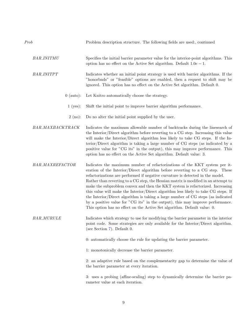
BAR INITMU Specifies the initial barrier parameter value for the interior-point algorithms. Thisoption has no effect on the Active Set algorithm. Default 1.0e− 1.

BAR INITPT Indicates whether an initial point strategy is used with barrier algorithms. If the”honorbnds” or ”feasible” options are enabled, then a request to shift may beignored. This option has no effect on the Active Set algorithm. Default 0.

0 (auto): Let Knitro automatically choose the strategy.

1 (yes): Shift the initial point to improve barrier algorithm performance.

2 (no): Do no alter the initial point supplied by the user.

BAR MAXBACKTRACK Indicates the maximum allowable number of backtracks during the linesearch ofthe Interior/Direct algorithm before reverting to a CG step. Increasing this valuewill make the Interior/Direct algorithm less likely to take CG steps. If the In-terior/Direct algorithm is taking a large number of CG steps (as indicated by apositive value for ”CG its” in the output), this may improve performance. Thisoption has no effect on the Active Set algorithm. Default value: 3.

BAR MAXREFACTOR Indicates the maximum number of refactorizations of the KKT system per it-eration of the Interior/Direct algorithm before reverting to a CG step. Theserefactorizations are performed if negative curvature is detected in the model.Rather than reverting to a CG step, the Hessian matrix is modified in an attempt tomake the subproblem convex and then the KKT system is refactorized. Increasingthis value will make the Interior/Direct algorithm less likely to take CG steps. Ifthe Interior/Direct algorithm is taking a large number of CG steps (as indicatedby a positive value for ”CG its” in the output), this may improve performance.This option has no effect on the Active Set algorithm. Default value: 0.

BAR MURULE Indicates which strategy to use for modifying the barrier parameter in the interiorpoint code. Some strategies are only available for the Interior/Direct algorithm.(see Section 7). Default 0.

0: automatically choose the rule for updating the barrier parameter.

1: monotonically decrease the barrier parameter.

2: an adaptive rule based on the complementarity gap to determine the value ofthe barrier parameter at every iteration.

3: uses a probing (affine-scaling) step to dynamically determine the barrier pa-rameter value at each iteration.

9


4: uses a Mehrotra predictor-corrector type rule to determine the barrier parameterwith safeguards on the corrector step.

5: uses a Mehrotra predictor-corrector type rule to determine the barrier parameterwithout safeguards on the corrector step.

6: minimizes a quality function at each iteration to determine the barrier param-eter.

NOTE: Only strategies 0-2 are available for the Interior/CG algorithm. All strate-gies are available for the Interior/Direct algorithm. Strategies 4 and 5 are typicallyrecommended for linear programs or convex quadratic programs. Many problemsbenefit from a non-default setting of this option and it is recommended to ex-periment with all settings. In particular we recommend trying strategy 6 whenusing the Interior/Direct algorithm. This parameter is not applicable to the Activealgorithm.

BAR PENCONS Indicates whether a penalty approach is applied to the constraints. Using a penaltyapproach may be helpful when the problem has degenerate or difficult constraints.It may also help to more quickly identify infeasible problems, or achieve feasibilityin problems with difficult constraints. This option has no effect on the Active Setalgorithm. Default 0.


1 (none): No constraints are penalized.

2 (all): A penalty approach is applied to all general constraints.

BAR PENRULE Indicates which penalty parameter strategy to use for determining whether or notto accept a trial iterate. This option has no effect on the Active Set algorithm.Default 0.


1 (single): Use a single penalty parameter in the merit function to weight feasibilityversus optimality.

2 (flex): Use a more tolerant and flexible step acceptance procedure based on arange of penalty parameter values.

BLASOPTION Specifies the BLAS/LAPACK function library to use for basic vector and matrixcomputations. Default 0.

0: Use KNITRO builtin functions.

10


1: Use Intel MKL functions.

NOTE: BLAS and LAPACK functions from the Intel Math Kernel Library (MKL)8.1 are provided with the Knitro distribution.

BLAS (Basic Linear Algebra Subroutines) and LAPACK (Linear Algebra PACK-age) functions are used throughout Knitro for fundamental vector and matrixcalculations. The CPU time spent in these operations can be measured by settingoption ”debug=1” and examining the output file kdbg summ*.txt. Some optimiza-tion problems are observed to spend less than 1% of CPU time in BLAS/LAPACKoperations, while others spend more than 50%. Be aware that the different func-tion implementations can return slightly different answers due to roundoff errors indouble precision arithmetic. Thus, changing the value of ”blasoption” sometimesalters the iterates generated by Knitro, or even the final solution point.

The Knitro built-in functions are based on standard netlib routines(www.netlib.org). The Intel MKL functions are written especially for x86 processorarchitectures. On a machine running an Intel processor (e.g., Pentium 4), testingindicates that the MKL functions can reduce the CPU time in BLAS/LAPACKoperations by 20-30%.

If your machine uses security enhanced Linux (SELinux), you may see errors whenloading the Intel MKL.

DEBUG Controls the level of debugging output. Debugging output can slow execution ofKnitro and should not be used in a production setting. All debugging output issuppressed if option ”PriLevOpt” equals zero. Default value: 0.

0: No debugging output.

1: Print algorithm information to kdbg*.log output files.

2: Print program execution information.

DELTA Specifies the initial trust region radius scaling factor used to determine the initialtrust region size. Default value: 1.0e0.

FEASTOL Specifies the final relative stopping tolerance for the feasibility error. Smallervalues of FEASTOL result in a higher degree of accuracy in the solution with respectto feasibility. Default 1e− 6.

FEASTOL ABS Specifies the final absolute stopping tolerance for the feasibility error. Smallervalues of FEASTOLABS result in a higher degree of accuracy in the solution withrespect to feasibility. Default 0.

11


NOTE: For more information on the stopping test used in TOMLAB /KNITROsee Section 5.

GRADOPT Specifies how to calculate first derivatives. In addition to the available numericdifferentiation methods available in TOMLAB, KNITRO can internally estimateforward or centered numerical derivatives.

The following settings are available:

1: KNITRO expects the user to provide exact first derivatives (default).

However, note that this can imply numerical derivatives calculated by any of theavailable methods in TOMLAB. See the TOMLAB User’s Guide for more infor-mation on numerical derivatives.

2: KNITRO will estimate forward finite differential derivatives.

3: KNITRO will estimate centered finite differential derivatives.

4: KNITRO expects exact first derivatives and performs gradient checking by inter-nally calculating forward finite differences.

5: KNITRO expects exact first derivatives and performs gradient checking by inter-nally calculating centered finite differences.

NOTE: It is highly recommended to provide exact gradients if at all possible asthis greatly impacts the performance of the code. For more information on theseoptions see Section 8.1.

HESSOPT Specifies how to calculate the Hessian (Hessian-vector) of the Lagrangian function.

1: KNITRO expects the user to provide the exact Hessian (default).

2: KNITRO will compute a (dense) quasi-Newton BFGS Hessian approximation.

3: KNITRO will compute a (dense) quasi-Newton SR1 Hessian approximation.

4: KNITRO will compute Hessian-vector products using finite differences.

5: KNITRO expects the user to provide a routine to compute the Hessian-vectorproducts. If this option is selected, the calculation is handled by the TOMLABfunction nlp d2Lv.m.

6: KNITRO will compute a limited-memory quasi-Newton BFGS.

12


NOTE: If exact Hessians (or exact Hessian-vector products) cannot be providedby the user but exact gradients are provided and are not too expensive to compute,option 4 above is typically recommended. The finite-difference Hessian-vectoroption is comparable in terms of robustness to the exact Hessian option (assumingexact gradients are provided) and typically not too much slower in terms of timeif gradient evaluations are not the dominant cost.

However, if exact gradients cannot be provided (i.e. finite-differences are used forthe first derivatives), or gradient evaluations are expensive, it is recommended touse one of the quasi-Newton options, in the event that the exact Hessian is notavailable. Options 2 and 3 are only recommended for small problems (n < 1000)since they require working with a dense Hessian approximation. Option 6 shouldbe used in the large-scale case.NOTE: Options HESSOPT=4 and HESSOPT=5 are not available when ALG=1. SeeSection 8.2 for more detail on second derivative options.

HONORBNDS Indicates whether or not to enforce satisfaction of the simple bounds 1 throughoutthe optimization (see Section 8.4). Default 2.

0: TOMLAB /KNITRO does not enforce that the bounds on the variables are satis-fied at intermediate iterates.

1: TOMLAB /KNITRO enforces that the initial point and all subsequent solutionestimates satisfy the bounds on the variables 1.

2: TOMLAB /KNITRO enforces that the initial point satisfies the bounds on thevariables.

LMSIZE Specifies the number of limited memory pairs stored when approximating theHessian using the limited-memory quasi-Newton BFGS option. The value mustbe between 1 and 100 and is only used when HESSOPT=6. Larger values may givea more accurate, but more expensive, Hessian approximation. Smaller values maygive a less accurate, but faster, Hessian approximation. When using the limitedmemory BFGS approach it is recommended to experiment with different values ofthis parameter. See Section 8 for more details. Default value: 10

MAXCGIT Determines the maximum allowable number of inner conjugate gradient (CG)iterations per Knitro minor iteration. Default 0.

0: TOMLAB /KNITRO automatically determines an upper bound on the number ofallowable CG iterations based on the problem size.

n: At most n CG iterations may be performed during one Knitro minor iteration,where n > 0.

13


MAXCROSSIT Specifies the maximum number of crossover iterations before termination. Whenrunning one of the interior-point algorithms in KNITRO, if this value is positive, itwill switch to the Active algorithm near the solution, and perform at most MAX-CROSSIT iterations of the Active algorithm to try to get a more exact solution.If this value is 0 or negative, no Active crossover iterations will be performed.If crossover is unable to improve the approximate interior-point solution, thenit will restore the interior-point solution. In some cases (especially on large-scaleproblems or difficult degenerate problems) the cost of the crossover procedure maybe significant for this reason, the crossover procedure is disabled by default. How-ever, in many cases the additional cost of performing crossover is not significantand you may wish to enable this feature to obtain a more accurate solution. SeeSection 8 for more details on the crossover procedure. Default 0.

MAXIT Specifies the maximum number of major iterations before termination. Default10000.

MAXTIMECPU Specifies, in seconds, the maximum allowable CPU time before termination. De-fault 1e8.


MAXTIMEREAL Specifies, in seconds, the maximum allowable real time before termination. Default1e8.


MIP BRANCHRULE Specifies which branching rule to use for MIP branch and bound procedure. De-fault 0.

0: (auto): Let Knitro automatically choose the branching rule.

1: (most frac): Use most fractional (most infeasible) branching.

2: (pseudcost): Use pseudo-cost branching.

3: (strong): Use strong branching (see options MIP STRONG CANDLIM,MIP STRONG LEVEL)

MIP DEBUG Specifies debugging level for MIP solution. Default 0.

0: (none): No MIP debugging output created.

1: (all): Write MIP debugging output to the file kdbg mip.log.

14


MIP GUB BRANCH Specifies whether or not to branch on generalized upper bounds (GUBs). Default0.

0: (no): Do not branch on GUBs.

1: (yes): Allow branching on GUBs.

MIP HEURISTIC Specifies which MIP heuristic search approach to apply to try to find an initialinteger feasible point. If a heuristic search procedure is enabled, it will run for atmost MIP HEURISTIC MAXIT iterations, before starting the branch and boundprocedure. Default 0.

0: (auto): Let Knitro choose the heuristic to apply (if any).

1: (none): No heuristic search applied.

2: (feaspump): Apply feasibility pump heuristic.

3: (mpec): Apply heuristic based on MPEC formulation.

MIP HEURISTIC MAXIT Specifies the maximum number of iterations to allow for MIP heuristic, if one isenabled. Default 100.

MIP IMPLICATIONS Specifies whether or not to add constraints to the MIP derived from logical impli-cations. Default 1.

0: (no): Do not add constraints from logical implications.

1: (yes): Knitro adds constraints from logical implications.

MIP INTEGER TOL This value specifies the threshold for deciding whether or not a variable is deter-mined to be an integer. Default 1e− 8.

MIP KNAPSACK Specifies rules for adding MIP knapsack cuts. Default 1.

0: (none): Do not add knapsack cuts.

1: 1 (ineqs): Add cuts derived from inequalities only.

2: (ineqs eqs): Add cuts derived from both inequalities and equalities.

15


MIP LPALG Specifies which algorithm to use for any linear programming (LP) subproblemsolves that may occur in the MIP branch and bound procedure. LP subproblemsmay arise if the problem is a mixed integer linear program (MILP), or if us-ing MIP METHOD=2. (Nonlinear programming subproblems use the algorithmspecified by the ALG option.) Default 0.

0: (auto): Let Knitro automatically choose an algorithm, based on the problem char-acteristics.

1: (direct): Use the Interior/Direct (barrier) algorithm.

2: (cg): Use the Interior/CG (barrier) algorithm.

3: (active): Use the Active Set (simplex) algorithm.

MIP MAXNODES Specifies the maximum number of nodes explored (0 means no limit). Default100000.

MIP MAXTIME CPU Specifies, in seconds, the maximum allowable CPU time before termination forMINLP problems. Default 1e8.

MIP MAXTIME REAL Specifies, in seconds, the maximum allowable real time before termination forMINLP problems. Default 1e8.

MIP METHOD Specifies which MIP method to use. Default 0.

0: (auto): Let Knitro automatically choose the method.

1: (BB): Use the standard branch and bound method.

2: (HQG): Use the hybrid Quesada-Grossman method (for convex, nonlinear prob-lems only).

MIP MAXSOLVES Specifies the maximum number of subproblem solves allowed (0 means no limit).Default 200000.

MIP OUTINTERVAL Specifies node printing interval for MIP OUTLEVEL. Default 10.

0: Print output every node.

2: Print output every 2nd node.

N: Print output every Nth node.

MIP OUTLEVEL Specifies how much MIP information to print. Default 1.

16


0: (none): Do not print any MIP node information.

1: (iters): Print one line of output for every node.

MIP OUTSUB Specifies MIP subproblem solve debug output control. This output is only pro-duced if MIP DEBUG=1 and appears in the file kdbg mip.log. Default 0.

0: Do not print any debug output from subproblem solves.

1: Subproblem debug output enabled, controlled by option print level.

2: Subproblem debug output enabled and print problem characteristics.

MIP PSEUDOINIT Specifies the method used to initialize pseudocosts corresponding to variables thathave not yet been branched on in the MIP method. Default 0.

0: Let Knitro automatically choose the method.

1: Initialize using the average value of computed pseudo-costs.

2: Initialize using strong branching.

MIP ROOTALG Specifies which algorithm to use for the root node solve in MIP (same options asALG user option). Default 0.

MIP ROUNDING Specifies the MIP rounding rule to apply. Default 0.

0: (auto): Let Knitro choose the rounding rule.

1: (none): Do not round if a node is infeasible.

2: (heur only): Round using a fast heuristic only.

3: (nlp sometimes): Round and solve a subproblem if likely to succeed.

4: (nlp always): Always round and solve a subproblem.

MIP SELECTRULE Specifies the MIP select rule for choosing the next node in the branch and boundtree. Default 0.

0: (auto): Let Knitro choose the node selection rule.

1: (depth first): Search the tree using a depth first procedure.

17


2: (best bound): Select the node with the best relaxation bound.

3: (combo 1): Use depth first unless pruned, then best bound.

MIP STRONG CANDLIM Specifies the maximum number of candidates to explore for MIP strong branching.Default 10.

MIP STRONG LEVEL Specifies the maximum number of tree levels on which to perform MIP strongbranching. Default 10.

MIP STRONG MAXIT Specifies the maximum number of iterations to allow for MIP strong branchingsolves. Default 1000.

MIP TERMINATE Specifies conditions for terminating the MIP algorithm. Default 0.

0: (optimal): Terminate at optimum.

1: (depth first): Search the tree using a depth first procedure.

MIP INTGAPABS The absolute integrality gap stop tolerance for MIP. Default 1e-6.

MIP INTGAPREL The relative integrality gap stop tolerance for MIP. Default 1e-6.

MSENABLE Indicates whether KNITRO will solve from multiple start points to find a betterlocal minimum. See Section 8 for details. Default 0.

0: TOMLAB /KNITRO solves from a single initial point.

1: TOMLAB /KNITRO solves using multiple start points.

MSMAXBNDRANGE Specifies the maximum range that each variable can take when determining newstart points. If a variable has upper and lower bounds and the difference be-tween them is less than MSMAXBNDRANGE, then new start point values forthe variable can be any number between its upper and lower bounds. If the vari-able is unbounded in one or both directions, or the difference between bounds isgreater than MSMAXBNDRANGE, then new start point values are restricted bythe option. If xi is such a variable, then all initial values satisfy:x0

i −mxmaxbndrange/2 <= xi <= x0i +msmaxbndrange/2

where x0i is the initial value of xi provided by the user. This option has no effect

unless msenable=1. Default value: 1000.0.

MSMAXSOLVES Specifies how many start points to try in multistart. This option is only valid ifMSENABLE=1. Default 1.

0: TOMLAB /KNITRO solves from a single initial point.

18


MSMAXTIMECPU Specifies, in seconds, the maximum allowable CPU time before termination. Thelimit applies to the operation of Knitro since multi-start began; in contrast, thevalue of MAXTIMECPU limits how long Knitro iterates from a single start point.Therefore, MSMAXTIMECPU should be greater than MAXTIMECPU. This op-tion has no effect unless MSENABLE=1. Default value: 1.0e8.

MSMAXTIMEREAL Specifies, in seconds, the maximum allowable real time before termination. Thelimit applies to the operation of Knitro since multi-start began; in contrast, thevalue of MAXTIMEREAL limits how long Knitro iterates from a single start point.Therefore, MSMAXTIMEREAL should be greater than MAXTIMEREAL. Thisoption has no effect unless MSENABLE=1. Default value: 1.0e8.

MSNUMTOSAVE Specifies the number of distinct feasible points to save in a file named knitromspoints.log. Each point results from a Knitro solve from a different startingpoint, and must satisfy the absolute and relative feasibility tolerances. The filestores points in order from best objective to worst. Points are distinct if they differin objective value or some component by the value of ”mssavetol”. This optionhas no effect unless ”msenable=1”. Default value: 0.

MSSAVETOL Specifies the tolerance for deciding if two feasible points are distinct. A large valuecan cause the saved feasible points in the file knitro mspoints.log to cluster aroundmore widely separated points. This option has no effect unless ”msenable=1” and”msnumtosave” is positive. Default value: Machine precision.

MSTERMINATE Specifies the condition for terminating multi-start. This option has no effect unless”msenable=1”. Default 0.

0: Terminate after ”msmaxsolves”

1: Terminate after the first local optimal solution is found or ”msmaxsolves”,whichever comes first.

2: Terminate after the first feasible solution estimate is found or ”msmaxsolves”,whichever comes first.

OBJRANGE Determines the allowable range of values for the objective function for determin-ing unboundedness. If the magnitude of the objective function is greater thanOBJRANGE and the iterate is feasible, then the problem is determined to be un-bounded. Default 1.0e20.

OPTTOL specifies the final relative stopping tolerance for the KKT (optimality) error.Smaller values of OPTTOL result in a higher degree of accuracy in the solutionwith respect to optimality. Default 1.0e− 6.

19


OPTTOL ABS Specifies the final absolute stopping tolerance for the KKT (optimality) error.Smaller values of OPTTOLABS result in a higher degree of accuracy in the solutionwith respect to optimality. Default 0.0e0.


OUTAPPEND Specifies whether output should be started in a new file, or appended to existingfiles. The option affects knitro.log and files produced when ”debug=1”. It doesnot affect knitro newpoint.log, which is controlled by option ”newpoint”. Default:0.

0: Erase any existing files when opening for output.

1: Append output to any existing files.

OUTDIR Specifies a single directory as the location to write all output files. The optionshould be a full pathname to the directory, and the directory must already exist.

PIVOT Specifies the initial pivot threshold used in the factorization routine. The valueshould be in the range [0 0.5] with higher values resulting in more pivoting (morestable factorization). Values less than 0 will be set to 0 and values larger than0.5 will be set to 0.5. If pivot is non-positive initially no pivoting will be per-formed. Smaller values may improve the speed of the code but higher values arerecommended for more stability (for example, if the problem appears to be veryill-conditioned). Default 1.0e− 8.

SCALE Performs a scaling of the objective and constraint functions based on their valuesat the initial point. If scaling is performed, all internal computations, includingthe stopping tests, are based on the scaled values. Default 1.

0: No scaling is performed.

1: The objective function and constraints may be scaled.

SOC Indicates whether or not to use the second order correction (SOC) option. A secondorder correction may be beneficial for problems with highly nonlinear constraints.Default 1.

0: No second order correction steps are attempted.

1: Second order correction steps may be attempted on some iterations.

2: Second order correction steps are always attempted if the original step is rejectedand there are nonlinear constraints.

20


XTOL The optimization will terminate when the relative change in the solution estimateis less than XTOL. If using an interior-point algorithm and the barrier parameteris still large, TOMLAB /KNITRO will first try decreasing the barrier parameterbefore terminating. Default 1.0e− 15.

21

Description of Outputs

Result Structure with result from optimization. The following fields are set:

x k Optimal point.f k Function value at optimum.g k Gradient value at optimu.c k Nonlinear constraint values at optimum.H k The Hessian of the Lagrangian function at optimum.v k Lagrange multipliers.

x 0 Starting point.f 0 Function value at start.

xState State of each variable: 0/1/2/3: free / on lower bnd / on upper bnd / fixed.bState State of each linear constraint, values as xState.cState State of each nonlinear constraint, values as xState.

Iter Number of iterations.FuncEv Number of function evaluations.GradEv Number of gradient evaluations.HessEv Number of Hessian evaluations.ConstrEv Number of constraint evaluations.ConJacEv Number of constraint Jacobian evaluations.ConHessEv Number of constraint Hessian evaluations.

ExitFlag Exit status. The following values are used:0: Optimal solution found or current point cannot be improved.

See Result.Inform for more information.1: Maximum number of iterations reached.2: (Possibly) unbounded problem.4: (Possibly) infeasible problem.

Inform Status value returned from KNITRO solver.

0: Locally optimal solution found.

TOMLAB /KNITRO found a locally optimal point which satisfies the stoppingcriterion (see Section 5 for more detail on how this is defined). If the problemis convex (for example, a linear program), then this point corresponds to aglobally optimal solution.

-100: Primal feasible solution estimate cannot be improved. It appears to be optimal,but desired accuracy in dual feasibility could not be achieved.

No more progress can be made, but the stopping tests are close to being satisfied(within a factor of 100) and so the current approximate solution is believed tobe optimal.

22

Result Structure with result from optimization. The following fields are set:, continued

-101: Primal feasible solution; terminate because the relative change in solution es-timate < XTOL. Decrease XTOL to try for more accuracy.

The optimization terminated because the relative change in the solution esti-mate is less than that specified by the parameter XTOL. To try to get moreaccuracy one may decrease XTOL. If XTOL is very small already, it is anindication that no more significant progress can be made. It’s possible the ap-proximate feasible solution is optimal, but perhaps the stopping tests cannotbe satisfied because of degeneracy, ill-conditioning or bad scaling.

-102: Primal feasible solution estimate cannot be improved; desired accuracy in dualfeasibility could not be achieved.

No further progress can be made. It’s possible the approximate feasible solu-tion is optimal, but perhaps the stopping tests cannot be satisfied because ofdegeneracy, ill-conditioning or bad scaling.

-200: Convergence to an infeasible point. Problem may be locally infeasible. Ifproblem is believed to be feasible, try multistart to search for feasible points.

The algorithm has converged to an infeasible point from which it cannot furtherdecrease the infeasibility measure. This happens when the problem is infeasible,but may also occur on occasion for feasible problems with nonlinear constraintsor badly scaled problems. It is recommended to try various initial points withthe multi-start feature. If this occurs for a variety of initial points, it is likelythe problem is infeasible.

-201: Terminate at infeasible point because the relative change in solution estimate< XTOL. Decrease XTOL to try for more accuracy.

The optimization terminated because the relative change in the solution es-timate is less than that specified by the parameter XTOL. To try to find afeasible point one may decrease XTOL. If XTOL is very small already, it is anindication that no more significant progress can be made. It is recommendedto try various initial points with the multi-start feature. If this occurs for avariety of initial points, it is likely the problem is infeasible.

-202: Current infeasible solution estimate cannot be improved. Problem may bebadly scaled or perhaps infeasible. If problem is believed to be feasible, trymultistart to search for feasible points.

No further progress can be made. It is recommended to try various initialpoints with the multi-start feature. If this occurs for a variety of initial points,it is likely the problem is infeasible.

23


-203: MULTISTART: No primal feasible point found.

The multi-start feature was unable to find a feasible point. If the problem isbelieved to be feasible, then increase the number of initial points tried in themulti-start feature and also perhaps increase the range from which randominitial points are chosen.

-300: Problem appears to be unbounded. Iterate is feasible and objective magnitude> OBJRANGE.

The objective function appears to be decreasing without bound, while satisfyingthe constraints. If the problem really is bounded, increase the size of theparameter OBJRANGE to avoid terminating with this message.

-400: Iteration limit reached.

The iteration limit was reached before being able to satisfy the required stop-ping criteria. The iteration limit can be increased through the user optionMAXIT.

-401: Time limit reached.

The time limit was reached before being able to satisfy the required stop-ping criteria. The time limit can be increased through the user options MAX-TIMECPU and MAXTIMEREAL.

-403: All nodes have been explored.

The MIP optimality gap has not been reduced below the specified threshold,but there are no more nodes to explore in the branch and bound tree. If theproblem is convex, this could occur if the gap tolerance is difficult to meetbecause of bad scaling or roundoff errors, or there was a failure at one or moreof the subproblem nodes. This might also occur if the problem is nonconvex. Inthis case, Knitro terminates and returns the best integer feasible point found.

-404: Terminating at first integer feasible point.

Knitro has found an integer feasible point and is terminating because the useroption MIP TERMINATE = feasible.

-405: Subproblem solve limit reached.

24


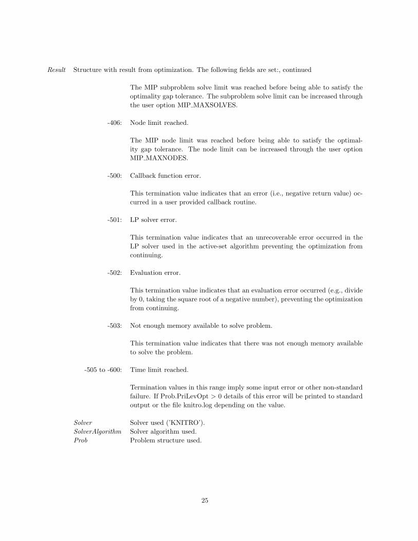
The MIP subproblem solve limit was reached before being able to satisfy theoptimality gap tolerance. The subproblem solve limit can be increased throughthe user option MIP MAXSOLVES.

-406: Node limit reached.

The MIP node limit was reached before being able to satisfy the optimal-ity gap tolerance. The node limit can be increased through the user optionMIP MAXNODES.

-500: Callback function error.

This termination value indicates that an error (i.e., negative return value) oc-curred in a user provided callback routine.

-501: LP solver error.

This termination value indicates that an unrecoverable error occurred in theLP solver used in the active-set algorithm preventing the optimization fromcontinuing.

-502: Evaluation error.

This termination value indicates that an evaluation error occurred (e.g., divideby 0, taking the square root of a negative number), preventing the optimizationfrom continuing.

-503: Not enough memory available to solve problem.

This termination value indicates that there was not enough memory availableto solve the problem.

-505 to -600: Time limit reached.

Termination values in this range imply some input error or other non-standardfailure. If Prob.PriLevOpt > 0 details of this error will be printed to standardoutput or the file knitro.log depending on the value.

Solver Solver used (’KNITRO’).SolverAlgorithm Solver algorithm used.Prob Problem structure used.

25

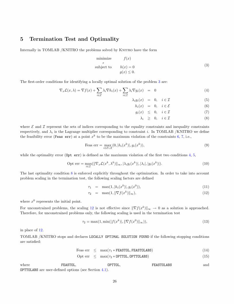
5 Termination Test and Optimality

Internally in TOMLAB /KNITRO the problems solved by Knitro have the form

minimizex

f(x)

subject to h(x) = 0g(x) ≤ 0.

(3)

The first-order conditions for identifying a locally optimal solution of the problem 3 are:

∇xL(x, λ) = ∇f(x) +∑i∈E

λi∇hi(x) +∑i∈I

λi∇gi(x) = 0 (4)

λigi(x) = 0, i ∈ I (5)

hi(x) = 0, i ∈ E (6)

gi(x) ≤ 0, i ∈ I (7)

λi ≥ 0, i ∈ I (8)

where E and I represent the sets of indices corresponding to the equality constraints and inequality constraintsrespectively, and λi is the Lagrange multiplier corresponding to constraint i. In TOMLAB /KNITRO we definethe feasibility error (Feas err) at a point xk to be the maximum violation of the constraints 6, 7, i.e.,

Feas err = maxi∈E∪I

(0, |hi(xk)|, gi(xk)), (9)

while the optimality error (Opt err) is defined as the maximum violation of the first two conditions 4, 5,

Opt err = maxi∈I

(‖∇xL(xk, λk)‖∞, |λigi(xk)|, |λi|, |gi(xk)|). (10)

The last optimality condition 8 is enforced explicitly throughout the optimization. In order to take into accountproblem scaling in the termination test, the following scaling factors are defined

τ1 = max(1, |hi(x0)|, gi(x0)), (11)

τ2 = max(1, ‖∇f(xk)‖∞), (12)

where x0 represents the initial point.

For unconstrained problems, the scaling 12 is not effective since ‖∇f(xk)‖∞ → 0 as a solution is approached.Therefore, for unconstrained problems only, the following scaling is used in the termination test

τ2 = max(1,min(|f(xk)|, ‖∇f(x0)‖∞)), (13)

in place of 12.

TOMLAB /KNITRO stops and declares LOCALLY OPTIMAL SOLUTION FOUND if the following stopping conditionsare satisfied:

Feas err ≤ max(τ1 ∗ FEASTOL, FEASTOLABS) (14)

Opt err ≤ max(τ2 ∗ OPTTOL, OPTTOLABS) (15)

where FEASTOL, OPTTOL, FEASTOLABS andOPTTOLABS are user-defined options (see Section 4.1).

26

This stopping test is designed to give the user much flexibility in deciding when the solution returned by TOMLAB/KNITRO is accurate enough. One can use a purely scaled stopping test (which is the recommended default option)by setting FEASTOLABS and OPTTOLABS equal to 0.0e0. Likewise, an absolute stopping test can be enforced bysetting FEASTOL and OPTTOL equal to 0.0e0.

Unbounded problems

Since by default, TOMLAB /KNITRO uses a relative/scaled stopping test it is possible for the optimality con-ditions to be satisfied for an unbounded problem. For example, if τ2 → ∞ while the optimality error 10 staysbounded, condition 15 will eventually be satisfied for some OPTTOL>0. If you suspect that your problem may beunbounded, using an absolute stopping test will allow TOMLAB /KNITRO to detect this.

27

6 TOMLAB /KNITRO Output

If PriLevOpt=0 then all printing of output is suppressed. For the default printing output level (PriLevOpt=2) thefollowing information is given:

Nondefault Options:

This output lists all user options (see Section 4.1) which are different from their default values. If nothing is listedin this section then all user options are set to their default values.

Problem Characteristics:

The output begins with a descriptionoftheproblemcharacteristics.

Iteration Information:

A major iteration, in the context of Knitro, is defined as a step which generates a new solution estimate (i.e., asuccessful step). A minor iteration is one which generates a trial step (which may either be accepted or rejected).After the problem characteristic information there are columns of data reflecting information about each iterationof the run. Below is a description of the values contained under each column header:

Iter: Iteration number.

Res: The step result. The values in this column indicate whether or not the step attempted during theiteration was accepted (Acc) or rejected (Rej) by the merit function. If the step was rejected, thesolution estimate was not updated. (This information is only printed if PriLevOpt>3).

Objective: Gives the value of the objective function at the trial iterate.

Feas err: Gives a measure of the feasibility violation at the trial iterate.

Opt Err: Gives a measure of the violation of the Karush-Kuhn-Tucker (KKT) (first-order) optimality conditions(not including feasibility).

||Step||: The 2-norm length of the step (i.e., the distance between the trial iterate and the old iterate).

CG its: The number of Projected Conjugate Gradient (CG) iterations required to compute the step.

If PriLevOpt=2, information is printed every 10 major iterations. IfPriLevOpt=3 information is printed at each major iteration. If PriLevOpt=4 in addition to printing iterationinformation on all the major iterations (i.e., accepted steps), the same information will be printed on all minoriterations as well.

Termination Message: At the end of the run a termination message is printed indicating whether or not theoptimal solution was found and if not, why the code terminated. See 4.1 for a list of possibletermination messages and a description of their meaning and corresponding return value.

Final Statistics:

Following the termination message some final statistics on the run are printed. Both relative and absolute errorvalues are printed.

28

Solution Vector/Constraints:

If PriLevOpt=5, the values of the solution vector are printed after the final statistics. If PriLevOpt=6, the finalconstraint values are also printed before the solution vector and the values of the Lagrange multipliers (or dualvariables) are printed next to their corresponding constraint or bound.

29

7 Algorithm Options

7.1 Automatic

By default, Knitro will automatically try to choose the best optimizer for the given problem based on the problemcharacteristics.

7.2 Interior/Direct

If the Hessian of the Lagrangian is ill-conditioned or the problem does not have a large-dense Hessian, it may beadvisable to compute a step by directly factoring the KKT (primal-dual) matrix rather than using an iterativeapproach to solve this system. Knitro offers the Interior/Direct optimizer which allows the algorithm to takedirect steps by setting ALG=1. This option will try to take a direct step at each iteration and will only fall back onthe iterative step if the direct step is suspected to be of poor quality, or if negative curvature is detected.

Using the Interior/Direct optimizer may result in substantial improvements over Interior/CG when the problemis ill-conditioned (as evidenced by Interior/CG taking a large number of Conjugate Gradient iterations). We en-courage the user to try both options as it is difficult to predict in advance which one will be more effective on agiven problem.

NOTE: Since the Interior/Direct algorithm in Knitro requires the explicit storage of a Hessian matrix, thisversion can only be used with Hessian options, HESSOPT=1, 2, 3 or 6. It may not be used with Hessian options,HESSOPT=4 or 5, which only provide Hessian-vector products.

7.3 Interior/CG

Since Knitro was designed with the idea of solving large problems, the Interior/CG optimizer in Knitro offersan iterative Conjugate Gradient approach to compute the step at each iteration. This approach has proven to beefficient in most cases and allows Knitro to handle problems with large, dense Hessians, since it does not requirefactorization of the Hessian matrix. The Interior/CG algorithm can be chosen by setting ALG=2. It can use any ofthe Hessian options as well as the feasible option.

7.4 Active

Knitro 4.0 introduces a new active-set Sequential Linear-Quadratic Programing (SLQP) optimizer. This opti-mizer is particular advantageous when “warm starting” (i.e., when the user can provide a good initial solutionestimate, for example, when solving a sequence of closely related problems). This algorithm is also the preferredalgorithm for detecting infeasible problems quickly. The Active algorithm can be chosen by setting ALG=3. It canuse any of the Hessian options.

30

8 Other special features

This section describes in more detail some of the most important features of Knitro and provides some guidanceon which features to use so that Knitro runs most efficiently for the problem at hand.

8.1 First derivative and gradient check options

The default version of Knitro assumes that the user can provide exact first derivatives to compute the objectivefunction gradient (in dense format) and constraint gradients (in sparse form). It is highly recommended thatthe user provide at least exact first derivatives if at all possible, since using first derivative approximations mayseriously degrade the performance of the code and the likelihood of converging to a solution. However, if this isnot possible or desirable the following first derivative approximation options may be used.

Forward finite-differencesThis option uses a forward finite-difference approximation of the objective and constraint gradients. The cost ofcomputing this approximation is n function evaluations where n is the number of variables. This option can beinvoked by choosing GRADOPT=2.

Centered finite-differencesThis option uses a centered finite-difference approximation of the objective and constraint gradients. The cost ofcomputing this approximation is 2n function evaluations where n is the number of variables. This option can beinvoked by choosing GRADOPT=3. The centered finite-difference approximation may often be more accurate thanthe forward finite-difference approximation. However, it is more expensive since it requires twice as many functionevaluations to compute.

Gradient ChecksIf the user is supplying a routine for computing exact gradients, but would like to compare these gradients withfinite-difference gradient approximations as an error check this can easily be done in Knitro. To perform a gradientcheck with forward finite-differences set GRADOPT=4, and to perform a gradient check with centered finite-differencesset GRADOPT=5.

8.2 Second derivative options

The default version of Knitro assumes that the user can provide exact second derivatives to compute the Hessianof the Lagrangian function. If the user is able to do so and the cost of computing the second derivatives is notoverly expensive, it is highly recommended to provide exact second derivatives. However, Knitro also offers otheroptions which are described in detail below.

(Dense) Quasi-Newton BFGSThe quasi-Newton BFGS option uses gradient information to compute a symmetric, positive-definite approximationto the Hessian matrix. Typically this method requires more iterations to converge than the exact Hessian version.However, since it is only computing gradients rather than Hessians, this approach may be more efficient in somecases. This option stores a dense quasi-Newton Hessian approximation so it is only recommended for small tomedium problems (n < 1000). The quasi-Newton BFGS option can be chosen by setting options value HESSOPT=2.

31

(Dense) Quasi-Newton SR1As with the BFGS approach, the quasi-Newton SR1 approach builds an approximate Hessian using gradientinformation. However, unlike the BFGS approximation, the SR1 Hessian approximation is not restricted to bepositive-definite. Therefore the quasi-Newton SR1 approximation may be a better approach, compared to theBFGS method, if there is a lot of negative curvature in the problem since it may be able to maintain a betterapproximation to the true Hessian in this case. The quasi-Newton SR1 approximation maintains a dense Hessianapproximation and so is only recommended for small to medium problems (n < 1000). The quasi-Newton SR1option can be chosen by setting options value HESSOPT=3.

Finite-difference Hessian-vector product optionIf the problem is large and gradient evaluations are not the dominate cost, then Knitro can internally computeHessian-vector products using finite-differences. Each Hessian-vector product in this case requires one additionalgradient evaluation. This option can be chosen by setting options value HESSOPT=4. This option is generally onlyrecommended if the exact gradients are provided.

NOTE: This option may not be used when ALG=1.

Exact Hessian-vector productsIn some cases the user may have a large, dense Hessian which makes it impractical to store or work with theHessian directly, but the user may be able to provide a routine for evaluating exact Hessian-vector products.Knitro provides the user with this option. This option can be chosen by setting options value HESSOPT=5.

NOTE: This option may not be used when ALG=1.

Limited-memory Quasi-Newton BFGSThe limited-memory quasi-Newton BFGS option is similar to the dense quasi-Newton BFGS option describedabove. However, it is better suited for large-scale problems since, instead of storing a dense Hessian approximation,it only stores a limited number of gradient vectors used to approximate the Hessian. The number of gradient vectorsused to approximate the Hessian is controlled by user option LMSIZE which must be between 1 and 100 (10 is thedefault). A larger value of LMSIZE may result in a more accurate, but also more expensive, Hessian approximation.A smaller value may give a less accurate, but faster, Hessian approximation. When using the limited memoryBFGS approach it is recommended to experiment with different values of this parameter. In general, the limited-memory BFGS option requires more iterations to converge than the dense quasi- Newton BFGS approach, but willbe much more efficient on large-scale problems. This option can be chosen by setting options value HESSOPT=6.

8.3 Feasible version

Knitro offers the user the option of forcing intermediate iterates to stay feasible with respect to the inequalityconstraints (it does not enforce feasibility with respect to the equality constraints however). Given an initial pointwhich is sufficiently feasible with respect to all inequality constraints and selecting FEASIBLE = 1, forces all theiterates to strictly satisfy the inequality constraints throughout the solution process. For the feasible mode tobecome active the iterate x must satisfy

cl + tol ≤ c(x) ≤ cu− tol (16)

for all inequality constraints (i.e., for cl 6= cu). The tolerance tol > 0 by which an iterate must be strictly feasiblefor entering the feasible mode is determined by the parameter FEASMODETOL which is 1.0e-4 by default. If the

32

initial point does not satisfy 16 then the default infeasible version of Knitro will run until it obtains a pointwhich is sufficiently feasible with respect to all the inequality constraints. At this point it will switch to thefeasible version of Knitro and all subsequent iterates will be forced to satisfy the inequality constraints.

NOTE: This option may only be used when ALG=1 or 2.

8.4 Honor Bounds

By default Knitro does not enforce that the simple bounds on the variables 1 are satisfied throughout theoptimization process. Rather, satisfaction of these bounds is only enforced at the solution. In some applications,however, the user may want to enforce that the initial point and all intermediate iterates satisfy the boundsxL ≤ x ≤ xU . This can be enforced by setting HONORBNDS=1.

8.5 Crossover

Interior point (or barrier) methods are a powerful tool for solving large-scale optimization problems. However, onedrawback of these methods, in contrast to active-set methods, is that they do not always provide a clear picture ofwhich constraints are active at the solution and in general they return a less exact solution and less exact sensitivityinformation. For this reason, Knitro offers a crossover feature in which the interior-point method switches to theactive-set method at the interior-point solution estimate, in order to try to “clean up” the solution and providemore exact sensitivity and active-set information.

The crossover procedure is controlled by the MAXCROSSIT user option. If this parameter is greater than 0, thenKnitro will attempt to perform MAXCROSSIT active-set crossover iterations after the interior-point method hasfinished, to see if it can provide a more exact solution. This can be viewed as a form of post-processing. IfMAXCROSSIT<=0, then no crossover iterations are attempted. By default, no crossover iterations are performed.

The crossover procedure will not always succeed in obtaining a more exact solution compared with the interior-pointsolution. If crossover is unable to improve the solution within MAXCROSSIT crossover iterations, then it will restorethe interior-point solution estimate and terminate. IfPriLevOpt>1, Knitro will print a message indicating that it was unable to improve the solution. For exam-ple, if MAXCROSSIT=3, and the crossover procedure did not succeed within 3 iterations, the message will read:

Crossover mode unable to improve solution within 3 iterations.

In this case, you may want to increase the value of MAXCROSSIT and try again. If it appears that the crossoverprocedure will not succeed, no matter how many iterations are tried, then a message of the form

Crossover mode unable to improve solution.

will be printed.

The extra cost of performing crossover is problem dependent. In most small or medium scale problems, thecrossover cost should be a small fraction of the total solve cost. In these cases it may be worth using the crossoverprocedure to obtain a more exact solution. On some large scale or difficult degenerate problems, however, the costof performing crossover may be significant. It is recommended to experiment with this option to see whether theimprovement in the exactness of the solution is worth the additional cost.

33

8.6 Multi-start

Nonlinear optimization problems are often nonconvex due to the objective function, constraint functions, or both.When this is true, there may be many points that satisfy the local optimality conditions described in section 5.Default Knitro behavior is to return the first locally optimal point found. Knitro offers a simple multi-startfeature that searches for a better optimal point by restarting Knitro from different initial points. The feature isenabled by setting MSENABLE=1.

The multi-start procedure generates new start points by randomly selecting x components that satisfy the variablebounds. The number of start points to try is specified with the option MSMAXSOLVES. Knitro finds a localoptimum from each start point using the same problem definition and user options. The solution returned is thelocal optimum with the best objective function value. If PriLevOpt is greater than 3, then Knitro prints detailsof each local optimum.

The multi-start option is convenient for conducting a simple search for a better solution point. It can also saveexecution and memory overhead by internally managing the solve process from successive start points.

In most cases the user would like to obtain the global optimum; that is, the local optimum with the very bestobjective function value. Knitro cannot guarantee that mult-start will find the global optimum. The probabilityof finding a better point improves if more start points are tried, but so does the execution time. Search time canbe improved if the variable bounds are made as tight as possible. Minimally, all variables need to be given finiteupper and lower bounds.

8.7 Solving Systems of Nonlinear Equations

Knitro is quite effective at solving systems of nonlinear equations. To solve a square system of nonlinear equationsusing Knitro one should specify the nonlinear equations using clsAssign in TOMLAB. The same applies for leastsquares problems described below.

8.8 Solving Least Squares Problems

There are two ways of using Knitro for solving problems in which the objective function is a sum of squares ofthe form

f(x) = 12

∑qj=1 rj(x)2.

If the value of the objective function at the solution is not close to zero (the large residual case), the least squaresstructure of f can be ignored and the problem can be solved as any other optimization problem. Any of theKnitro options can be used.

On the other hand, if the optimal objective function value is expected to be small (small residual case) thenKnitro can implement the Gauss-Newton or Levenberg-Marquardt methods which only require first derivativesof the residual functions, rj(x), and yet converge rapidly. To do so, the user need only define the Hessian of f tobe

∇2f(x) = J(x)TJ(x),

where

J(x) =[∂rj∂xi

]j = 1, 2, . . . , qi = 1, 2, . . . , n

.

34

The actual Hessian is given by

∇2f(x) = J(x)TJ(x) +q∑

j=1

rj(x)∇2rj(x);

the Gauss-Newton and Levenberg-Marquardt approaches consist of ignoring the last term in the Hessian.

Knitro will behave like a Gauss-Newton method by setting ALG=1, and will be very similar to the classicalLevenberg-Marquardt method when ALG=2.

8.9 Mathematical programs with equilibrium constraints (MPECs)

A mathematical program with equilibrium (or complementarity) constraints (also know as an MPEC or MPCC) isan optimization problem which contains a particular type of constraint referred to as a complementarity constraint.A complementarity constraint is a constraint which enforces that two variables are complementary to each other,i.e., the variables x1 and x2 are complementary if the following conditions hold

x1 × x2 = 0, x1 ≥ 0, x2 ≥ 0. (17)

The condition above, is sometimes expressed more compactly as

0 ≤ x1 ⊥ x2 ≥ 0.

One could also have more generally, that a particular constraint is complementary to another constraint or aconstraint is complementary to a variable. However, by adding slack variables, a complementarity constraintcan always be expressed as two variables complementary to each other, and Knitro requires that you expresscomplementarity constraints in this form. For example, if you have two constraints c1(x) and c2(x) which arecomplementary

c1(x)× c2(x) = 0, c1(x) ≥ 0, c2(x) ≥ 0,

you can re-write this as two equality constraints and two complementary variables, s1 and s2 as follows:

s1 = c1(x) (18)

s2 = c2(x) (19)

s1 × s2 = 0, s1 ≥ 0, s2 ≥ 0. (20)

Intuitively, a complementarity constraint is a way to model a constraint which is combinatorial in nature since, forexample, the conditions in 17 imply that either x1 or x2 must be 0 (both may be 0 as well). Without special care,these type of constraints may cause problems for nonlinear optimization solvers because problems which containthese types of constraints fail to satisfy constraint qualifications which are often assumed in the theory and designof algorithms for nonlinear optimization. For this, reason we provide a special interface in Knitro for specifyingcomplementarity constraints. In this way, Knitro can recognize these constraints and apply some special care tothem internally.

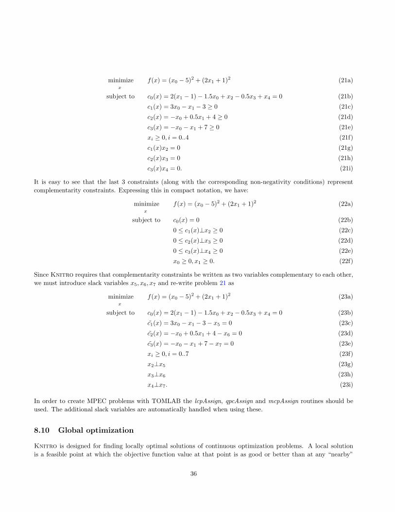
Assume we want to solve the following MPEC with Knitro.

35

minimizex

f(x) = (x0 − 5)2 + (2x1 + 1)2 (21a)

subject to c0(x) = 2(x1 − 1)− 1.5x0 + x2 − 0.5x3 + x4 = 0 (21b)

c1(x) = 3x0 − x1 − 3 ≥ 0 (21c)

c2(x) = −x0 + 0.5x1 + 4 ≥ 0 (21d)

c3(x) = −x0 − x1 + 7 ≥ 0 (21e)

xi ≥ 0, i = 0..4 (21f)

c1(x)x2 = 0 (21g)

c2(x)x3 = 0 (21h)

c3(x)x4 = 0. (21i)

It is easy to see that the last 3 constraints (along with the corresponding non-negativity conditions) representcomplementarity constraints. Expressing this in compact notation, we have:

minimizex

f(x) = (x0 − 5)2 + (2x1 + 1)2 (22a)

subject to c0(x) = 0 (22b)

0 ≤ c1(x)⊥x2 ≥ 0 (22c)

0 ≤ c2(x)⊥x3 ≥ 0 (22d)

0 ≤ c3(x)⊥x4 ≥ 0 (22e)

x0 ≥ 0, x1 ≥ 0. (22f)

Since Knitro requires that complementarity constraints be written as two variables complementary to each other,we must introduce slack variables x5, x6, x7 and re-write problem 21 as

minimizex

f(x) = (x0 − 5)2 + (2x1 + 1)2 (23a)

subject to c0(x) = 2(x1 − 1)− 1.5x0 + x2 − 0.5x3 + x4 = 0 (23b)

c1(x) = 3x0 − x1 − 3− x5 = 0 (23c)

c2(x) = −x0 + 0.5x1 + 4− x6 = 0 (23d)

c3(x) = −x0 − x1 + 7− x7 = 0 (23e)

xi ≥ 0, i = 0..7 (23f)

x2⊥x5 (23g)

x3⊥x6 (23h)

x4⊥x7. (23i)

In order to create MPEC problems with TOMLAB the lcpAssign, qpcAssign and mcpAssign routines should beused. The additional slack variables are automatically handled when using these.

8.10 Global optimization

Knitro is designed for finding locally optimal solutions of continuous optimization problems. A local solutionis a feasible point at which the objective function value at that point is as good or better than at any “nearby”

36

feasible point. A globally optimal solution is one which gives the best (i.e., lowest if minimizing) value of theobjective function out of all feasible points. If the problem is convex all locally optimal solutions are also globallyoptimal solutions. The ability to guarantee convergence to the global solution on large-scale nonconvex problemsis a nearly impossible task on most problems unless the problem has some special structure or the person modelingthe problem has some special knowledge about the geometry of the problem. Even finding local solutions tolarge-scale, nonlinear, nonconvex problems is quite challenging.

Although Knitro is unable to guarantee convergence to global solutions it does provide a multi-start heuristicwhich attempts to find multiple local solutions in the hopes of locating the global solution. See section 8.6 forinformation on trying to find the globally optimal solution using the Knitro multi-start feature.

37

Documents

USER'S GUIDE FOR TOMLAB /KNITRO v5 - MATLAB OPTIMIZATION and .NET