User s Manual - i-Tree · i-Tree Species Selector is a free-standing utility designed to help urban foresters ... Phase I: Creating a New Project ... Digital Elevation Model

Hydro

User’s Manual

10.28.2016 v. 5.1

i-Tree is a cooperative initiative

About i-Tree i-Tree is a state-of-the-art, peer-reviewed software suite from the USDA Forest Service that provides urban and community forestry analysis and benefits assessment tools. The i-Tree tools help communities of all sizes to strengthen their urban forest management and advocacy efforts by quantifying the environmental services that trees provide and assessing the structure of the urban forest. i-Tree has been used by communities, non-profit organizations, consultants, volunteers, and students to report on the urban forest at all scales from individual trees to parcels, neighborhoods, cities, and entire states. By understanding the local, tangible ecosystem services that trees provide, i-Tree users can link urban forest management activities with environmental quality and community livability. Whether your interest is a single tree or an entire forest, i-Tree provides baseline data that you can use to demonstrate value and set priorities for more effective decision-making. Developed by USDA Forest Service and numerous cooperators, i-Tree is in the public domain and available by request through the i-Tree website (www.itreetools.org).The Forest Service, Davey Tree Expert Company, the Arbor Day Foundation, Society of Municipal Arborists, the International Society of Arboriculture, and Casey Trees have entered into a cooperative partnership to further develop, disseminate, and provide technical support for the suite.

i-Tree Products

The i-Tree software suite v. 5 includes the following urban forest analysis tools and utility programs. i-Tree Eco provides a broad picture of the entire urban forest. It is designed to use field data from randomly located plots throughout a community along with local hourly air pollution and meteorological data to quantify urban forest structure, environmental effects, and value to communities. i-Tree Streets focuses on the ecosystem services and structure of a municipality’s street tree population. It makes use of a sample or complete inventory to quantify and put a dollar value on the trees’ annual environmental and aesthetic benefits, including energy conservation, air quality improvement, carbon dioxide reduction, stormwater control, and property value increases. i-Tree Hydro is the first vegetation-specific urban hydrology model. It is designed to model the effects of changes in urban tree cover and impervious surfaces on the hydrological cycle, including streamflow and water quality, for watershed and non-watershed areas.

i-Tree Vue allows you to make use of the freely available National Land Cover Database (NLCD) satellite-based imagery to assess your community’s land cover, including tree canopy, and some of the ecosystem services provided by your current urban forest. The effects of planting scenarios on future benefits can also be modeled. i-Tree Species Selector is a free-standing utility designed to help urban foresters select the most appropriate tree species based on environmental function and geographic area. i-Tree Storm helps you to assess widespread community damage in a simple, credible, and efficient manner immediately after a severe storm. It is adaptable to various community types and sizes and provides information on the time and funds needed to mitigate storm damage. i-Tree Design is a simple online tool that provides a platform for assessments of individual trees at the parcel level. This tool links to Google Maps and allows you to see how tree selection, tree size, and placement around your home affects energy use and other benefits. This tool is in the early stages of development; more sophisticated options will be available in future versions. i-Tree Canopy offers a quick and easy way to produce a statistically valid estimate of land cover types (e.g., tree cover) using aerial images available in Google Maps. The data can be used by urban forest managers to estimate tree canopy cover, set canopy goals, and track success; and to estimate inputs for use in i-Tree Hydro and elsewhere where land cover data are needed.

Disclaimer

The use of trade, firm, or corporation names in this publication is solely for the information and convenience of the reader. Such use does not constitute an official endorsement or approval by the U.S. Department of Agriculture or the Forest Service of any product or service to the exclusion of others that may be suitable. The software distributed under the label “i-Tree Software Suite v. 5” is provided without warranty of any kind. Its use is governed by the End User License Agreement (EULA) to which the user agrees before installation.

Feedback

The i-Tree Development Team actively seeks feedback on any component of the project: the software suite itself, the manuals, or the process of development, dissemination, support, and refinement. Please send comments through any of the means listed on the i-Tree support page: www.itreetools.org/support.

http://www.itreetools.org/support

Acknowledgments

i-Tree

Components of the i-Tree software suite have been developed over the last few decades by the USDA Forest Service and numerous cooperators. Support for the development and release of i-Tree v. 5 has come from USDA Forest Service Research, State and Private Forestry, and their cooperators through the i-Tree Cooperative Partnership of Davey Tree Expert Company, the Arbor Day Foundation, Society of Municipal Arborists, the International Society of Arboriculture, and Casey Trees.

i-Tree Hydro The i-Tree Hydro model was originally developed by Drs. Jun Wang SUNY College of Environmental Science and Forestry (SUNY-ESF), Ted Endreny (SUNY-ESF), and David J. Nowak, USDA Forest Service, Northern Research Station (USFS-NRS). The model code has been improved and integrated within i-Tree based on the work of Megan Kerr (Davey Institute), Yang Yang (SUNY-ESF), Sanyam Chaudhary (Syracuse University), Rahul Kumbhar (Syracuse University), Yu Chen (Syracuse University), Thomas Taggart (SUNY-ESF), Shannon Conley (SUNY-ESF), Yu Chen (Syracuse University), Pallavi Iyengar (Syracuse University), Jeevitha Royapathi (Syracuse University), Isira Samarasekera (Syracuse University), Vamsi Kodali (Syracuse University), and Sunit Vijayvargiya (Syracuse University). Topographic Index calculations have been improved with algorithms developed for WhiteBox GAT (Lindsay, 2016) with permission by its creator John Lindsay, PhD (University of Guelph). Many other individuals have contributed to the design, development, testing process, and help text including Andrew Lee (SUNY-ESF), Robert Hoehn (USDA Forest Service), Tian Zhou (SUNY-ESF), Scott Maco (Davey Institute), Mike Binkley (Davey Institute), Lianghu Tian (Davey Institute), David Ellingsworth (Davey Institute), Alexis Ellis (Davey Institute), Allison Bodine (Davey Institute), Dr. Jim Fawcett (Syracuse University), Emily Stephan (SUNY-ESF), and Robert Coville (Davey Institute). The original manual was written & designed by Kelaine Vargas (Davey Institute), and it has been updated by Robert Coville (Davey Institute).

Table of Contents Introduction .............................................................................................................................. 1

Overview .................................................................................................................................................. 1

About This Manual ................................................................................................................................. 2

Installation ................................................................................................................................ 4

System Requirements ........................................................................................................................... 4

Installation ............................................................................................................................................... 4

Exploring i-Tree Hydro with the Sample Project ................................................................................ 5

Phase I: Creating a New Project.............................................................................................. 6

Entering the Project Area Information ................................................................................................. 6

Phase II: Entering Model Parameters ..................................................................................... 9

Entering the Land Cover Parameters.................................................................................................. 9

Entering the Hydrological Parameters .............................................................................................. 10

Calibration process overview .......................................................................................................... 11

Calibrating the model ....................................................................................................................... 11

Comparing the calibration results .................................................................................................. 13

Saving/loading hydrological parameters for/from other i-Tree Hydro projects ....................... 13

Defining the Alternative Case ............................................................................................................. 14

Phase III: Exploring i-Tree Hydro Outputs ............................................................................15

Running the i-Tree Hydro Model ........................................................................................................ 15

Executive Summary ............................................................................................................................. 15

Graphs and Tables............................................................................................................................... 16

Water volume .................................................................................................................................... 17

Pollution estimates ........................................................................................................................... 18

Water flow .......................................................................................................................................... 19

Water pollution .................................................................................................................................. 21

DEM 2D/3D Visualization .................................................................................................................... 22

Calibration Comparison ....................................................................................................................... 23

Extended Outputs for Advanced Users ............................................................................................ 24

Enabling extended outputs & configuring your working directory ............................................. 24

Accessing & understanding extended outputs of a specific Hydro run .................................... 25

Additional Information ............................................................................................................28

Choosing Your Watershed and Gaging Station .............................................................................. 28

Tools for choosing the best stream gage station and watershed: ............................................ 28

Gathering Data ..................................................................................................................................... 31

Basic watershed characteristics ..................................................................................................... 32

Digital Elevation Model (DEM) ....................................................................................................... 32

Topographic Index (TI) .................................................................................................................... 32

Observed streamflow ....................................................................................................................... 33

Weather station ................................................................................................................................. 34

Land cover parameters ................................................................................................................... 36

Leaf Area Index (LAI) ....................................................................................................................... 37

Directly Connected Impervious Area (DCIA) ............................................................................... 37

Calibrating the Model Manually .......................................................................................................... 41

Appendix 1: Creating a Watershed Digital Elevation Model ................................................43

Downloading DEM Data from USGS ................................................................................................ 43

Working with ArcGIS ............................................................................................................................ 46

Appendix 2: Topographic Index Data ....................................................................................51

Appendix 3: Calculating Pollution Load ................................................................................52

Appendix 4: International Support .........................................................................................56

Appendix 5: Glossary .............................................................................................................58

Appendix 6: Additional Resources ........................................................................................63

References ..............................................................................................................................66

1

Introduction i-Tree Hydro is a simulation tool that analyzes how land cover influences the hydrological cycle, including the volume and quality of runoff. It can analyze historical or future hydrological events and allow the user to contrast runoff volume and quality from existing land cover (referred to as the Base Case) with runoff from contrasting land cover (referred to as the Alternative Case). The i-Tree Hydro model differs from other i-Tree products in the following ways:

• The model simulation area is selected from a pre-loaded Topographic Index (TI) files for 1000s of watersheds and places, or is loaded into the program as a Digital Elevation Model (DEM) file or as a TI file. It is not hand-delineated in the program by the user. If you are interested in a watershed, you can use either a DEM or pre-loaded TI file. If you are interested in a US state, county, city or other US Census place, you would use a pre-loaded TI file. For other areas without pre-loaded elevation data, you would use a DEM file.

• The model simulation can be run in calibration mode or non-calibration mode.

For calibration mode, the user loads observed streamflow data from a gaging station and the model will identify an optimal set of hydrological parameters to try and match the observed data. Streamflow gage data can be found for thousands of watershed areas. For non-calibration runs, the user can employ previously calibrated parameters or independently set the land cover and hydrological parameter values by adjusting the default values that the model provides.

Any user with reasonable knowledge of the project area can use pre-loaded elevation data (where available) and run i-Tree Hydro in non-calibration mode with suggested hydrological parameters and the weather station information included in i-Tree Hydro. However, more confidence in model parameters comes with model calibration.

Overview

i-Tree Hydro models the hydrological cycle and estimates runoff volume and water quality using inputs of elevation, land cover, weather, and various model parameters. The user can explore how the outputs change with changes in model inputs such as tree and impervious cover. Some additional information on inputs:

• For elevation data – to simulate a standard area such as USGS gage watersheds or US census places, the model is best suited to use pre-loaded Topographic Index (TI) data. For other unique user-defined areas, the model is best suited to use free Digital Elevation Model (DEM) data.

2

• For land cover data – percent tree cover, shrub cover, impervious surface, and other cover types are needed. These values can be obtained using updated National Land Cover Data (NLCD) from the USGS. You can also derive these values from i-Tree Canopy, available online at www.itreetools.org.

• For weather – the model includes weather data from 2005-2012. With some

formatting, you can also load your own weather files.

• For model parameters – the model provides Suggested Default Values that can be modified to better represent the specific analysis area. For soils data, the user can change the default values to represent their area.

• i-Tree Hydro can be run for the Base Case to assess current conditions in your

project area. To contrast how land cover changes affect the runoff volume and water quality, an Alternative Case can be run. To save time, both Base Case and Alternative Case can be specified at the outset. The Alternative Case can be changed and the model re-run at any time.

You can get a preview at File > Open the Sample Project. When you are ready, get started with File > New Project. For more information on the methodology that underlies i-Tree Hydro, visit

www.itreetools.org > Resources > Archives > i-Tree Hydro Resources

About This Manual

This manual provides information needed to conduct an i-Tree Hydro project. After installing the software and exploring a sample project, we’ll move on to three general project phases: Phase I: Creating a New Project. In this section, we’ll provide an overview of the steps necessary to create a new project, input your Base Case data, and calibrate the model. Phase II: Entering Model Parameters. In this section, we’ll explain how to adjust land cover, hydrological, and Alternative Case parameters. Phase III: Exploring Model Outputs. In the third phase, we get to the crux of i-Tree Hydro – running the model, viewing the executive summary and other model outputs, and interpreting the results.

http://www.itreetools.org/


3

Additional Information. This section explains some of the more challenging steps involved with running i-Tree Hydro, such as choosing your watershed, gathering input data, and calibrating the model. The following appendices provide further detail on running i-Tree Hydro: Appendix 1: Creating a Watershed Digital Elevation Model. This appendix describes the necessary tools and steps involved in creating a Digital Elevation Model (DEM) for a watershed using ArcGIS. Appendix 2: Topographic Index Data. This appendix provides an overview of the Topographic Index (TI) data that can be used in place of a DEM. Appendix 3: Calculating Pollution Load. This appendix describes the methodology associated with estimating how changes in hydrology affect water pollutant levels. Appendix 4: International Support. This appendix includes a brief overview of the raw data required to run i-Tree Hydro outside of the United States. Appendix 5: Glossary. This appendix contains definitions of many of the terms used throughout this manual and in the i-Tree Hydro program. Appendix 6: Additional Resources. This appendix instructs the reader on where to find background information, data, and help that is not included in this manual or the i-Tree Graphical User Interface (GUI).

4

Installation

System Requirements

Minimum hardware:

• 1.6 GHz or faster processor • 1024 MB or more of available RAM • Hard drive with at least 500 MB free space • Monitor with resolution of at least 1024 x 768

Software:

• Windows 7 or higher OS • .NET 4.0 framework or newer (included in i-Tree installation) • Adobe Reader 9.0 or newer

Installation

To install i-Tree Hydro:

1. Visit www.itreetools.org to download the software or insert an i-Tree Installation CD into your CD-ROM drive.

2. Follow the on-screen instructions to run i-Tree setup.exe. This may take several

minutes depending on which files need to be installed.

3. Follow the Installation Wizard instructions to complete the installation (default location recommended).

You can check for the latest updates at any time in i-Tree Hydro by clicking Help > Check for Updates.


5

Exploring i-Tree Hydro with the Sample Project

Now that you’ve installed i-Tree Hydro, you would probably like to see a little of what the software can do. To allow you to explore the program, we’ve included a sample project based on the Rock Creek watershed near Washington, DC.

1. You begin by opening i-Tree Hydro using your computer’s Start menu > (All) Programs > i-Tree > Hydro.

2. You will find the sample project under File > Open the Sample Project.

a. Under Step 1) Project Area Information, you can review the input data

fields. Additional input parameters can also be viewed by going through Step 2) Land Cover Parameters or Step 3) Hydrological Parameters.

b. Tree and impervious cover parameters can be adjusted to see how these

changes affect the hydrology of the project area. Click Step 4) Define Alternative Case and make adjustments as desired. On your first exploration into i-Tree Hydro, we recommend leaving these inputs as they are. You can always return and make adjustments.

c. Click Input > 5) Run Hydro Model to run the sample project and calculate

outputs.

d. Under the Output menu, review the graphs and tables that are available for your watershed analysis over various time periods. For example:

• Executive Summary – a three-page summation of basic results.

• Water Volume – estimates of the water flowing out of your project

area.

• Pollutant Estimates – pollutant loads in the water flow.

• Water Flow – tables and graphs showing how water flow and rainfall vary over time.

• Water Pollution – tables and graphs presenting the pollutant load

associated with Base and Alternative Case water flow. We explain all of these steps and outputs in greater detail. For now, feel free to explore and see what’s available.

6

Phase I: Creating a New Project

To begin working with i-Tree Hydro, click your computer’s Start menu > (All) Programs > i-Tree > Hydro.

NOTE: The Additional Information section later in the manual provides directions for choosing your project area, gathering your data, and calibrating the Hydro model. It is meant to supplement the more general directions provided in this section and you may find it beneficial to explore that section before creating a new project.

To start a new project:

1. Click File > New Project. In the Save As window that appears, navigate to the folder that you wish to save your project in.

2. Give your new project a name and click Save.

3. Select a simulate type: watershed or a non-watershed. This affects what pre-loaded areas are available (e.g. cities or watersheds) and whether or not you can input observed streamflow data for auto-calibration of the model. Non-watershed areas are those where water does not drain & discharge to a single outlet. For non-watershed areas, or uncalibrated watersheds, we consider results limited to qualitative comparisons between scenarios.

Now that your new project has been created, it is time to enter your input data and adjust the parameters of the model. As you navigate through each step, you can review the Help text in the right-side panels for more detail about each of the model inputs and parameters. The Help text for each variable appears when you hover over the variable.

Entering the Project Area Information

Begin developing your i-Tree Hydro project by entering the Project Area Information.

1. Open the Step 1) Project Area Information window under the Steps menu. (This window opens automatically when you create a new project.)

2. Enter the Project Location for your watershed or study area. Since watersheds

are not confined to political or parcel boundaries, it is important to choose the state, county, and city in which the greatest portion of your watershed is located. If your city is not listed, choose N/A in the alphabetical listing.

3. Enter the Digital Elevation Model / Topographic Index for your project area. In order to incorporate necessary elevation information, you have a few options:

7

a. If you choose to represent a watershed model simulation area using a digital elevation model (DEM), choose Browse for my own DEM file, navigate to the location where you saved the file, and click Open.

For basic instructions on the process for creating a watershed DEM, see the Additional Information section and .

b. If you choose to represent the model simulation area using a topographic

index (TI), choose Use a Topographic Index.

In the window that appears, you can Browse for my own Topographic Index file if you have prepared your own TI. Navigate to the location where you saved the file and click Open. For basic instructions on the process of creating a TI, see the Additional Information section and Appendix 2: Topographic Index Data. Alternatively, you can choose to Select Topographic Index data from the i-Tree Hydro database. Select the desired TI boundary from the drop-down menus. In the window that appears, navigate to the folder where you saved your project, give the file a name (e.g., TI_data.dat), and click Save.

4. Enter the Basic Watershed Characteristics for your watershed or study area.

a. The Watershed Land Area can be entered in either square kilometers

(km2) or square miles (mi2). To toggle between the two options, simply check or uncheck the box labeled Metric.

b. Choose a Start Date/Time and End Date/Time. These will denote the first

and last recorded time step of the observed streamflow data and the weather station data used in the model run.

If you are using the 2005-2012 data included in i-Tree Hydro, the weather and stream gage data will be filtered by your chosen Start and End Date/Time. If you are loading your own data, make sure you choose appropriate Date/Times that are the same for both data sets. Projects should be limited to three years or fewer, given the intensive amount of processing.

NOTE: The default time period ends on December 30, at time 23:00. The exclusion of the last day of the year, December 31, avoids problems that can arise when converting streamflow and weather data from different time-zones into a standard time-zone.

5. There are three options when it comes to Observed Streamflow Data:

8

a. If you will be using the standard i-Tree Hydro data (available for 2005-2012), click I need to pick a USGS gage from a map and a map of local gaging stations will appear.

To select an appropriate station, you can enter the ID number directly in the ID field or click on the station marker to select it. If you hover over each marker, the station name will appear in the window status bar. After you have selected an appropriate station, click OK. Processing will begin.

b. If you gathered your own data, choose Browse for my own (raw or

processed) stream gauge file, navigate to the location where you saved the file and click Open. See the Additional Information section for details on how to gather and format your own stream gage data.

c. If you would like to conduct an analysis as a non-gaged stream or a non-

watershed area, choose I wish to predict streamflow for a non-gaged stream. This disables auto-calibration to observed streamflow data in Step 3) Hydrological Parameters, and the model will use estimated values instead.

6. Accurate, complete, and nearby weather data is critical for the best i-Tree Hydro

estimates. In order to incorporate Weather Station Data, you have two options:

a. If you will be using the standard i-Tree Hydro data for 2005-2012, click I need to pick a weather station from a map and a map of local weather stations will appear. To select an appropriate station, you can enter the ID number directly in the ID field or click on the station marker to select it. If you hover over each marker, the station name will appear in the window status bar. After you have selected an appropriate station, click OK. Processing will begin.

b. If you gathered and properly formatted your own data, choose Browse for

my own file, navigate to the location where you saved the file, and click Open. See the Additional Information section for details on how to gather and format your own stream gage data.

NOTE: If you would like to save streamflow & weather data that you chose, after exiting Step 1 go to File > Save Weather and Gage Data and choose which type of data file you would like to save (raw or processed stream gage or weather data). Give the data file(s) an appropriate name (e.g., streamgage_data.dat), and click Save.

Once you have finished in this window, click OK to close. It’s a good idea to save your project at this time, so click File > Save Project. Be sure to save your project periodically.

9

NOTE: If you change any of the fields in Step 1) Project Area Information, you must redo streamflow & weather data selection. Changes to these fields require i-Tree Hydro to reprocess streamflow & weather data.

Phase II: Entering Model Parameters

Entering the Land Cover Parameters

To continue developing your i-Tree Hydro project, enter the Land Cover Parameters that describe your project area.

1. Open the Step 2) Land Cover Parameters window under the Steps menu.

2. Enter the Surface Cover Types for your watershed or study area. These parameter values are important as they help describe the land cover conditions of the study area. These parameters describe what is visible at the canopy level. If a tree is planted in a parking lot, the area of the tree’s canopy is converted into percent tree cover. See Figure 1 for a graphical interpretation of this. At this point, Tree Cover will already have been defined as the value set in the Step 1) Project Area Information window, since it was needed for various initial processing steps, such as calculating evapotranspiration, etc. Refer to the Leaf Area Index (LAI)

Leaf Area Index (LAI) is the total leaf area divided by the canopy area. More specifically, it is the ratio of 1-sided surface area of leaves (m) per unit canopy cover (m). LAI is a dimensionless variable describing leaf area density per canopy cover. A way to think about LAI is to imagine drawing a square on the ground under a tree canopy, with sides 1 meter in length. Standing in this 1-meter square area, looking up into the tree canopy, the LAI represents the surface area (1-sided) of the leaves present directly above this 1 meter square area. Typical LAI values range from 1-7, representing 1-7 square meters of leaf area (1-sided) above this 1-meter square area. Leaf area index can be derived from certain i-Tree Eco results. When deriving leaf area index for i-Tree Hydro, it is important keep in mind that leaf area index is the leaf area per unit canopy cover. Some variables in i-Tree Eco describe the density of leaves in a certain strata or land use, or per unit ground cover within the entire project area. The difference is due to what each tool is designed for: in Eco, the interest in leaf area is describing tree canopy in the context of a city, a strata, a land use, etc.; in Hydro, the interest is the properties of tree canopy itself wherever it exists in the project area.

10

Directly Connected Impervious Area (DCIA) section for instructions on calculating DCIA.

3. Enter the Cover Types Beneath Tree Cover for your watershed or study area.

These cover types represent the percentages of pervious and impervious land beneath the tree canopy. If a tree is planted in a parking lot, the area of parking lot underneath the tree’s canopy is converted into percent impervious cover. See Figure 1 for a graphical interpretation of this.

NOTE: In this window, you are describing the entire watershed as best you can. However, to avoid over- or underestimating, total surface cover types and total sub-types should both add up to 100%.

Again, be sure to save your current project periodically.

Fig. 1: Step 2) Land Cover Parameters – depiction of what type of land cover is represented in each sub-step

Entering the Hydrological Parameters

Calibrating your i-Tree Hydro project involves a multi-step process of adjusting model parameters until the modeled streamflow resembles the actual streamflow. i-Tree Hydro features an auto-calibration routine that uses the observed streamflow data from a gaging station to identify the optimal hydrological parameters to fit the observed streamflow data. The user can also manually enter hydrological parameter values by adjusting the default values that the model provides. Ideally, you will then have a few parameter sets for comparison with observed streamflow, and can select one to run the

Impervious Cover (i.e. parking lot)

Surface Cover Types

Cover Types Beneath Tree Cover

Pervious Cover (i.e. grassy field)

11

model. However, you can also choose to rely on the default values and skip the

calibration step altogether. In that case, simply click OK and skip ahead to Defining the Alternative Case below.

NOTE: Calibration cannot be performed on non-gaged watersheds as stream gage data are required. However, you can adjust soil type, depth to root zone, and soil saturation parameters if desired.

The model simulates various hydrologic processes (e.g., precipitation, interception, infiltration, evaporation, transpiration, snowmelt, flow routing, and storage) in order to simulate streamflow at the gaging station. It then checks the accuracy of the simulation by comparing estimated model flow against actual flow. Results are considered in terms of peak, base, and overall flow. Because water flow is dependent upon precipitation, weather station data must be chosen with care. Model calibration can be significantly off if the local precipitation data do not match the watershed. For example, if the precipitation data were recorded too far from the watershed or if the precipitation events are very localized, calibrations will be off as it may be raining in the watershed but not at the weather station or vice versa.

Calibration process overview

1. Open the Step 3) Hydrological Parameters window under the Steps menu.

2. Create various parameter sets for comparison by first using the auto-calibration

routine and then manually adjusting your hydrological parameters. Repeated adjustments and even re-running auto-calibration on adjusted values may be required.

3. Compare the calibration results between these parameter sets to determine

which set produces the best fit between the estimated flow and the flow observed at the gaging station.

4. When you have a parameter set with which you are satisfied, click OK.

Remember that the parameter set that is displayed in the Current parameter set drop-down menu is the one that will be used for modeling.

Calibrating the model

As a first step, try running i-Tree Hydro’s auto-calibration option:

12

1. Select the Suggested Default Values parameter set from the Current parameter set drop-down menu.

2. Click Auto-Calibrate Parameters at the bottom of the window.

NOTE: This process may take several minutes. Your anti-virus software may show a warning regarding the file pest.exe. Allow that file to run – it is part of i-Tree Hydro. Reminder: You cannot run auto-calibration on non-gaged watersheds.

At this point, you can choose to skip any manual calibration of the model and go straight to the Comparing the calibration results section below. That will show you how the auto-calibration results from the Suggested Default Values compare to your observed streamflow. If you are not satisfied with the fit of the model for either parameter set, you can return to the instructions below to manually adjust some parameters and check the effects on the model. Refer to the Additional Information section of the manual, the in-program help text, and the glossary (Appendix 5: Glossary) for more information about the parameters in this step and how to change them. To manually calibrate the model:

1. Select a parameter set from the Current parameter set drop-down menu on which to base your adjustments. Ready these parameters by clicking Retain and Edit as NEW parameter set and assigning a name in the window that appears. (Auto-calibrated parameters cannot be edited without first retaining as a new parameter set.)

2. Manually adjust the values of this new hydrological parameter set. If you want to

adjust the more advanced parameter settings, check the Advanced Settings box.

Ultimately, you can create different parameter sets for comparison purposes; you may decide to return to an older parameter set if subsequent sets prove unacceptable. Always remember to first click the Retain and Edit as NEW parameter set button before making adjustments.

NOTE: Detailed knowledge of hydrology is required to properly make use of the Advanced Settings. The option to adjust these settings is not available if you used the auto-calibrated parameters as the Current parameter set without first retaining as a new set.

13

3. Having too many parameter sets in your i-Tree Hydro project can slow down the modeling. You can delete a parameter set by selecting it from the Current parameter set drop-down menu and clicking Delete THIS parameter set.

Comparing the calibration results

i-Tree Hydro enables you to compare the results of the different parameter sets that you create using the auto- and manual calibration options.

1. Click Compare Parameter Calibration Sets.

2. In the window that appears, you will see the model run once for each parameter set in the project. It should only take a few minutes to run. Click OK when the top of the window reads Model run complete!

3. In the Parameter Calibration Results window, the CRF1, CRF2, and CRF3

values are a measure of how well the estimated flow matches the flow observed at the gaging station. With a very good fit, these CRF values will approach 1.0. The full range for all values is anywhere from negative infinity to 1.0, so negative values are not necessarily “bad.” Typically, “good” values range from 0.3 to 0.7, but higher values are better. A value of 0.0 means the model is no better than just using the average observed value to represent the observed data. In short, the calibration process is to maximize the NSE (CRF1) value.

4. To move on with your i-Tree Hydro project, be sure that the desired parameter

set to run the model has been selected in the Current parameter set drop-down menu, and click OK to close the Step 3) Hydrological Parameters window.

Be sure to save your current project periodically.

Saving/loading hydrological parameters for/from other i-Tree Hydro projects

Once you have calibrated your model to your satisfaction and entered all the necessary data, you have the option of saving all parameters, including Step 3) Hydrological Parameters (currently visible calibration values as well as advanced settings) and Step 2) Land Cover Parameters. This will allow you to use those same parameters in another project. To save parameters for future use on a new i-Tree Hydro project, click File > Save Hydrological Parameters. To start a new project using the saved parameters from a previous project, click File > Build New with Hydrological Parameters.

14

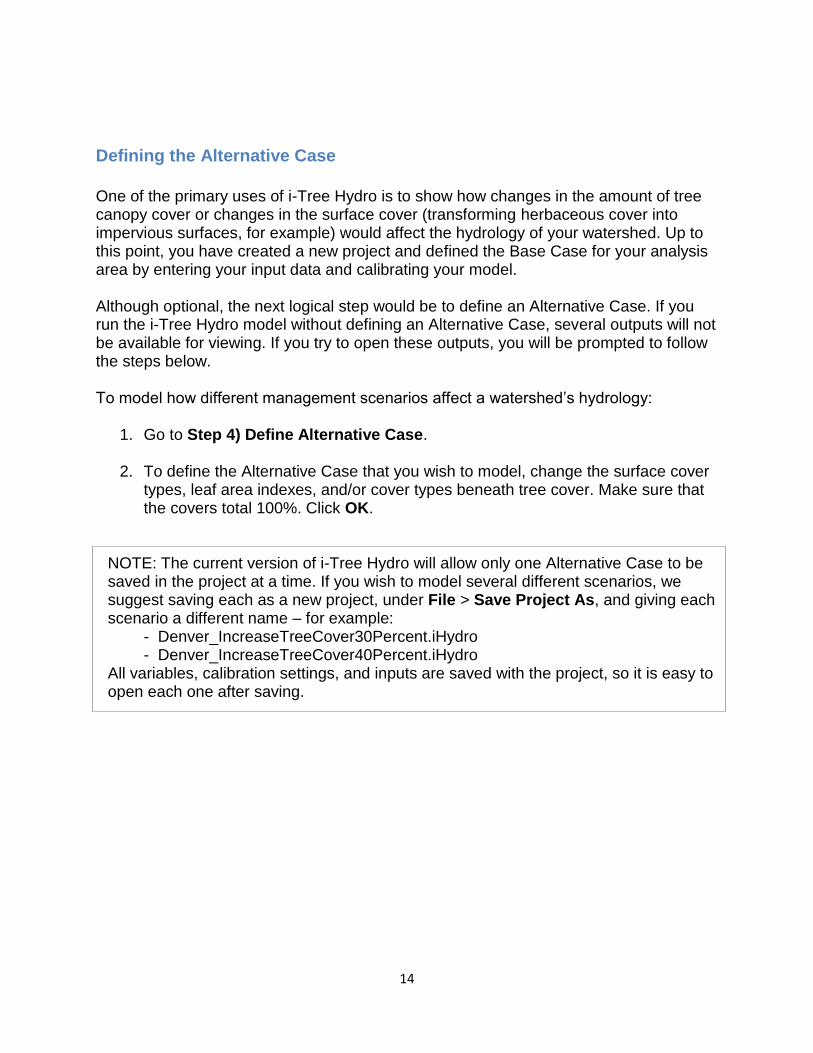
Defining the Alternative Case

One of the primary uses of i-Tree Hydro is to show how changes in the amount of tree canopy cover or changes in the surface cover (transforming herbaceous cover into impervious surfaces, for example) would affect the hydrology of your watershed. Up to this point, you have created a new project and defined the Base Case for your analysis area by entering your input data and calibrating your model. Although optional, the next logical step would be to define an Alternative Case. If you run the i-Tree Hydro model without defining an Alternative Case, several outputs will not be available for viewing. If you try to open these outputs, you will be prompted to follow the steps below. To model how different management scenarios affect a watershed’s hydrology:

1. Go to Step 4) Define Alternative Case.

2. To define the Alternative Case that you wish to model, change the surface cover types, leaf area indexes, and/or cover types beneath tree cover. Make sure that the covers total 100%. Click OK.

NOTE: The current version of i-Tree Hydro will allow only one Alternative Case to be saved in the project at a time. If you wish to model several different scenarios, we suggest saving each as a new project, under File > Save Project As, and giving each scenario a different name – for example:

- Denver_IncreaseTreeCover30Percent.iHydro - Denver_IncreaseTreeCover40Percent.iHydro

All variables, calibration settings, and inputs are saved with the project, so it is easy to open each one after saving.

15

Phase III: Exploring i-Tree Hydro Outputs i-Tree Hydro offers a variety of graphs, tables, and other model outputs that allow you to take a closer look at the hydrology and water quality modeled for your study area. Once you have run your model, you can explore these to interpret your results.

NOTE: Several outputs will not be available for viewing if you ran the Hydro model without defining an Alternative Case. If you try to open these outputs, you will be prompted to set the values in the 4) Define Alternative Case window. Refer to the last section of Phase II: Entering Model Parameters for more information.

Running the i-Tree Hydro Model

In Phases I and II, you described your project area and set up your Base Case hydrologic parameters, and possibly specified an alternative case. The final step in the process is to run the i-Tree Hydro model and view the results. Any changes to the Phase II inputs require the model to be run again in order to update the outputs. To run the i-Tree Hydro model:

1. Open Step 5) Run Hydro Model. In the window that appears, you will see the process running. It shouldn’t take more than a few minutes to run. Click OK when the top of the window reads Model run complete!

Executive Summary

One of the outputs provided by i-Tree Hydro is the Executive Summary. To open that document, go to Outputs > Executive Summary. The Executive Summary provides a broad overview of several model parameters, including the watershed area, total rainfall, total runoff, and land cover (for both the Base Case and Alternative Case, if defined). The table on the first page provides noteworthy streamflow predictions, such as highest flow, lowest flow, and average flow for the modeled Base Case and Alternative Case. There are also several graphs included in the Executive Summary:

16

1. Water Volume – compares the total volume of observed discharge of the stream gage (if supplied as an input) to the total volume of predicted streamflow of the Base Case (in cubic meters).

2. Predicted Streamflow Volume Components – displays the breakdown of the

predicted streamflow of the Base Case and Alternative Case according to the three types of streamflow the model predicts: pervious flow, impervious flow, and baseflow.

3. Pollutants: Base Case vs. Alternative Case – displays the pollutant load

(kg/month) of ten pollutants for the modeled watershed. The different pollutant loads are the predicted outputs for both the Base Case and Alternative Case.

Each output has a toolbar at the top of the window. In the Executive Summary toolbar, you will find the following tools:

1. Print – to print the output that you are viewing. When you click this tool, the Print window will appear. Select your printer name from the drop-down menu and click OK.

2. Export – to export the output that you are viewing and save it to your computer.

Next to the Export button, you will see a drop-down menu with several format options.

Outputs in a report form can be exported in PDF or RTF format. The RTF format

is compatible with Microsoft Office Word, which provides editing options.

Graphs and Tables

i-Tree Hydro produces multiple graphs and tables to display watershed hydrology. These hydrology charts can be used to contrast and compare the total volume, total flow, and streamflow components across the modeled time period. By observing the differences between the Base Case and Alternative Case, users can explore the effect of changes in land cover parameters. i-Tree Hydro can also help clarify the impacts of changes in surface cover and vegetation on pollutant load in streams by making use of a statistical parameter known as event mean concentration (EMC) (see Appendix 3: Calculating Pollution Load for more information). An EMC value represents the flow-proportional average concentration of a given pollutant during a storm event and is measured in units of mass per volume, usually milligrams per liter. EMC can be multiplied by actual flow to estimate the mass of pollutants entering a body of water, such as grams per week. Changes in flow owing to changes in cover and tree canopy will therefore be reflected in changes in pollutant load. Below are the results that i-Tree Hydro presents.

17

NOTE: EMC values can be derived from many sources, including actual measured data from your watershed. Because such actual data are hard to come by, Hydro makes use of average national values. More information about the methods used to estimate these values can be found in Appendix 3: Calculating Pollution Load. It is important to note that these are national values and therefore do not take into account local pollutant conditions and local management actions (such as street cleaning). Therefore, it is not certain how well the national EMC values will represent local conditions.

Water volume

The following Hydro outputs can be found under Outputs > Water Volume:

1. Total Streamflow – compares the total volume of observed discharge of the stream gage (supplied as an input) to the total volume of predicted streamflow of the Base Case (in cubic meters).

2. Base Case Predicted Streamflow Components – displays the breakdown of

the predicted streamflow of the Base Case according to the three types of streamflow the model predicts: pervious flow, impervious flow, and baseflow.

3. Base Case vs. Alternative Case Total Runoff – compares the total volume of

predicted discharge of the Base Case and Alternative Case, in cubic meters.

4. Base Case vs. Alternative Case Predicted Streamflow Components – compares the breakdown of the predicted streamflow of the Base Case and Alternative Case according to the three types of streamflow the model predicts: pervious flow over the land surface, impervious flow over the land surface, and baseflow through the soil media.

Each of the water volume outputs has a toolbar at the top of the window, in which you will find the following tools:

1. View – to change the view of your model output. Next to the View label, you will see a drop-down menu with options to view All, By Month, or By Week.

The View All option means that you can see the total water volume for the entire modeled time period. If you choose to view your output By Month or By Week, then the total volume will be aggregated and displayed for each month or week, respectively, of the modeled time period.

18

2. Export – to export the output that you are viewing and save it to your computer. Next to the Export button, you will see a drop-down menu with several format options.

Outputs in a graphic form can be exported as a JPG, GIF, or PNG image. Note that the exported image will be of the current view that is displayed on your screen. Graph legends are added automatically.

The water volume outputs are also customizable. Choose the colors for each bar by clicking on the colored box next to each component and then choosing your new color in the window that appears. To turn components on and off, click the check box next to the name. It may take a minute for the chart to update.

Pollution estimates

The following Hydro outputs can be found under Outputs > Pollution Estimates:

1. Base Case – displays the pollutant load (kg/unit of time) of ten pollutants for the modeled watershed. The different pollutant loads are the predicted outputs for the Base Case.

2. Base Case vs. Alternative Case – displays the pollutant load (kg/unit of time) of

ten pollutants for the modeled watershed. The different pollutant loads are the predicted outputs for both the Base Case and Alternative Case.

Each of the pollution estimate outputs has a toolbar at the top of the window, in which you will find the following tools:

1. View – to change the view of your model output. Next to the View label, you will see a drop-down menu with options to view All, By Month, or By Week.

The View All option means that you can see the total pollution load (kg) for the modeled time period. If you choose to view your output By Month or By Week, then the pollution load will be aggregated and displayed for each month or week, respectively, of the modeled time period.



Outputs in a graphic form can be exported as a JPG, GIF, or PNG image. Note that the exported image will be of the current view that is displayed on your screen. Legends are added automatically.

19

The pollution estimate outputs are also customizable. Choose the colors for each bar by clicking on the colored box next to each component and then choosing your new color in the window that appears. To turn components on and off, click the check box next to the name. It may take a minute for the chart to update.

Water flow

The following Hydro outputs can be found under Outputs > Water Flow:

1. Base Case – displays the rainfall (mm/h) and total flow (m3/h) for the modeled watershed. The rainfall values are the recorded measurements that were inputs to the model via the weather station data. The total flow is the predicted streamflow of the Base Case, including its components: baseflow, pervious flow, and impervious flow.

2. Alternative Case – displays the rainfall (mm/h) and total flow (m3/h) for the

modeled watershed. The rainfall values are the recorded measurements that were inputs to the model. The total flow is the predicted streamflow of the Alternative Case, including baseflow, pervious flow, and impervious flow.

3. Base Case vs. Alternative Case – displays the rainfall (mm/h) and compares

the total flow (m3/h) of both the Base Case and Alternative Case for the modeled watershed. The rainfall values are the recorded measurements that were inputs to the model. The total flow is displayed for the predicted streamflow of both the Base Case and Alternative Case, including baseflow, pervious flow, and impervious flow.

4. Alternative Case - Base Case – displays the rainfall (mm/h) and result of the

predicted Alternate Case flows (m3/h) minus the predicted Base Case flows (m3/h) for the modeled watershed. The rainfall values are the recorded measurements that were inputs to the model. The results of subtracting the predicted Base Case flows from the predicted Alternative Case flows are displayed to demonstrate the increase or decrease in the flows (total and component) due to changes in land cover parameters.

All of the water flow graphs show rainfall on the top of the graph, with larger rainfall events stretching towards the bottom of the graph; the rainfall rates correspond to the graph’s right-hand y-axis. Streamflow curves are on the bottom of the chart and are associated with the values on the left-hand y-axis. The x-axis represents time. Each water flow output has a toolbar at the top of the window, in which you will find the following tools:

20

1. Show All – to return the graph view to full extent. For example, if you were to zoom in on a specific segment of the graph, Show All would be used to quickly zoom back out to display the graph in its entirety.

2. Zoom In/Zoom Out – to zoom in and out on specific segments of the graph and

view the output in more detail. This is particularly useful as the full extent of the graph displays the entire modeled time period, oftentimes by month. Zooming in would allow you to view the water flow at a more specific time period, such as a day or week.

3. Pan – to move from side to side along the graph when zoomed in.




The water flow outputs are also customizable. Choose the colors for each line by clicking on the colored box next to each component and then choosing your new color in the window that appears. To turn components on and off, click the check box next to the name. It may take a minute for the chart to update. You can also view the water flow outputs in a tabular format:

1. Click on the Table tab located above the toolbar. These tables present the data numerically on an hourly basis by default.

2. There are several tools available for the tables:

a. Export – to export the output that you are viewing and save it to your

computer. Next to the Export button, you will see a drop-down menu with several format options.

Outputs in a tabular form can be exported in Excel or comma-separated values (CSV). Both of these file types are compatible with Microsoft Office Excel, which provides relatively easy editing.

b. Total by – to change the view of your model output. In the Total by drop-

down menu, you can choose to display daily totals, weekly totals, monthly totals, or a total for the entire model run period (usually, but not always, one year).

21

Water pollution

The following Hydro outputs can be found under Outputs > Water Pollution:

1. Base Case – displays the rainfall (mm/h) and pollutant load (kg/h) of ten pollutants for the modeled watershed. The different pollutant loads are the predicted outputs for the Base Case.

2. Alternative Case – displays the rainfall (mm/h) and pollutant load (kg/h) of ten

pollutants for the modeled watershed. The different pollutant loads are the predicted outputs for the Alternative Case.

3. Alternative Case - Base Case – displays the rainfall (mm/h) and change in

pollutant load (kg/h) between the Base Case and Alternate Case for the modeled watershed. The rainfall values are the recorded measurements that were inputs to the model. The pollutants loads are the predicted model outputs for the Base Case and Alternative Case. Displaying the pollutant loads against the rainfall allows the user to observe how the pollutant load changes during and after a precipitation event. This graph enables a user to compare the pollutant loads of the current Base Case against the pollutant loads of an Alternative Case. Such a comparison allows for observation of the effects (positive or negative) on the pollutant load present in the total flow (discharge) associated with the proposed changes to tree cover, land cover, etc.

All of the water pollution graphs show rainfall on the top of the graph, with larger rainfall events stretching towards the bottom of the graph; the rainfall rates correspond to the graph’s right-hand y-axis. Pollutant load measurements are on the bottom of the chart and are associated with the values on the left-hand y-axis. The x-axis represents time. Each water pollution output has a toolbar at the top of the window, in which you will find the following tools:



view the output in more detail. This is particularly useful as the full extent of the graph displays the entire modeled time period, oftentimes by month. Zooming in would allow you to view the pollutant load at a more specific time period, such as a day or week.

3. Pan – to move from side to side along the graph when zoomed in.

22

4. Export – to export the output that you are viewing and save it to your computer. Next to the Export button, you will see a drop-down menu with several format options.


The water pollution outputs are also customizable. Choose the colors for each line by clicking on the colored box next to each component and then choosing your new color in the window that appears. To turn components on and off, click the check box next to the name. It may take a minute for the chart to update. To view the water pollution outputs in a tabular format:

1. Click on the Table tab located above the toolbar. These tables present the data numerically on an hourly basis by default.

2. There are several tools available for the tables:

a. Export – to export the output that you are viewing and save it to your


Outputs in a tabular form can be exported in Excel or comma-separated values (CSV). Both of these file types are compatible with Microsoft Office Excel, which provides relatively easy editing.

b. Total by – to change the view of your model output. In the Total by drop-

down menu, you can choose to display daily totals, weekly totals, monthly totals, or a total for the entire model run period (usually, but not always, one year).

DEM 2D/3D Visualization

If your elevation input was a DEM file, you can view two-dimensional and three-dimensional representations of your Digital Elevation Model (DEM) by navigating to Outputs > DEM 2D/3D Visualization. Given the Universal Transverse Mercator (UTM) projection of the DEM data, the watershed may appear distorted. This option is not available for projects using a Topographic Index (TI) instead of a DEM. When viewing the 3D simulation, press and hold the cursor in the viewing window while moving the cursor to change the view of your DEM.

23

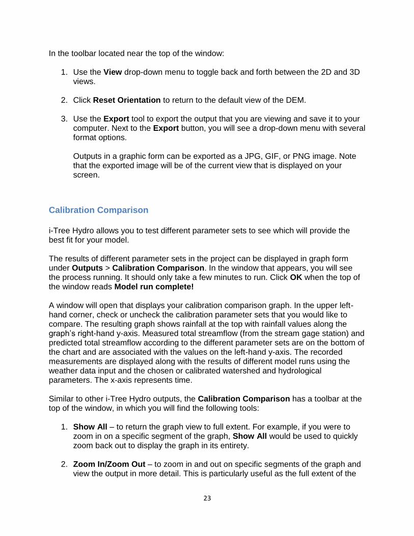
In the toolbar located near the top of the window:

1. Use the View drop-down menu to toggle back and forth between the 2D and 3D views.

2. Click Reset Orientation to return to the default view of the DEM.

3. Use the Export tool to export the output that you are viewing and save it to your


Outputs in a graphic form can be exported as a JPG, GIF, or PNG image. Note that the exported image will be of the current view that is displayed on your screen.

Calibration Comparison

i-Tree Hydro allows you to test different parameter sets to see which will provide the best fit for your model. The results of different parameter sets in the project can be displayed in graph form under Outputs > Calibration Comparison. In the window that appears, you will see the process running. It should only take a few minutes to run. Click OK when the top of the window reads Model run complete! A window will open that displays your calibration comparison graph. In the upper left-hand corner, check or uncheck the calibration parameter sets that you would like to compare. The resulting graph shows rainfall at the top with rainfall values along the graph’s right-hand y-axis. Measured total streamflow (from the stream gage station) and predicted total streamflow according to the different parameter sets are on the bottom of the chart and are associated with the values on the left-hand y-axis. The recorded measurements are displayed along with the results of different model runs using the weather data input and the chosen or calibrated watershed and hydrological parameters. The x-axis represents time. Similar to other i-Tree Hydro outputs, the Calibration Comparison has a toolbar at the top of the window, in which you will find the following tools:



view the output in more detail. This is particularly useful as the full extent of the

24

graph displays the entire modeled time period, oftentimes by month. Zooming in would allow you to view the pollutant load at a more specific time period, such as a day or week.

3. Pan – to move from side to side along the graph when the zoomed in.




Extended Outputs for Advanced Users

In order to share results from model sub-routines (including interception, infiltration,

evaporation & evapotranspiration), the Hydro model generates extended outputs in a

project’s working directory as it completes simulations. This has been done by

implementing a method used in the past by i-Tree Hydro researchers & developers in

testing the model. In i-Tree Hydro version 5.1, extended outputs are not included in the

Graphical User Interface (GUI) yet, and accessing these results is slightly more

technical.

To view extended outputs of a specific Hydro run, you’ll need to identify and navigate to

your Working Directory. The easiest way to do this is by setting one specifically for your

project. While configuring that, you can also confirm that the option Run with Extended

Outputs is enabled.

Enabling extended outputs & configuring your working directory

Go to Help > Options, enable the options Run with Extended Outputs and Use

Specified Working Directory for Hydro Model Processing by checking off their respective

boxes, and then set your Working Directory by clicking Browse as shown in Figure 2.

25

Fig. 2: Screenshot of Options window, enabling Extended Outputs & setting Working

Directory for project

Accessing & understanding extended outputs of a specific Hydro run

After you’ve run the simulations you are interested in extended outputs for, navigate to

the Working Directory for that simulation of interest. There you’ll find files which include

outputs extended beyond what’s included in the i-Tree Hydro GUI.

The following is a list highlighting and explaining some extended outputs of interest:

output.dat – A summary of key outputs, many of which are reported within i-Tree

Hydro. Time-series in this file can be accessed through the i-Tree Hydro GUI in

more user-friendly formats (including as CSV files).

VegCanopyFile.csv – Features of the water balance for vegetation processes.

WaterOnPerArea.csv – Features of the water balance for pervious area

processes.

WaterOnImpArea.csv – Features of the water balance for impervious area

processes.

Evap_ET_Infil.csv – Outputs related to evaporation from vegetation surfaces,

infiltration, and evapotranspiration from the root zone.

26

Each of these extended output .csv files comes in two versions marked with either a

_VW or _FW suffix. The ‘VW’ versions represent the one-dimensional Vertical Water

Balance or Flux results, with outputs computed as depths to be statistically-distributed

throughout the project area. The ‘FW’ versions represent the statistically-distributed

‘Final Water’ Balance or Flux results, with VWB depths being multiplied by applicable

land cover percentages and the project area to produce volumetric results.

Acronyms and phrases used in column titles identify data within each of the extended

output files. The following lists provide definitions to clarify these files:

General Definitions

W - water WB - water balance WF - water flux SWE - snow water equivalent SWEB - snow water equivalent balance Comb - combined water balance from water and snow water equivalent OIA - open impervious area TCIA - tree cover over impervious area TCPA - tree cover over pervious area TC - total tree cover (over both pervious + impervious) IA - total impervious cover (open impervious area + impervious area under tree cover) SV - short vegetation cover BS - bare soil cover nonRouted - runoff has not been distributed in time using the 2 parameter surface routing equation

VegCanopyFile Column Definitions

Rain - total rain falling onto the project area SWE - total snow water equivalent falling onto the project area Rain_TC - rain falling on the tree canopy SWE_TC - snow water equivalent falling on the tree canopy Intercept_TC_W - rain intercepted by the tree canopy Intercept_TC_SWE - snow water equivalent intercepted by the tree canopy Evap_TC_W - evaporation of water from tree canopy leaf storage Evap_TC_SWE - evaporation of snow water equivalent from tree canopy leaf storage LeafStore_TC_W - water stored in tree canopy leaf storage LeafStore_TC_SWE - snow water equivalent stored in tree canopy leaf storage ThroughFall_TC_W - water throughfall through the tree canopy ThroughFall_TC_SWE - snow water equivalent throughfall through the tree canopy TreeCanopy_WB - tree canopy water balance (SWE and W combined) Rain_SV - rain falling on the short veg canopy SWE_SV - snow water equivalent falling on the short veg canopy Intercept_SV_W - rain intercepted by the short veg canopy Intercept_SW_SWE - snow water equivalent intercepted by the short veg canopy Evap_SV_W - evaporation of water from short veg canopy leaf storage Evap_SV_SWE - evaporation of snow water equivalent from short veg canopy leaf storage LeafStore_SV_W - water stored in short veg canopy leaf storage LeafStore_SV_SWE - snow water equivalent stored in short veg canopy leaf storage ThroughFall_SV_W - water throughfall through the short veg canopy ThroughFall_SV_SWE - snow water equivalent throughfall through the short veg canopy ShortVegCanopy_WB - short veg canopy water balance (SWE and W combined)

WaterOnPerArea Column Definitions

Rain - total rain falling onto the project area

27

Rain_BS - rain falling onto the bare soil area ThroughFlow_TCPA_W - throughflow of water onto the pervious area under tree cover ThroughFlow_SV_W - throughflow of water onto the pervious area under short veg cover SnowMelt_TCPA - snow melt on the pervious area under tree cover SnowMelt_SV - snow melt on the pervious area under short veg cover SnowMelt_BS - snow melt on the pervious area bare soil Water_PA - total water on the total pervious area PerArea_WB - water balance for the water on pervious area routines SWE - total snow water equivalent falling onto the project area SWE_BareSoil - total snow water equivalent falling onto the bare soil area ThroughFlow_TCPA_SWE - throughflow of snow water equivalent onto the pervious area under tree cover ThroughFlow_SV_SWE - throughflow of snow water equivalent onto the pervious area undershort veg cover SWE_on_TCPA - snow water equivalent on the pervious area under tree cover SWE_on_SV - snow water equivalent on the pervious area under short veg cover SWE_on_BS - snow water equivalent on the bare soil area SnowSub_TCPA - sublimation of snow water equivalent on the pervious area under tree cover SnowSub_SV - sublimation of snow water equivalent on the pervious area under short veg cover SnowSub_BS - sublimation of snow water equivalent on the bare soil area PerArea_SWEB - snow water equivalent balance for the SWE on pervious area routines PerArea_comb_WB - combined (summed) water balance for W and SWE on the pervious area routines Water_PA - total water on the total pervious area Run_on_from_IA - overflow from the depression storage of the total impervious area to pervious areas Inflow_to_PerDep - total flow into pervious depression storage (summed run-on from IA + total water on PA) PerDepStor_PA - depression storage of the total pervious area PerDepEvap_PA - evaporation from depression storage of the total pervious area PerFlow_To_Infil - overflow from the depression storage of the total pervious area to the infiltration routine PA_Flow_To_Infil_WB - water balance for the pervious area flow to infiltration routines

WaterOnImpArea Colum Definitions

Rain_OIA - rain on the open impervious area ThroughFlow_TCIA_W - throughflow of water onto the impervious area under tree cover SnowMelt_OIA - snow melt on the open impervious area SnowMelt_TCIA - snow melt on the impervious area under tree cover Water_IA - total water on the total impervious area ImpArea_WB - water balance for the water on impervious area routines SWE_OIA - snow water equivalent on the open impervious area ThroughFlow_TCIA_SWE - throughflow of snow water equivalent onto the impervious area under tree cover SWE_on_OIA - snow water equivalent on the open impervious area SWE_on_TCIA - snow water equivalent on the impervious area under tree cover SnowSub_OIA - sublimation of snow water equivalent on the open impervious area SnowSub_TCIA - sublimation of snow water equivalent on the impervious area under tree cover ImpArea_SWEB - snow water equivalent balance for the SWE on impervious area routines ImpArea_comb_WB - combined (summed) water balance for W and SWE on the impervious area routines ImpDepStor_IA - depression storage of the total impervious area ImpDepEvap_IA - evaporation from the depression storage of the total impervious area ImperFlow_Soil - overflow from the depression storage of the total impervious area to pervious areas ImperFlow_Outlet_nonRouted - overflow from the depression storage of the total impervious area to the runoff routing routine ImpArea_Runoff_WB - water balance for the impervious area runoff generation routines

Evap_ET Column Definitions

Evap_TC_W - evaporation of water from tree canopy leaf storage Evap_TC_SWE - evaporation of snow water equivalent from tree canopy leaf storage Evap_SV_W - evaporation of water from short veg canopy leaf storage Evap_SV_SWE - evaporation of snow water equivalent from short veg canopy leaf storage Infiltration_PA - water infiltrated by the pervious area rET_VegCover - real (not potential) evapotranspiration

28

Additional Information

Choosing Your Watershed and Gaging Station

If you pursue a watershed analysis instead of the non-watershed option, then the first, and perhaps most difficult, decision you have to make is selecting a watershed to analyze. One challenge here is that many people are more accustomed to thinking in terms of political or parcel boundaries (e.g. a city or a university campus) and considering what impacts might result from changes within those areas. Hydrological modeling often occurs at the watershed level, which tends not to align with political or parcel boundaries. A second challenge relates to the availability of data. i-Tree Hydro makes use of hourly stream gage data from the U.S. Geological Survey (USGS). Although there are many stream gage stations across the country, data are not available for every stream and its associated watershed. A third challenge relates to scale. Gages are located in streams that capture water from watersheds of vastly different scales. A stream gage in a small creek might be associated with a watershed of a few square kilometers. A stream gage at the mouth of the Mississippi River would be associated with a watershed that includes half of the United States. Because of the effect of scale, care needs to be taken to make sure project area and land cover percentages appropriately represent the intended scenario. With these limitations in mind, your goal in this first step is to choose the best stream gage station in your area of interest and estimate the boundaries of the associated watershed. You’ll use these boundaries in conjunction with obtaining your digital elevation model data and land cover data.

Tools for choosing the best stream gage station and watershed:

The easiest method for visualizing stream gage stations and their associated watersheds is Google Earth. Begin by downloading the two files necessary:

1. At the EPA’s Waters website (https://www.epa.gov/waterdata/viewing-waters-data-using-google-earth), download the WATERS Data 1.5(Vector).kmz file (or the most current version posted).

NOTE: Links were correct at time of publication but may have changed. If necessary, please use the EPA website’s search box and relevant key words (“WATERS, Google Earth, KMZ”) to search for updated links.

2. From www.itreetools.org > Resources > Archives under the Hydro section,

https://www.epa.gov/waterdata/viewing-waters-data-using-google-earth

https://www.epa.gov/waterdata/viewing-waters-data-using-google-earth


29

download the zip file of the stream gage stations available in Hydro: i-Tree_Hydro_Gaging Stations_2005.

3. Open Google Earth on your computer (version 5.0 or higher) and open the two

files. Zoom in to your area of interest (see Figure 3).

A few hints: (1) The EPA Waters file is live – that is, it updates from the internet while you are using it. Therefore it can be very slow. You’ll know it is gathering data when the little colored boxes next to the field names under Places are spinning. To speed things up, uncheck every box under Surfacewater Features, except Streams, and all boxes associated with Water Program Features, and zoom in to your area. (2) The streams are only visible at very local scales. If you can’t see them, continue zooming in until the scale at the bottom of the map is approximately 1 inch = 3 miles. Remember to wait for the data to load.

Fig. 3: Streams and stream gage stations around Denver

4. The next step is to explore the watersheds associated with each station to

choose the best one. To do this:

a. Click on the stream itself just downstream of the station. A window will appear describing the features of the stream. At the bottom, under Tools, click Drainage Area Delineation.

b. In the window that appears, choose Stop When: Maximum Distance

(KM) = 30 and click Start Search. The watershed upstream from that

30

point for the first 30 km will be identified. You might have to repeat this process a few times, increasing the maximum distance to capture the entire watershed (see Figure 4).

Fig. 4: A watershed near Denver

Fig. 5: A smaller watershed near Denver

31

NOTE: To check that you are examining the entire watershed associated with a stream gauge, you can check the drainage basin area on the USGS Water Resources website summary page for the stream gauge. To do so, enter your 8-digit stream gauge ID into the following URL replacing the bold X’s, and then navigate to that updated URL in a web browser: http://waterdata.usgs.gov/nwis/inventory/?site_no=XXXXXXXX&agency_cd=USGS

Example: For gauge 01648000, navigate to… http://waterdata.usgs.gov/nwis/inventory/?site_no=01648000&agency_cd=USGS In the Description for the Stream Site, you can find Drainage Area in square miles.

Example: For gauge 0164800, the drainage area is 62.2 square miles.

c. Once you have determined the outline of the watershed, judge whether it is appropriate for your study.

Does it capture your area of interest? Is the watershed of a scale that would be appropriate for modeling changes in canopy and impervious cover? (As explained above, if the watershed is very large, changes in cover are unlikely to have a measurable impact.)

d. Delineate the drainage areas for other stream gage stations until you have

found the best one (see Figure 5).

5. Once you have made your selection:

a. Note the name of the stream by clicking on the stream.

b. Note the ID number of the stream gage station (SITENO), by clicking on its red dot.

c. Capture an image of the stream gage station and watershed using your

computer’s Print Screen function or Google Earth’s File > Save > Save Image function.

Gathering Data

Now that you have selected your watershed of interest and the appropriate stream gage, it is time to start gathering your input data. In Phase I: Creating a New Project, we described the general input data that is needed for a new project in i-Tree Hydro. The following tables and directions will assist you in collecting the data that you will need in order to run i-Tree Hydro, including some possible data sources or suggested default values.

http://waterdata.usgs.gov/nwis/inventory/?site_no=01648000&agency_cd=USGS

32

Basic watershed characteristics

The following input data can be entered by going to Step 1) Project Area Information:

Table 1. Basic Watershed Characteristics

Category Sourcea

Default value Units

Watershed Land Area DEM, TI N/A km2

or mi2

Percent Tree Cover Eco, Canopy,

N/A % UTC, GIS

Tree Leaf Area Indexb Eco, Canopy,

4.7 none

UTC, GIS

Evergreen Tree Cover Eco, GIS 10 %

Evergreen Shrub Cover Eco, GIS 10 %

State Date/Time (Local) N/A N/A mm/dd/yyyy

hh:mm:ss

End Date/Time (Local) N/A N/A mm/dd/yyyy

hh:mm:ss a DEM = Digital Elevation Model data (see ). TI = Topographic Index data (see Appendix 2: Topographic Index Data). Eco = An existing i-Tree Eco study; although it is unlikely that the Eco study area and the Hydro study area will align exactly, your Eco results may still have relevant and useful information. Canopy = i-Tree Canopy. Visit www.itreetools.org for more information on i-Tree Eco and i-Tree Canopy. UTC = An existing urban tree canopy analysis. GIS = Your local government or university GIS department. b Leaf area indexes (LAI) can be calculated from Eco results for leaf area, which are presented in units of m2/ha. Divide those results by 10,000, to get LAI.

Digital Elevation Model (DEM)

Once you have identified your project area, your next step is to create a Digital Elevation Model (DEM) of the watershed. The end product should be a DEM clipped to the boundaries of the area, projected in the proper Universal Transverse Mercator (UTM) coordinate zone in meters, and converted to ASCII computer code format. For more specifics on this process, see Appendix 1.

Topographic Index (TI)

Topographic Index (TI) data are derived from DEM data within various polygon boundaries. If you opt to use a pre-loaded Topographic Index (TI), you can skip creating a DEM for your project area. i-Tree Hydro contains a TI histogram database based on USGS calculations, with tables for States, Counties, Places, gaged Watershed Basins,

33

and HUC8 watersheds. In each table there is a minimum and maximum topographic index value and a count of the number of pixels in the area of interest. The B1 - B30 fields contain the proportion of the pixels in the area of interest that fall within that histogram bin. For a brief overview on how the TIs were constructed, see Appendix 2: Topographic Index Data.

Observed streamflow

Streamflow data are used in i-Tree Hydro to calibrate the model. Hydro tries to find the best fit between the streamflow predicted by the model and the streamflow measured at the stream gage station. However, stream gage availability varies and not every stream has a gage located on it. Within i-Tree Hydro, hourly streamflow data are available as standardized, complete data sets. These data were obtained from the U.S. Geological Survey and pre-processed for 2005-2012. If you choose to use the available data, follow the steps provided in Phase I: Creating a New Project to choose your gage from a map. If you are interested in using data from a different year or you would like to use data for a gage that is not included in Hydro, then you have the option of using your own streamflow data. Once you have obtained your streamflow data, it is very important that the data are properly formatted for use in i-Tree Hydro. Raw observed streamflow data must consist of the following fields: Table 2. Raw Observed Streamflow Data Fields

Field namea Definition

b

Units

site_no site identification number N/A

date_time

date and time of observation

YYYYMMDDhhmmss

tz_cd time zone N/A

dd

data descriptor

N/A

accuracy_cd accuracy code N/A

value

discharge

cfs

precision digits of precision in the discharge N/A

remark

optional remark code

N/A

a Required fields include: date_time, tz_cd, and value. See note below. b For a list of accuracy codes and optional remark codes, see the example stream data at Resources> Archives > i-Tree Hydro Resources at www.itreetools.org.


34

To make your data compatible with Hydro, the fields should be organized in tab-separated columns using the field names listed above and saved as an .rdb file. When streamflow data are properly formatted, you will be able to navigate to the folder in which you saved it and load it into the 1) Project Area Information form as described in Phase I: Creating a New Project.

NOTE: Not all of the fields listed are used in i-Tree Hydro. If you cannot find certain information, the field name still needs to be included, but you can populate the column with dummy values. For example, i-Tree Hydro does not use the accuracy code, but due to formatting of the data, a placeholder value is needed to keep the application on track.

An example of correctly formatted streamflow data can be found at www.itreetools.org > Resources > Archives > i-Tree Hydro Resources.

Weather station

Weather station data are an important input because they are used to simulate the streamflow of your study area. When selecting your weather station be sure to select a station that is representative of your entire study area. Bear in mind that precipitation events may be highly localized, so there may be times when it is raining in the watershed but not at the weather station or vice versa. This can make it challenging for auto-calibration to match observed and predicted streamflow. For that reason, it can be difficult to choose the best weather station and may mean that you have to try several different options. Within i-Tree Hydro, hourly weather and evapotranspiration data are available as standardized, complete data sets. These data are obtained from the National Oceanic and Atmospheric Administration’s (NOAA) National Climatic Data Center (NCDC) and pre-processed for 2005-2012. If you choose to use the available data, then follow the steps provided in Phase I: Creating a New Project to choose your station from a map. If you are interested in using data from a different year or you would like to use data from a weather station that is not included in Hydro, then you have the option of using your own weather station data. Required weather data include wind direction and speed, cloud ceiling, sky cover, temperature, dewpoint, altimeter setting, pressure, and hourly precipitation. Once you have obtained your weather station data, it is very important that the data are properly formatted for use in i-Tree Hydro. Weather station data must consist of the following fields:


35

Table 3. Weather Station Data Fields

Field name Definitionb

Units

USAF Air Force catalog station number N/A

WBAN

NCDC WBAN number

N/A

YR--MODAHRMN year-month-day-hour-minute in GMT YYYYMMDDhhmm

DIRa

wind direction in compass degrees

N/A

SPDa wind speed mph

GUS

wind gust

mph

CLGa

cloud ceiling – lowest opaque layer with

5/8 or greater coverage

hundreds of ft

sky cover (clr-clear, sct-scattered [1/8 -

SKCa 4/8], bkn-broken [5/8 - 7/8], ovc-overcast, N/A

obs -obs cured, pob-partial obs curation)

L low cloud type N/A

M middle cloud type N/A

H

high cloud type

N/A

VSB visibility in statute mi (nearest tenth)

WW WW WW present weather N/A

W

past weather indicator N/A

TEMPa temperature °F

DEWPa

dewpoint

°F

SLP sea level pressure mbar (nearest tenth)

ALTa

altimeter setting

in (nearest hundredth)

STPa station pressure mbar (nearest tenth)

MAX maximum temperature °F

MIN minimum temperature °F

PCP01a 1-hour liquid precipitation in (nearest hundredth)

PCP06

6-hour liquid precipitation

in (nearest hundredth) PCP24 24-hour liquid precipitation in (nearest hundredth)

PCPXX liquid precipitation for a period other 1, 6, or 24 hours

in (nearest hundredth)

SD snow depth in a Required fields include: DIR, SPD, CLG, SKC, TEMP, DEWP, ALT or STP, PCP01. See note below. b For weather code tables, go to Resources > Archives > i-Tree Hydro Resources > i-Tree Hydro weather abbreviation codes at www.itreetools.org.


36

To make your data compatible with Hydro, the fields should be organized in tab-separated columns using the field names listed above and saved as an .rdb file. When weather station data are properly formatted, you will be able to navigate to the folder in which you saved it and load it into the 1) Project Area Information form as described in Phase I.

NOTE: Not all of the fields listed are used in i-Tree Hydro. If you cannot find that information, the field name still needs to be included, but you can populate the column with dummy values. For example, i-Tree Hydro does not use the altimeter setting, but due to formatting of the data, a placeholder value is needed to keep the application on track.

An example of correctly formatted raw weather station data can be found at www.itreetools.org > Resources > Archives > i-Tree Hydro Resources.

Land cover parameters

The following input data can be entered by going to Step > 2) Land Cover Parameters: Table 4. Land Cover Parameters

Category Sourcea

Default value Units

Tree Coverb

Eco, Canopy,

UTC, GIS

Shrub Coverb

Eco, Canopy,

UTC, GIS

Herbaceous Coverb Eco, Canopy,

UTC, GIS

Water Coverb

Eco, Canopy,

UTC, GIS

Impervious Coverb Eco, Canopy,

UTC, GIS

Soil Coverb

Eco, Canopy, N/A %

UTC, GIS

Tree Leaf Area Indexc

Eco, Literature 4.7 none

Shrub Leaf Area Indexc


Herbaceous Leaf Are Indexc


Directly Connected Impervious Aread

GIS 40 %

Cover Types Beneath Trees (Should total 100%)

Pervious Cover

Eco, Canopy

N/A

%

N/A %

N/A %

N/A % N/A % N/A %


37

Impervious Cover Eco 6.1 %

a DEM = Digital Elevation Model data (see ). Eco = An existing i-Tree Eco study; although it is unlikely that the Eco study area and the Hydro study area will align exactly, your Eco results might offer some insight. Canopy = i-Tree Canopy. Visit www.itreetools.org for more information on i-Tree Eco and i-Tree Canopy. UTC = an existing urban tree canopy analysis. GIS = your local government or university GIS department. Literature = some data may be available for certain locations in the scientific literature or from the appropriate university department. b Surface Cover Types (should total 100%) c Leaf area indexes (LAI) can be calculated from Eco results for leaf area. d DCIA can be particularly difficult to find. One strategy is to adjust the value in the calibration process until the model streamflow resembles the observed streamflow; see Calibrating the Model to learn more.

Leaf Area Index (LAI)

Leaf Area Index (LAI) is the total leaf area divided by the canopy area. More specifically, it is the ratio of 1-sided surface area of leaves (m) per unit canopy cover (m). LAI is a dimensionless variable describing leaf area density per canopy cover. A way to think about LAI is to imagine drawing a square on the ground under a tree canopy, with sides 1 meter in length. Standing in this 1-meter square area, looking up into the tree canopy, the LAI represents the surface area (1-sided) of the leaves present directly above this 1 meter square area. Typical LAI values range from 1-7, representing 1-7 square meters of leaf area (1-sided) above this 1-meter square area. Leaf area index can be derived from certain i-Tree Eco results. When deriving leaf area index for i-Tree Hydro, it is important keep in mind that leaf area index is the leaf area per unit canopy cover. Some variables in i-Tree Eco describe the density of leaves in a certain strata or land use, or per unit ground cover within the entire project area. The difference is due to what each tool is designed for: in Eco, the interest in leaf area is describing tree canopy in the context of a city, a strata, a land use, etc.; in Hydro, the interest is the properties of tree canopy itself wherever it exists in the project area.

Directly Connected Impervious Area (DCIA)

DCIA is the portion of impervious cover that drains directly to the modeled stream or any of its tributaries. The phrase “drains directly” describes a situation where precipitation that falls on a portion of the watersheds impervious cover is conveyed, overland or through a storm sewer network, directly into the stream or its tributaries. For example, rain that falls on a parking lot could travel over the asphalt surface to a storm sewer inlet, where the precipitation then travels through the storm sewer network to an outfall which discharges into the stream. The parking lot in this example would be considered a directly connected impervious area. DCIA does not include: impervious area (IA) draining to stormwater practices designed to meet recharge and other volume reduction criteria; isolated IA with an indirect hydraulic connection to the MS4, or that otherwise drain to a pervious area; swimming

38

pools or man-made impoundments, unless drained to an MS4; the surface area of natural waterbodies (e.g., wetlands, ponds, lakes, streams, rivers). DCIA is initially calculated based on impervious cover estimates according to the equations put forth by Sutherland (2000) and recommended by the EPA in its Small MS4 Permit Technical Support Document (2011). See Tables 5 and 6 for guides for estimating impervious area and the Sutherland equations. Table 5. Estimate of Percent Impervious Area as a Function of Land Use (Reproduced from USEPA 2011b.)

Land Use % IA

Commercial 76

Industrial 56

High Density residential 51

Medium density residential 38

Low Density Residential 19

Institiutional 34

Agricultural 2

Forest 1.9

Open Urban Land 11

Table 6. Sutherland Equations to Determine DCIA (%) (Reproduced from USEPA 2011a.)

Watershed Selection Criteria

Assumed Land Use Equation

(where IA (%) ≥ 1)

Average: Mostly storm sewered with curb & gutter, no dry wells or infiltration, residential rooftops not directly connected

Commercial, Industrial, Instititutional, Open land, and Medium density residential

𝐷𝐶𝐼𝐴 = 0.1(𝐼𝐴)1.5

Highly concentrated: Same as above, but residential rooftops are connected

High density residential 𝐷𝐶𝐼𝐴 = 0.4(𝐼𝐴)1.2

Totally connected: 100% storm sewered with all IA connected

-- 𝐷𝐶𝐼𝐴 = 𝐼𝐴

Somewhat connected: 50% not storm sewered, but open section roads, grassy swales, residential rooftops not connected, some infiltration.

Low density residential 𝐷𝐶𝐼𝐴 = 0.04(𝐼𝐴)1.7

Mostly disconnected: Small percentage of urban area is storm sewered, or 70% or more infiltrate/disconnected

Agricultural, Forested 𝐷𝐶𝐼𝐴 = 0.01(𝐼𝐴)2

39

After you have estimated the percent impervious area and DCIA for your watershed base case, you need to determine how changing land use will change your DCIA. A simple scenario will involve recalculating the percent of impervious area and then recalculating DCIA. However, methods have been developed that can show the influence of adding green infrastructure to your watershed more precisely than simply determining how much IA was replaced with plant cover. To determine how much IA and DCIA have been added or removed as a result of individual development, redevelopment, or retrofit projects, you need to know the effectiveness of stormwater best management practices (BMPs) you are adding to your watershed to reduce associated runoff and how much runoff from impervious areas they are treating. BMPs that reduce runoff volume lower DCIA, while practices that remove stormwater pollutants but do not provide runoff reduction benefits are not effective at reducing DCIA. For each BMP you are simulating in your model, there is a “disconnection” multiplier (Table 7 and Equation 1) to determine how much your BMP is reducing the DCIA. Infiltration trenches and basins reduce DCIA based on soil infiltration rates and the runoff depth captured; the volume of runoff reduction is shown in Table 8 and was derived from the EPA 2010 BMP Performance Curves. If your simulation involves adding new IA (i.e. you are building a new parking lot with a detention basin and would like to determine its impact on the watershed) then use Equation 2 to determine the amount of DCIA you are adding to the watershed. If your simulation isn’t adding any IA to your watershed and is just adding BMPs (i.e. you are replacing an existing parking lot with permeable pavement) then use Equation 3 to determine the amount of DCIA your project is reducing.

𝐷𝑖𝑠𝑐𝑜𝑛𝑛𝑒𝑐𝑡𝑖𝑜𝑛 𝑀𝑢𝑙𝑡𝑖𝑝𝑙𝑖𝑒𝑟 =1 − % 𝑅𝑢𝑛𝑜𝑓𝑓 𝑅𝑒𝑑𝑢𝑐𝑡𝑖𝑜𝑛 𝑉𝑜𝑙𝑢𝑚𝑒

100 (𝐄𝐪𝐧. 𝟏)

𝐴𝑑𝑑𝑒𝑑 𝐷𝐶𝐼𝐴𝐵𝑀𝑃𝑖 = 𝐼𝐴𝐵𝑀𝑃𝑖 × 𝐷𝑖𝑠𝑐𝑜𝑛𝑛𝑒𝑐𝑡𝑖𝑜𝑛 𝑀𝑢𝑙𝑡𝑖𝑝𝑙𝑖𝑒𝑟 (𝐄𝐪𝐧. 𝟐) 𝑅𝑒𝑑𝑢𝑐𝑒𝑑 𝐷𝐶𝐼𝐴𝐵𝑀𝑃𝑖 = 𝐼𝐴𝐵𝑀𝑃𝑖 × (1 − 𝐷𝑖𝑠𝑐𝑜𝑛𝑛𝑒𝑐𝑡𝑖𝑜𝑛 𝑀𝑢𝑙𝑡𝑖𝑝𝑙𝑖𝑒𝑟) (𝐄𝐪𝐧. 𝟑)

Calculate the added or reduced DCIA for every BMP you wish to simulate, then sum the added DCIAs and subtract the reduced DCIAs to determine the overall change in DCIA for your watershed. If you simulated the addition of IA, adjust that parameter too. Table 7. Determining DCIA based on Interim Default BMP Disconnection Multipliers or EPA’s Infiltration Curves (from USEPA 2011a)

BMP Description % Runoff Volume Reduction1

BMP Disconnection

Multiplier2

Removal of pavement; restoration of infiltration capacity

100% 0

Redirection of rooftop runoff to infiltration areas, rain gardens or

85% 0.15

40

dry wells

Permeable pavement, bioretention practices, dry/vegetated water quality swales

75% 0.25

Disconnection to qualified pervious area3

50% 0.50

Infiltration trenches 15-100% 0.85-0

Infiltration basins 13-100% 0.87-0

Non-runoff reduction practices (i.e., detention ponds, wetlands, sand filters, hydrodynamic separators, etc)

0% 1.0

1 Interim default values for % runoff reduction are based on Schueler, 2009 and are subject to change as more data becomes available. Values for infiltration trenches and basins are based on soil infiltration rates and depth of runoff treated. See Tables 8 to determine the site specific values to apply. 2 BMP multiplier = 1 - % Runoff Volume Reduction / 100 3 Areas given MassDEP LID Site Design Credits per the MA Stormwater Standards (Vol. 3, Chapter 1) are assigned % reduction values based on upper estimates of rooftop disconnection to pervious area as reported by Chesapeake Stormwater Network, 2009.

Table 8. Percent Runoff Reduction based on EPA’s 2010 Infiltration Curves (from USEPA 2011a)

Depth of Runoff Treated (inches)

Soil Infiltration Rate (in/hr)

0.17 0.27 0.52 1.02 2.41 8.27

Infiltration Trench

0.1 15% 18% 22% 26% 34% 54%

0.2 28% 32% 38% 45% 55% 76%

0.4 49% 55% 62% 68% 78% 93%

0.6 64% 70% 76% 81% 88% 97%

0.8 75% 79% 84% 88% 93% 99%

1.0 82% 85% 89% 92% 96% 100%

1.5 92% 93% 95% 97% 99% 100%

2.0 95% 96% 97% 98% 100% 100%

Infiltration Basin

0.1 13% 16% 20% 24% 33% 55%

0.2 25% 30% 36% 42% 54% 77%

0.4 44% 51% 58% 66% 78% 93%

0.6 59% 66% 73% 79% 88% 98%

0.8 71% 76% 81% 87% 93% 99%

1.0 78% 82% 87% 91% 96% 100%

1.5 89% 91% 94% 96% 99% 100%

2.0 94% 95% 97% 98% 100% 100%

41

Calibrating the Model Manually

Calibrating the model involves a multi-step process of adjusting model parameters until the modeled streamflow closely resembles the actual streamflow. The model simulates various hydrologic processes (e.g., precipitation, interception, infiltration, evaporation, transpiration, snowmelt, flow routing, and storage) in order to simulate streamflow at the gaging station. It then checks the accuracy of the simulation by comparing estimated model flow against actual flow. Results are considered in terms of peak, base, and overall flow. i-Tree Hydro features an auto-calibration routine that uses the observed streamflow data from a gaging station to identify the optimal hydrological parameters to fit the observed streamflow data. If you are not satisfied with the fit of the model, you can adjust some parameters to see the effects on the model. See Table 9 below for ranges of possible values. Refer to the in-program help text and the glossary (Appendix 5: Glossary) to learn more about the parameters and guide your parameter manipulations. Ideally, you create a few parameter sets for comparison and can select one to run the model. However, having too many parameter sets saved can slow down the modeling. You can delete a parameter set by selecting it from the Current parameter set drop-down menu and clicking Delete THIS parameter set. Table 9. Hydrological Parameters

Category Range Default value Units

Annual Average Flow of Project Area 0.001 – 5000.0 0.000016 m3/s

Soil type N/A N/A N/A

Wetting Front Suction 0.03 – 0.4 0.12 m

Wetted Moisture Content

0.1 – 0.7

0.48

Ratio

Surface Hydraulic Conductivity 0.01 – 100.0 0.002 cm/h

Depth of Root Zone

0.001 – 1.0 0.05 m

Initial Soil Saturation Condition

0.1 – 100 50 %

Advanced Settings

Leaf Transition Period (days) a N/A 28 Days

Leaf-on Day (day of year, 1 - 365) a N/A defaults are Day regionally

specific

Leaf-off Day (day of year, 1 - 365) a N/A defaults are Day regionally

specific

Tree Bark Area Indexa N/A 1.7 N/A (m2/m2)

Shrub Bark Area Indexa N/A 0.5 N/A (m2/m2)

42

Leaf Storagea N/A 0.2 mm

Pervious Depression Storage 0.1 – 7.5 1.0 mm

Impervious Depression Storage 0.1 – 7.5 2.5 mm

Scale Parameter of Power Functiona 1 – 2 2 Exponent

Scale Parameter of Soil Transmissivity 0.01 – 1.2 0.023 m

Transmissivity at Saturation 0.0005 – 150 0.13 m

2/h

Unsaturated Zone Time Delay 0.01 – 150 10 h

Soil Macropore Percentage 0. 00001 – 20.0 0. 00001 %

Time Constant for Subsurface Flow: B 0.01 – 240.0 1.3 h

Time Constant for Surface Flow: Alpha 0.01 – 240.0 1 h

Time Constant for Surface Flow: Beta 0.01 – 240.0 2 h

Watershed area where rainfall rate can

exceed infiltration ratea 0 – 100 30 %

a These parameters are not adjusted in auto-calibration.

43

Appendix 1: Creating a Watershed Digital

Elevation Model In the Additional Information section, we discussed criteria for choosing a watershed and some tools for doing so. This Appendix covers the steps necessary to create a Digital Elevation Model (DEM) of that watershed using ArcGIS. These instructions assume that you are familiar with DEM data, watershed concepts, and ArcGIS tools. The basic steps of this procedure are as follows:

1. Download DEM data from the USGS for an area that covers the watershed boundaries you determined in the Additional Information section.

2. Use ArcGIS to build a DEM from the downloaded data and clip it to the borders

of the watershed. Tools ArcGIS (v. 9.3.1. was used for this guide, but other versions can be used) ArcGIS Spatial Analyst Results The end product of the steps described here will be a DEM clipped to the boundaries of your watershed, projected in the proper UTM zone in meters, and converted to ASCII format.

Downloading DEM Data from USGS

With your watershed and stream gage selected using the methods described in Phase I: Creating a New Project, the first step in creating a DEM is to download the necessary data from the USGS. If you have your own source of DEM data, it can certainly be used, but keep in mind that DEM data should have a resolution of 10–30 m. Finer resolution data are available, but are more likely to cause complications in modeling associated with bridges and elevated roadways.

1. Navigate to the USGS DEM website: http://viewer.nationalmap.gov/basic/.

NOTE: Links were correct at the time of publication but may have changed. If necessary, please use Google and the relevant key words to search for the correct links.

http://viewer.nationalmap.gov/basic/

44

2. Use the tools on the map to zoom in or out and pan to your region.

3. Define the area you’d like to search for data within by using the tools on the map header. For example, you can select Current Extent to define your search area as your current map view, or you can select Box/Point and draw your search area onto the map. To help you define your search area, you can refer to imagery from earlier in your project setup that shows the streams in your region and your watershed of choice (Figure 6). Select an area of coverage that extends comfortable beyond the boundaries of your watershed (Figure 7).

4. In the Datasets tab to the left, check the box for Elevation Products. Choose the

1/3 arc-second DEM option in ArcGrid format. At this time, you can also explore other datasets you may want to use to inform you about your project area, such as National Land Cover Database 3x3 degree GeoTIFF files to estimate land cover and evergreen %.

NOTE: It is much better to overestimate the size of your watershed when downloading the DEM data than to underestimate because if you miss even a small corner of the watershed you’re delineating, you will have to begin again. On the other hand, the larger your download size, the longer it will take to download & process and the more likely it is to “time out,” forcing you to begin again, so don’t go overboard.

5. When you are satisfied with the dataset(s) that you have selected, click the Find Products button in the panel on the left. You can preview and select Available Products using the tools in the Actions column: Footprint highlights the boundary on the map to show you the extent of the data; Thumbnail overlays an image of the data on the map; Zoom To zooms to show the full coverage of the data on the center of your map; Info/Metadata directs you to a web page with more information about the data set itself; and lastly, Download will prompt you to save the data to your computer.

6. When you’ve chosen the data set(s) you want to download, you can either use

the Download action to save data one-by-one, or the Cart & Download Manager option if you want to save a large amount of data at once.

45

Fig. 6: Watershed boundaries determined using Google Earth, EPA stream file, and Hydro stream gage file.

Fig. 7: The same stream system. The outlined area includes all of the yellow area in the figure above.

46

Working with ArcGIS

Once you have your data downloaded and unzipped, you can begin the process of transforming it into a hydrological model and clipping it in ArcGIS. You’ll need to load and enable the ArcGIS Spatial Analyst Hydrology Tools.

1. Open the DEM data in ArcMap. Important: Do not set any projection information at this time.

2. Open ArcToolBox and navigate to Spatial Analyst Tools > Hydrology.

Fig. 8: The Hydrology toolbox within ArcGIS showing the tools to be used in the following steps. A DEM is loaded in the map window.

3. First choose the option to fill the DEM model, using the Fill tool.

4. Next, compute flow direction on the filled DEM layer (from Step 3) using the Flow

Direction tool.

5. Next, compute flow accumulation on the flow direction layer (from Step 4) using the Flow Accumulation tool.

a. Seeing Flow Accumulation output can be useful in the following steps.

47

6. Create a “pour point” for the watershed based on the location of your stream gage station.

a. On the ArcGIS Tools toolbar, select the Go To XY tool (shown at the right).

b. Enter the degrees, minutes, and seconds of your stream gage station in

the following format: Long: 81 37’48”W Lat: 41 23’43”N. (Use a space in place of the degree symbol, use single quotes for minutes, double quotes for seconds, and direction letters rather than negative signs.)

c. Select the Add Point button to place a marker on the stream gage

location/ watershed pour point.

d. Because of the mechanics of creating a DEM, it is unlikely that your stream gage marker will line up exactly with the stream created by the DEM. Drag the point so that it sits within the primary outlet stream of your watershed. The distance should be fairly small and the move obvious. If not, verify that you have entered the coordinates correctly. Now, drag the pour point slightly downstream ~50–100 feet to simplify later steps.

Move pour point into stream and 50–100 ft downstream

Streamflow

Fig. 9: Pour point creation and editing in ArcGIS. The pour point is the green dot(s) and the white line represents the stream in the Flow Accumulation layer.

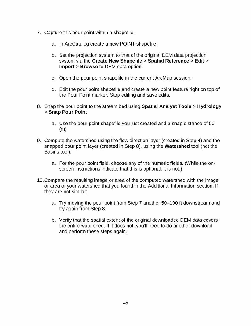
48

7. Capture this pour point within a shapefile.

a. In ArcCatalog create a new POINT shapefile.

b. Set the projection system to that of the original DEM data projection system via the Create New Shapefile > Spatial Reference > Edit > Import > Browse to DEM data option.

c. Open the pour point shapefile in the current ArcMap session.

d. Edit the pour point shapefile and create a new point feature right on top of

the Pour Point marker. Stop editing and save edits.

8. Snap the pour point to the stream bed using Spatial Analyst Tools > Hydrology > Snap Pour Point

a. Use the pour point shapefile you just created and a snap distance of 50

(m)

9. Compute the watershed using the flow direction layer (created in Step 4) and the snapped pour point layer (created in Step 8), using the Watershed tool (not the Basins tool).

a. For the pour point field, choose any of the numeric fields. (While the on-

screen instructions indicate that this is optional, it is not.)

10. Compare the resulting image or area of the computed watershed with the image or area of your watershed that you found in the Additional Information section. If they are not similar:

a. Try moving the pour point from Step 7 another 50–100 ft downstream and

try again from Step 8.

b. Verify that the spatial extent of the original downloaded DEM data covers the entire watershed. If it does not, you’ll need to do another download and perform these steps again.

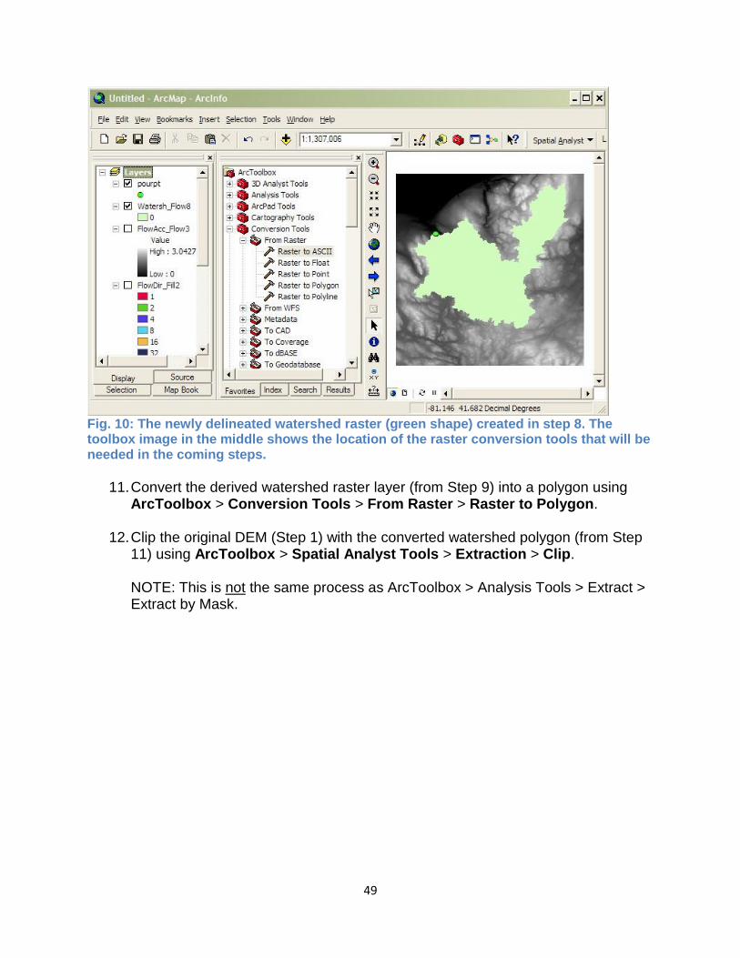
49

Fig. 10: The newly delineated watershed raster (green shape) created in step 8. The toolbox image in the middle shows the location of the raster conversion tools that will be needed in the coming steps.

11. Convert the derived watershed raster layer (from Step 9) into a polygon using

ArcToolbox > Conversion Tools > From Raster > Raster to Polygon.

12. Clip the original DEM (Step 1) with the converted watershed polygon (from Step 11) using ArcToolbox > Spatial Analyst Tools > Extraction > Clip.

NOTE: This is not the same process as ArcToolbox > Analysis Tools > Extract > Extract by Mask.

50

Fig. 11: ArcGIS screenshot of the DEM clipped to the shape of the delineated watershed (step 12). The toolbox shows the extraction tools used to clip the DEM.

13. Re-project the clipped DEM (from Step 12) to UTM meters using ArcToolbox >

Data Management Tools > Projections and Transformations > Raster > Project Raster.

a. The UTM zone is dependent on the project area. For UTM zones

guidance: https://pubs.usgs.gov/fs/2001/0077/report.pdf

b. Output coordinate system should be: NAD_1983 datum

c. Geographic transformation should be: left blank

d. Leave other values as defaults.

14. To calculate the area of the watershed, re-project the converted watershed layer (from step 11) following the directions from step 13. Select Open Attribute Table. Use the table tools to add a new field for area, then right-click on the added field and select Calculate Geometry. Select Area and square kilometers.

15. Export the clipped, re-projected DEM (from step 14) to ASCII format using

ArcToolBox > Conversion Tools > From Raster > Raster to ASCII.

16. In Windows Explorer, change the file type extension of the ASCII file (from Step 15) from .TXT to .DAT for use within i-Tree Hydro.

https://pubs.usgs.gov/fs/2001/0077/report.pdf

51

Appendix 2: Topographic Index Data

A Topographic Index (TI) is constructed using a 30-meter DEM as follows:

1. TI approximates spatial distribution of the depth to water table. It is calculated using the following formula:

𝑇𝐼 = 𝜆 = ln (𝛼

tan 𝛽) (𝐄𝐪𝐧. 𝟒)

where: α= specific catchment area defined = (# of upslope cells + 1) * grid cell length

tanβ = slope gradient defined as the rise over run along the steepest path from the cell center to its neighbor

2. This dataset was generated using a 30-meter resampled DEM. Output dataset

was 100-meter resolution. TI Histograms were generated in ESRI’s ArcGIS with the following input datasets: Topographic Index Raster, Zone Boundary Files (State, County, Place, gaged and HUC8 watersheds), and National Hydrography Dataset (NHD) high-res water bodies.

1. The NHD water bodies dataset was used to erase all portions of the zone boundary within a water body that crosses the outline of the zone boundary. This was only done for States, Counties and Places.

2. ArcGIS SpatialAnalyst Tools > Zonal > Tabulate Area was run to compute the

cross-tabulated area between the Topographic Index dataset and the zones in the area of interest boundary file (State, County, Place, gaged, and HUC8). This process outputs a table containing a record for each location with fields containing the total area of each pixel value.

3. ArcGIS SpatialAnalyst Tools > Zonal > Zonal Statistics As Table was run to

summarize the values (max, min, sum) of the TI raster within the zones of the boundary file (State, County, Place, gaged, and HUC8).

4. The range of TI values in each zone was split into 30 bins (or histogram classes)

and the number of pixels in each bin is calculated. For detailed instructions on how to create your own TI map, refer to this presentation: http://soilandwater.bee.cornell.edu/tools/TI.pdf

http://soilandwater.bee.cornell.edu/tools/TI.pdf

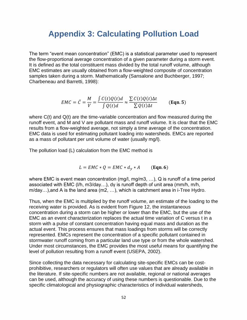
52

Appendix 3: Calculating Pollution Load The term “event mean concentration” (EMC) is a statistical parameter used to represent the flow-proportional average concentration of a given parameter during a storm event. It is defined as the total constituent mass divided by the total runoff volume, although EMC estimates are usually obtained from a flow-weighted composite of concentration samples taken during a storm. Mathematically (Sansalone and Buchberger, 1997; Charbeneau and Barretti, 1998):

𝐸𝑀𝐶 = 𝐶̅ =𝑀

𝑉=

∫ 𝐶(𝑡)𝑄(𝑡)𝑑

∫ 𝑄(𝑡)𝑑≈

∑ 𝐶(𝑡)𝑄(𝑡)∆𝑡

∑ 𝑄(𝑡)∆𝑡 (𝐄𝐪𝐧. 𝟓)

where C(t) and Q(t) are the time-variable concentration and flow measured during the runoff event, and M and V are pollutant mass and runoff volume. It is clear that the EMC results from a flow-weighted average, not simply a time average of the concentration. EMC data is used for estimating pollutant loading into watersheds. EMCs are reported as a mass of pollutant per unit volume of water (usually mg/l). The pollution load (L) calculation from the EMC method is

𝐿 = 𝐸𝑀𝐶 ∗ 𝑄 = 𝐸𝑀𝐶 ∗ 𝑑𝑦 ∗ 𝐴 (𝐄𝐪𝐧. 𝟔)

where EMC is event mean concentration (mg/l, mg/m3, …), Q is runoff of a time period associated with EMC (l/h, m3/day…), dγ is runoff depth of unit area (mm/h, m/h, m/day…),and A is the land area (m2, …), which is catchment area in i-Tree Hydro. Thus, when the EMC is multiplied by the runoff volume, an estimate of the loading to the receiving water is provided. As is evident from Figure 12, the instantaneous concentration during a storm can be higher or lower than the EMC, but the use of the EMC as an event characterization replaces the actual time variation of C versus t in a storm with a pulse of constant concentration having equal mass and duration as the actual event. This process ensures that mass loadings from storms will be correctly represented. EMCs represent the concentration of a specific pollutant contained in stormwater runoff coming from a particular land use type or from the whole watershed. Under most circumstances, the EMC provides the most useful means for quantifying the level of pollution resulting from a runoff event (USEPA, 2002). Since collecting the data necessary for calculating site-specific EMCs can be cost- prohibitive, researchers or regulators will often use values that are already available in the literature. If site-specific numbers are not available, regional or national averages can be used, although the accuracy of using these numbers is questionable. Due to the specific climatological and physiographic characteristics of individual watersheds,

53

agricultural and urban land uses can exhibit a wide range of variability in nutrient export (Beaulac and Reckhow 1982).

Fig. 12: Interstorm variation in pollutographs and EMCs.

To understand and control urban runoff pollution, the U.S. Congress included the establishment of the Nationwide Urban Runoff Program (NURP) in the 1977 Amendments of the Clean Water Act (PL 95-217). The U.S. Environmental Protection Agency developed the NURP to expand the state knowledge of urban runoff pollution by applying research projects and instituting data collection in selected urban areas throughout the country. In 1983, the U.S. Environmental Protection Agency published the results of the NURP, which nationally characterizes urban runoff for 10 standard water quality pollutants, based on data from 2,300 station-storms at 81 urban sites in 28 metropolitan areas. Two important conclusions from NURP investigations:

• The variance of the EMCs when data from sites are grouped by land use type or geographic region is so great that difference in measures of central tendency among groups statistically are not significant;

• Statistically, the entire sample of EMCs, and the medians of all EMCs among

sites, are lognormally distributed. Thus the numbers in Table 10 do not distinguish between different urban land use types. Subsequently, the USGS created another urban stormwater runoff base (Driver et al, 1985), based on data measured through mid-1980s for over 1,100 stations at 97 urban sites located in 21 metropolitan areas. Additionally, many major cities in the United States collected urban runoff quality data as part of the application requirements for stormwater discharge permits under the National Pollutant Discharge Elimination System (NPDES). The NPDES data are from over 30 cities and more than 800 station-storms for over 150 parameters (Smullen et al, 1999).

Co

nc

en

tra

tio

n C

54

The data from the three sources (NURP, USGS, and NPDES) were used to compute new estimates of EMC population means and medians for the 10 pollutants with many more degrees of freedom than were available to the NURP investigators (Smullen et al, 1999). A “pooled” mean was calculated representing the mean of the total population of sample data. The NURP and pooled mean EMCs for the 10 constitutes are listed in Table 10 (Smullen et al, 1999). NURP or pooled mean EMCs were selected because they are based on field data collected from thousands of storm events. These estimates are based on nationwide data, however, so they do not account for regional variation in soil types, climate, and other factors. Table 10. National Pooled EMCs and NURP EMCs

Constituent Data

a

source

EMCs (mg/L) No. of

events Mean Median

Total suspended solids: TSS Pooled 78.4 54.5 3047

NURP 17.4 113 2000

Biochemical oxygen demand: BOD5 Pooledb

14.1 11.5 1035

NURP 10.4 8.39 474

Chemical oxygen demand: COD Pooled 52.8 44.7 2639

NURP 66.1 55 1538

Total phosphorus: TP Pooled 0.315 0.259 3094

NURP 0.337 0.266 1902

Soluble phosphorus: soluble P Pooled

c 0.129 0.103 1091

NURP 0.1 0.078 767

Total Kjeldhal nitrogen: TKN Pooled 1.73 1.47 2693

NURP 1.67 1.41 1601

Nitrite and nitrate: NO2 and NO3 Pooled 0.658 0.533 2016

NURP 0.837 0.666 1234

Copper: Cu Pooled 0.0135 0.0111 1657

NURP 0.0666 0.0548 849

Lead: Pb Pooled 0.0675 0.0507 2713

NURP 0.175 0.131 1579

Zinc: Zn Pooled 0.162 0.129 2234

NURP 0.176 0.140 1281

a Pooled data sources include: NURP, USGS, NPDES b No BOD5 data available in the USGS dataset; pooled includes NURP+NPDES c No TS data available in NPDES dataset; pooled includes NURP+USGS

(Source: Smullen et al., 1999)

55

For i-Tree Hydro, the pooled median and mean EMC value for each pollutant (Table 10) are applied to the runoff regenerated from pervious and impervious surface flow, not the baseflow values, to estimate effects on pollutant load across the entire modeling time frame. All rain events are treated equally using the EMC value, which means some events may be overestimated and others underestimated. In addition, local management actions (e.g., street sweeping) can affect these values. However, across the entire season, if the EMC value is representative of the watershed, the estimate of cumulative effects on water quality should be relatively accurate. Accuracy of pollution estimates will be increased by using locally derived coefficients. It is not known how well the national EMC values represent local conditions.

56

Appendix 4: International Support We recognize that users outside of the United States may wish to experiment with i-Tree Hydro. It should be noted that the application and model have been built with specific U.S. data in mind. Users in other countries will need to find and format appropriate data to meet the requirements of i-Tree Hydro. This can be a difficult process; please review the following suggestions for guidance. Please also periodically visit the online forums at forums.itreetools.org to see if other users have posted additional information. Additional support for users outside the U.S. may be added in future versions of i-Tree.

1. A DEM file should be created for the project with GIS software. See Appendix 1 for more information on how to do this for a watershed using ArcGIS.

2. Land cover data can be obtained using i-Tree Canopy or other methods listed in Gathering Data > Land cover parameters.

3. The user should select a U.S. location similar to the project location based on

latitude and elevation. The parameters affected by project location are used to process weather data (specifically, project location defines latitude; longitude; elevation; GMTOffset; Leaf-on/off; albedo; ozone; coeffA; coeffC; and coeffPHI for weather pre-processing).

4. Weather data is required with the following fields:

• DIR (wind direction) • SPD (wind speed in mph) • CLG (cloud ceiling – lowest opaque layer with 5/8 or greater coverage, in

hundreds of feet) • SKC (sky cover) • TEMP (temperature in Fahrenheit) • DEWP (dew point in Fahrenheit) • STP (station pressure in millibars; can be converted from ALT) or • ALT (altimeter setting in inches; can be converted to STP) • PCP01 (hourly precipitation in inches and hundredths)

The weather file must be a fixed-width text file. The model will interpolate gaps in the data, though they should be kept under 72 hours. This data should be in GMT. Example: USAF WBAN YR--MODAHRMN DIR SPD GUS CLG SKC L M H VSB WW WW WW W TEMP DEWP SLP ALT STP MAX MIN

PCP01 PCP06 PCP24 PCPXX SD 703080 25713 200401010953 220 18 *** 722 SCT * * * 10.0 00 ** ** * 36 26 1019.0 30.09 ****** *** *** 0.00 ***** ***** ***** ** 703080 25713 200401011053 220 18 23 47 BKN * * * 7.0 00 ** ** * 36 27 1020.0 30.12 ****** *** *** 0.00 ***** ***** ***** **

http://forums.itreetools.org/

57

5. Stream gage data* is required if the user wants to calibrate the model. The file must be tab-delimited and contain headers similar to the U.S. data.

Example: # column column definition # ----------- ----------------------------------------- # site_no USGS site identification number # date_time date and time in format (YYYYMMDDhhmmss) # tz_cd time zone # dd internal USGS sensor designation (''data descriptor'') # accuracy_cd accuracy code # 0 - A daily mean discharge calculated from the instantaneous # data on this day is 0.01 cubic feet per second # or less and the published daily mean is zero. # 1 - A daily mean discharge calculated from the instantaneous # data on this day matches the published daily mean # within 1 percent. # 2 - A daily mean discharge calculated from the instantaneous # data on this day matches the published daily mean # from greater than 1 to 5 percent. # 3 - A daily mean discharge calculated from the instantaneous # values on this day matches the published daily mean # from greater than 5 to 10 percent. # 9 - The instantaneous value is considered correct by the # collecting USGS Water Science Center. A published daily # mean value does not exist and/or no comparison was made. # value discharge in cubic feet per second # # site_no date_time tz_cd dd accuracy_cd value prec remark 15N 14N 6S 2N 5S 16N 1S 1S 06710150 20070101000000 MST 2 1 2.4 2

06710150 20070101001500 MST 2 1 2.7 2 06710150 20070101003000 MST 2 1 2.7 2 06710150 20070101004500 MST 2 1 2.9 2

* NOTE: The date_time value for the streamflow file should match the local time of the project location you specified above. Raw stream gage data are expected to be in local time, while raw weather data are expected to be in UTC and are automatically converted to local time upon processing in order to synchronize the two files.

58

Appendix 5: Glossary Alternative Case: The scenario being modeled at the same time as the base case; the

two are directly compared in several of the model outputs. The alternative case, defined in Step 4, is based on the base case but has different land cover distribution. Often the alternative case is set up to model the addition of green infrastructure, alternative management schemes, or the planting of trees.

Base Case: The current or initial situation to be modeled. The base case typically

represents current watershed or project area parameters to allow for calibration of the model.

Base Flow: The primary source of water during periods of low flow. Usually

groundwater fed, but also fueled by water slowly draining from the subsurface into the river over time. Simply put, base flow is defined as the portion of surface water supplied by groundwater.

Depth of Root Zone: The average depth to which roots of a plant penetrate into the soil

for development of its plant root system. Digital Elevation Model (DEM): A digital model or 3D representation of terrain,

showing elevation, often represented as a grid containing z values. Directly Connected Impervious Area (DCIA): The portion of impervious cover that

drains directly to a stream or any of its tributaries. “Drains directly” describes a

situation where precipitation that falls on a portion of the watershed’s impervious

cover is conveyed, overland or through a storm sewer network, directly into the

stream or its tributaries.

Evaporation: The vaporization of a liquid into a gas. Occurs on the surface of that liquid. In the hydrologic cycle, this means the vaporization of water from lakes, rivers, etc. into the atmosphere.

Evapotranspiration: The transport of water into the atmosphere from surfaces such as

soil, vegetation (transpiration), wet canopy surfaces, and vegetation-covered water surface in wetlands.

Event Mean Concentration (EMC): The flow-proportional average concentration of a

given pollutant during a storm event. Measured in units of mass per volume (usually milligrams per liter), EMC can be multiplied by actual flow to estimate the mass of pollutants entering a body of water.

Groundwater Recharge: The process of water moving from the surface to the water

table. Maintains the supply of fresh water that flows through the groundwater system to wells, streams, springs, and wetlands.

59

Hydrologic Cycle: The water cycle. Describes the continuous movement of water on,

above, and below the surface of the Earth. Represented as a figure in the i-Tree Hydro program. Specific terms defined in Glossary.

Impervious Cover: Roads, buildings, parking lots and other hard surfaces that prevent

rainfall from naturally infiltrating into the soil. Impervious Depression Storage: The impervious area depression storage found

across the watershed. This depth is filled before runoff generation from the impervious area begins. Examples: potholes, low-lying impervious areas (sinks), street curbs that are blocked by debris, etc.

Infiltration: The process by which water on the ground surface enters the soil. Infiltration Excess Overland Flow: also known as Hortonian Flow. Occurs when water

enters a soil system faster than the soil can absorb or move it, such as when precipitation exceeds the infiltration capacity of the soil.

Infiltration Rate: a measure of the rate at which soil is able to absorb rainfall or

irrigation. Initial Soil Saturation: The amount of water storage in the soil at the start of the

simulation. This affects infiltration. An initial soil saturation value of 0% represents soil that is absolutely dry; an initial soil saturation value of 100% represents soil that is completely saturated.

Leaf Area Index (LAI): The one sided green leaf area per unit canopy area in broadleaf

canopies or the projected needleleaf area per unit canopy area in needle canopies. Standing in a 1-meter square area, looking up into the tree canopy, the LAI represents the surface area (1-sided) of the leaves present directly above this 1 meter square area. Typical LAI values range from 1-7, representing 1-7 square meters of leaf area (1-sided) above this 1-meter square area. Shrub and herbaceous LAI are typically less than Tree LAI due to the decreased canopy size and density of typical shrub and herbaceous canopies. LAI can be calculated as the total one sided green leaf area (m2), divided by the total canopy area of the study (m2, total study area multiplied by the percent tree cover).

Leaf On Day: The day of the year where the leaves begin the transition from the

minimum LAI, experienced by deciduous trees in the winter (represented by the bark area index), to the maximum LAI, which represents a full canopy in the spring and summer.

60

Leaf Off Day: The day of the year where the leaves end the transition from the maximum LAI, which represents a full canopy in the spring and summer, to the minimum LAI, experienced by deciduous trees in the winter (represented by the bark area index).

Leaf Storage: The maximum water depth that a single leaf in the tree or shrub canopy

can hold. Intercepted precipitation that increases the depth of water stored on leaf above this threshold is shed as throughfall in the interception and throughfall processes.

Leaf Transition Period: The number of days for the leaves to transition from the

minimum LAI experienced by deciduous trees in the winter (represented by the bark LAI) to the maximum LAI that represents a full canopy in the spring and summer.

Percolation: The movement of water through the soil profile Pervious: The quality of allowing water to pass through. In the context of stormwater,

pervious generally implies allowing water to pass into subsurface zones. For example, soil or herbaceous cover generally allows water to percolate into subsurface flows and are therefore considered pervious.

Pervious Depression Storage: The pervious area depression storage found across

the watershed. This depth is filled before runoff generation from the pervious area begins. Examples: low-lying pervious areas (sinks), depressions caused by landscaping or tree growth, areas of compacted soil found in parks, fields, etc.

Precipitation: Any product of the condensation of atmospheric water that falls under

gravity. Mainly rain and snow. Runoff: The water flow that occurs when the soil is infiltrated to full capacity and excess

water from precipitation, meltwater, or other sources flows over land. Also occurs on impervious surfaces, as these have no infiltration capacity.

Saturated Zone: The soil layer where all pores are filled with water. Saturation Excess Overland Flow: Occurs when the soil is saturated and depression

storage is filled, in which case any additional precipitation or irrigation immediately causes runoff.

61

Scale Parameter of Power Function: The power used in the power function

formulation of the Green and Ampt infiltration equation used in i-Tree Hydro. These equations (below) model the decay of infiltration rates as infiltration occurs. Refer to Wang, Endreny, and Nowak, 2008 for more information.

𝐼 =𝑑𝐼

𝑑𝑡=

∆𝜓 + 𝑍

∫𝑑𝑧

𝐾𝑧

𝑧=𝑧

𝑧=0

(𝐄𝐪𝐧. 𝟕)

𝐾𝑧 = 𝐾0(1 − 𝑓𝑧)𝑛 (𝐄𝐪𝐧. 𝟖)

Scale Parameter of Soil Transmissivity: A scaling parameter describing the change

of soil transmissivity with soil depth. It affects saturated zone baseflow recession. It is estimated through knowledge of the watershed recession rates, which relate to unsaturated zone maximum water storage depth, and optimized in its role as a calibrated parameter. The equation is below. Refer to Wang, Endreny, and Hasset, 2006 for more information.

𝑇𝑧 = 𝑇0(1 − 𝑠𝑚⁄ )2 (𝐄𝐪𝐧. 𝟗)

Shrub Bark Area Index: The minimum LAI, represented by leafless canopy coverage

of deciduous shrubs in the winter, which is defined as the shrub bark area index. Surface Hydraulic Conductivity: Controls infiltration rates. For horizontal flow, this is

the maximum rate water flows in the unsaturated zone, but for vertical flow at infiltration, it is the minimum infiltration rate. The decrease of hydraulic conductivity with depth follows exponential law or power law profiles. It is estimated from soil physical properties used in Green-Ampt lookup tables.

Throughfall: The process which describes how wet leaves shed excess water onto the

ground surface. Time Constant for Surface Flow: Alpha: This parameter controls the distribution of

flows in the surface hydrograph. It is calibrated as part of the modeling process. The equation is below. Refer to Yang and Endreny, 2013 for more information.

𝛼 =4𝐷

𝑐2 (𝐄𝐪𝐧. 𝟏𝟎)

Time Constant for Surface Flow: Beta: This parameter controls the distribution of

flows in the surface hydrograph. It is calibrated as part of the modeling process. The equation is below. Refer to Yang and Endreny, 2013 for more information.

𝛽 =𝑥2

4𝐷 (𝐄𝐪𝐧. 𝟏𝟏)

62

Topographic Index (TI): A grid of indices derived from a DEM that assumes

topography drives flow. It is calculated using the upslope contributing area (α) and the slope of the grid cell (β) (see equation below). TI influences flow accumulation, soil moisture, distribution of saturation zones, depth of water table, evapotranspiration, thickness of soil horizons, organic matter, pH, silt and sand content, and plant cover distribution.

𝜆 = ln (𝛼

tan 𝛽) (𝐄𝐪𝐧. 𝟏𝟐)

Transmissivity at Saturation: Transmissivity of the saturated zone, controls base flow

rates and represents product of saturated depth and hydraulic conductivity in the saturated zone. It is estimated by physical knowledge of depth and conductivity which can be collected from inputs.

Tree Canopy: The upper layer of the tree leaves, formed by mature tree crowns. Tree Bark Area Index: The minimum LAI, represented by leafless canopy coverage of

deciduous trees in the winter, which is defined as the tree bark area index. Unsaturated Zone: Also known as the Vadose Zone. The soil above the groundwater

table, which has both water and air in the soil pores. Unsaturated Zone Time Delay: Controls the travel time for unsaturated zone water to

move to the saturated zone. It is estimated from knowledge of the soil’s hydraulic conductivity and soil layer depths and then calibrated as part of the modeling process.

Watershed: The area of land where all of the water that drains off of it or is under it

goes into the same discharge point. Wetting Front Suction: Controls the maximum infiltration rates. It is used to describe

the rate at which water is pulled into the soil when it is dry during the early part of the infiltration process. It is estimated from soil physical properties used in Green-Ampt lookup tables.

Wetted Moisture Content: The difference between the initial volumetric moisture

content value below the infiltration wetting front and the volumetric water content within the wetting front (unitless, ranges from 0 to 1.0). In other words, it is the difference between the soil moisture content at saturation and the initial (typical) soil moisture content. It affects the infiltration rate. It is estimated from soil physical properties used in Green-Ampt lookup tables.

63

Appendix 6: Additional Resources i-Tree Hydro Documents Main i-Tree Hydro website: http://www.itreetools.org/hydro/index.php i-Tree Hydro FAQs: https://forums.itreetools.org/viewforum.php?f=35 Atlanta i-Tree Hydro Workshop presentation slides (2014):

http://www.itreetools.org/resources/presentations/GT_iTree_Hydro_workshop031214.pdf

i-Tree Version 5 webinar: Quantifying the Benefits of Trees (2013):

http://youtu.be/sw6cxkO1K5k?t=14m40s Journal Articles

Power function decay of hydraulic conductivity for a TOPMODEL-based_infiltration

routine. Wang, Endreny, and Hasset, 2006: http://www.itreetools.org/hydro/resources/Power_function_decay_of_hydraulic_conductivity_TOPMODEL_based_infiltration_routine.pdf

Mechanistic simulation of tree effects in an urban water balance model. Wang, Endreny,

and Nowak, 2008: http://www.itreetools.org/hydro/resources/Hydro%20Model%20Methodology.pdf

i-Tree Hydro: Snow Hydrology Update for the Urban Forest Hydrology Model. Yang,

Endreny, and Nowak, 2011: http://www.itreetools.org/hydro/resources/iTree_Hydro_Snow_Hydrology_Model_Update_JAWRA.pdf

Watershed hydrograph model based on surface flow diffusion. Yang and Endreny,

2013: http://www.itreetools.org/hydro/resources/Watershed_hydrograph_model_based_on_surface_flow_diffusion.pdf

Surface and Upper Weather Pre-processor for i-Tree Eco and Hydro. Hirabayashi and

Endreny, 2013: http://www.itreetools.org/eco/resources/Surface_weather_and_upper_air_preprocessor_description.pdf

ArcGIS Help Main website: http://www.esri.com/software/arcgis

http://www.itreetools.org/hydro/index.php

https://forums.itreetools.org/viewforum.php?f=35



http://youtu.be/sw6cxkO1K5k?t=14m40s

http://www.itreetools.org/hydro/resources/Power_function_decay_of_hydraulic_conductivity_TOPMODEL_based_infiltration_routine.pdf

http://www.itreetools.org/hydro/resources/Power_function_decay_of_hydraulic_conductivity_TOPMODEL_based_infiltration_routine.pdf

http://www.itreetools.org/hydro/resources/Hydro%20Model%20Methodology.pdf

http://www.itreetools.org/hydro/resources/iTree_Hydro_Snow_Hydrology_Model_Update_JAWRA.pdf

http://www.itreetools.org/hydro/resources/iTree_Hydro_Snow_Hydrology_Model_Update_JAWRA.pdf

http://www.itreetools.org/hydro/resources/Watershed_hydrograph_model_based_on_surface_flow_diffusion.pdf

http://www.itreetools.org/hydro/resources/Watershed_hydrograph_model_based_on_surface_flow_diffusion.pdf

http://www.itreetools.org/eco/resources/Surface_weather_and_upper_air_preprocessor_description.pdf

http://www.itreetools.org/eco/resources/Surface_weather_and_upper_air_preprocessor_description.pdf

http://www.esri.com/software/arcgis

64

Main help and resources page: http://resources.arcgis.com/en/help/ Main help forum: http://forums.arcgis.com/ Data Sources

Map Data USGS DEM website: http://viewer.nationalmap.gov/viewer/ UTM zones guidance: http://pubs.usgs.gov/fs/2001/0077/report.pdf USDA NRCS Geospatial Data Gateway: http://datagateway.nrcs.usda.gov/ NYS GIS Clearinghouse: http://gis.ny.gov/gateway/mg/?nysgis= HUC watersheds: http://water.usgs.gov/GIS/huc.html GAGES-II dataset of USGS stream gage basins:

http://water.usgs.gov/GIS/metadata/usgswrd/XML/gagesII_Sept2011.xml Soils Data

USDA NRCS Web Soil Survey to inform local soil parameters:

http://websoilsurvey.sc.egov.usda.gov/App/HomePage.htm Stream Data USGS stream gage data: http://maps.waterdata.usgs.gov/mapper/index.html EPA’s Waters website - WATERS Data 1.5(Vector).kmz file:

http://water.epa.gov/scitech/datait/tools/waters/tools/waters_kmz.cfm i-Tree Hydro Gauging Stations 2005 - A zip file containing a Google Earth (.kmz) file

of stream gauging stations available in i-Tree Hydro: http://www.itreetools.org/hydro/resources/iTree_Hydro_Gauging_Stations_2005.zip

i-Tree Hydro model raw stream data example:

http://www.itreetools.org/hydro/resources/Hydro_stream_data_example.txt

http://resources.arcgis.com/en/help/

http://forums.arcgis.com/

http://viewer.nationalmap.gov/viewer/

http://pubs.usgs.gov/fs/2001/0077/report.pdf

http://datagateway.nrcs.usda.gov/

http://gis.ny.gov/gateway/mg/?nysgis=

http://water.usgs.gov/GIS/huc.html

http://water.usgs.gov/GIS/metadata/usgswrd/XML/gagesII_Sept2011.xml

http://websoilsurvey.sc.egov.usda.gov/App/HomePage.htm

http://maps.waterdata.usgs.gov/mapper/index.html

http://water.epa.gov/scitech/datait/tools/waters/tools/waters_kmz.cfm

http://www.itreetools.org/hydro/resources/iTree_Hydro_Gauging_Stations_2005.zip

http://www.itreetools.org/hydro/resources/iTree_Hydro_Gauging_Stations_2005.zip

http://www.itreetools.org/hydro/resources/Hydro_stream_data_example.txt

65

Weather Data

NOAA Climate Data Online, our source of raw weather data (from the Intergrated

Surface Database, Hourly Precipitation records): http://www.ncdc.noaa.gov/cdo-web/

i-Tree Hydro model raw weather data example:

http://www.itreetools.org/hydro/resources/Hydro_weather_data_example.txt i-Tree Hydro weather abbreviation codes:

http://www.itreetools.org/hydro/resources/ish-abbreviated.txt Other Data Excel VBA Parameter Conversion macro: http://www.esf.edu/ere/endreny/GI-

iTree/Parameter%20Conversion.xlsm i-Tree Hydro DEM file example: http://www.itreetools.org/hydro/resources/Hydro_DEM_data_example.dat i-Tree Hydro TI file example: http://www.itreetools.org/hydro/resources/Hydro_TI_data_example.dat

Other Resources Main i-Tree website: http://www.itreetools.org/ i-Tree support page: www.itreetools.org/support i-Tree Canopy main page: http://www.itreetools.org/canopy/index.php i-Tree Canopy (8) cover class version for i-Tree Hydro:

http://www.itreetools.org/hydro/resources/Hydro_Canopy_survey_cover_classes_example1_long

i-Tree Workshop Information: http://www.itreetools.org/resources/training/index.php Information about green infrastructure techniques:

http://www.esf.edu/ere/endreny/GICalculator/TechniquesHome.html Runoff calculator: http://www.esf.edu/ere/endreny/GICalculator/RunoffHome.html Topographic Index information and creation:


http://www.ncdc.noaa.gov/cdo-web/

http://www.itreetools.org/hydro/resources/Hydro_weather_data_example.txt

http://www.itreetools.org/hydro/resources/ish-abbreviated.txt

http://www.esf.edu/ere/endreny/GI-iTree/Parameter%20Conversion.xlsm

http://www.esf.edu/ere/endreny/GI-iTree/Parameter%20Conversion.xlsm

http://www.itreetools.org/hydro/resources/Hydro_DEM_data_example.dat

http://www.itreetools.org/hydro/resources/Hydro_TI_data_example.dat


http://www.itreetools.org/support

http://www.itreetools.org/canopy/index.php



http://www.itreetools.org/resources/training/index.php

http://www.esf.edu/ere/endreny/GICalculator/TechniquesHome.html

http://www.esf.edu/ere/endreny/GICalculator/RunoffHome.html


66

References

Beaulac, M. N., and Reckhow, K. H. 1982. An examination of land use-nutrient export relationships. Water Resources Bulletin, 18(6), 1013-1024. Charbeneau, R. J., and Barretti, M. 1998. Evaluation of methods for estimating stormwater pollutant loads. Water Environ Res. 70: 1295-1302. Chesapeake Stormwater Network. 2009. CSN Technical Bulletin No. 4: Technical Support for theBay-wide Runoff Reduction Method Version 2.0. www.chesapeakestormwater.net/documents/research-files/CSN20TB20No.2042020Baywide20Runoff20Reduction20Method1.pdf Driver, N. E., Mustard, M. H., Rhinesmith, R. B., and Middelburg, R. F. 1985. U.S. Geological Survey urban-stormwater data base for 22 metropolitan areas throughout the United States. United States Geological Survey, Open-File Report 85-337, Lakewood, CO. Lindsay JB. 2016. Whitebox GAT: A case study in geomorphometric analysis. Computers & Geosciences, 95: 75-84. DOI: 10.1016/j.cageo.2016.07.003 Schueler, T. 2009. Guidance for meeting NPDES Permit Requirement in Montgomery County, MD. Sansalone, J. J., and Buchberger, S.G. 1997. Partitioning and first flush of metals in urban roadway storm water. J Environ Eng ASCE 123: 134-143. Smullen, J. T., Shallcross,A. L., and Cave, K. A. 1999. Updating the U.S. nationwide urban runoff quality database. Water Science Technology 39(12), 9-16. Sutherland. 2000. Methods for Estimating Effective Impervious Cover. Article 32 in The Practice of Watershed Protection, Center for Watershed Protection, Ellicott City, MD. U.S. Environmental Protection Agency (USEPA). 1983. Results of the Nationwide Urban Runoff Program: Volume I – final report. U.S. Environmental Protection Agency, PB84-185552, Washington, DC. U.S. Environmental Protection Agency (USEPA). 2002. Urban Stormwater BMP

Performance Monitoring, A Guidance Manual for Meeting the National Stormwater

BMP Database Requirements.

U.S. Environmental Protection Agency (USEPA). 2011a. Estimating Change in

Impervious Area (IA) and Directly Connected Impervious Areas (DCIA) for

http://www.chesapeakestormwater.net/documents/research-files/CSN20TB20No.2042020Baywide20Runoff20Reduction20Method1.pdf

http://www.chesapeakestormwater.net/documents/research-files/CSN20TB20No.2042020Baywide20Runoff20Reduction20Method1.pdf

67

Massachusetts Small MS4 Permit. USEPA Small MS4 Permit Technical Support

Document.

U.S. Environmental Protection Agency (USEPA). 2011b. Estimating Change in

Impervious Area (IA) and Directly Connected Impervious Areas (DCIA) for New

Hampshire Small MS4 Permit. USEPA Small MS4 Permit Technical Support

Document.

Wang, J., Endreny, T. A., and Hassett, J. M. 2006. Power function decay of hydraulic conductivity for a TOPMODEL-based infiltration routine. Hydrol. Process. 20, 3825 – 3834. DOI: 10.1002/hyp.6159 Wang, J., Endreny, T. A., and Nowak, D. J. 2008. Mechanistic simulation of tree effects in an urban water balance model. JAWRA. 44(1), 75-85. Wolock, D. M., and McCabe, G. J. 2000. Differences in topographic characteristics computed from 100- and 1000-m resolution digital elevation model data. Hydrol. Process. 14, 987±1002. Wolock, D. M., and Price, C. V. 1994. Effects of digital elevation model map scale and data resolution on a topography-based watershed model. Water Resources Research, 30(11), 3041-3052. Yang, Y and Endreny, T. A.. 2013. Watershed hydrograph model based on surface flow diffusion. Water Resources Research. 49, 507–516, doi:10.1029/2012WR012186.