Embed Size (px)
Citation preview

User manual
TReCCA Analyser Version 4.0
Time-Resolved Cell Culture Assay Analyser
Julia Lochead1,2, Julia Schessner1
1 Universität Heidelberg, Institut für Pharmazie und molekulare Biotechnologie,
INF364, 69120 Heidelberg, Germany
2 Hochschule Mannheim, Institut für analytische Chemie,
Paul-Wittsack-Straÿe 10, 68163 Mannheim, Germany
June 30, 2015


Contents
1 Preface 5
2 Intended use 7
3 Installation guide 9
3.1 Downloading R and the complementary packages . . . . . . . . . . . . . . 9
3.2 Running the TReCCA Analyser . . . . . . . . . . . . . . . . . . . . . . . . 12
4 Quick guide 15
5 Detailed user guide 17
5.1 Data input . . . . . . . . . . . . . . . . . . . . . . . . . . . . . . . . . . . . 17
5.1.1 Required format . . . . . . . . . . . . . . . . . . . . . . . . . . . . . 17
5.1.2 Data layout . . . . . . . . . . . . . . . . . . . . . . . . . . . . . . . 18
5.1.3 Cutting borders . . . . . . . . . . . . . . . . . . . . . . . . . . . . . 19
5.1.4 File import . . . . . . . . . . . . . . . . . . . . . . . . . . . . . . . 20
5.2 Labels & colours . . . . . . . . . . . . . . . . . . . . . . . . . . . . . . . . 21
5.2.1 Template layout . . . . . . . . . . . . . . . . . . . . . . . . . . . . . 21
5.2.2 Filling the template automatically . . . . . . . . . . . . . . . . . . . 22
5.2.3 Saving and loading . . . . . . . . . . . . . . . . . . . . . . . . . . . 23
5.2.4 Excluding data from the analysis . . . . . . . . . . . . . . . . . . . 23
5.3 Analysis options . . . . . . . . . . . . . . . . . . . . . . . . . . . . . . . . . 23
5.3.1 Basic data formatting . . . . . . . . . . . . . . . . . . . . . . . . . 24
5.3.2 Average and standard deviation . . . . . . . . . . . . . . . . . . . . 26
5.3.3 Normalisation . . . . . . . . . . . . . . . . . . . . . . . . . . . . . . 26
5.3.4 OxoDish sensor calibration . . . . . . . . . . . . . . . . . . . . . . . 27
5.3.5 OxoPlate oxygen conversion . . . . . . . . . . . . . . . . . . . . . . 27
5.3.6 HydroPlate pH conversion . . . . . . . . . . . . . . . . . . . . . . . 29
5.3.7 Data smoothing . . . . . . . . . . . . . . . . . . . . . . . . . . . . . 30
5.3.8 Numerical slope . . . . . . . . . . . . . . . . . . . . . . . . . . . . . 31
5.3.9 Oxygen consumption . . . . . . . . . . . . . . . . . . . . . . . . . . 32
5.3.10 Oxygen consumption calibration . . . . . . . . . . . . . . . . . . . . 33
5.3.11 IC50 determination . . . . . . . . . . . . . . . . . . . . . . . . . . . 35
3

Contents
5.4 Graph options . . . . . . . . . . . . . . . . . . . . . . . . . . . . . . . . . . 37
5.4.1 General . . . . . . . . . . . . . . . . . . . . . . . . . . . . . . . . . 37
5.4.2 Axes . . . . . . . . . . . . . . . . . . . . . . . . . . . . . . . . . . . 38
5.5 Run analysis . . . . . . . . . . . . . . . . . . . . . . . . . . . . . . . . . . . 38
5.5.1 Graph output . . . . . . . . . . . . . . . . . . . . . . . . . . . . . . 39
5.5.2 Data output . . . . . . . . . . . . . . . . . . . . . . . . . . . . . . . 42
5.5.3 Import/export settings . . . . . . . . . . . . . . . . . . . . . . . . . 43
5.5.4 Import/export R-data . . . . . . . . . . . . . . . . . . . . . . . . . 44
6 Technical details 45
6.1 Average and standard deviation . . . . . . . . . . . . . . . . . . . . . . . . 45
6.2 Normalisation . . . . . . . . . . . . . . . . . . . . . . . . . . . . . . . . . . 45
6.3 OxoDish sensor calibration . . . . . . . . . . . . . . . . . . . . . . . . . . . 45
6.3.1 Step 1: Homogenising the sensor read-outs of each plate . . . . . . 46
6.3.2 Step 2: Setting the average read-out to a de�ned target . . . . . . . 47
6.4 OxoPlate oxygen conversion . . . . . . . . . . . . . . . . . . . . . . . . . . 47
6.5 HydroPlate pH conversion . . . . . . . . . . . . . . . . . . . . . . . . . . . 47
6.6 Data smoothing . . . . . . . . . . . . . . . . . . . . . . . . . . . . . . . . . 48
6.7 Numerical slope . . . . . . . . . . . . . . . . . . . . . . . . . . . . . . . . . 48
6.8 Oxygen consumption . . . . . . . . . . . . . . . . . . . . . . . . . . . . . . 48
6.9 Oxygen consumption calibration . . . . . . . . . . . . . . . . . . . . . . . . 49
6.10 IC50 determination . . . . . . . . . . . . . . . . . . . . . . . . . . . . . . . 50
7 Trouble shooting 51
7.1 Error messages . . . . . . . . . . . . . . . . . . . . . . . . . . . . . . . . . 51
7.2 R console . . . . . . . . . . . . . . . . . . . . . . . . . . . . . . . . . . . . 51
4 TReCCA Analyser user manual
1 Preface
We thank you for choosing the TReCCA Analyser for your time-resolved data. The aim
of this manual is to provide you with an overview of the functionalities of the program
and a course of action in the case of errors. This manual does not claim to be complete
and we welcome any ideas for its improvement.
An article about the TReCCA Analyser has been published in the open access and
peer-reviewed journal PLOS ONE (Lochead et al., 10(6):e0131233, 2015). Please refer
to this publication for a more detailed explanation of the justi�cation of some of the
proposed analysis steps and for a quick illustration of the possibilities of the program.
For more speci�c information on the actual code of the program or for its further
implementation please refer to the code of the TReCCA Analyser which is freely accessible
on the website of our research institute in Heidelberg:
http://www.uni-heidelberg.de/fakultaeten/biowissenschaften/ipmb/biologie/
woel�/Research.html.
If you wish to discover the use of the program through a practical example, you may
also refer to our tutorials (also available on our website). They will guide you through
di�erent analysing exercises that will exemplify the use of the program.
We wish you an enjoyable reading!
5


2 Intended use
The TReCCA Analyser is conceived to facilitate, speed up and intensify the analysis
and representation of your time-resolved data, more speci�cally in the case of cell cul-
ture assays. Without having to type any formula, it will perform at wish the following
calculations:
- Control condition normalisation.
- Technical replicate averaging and standard deviation calculation.
- Smoothing and slope calculation of the data in order to obtain the rate of change.
- IC50/EC
50determination of a substance in a time-resolved fashion.
In the particular case of an oxygen measurement over time, where a model of linear
di�usion of oxygen into cell culture well plates applies, this program can convert the
oxygen values measured to the actual oxygen consumption of the cell culture.
In the even more particular case of using the commercially available 24-well oxygen
sensor plate, the OxoDish (PreSens Precision Sensing GmbH, Germany), this program
will recalibrate the 24 oxygen sensors at the beginning of the experiment making the
read-out more homogeneous.
For the users of the commercially available 96-well pH or oxygen sensor plates, respec-
tively the HydroPlate or OxoPlate (PreSens Precision Sensing GmbH, Germany), this
program will convert the relative �uorescence intensity data to respective pH or oxygen
values.
The results of all these calculations will be automatically plotted using a simple tem-
plate and allowing an easy, fast and reproducible visualisation of the data. The graphs
produced are highly customisable: titles, axis description, legend content as well as sizes
and colours, exportation format... can all be modi�ed as wished.
The TReCCA Analyser is of course not restricted to the analysis of the results of
cell culture assays and can be used for any time-resolved data that need to be averaged,
normalised, derivated and plotted.
7


3 Installation guide
The TReCCA Analyser runs on every system which is compatible with the freely acces-
sible statistical analysis software R 1, as long as the packages described hereafter are also
available on the computer. Some details of the appearance of the program may vary from
one system to the other. In order to use the program, R and the corresponding packages
have to be downloaded to the computer, as well as the GTK+ widget toolkit. The pro-
gram is then unpacked to the computer according to the following instructions.
3.1 Downloading R and the complementary packages
The TReCCA Analyser requires R version 2.12.0 or higher, which can be downloaded from
the site R-project.org (www.r-project.org/index.html). Choose a CRAN mirror from the
country that you are in and follow the instructions for installation. At the end of this step
it should be possible to launch R as seen in Figure 1 for Windows and in Figure 2 for Mac.
Figure 1: R Console just after launch on Windows
In addition to R, the TReCCA Analyser also requires special packages to run. They
can be installed via the package installation guide included in the standard R program.
1R Core Team. R: A Language and Environment for Statistical Computing. R Foundation forStatistical Computing, Vienna, Austria, 2013
9

Chapter 3. Installation guide
Figure 2: R Console just after launch on Mac
For Windows users, the package installation guide can be reached as seen in Fig-
ure 3A, by going to "Packages" and then "Install package(s)". You will be asked to
choose a CRAN mirror for download (Figure 3B) and then you can pick which packages
to download as seen for the package cairoDevice 2 in Figure 3C.
For Mac users, the package installation guide can be reached as seen in Figure 4, by
clicking on "Packages and Data" and then "Package Installer". Pick which packages to
download as seen for the package cairoDevice in Figure 4 and click "Install selected".
Installation Required version Tested until version weblinkR software 2.12.0 3.1.1 R ArchivecairoDevice 2.3.0 2.20 Package details
drc 2.3-7 2.3-96 Package detailsgWidgets 0.0-46 0.0-53 Package details
gWidgetsRGtk2 0.0-81 0.0-82 Package detailsRGtk2 2.12.8 2.20.31 Package detailsGTK+ 2.8.0 3.6.4
GTK+ combined packageATK 1.10.0 2.6.0Pango 1.10.0 1.30.1GLib 2.8.0 2.34.3Cairo 1.0 1.10.2 cairographics download
Table 1: Detailed list of all system and software requirements
2Michael Lawrence. cairoDevice: Cairo-based cross-platform antialiased graphics device driver., 2011.R package version 2.19
10 TReCCA Analyser user manual

Chapter 3. Installation guide
Figure 3: Package installation guide on Windows
You will need to install the packages drc 3, gWidgets 4, gWidgetsRGtk2 5 and RGtk2 6
in the same manner as listed in Table 1.
As soon as RGtk2 is installed, it can be loaded by typing library("RGtk2") in the R
console. You will automatically be asked to install GTK+, if it is not installed already,
as seen in Figure 5.
The automatic download will install the whole GTK+ framework together with all
the required packages from the all-in-one bundle listed in Table 1 that can also be found
on the GTK website (www.gtk.org). Restart R after installing GTK+.
3C. Ritz and J. C. Streibig. Bioassay analysis using r. Journal of Statistical Software, 12, 20054John Verzani. gWidgets: gWidgets API for building toolkit-independent, interactive GUIs, 2012.
Based on the iwidgets code of Simon Urbanek and suggestions by Simon Urbanek and Philippe Grosjeanand Michael Lawrence. R package version 0.0-52
5Michael Lawrence and John Verzani. gWidgetsRGtk2: Toolkit implementation of gWidgets forRGtk2, 2012. R package version 0.0-81
6Michael Lawrence and Duncan Temple Lang. Rgtk2: A graphical user interface toolkit for R. Journalof Statistical Software, 37(8):1-52, 12 2010
TReCCA Analyser user manual 11

Chapter 3. Installation guide
Figure 4: Package installation guide on Mac
Figure 5: Automatic GTK+ download
3.2 Running the TReCCA Analyser
As soon as R, all the necessary packages and GTK+ are installed, run the program as
follows. All the �les and graphs produced by the TReCCA Analyser will be saved in a
de�ned working directory, which is a folder placed in any convenient place of the com-
puter. The main folder of the program has to be inserted into this working directory and
it should also contain the "SampleProject" folder, as well as the "default_settings.txt"
and the "qualitycontrol.txt" �les, as shown in Figure 6.
In the R console, the path to the actual working directory is given by the command
getwd(). To set the working directory, type setwd("path") and de�ne the path leading
to the working directory as exempli�ed in Figure 7. The working directory folder does
12 TReCCA Analyser user manual

Chapter 3. Installation guide
Figure 6: Folder and �le content of the working directory
not have to be in the same place on the hard drive every time the program is run, but it
should always contain the main folder of the program and the accompanying �les.
Once the working directory is set, type source("Program/mainApplication.R") to
launch the TReCCA analyser, as shown in Figure 7. In the example of this �gure, typing
getwd() gives back the localisation of the actual working directory, in this case the "Docu-
ments" �le. By typing setwd("C:/Users/Julia/Desktop/TReCCA Analyser") the work-
ing directory is set to a folder called "TReCCA Analyser" placed on the desktop of the
computer. The change of working directory is con�rmed by the command getwd(). By
typing source("Program/mainApplication.R") the program is then launched.
Figure 7: Commands to set the working directory and launch the TReCCA Analyser
To make the launching of the TReCCA Analyser easier and faster it is possible to save
the two commands needed to change the directory and run the program to a text �le, and
then copy-paste them to the console when it is started, as shown in Figure 8.
Figure 8: Text �le for launching the TReCCA Analyser from the R console
After starting the program, a GTK application should start on your computer and by
clicking on the GTK icon on your tool bar, the Welcome screen of the program should
appear as shown in Figure 9, indicating where the current working directory is. If the
directory is not changed beforehand the program will not be loaded. Always restart the
program if the working directory is changed.
If the TReCCA Analyser is not launched, check that your pathways do not contain
TReCCA Analyser user manual 13

Chapter 3. Installation guide
any special characters (for example ü, é, Japanese, Arabic characters...).
Figure 9: TreCCA Analyser welcome screen
In the console, there will be a message indicating that all R objects were deleted. This
is to make sure that there are no con�icts when running the program several times within
the same R session. This also means that any progress made in R before starting the
program will be lost.
14 TReCCA Analyser user manual

4 Quick guide
This quick guide will give the key steps to follow to use the TReCCA Analyser. Please
refer to the more detailed descriptions following in chapter 5.Detailed user guide for
any extra information.
Throughout the use of the program, whenever something is entered in an entry box,
it is necessary to press return to process the setting directly, otherwise it will only be
processed as soon as it is needed by the program. If you already have a personalised
settings �le, load it by clicking on Import/Export settings, import the input �les and the
template and go directly to step 5.
1. Click "Data input"
1. Fill in the Data layout (top left of the screen).
2. De�ne the Cutting borders (bottom left of the screen).
3. In File import, select the right separators and �le path(s). The �le should contain
the time points in the �rst column and the rest of the data in the following columns,
each headed by a unique column name.
4. Click the "Import Files" button and solve status messages if necessary (bottom
middle of the screen).
2. Click "Labels & colours"
1. Load a previous template with "Load template" or follow the next points.
2. Auto-�ll the template by clicking "Auto�ll labels", "Auto�ll numbers", "All black"
and "All solid".
3. Export the template by clicking on "Save template" and edit it with any spreadsheet
application (without changing the �rst row).
4. Import the modi�ed template with "Load template".
3. Click "Analysis options"
1. Select the analysis you want to run on your data using the tick boxes.
2. Fill out the settings for each chosen analysis (bottom half of the screen).
15

Chapter 4. Quick guide
4. Click "Graph options"
1. Choose all the titles for the graphs.
2. Enter the axis labels and limits. All the graph options can be changed after the
analysis is run, once the graphs are made.
5. Click "Run analysis"
1. Chose the name of the results folder in which the results will be saved.
2. Wait for the analysis to be run. The analysis time should be under 15 minutes.
6. Customise the graphs
1. On the right you can switch through the di�erent graphs.
2. If you wish to visually exclude some lines, click on their tick boxes to the left of the
screen and then on "Refresh lines".
3. If you wish to exclude some conditions from the analysis, go back to the template
and name them "Exclude". You will have to rerun the analysis by clicking "Run
analysis" for the changes to be taken into account.
4. Customise the graphs by using the options displayed at their bottom (point size,
error and grid intensity, the legend position and format...).
5. You can also change the settings in "Graph options" menu and apply them by
clicking "Refresh options".
7. Export graphs and data
1. Export each graph by clicking on the "Export displayed diagram" button, and enter
a �le name and size in inches. It will be saved in the result folder.
2. To save the data as .csv �les click on "Data output" and select which data sets to
export, their name and click on "Export Files".
3. By clicking on Import/export" R-data, you can save the R-data so that you will not
have to rerun the analysis to change the graph customisation.
4. By clicking on "Import/export" settings you can save the settings for the next
analysis.
16 TReCCA Analyser user manual

5 Detailed user guide
In this part of the manual, the TReCCA Analyser is described in full detail, with an
overview of all the modi�able options and the consequences of their selection. The buttons
at the top of the screen displayed in Figure 10 should be �lled in one after the other and
will be successively described in this part of the handbook.
Figure 10: Buttons of the main tabs of the TReCCA Analyser
5.1 Data input
When starting the program, the �rst step consists of importing the data. Click on the
"Data input" button in the upper menu bar to see the tab displayed in Figure 11. It
consists of three subunits: "Data layout", "Cutting borders" and "File import", described
more precisely hereafter.
To have a second look at data previously imported, analysed and saved as R-data,
click "Import/export R-data" and load the corresponding �le.
If the settings from a previous analysis or from a similar experiment were saved, it is
also possible to import them by clicking "Import/export settings" and loading the corre-
sponding �le. Clicking through the di�erent settings is still possible to check that they
are set as wished and they can be modi�ed if necessary. Even after importing the saved
settings, it will be necessary to load the template again. When importing R-data it is also
essential to �rst import the settings so that the interface is correctly set for the imported
data to be shown.
5.1.1 Required format
The format required for the input �les is .csv or .txt. It is possible to convert �les to these
formats with usual spreadsheet applications (for example excel �les .xls or .xlsx) using the
"save as" function. In each document, the �rst column has to be the time column (after
cutting o� the edges). Following this column there can be as many columns as desired,
each containing the measured data from one condition (typically, from one well). The
�rst line after the �le header must contain unique names for each column. An example of
17

Chapter 5. Detailed user guide
Figure 11: Data input tab
input �le format can be seen in Figure 12.
Figure 12: Required input �le format
5.1.2 Data layout
The �rst parameter de�ning the data layout is the number of plates, which also regulates
the number of input lines in the "File import" (to the right of the screen). The maximum
number of plates which can be analysed at once is 10.
If there are several plates to be analysed, it is possible to either have all the plates
18 TReCCA Analyser user manual

Chapter 5. Detailed user guide
in one single document with one time column for all, or have the plates in multiple doc-
uments with individual time columns. In this last case, it is important that each �le
contains exactly the same time points. Select "multiple documents" and this option will
change the number of paths that can be given in the "File import".
Since non numerical values in the �les (such as "error", "NA" or "NAN") will disturb
the analysis they all have to be removed. This can either be done manually in a spread-
sheet application, or the program can replace all the non numerical values automatically
with 0. For this, select "no" for the previous accomplishment of non numerical data
cleaning and when importing the data the �rst pop-up window in Figure 13 will appear.
It might be the case that certain character strings force the program to replace whole
columns with 0. When the data import is �nished there will be a message indicating
whether there were no replacements, discrete replacements or column replacements and
how many, as seen in the rest of Figure 13. If there are whole columns replaced the �rst
�ve rows of the data will be printed into the R console so that it is easy to identify the
columns containing character strings.
Figure 13: Pop-up windows after clicking "Import Files"
Finally, select which kind of measurement has been done, in order to have access to
the speci�c analysis options further on in the program. The default option is "other",
select one of the other options in the case of a PreSens OxoDish, PreSens OxoPlate or
PreSens HydroPlate measurement.
5.1.3 Cutting borders
Since most of the documents written by the measurement software will not only contain
the actual data, but also additional information (date of the measurement, wavelength
chosen, identi�cation number...), it is possible to cut o� the extra �le lines and columns
automatically using the program. This way it will not be necessary to delete the extra
TReCCA Analyser user manual 19

Chapter 5. Detailed user guide
data using classical spreadsheet applications.
If there is a header in the �le(s) (not taking into account the �rst line of the �le which
belongs to the data, see Figure 12), select "yes" and whether it should be saved to a
separate �le or just be removed. Either way the original �le will not be changed, just the
imported version. If you chose to save the header, a .csv �le called "Header_exported.csv"
will be saved after the analysis is run in the result folder that you will name. The number
of rows contained in the header should be equal to the number of rows in the spreadsheet
program used. In the exceptional case of Excel �les containing Excel-reports, it will be
necessary to count the rows in a text �le, as their number will increase with the report.
Empty lines between the header and the data also count as headers and have to be taken
into account.
In a similar way, if there are columns in the beginning or in the end of the �les (error
messages, time stamps, time columns in other units...) they can also be removed auto-
matically by the program. To do this, enter the right numbers in the respective �elds,
without forgetting to take the empty columns into account.
The same thing can be done also with rows at the end of the document, once again
not forgetting to take the empty rows into account.
5.1.4 File import
First �ll in the cell separator and decimal separator. The cells have to be separated by
some character string that is not a white space and the decimal separator for numbers
can be any single character.
To choose the �les, either browse the system by clicking on the button next to the
input line, or type the path to a �le lying within the current working directory.
Fill in the number of wells per plate, which will determine how many columns are
expected from the imported data. The number of wells per plate is important in order to
perform the sensor correction or to normalise the plates independently to one condition
present in each plate. To normalise several plates to a condition only measured in one of
the plates, copy-paste them together into one big �le and enter the sum of the wells as
the well number to be analysed.
20 TReCCA Analyser user manual
Chapter 5. Detailed user guide
5.2 Labels & colours
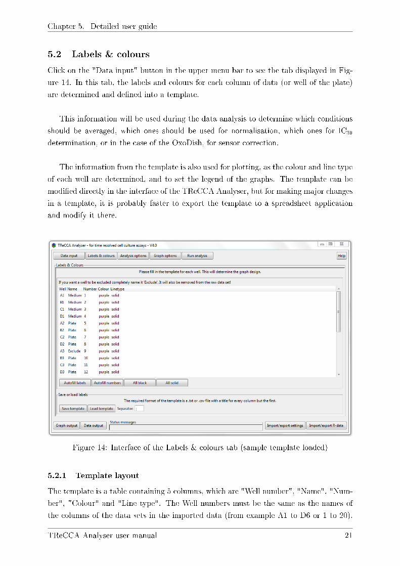
Click on the "Data input" button in the upper menu bar to see the tab displayed in Fig-
ure 14. In this tab, the labels and colours for each column of data (or well of the plate)
are determined and de�ned into a template.
This information will be used during the data analysis to determine which conditions
should be averaged, which ones should be used for normalisation, which ones for IC50
determination, or in the case of the OxoDish, for sensor correction.
The information from the template is also used for plotting, as the colour and line type
of each well are determined, and to set the legend of the graphs. The template can be
modi�ed directly in the interface of the TReCCA Analyser, but for making major changes
in a template, it is probably faster to export the template to a spreadsheet application
and modify it there.
Figure 14: Interface of the Labels & colours tab (sample template loaded)
5.2.1 Template layout
The template is a table containing 5 columns, which are "Well number", "Name", "Num-
ber", "Colour" and "Line type". The Well numbers must be the same as the names of
the columns of the data sets in the imported data (from example A1 to D6 or 1 to 20).
TReCCA Analyser user manual 21

Chapter 5. Detailed user guide
These can be detected automatically and added to the template by clicking the "Auto�ll
labels" button.
The Name can be any type of character string, but many special characters will not
be recognised or will cause problems depending on the system running. This name will
be used for the legend labels and to determine groups of wells for averaging for example.
Instead of using the "Name", it is also possible to use the "Number" column to de�ne
groups of columns/wells. The oxygen calibration pop-up also determines the groups of
wells using this number. If all the numbers in the template are the same, the legends
of the graphs will be sorted alphabetically. By assigning each condition a number, it
is possible to determine in which order each label will appear in the legend; the name
assigned the smallest number will be displayed �rst and so on. As a general rule, in the
case of the legend for average conditions, the "Number", "Colour" and "Line type" of the
�rst occurring sample of a speci�c group will be used to represent the average condition.
For example, if Well 1 has the name "Medium" and the colour "red", and Well 2 has the
name "Medium" and the colour "blue", then when representing the "Medium" average
the line will be red.
The "Colour" must be a character string referring to one of the 657 R colours. A
list of the available colours can be found online (by searching "R colours") or by typing
colours() in the R console to get the available list. The "Line type" can be "solid",
"dashed", "dotted", "dotdash", "longdash", "twodash" or "blank" (not be visible).
5.2.2 Filling the template automatically
When creating a new template, using the auto �ll options will make sure the template
has the right format. The "Auto�ll labels" button will detect all the column names in the
input data and place them in the Well column. This requires the data to be loaded already.
Make sure that all the column names are di�erent inside one imported �le. When
importing data from two separate �les, all the Well names of the second �le will be mod-
i�ed to display ".1" at their end. In this way, it is possible to import �les with identical
column names without having to change these names manually. In the case of importing
three �les which all have A1 as �rst column name, these will appear as A1, A1.1 and A1.2
in the "Well" column of the template. The "Auto�ll labels" button will automatically
�ll the Colour column with "black" and the rest of the template with "0", so this button
should be the �rst used and be sure to save the template displayed beforehand if necessary.
22 TReCCA Analyser user manual
Chapter 5. Detailed user guide
The "Auto�ll numbers" button will give a unique number to all the wells. "All black"
and "All solid" will set all the colours to black and all the line types to solid respectively.
5.2.3 Saving and loading
As mentioned before, even if it is possible to modify the template directly in the TReCCA
Analyser interface, it is probably easier to use a classical spreadsheet program for major
changes, as for example after using the auto �ll options. To save the template click the
"Save template" button and type a �le name ending with .txt or .csv. It is also possible
to type a path to a di�erent folder within the current working directory (for example,
"Templates/NewTemplate.csv"). The template can then be changed at will and loaded
again once it is completely �lled. To load a previously saved template, click on the "Load
template" button, which will open the �le chooser. When importing a template, be sure
to specify the right cell separator. After importing saved settings, the template will have
to be loaded again from the �le system for the program to run smoothly.
5.2.4 Excluding data from the analysis
In order to exclude one well from the data analysis (if you realise that it is an outlier
condition for example), it is possible to type "Exclude" as its name, thus bypassing the
more time-consuming step of actually deleting the column from the original data set and
then from the template. Naming a condition(s) "Exclude" will automatically remove the
column(s) from the data set before any analysis is run, so it will not be taken into account
for the average calculation, IC50 determination, oxygen consumption determination... In
the graphs of the raw data though, the conditions may be represented in the wrong colour
as the template is not automatically modi�ed. If it is important for the individual condi-
tions to be represented in the right colour, then it will be necessary to delete the condition
from the .csv �le and the template. Either way, it is possible to access the reduced data
set as "Raw data" after the analysis is run.
5.3 Analysis options
In the "Analysis options" tab displayed in Figure 15 the analysis to be performed on the
data are selected and the corresponding settings are �lled in. First �ll in the "Analy-
sis selection" (top part of the screen). As the boxes are ticked, new �elds to �ll in will
appear in the bottom part of the screen corresponding to each possible analysis and the
respective settings that have to be �lled in. These settings are described in the following
paragraphs and for a more precise description of the mathematical calculations that take
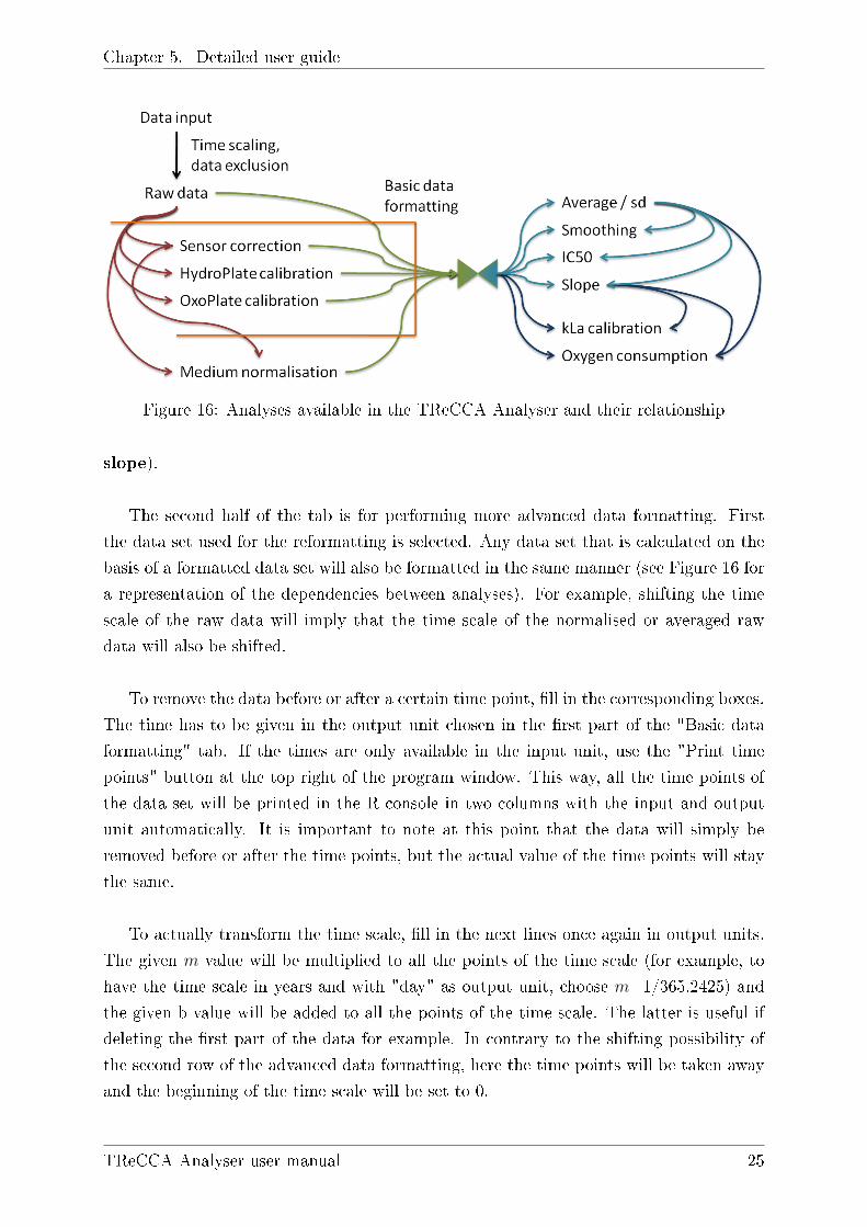
place, please refer to chapter 6 Technical details. An overview of the possible analyses
and their relations is displayed in Figure 16.
TReCCA Analyser user manual 23

Chapter 5. Detailed user guide
Figure 15: Analysis options tab with the basic data formatting option
Each analysis tab has a "Rerun xxx only" button which starts the analysis of only
the actual analysis in order to save time and prevent having to run the whole analyses
repeatedly. By pressing a "Rerun xxx only" button, a new window will appear asking if
the analysis based on this calculation should also be updated (refer to Figure 16 for an
overview of the dependencies). For example, if the normalisation target value is changed
and the "Rerun normalisation only" button is pressed, then the TReCCA Analyser will
ask whether the average normalisation calculation, which is based on the normalised data
should also be accordingly recalculated.
5.3.1 Basic data formatting
The "Basic data formatting tab" is always displayed in the "Analysis options" window,
as seen in Figure 15. The �rst half of the tab has to be �lled in accordance with the
time-resolved experiment, the second half is optional.
In the �rst row, tick the time unit of the input data. The time unit used for all the
output graphs can be chosen in the second row and the TReCCA Analyser will automati-
cally perform the corresponding unit conversions, if necessary. The output time scale unit
will also have an in�uence on the slope calculation of the data (see part 5.3.8 Numerical
24 TReCCA Analyser user manual
Chapter 5. Detailed user guide
Figure 16: Analyses available in the TReCCA Analyser and their relationship
slope).
The second half of the tab is for performing more advanced data formatting. First
the data set used for the reformatting is selected. Any data set that is calculated on the
basis of a formatted data set will also be formatted in the same manner (see Figure 16 for
a representation of the dependencies between analyses). For example, shifting the time
scale of the raw data will imply that the time scale of the normalised or averaged raw
data will also be shifted.
To remove the data before or after a certain time point, �ll in the corresponding boxes.
The time has to be given in the output unit chosen in the �rst part of the "Basic data
formatting" tab. If the times are only available in the input unit, use the "Print time
points" button at the top right of the program window. This way, all the time points of
the data set will be printed in the R console in two columns with the input and output
unit automatically. It is important to note at this point that the data will simply be
removed before or after the time points, but the actual value of the time points will stay
the same.
To actually transform the time scale, �ll in the next lines once again in output units.
The given m value will be multiplied to all the points of the time scale (for example, to
have the time scale in years and with "day" as output unit, choose m=1/365.2425) and
the given b value will be added to all the points of the time scale. The latter is useful if
deleting the �rst part of the data for example. In contrary to the shifting possibility of
the second row of the advanced data formatting, here the time points will be taken away
and the beginning of the time scale will be set to 0.
TReCCA Analyser user manual 25
Chapter 5. Detailed user guide
The last box will multiply all the data by a given number allowing a conversion of the
measurement unit. In this way, it is possible for example to convert data from milimolars
to molars by entering 1000.
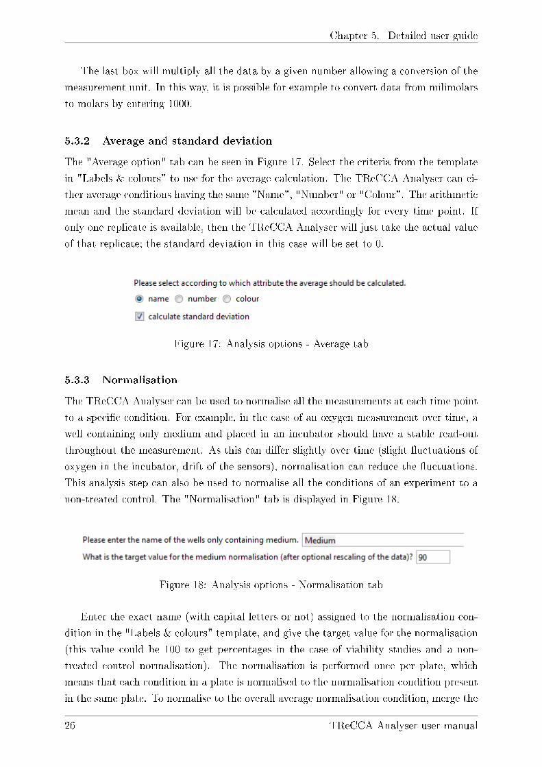
5.3.2 Average and standard deviation
The "Average option" tab can be seen in Figure 17. Select the criteria from the template
in "Labels & colours" to use for the average calculation. The TReCCA Analyser can ei-
ther average conditions having the same "Name", "Number" or "Colour". The arithmetic
mean and the standard deviation will be calculated accordingly for every time point. If
only one replicate is available, then the TReCCA Analyser will just take the actual value
of that replicate; the standard deviation in this case will be set to 0.
Figure 17: Analysis options - Average tab
5.3.3 Normalisation
The TReCCA Analyser can be used to normalise all the measurements at each time point
to a speci�c condition. For example, in the case of an oxygen measurement over time, a
well containing only medium and placed in an incubator should have a stable read-out
throughout the measurement. As this can di�er slightly over time (slight �uctuations of
oxygen in the incubator, drift of the sensors), normalisation can reduce the �uctuations.
This analysis step can also be used to normalise all the conditions of an experiment to a
non-treated control. The "Normalisation" tab is displayed in Figure 18.
Figure 18: Analysis options - Normalisation tab
Enter the exact name (with capital letters or not) assigned to the normalisation con-
dition in the "Labels & colours" template, and give the target value for the normalisation
(this value could be 100 to get percentages in the case of viability studies and a non-
treated control normalisation). The normalisation is performed once per plate, which
means that each condition in a plate is normalised to the normalisation condition present
in the same plate. To normalise to the overall average normalisation condition, merge the
26 TReCCA Analyser user manual

Chapter 5. Detailed user guide
data �rst in a spreadsheet application and import them as one �le.
5.3.4 OxoDish sensor calibration
This option is only available once "PreSens OxoDish" has been selected in the "Data
input" window in the "Data layout" part. It is displayed in Figure 19.
Figure 19: Analysis options - OxoDish sensor calibration tab
When measuring each sensor of an empty 24-well OxoDish (PreSens Precision Sens-
ing GmbH, more information is available in the SensorDishes & SensorVials instruction
manual), a read-out di�erence of between 2 and 8% can be noticed between each sensor,
although when being empty the value should be exactly the same. This slight di�erence
can be reduced thanks to the TReCCA Analyser. To do so, �rst measure the empty
sensor plate under the experimental conditions (temperature, humidity...) on the SDR
Reader that will be used later for the experiment, until the readout is stable for at least
5 time points. This will give information about the average o�set value for each well,
which can then be set to a theoretical target value (for example 100% of air saturation
if working in the lab or 95% of air saturation if working in an incubator with 5% CO2).
After the sensor calibration, all the wells will start at a much more similar value. For
more calculation details, please refer to part 6.3 OxoDish sensor calibration.
First �ll in how many time points should be used for the sensor correction (once the
read out is stable, 10 points is a good number) and enter the time point of the last of
these time points in the input unit. The TReCCA Analyser will take the value of the
time point given and for example the 9 time points before this one, to calculate the basis
for moving the whole dataset to a target starting value which must also be given. Span
and Plateau are two values which determine the exact form of the calibration curve for
each OxoDish lot. Some Span and Plateau values are presented in Table 2. As a rough
estimation it is also possible to work with the default settings.
5.3.5 OxoPlate oxygen conversion
This option is only available once "PreSens OxoPlate" has been selected in the "Data
input" window in the "Data layout" part. It is displayed in Figure 20.
TReCCA Analyser user manual 27

Chapter 5. Detailed user guide
OxoDish lot number Span PlateauOD-1437-01 2168 -201.9OD-1407-01 2062 -191.1OD-1333-01 2081 -194.5OD-1319-01 2406 -225.2OD-1309-01 2034 -187.8OD-1308-01 2026 -188.5OD-1245-01 2290 -215.0OD-1228-01 2193 -209.8OD-1220-01 2226 -208.6OD-1142-01 2123 -200.5OD-1133-01 2161 -201.6OD-1120-01 2105 -201.7OD-1107-01 2010 -187.6OD-1045-01 2079 -194.6OD-1030-01 2208 -210.0
Table 2: Span and Plateau values for di�erent SDR lots
Figure 20: Analysis options - OxoPlate oxygen conversion
When using an OxoPlate (PreSens Precision Sensing GmbH) with a classical spec-
trophotometer, the emission intensity of a luminophore that is quenched by oxygen is
measured in comparison to the emission intensity of a reference luminophore (see the
OxoPlate instruction manual on the PreSens homepage for more precise information).
The ratio of the indicator luminophore over the reference luminophore then has to be
converted by the user to actual oxygen values using two calibration solutions: one con-
taining a 100% of oxygen, Cal100, and one containing a chemical which depletes all the
oxygen present by reacting with it, Cal0. This calibration step can be done once for each
lot of OxoPlates or once for each plate and during the whole course of the experiment.
The time-resolved calibration of each plate separately leads to more precise and less noisy
results.
Whatever the calibration method, the TReCCA Analyser will convert the relative
emission intensity data automatically, and if available in a time-resolved manner, accord-
ing to the formulas described in the OxoPlate user manual. For more calculation details,
28 TReCCA Analyser user manual
Chapter 5. Detailed user guide
please refer to part 6.4 OxoPlate oxygen conversion.
First enter the exact names assigned in the template in "Label & colours" for the 0%
and 100% oxygen calibration solutions (often Cal0 and Cal100). If the lot of plates is
pre-calibrated, add two columns to the data where each one contains the Cal0 and Cal100
average value for conversion for each time point of the data. If there are several columns
with the calibration solutions, the data will be converted according to the average of
those conditions. The conversion will be done per imported plate, so for all the data to
be converted according to the overall average conditions of all the plates, merge the data
in one �le.
Select the desired oxygen unit for the output data, according to the ambient temper-
ature and pressure. If the assay conditions di�er from the given options, please choose
"other" for either of the conditions and enter the unit conversion factor manually in the
last slot. To calculate the unit conversion factor, an excel sheet is provided under "Tools
and utilities" on the PreSens homepage.
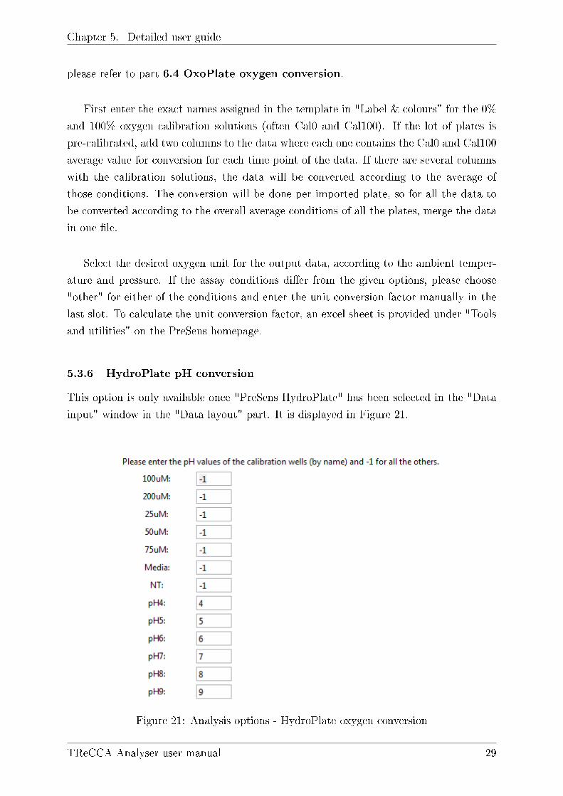
5.3.6 HydroPlate pH conversion
This option is only available once "PreSens HydroPlate" has been selected in the "Data
input" window in the "Data layout" part. It is displayed in Figure 21.
Figure 21: Analysis options - HydroPlate oxygen conversion
TReCCA Analyser user manual 29

Chapter 5. Detailed user guide
When using a HydroPlate (PreSens Precision Sensing GmbH) with a classical spec-
trophotometer, the emission intensity of a luminophore that is quenched di�erently de-
pending on the pH is measured in comparison to the emission intensity of a reference
luminophore (See the HydroPlate instruction manual on the PreSens homepage for more
precise information). The ratio of the indicator luminophore over the reference luminophore
then has to be converted by the user to actual pH values using six calibration solutions
at pH values between 4.0 and 9.0. The calibration can be done once for each lot of Hy-
droPlates or once for each plate and during the whole course of the experiment. The
time-resolved calibration of each plate separately leads to more precise and less noisy
results.
Whatever the calibration method, the TReCCA Analyser will convert the relative
emission intensity data automatically, and if available in a time-resolved manner, accord-
ing to the formulas described in the HydroPlate user manual. For more calculation details,
please refer to part 6.5 HydroPlate pH conversion.
For each name of the template that appears in the "HydroPlate conversion" tab, enter
the corresponding pH value and -1 for the wells that are irrelevant to the HydroPlate
pH conversion as seen in Figure 21. If you pre-calibrated the lot of plates, add columns
to your data where each column contains a pH relative intensity average repeated for
each time point of the data. If there are several columns with the calibration solutions,
the data will be converted according the average of those conditions.The conversion will
be done per imported plate, so for all the data to be converted according to the overall
average conditions of all the plates, merge the data in one �le.
5.3.7 Data smoothing
The TReCCA Analyser can be used to smoothen the data, which is especially necessary to
reduce the data noise before calculating the slope of the data (see part 5.3.8 Numerical
slope). For smoothing, each data point will be replaced by the average of the actual data
point and of its surrounding neighbourhood. The "Data smoothing" tab can be seen in
Figure 22.
First choose the number of points to be selected in each neighbourhood. This should
always be an odd number so as to include the actual data point and the same number
of time points on either side of the actual data point. It is important to note that the
total number of time points in each data set will be reduced after smoothing; if n is the
neighbourhood number then (n − 1)/2 time points will be missing from the beginning
and the end of the data set. Also, the bigger the neighbourhood, the smoother and less
30 TReCCA Analyser user manual

Chapter 5. Detailed user guide
Figure 22: Analysis options - Data smoothing
precise the data will get.
Select the data set(s) that should be smoothed by the TReCCA Analyser by ticking
the corresponding boxes. For more details about the formulas used for the smoothing
calculations, please refer to part 6.6 Data smoothing.
5.3.8 Numerical slope
Calculating the slope of time-resolved data can provide valuable information as it will
highlight the changes in the speed of the observed phenomenons rather than their actual
value. It is important to note that the unit of the calculated slope will be the measure-
ment unit divided by the output time unit. The y-axis label of the slope graphs will
have to be changed manually by �lling in the "Y-axis label" in the "Graph options" tab
(please refer to part 5.4 Graph options). In many cases, it can be useful to smoothen
the data before using it for slope calculation, as noise could hide the actual data trends.
The "Slope" tab can be seen in Figure 23.
Figure 23: Analysis options - Numerical slope
Fill in the number of points to be included in each neighbourhood as explained in
part 5.3.7 Data smoothing. To use non-smoothed data, �ll in the number 1. The
slope of each data point will be determined by performing a linear �t of this point and
n number of (smoothed) points on either side of it. Select the number of points to be
TReCCA Analyser user manual 31

Chapter 5. Detailed user guide
used for linear �tting, which will determine how precisely the slope should be determined
for each data point. It is important to note that the total number of time points in each
data set will be reduced after slope calculation; if n is the number of points on either
side, then n time points will be missing from the beginning and the end of the data set.
Finally, select the data set(s) for which the slope should be calculated by the TReCCA
Analyser by ticking the corresponding boxes. For more details about the formulas used
for the slope calculations, please refer to part 6.7 Numerical slope.
5.3.9 Oxygen consumption
The TReCCA Analyser will convert measured oxygen values to actual oxygen consump-
tion values, for all experimental set-ups that �t the model used. The di�usion of oxygen
into the liquid should be approximated linear, with the sensor being at the bottom of the
well and the lateral di�usion of oxygen being negligible. The calculations implemented
here are based on previous publications where the assumptions of the model are described
in more precisely 1 2 3. For more details about the formulas used for the oxygen consump-
tion, please refer to part 6.8 Oxygen consumption.
Figure 24: Analysis options - Oxygen consumption
The "Oxygen consumption" tab can be seen in Figure 24. First �ll in the oxygen
concentration of the fully saturated environment (this would typically be 100% of air sat-
uration for a measurement in the lab or 95% of air saturation for a measurement in the
incubator with 5% CO2). If this is the same value as the one used for sensor correction
(for the OxoDish users) or for medium normalisation, click the corresponding "use sensor
correction target value" and "use medium normalisation target value" buttons.
1K. Eyer, A. Oeggerli, and E. Heinzle. On-line gas analysis in animal cell cultivation: II. methods foroxygen uptake rate estimation and its application to controlled feeding of glutamine. Biotechnology andBioengineering, 45(1):54-62, 1995.
2R. Hermann, M. Lehmann, and J. Büchs. Characterization of gas-liquid mass transfer phenomenain microtiter plates. Biotechnology and Bioengineering, 81(2):178-186, 2003.
3G. John, I. Klimant, C. Wittmann, and E. Heinzle. Integrated optical sensing of dissolved oxygen inmicrotiter plates: a novel tool for microbial cultivation. Biotechnology and Bioengineering, 81(7):829-836,2003.
32 TReCCA Analyser user manual

Chapter 5. Detailed user guide
The experimental set-up �rst has to be calibrated in order to determine the di�usion
constants. This can either be done using the TReCCA Analyser (See part 5.3.10 Oxy-
gen consumption calibration of the manual) and loading a calibration �le which will
automatically �ll in the following �elds, or by �lling in the �elds manually for the oxygen
mass transfer coe�cient kLa value and error. It is essential that the time unit used for
the kLa value and for calculating the slope of the data be the same.
To change the unit of the oxygen measurement, �ll in the corresponding unit con-
version factor. To calculate the unit conversion factor, the excel sheet provided by the
company PreSens GmbH under "Tools and utilities" on the PreSens homepage can be
useful. Enter the Y-axis label that should be used for the converted oxygen consumption
and choose the data that should be used for the oxygen consumption calculation.
5.3.10 Oxygen consumption calibration
In order to convert the oxygen measurement data to actual oxygen consumption data, it is
necessary to �rst calibrate the system and determine its oxygen mass transfer coe�cient
kLa. The use of this constant is further detailed in part 5.3.9 Oxygen consumption.
Under the experimental conditions, deplete the oxygen in each well by using either
a chemical that will react with oxygen to deplete it, such as sodium dithionite Na2S2O4
or sodium sulphite Na2SO
3, or by using a nitrogen gas chamber. Note that the cited
chemicals, while being easier to use, might react with the composition of the media. Once
each well has a read-out of near to 0% oxygen, measure oxygen di�using back into the
system by either waiting for all the chemical substance to be consumed or by placing the
plate in an oxygen saturated environment again. The speed at which the oxygen rises in
each well will determine the oxygen mass transfer coe�cient kLa.
First import the calibration data into the TReCCA Analyser, �ll in the template and
perform the wanted analysis including probably averaging and de�nitely slope calcula-
tion. It is important to run a slope calculation as the data will be needed for the oxygen
consumption calibration.
To reach the calibrating platform, click on the button "Calibrate oxygen consump-
tion" at the top right of the "Analysis options" tab. The TReCCA Analyser will ask
for con�rmation that the slope calculation has been done, as seen in Figure 25, and once
"Continue with the calibration" is clicked a new pop-up window will appear, as seen in
Figure 26.
TReCCA Analyser user manual 33

Chapter 5. Detailed user guide
Figure 25: Pop-up before oxygen calibration
First �ll in the data that should be used for the oxygen calibration. Then decide
which part of the curves are linear and should be used for the calibration by �lling in the
corresponding time-frame and Y-axis limits of the data. Indicate the value of the oxygen
in the fully saturated environment. The names that appear in this section are determined
by the numbers chosen in the "Labels & colours" window under the columns "Number"
of the template. Each condition that has the same number will be analysed together and
plotted under the same chosen name entered in the following boxes.
Figure 26: Oxygen calibration window - Data preview
The "Refresh data preview" button refreshes the visualisation of the selected calibra-
tion area chosen that is delimited by four red lines. Once everything is set, press the "Run
34 TReCCA Analyser user manual

Chapter 5. Detailed user guide
calibration" button. Two new tabs will appear next to the "Data preview": "Resulting
values" and "Plot result", as seen in Figures 27 and 28 respectively. In the last tab, the
di�usion �ux, d[O2]/dt is depicted against the oxygen level. The line that �ts this data
has a slope that is equal to -kLa. The numerical value of the kLa for each condition, as well
as the standard error and the R squared of the linear �t are presented in the "resulting
values" tab.
The calibration data can be saved by pressing the "Save calibration" button. This �le
cannot be opened by traditional spreadsheet applications but can be loaded directly into
the TReCCA Analyser as described in part 5.3.9 Oxygen consumption. By clicking
the "Save plot" button, the displayed graph will be saved in the folder currently being
used for saving.
5.3.11 IC50 determination
The TReCCA Analyser can calculate the IC50 or EC50 of a drug automatically and in a
time-resolved manner, thanks to the IC50 tab displayed in Figures 29 and 30.
First select the data set that should be used for the IC50 calculation, as seen in Fig-
ure 29. Then, choose the time points, in the input unit, between which the IC50 should
be calculated. For the log-logistic �t of the data to be possible at every time point, it
is important to select the time frame where the conditions are su�ciently di�erent from
each other. If the data cannot be �tted at one time point, then all the IC50 �ts will not
appear in the graph output. It is then necessary to change the selected time points.
In order to speed up the analysis time of the data, it is possible to calculate the IC50
for only some of the data, for example for every third time point. Fill in the frequency of
the calculation accordingly.
Select which function to use to �t the data. For IC50 determination, the 4 parameter
log-logistic curve is the most commonly used. An exact description of each �tting for-
mula can be found in 6.10 IC50 determination. Enter the X-axis label that should be
displayed in the IC50 graphs.
Finally, enter the concentration of each condition used for IC50 determination without
any unit in front of the corresponding condition. The wells that are irrelevant to the IC50
determination should be �lled in with -1, as seen in Figure 30.
TReCCA Analyser user manual 35

Chapter 5. Detailed user guide
Figure 27: Oxygen calibration window - Resulting values
Figure 28: Oxygen calibration window - Plot result
36 TReCCA Analyser user manual

Chapter 5. Detailed user guide
Figure 29: Analysis options - First part of the IC50 tab
Figure 30: Analysis options - Second part of the IC50 tab
5.4 Graph options
In the "Graph options" tab, as seen in Figure 31, �ll in the settings to determine the
appearance of the graphs. All the options that are �lled in this part can be changed after
the graphs are visible. Many other settings can be modi�ed after the analysis is run in
the "Graph output" tab.
5.4.1 General
In the top part of the window, choose if the graphs should have titles and subtitles and
if so, what these titles should be. The title will be displayed in the exact same form
TReCCA Analyser user manual 37

Chapter 5. Detailed user guide
Figure 31: Graph options tab
above every single graph. The subtitles are displayed between the title and the plot on
the corresponding graph.
5.4.2 Axes
Choose the label and limits of each axis. To display limits optimised by the program,
choose 10 000 as minimum and maximum limit. These settings will be applied to all the
graphs unless mentioned otherwise in the speci�c "Analysis options" tab.
5.5 Run analysis
Once all the settings are set in the "Data input", "Labels & colours", "Analysis options"
and "Graph options" tabs, click on the "Run analysis" button. All the settings, imported
data and the template are checked for validity.
A pop-up window will appear asking the name of the results folder to be created,
as seen in Figure 32. This folder will automatically be created in the current working
directory and within this folder the current settings are also saved automatically. It is
possible to enter a path leading inside di�erent folders included in the working directory
as long as the upper directories are already created.
38 TReCCA Analyser user manual

Chapter 5. Detailed user guide
Figure 32: Pop-up window to run the analysis
If this pop-up window does not show up, then another pop-up window with a sugges-
tion about what has to be corrected will probably appear. If this is not the case, make
sure all the "Status messages" at the bottom middle of the program are clear and check
the error messages in the R console. In extreme cases, restarting the program can also be
an option.
After the name of the result folder is given, the analysis will start running. This will
take a di�erent amount of time depending on the size of the data sets, the variety and
complexity of the analyses that have to be performed and the speed of the computer that
is running. As a rough estimate, most basic analyses are usually run in under a minute
and even in extreme cases, the analysis should not last more than 15 minutes.
Each time an analysis step is completed it will appear in the analysis window followed
by "done", as seen in Figure 33 and the �rst ten rows of each data set will be printed
in the R console. Under Windows the messages and data sets will appear progressively
as the analysis is performed, under Mac all the information will appear at once as soon
as all the analysis steps are �nished. Once the program has �nished running, press the
"Close" button and the raw data graph in the "Graph output" tab should be visible.
5.5.1 Graph output
After running the analysis, the "Graph output" tab should be opened automatically as
seen in Figure 34. In this tab it is possible to customise many more items on the graphs
and export them by using the buttons and drop-down menu at the bottom of the screen.
To the right, the di�erent buttons select which calculated data sets are displayed in the
graphical area. To the left, a list of checkboxes are visible which select which lines are
displayed on the graphs.
TReCCA Analyser user manual 39

Chapter 5. Detailed user guide
Figure 33: Window seen while the analysis is running
Figure 34: Graph output tab
To change options that were set previously in the "Graph options" tab, change them
40 TReCCA Analyser user manual

Chapter 5. Detailed user guide
in the corresponding tab and then press the "Refresh options" button for the changes to
be applied. To change colours, line types or names, change the template without running
the analysis again, as long as the changes do not in�uence the calculations (many of the
analysis options use the names or numbers in the template as a basis for calculation, see
the corresponding analysis details).
Graph customisation
The drop-down menu at the bottom of the screen allows the customisation of di�erent
graphical parameters. Select the parameter to be modi�ed and then use the scroll bar or
the second drop-down menu that appears to modify it. The graphs will only be modi�ed
once the slider is set, and it is also possible to click on the bar directly to skip through
bigger steps instead of pulling the slider. The di�erent possible customisations are as
follows.
- Point size: Changes the point size of all the text on the graphs (title, subtitle,
label descriptions, legend) ranging from 5.0 to 25.0.
- Legend columns: Number of columns used to display the legend (if appropriate)
ranging from 1 to 10.
- Legend position: Determines the presence of a legend or not and its position. The
possible options are: no legend, below the plot area, to the right of the plot area,
top left, top middle, top right, middle right, bottom right, bottom middle, bottom
left, middle left.
- Line width: Sets the width of the lines on the graph (grid lines and frame included)
ranging from 0.5 to 4.0.
- Grid colour intensity: Picks the intensity of the colour of the grid in percentage,
so ranging from 0 (no grid) to 100 (dark grey grid).
- Error colour intensity: For the graphs where the standard deviation is calculated
(average graphs, slope calculation and time-resolved IC50), changes the intensity of
the error display in percentage, so ranging from 0 (no error) to 100 (black error).
- White space: Varies the amount of white space around the graph and how compact
the representation is, ranging from 0.00 to 1.00. This option is present so that the
exported graphs can be used directly for power point presentations as well as for
graphs that are part of a �gure in a publication.
Line selection
The line selection determines which lines are displayed on the graph. When selecting the
lines to be displayed (also for the select all/none buttons) click the "Refresh lines" button
to show the selected lines on the actual graph.
TReCCA Analyser user manual 41
Chapter 5. Detailed user guide
Graph selection
The buttons on the right of the screen determine which graph is represented in the plot
area. Only graphs of the analyses that have been run can be represented. In the case
of the average graphs where the standard deviation was calculated, an extra tick box
appears next to the graph customisation drop-down menu. Selecting it will display the
standard deviations of the averages of the curves as a grey shade behind the averaged
line. For the slope calculation, the standard deviation tick box is also present and enables
showing the error of the linear �t on the graphs. For the time-resolved IC50
data, the
error of the �t can also be displayed. In the case of the display of the sigmoidal �ts for
the IC50
calculation, extra tick boxes appear above the customisation drop-down menu,
allowing for a further customisation of the graphs. The �rst line allows to di�erentiate
IC50�ttings by varying:
- Colour: Each �t is displayed in a di�erent colour, the concentration points are
represented as empty coloured circles.
- Line type/symbols: All the lines and symbols are black, the line types and sym-
bols vary from time-point to time-point.
- Nothing: All the lines and symbols are black, the lines are all "solid" and the
symbols are all represented as empty circles.
Exporting graphs
To export graphs, click on the "Export displayed graph" button, at the bottom right of
the plot area, and give the �le name and size of the desired output (size in inches). The
choice of the size of the �le will not in�uence the size of the text on the graph, so make
sure that the text on the graphs still �ts properly after export. To change the output
�le type, change the ending to either .pdf (Portable Document Format), .ps (PostScript
format), .svg (Scalable Vector Graphics) or .png (Portable Network Graphics). The �les
will automatically be saved to the folder speci�ed when running the analysis, included in
the working directory.
5.5.2 Data output
The "Data output" tab on the bottom of the screen contains one line for every data set
that was created during the analysis as seen in Figure 35. First �ll in the appropriate
column separator and decimal separator. Then select which data sets to export by click-
ing the corresponding tick boxes and give them �le names ending with .csv. Click the
"Export Files" button at the bottom right of the screen and the �les will all be written
into the speci�ed result folder. A pop-up window will con�rm the success of the export.
42 TReCCA Analyser user manual

Chapter 5. Detailed user guide
Figure 35: Data output tab
5.5.3 Import/export settings
In order to make it easier to rerun the analysis, it is possible to save all the settings
chosen in the program. Click on the "Import/export settings" button at the bottom right
of the screen and the pop-up window displayed in Figure 36 should appear. The �le
will be saved in the working directory. Type a �le name ending with .txt (for example
"Settings_Experiment1.txt") or a path included in the working directory followed by the
�le name (for example "ResultsA/Settings_Experiment1.txt"). These settings will also
be saved automatically when you click the "Run analysis" button under the name "au-
tosave_settings.txt".
The "Import/export settings" button, can also be used to load previously saved set-
tings by clicking the "Load" button and selecting the settings �le. The layout of the
program will then be changed accordingly. Even after importing the saved settings it will
be necessary to load the data and the template again for the analysis to run.
It is possible to customise the default settings of the TReCCA Analyser, once it is
�rst opened. To do this, set all the settings as wished and then save them using the "Im-
port/Export settings" button under the name "default_settings.txt", thereby replacing
the existing �le. The next time the TReCCA Analyser is opened, the settings should be
the way they were last left.
TReCCA Analyser user manual 43

Chapter 5. Detailed user guide
Figure 36: Pop-up for saving / loading settings.
5.5.4 Import/export R-data
To save all the data that has been imported and analysed, in order to possibly replot
graphs without rerunning the analysis for example, press the "Import/export R-data"
button. The corresponding �le should end with ".RData" and will be saved in the work-
ing directory, as described by the pop-up window.
To load previously saved R-Data, click on the "Load" button and select the correct
�le. The analysed data sets will once more be available in the R-console and for plotting.
44 TReCCA Analyser user manual

6 Technical details
In this section more details concerning the mathematical analysis of the data are pre-
sented, sorted for each analysis option available in the tab "Analysis options". For more
precise information, the actual code of the program is freely available.
6.1 Average and standard deviation
The average and standard deviation are calculated according to standard statistical formu-
las, using the prede�ned functions of R. The function for the average is mean(numerical
vector) (see Equation 6.1), where n is the number of averaged points and xi the ini-
tial value of the replicate i. The function for the standard deviation is sd(numerical
vector) and calculates the sample standard variation (see Equation 6.2), where x̄ is the
average for each time point.
mean (~x) =1
n
n∑i=1
xi (6.1)
sd (~x) =
√√√√ 1
n− 1
n∑i=1
(xi − x̄)2 (6.2)
6.2 Normalisation
The normalisation �rst calculates the average mt of all normalisation wells on one plate at
each time point (see Equation 6.1). Every data point from this plate is then normalised
according to Equation 6.3, where M is the target value for the normalisation wells, xt the
initial value for each time point and yt the value after normalisation for each time point.
yt =xt ·Mmt
(6.3)
6.3 OxoDish sensor calibration
The OxoDish sensor calibration can be divided into two distinct steps. First, all the sen-
sor read-outs inside one plate are brought to a common value, and in a second step the
sensor read-outs are homogenised from plate to plate.
45

Chapter 6. Technical details
6.3.1 Step 1: Homogenising the sensor read-outs of each plate
The �rst part of the sensor correction corrects each sensor read-out from an OxoDish (so
usually 24 independent read-outs) using an empty well sensor read-out from the beginning
of the measurement as reference (also usually 24 reference read-outs).
The calibration curve for the conversion of the phase to the oxygen level is a com-
plex equation (which is the property of PreSens Precision Sensing GmbH), which can be
modelled by the exponential Equation 6.4 quite accurately, where P is the Plateau of the
model and S the Span. The values of P and S vary from lot to lot as presented in Table 2
(see part 5.3.4 OxoDish sensor calibration).
x = P + S · ez (6.4)
In order to make the calibration curve linear and thereby allow a correction by mul-
tiplication and division, all the data is �rst converted to logarithmic values as described
in Equation 6.5.
z = ln
(x− P
S
)(6.5)
Then, instead of using a discrete point as empty well reference value, all the values for
each sensor included in a certain time frame are averaged and taken into account. This
time frame is chosen by the user and ranges from the time points t1 to tn, where tn is the
last time point at the end of the sensor calibration and n the number of points averaged
for calibration. The mean read-out over the time frame of each sensor s is then described
by Equation 6.6.
ms =1
n
n−1∑i=0
zt1+i,s (6.6)
The mean read-out value for the total plate mp is determined by averaging the average
read-outs ms for each sensor, as described in Equation 6.7, where wp is the number of
wells per plate.
mp =1
wp
wp∑j=1
mj (6.7)
The corrected values x̃ are then calculated according to Equation 6.8, whereby the
data, which is still in a logarithmic scale, is then also reconverted back to the actual data
values through the exponential function.
x̃t,s = P + S · empms
·zt,w (6.8)
46 TReCCA Analyser user manual

Chapter 6. Technical details
6.3.2 Step 2: Setting the average read-out to a de�ned target
In a second step, the corrected values x̃ are linearly normalised to a target value T chosen
by the user according to the experimental conditions. The read outs of the correction
time frame for each sensor mc,s are averaged according to the Equation 6.9.
mc,s =1
n
n−1∑i=0
x̃t1+i,s (6.9)
The resulting corrected oxygen values at the time point t and for the sensor s are then
yt,s (Equation 6.10).
yt,s =x̃t,s · Tmc,s
(6.10)
6.4 OxoPlate oxygen conversion
Prior to the data processing by the TReCCA Analyser, the user has to divide the intensity
measurement of the indicator luminophore by that of the reference measurement for each
time point in a classical spreadsheet application. The resulting data (called IR) can then
be loaded to the TReCCA Analyser to be converted to oxygen values.
The OxoPlate oxygen conversion is performed per plate using the two calibration
conditions that expose the sensors to 0% and 100% oxygen in percentage of air saturation.
The TReCCA Analyser �rst calculates the average of all 0% and 100% oxygen wells for
each time point (again using Equation 6.1), thereby determining the values over time of k0t
or k100t respectively. Every data point is then converted according to the Equation 6.11,
where F is the unit conversion factor and xt the value IR over time.
yt = F · 100 ·k0txt
− 1k0t
k100t− 1
(6.11)
6.5 HydroPlate pH conversion
Just as in the case of the OxoPlate, prior to the data processing by the TReCCA Analyser,
the user has to divide the intensity measurement of the indicator luminophore by that of
the reference measurement for each time point in a classical spreadsheet application. The
resulting data (called IR) can then be loaded to the TReCCA Analyser to be converted
to pH values.
The HydroPlate pH conversion is performed per plate using 6 calibration conditions
that expose the sensors to di�erent pH conditions covering the range of pH 4.0 to pH 9.0.
The TReCCA Analyser �rst calculates the average of the calibration pH wells for each
time point (again using Equation 6.1). These values are �tted using a four parameter
TReCCA Analyser user manual 47

Chapter 6. Technical details
logistic function curve over time (the function L4 of the drc package), as described in
Equation 6.12.
f(x) = c+d− c
1 + exp (b (log (x) − log (e)))(6.12)
From this �t, the calibration constants Imin = d, Imax = c, dpH = 1/b, pH0 = log(e)
are determined. Every data point is then converted according to the Equation 6.13, where
xt is the value IR over time.
yt = ln(Imin,t − Imax,t
xt − Imax,t
− 1) · dpHt + pH0,t (6.13)
6.6 Data smoothing
The data smoothing uses the built in mean function, but in this case an average of several
points over time is calculated in order to reduce �uctuations according to the formula
given in Equation 6.14, where n is the number of time points to average. Every time
point is thereby replaced by the average of the time point and (n − 1)/2 neighbours on
either side. This causes the loss of (n− 1)/2 data points in the beginning and the end of
the measurement, as these points do not have the necessary neighbours.
yt =1
n
t+n−12∑
i=t−n−12
xt (6.14)
6.7 Numerical slope
For the numerical slope calculation, it is usually necessary to smoothen the data �rst to
get rid of the noise. The TReCCA Analyser always uses a smoothed data set for the
calculation, but the number of points used or the smoothing can be set to 1 in which case
no smoothing will actually occur. For the slope calculation, a certain number of points n
on either side of the currently processed time point x are used for a linear model �t (as
described by Equation 6.15). The linear model �t is a built in function of R and yields
the slope m and the corresponding residual ε which is displayed as the standard deviation
on the graphs.
(yx−n, · · · , yx+n) = m · (tx−n, · · · , tx+n) + c (6.15)
6.8 Oxygen consumption
As already described in the part 5.3.9 Oxygen consumption, the calculations imple-
mented in this part of the TReCCA Analyser are based on previous publications (Eyer et
al., 1995; Hermann et al., 2003; John et al., 2003) and can only be used if the experimental
conditions �t the prerequisites of the model described in these publications. For example,
in our experimental set-ups using 96-well plates, this is the case if the solutions are mixed
48 TReCCA Analyser user manual

Chapter 6. Technical details
over time, but not the case if they are not shaken. The �rst step in knowing if the model
applies or not is to see whether for at least certain oxygen saturation values, the oxygen
saturation value is proportional to the rate of change of the oxygen saturation value when
the oxygen consumption rate is 0. This is described in more detail in parts 5.3.10 Oxy-
gen consumption calibration and 6.9 Oxygen consumption calibration.
When the model applies, the oxygen uptake rate (OUR) is then described by the
Equation 6.16, where [O2] is the measured oxygen concentration, [O∗2] the concentration
of the saturated liquid phase and kLa is the oxygen mass transfer coe�cient. For the
OUR to be correct, it is essential that the kLa and the d[O2]/dt have the same time unit.
OUR = kLa ([O∗2] − [O2]) −
d [O2]
dt(6.16)
6.9 Oxygen consumption calibration
The calculations implemented in the TReCCA Analyser are based on the assumption that
the general formula of the oxygen balance is as described in Equation 6.17, where [O2] is
the measured oxygen concentration, [O∗2] the concentration of the saturated liquid phase
and kLa is the oxygen mass transfer coe�cient. The change in oxygen over time is equal
to the di�usion of oxygen into the well minus the amount of oxygen consumed by the
cells, yeast, bacteria or chemical reaction.
d [O2]
dt= kLa ([O∗
2] − [O2]) −OUR (6.17)
To perform the oxygen consumption calibration, it is necessary to work under condi-
tions where the OUR = 0, which means by working with wells without any cells, yeast,
bacteria, enzymes, etc. Equation 6.17 can then be simpli�ed to Equation 6.18, where
kLa[O∗2] is a constant.
d [O2]
dt= kLa[O∗
2] − kLa [O2] (6.18)
The oxygen concentration [O2] is set to 0 by using either nitrogen or chemicals that react
with oxygen, as described in part 5.3.10 Oxygen consumption calibration, and then
the di�usion of oxygen back into the solutions is measured over time until it reaches the
level of the ambient saturation.
The rate of oxygen change over time d[O2]/dt can be calculated using the slope function
of the TReCCA Analyser. Plotting this slope against the actual oxygen value [O2] and
�tting a linear model then yields kLa and the corresponding residual ε for the �t. Using
the plots that are displayed in the oxygen consumption calibration interface (Figure 26, 27
TReCCA Analyser user manual 49

Chapter 6. Technical details
and 28) it is possible to determine if the model for the oxygen balance in the experimental
set-up is valid and if so, to set the range for the linear �t in order to exclude the initial
or �nal phases of the measurement.
6.10 IC50 determination
For the IC50 calculation the TReCCA Analyser uses concentrations assigned to the labels
of the data by the user. It is also possible to select how many time points to skip in
order to reduce the run time of the calculation. From this a data set is created, where
the concentrations replace the well names, fewer time points are included, and those wells
which do not belong to the IC50 calculation are excluded. The IC50 is calculated for
each line of the data set, which represents one time point. The possible models used
for determining the IC50 are included in the drc package and are the two-, three-, four-
and �ve-parameter log-logistic models as depicted in Equations 6.19, 6.20, 6.21, 6.22
respectively. The error is reduced by a non-linear least-squares method.
f(x) =1
1 + exp (b (log (x) − log (e)))(6.19)
f(x) =d
1 + exp (b (log (x) − log (e)))(6.20)
f(x) = c+d− c
1 + exp (b (log (x) − log (e)))(6.21)
f(x) = c+d− c
(1 + exp (b (log (x) − log (e))))f(6.22)
The curve of the IC50 �t for each time point, as well as a curve of the IC50 value over
time are shown.
50 TReCCA Analyser user manual

7 Trouble shooting
This section is designed to help �nd a fast solution to any error message or problem that
may be encountered while using the TReCCA Analyser.
7.1 Error messages
Error messages regarding the settings are shown in the status messages bar in the bottom
of the program window. This bar is a scrollable list. In Table 3 all possible error mes-
sages are listed in alphabetical order. A short explanation and solution to each message
is presented and each error message is linked to the section in the manual it is related to
for more details. Errors that prevent an action from being taken will appear as a pop-up
window. The Tables 4, 5, 6 and 7 give suggestions to solve each problem.
7.2 R console
Some error messages and warnings can appear in the R console and be ignored. If after
solving all the error messages in the scrollable list status messages bar and all the pop-up
errors, something still is not functioning correctly, double check whether the data is cut
properly, whether there is non numerical data left in the data set (this can be checked eas-
ily using the program), whether the template contains exotic characters that might a�ect
plotting and whether all the paths and folders given are valid. If the problem persists, it
is possible to check the R console for additional complications. Many problems can then
be resolved by following the instructions in the R console, by searching the error message
on-line or by asking the questions on an online forum.
51

Chapter 7. Trouble shooting
Error message Chapter Solution
Entered path doesn't
lead to an existing �le!
Labels &
colours
Use the �le chooser properly to select the template.
If this error occurs when starting the program, the
default template from the Sample Project folder
is missing. This is �ne but the error will always
occur upon start up.
Entered paths don't
lead to existing �les!Data input
Use the button showing a folder to open a �le
chooser dialogue and select the data (typing the
�le name/path can lead to typing errors), avoiding
exotic characters in the pathways. When import-
ing Settings, make sure the input data is still in
the same place on the computer.
Given last value for
sensor calibration
can't be found in
imported data!
OxoDish
sensor
calibration
Make sure the time point is included in the data
�le. A rough time point is not enough - the exact
time point has to be given in the input unit.
Given name for nor-
malisation is not in
the labels list!
Normalisation
The name for the normalisation condition has to
be in the "Labels & colours" template in exactly
the same spelling and capital/small letter combi-
nation.
Given name for 0 %
oxygen wells is not in
the labels list!
OxoPlate
oxygen
conversion
The name has to be in the "Labels & colours"
template in exactly the same spelling and capi-
tal/small letter combination.
Given name for 100 %
oxygen wells is not in
the labels list!
OxoPlate
oxygen
conversion
The name has to be in the "Labels & colours"
template in exactly the same spelling and capi-
tal/small letter combination.
Max. number of
plates is 10!Data input
The number of plates has to be a whole number
between 1 and 10 (included).
Please enter a number
for end of IC50 calcu-
lation!
IC50 determi-
nation
Make sure the exact time point for the end of the
calculation interval given in the input unit is in-
cluded in the data �le.
Please enter a number
for normalisation tar-
get!
NormalisationEnter a target value for normalisation without any
measurement unit and . as a decimal separator.
Please enter a number
for Plateau!
OxoDish
sensor
calibration
Enter a number with . as decimal separator.
52 TReCCA Analyser user manual

Chapter 7. Trouble shooting
Please enter a number
for sensor calibration
target!
OxoDish
sensor
calibration
Enter a number with . as decimal separator.
Please enter a number
for Span!
OxoDish
sensor
calibration
Enter a number with . as decimal separator.
Please enter a number
for start of IC50 calcu-
lation!
IC50 determi-
nation
Make sure the exact time point for the start of
the calculation interval given in the input unit is
included in the data �le.
Please enter a number
for the error of the kLa
value!
Oxygen
consumptionEnter a number with . as decimal separator.
Please enter a number
for the kLa value!
Oxygen
consumptionEnter a number with . as decimal separator.
Please enter a number
for the saturated oxy-
gen concentration!
Oxygen
consumptionEnter a number with . as decimal separator.
Please enter a num-
ber for the slope �t-
ting points!
Numerical
slopeEnter a whole number superior or equal 1.
Please enter a num-
ber for the unit con-
version factor used for
the oxygen consump-
tion!
Oxygen
consumption
Enter a number with . as decimal separator. 1 for
no conversion.
Please enter a number
for the unit conversion
factor!
OxoPlate
oxygen
conversion
Enter a number with . as decimal separator for
the unit conversion of the luminescence data to
the target unit.
Please enter an odd
number for the curve
smoothing!
Data
smoothingEnter a whole odd number superior or equal to 1.
Please enter a number
> 1 for sensor calibra-
tion range!
OxoDish
sensor
calibration
Enter a number of time points for sensor correction
superior to 1 (the last time point is included and
one point is insu�cient for the correction).
Please enter a positive
number for Header
length!
Data input
If you do not have a header in your �le(s) select
"No" so the number will be ignored. Otherwise
enter a positive whole number.
TReCCA Analyser user manual 53

Chapter 7. Trouble shooting
Please enter a positive
number for last cali-
bration value!
OxoDish
sensor
calibration
The time point speci�ed for the last calibration
point must be a positive number found in the time
column of the data set (in the input unit).
Please enter a positive
number for number of
plates!
Data inputThe number of plates has to be a whole number
between 1 and 10 (included).
Please enter a posi-
tive number for skip-
ping points in IC50 cal-
culation!
IC50 determi-
nation
Enter a whole positive number for the frequency
of IC50 calculation. For all time points to be taken
into account choose 1.
Please enter numbers
for X-axis limits!
Graph
options
Enter any number with . as decimal separator and
10 000 if for automatic axis limits.
Please enter numbers
for Y-axis limits!
Graph
options
Enter any number with . as decimal separator and
10 000 if for automatic axis limits.
Please enter numerical
values > 0 or -1 only
for the IC50 doses!
IC50 determi-
nation
Enter the concentrations as positive numbers with
. as a decimal separator or -1 to exclude a condi-
tion from the IC50 calculation.
Please enter numerical
values > 0 or -1 only
for the pH values!
HydroPlate
pH
conversion
Enter the pH values as positive numbers with . as
a decimal separator or -1 to exclude a condition
from the pH conversion.
Please enter positive
numbers for wells!Data input
There has to be a positive whole number in every
�eld next to the rows for each imported plate. For
several plates, just one number in the �rst �eld is
not enough!
Please enter positive
numbers or 0 for spare
columns!
Data inputEnter a positive whole number for the data for-
matting or 0 to not delete any columns.
Please enter positive
numbers or 0 for spare
rows!
Data inputEnter a positive whole number for the data for-
matting or 0 to not delete any rows.
Please enter proper
�lenames for all the
data sets to be ex-
ported!
Data outputEnter �le names for all the chosen �les to be ex-
ported. They should all end with ".csv".
Please only enter
numerical values
for the formatting
parameters!
Basic data
formatting
Enter numbers with . as decimal separator in the
output unit for each formatting parameter.
54 TReCCA Analyser user manual

Chapter 7. Trouble shooting
Starting time point of
IC50 calculation has to
be before end point!
IC50 determi-
nation
The IC50 calculation interval time points (in input
unit) are not in the right order.
The given time point
for end of IC50 calcula-
tion can't be found in
imported data!
IC50 determi-
nation
Make sure the exact time point for the end of the
calculation interval given in the input unit is in-
cluded in the data �le.
The given time point
for start of IC50 calcu-
lation can't be found
in imported data!
IC50 determi-
nation
Make sure the exact time point for the start of
the calculation interval given in the input unit is
included in the data �le.
There are not as many
time points for cali-
bration as you want to
include!
OxoDish
sensor
calibration
There are not enough time points prior to the
starting point speci�ed. Enter a smaller number
of time points or set a higher starting time point.
You are about to re-
move the stop time
point of the sensor
correction!
Basic data
formatting
By proceeding with this basic data formatting
step, the time-point used for OxoDish sensor cali-
bration will be removed.
Your imported data
doesn't contain
enough time points
for smoothing!
Data
smoothing
Reduce the number of points set for smoothing or
prepare a data set with more time points.
Your imported data
doesn't contain
enough time points
for the slope calcula-
tion!
Numerical
slope
Reduce the number of points set for the slope cal-
culation or prepare a data set with more time
points.
Table 3: Error messages shown in the status messages bar in alphabetical order
TReCCA Analyser user manual 55

Chapter 7. Trouble shooting
General errors
The script for the TReCCA Analyser that
you are using has been modi�ed. Download
the original �les again to work with the cor-
rect version.
Error upon data import or when trying to
run the analysis. Some of the settings are in-
valid and there are errors in the status mes-
sages bar. Please look up solutions in Ta-
ble 3.
Table 4: Pop-up errors and solutions: General errors
Data input
Error upon trying to automatically �ll the
template's well number column or trying to
run the analysis. Either the data is not im-
ported yet or a severe error message occurred
upon trying to import it. The data input
is also cleared whenever settings are loaded.
Please go to the data input interface and
press import data and if necessary solve the
other error messages.
Error upon trying to import data without
getting rid of non numerical data. Your data
contains non numerical data. Either change
your tick for the data cleaning or clean the
data manually.
Error upon trying to import data from sev-
eral plates. This means that the time
columns in your �les are not identical. This
can be due to di�erent line numbers in the
�les. Otherwise it is recommended to analyse
the plates independently.
56 TReCCA Analyser user manual

Chapter 7. Trouble shooting
Error upon trying to import data. The sum
of the well numbers you speci�ed + 1 for the
time column doesn't match with the total
number of columns in the (merged) data you
tried to import. Please check the columns
again and change the numbers accordingly.
Warning pop-up that all the data that is not
recognised by the program as a number will
be replaced by 0. This will not a�ect your
original data �les.
Information pop-up. The �les imported con-
tained data that was all recognised as numer-
ical, no data point was replaced by 0.
5 discrete value(s) are not recognised as nu-
merical. Accept that they will have the value
0 or check out the original �les and modify
them. The �les could contain text such as
"Error", "> 9.0 pH" or numbers with the
wrong decimal separator.
2 whole column(s) are not recognised as nu-
merical. Accept that they will have the value
0 or check out the original �les and mod-
ify them. The columns could contain values
recognised as text such as "Error", "> 9.0
pH" or numbers with the wrong decimal sep-
arator.
TReCCA Analyser user manual 57
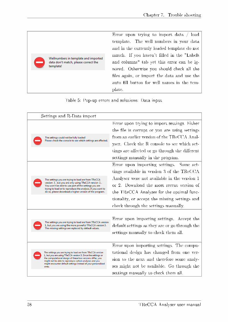
Chapter 7. Trouble shooting
Error upon trying to import data / load
template. The well numbers in your data
and in the currently loaded template do not
match. If you haven't �lled in the "Labels
and columns" tab yet this error can be ig-
nored. Otherwise you should check all the
�les again, or import the data and use the
auto �ll button for well names in the tem-
plate.
Table 5: Pop-up errors and solutions: Data input
Settings and R-Data import
Error upon trying to import settings. Either
the �le is corrupt or you are using settings
from an earlier version of the TReCCA Anal-
yser. Check the R console to see which set-
tings are a�ected or go through the di�erent
settings manually in the program.
Error upon importing settings. Some set-
tings available in version 3 of the TReCCA
Analyser were not available in the version 1
or 2. Download the most recent version of
the TReCCA Analyser for the optimal func-
tionality, or accept the missing settings and
check through the settings manually.
Error upon importing settings. Accept the
default settings as they are or go through the
settings manually to check them all.
Error upon importing settings. The compu-
tational design has changed from one ver-
sion to the next and therefore some analy-
ses might not be available. Go through the
settings manually to check them all.
58 TReCCA Analyser user manual
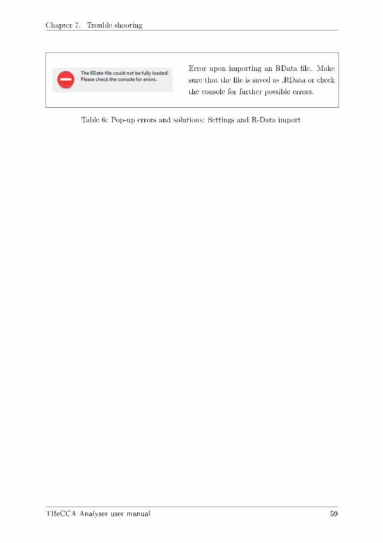
Chapter 7. Trouble shooting
Error upon importing an RData �le. Make
sure that the �le is saved as .RData or check
the console for further possible errors.
Table 6: Pop-up errors and solutions: Settings and R-Data import
TReCCA Analyser user manual 59

Chapter 7. Trouble shooting
Labels and Colours errors
Error upon trying to run the analysis. A
proper "Labels & colours" template is not
loaded yet, or has been cleared by loading
settings. Please go to the "Labels & colours"
tab and click the load template button to
open a �le chooser dialogue or create a new
template using the auto�ll buttons.
Error upon trying to import data. The
names of the columns are not unique. This
can happen easily by merging the data man-
ually. Please change the names accordingly
or use the automated �le merging to prevent
this error.
There are colours in the template which are
not recognised by the program. Please only
use colour names (and not numbers), check
there are no white spaces after the colour
name or spelling mistakes. All the valid
colours can be found by typing "colours()"
in the R console.
Error upon trying to load a template. This
means that the �rst row in the template does
not contain the right names. It might help to
remove all the quotation marks from the csv-
�le. Another reason might be the separator
chosen for loading the template.
Table 7: Pop-up errors and solutions: Labels and Colours
Graph output
Error upon visualising data after using the
"rerun" button for the data analysis. Data
sets used to calculate the data shown on this
graph have been modi�ed a posteriori.
Table 8: Pop-up errors and solutions: Graph output
60 TReCCA Analyser user manual

List of Figures
1 R Console just after launch on Windows . . . . . . . . . . . . . . . . . . . 9
2 R Console just after launch on Mac . . . . . . . . . . . . . . . . . . . . . . 10
3 Package installation guide on Windows . . . . . . . . . . . . . . . . . . . . 11
4 Package installation guide on Mac . . . . . . . . . . . . . . . . . . . . . . . 12
5 Automatic GTK+ download . . . . . . . . . . . . . . . . . . . . . . . . . . 12
6 Folder and �le content of the working directory . . . . . . . . . . . . . . . 13
7 Commands to set the working directory and launch the TReCCA Analyser 13
8 Text �le for launching the TReCCA Analyser from the R console . . . . . 13
9 TreCCA Analyser welcome screen . . . . . . . . . . . . . . . . . . . . . . . 14
10 Buttons of the main tabs of the TReCCA Analyser . . . . . . . . . . . . . 17
11 Data input tab . . . . . . . . . . . . . . . . . . . . . . . . . . . . . . . . . 18
12 Required input �le format . . . . . . . . . . . . . . . . . . . . . . . . . . . 18
13 Pop-up windows after clicking "Import Files" . . . . . . . . . . . . . . . . 19
14 Interface of the Labels & colours tab (sample template loaded) . . . . . . . 21
15 Analysis options tab with the basic data formatting option . . . . . . . . . 24
16 Analyses available in the TReCCA Analyser and their relationship . . . . . 25
17 Analysis options - Average tab . . . . . . . . . . . . . . . . . . . . . . . . . 26
18 Analysis options - Normalisation tab . . . . . . . . . . . . . . . . . . . . . 26
19 Analysis options - OxoDish sensor calibration tab . . . . . . . . . . . . . . 27
20 Analysis options - OxoPlate oxygen conversion . . . . . . . . . . . . . . . . 28
21 Analysis options - HydroPlate oxygen conversion . . . . . . . . . . . . . . . 29
22 Analysis options - Data smoothing . . . . . . . . . . . . . . . . . . . . . . 31
23 Analysis options - Numerical slope . . . . . . . . . . . . . . . . . . . . . . 31
24 Analysis options - Oxygen consumption . . . . . . . . . . . . . . . . . . . . 32
25 Pop-up before oxygen calibration . . . . . . . . . . . . . . . . . . . . . . . 34
26 Oxygen calibration window - Data preview . . . . . . . . . . . . . . . . . . 34
27 Oxygen calibration window - Resulting values . . . . . . . . . . . . . . . . 36
28 Oxygen calibration window - Plot result . . . . . . . . . . . . . . . . . . . 36
29 Analysis options - First part of the IC50 tab . . . . . . . . . . . . . . . . . 37
30 Analysis options - Second part of the IC50 tab . . . . . . . . . . . . . . . . 37
31 Graph options tab . . . . . . . . . . . . . . . . . . . . . . . . . . . . . . . 38
61

List of Figures
32 Pop-up window to run the analysis . . . . . . . . . . . . . . . . . . . . . . 39
33 Window seen while the analysis is running . . . . . . . . . . . . . . . . . . 40
34 Graph output tab . . . . . . . . . . . . . . . . . . . . . . . . . . . . . . . . 40
35 Data output tab . . . . . . . . . . . . . . . . . . . . . . . . . . . . . . . . . 43
36 Pop-up for saving / loading settings. . . . . . . . . . . . . . . . . . . . . . 44
62 TReCCA Analyser user manual

List of Tables
1 Detailed list of all system and software requirements . . . . . . . . . . . . . 10
2 Span and Plateau values for di�erent SDR lots . . . . . . . . . . . . . . . . 28
3 Error messages shown in the status messages bar in alphabetical order . . 55
4 Pop-up errors and solutions: General errors . . . . . . . . . . . . . . . . . 56
5 Pop-up errors and solutions: Data input . . . . . . . . . . . . . . . . . . . 58
6 Pop-up errors and solutions: Settings and R-Data import . . . . . . . . . . 59
7 Pop-up errors and solutions: Labels and Colours . . . . . . . . . . . . . . . 60
8 Pop-up errors and solutions: Graph output . . . . . . . . . . . . . . . . . . 60
63


![TLE ANALYSER · TLE ANALYSER User Manual v2.8 TLE analysis ... TLE ANALYSER Version 2.8 - 2013 TLE ANALYSER - User Manual [4] 2. TLE Analyser Setup and Options TLE Updater allow to](https://img.dokumen.tips/doc/110x75/5aa68a5c7f8b9a517d8ea13c/tle-analyser-analyser-user-manual-v28-tle-analysis-tle-analyser-version-28.jpg)