Embed Size (px)
Citation preview

TR/400 - RhinoCFD User Guide
User Guide - TR400
CHAM TR/400- RhinoCFD user document
A Carmichael, R Dyer, D Glynn & G Michel CHAM 21st June 2017
Powered by PHOENICS

TR/400 - RhinoCFD User Guide
Contents
1 Introduction .................................................................................................................................... 6
2 Installation of the RhinoCFD Plugin ................................................................................................ 7
2.1 Standard Installation ............................................................................................................... 7
2.2 Parallel Installation ................................................................................................................. 7
2.3 Tool Bar ................................................................................................................................... 7
2.3.1 Replacing Legacy Toolbars .............................................................................................. 8
3 Starting RhinoCFD ........................................................................................................................... 9
3.1 How to start RhinoCFD ............................................................................................................ 9
3.2 Deactivating RhinoCFD .......................................................................................................... 10
3.3 Geometry Requirement ........................................................................................................ 10
3.3.1 Correct 3D CFD Geometry ............................................................................................. 10
3.3.2 2D geometry ................................................................................................................. 10
4 RhinoCFD Interface ....................................................................................................................... 11
4.1 The RhinoCFD Toolbar .......................................................................................................... 11
4.3 Main Menu ............................................................................................................................ 14
5 Setting up a CFD Model ................................................................................................................ 15
5.1 Introduction .......................................................................................................................... 15
5.2 Geometry .............................................................................................................................. 15
5.3 Domain .................................................................................................................................. 16
5.4 Mesh ..................................................................................................................................... 16
5.5 Boundary Conditions (Flow and Thermal) ............................................................................ 16
5.6 Solution Parameters ............................................................................................................. 16
5.7 Other Important Aspects of CFD Models .............................................................................. 17
5.8 Steady and Transient Simulations ......................................................................................... 17
6 Meshing (Affecting the Grid) ....................................................................................................... 18
6.1 Purpose of Mesh ................................................................................................................... 18
6.2 Available Mesh Types............................................................................................................ 18
6.3 Geometry Detection ............................................................................................................. 18
6.4 Displaying the Grid ................................................................................................................ 18
6.5 Grid Regions .......................................................................................................................... 19
6.5 Manual and Automatic Meshing ........................................................................................... 20
6.7 Automatic Grid Generation ................................................................................................... 20
6.8 Manual Grid Generation ....................................................................................................... 22
6.9 Editing Regions ...................................................................................................................... 24
6.10 Best Practices ........................................................................................................................ 24
6.11 Restarting with a Different Grid ............................................................................................ 25
6.12 Coordinate Systems .............................................................................................................. 25
6.13 Cylindrical Polar Simulations ................................................................................................. 26
TR/400 - RhinoCFD User Guide
7 CFD Objects ................................................................................................................................... 28
7.1 The use of Objects ................................................................................................................. 28
7.2 Creating CFD Objects ............................................................................................................ 28
7.3 Object Specification Dialog ................................................................................................... 28
7.4 Common Object Types .......................................................................................................... 29
8 Blockage Objects – Heat and Momentum Sources ....................................................................... 31
8.1 Introduction .......................................................................................................................... 31
8.2 Non-thermally-conducting ‘198’ Blockage ........................................................................... 31
8.3 Thermally-conducting Blockage ............................................................................................ 32
8.4 Source Region in the Fluid .................................................................................................... 33
9 Specifying Inflow and Outflow ...................................................................................................... 36
9.1 Introduction .......................................................................................................................... 36
9.2 Fixed Flow Rate Sources ....................................................................................................... 36
9.2.1 Fixed Flow Rate Sources on the Domain Boundary (Inlet) ........................................... 36
9.2.2 Fixed Flow-rate Sources within the Domain (Angled-in) .............................................. 38
9.2.3 Linked Angled-ins .......................................................................................................... 39
9.3 Fixed Pressure Sources ......................................................................................................... 41
9.3.1 Fixed Pressure Sources on the Domain Boundary (Outlet) .......................................... 41
9.3.2 Fixed-Pressure Sources within the Domain (Angled-out) ................................................. 42
9.4 When to Use Fixed-Flow / Pressure Conditions ................................................................... 42
10 Solution Parameters ..................................................................................................................... 44
10.1 Introduction .......................................................................................................................... 44
10.2 Geometry .................................................................................................................................. 44
10.3 Models ...................................................................................................................................... 44
10.3.1 Solution for temperature ................................................................................................... 45
10.3.2 Turbulence Models ............................................................................................................ 45
10.3.3 Radiation ............................................................................................................................ 45
10.3.4 Variables ............................................................................................................................. 46
10.3.5 AGE ..................................................................................................................................... 46
10.4 Properties .............................................................................................................................. 46
10.4.1 Domain Material ................................................................................................................ 46
10.4.2 Reference Pressure ............................................................................................................ 47
10.4.3 Reference Temperature ..................................................................................................... 47
10.4.4 Ambient Temperature ....................................................................................................... 47
10.5 Initialisation ....................................................................................................................... 48
10.6 Sources ...................................................................................................................................... 48
10.6.1 Gravitational Forces ...................................................................................................... 48
10.6.2 Buoyancy Model ........................................................................................................... 48
10.6.3 Gravitational Acceleration ............................................................................................ 49
10.6.4 Reference Density ......................................................................................................... 49

TR/400 - RhinoCFD User Guide
10.6.5 Buoyancy Effect on Turbulence .................................................................................... 49
10.7 Numerics ............................................................................................................................... 49
10.8 Output ................................................................................................................................... 49
10.9 Domain Faces ........................................................................................................................ 50
11 The Probe ...................................................................................................................................... 52
12 Running Simulations ..................................................................................................................... 53
12.1 Starting a Simulation ............................................................................................................. 53
12.2 Monitor Plots and Interactive Options ................................................................................. 53
13 Convergence and Relaxation ........................................................................................................ 55
13.1 Introduction .......................................................................................................................... 55
13.1 Checking Convergence .......................................................................................................... 57
13.1.1 Method 1 - Use of Graphical data during simulation ................................................... 57
13.1.2 Method 2 – Reviewing the Nett Sources ..................................................................... 58
13.2 Relaxation ............................................................................................................................. 59
14 Transients ...................................................................................................................................... 61
14.1 Introduction ..................................................................................................................... 61
14.2 About Transient Runs ......................................................................................................... 61
14.3 Setting up a Transient Model ................................................................................................ 61
14.3.1 Changing From Steady to Transient .............................................................................. 61
14.3.2 Setting time step duration ............................................................................................ 62
14.4 Setting Initial Values ............................................................................................................. 62
14.5 Number of Sweeps ................................................................................................................ 63
14.6 Saving Time Step Results ...................................................................................................... 64
14.7 Convergence and Relaxation for Transient Runs .................................................................. 65
14.8 Monitoring the Time Variation at a Point ............................................................................. 66
15 Viewing Results ............................................................................................................................. 67
15.1 Loading Visual Results ........................................................................................................... 67
15.2 Visualisation Probes .............................................................................................................. 67
15.2.1 Cutting Planes ............................................................................................................... 67
15.2.2 Iso-Surface Probes ........................................................................................................ 68
15.2.3 Streamline Probes ......................................................................................................... 69
15.2.4 Point Probes .................................................................................................................. 69
15.2.5 Surface Contour ............................................................................................................ 70
15.2.6 Line Graph ..................................................................................................................... 71
15.3 Results Panel ......................................................................................................................... 71
15.4 Variables................................................................................................................................ 75
15.5 Transient Results ................................................................................................................... 75
16 The Scalar Key ............................................................................................................................... 77
17 RhinoCFD Files ............................................................................................................................... 78

TR/400 - RhinoCFD User Guide
17.1 Rhino3D Files......................................................................................................................... 78
17.2 CFD Input File (Q1) ................................................................................................................ 78
17.3 Output Files ........................................................................................................................... 78
17.3.1 Solution File ................................................................................................................... 78
17.3.2 Log Result File ............................................................................................................... 78
17.4 Transferring Files to New Locations ...................................................................................... 79
Appendices ............................................................................................................................................ 80
A Object Types.................................................................................................................................. 81
B Variables........................................................................................................................................ 82
C Properties Table for Solids ............................................................................................................ 83

TR/400 - RhinoCFD User Guide
1 Introduction
RhinoCFD is a general purpose Computational Fluid Dynamics (CFD) software plugin, built
directly into the Rhino environment. It allows users to investigate how a fluid, which may be
gaseous or liquid, flows in or around the geometry being modelled. The fluid may convect
or conduct heat, and may carry species such as pollutants. RhinoCFD permits rapid
optimization and testing without leaving the familiarity of the Rhino environment.
RhinoCFD is based on PHOENICS, a long-established general-purpose CFD code with a proven
track record simulating scenarios involving fluid flow, heat and mass transfer, combustion
and/or chemical reaction for a wide range of industrial and environmental applications.
PHOENICS distinguishes itself from other CFD software through its ease of use and inclusion
of innovative features all designed to help the user achieve the best simulation possible.
The layout of this document is as follows. Section 2 covers how to install RhinoCFD, and
Section 3 describes how to start the software. Section 4 describes the RhinoCFD interface,
with specific reference to the toolbar. At this point the user is now ready to start setting up
a model. An overview of how this is done is given in Section 5, with further detail being given
in subsequent sections.
This document is intended to allow you to rapidly gain familiarity with using RhinoCFD. More
comprehensive documents are provided for reference as needed; many are available from
the PHOENICS Online Information System (POLIS) here. NOTE: when reading the general
PHOENICS documentation such as that within POLIS, the user may encounter references to
the “VR Interface”. This is the main graphical user interface to PHOENICS and is not used by
RhinoCFD, which is based on the Rhino environment.

TR/400 - RhinoCFD User Guide
2 Installation of the RhinoCFD Plugin
2.1 Standard Installation
You will be supplied with two Rhino Installer files (extension “.rhi”) for use with the 64 bit
version of Rhino. Double clicking these icons will install the RhinoCFD plugins into a directory
on your computer. You need to double click on both plugins (in any order):
• RhinoSatexe: Linking Rhino objects to the CFD properties and running the solver.
• VTKInRhino: Reading and displaying the results.
2.2 Parallel Installation
Users who have purchased a licence allowing them to run RhinoCFD on multiple processors
will need to have MS-MPI installed. RhinoCFD will work with version 6 of Microsoft MPI or
later. Please note that parallel RhinoCFD is not yet set up for cluster computing (currently
this enables users to run simulations on up to 16 processors on a single computer). To install
MS-MPI double click on:
• MSMPIsetup.exe: installs the parallel enabled version of RhinoCFD.
MS-MPI will not need to be installed if MS-MPI version 6 or later is already installed on your
computer.
2.3 Tool Bar
On the first activation of RhinoCFD, the tool bar will appear on the screen.
Figure 1: RhinoCFD Undocked Toolbar
This can be dragged to the top of the screen to become a tab. It will then be presented as:

TR/400 - RhinoCFD User Guide
Figure 2: RhinoCFD Docked Toolbar
2.3.1 Replacing Legacy Toolbars
If the toolbar does not appear, then a clean install is recommended. To complete a clean
install go to the file: AppData/Roaming/McNeel/Rhinoceros/5.0/Plug-ins and delete
both the VTKInRhino and RhinoSatexe files. Then complete the install again. The next time
you restart Rhino the tool bar should appear on your screen.

TR/400 - RhinoCFD User Guide
3 Starting RhinoCFD
3.1 How to start RhinoCFD
RhinoCFD can be started any time after Rhino3D has been launched. To start RhinoCFD go to
the RhinoCFD toolbar and click on the first icon .
A file location dialog will appear where the working directory is to be selected. The working
directory is a folder where all files relating to your geometry and CFD simulation will be
saved. Next an options dialog will appear where the user should select one of the available
versions of RhinoCFD.
Figure 3: Start new case dialog
There are currently two versions of RhinoCFD:
Core: The general multi-purpose PHOENICS CFD solver, designed to be used for a wide
variety of uses.
FLAIR: FLAIR is a specialised version of PHOENICS for use by architects and building services
engineers. FLAIR provides designers with a powerful and easy-to-use tool which can be used
for the prediction of airflow patterns, temperature distributions, and smoke movement in
buildings and other enclosed spaces, and wind flows around buildings.
This guide is concerned solely with “Core”.
On exiting this dialog, a box representing the “domain” should then appear on the screen
and fit around all the objects created in Rhino, see Figure 4. The domain will be the region
of space in which the CFD solution is performed; its extent may be adjusted by the user, as
will be described later. RhinoCFD is now ready to use. Further objects can be added later, if
required, e.g. to add flow and thermal boundary conditions.

TR/400 - RhinoCFD User Guide
Figure 4: Domain
3.2 Deactivating RhinoCFD
To stop using RhinoCFD, right click on the first toolbar icon . The domain will disappear
along with the all CFD attributes applied to Rhino objects.
3.3 Geometry Requirement
3.3.1 Correct 3D CFD Geometry
RhinoCFD has been designed to be used with ‘Closed elements’ such as polysurfaces or
meshes. In some instances some open elements will also be recognized and work correctly
provided the holes present in them are small when compared to the CFD mesh. However
this is not guaranteed and where possible, this type of element should be avoided.
3.3.2 2D geometry
RhinoCFD does not recognize surfaces which are 2D objects. If these are present in your
model, flow will pass right through them. Real solids have thickness, and so modelled solids
must have thickness also. Note that for a solid object to be properly detected, its thickness
must be similar to or greater than the mesh size in that direction.

TR/400 - RhinoCFD User Guide
4 RhinoCFD Interface
4.1 The RhinoCFD Toolbar
Figure 5: RhinoCFD Docked Toolbar
The icons in the toolbar have been placed logically to make RhinoCFD easier to use:
The first eight buttons are separated from the remainder, as they are concerned with
setting up and running simulations.
Buttons 9 to 15 are to visualize the results
Button 16 displays some of the internal files used by the PHOENICS CFD Engine (mostly
used for checking the solution properties are correct).
The penultimate button is for saving all case files.
The last button is an ‘About’ button which displays minimal information about the
creators. Table 1 gives a description of all buttons.

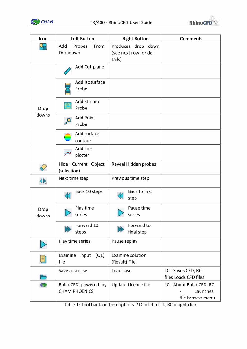
TR/400 - RhinoCFD User Guide
Icon
Left Button Right Button
Comments Name Name
Create Domain To Fit
Object
Deactivate RhinoCFD LC - Starts RhinoCFD and
creates a domain, RC -
Removes domain and CFD
properties
Edit Solution
Parameters
Edit Domain Edge
Properties
LC – Opens the main CFD
setting window
RC – Edit boundary
conditions of domain
Edit CFD Properties Show Table Of Objects LC - Edits currently selected
object
RC – Show list of all objects
Show Grid Dialog
Show Grid Hide Grid
Show Probe Hide Probe
Add User Defined
Functions
Run Solver Display Convergence
Plot
Load Results Remove Visualisation
Edit Display Parame-
ters
Show Scalar Key Hide Scalar Key
TR/400 - RhinoCFD User Guide
Icon Left Button Right Button Comments
Add Probes From
Dropdown
Produces drop down
(see next row for de-
tails)
Drop
downs
Add Cut-plane
Add Isosurface
Probe
Add Stream
Probe
Add Point
Probe
Add surface
contour
Add line
plotter
Hide Current Object
(selection)
Reveal Hidden probes
Next time step Previous time step
Drop
downs
Back 10 steps Back to first
step
Play time
series
Pause time
series
Forward 10
steps
Forward to
final step
Play time series Pause replay
Examine input (Q1)
file
Examine solution
(Result) File
Save as a case Load case LC - Saves CFD, RC -
files Loads CFD files
RhinoCFD powered by
CHAM PHOENICS
Update Licence file LC - About RhinoCFD, RC
- Launches
file browse menu
Table 1: Tool bar Icon Descriptions. *LC = left click, RC = right click

TR/400 - RhinoCFD User Guide
4.3 Main Menu
Figure 6: RhinoCFD Main Menu Window
Button Function Settings of interest
Geometry Settings for grid, coordinate system
and time discretization
Models Specify physical models used for the
simulation
Turbulence, energy, radiation, etc
Properties Specify the fluid properties that
will be modelled in your simulation
Density, viscosity, ...
Initilisation Specify the initial values applied to
your simulations and activate
restarts
Help Launch help
Sources Whole domain sources Gravity, buoyancy and moving/rotating
coordinate systems
Numerics Numerical settings for solution
control
Number of iterations and relaxation
Output Result file sources printout and 3D
solution dumping controls
Probe location, print out of variables, file
dumps and extra derived variables
‘?’ Launches a help window within the
menu. Activate through clicking on
‘?’ then on the any button
Table 2: Main Menu Description

TR/400 - RhinoCFD User Guide
5 Setting up a CFD Model
5.1 Introduction
Having discussed how to install and start RhinoCFD, we are now ready to set up a CFD
model. This section discusses the principal aspects of setting up a model, which will be
addressed in turn:
5.2 Geometry
The geometry of the model is set up in Rhino, and therefore appears automatically in the
RhinoCFD plugin, as shown in this example:
Figure 7: Solution domain around Rhino-generated objects

TR/400 - RhinoCFD User Guide
5.3 Domain
The region of space in which the solution is to be performed is termed the “Solution Domain”.
It is a rectangular region of Cartesian space, as shown for example by the black lines in Figure
7. A default domain is defined when exiting the Start New Case dialog, as described in section
3.1. The domain will automatically be created large enough to encompass all the geometry
that has been set up in Rhino. It can easily be resized if a larger domain is required, e.g. for
an external simulation of wind flow around buildings.
5.4 Mesh
A full discussion of both automatic and manual meshing is given in section 6.
5.5 Boundary Conditions (Flow and Thermal)
The flow conditions and the thermal conditions that characterise the model must be specified.
So for example the following boundary conditions need to be quantified, and their locations
specified:
Inflows or outflows of fluid (see section 9.2).
Fixed-pressure boundaries (see section 9.3).
Fixed-temperature boundaries (see section 8).
Heat sources (see section 8).
Pollution sources.
All the boundary conditions and sources are set up using CFD objects. Section 7 discusses
how these are specified.
5.6 Solution Parameters
The above aspects of setting up a CFD model are all visual, in the sense that they are all
concerned with geometry. Other non-visual parameters are also required to specify the
model, e.g. what equations are to be solved, what is the fluid, what are the solids, what are
the solution controls, etc. These aspects are all set in the “Main Menu” of RhinoCFD. For a
full description of the Menu the reader is referred to the Phoenics VR User Reference Guide.
A brief discussion of the most important parameters which need to be considered when
setting up a model is given in Section 10 below.

TR/400 - RhinoCFD User Guide
5.7 Other Important Aspects of CFD Models
There are some additional important aspects of CFD modelling with Rhino that are important.
These are discussed in the subsequent sections of this guide, as follows.
Use of the Probe (section 11)
Convergence and relaxation (section 12)
Running simulations (section 13)
Running transient models (section 14)
Viewing the results (section 15)
Section 16 describes the use of the Scalar Key in contour and vector plots, and Section 17 lists
and discusses the various files associated with RhinoCFD.
5.8 Steady and Transient Simulations
RhinoCFD can handle both steady and transient simulations.
Steady simulations are independent of time and assume that the boundary conditions are
constant. Examples are a steady ventilation pattern in a building, or steady flow over an
aerofoil.
In a transient simulation, the velocity pattern and the temperature distribution can change
with time. An example of a transient simulation is the development of a fire in a building, to
predict the build-up of the smoke layer, so as to determine the time available for escape.
Transient simulations are computationally more expensive than steady ones.
When you enter RhinoCFD the simulation is set to be steady by default. Section 14 discusses
how to run a transient simulation.

TR/400 - RhinoCFD User Guide
6 Meshing (Affecting the Grid)
6.1 Purpose of Mesh
The principle by which CFD works is to subdivide a domain into many small “control volumes”
known as cells, and then solve the Navier-Stokes equations to obtain values for pressure,
momentum, temperature and other variables at each of these cells. The equations represent
conservation of mass, momentum, energy etc. The more cells you have, the more accurate
the representation of your scenario will be. However, the simulation will take a longer time
to complete and converge, and incur a greater computational expense.
6.2 Available Mesh Types
RhinoCFD uses Cartesian or cylindrical-polar structured meshes which are very easy to set
up, and have lower discretisation error than non-orthogonal or general unstructured
meshes.
6.3 Geometry Detection
RhinoCFD uses a cut-cell method called PARSOL that automatically detects what part of a cell
is solid and what part is fluid, and applies the correct boundary conditions to the relevant
parts of the cell. This means that you don’t need to spend hours defining the mesh so that it
perfectly fits the geometry; just ensure you have a fine mesh and let RhinoCFD do the hard
work.
6.4 Displaying the Grid
Left clicking on the 5th tool bar icon reveals the grid within the current view. Rotate the
perspective view, or click in a different view, to change the grid view. The grid location is
determined by the ‘probe’ (Section 7); move the probe to move the grid around the domain.

TR/400 - RhinoCFD User Guide
Figure 8: Grids Lines
6.5 Grid Regions
The standard Cartesian mesh is formed of regular hexahedral cells stacked in rows and
columns, and is represented in RhinoCFD by means of blue lines which indicate the cell faces.
In each of x, y and z the mesh is divided into a number of ‘regions’ in order to provide detailed
grid control. The size and distribution of the cells within each region can be modified via the
grid dialog menu. The grid lines representing region boundaries are indicated by orange lines
(purple if the object is currently selected); so for example in the above Figure 8 it will be seen
that there are three regions in each of the vertical and horizontal coordinates.
Regions can be created by setting particular objects to ‘affect the grid’ (see Section 7.3), in
which case region boundaries will be inserted at the extremities of the object. Alternatively,
regions can be created by defining a Null object (see Section 7.4). The minimum size of the
each region can be set by modifying the tolerance in the grid dialog.

TR/400 - RhinoCFD User Guide
6.5 Manual and Automatic Meshing
In each coordinate direction (x,y,z) the mesh may be constructed automatically, or with
manual intervention if preferred. This choice may be made separately for each of x, y and z.
The automatic meshing process ensures that the resulting mesh is "well-conditioned" in the
sense that there are no abrupt changes in cell width; on the other hand, the cells may not be
distributed optimally for the specific model. Manual meshing allows the user to distribute
cells more efficiently. This can be a time-consuming process, but one that pays dividends in
terms of the quality of the results.
The default meshing method is automatic. This will therefore be described first.
6.7 Automatic Grid Generation
Figure 9: Grid Mesh Settings Dialog - Automatic
RhinoCFD uses an automatic mesher as the default option. The auto-mesher will always
produce a well-conditioned grid for the geometry being analysed, though the user should
check that the mesh distribution has adequate resolution.
Clicking on X, Y or Z direction buttons brings up the settings dialog for that direction, with
the options explained following Figure 10:

TR/400 - RhinoCFD User Guide
Figure 10: Auto-Mesh Dialog
1. Resets all values to their defaults.
2. Sets the smallest cell size allowed as a fraction of the domain size in that direction. The
default is 0.005.
3. The automatic mesher uses iteration to generate the mesh. This sets the initial cell size
for the iteration as a fraction of the domain size in that direction. The default is 0.05,
which gives roughly 20 cells if the regions are fairly equal in size.
4. Sets the maximum size ratio for adjoining cells in neighbouring regions. For example,
with a ratio of 1.5, the last cell in region 1 cannot be more than 50% wider than the
first cell in region 2 (or vice versa).
5. Sets the expansion/power (see (7)) used to adjust the grid within a region so as to
satisfy the cell-size ratio requirements at the region ends. The default value is 1.2. A
value of 1 will enforce a uniform grid in the region. Increasing the value increases the
degree of crushing the cells towards one end of the region.
6. By default, the minimum and initial cell factors (2 and 3) are set as fractions of the
domain size. When ’Fractions’ is clicked, the setting changes to ’Size’. The minimum
and initial cell sizes are now set as physical sizes in metres.
7. The grid can expand using either geometrical progression, or a power-law expansion.
Geometrical progression gives a uniform expansion in grid size across the region,
whereas using a power law concentrates the expansion towards one end of the region.
8. This allows the user to control whether a one-sided expansion towards the boundary,
or a symmetrical expansion, is applied in the first region in the relevant coordinate
direction. The former corresponds to OFF (default).
9. Similar to (8), but for the last region in the relevant coordinate direction.
Tips for using the Automatic mesher:

TR/400 - RhinoCFD User Guide
The initial cell factor is used as starting point for the number of cells. If you want a large
number of cells, then a use a small fraction or size.
The minimum size of the cell is a limit rather than a determining factor for the grid. This
can be used to ensure that the grid is fine enough at the walls of an object, or ensure all
cells the same size by making it equal to initial cell factor.
Using the fraction option may be helpful for quickly setting up a reasonable grid when the
domain is much larger in one coordinate than in another. Using the sizes options can be
easier for refining complex regions as the input can be directly related to the geometry
dimensions.
The Max size ratio should not be greater than 2; ideally it should not exceed 1.5.
The Low (8) and High (9) options should only be used if it is necessary to resolve flow
details near the domain boundaries. They should be left "Off" for external flows such as
wind flow around buildings.
The user should critically examine the grid before running a simulation, and assess
whether the meshing is adequate to resolve details of complex geometry and flow
features such as recirculation regions.
The Auto-mesher is often very useful for quickly creating a mesh for a complex model with
many objects. The mesh generated will always be well conditioned. However, the user
should check whether mesh resolution is adequate.
6.8 Manual Grid Generation
Figure 11 shows the layout of the grid mesh settings dialog. Each feature is briefly described
here. Further help can be found by clicking on ‘?’ and then on a button. This dialog is accessed
by clicking on ‘Geometry’ in the main menu.
Figure 11: Grid Mesh Settings Dialog – Manual

TR/400 - RhinoCFD User Guide
1. Select either Cartesian or Polar coordinate system.
2. Choose either steady or transient simulation.
3. Change the cut cell method (Only Parsol available currently).
4. Change grid specification to automatic or manual.
5. Display domain size (edit using 9).
6. Total number of cells in each coordinate.
7. Region tolerance - i.e. minimum region width.
8. Total number of regions in each coordinate.
9. Button to edit size, cells, regions and distribution in each coordinate.
Clicking on "X direction", "Y direction" or "Z direction" (9) brings up the following menu.
Figure 12: X Grid Dialog
1. Edit the size of the domain in the current coordinate.
2. Edit the total number of cells in current coordinate, when auto grid is off (Click Apply
to activate change).
3. Turn auto grid on or off.
4. Frees all regions – where not specifically set by the user, the number of cells and the
power/factor in a region cannot be changed unless the region is ‘free’.
5. Edit region tolerance.
6. Edit number of cells in region.
7. Change distribution law – power law or geometric progression.
8. Edit power for power law or factor for geometric.
9. ‘Symmetric’ on/off - i.e. crush both ways.
10. Free individual regions.

TR/400 - RhinoCFD User Guide
6.9 Editing Regions
With complex geometry it is possible to end up with many regions, which can make it hard
to know which region is being edited. To help with this, RhinoCFD highlights the cells of the
region you are editing after you click ‘Apply’.
Figure 13: Example of Editing Regions
6.10 Best Practices
To help those new to CFD get to grips with creating and refining grids, here are a few best
practices:
Grid expansion coefficients should not be greater than 1.3 if power distribution is used,
or 1.1 for geometric distribution, and should not be less than 1.0. Use a negative
coefficient to crush the cells in the opposite direction.
Neighbouring cells should have a width ratio no greater than 2:1, and preferably less than
1.5:1.
Inlets and outlets should always ‘affect the grid’ (boxes ticked in Object Properties).
Objects do not always have to affect the grid, but areas of interest should.
Regions of complex geometry should contain enough cells to ensure that all geometry is
properly detected.
RhinoCFD uses the ‘PARSOL’ feature to handle cut cells where the geometry is angled,
curved or not aligned with cell faces. Cells should not be double cut - no more than one
cut per cell should be seen in any cell.
In the object specification menu, ‘Null’ type objects can be selected which have no effect
but to create additional regions for the purpose of grid control

TR/400 - RhinoCFD User Guide
6.11 Restarting with a Different Grid
It is possible to run a simulation with a small number of cells, and then refine the grid and
restart from where the previous simulation finished. This is possible as the solver
interpolates from the old grid to the new. To activate this feature, run a simulation, change
the grid and then activate restart in the initialisation tab in the main menu (see Section 4.3).
When ‘run solver’ is selected the following warning will appear:
Figure 14: Grid Interpolation Warning
Click yes to continue and the simulation will begin. It is recommend that large changes to the
grid are not made and refinement is made in increments as interpolation works best when
difference is cells is not great.
6.12 Coordinate Systems
Coordinate
System
Description
Cartesian The default grid coordinate system. This is a structured mesh in
which cells stack in rows and columns in the x, y and z coordinate
directions. Cells are 6 sided blocks (hexahedrals).
Cylindrical
Polar
For use where the geometry has significant cylindrical features
with a common axis. Here x must be then circumferential, y the
radial and z the axial coordinate.

TR/400 - RhinoCFD User Guide
Figure 15: Polar Grid
6.13 Cylindrical Polar Simulations
A cylindrical polar grid can be selected on start-up of RhinoCFD by ticking the box next to
‘Domain to use polar grid’.
Figure 16: Start RhinoCFD with a Polar Domain
The grid can also be changed any time after starting RhinoCFD, by left clicking on ‘Show Grid
Dialog’, and then clicking on ‘Co-ordinate system - Cartesian’ brings up the following menu:

TR/400 - RhinoCFD User Guide
Figure 17: Coordinate Selection Menu
Note: the domain may have to be moved to perfectly fit geometry if the coordinate system
is changed after starting RhinoCFD.
TR/400 - RhinoCFD User Guide
7 CFD Objects
7.1 The use of Objects
RhinoCFD uses Rhino-generated geometries, known as CFD objects, which are three-
dimensional geometrical entities. These CFD objects perform specific functions for CFD
simulations, such as defining the geometry, describing fluid inflows and outflows, heat and
momentum sources, etc. CFD objects may be given additional attributes relevant for
specifying the CFD simulation. One set of attributes controls whether the geometrical
extremities of the object are to be taken into account when the mesh is generated; this is
referred to as “affecting the grid”. Another set of attributes attach features such as material
properties, flow rates, heat sources etc. to the object; these can then be used to define
sources and boundary conditions for the CFD simulation.
The objects are created in the standard Rhino environment, and then given the CFD
attributes using the object dialog in RhinoCFD. Special CFD objects, such as Wind, can be
created automatically through using the RhinoCFD menu.
7.2 Creating CFD Objects
Objects are created in the standard Rhino environment, and then given CFD settings using the
object dialog. Special CFD objects, such as Inlets, can be created automatically through using
the RhinoCFD menu.
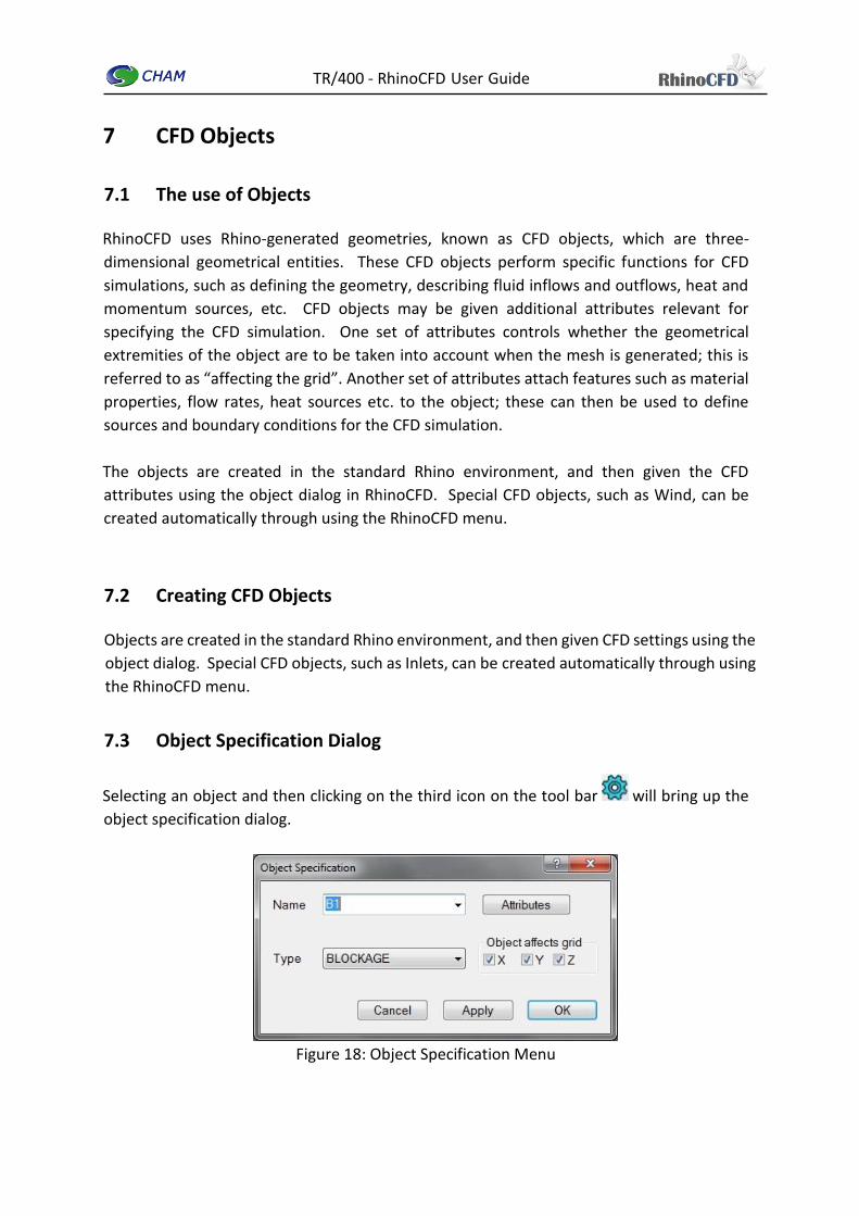
7.3 Object Specification Dialog
Selecting an object and then clicking on the third icon on the tool bar will bring up the
object specification dialog.
Figure 18: Object Specification Menu

TR/400 - RhinoCFD User Guide
This dialog specifies:
The name of the object.
The attributes, i.e. CFD properties - temperature, pressure, velocity, etc.
The type of object: Blockage, Inlet, Outlet etc.
Whether or not the object creates grid regions (“affects the grid”):
It is important to note the following:
Different object types and options have entirely different attribute options.
Appropriate naming of objects will make them much easier to identify both in the Rhino
environment and in the Q1 file (CFD input file - see Section 17.2).
7.4 Common Object Types
Objects created within the Rhino environment will automatically be classed as ‘blockages’
once a domain has been created. This can be changed using the RhinoCFD tool bar to a wide
range of object types using the Object specification menu. The most common object types
are explained in Table 3.

TR/400 - RhinoCFD User Guide
Object
Type
Description Key Settings
Blockage Volume object, used either to specify a solid region or a
fluid region where for example a heat source or
momentum source is located. Default material is "198
Solid", a non-conducting solid.
Material type, heat
sources, porosity,
momentum sources
Inlet Used on the domain boundaries to specify a mass flow
through it, either as an inflow or an outflow.
Mass flow rate, volume
flow rate, velocity
Outlet Used on the domain boundaries to specify a value for
external pressure. Mass flow through it is calculated
automatically based on the difference in pressure near
the outlet and the prescribed value.
External pressure
Angled-in Similar to Inlet, used to prescribe a fixed mass source or
sink within the domain. It must intersect a solid blockage,
lying partially inside it. The area specified as the Inlet is
the plane of intersection between the blockage and the
angled-in.
Mass flow rate, volume
flow rate, velocity
Angled-
Out
Similar to outlet, used to prescribe a fixed pressure region
within the domain. It must intersect a solid blockage, lying
partially inside it. The area specified as the outlet is the
plane of intersection between the blockage and the
angled-out.
External pressure
Wind Covers the entire domain and automatically sets up
boundary conditions for all domain faces based on the
prescribed wind conditions. It also automatically applies
wind profiles and initializes the solution to the prescribed
profile.
Reference
velocity/height,
access to EnergyPlus
database, type of wind
profile, upstream
conditions
Null Used exclusively to set up new grid regions for mesh
control. Does not affect the flow in any other way.
Table 3: Common Object Types
Many more object types are available - please see either Appendix A or Object types in
PHOENICS for more information.

TR/400 - RhinoCFD User Guide
8 Blockage Objects – Heat and Momentum Sources
8.1 Introduction
Blockage objects can be used to represent:
blocked regions which do not conduct heat, and so for which no material properties are
defined (these are known as “198” objects).
blocked regions which do conduct heat, and are made of a particular material with
specified physical properties.
regions of the fluid where something specific is to be specified - e.g. heat or momentum
sources.
The attributes dialog varies, depending on various settings in the RhinoCFD menus, such
as energy models, co-ordinate systems, object types etc. Some important and commonly
used attribute settings are explained here and in the following subsections.
8.2 Non-thermally-conducting ‘198’ Blockage
The default object type for any object drawn in RhinoCFD is the non-thermally-conducting
“198” Blockage; clicking on Attributes brings up the dialog shown in Figure 19.
Figure 19: Default Attributes Menu
The Material setting for this form of Blockage is “198 Solid with smooth-wall friction”; this is
the default setting. Click the relevant buttons if you want to:
Set a Wall roughness.
Select a non-default wall-function.
Specify a ‘slide velocity’ (i.e. if the wall is acting like a conveyor belt).

TR/400 - RhinoCFD User Guide
8.3 Thermally-conducting Blockage
Click the Types button on the Attributes dialog (Figure 20) to bring up a list of material types:
Figure 20: Material Types
Click Solids and select the appropriate material from the list. The purpose of this is to specify
the properties of the material (density, specific heat, thermal conductivity etc.). The
numerical values for the various materials are listed in Appendix C to this Guide. If you need
a material with properties different from the materials in the list, you can easily specify these
using the InForm feature.
When a solid material is selected, the Blockage Attributes panel will look like this:
Figure 21: Blockage Attributes

TR/400 - RhinoCFD User Guide
In this example aluminium has been selected. ‘100’ is the index number of aluminium in the
materials list. Click the relevant buttons in the Attributes panel if you want to:
Set a wall roughness
Select a non-default wall-function law
Specify a “Slide velocity” (i.e. if the wall is acting like a conveyor belt)
It is possible to apply a heat source to a thermally-conducting Blockage, once solution of the
energy equation has been switched on in the Models section of the Main Menu. Clicking on
Energy Source in the Attributes dialog will produce the following panel, where the type of
energy source may be selected:
Figure 22: Energy Source Menu
These options are described in Section 5.6 below.
8.4 Source Region in the Fluid
If the Blockage is intended to demarcate a region of the gas or liquid where a heat source or
momentum source (for example) is to be applied, you should click the Types button on the
Attributes panel to bring up the list shown in Figure 20 and then select Domain Material from
the list. The term “Domain Material” describes the type of fluid flowing in the domain, as
explained in section 10.4.1.
The Attributes dialog will now be as shown in Figure 23.

TR/400 - RhinoCFD User Guide
Figure 23: Domain Material Settings
It is possible to apply a heat source to a domain-material Blockage, once solution of the
energy equation has been switched on in the Models section of the Main Menu. Clicking on
Energy Source in the Attributes dialog will give the following options explained in the table
below:
Energy Source Description
Fixed temperature The temperature throughout the volume of the object is
fixed to the specific value
Fixed Heat Flux A heat flux throughout the object is specified, with the set
value. The value can be specified as a total flux for the
object, or as a flux per unit volume (units W or Wm3).
Adiabatic There is no heat source. This is the default setting for a new
object
Linear Heat Source The heat source in any cell within the object is calculated
from the expression Q = Vol × C(V − Tp) where V is an external
temperature with units K or ◦C, C is a heat transfer coefficient
with units W/m3K, Tp is the local cell-centre temperature and
Vol is the cell volume.
Table 4: Commonly used energy source options
You can specify, within the region occupied by the Blockage, the velocity (m/s) or a force on
the fluid (N), specified as three Cartesian components. Clicking on Momentum Source will
produce the following panel, where the type of energy source may be selected:

TR/400 - RhinoCFD User Guide
Figure 24: Momentum Source Dialog
These options are defined in the following table:
Momentum Source Description
Fixed Velocity The velocity throughout the volume of the object is fixed to
the specified value
Fixed Momentum
Flux
The momentum flux (force) throughout the volume of the
object is fixed to the set value. The value is specified as a total
force in Newtons for the object
None There is no driving force. This is the default setting for a new
object
Linear Source The force in Newtons is calculated from the expression F
=mass-in-cell × C (V − Velp). Where C and V are user-defined
constants with units of 1/s and m/s respectively and Velp is
the velocity in any cell within the object
Table 5: Commonly used momentum source options

TR/400 - RhinoCFD User Guide
9 Specifying Inflow and Outflow
9.1 Introduction
Inflows or outflows can be specified in two ways; either as a specified flow rate or as a fixed
external pressure. With the latter, the flow rate is adjusted automatically to match the
specified external pressure, and to balance the other flows in the system.
Sections 9.2 and 9.3 describe how such inflows and outflows may be specified in RhinoCFD.
Section 9.4 discusses when you should specify a fixed flow rate and when a fixed pressure.
9.2 Fixed Flow Rate Sources
9.2.1 Fixed Flow Rate Sources on the Domain Boundary (Inlet)
To specify a fixed flow rate (i.e. inflow or outflow) at the domain boundary, an "Inlet" object
should be used. The flow rate may be specified in one of the following ways:
Cartesian velocity components (m/s)
Volume flow rate (m3/s)
Mass flow rate (kg/s)
If there is a flow through an entire face of the domain, this is easily specified in RhinoCFD
using the Domain Faces menu, which is accessed by right-clicking on the second toolbar icon
.
The following panel shows the attribute settings for Inlet objects.

TR/400 - RhinoCFD User Guide
Figure 25: Inlet Attribute Settings
Note the following:
You can select the flow definition method - velocity components, mass flow rate, volume
flow rate.
Positive values for mass and volume flow rate indicate flow into the domain, negative
values extract fluid from the system.
Positive and negative values for velocity represent the direction of the flow in relation to
the Cartesian coordinates.
The temperature at Inlet is either user-set or “ambient” (default) - note that the ambient
temperature value is set in the Properties panel of the Main Menu.
If scalars are solved (e.g. pollutant concentrations), appropriate values must be set at
every Inlet.
The turbulent intensity at the Inlet, the density of the inflowing fluid, and the net area ratio
for inflow through a grille may also be set. Details of these options may be found at TR326-
Inlet.

TR/400 - RhinoCFD User Guide
9.2.2 Fixed Flow-rate Sources within the Domain (Angled-in)
To specify fluid entering or leaving within the domain, you should use an ‘Angled-in’ object.
An Angled-in is used to define a region of fixed flow rate, either in or out. The region of
influence is the part of the surface of any blockage object(s) enclosed by the Angled-in object.
An Angled-in is used to delineate the part(s) of the surface of an internal blockage where
flow is entering the system from the blockage, or being extracted from the system into the
blockage. An Angled-in should be placed such that it overlaps the blockage, to create an
inter-sectional region. The amount that the object protrudes from the blockage is not
important, but it is recommended that the Angled-in extends at least one cell in thickness
either side of the blockage surface.
An example of an Angled-in is shown here.
Figure 26: Example of use of Angled-in
The flow-rate through an Angled-in may be specified in one of the following ways:
Cartesian velocity components (m/s)
Normal velocity (m/s)
Volume flow rate (m3/s)
Mass flow rate (kg/s)

TR/400 - RhinoCFD User Guide
The “Normal velocity” option allows the user to specify the velocity normal to the surface of
the underlying blockage. If the mass or volume inflow is specified, the direction of the inflow
will be normal to the blockage surface.
The following panel shows the Attributes settings for Angled-in objects. They are very similar
to the attribute settings for Inlets, described previously.
Figure 27: Angled-In Attribute Settings
9.2.3 Linked Angled-ins
A feature specific to the Angled-in objects is the linking feature displayed at the top of the
attributes panel. This can be used to represent the flow through a piece of equipment within
the domain which is not modelled in detail, but is represented by a blockage. To do this we
use a pair of linked Angled-in objects.

TR/400 - RhinoCFD User Guide
Figure 28: Linked Angled-ins
For example consider an induction fan, where the air is sucked in on the underside of the fan
and then blown out sideways at an angle. An Angled-in can be used to represent the suction
into the fan; here the suction rate is specified. The nozzle of the fan is represented as a
second Angled-in, linked to the first; the linking ensures that the mass flow rates for the
outflow nozzle and for the suction balance, and that the temperatures (and any other scalars
such as smoke concentration) balance likewise. It is this linking of the temperatures at the
suction side and at the nozzle for which the linking feature is required. An additional heat
source can be specified if desired, representing any extra heating or cooling taking place.
Alternatively, the exit temperature can be specified, or the temperature rise (or fall) can be
specified.
The mass flow is set at the suction Angled-in, and the temperature and the other scalars are
based on the average values of the air sucked in. The ‘nozzle’ Angled-in should be linked to
the suction Angled-in. The velocity at the nozzle will be deduced from the mass flow rate
and the area. If the density is set to use the Ideal Gas Law (in the Properties section of the
Main Menu), the density at the nozzle will be evaluated at the mean temperature of the air
passing through the nozzle.
More information is available on Angled-ins at TR326 - Angled-in.
TR/400 - RhinoCFD User Guide
9.3 Fixed Pressure Sources
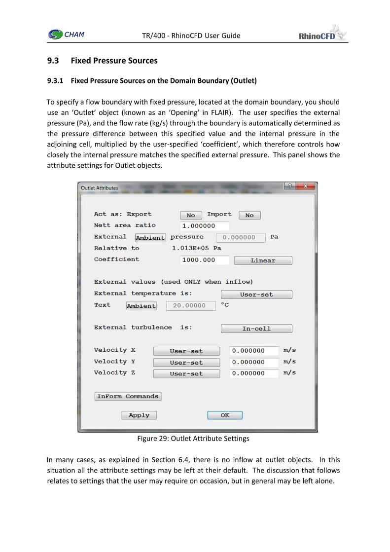
9.3.1 Fixed Pressure Sources on the Domain Boundary (Outlet)
To specify a flow boundary with fixed pressure, located at the domain boundary, you should
use an ‘Outlet’ object (known as an ‘Opening’ in FLAIR). The user specifies the external
pressure (Pa), and the flow rate (kg/s) through the boundary is automatically determined as
the pressure difference between this specified value and the internal pressure in the
adjoining cell, multiplied by the user-specified ‘coefficient’, which therefore controls how
closely the internal pressure matches the specified external pressure. This panel shows the
attribute settings for Outlet objects.
Figure 29: Outlet Attribute Settings
In many cases, as explained in Section 6.4, there is no inflow at outlet objects. In this
situation all the attribute settings may be left at their default. The discussion that follows
relates to settings that the user may require on occasion, but in general may be left alone.

TR/400 - RhinoCFD User Guide
The Attributes menu provides options to:
Set the external pressure - this is defaulted to zero, and should usually be left at zero. This
zero represents pressure relative to a reference pressure, usually taken to be atmospheric
pressure. This reference pressure may be set in the Properties section of the Main Menu.
Set the temperature of the inflowing fluid - either User-set or Ambient (default). Note
that the ‘ambient’ temperature may be set in the Properties panel of the Main Menu.
Set the value of any scalars (e.g. pollutant concentrations) of inflowing fluid.
There may be inflow, or outflow, or both, at an Outlet/Opening. The temperature and
scalar settings are only relevant for inflow. The velocity settings are likewise only relevant
for an inflowing fluid. These are only required by advanced users; guidance may be found
in TR336-Outlet.
If the pressure is fixed over an entire face of the domain, this is easily specified in RhinoCFD
using the Domain Faces menu, which is accessed by right clicking on the second toolbar icon
.
9.3.2 Fixed-Pressure Sources within the Domain (Angled-out)
‘Angled-out’ objects are exactly analogous to Angled-in objects, as described previously in
Section 6.2.2, except that instead of fixing the flow rate, the external pressure is fixed. The
options available are the same as for Outlet objects described in Section 6.3.1, and as for
Outlets, in many cases all the attribute settings may be left at their default values.
Angled-out objects cannot be linked in the same way as Angled-ins.
9.4 When to Use Fixed-Flow / Pressure Conditions
This section discusses when to use fixed-flow conditions (i.e Inlets or Angled-ins) and when
to user fixed-pressure conditions (i.e. Outlets or Angled-outs, or Openings in FLAIR). The
references here will be to Inlets and Outlets, but the same considerations apply to Angled-
ins and Angled-Outs.
This is best discussed by giving some examples:

TR/400 - RhinoCFD User Guide
If possible there must be at least one Outlet (or Angled-out) object, to provide a pressure
reference for the solution domain. At this Outlet, the pressure should generally be set to
zero.
If there are no inflow or outflow boundaries, there must be a Pressure_relief object (See
Appendix A) to provide the pressure reference.
For a through-flow situation, i.e. with flow entering at one end of the domain and leaving
at the other, we would generally recommend fixing the flow rate (using an Inlet) at the
inflow end and fixing then pressure (using an outlet) at the outflow end. The solution will
ensure mass continuity, i.e. it will force the mass outflow rate to be equal to the mass
inflow rate.
Suppose that there are a number of air supply vents and a number of air extracts, all with
known mass flow rate. As stated above, one of these should be represented as an
Outlet/Opening. The others can be Inlets with the appropriate mass flow rates specified.
The solution will ensure that the mass flow rate for the Outlet/Opening balances mass
continuity
You may have a situation where you know the pressures, but the flow rates are unknown.
For example in a naturally-ventilated building, the air flow will be driven by the pressures
at the open windows and doors; and the objective of the study may be to determine the
ventilation flow rate. In this situation, all the open windows and doors should be
represented as Outlets/Openings. The pressure values at these Outlets/Openings will
need to be specified. They might typically be taken from the results of an external CFD
simulation.

TR/400 - RhinoCFD User Guide
10 Solution Parameters
10.1 Introduction
The aspects of setting up a CFD model which have been discussed above are all visual, in the
sense that they are all concerned with geometry. Other non-visual parameters are also
required to specify the model, e.g. what equations are to be solved, what is the fluid, what
are the solids, what are the solution controls, etc. These aspects are all set in the “Main
Menu” of RhinoCFD. For a full description of the Menu the reader is referred to Section 9 of
the Phoenics VR User Reference Guide . A brief discussion of how to set the most important
parameters is given in here.
To access the Main Menu, click the icon in RhinoCFD. The Menu contains the following
sections:
Geometry
Models
Properties
Initialisation
Sources
Numerics
Output
Domain Faces
The basic aspects of these are discussed in turn in the following subsections.
10.2 Geometry
This takes you to the “Grid Mesh Settings” panel, which can alternatively be accessed by
clicking .
10.3 Models
In this panel the user can specify which transport equations are to be solved. A full description
may be found here. In this section the most commonly used options are described.

TR/400 - RhinoCFD User Guide
10.3.1 Solution for temperature
Solution for temperature can be switched on and off.
10.3.2 Turbulence Models
A large number of turbulence models are available in RhinoCFD. The complete set of models
are described in the POLIS Encyclopaedia under Turbulence, where each has its own
descriptive article. The turbulence models most likely to be of interest to the RhinoCFD user
are the following.
Turbulence model Description
LAMINAR The flow is laminar and there is no turbulence model.
KEMODL The classic two-equation k-epsilon model.
KECHEN The default model. Chen-Kim improvement to the two-
equation k-epsilon model. Gives better prediction of
separation and vortices than the classic k-epsilon.
KEREAL Realisable k-epsilon. Gives better prediction of separation
and vortices than the standard k-epsilon.
KERNG RNG-derived two-equation k-epsilon model. Like
Chen-Kim it gives improved prediction of separation
and vortices. However, the user is advised that the
model results in substantial deterioration in the
prediction of plane and round free jets in stagnant
surroundings.
LVEL A zero-equation algebraic model based on distance from the
wall. Good for channel flows and “cluttered” spaces where
there is not enough mesh to resolve boundary layers properly.
Table 6: Turbulence Models in RhinoCFD
10.3.3 Radiation
The “Immersol” radiation model can be switched on and off. This is an economical but
approximate diffusion-based model. Theoretical details may be found here.

TR/400 - RhinoCFD User Guide
10.3.4 Variables
The “Solution control / extra variables” button enables quick review of which variables are
being stored, and which solved, and by what method. Here a “variable” means a quantity
which has a value stored at every cell in the domain; and a variable being “solved” means
that the variable is a conserved quantity which is subject to a transport equation.
The Y/Ns are toggles, Y indicating Yes and No; clicking on one changes Y to N or vice versa.
The top line "SOLUTN 1 STOR" indicates whether or not each variable is stored. They are all
Y, because if you click one to change it to N, that variable is no longer stored, and it disappears
from the table.
The second line "SOLUTN 2 SOLV" indicates whether or not each variable is solved (i.e. has a
transport equation which is solved).
The third line "SOLUTN 3 WHOF" indicates whether the linear solver for the variable is the 3D
whole-field solver (Y), or the 2D slab-by-slab solver (N). Pressure, temperature and scalar
variables such as pollutants or smoke should always be solved whole-field.
To solve an additional transport equation, e.g. for a pollutant such as CO, type CO in the
“SOLVE” box and click Apply. Be sure to set CO to be solved whole-field.
10.3.5 AGE
This enables solution for a variable AGE which represents the mean age of air since entry to
the domain. Regions with high values of AGE can be useful to indicate poorly-ventilated
regions.
10.4 Properties
10.4.1 Domain Material
The term “Domain Material” describes the type of fluid flowing in the domain. It may be set
to any of the gases or liquids listed by clicking “Gases” or “Liquids”, but almost always one
of the following will be appropriate.

TR/400 - RhinoCFD User Guide
Gases
0 air modelled as incompressible
2 air modelled as compressible using the ideal-gas law
Liquids
67 water
For gases numbers 0 and 2 listed above, note that these numbers not only indicate that the
fluid is air, but also what density formulation is to be employed.
10.4.2 Reference Pressure
When using RhinoCFD the pressure at one or more of the fixed-pressure boundaries
(“Outlets”) should generally be set to zero. This represents the pressure relative to
atmospheric; the absolute value of this pressure reference should be set here (default value
101325 Pa).
10.4.3 Reference Temperature
This should be 0 if working in degrees C, 273 for degrees K.
10.4.4 Ambient Temperature
The ‘Ambient temperature’ setting is be used for two purposes:
to initialise the temperature at the start of a simulation (only if “Initialise from ambient”
is set),
to specify the temperature at which the reference density is set, the latter being used in
specification of the buoyancy force (only if “Set buoyancy from ambient” is set). See
section 10.4.6 “Sources”.
The “Initialise from ambient” temperature setting enables easy specification of the reference
density, and so is generally advisable when there are temperature variations. Note that the
ambient temperature does not necessarily represent the temperature of external air. For
flow within a contained space, it should generally be a typical value of the temperature
within the space.

TR/400 - RhinoCFD User Guide
10.5 Initialisation
Here the initial value may be specified for each variable. The variable is set to this value over
the whole domain at the start of the iteration.
Generally, it is not necessary to select initial values in a steady (i.e. time-invariant) simulation.
An exception is temperature, but this is initialised automatically if “Initialise from ambient” is
selected in the “Properties” menu (see 10.4.4).
In transient solutions it is very important to set the initial conditions.
In general, the principal use of the Initialisation menu will be to:
Select “Activate restart for all variables”, to specify a restart run, i.e. to continue the
solution from a previous run - “Name of restart file” specifies which file is to be used for
the restart data; or to
“Reset initial values to default” to undo this and start afresh.
10.6 Sources
This panel allows the creation of whole-domain sources, which are not attached to any
specific object. All sources or boundary conditions which do not apply to the whole domain
must be attached to an object, and set through the appropriate object attribute dialog box.
A full description may be found here. In this section the most commonly used options are
described.
10.6.1 Gravitational Forces
Here you may switch these on or off.
10.6.2 Buoyancy Model
The most frequently used models are the following.
Constant - Applies the full gravitational force.
Density Difference – Bases the buoyancy force on a density which has a “reference
density” subtracted. This has the effect of removing the hydrostatic pressure gradient.
Boussinesq Approximation – Bases the buoyancy force on temperature difference rather
than density difference. Can be used with constant-density setting. Only use for small
temperature variations.

TR/400 - RhinoCFD User Guide
All are described in the Encyclopaedia under Gravitational body forces. If ‘Set buoyancy from
ambient’ on the Properties panel (section 10.4.4) is set to ON, the reference density will be
computed from the ambient temperature set in the Properties panel.
10.6.3 Gravitational Acceleration
This allows you to set the cartesian components of the gravitational force vector. The
cartesian z-axis is commonly taken as the vertically upwards direction. For this reason the
default setting for gravitational force vector is (0, 0, -9.81).
10.6.4 Reference Density
This can only be set here if “Set buoyancy from ambient’ on the Properties panel (section
10.4.4) is set to OFF.
10.6.5 Buoyancy Effect on Turbulence
In turbulent flows, gravity interacts with density gradients to affect the turbulence. In stably-
stratified flows (dense below light), turbulence is damped; in unstably-stratified flows (light
below dense), turbulence is augmented. Clicking this to ON introduces terms which take this
effect into account. These terms are not included by default, as they can have an adverse
effect on the stability of the simulation. For situations with temperature stratification it can
be advisable to switch on this option.
10.7 Numerics
This is where you set the total number of iterations (“sweeps”) for the simulation. Typically,
thousands of iterations may be necessary for full convergence to be achieved.
We sometimes recommend reducing the “Global convergence criterion” from 0.01 to 0.001,
as this can prevent premature cut-off of the solution.
If changes to the relaxation parameters are required (see Section 13), these may be set in the
“Relaxation Settings” panel accessed from the “Relaxation control” button.
10.8 Output
Full details of the extensive output settings and controls may be found here. This section
describes a few of the most commonly useful settings.

TR/400 - RhinoCFD User Guide
At the top of the Field Printout Settings panel there is a check-box labelled “Suppress all
field printout”. This should always be checked. It eliminates non-essential output to the
Result file, thereby enabling attention to be focussed easier on the convergence
information.
NPRINT (in the Field Printout submenu) controls the frequency in sweeps of the Nett
Source printout to the Result file. While this is not essential, it is often useful. Setting
NPRINT to 250 may be a convenient value.
It can be useful to specify intermediate field dumps at regular intervals. This is achieved
from the Field Dumping submenu, by setting Intermediate field dumps to ON, and then
specifying the frequency for the dumps.
10.9 Domain Faces
Figure 30: Domain Face Settings
The Domain Faces panel allows boundary conditions which apply to entire faces of the
domain to be set up rapidly.
TR/400 - RhinoCFD User Guide
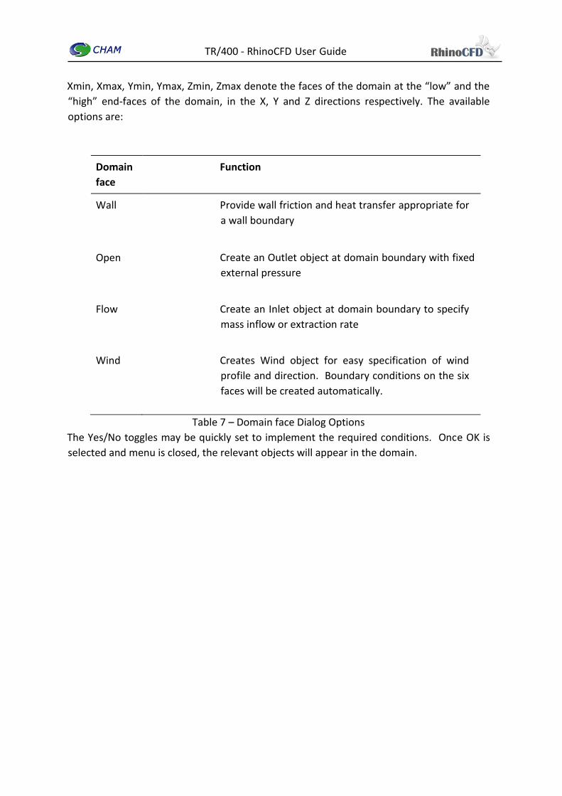
Xmin, Xmax, Ymin, Ymax, Zmin, Zmax denote the faces of the domain at the “low” and the
“high” end-faces of the domain, in the X, Y and Z directions respectively. The available
options are:
Domain
face
Function
Wall Provide wall friction and heat transfer appropriate for
a wall boundary
Open Create an Outlet object at domain boundary with fixed
external pressure
Flow Create an Inlet object at domain boundary to specify
mass inflow or extraction rate
Wind Creates Wind object for easy specification of wind
profile and direction. Boundary conditions on the six
faces will be created automatically.
Table 7 – Domain face Dialog Options
The Yes/No toggles may be quickly set to implement the required conditions. Once OK is
selected and menu is closed, the relevant objects will appear in the domain.

TR/400 - RhinoCFD User Guide
11 The Probe
The Probe is a marker, shown as in RhinoCFD, which can be positioned by the user
anywhere in the domain.
When setting up a model, the probe represents the location which will be used to monitor
the convergence of the solution. The probe will initially appear at the centre of the domain.
It may be repositioned by the user as desired.
When post-processing the results of a simulation, the probe may be used to extract the
values of the variables at a particular point.
Here are some useful tips about using the probe:
The probe should preferably be located out of the mainstream flow, perhaps in the wake
of an obstacle; preferably downstream rather than upstream, and not adjacent to any
boundary.
The probe should not be located inside a solid.
Viewing the probe – the location of the probe can be found easily by left-clicking on the
toolbar icon .
The probe can be hidden by right-clicking on the same icon.
While viewing the grid and the results, the current plotting plane passes through the
probe position; therefore, the viewing plane can be changed by moving the probe.
It is important to note that the position of the probe will not affect the simulation in any way.
It is a tool for investigating and monitoring simulations.

TR/400 - RhinoCFD User Guide
12 Running Simulations
12.1 Starting a Simulation
To run a simulation, left click on the ‘run solver’ icon in the RhinoCFD toolbar:
If you have a sequential-only licence, this will begin the simulation. If on the other hand you
have a parallel licence, the following screen will appear asking for the number of processors
on which to run the simulation; automatic domain decomposition is recommended.
Figure 31: Run CFD Solver Settings
Clicking on ‘Run’ will start the simulation and the convergence monitor plot will appear.
Monitor plots can be used to track the convergence of the simulation, as explained in the
next section. When the simulation is completed the monitor plot will close and the results
can be viewed. For information on convergence see section 13.
12.2 Monitor Plots and Interactive Options
The monitor plot is launched when a simulation is running. It gives real time graphical and
numerical data indicative of the convergence of the simulation. The monitor plot screen can
be used to edit settings during a simulation without changing the Q1 file. Pressing any
character key pauses the run, and displays the in-run options menu as shown in Figure 32.

TR/400 - RhinoCFD User Guide
Figure 32: Monitor Plot Menu
The action of the buttons is as follows.
Reset – change relaxation settings / number of sweeps.
Dump – dump data from current iteration; this can then be viewed graphically.
Monitor – change probe position of the probe / change window width / toggle monitor
plot type.
Endjob – End simulation and dump all data from current run.
Abort – End the run without saving any data from simulation.
Go – End pause, continue with simulation.
Figures on – Toggle figure on or off.
End pause off – Setting to leave the convergence monitor on screen after run is
completed.
Toggling the monitor plot type allows access to a plot of Maximum Absolute Corrections,
which is another useful indicator of convergence (see section 12.1.1).

TR/400 - RhinoCFD User Guide
13 Convergence and Relaxation
13.1 Introduction
A CFD simulation involves solving conservation equations for variables such as mass,
momentum and energy. These equations are highly nonlinear, and as a result have to be
solved by an iterative procedure. It is essential that during the iterative process the solution
will “converge”, meaning that the variables tend towards asymptotic values, and the errors
in the equations reduce in size and (hopefully) become very small. The idea is that after a
certain number of iterations (dependent on the complexity of the simulation) the process
will converge to a solution in which all equations are satisfied with minimal error.
Figure 33: Spot Value and Residuals Plot (Steady Simulation)

TR/400 - RhinoCFD User Guide
Figure 34: Maximum Absolute Correction Plot (Steady Simulation)
If the relaxation controls are set inappropriately, the solution may diverge – this is a kind of
vicious circle in which the variables chase each other to infinity. This is what the CFD
modeller does not want to see. This section discusses how to recognise convergence and
avoid divergence, and how to assess when a simulation is adequately converged.
Figure 33 shows a typical example of the convergence process. The left-hand curves show
the values of the variables at a given location (the probe) converging asymptotically to a
solution; and the right-hand curves show the errors diminishing. In these plots, each
coloured curve represents one of the equations.
This section explains how to assess whether your run is converging, and how to use a
technique known as “Relaxation” to ensure that it does converge.

TR/400 - RhinoCFD User Guide
13.1 Checking Convergence
13.1.1 Method 1 - Use of Graphical data during simulation
Locate the probe somewhere ‘interesting’ – downstream from the inlet and away from
solids. (See section 10.) When running simulations, check out the graph for ‘spot values’ on
the left hand side. When all the variable lines become horizontal, it means that the run is
converged. On the right is another plot labelled ‘% Error’; this is a logarithmic plot showing
the sums over the whole field of the imbalances in variable flows on a cellwise basis. The
curves in the right-hand plot may show irregularities, but should show a steady fall. This fall
in the errors, coupled with stabilising of the values in the left-hand plot, are indicative of
convergence. The simulation will terminate if the lines on the right-hand plot all fall below
the horizontal axis, the height of which is set by a variable RESFAC in the “Numerics” menu.
If the % Error values fall below 1% for all variables, convergence may generally be deemed
acceptable.
Two examples of convergence monitor plots which show good convergence characteristics
can be seen in Figures 33 and 34; these are typical for steady and for transient runs
respectively.
Figure 35: Spot Value and Residuals Plot (Transient Simulation)

TR/400 - RhinoCFD User Guide
Alternative convergence plots can be selected, namely the maximum absolute correction of
each variable in the domain (which ideally should tend to zero) and the maximum and
minimum values of each variable in the domain, which should become stable values.
13.1.2 Method 2 – Reviewing the Nett Sources
Further and more detailed information about the level of convergence can be found in the
“Result” file, accessible from the toolbar or from your working directory. In it you will find
quantitative information regarding the residual errors - and, most importantly, “Nett Source”
information, which lists the following information for each variable:
Inflow rate for each fixed-inflow object (kg/s for mass R1, W for heat flux TEM1)
Outflow rate for each fixed-outflow object (kg/s for mass R1, W for heat flux TEM1)
For each fixed-pressure object, mass inflow and outflow rates plus average temperatures
Total inflow rate for all objects (“pos. sum”)
Total outflow rate for all objects (“neg. sum”)
“Nett sum”, indicating total in/outflow for the variable for all objects
For good convergence, the nett sums should be several orders of magnitude smaller than
the individually itemised flow rates.
It is good practice to check the nett sources for mass (R1) and temperature (TEM1), as well
as for any variables representing pollutants or smoke, both to check convergence, and to
check that all the specified mass, heat and pollutant sources are being recognised.
Figure 36: Sources and Sinks in Result File

TR/400 - RhinoCFD User Guide
Note that if the Nett sums of R1, TEM1, pollutants etc. are not small, then the run is not
converged. But these sums being small is not a sufficient condition for convergence – you
have to check the graphical plots as well (see above).
13.2 Relaxation
The most widely-known technique for achieving convergence is the use of “Relaxation”. This
has an effect akin to damping, and slows down (relaxes) the changes made to the variables
from one iteration to the next. It is important to note that relaxation does not alter the final
solution of the equations, only the way that that solution is achieved.
Two types of relaxation are available - linear (“LINEAR”) and false-time-step (“FALSDT”).
Here we will not look at the theory behind these, just at their practical application.
Relaxation is a big subject, and only an outline guide will be given here.
When you set up a model in RhinoCFD, an automatic convergence tool known as “Conwiz” is
employed. This sets up the relaxation parameters based on a user-set reference velocity and
length scale, and applies linear relaxation to each of the variables. It also limits the maximum
increment of a variable between sweeps, and applies further internal relaxation to the
pressure-correction equation. However this automatic tool is sometimes over-conservative,
leading to run times which are longer than they need be. Some experimenting with manually
set relaxation parameters can therefore pay dividends. The default length and velocity scales
are 1 metre and 10 m/s. If these are inappropriate for the model in question, they should
be reset to more representative values before trying manual relaxation.
To activate manual relaxation, enter the main menu, click on Numerics and then on
Relaxation control. “Automatic Convergence control” should be switched off. You will then
see that each variable has a “RELAX” method (LINEAR or FALSDT) and a “VALUE”. Describing
this in detail is a complex topic, so here we will discuss only the basics.

TR/400 - RhinoCFD User Guide
Figure 37: Relaxation Settings
Relaxation for the pressure P1 is set to LINEAR with a value of 1 - do not change this. The
velocities U1, V1 and W1 should be set to FALSDT, and the value (i.e. the relaxation
parameter) should be set to a typical characteristic time for the flow, in seconds. Often a
suitable value may be found by estimating how long the flow might take to flow through a
single cell in a region where the mesh is fairly fine. In other words, take a typical flow velocity
in m/s, and divide it by the width of one of the smaller cells (in metres). Use the same
number for all three velocity settings. For air flow in and around buildings, we often find
that a FALSDT value of 0.1 seconds is satisfactory.
For temperature, if there are thermally conducting solids present, use LINEAR with a value
of perhaps 0.3. If there are no conducting solids you can do the same, or use FALSDT with
the same numerical value as for the velocities.
The relaxation for the turbulence variables (i.e. the turbulence kinetic energy KE and the
dissipation rate EP) should be left unchanged.
More information on convergence can be found here.

TR/400 - RhinoCFD User Guide
14 Transients
14.1 Introduction
RhinoCFD can handle both steady and transient simulations.
Steady simulations are independent of time and assume that the boundary conditions are
constant. Examples are a steady ventilation pattern in a building, or steady flow over an
aerofoil. It is important to be aware that in a steady simulation, the iterative solution process
does not represent the actual physical time-development of the flow.
In a transient simulation, the velocity pattern and the temperature distribution can change
with time. An example of a transient simulation is the development of a fire in a building, to
predict the build-up of the smoke layer, so as to determine the time available for escape.
Transient simulations are computationally more expensive than steady ones.
When you enter RhinoCFD the simulation is set to be steady by default.
14.2 About Transient Runs
It is important to note the following.
A transient run is solved as set of time steps.
Each time step is iterative and requires sweeps.
Convergence curves are displayed for every time step.
The time steps form a “grid” in time.
There must be enough time steps to adequately resolve process being modelled.
A transient run might typically require one or several hundred steps.
It is generally helpful if the time steps are uniform, although this is not necessary.
The solution uses “implicit” differencing - there is therefore no theoretical limit on step
size.
However, larger time steps may compromise accuracy.
14.3 Setting up a Transient Model
14.3.1 Changing From Steady to Transient
In order to switch from steady to transient, enter the Main Menu by clicking . Click on
Geometry, and then on the button that says ‘Steady’. It will change to “Transient”, and an
extra button to edit time step settings will appear.

TR/400 - RhinoCFD User Guide
14.3.2 Setting time step duration
In the Time Step Settings panel, to set the real time length of your simulation, input your
desired value in seconds into the box labelled “Time at end of last step”.
Enter the number of time steps required for the simulation into the box labelled “Last step
number”, and then click “Apply”. This divides the total time for your simulation by the total
number of steps and thus defines the size of your time step.
Figure 38: Time Step Settings
14.4 Setting Initial Values
In steady-state simulations the initial values serve only to give the solution an initial guess to
start the iteration. In a transient, however, the initial values represent the initial state of the
system, which is of vital importance in determining how the system evolves in time
thereafter.
If the initial state can be specified using uniform values for velocity, temperature and all the
variables, then the appropriate values can be entered in the “FIINIT” boxes of the
“Initialisation” panel of the Main Menu. See Appendix B Variables for an explanation of
the individual variables.

TR/400 - RhinoCFD User Guide
Figure 39: Initialisation Menu
Sometimes, however, the initial state might have non-uniform velocities or temperatures.
For example, you might wish to simulate how flow over a cylinder sheds vortices. In such a
situation you would first need to perform a steady simulation of flow over the cylinder, to
obtain a velocity field from which to start the transient simulation.
To do this, run the steady simulation, and then save the files by left-clicking . You will be
asked to provide a file name; this will apply to all the files created, with different extensions.
The solution file from which the transient is to be restarted will be named <filename>.pda
(where <filename> is the name you provided when saving), and this will need to be entered
in the “Name of restart file” box in the “Initialisation” panel of the Main Menu for the
transient run. Note that “Restart cut-cell values” should be set to NO.
14.5 Number of Sweeps
A typical steady solution might require several thousand sweeps (iterations). However, a
typical transient run might need only 20 to 50 sweeps per time step. This is because in a
short time (such as a single time step) nothing can change very much. If more than 100
sweeps are required to converge the individual time steps, you should consider using a
shorter time step. The total computational expense of the solution is proportional to the
number of time steps multiplied by the number of sweeps. So if you increase the number of
time steps, but thereby reduce the number of sweeps per step, this may not have a
significant effect on the overall run time.

TR/400 - RhinoCFD User Guide
The number of sweeps per step is set in the “Numerics” panel of the Main Menu (obtained
by clicking ).
Figure 40: Numerics Menu (Transient Option Enabled)
14.6 Saving Time Step Results
In a steady solution, the results of interest are produced at the end of the solution, after the
iteration has converged. Intermediate results have no physical meaning, and may only be
interesting insofar as they may be helpful in indicating convergence.
In a transient simulation, the development of the flow with time is likely to be of interest,
and to obtain this from the solution it is necessary to dump intermediate results, i.e. to save
them into your working directory.
To do this, enter the main menu (left-click ) and click on ‘Output’ and then ‘Field
dumping’. In “Step frequency” enter the interval (in time steps) at which you wish dumps to
be produced. Bear in mind that the files produced may be large, and a large number of them
can require a very large amount of disc space. ‘Start letter for solution file name’ specifies a
prefix letter for the intermediate solution files. This can help keep track of the files produced
from different runs.

TR/400 - RhinoCFD User Guide
Figure 41: Dump Settings
In order to organise the transient results, it is recommended that after each simulation the
results are saved to a separate folder. This is done by left-clicking on the second-to-last
toolbar icon . These results can then be loaded into Rhino later, and viewed by right-
clicking on the same icon and navigating to the desired folder.
14.7 Convergence and Relaxation for Transient Runs
The transient term in the equations has a stabilising effect akin to relaxation. This may be
understood intuitively by realising that in a short time step, nothing much can happen, and
so there is not much work for the solver to do, and convergence should be straightforward.
Provided that the time steps are fairly short, no additional relaxation may be necessary. If
you want to provide some relaxation, we would suggest setting FALSDT for the solved
variables (but not the pressure P1) to a value similar to the time step.
It is important that each step be adequately converged, otherwise errors will propagate
through the run. Sufficiently small time steps should generally give good convergence; often
it is easier to converge transient runs than steady runs. Reducing the time step size will
generally require less sweeps to converge.

TR/400 - RhinoCFD User Guide
14.8 Monitoring the Time Variation at a Point
“Point_History” objects may be used to mark locations at which time-histories are required
for any of the variables.

TR/400 - RhinoCFD User Guide
15 Viewing Results
15.1 Loading Visual Results
After completing a simulation the results can be viewed by clicking on the ‘load results’ icon
on the toolbar. The following panel will then appear.
Figure 42
The user should ignore these options, and simply click “OK”. A cutting plane will then
automatically appear located at the probe.
15.2 Visualisation Probes
There are a range of different visualisation probes to choose from which can be selected
from the ‘add probes’ drop down icon. All probes can be moved and rotated using the
gumball like normal Rhino3D objects.
15.2.1 Cutting Planes
A 2d plane that spans the length of the domain. This can be used to display any scalars in the
projected plane. These values can also be exported to a .csv file by selecting the ‘Export
Cutting Plane Values’ on the Results Panel.

TR/400 - RhinoCFD User Guide
Figure 43: Cut Plane
15.2.2 Iso-Surface Probes
This probe creates a surface that interlinks all cells with the same proscribed value.
Figure 44: Iso-Surface

TR/400 - RhinoCFD User Guide
15.2.3 Streamline Probes
The streamlines probe creates a series of lines simulating the flow path a given particle at
that location will take.
Figure 45: Stream lines
15.2.4 Point Probes
The point probe is used to display the value the selected variables at a given location inside
the domain.

TR/400 - RhinoCFD User Guide
Figure 46: Point Probe
15.2.5 Surface Contour
Any calculated variable can be projected onto the surface of a blockage. To create a surface
contour, click on the ‘surface contour’ drop down and then select any blockage. Please
note that the values that are represented are those of the cells nearest to the object in
question.
Figure 47: Surface Contour on an Aerofoil

TR/400 - RhinoCFD User Guide
15.2.6 Line Graph
A line probe that will provide the value of the selected scalar at multiple points. Placing this
probe along an interesting point in the domain and then pressing ‘save graphics’ will
produce a CSV file in the working directory.
15.3 Results Panel
All probes are controlled by the results panel which can be hidden and shown via the
icon. The default results panel will look similar to Figure 48. The features for each tab in the
results panel are in Figures 48, 49, 50, 51 and 52.
Figure 48: Cut Plane Results Panel
1. Select variable to display
2. Set minimum and maximum value to display
3. Type of plane
4. Minimum and maximum value of velocity scale
5. Scale factor for vector display

TR/400 - RhinoCFD User Guide
6. Allow display of variable to become transparent once min or max value is passed
7. Number of bands of displayed variable (max – min)/bands = step
8. Edit the opacity (transparency) of cut plane
9. Locate cut plane probes
10. Add cut plane probe
11. Result file used for current display
Figure 49: Streamline Results Panel
1. Select variable to display
2. Set minimum and maximum value to display
3. Type of stream line
4. Number of streams across stream probe
5. Allow display of variable to become transparent once min or max value is passed
6. Number of bands of displayed variable
7. Edit the opacity (transparency) of streamlines
8. Locate streamline probes
9. Add streamline probe
10. Result file used for current display

TR/400 - RhinoCFD User Guide
Figure 50: Iso-surface Results Panel
1. Select variable to display
2. Set minimum and maximum value to display
3. Set value for iso-surface to show
4. Use value at probe position for iso-surface
5. Edit the opacity (transparency) of the iso-surface
6. Locate iso-surface probes
7. Add iso-surface probe
8. Result file used for current display

TR/400 - RhinoCFD User Guide
Figure 51: Line Graph Results Panel
1. Select variable to display
2. Set minimum and maximum value to display
3. Number of data points along probe
4. Save graphics to file
5. Edit the opacity (transparency) of the line graph probe
6. Locate line probes
7. Add line probe
8. Result file used for current display

TR/400 - RhinoCFD User Guide
Figure 52: Surface Contour Results Panel
1. Select variable to display
2. Set minimum and maximum value to display
3. Export contour surface results to .csv file
4. Edit the opacity (transparency) of the surface contour
5. Locate surface contour
6. Result file used for current display
15.4 Variables
The list of variables to be selected shows the full names of the variables. These are later
replaced by internal variable codes, as shown in Appendix B.
15.5 Transient Results
Transient simulations can be viewed in the same way as steady simulations. Each time step
is contained in a ‘CadRes’ VTK file (see Section 15.3.1, the current time step (or CadRes file)
is shown in the results panel and at the bottom of the scalar key. To view the other time
steps use the time step icon in the RhinoCFD toolbar.

TR/400 - RhinoCFD User Guide
Transient Toolbar Tools
Each step is contained in a separate CadRes VTK file. To scroll through the time steps, simply
left click on the toolbar. To play through all results, click the ‘play time series’ icon in the
tool bar or in the drop down.

TR/400 - RhinoCFD User Guide
16 The Scalar Key
Left-clicking the scalar key button
displays a numbered colour key for
contours or vectors plotted in the Rhino
environment. At the bottom of the key the
variable, units and the name of the VTK
solution file are shown; at the top, the
variable value at current probe location,
and the current time, are displayed. The
scalar key button is a toggle, so clicking on
it a second time will remove the key.
Figure 53

TR/400 - RhinoCFD User Guide
17 RhinoCFD Files
17.1 Rhino3D Files
RhinoCFD models are saved using the same file type as normal Rhino3D models: .3dm. The
files contain both the usual Rhino model information and the CFD information. These files
are used for opening Rhino3D and RhinoCFD cases. For more information see the Rhino3D
user guide.
17.2 CFD Input File (Q1)
The Q1 file is a text file created by RhinoCFD which contains all the pertinent CFD information
regarding both the geometry and the input parameters for the simulation. It is created
automatically by RhinoCFD and can be viewed by left-clicking the button. A detailed
explanation of the commands in the Q1 file can be found here.
17.3 Output Files
17.3.1 Solution File
The solution file contains the 3D store of values for each variable at each cell. It is used to
create the visual graphics (contour or vector plots) which are displayed when results are
loaded in Rhino; or to provide the data for a restart run. Solution files have the suffix .vtk,
and are created by RhinoCFD at the end of a simulation or if so specified at intermediate
sweeps. The solution file phi.vtk is created at the end of a run.
The file phi.vtk is used by RhinoCFD to create a ‘CadRes’ file which saves the results for the
current Rhino session when ‘load results’ button is selected. CadRes files are created
each time this button is selected, and are numbered from 0 onwards. If RhinoCFD is closed
and re-opened in the same working directory, the CadRes numbering will then start from 0
again.
For more information on VTK files click here.
17.3.2 Log Result File
In addition to the solution file, RhinoCFD also produces a text file called “Result”. This file
serves as a full log of the simulation that has been run, including complete information about

TR/400 - RhinoCFD User Guide
the settings used. It also contains the “Nett Source” report, which shows the source of every
variable at every object. The “Nett Source” data is important for two reasons: (1) it provides
a check that all the specified sources are indeed present, and (2) it is easy to check that the
sums of the sources and sinks balance, this being a fundamental way of checking
convergence. See section 13.1.2 Method 2 – Reviewing the Nett Sources for
details.
To view this file right-click on the toolbar button.
17.4 Transferring Files to New Locations
In order to view any RhinoCFD simulation in a different location or on a different computer,
then the .3dm and phi.vtk (there may be several if transient) files must both be copied. This
enables both the model and results to be viewed.

TR/400 - RhinoCFD User Guide
Appendices

TR/400 - RhinoCFD User Guide
A Object Types
Object type Brief Description
Blockage Specifies solid blockages / Applies heat and momentum sources in
solid or fluid.
Inlet Fixed mass source
Outlet Fixed pressure
Wind (Whole domain) Applies wind profiles at domain boundaries
Fan Fixed velocity
Angled-in Fixed mass source on surface of underlying BLOCKAGE object
Angled-out Fixed pressure on surface of underlying BLOCKAGE object
Pressure Relief Fixes reference pressure when steady and no Outlets
Point History Single cell monitoring point for transient
Sun (Whole domain) Applies solar radiation heat load within domain
Foliage Represents frictional effect of vegetation
User Defined For setting user-defined sources (Advanced)
Null Defines regions for mesh control, no effect on solution

TR/400 - RhinoCFD User Guide
B Variables
Variable Definition Typical Initial
Value
P1 Pressure “Ambient”
U1 X Velocity 0
V1 Y Velocity 0
W1 Z Velocity 0
KE Turbulent Kinetic Energy 0.001
EP Turbulent Dissipation Rate 0.001
C1 Scalar Tracker 0
TEM1 Temperature “Ambient”
T3 Radiation Temperature “Ambient”
AGE Age of Air 0
SMOK Smoke Tracer 0
El1 Mixing Length-Scale
ENUT Laminar Kinematic Viscosity
EPKE Ratio of Dissipation Rate to Turbulent
Kinetic Energy
DEN1 Density
ENUT Laminar Kinematic Viscosity
EMIS Emissivity
WDIS Distance from Wall
AEE Air Exchange Efficiency
SPH1 Specific Heat
Note: The “Ambient” values used for initialising the pressure and temperature are set in the
“Properties” section of the Main Menu (accessed by left-clicking ).
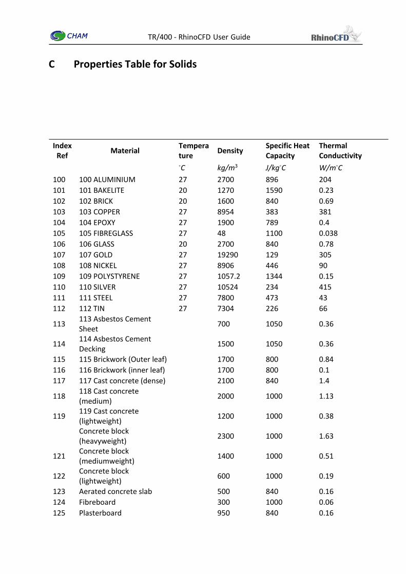
TR/400 - RhinoCFD User Guide
C Properties Table for Solids
Index Ref
Material Temperature
Density Specific Heat Capacity
Thermal Conductivity
◦C kg/m3 J/kg◦C W/m◦C
100 100 ALUMINIUM 27 2700 896 204
101 101 BAKELITE 20 1270 1590 0.23
102 102 BRICK 20 1600 840 0.69
103 103 COPPER 27 8954 383 381
104 104 EPOXY 27 1900 789 0.4
105 105 FIBREGLASS 27 48 1100 0.038
106 106 GLASS 20 2700 840 0.78
107 107 GOLD 27 19290 129 305
108 108 NICKEL 27 8906 446 90
109 109 POLYSTYRENE 27 1057.2 1344 0.15
110 110 SILVER 27 10524 234 415
111 111 STEEL 27 7800 473 43
112 112 TIN 27 7304 226 66
113 113 Asbestos Cement Sheet
700 1050 0.36
114 114 Asbestos Cement Decking
1500 1050 0.36
115 115 Brickwork (Outer leaf) 1700 800 0.84
116 116 Brickwork (inner leaf) 1700 800 0.1
117 117 Cast concrete (dense) 2100 840 1.4
118 118 Cast concrete (medium)
2000 1000 1.13
119 119 Cast concrete (lightweight)
1200 1000 0.38
Concrete block (heavyweight)
2300 1000 1.63
121 Concrete block (mediumweight)
1400 1000 0.51
122 Concrete block (lightweight)
600 1000 0.19
123 Aerated concrete slab 500 840 0.16
124 Fibreboard 300 1000 0.06
125 Plasterboard 950 840 0.16

TR/400 - RhinoCFD User Guide
126 Tile hanging/Roof tile 1900 800 0.84
127 External rendering / Plaster (dense)
1300 1000 0.5
128 Plaster (lightweight) 600 1000 0.16
129 Asphalt/Felt/Bitumen layers
1700 1000 0.5
130 Screed 1200 840 0.41
131 Stone chippings 1800 1000 0.96
132 Wood wool slab 500 1000 0.1
133 Timber flooring / Wood 650 1200 0.14
134 Expanded polystyrene slab 25 1400 0.035
135 Glass fibre slab 12 840 0.04
136 Glass fibre quilt 25 1000 0.035
137 Mineral fibre slab 30 1000 0.035
138 Phenolic foam 30 1400 0.04
139 Polyurethane Board 30 1400 0.025
140 Urea formaldehyde foam 10 1400 0.04
Concentration
Heat And
Momentum
Limited (CHAM)
40 High Street, Wimbledon Village,
London SW19 5AU, UK
Tel: +44 (0)20 947 7651
Web: www.cham.co.uk
Email: [email protected]