Embed Size (px)
Citation preview

USE OF STREAM RESPONSE FUNCTIONS AND STELLA SOFTWARE TO DETERMINE
IMPACTS OF REPLACING SURFACE WATER DIVERSIONS WITH GROUNDWATER
PUMPING WITHDRAWALS ON INSTREAM FLOWS WITHIN THE BERTRAND CREEK
AND FISHTRAP CREEK WATERSHEDS, WASHINGTON STATE, USA
By
ERIK BRIAN PRUNEDA
A dissertation/thesis submitted in partial fulfillment of the requirements for the degree of
MASTER OF SCIENCE IN CIVIL ENGINEERING
WASHINGTON STATE UNIVERSITY Department of Civil and Environmental Engineering
DECEMBER 2007

ii

ACKNOWLEDGMENTS
This research was in part funded by the Department of Public Works, Whatcom County,
Washington, USA. I would like to thank Dr. Diana Allen for allowing the use of the numerical
groundwater model as well as her assistance as a committee member. Thanks to Colette
McKenzie for her research on the streambed hydraulic conductivities of Bertrand and Fishtrap
Creeks. Thanks to Henry Bierlink and Karen Steensma for their knowledge on the study area and
assistance in gaining land access, as well as all landowners who permitted access to their land for
this research. Thanks to Sam Stoner and Brent Collins for assisting in the collection of field data
and Erin Moilanen for her assistance in developing the visual analysis tool. Finally, thanks to the
remaining committee members: Dr. Michael Barber, Dr. Joan Wu, and Dr. Akram Hossain.
iii

USE OF STREAM RESPONSE FUNCTIONS AND STELLA SOFTWARE TO DETERMINE
IMPACTS OF REPLACING SURFACE WATER DIVERSIONS WITH GROUNDWATER
PUMPING WITHDRAWALS ON INSTREAM FLOWS WITHIN THE BERTRAND CREEK
AND FISHTRAP CREEK WATERSHEDS, WASHINGTON STATE, USA
Abstract
by Erik Brian Pruneda, M.S. Washington State University
December 2007
Chair: Michael E. Barber
A numerical groundwater model was used to study the impacts of replacing surface water
diversions with groundwater pumping wells within the Bertrand and Fishtrap watersheds,
Whatcom County, Washington, USA. A regional steady-state groundwater flow model was
calibrated to locally-observed conditions, using stream flow measurements, groundwater level
data, and streambed hydraulic conductivity collected as part of this study. Stream response
functions were calculated for individual wells placed at varying distances from the streams, to
determine the impact these replacement wells might have on the instream flows of Bertrand and
Fishtrap Creeks. Response ratios ranged from 0 to 1.0, with high ratios occurring in close
proximity to the creeks and within areas of high aquifer hydraulic conductivity. Response ratios
less than 1.0 indicate that groundwater pumping wells will have less of an impact on stream flow
than taking the same amount of water directly from a surface water diversion. On the basis of
this modeling study, replacing surface water diversions with groundwater pumping withdrawals
may be a viable alternative for increasing summer stream flows.
iv

TABLE OF CONTENTS
ACKNOWLEDGMENTS........................................................................................................................................ III ABSTRACT .............................................................................................................................................................. IV LIST OF TABLES.................................................................................................................................................... VI LIST OF FIGURES.................................................................................................................................................VII 1. INTRODUCTION ...................................................................................................................................................1 2. PREVIOUS STUDIES ............................................................................................................................................4 3. FIELD INVESTIGATION .....................................................................................................................................8 4. GROUNDWATER FLOW MODEL ...................................................................................................................16
4.1. MODEL BOUNDARY CONDITIONS .....................................................................................................................16 4.1.1 River Boundary Condition ........................................................................................................................16 4.1.2. Specified-Head Boundary ........................................................................................................................22 4.1.3. Drains ......................................................................................................................................................22 4.1.4. Pumping Wells .........................................................................................................................................23 4.1.5. Recharge ..................................................................................................................................................24 4.1.6. Observation Wells ....................................................................................................................................25 4.1.7. Zone Budget .............................................................................................................................................25
4.2. LOCAL MODEL CALIBRATION...........................................................................................................................27 4.2. PROCEDURE FOR DETERMINING IMPACT ON STREAMS DUE TO GROUNDWATER PUMPING...............................30
5. RESULTS...............................................................................................................................................................34 5.1 GROUNDWATER LEVEL AND CLIMATE...............................................................................................................34 5.2 RESPONSE FUNCTIONS .......................................................................................................................................36
6. CONCLUSIONS....................................................................................................................................................42 7. REFERENCES ......................................................................................................................................................45 APPENDIX A.............................................................................................................................................................49 APPENDIX B.............................................................................................................................................................58 APPENDIX C.............................................................................................................................................................62 APPENDIX D.............................................................................................................................................................66
v

LIST OF TABLES
TABLE 1. ESTIMATED DISCHARGE FOR BERTRAND CREEK...........................................................................................10 TABLE 2. ESTIMATED DISCHARGE FOR FISHTRAP CREEK.............................................................................................10 TABLE 3. STREAMBED HYDRAULIC CONDUCTIVITY VALUES USED IN THE GROUNDWATER MODEL. SITE
NAMES CORRESPOND TO FIGURE 7. .....................................................................................................................15 TABLE 4. CONDUCTANCE VALUES FOR EACH RIVER SECTION. .....................................................................................21 TABLE 5. RIVER HEAD CHANGES FOR EACH RIVER SECTION.........................................................................................22 TABLE 6. ESTIMATED INSTANTANEOUS CROP WATER USE IN WID (WUBBENA ET AL., 2004)........................................24 TABLE 7. MONTHLY FACTORS APPLIED TO ALL WATER-RIGHT WELLS. ........................................................................24 TABLE 8. BERTRAND AND FISHTRAP CREEK FLOW RESPONSES, RESPECTIVELY, AS THE PERCENT AREA OF
THEIR CORRESPONDING WATERSHED. .................................................................................................................40 TABLE 9. BERTRAND AND FISHTRAP CREEK COMBINED FLOW RESPONSE AS THE PERCENT AREA OF THEIR
CORRESPONDING WATERSHED.............................................................................................................................41 TABLE 10. BERTRAND AND FISHTRAP CREEK COMBINED FLOW RESPONSE AS THE PERCENT AREA WITHIN 0.5
AND 1.0 MILES OF BERTRAND CREEK..................................................................................................................41 TABLE 11. BERTRAND AND FISHTRAP CREEK COMBINED FLOW RESPONSE AS THE PERCENT AREA WITHIN 0.5
AND 1.0 MILES OF FISHTRAP CREEK....................................................................................................................42
vi

LIST OF FIGURES
FIGURE 1. LOCATION OF LYNDEN, WASHINGTON WITH OUTLINES OF BERTRAND AND FISHTRAP WATERSHEDS. .......................................................................................................................................................3
FIGURE 2. HYDRAULIC CONDUCTIVITY ZONES FOR MODEL LAYER 1 WITHIN THE STUDY AREA. UNITS ARE IN METERS/DAY. ........................................................................................................................................................7
FIGURE 3. HORIZONTAL EXTENT OF THE MODEL DOMAIN, WHITE LINE, AND BOUNDARY OF ABBOTSFORD-SUMAS AQUIFER, RED LINE (SCIBEK AND ALLEN, 2005).......................................................................................8
FIGURE 4. LOCATION OF FLOW MEASUREMENTS. ........................................................................................................11 FIGURE 5. GAINING AND LOSING REACHES AS MEASURED IN JULY 2006 LABELED WITH THE AMOUNT GAINED
FROM OR LOST TO THE AQUIFER IN CUBIC FEET PER SECOND (CFS). .....................................................................12 FIGURE 6. CORRECTED GAINING AND LOSING REACHES FOR JULY 2006 LABELED WITH THE AMOUNT GAINED
FROM OR LOST TO THE AQUIFER IN CUBIC FEET PER SECOND (CFS). .....................................................................13 FIGURE 7. LOCATION OF INSTREAM SLUG TESTS..........................................................................................................14 FIGURE 8. LOCATION OF GROUNDWATER AND SURFACE WATER MONITORING SITES. ..................................................15 FIGURE 9. FOUR SCENARIOS OF STREAM-AQUIFER INTERACTION (DINGMAN, 2002). (A) GAINING STREAM
CONNECTED TO THE AQUIFER. (B) LOSING STREAM CONNECTED TO THE AQUIFER. (C) LOSING STREAM PERCHED ABOVE THE AQUIFER. (D). GAINING AND LOSING STREAM CONNECTED TO THE AQUIFER....................17
FIGURE 10. MODIFIED REPRESENTATION OF A GAINING RIVER REACH WITHIN A MODFLOW CELL (RUMBAUGH ET AL., 1996). .................................................................................................................................19
FIGURE 11. MODIFIED REPRESENTATION OF A LOSING RIVER REACH WITHIN A MODFLOW CELL (RUMBAUGH ET AL., 1996). .................................................................................................................................19
FIGURE 12. START AND END LOCATIONS OF RIVER SECTIONS WITH UNIQUE CONDUCTANCE VALUES. .........................21 FIGURE 13. LOCATION OF COLOR-CODED ZONE BUDGET ZONES. 20 IN TOTAL. ............................................................26 FIGURE 14. VISUAL MODFLOW 4.2 OUTPUT OF MEASURED TO OBSERVED STATIC WATER LEVELS AND
STATISTICS FOR THE ENTIRE MODEL DOMAIN. .....................................................................................................27 FIGURE 15. A COMPARISON OF CORRECTED AND MODELED STREAM FLOWS FOR BERTRAND CREEK. .........................29 FIGURE 16. A COMPARISON OF MEASURED AND MODELED STREAM FLOWS FOR FISHTRAP CREEK. .............................30 FIGURE 17. MODELED WELL LOCATIONS FOR DETERMINATION OF RESPONSE RATIOS. ................................................32 FIGURE 18. WATER-TABLE ELEVATION FOR BERTRAND OBSERVATION WELL # 1 AND LOCAL CUMULATIVE
PRECIPITATION (WAWN, 2007 AND NCDC, 2007B). .........................................................................................35 FIGURE 19. WATER-TABLE ELEVATION FOR BERTRAND OBSERVATION WELL # 1 AND BERTRAND CREEK
WATER DEPTH. ....................................................................................................................................................36 FIGURE 20. RASTER MAP OF BERTRAND CREEK RESPONSE RATIOS. ............................................................................38 FIGURE 21. RASTER MAP OF FISHTRAP CREEK RESPONSE RATIOS. ..............................................................................39 FIGURE 22. COMBINED RASTER INTERPOLATION OF BERTRAND AND FISHTRAP CREEK RESPONSE RATIOS
USING A NATURAL NEIGHBOR TECHNIQUE...........................................................................................................39 FIGURE 23. HYDRAULIC CONDUCTIVITY ZONES FOR MODEL LAYER 3. UNITS ARE IN METERS/DAY. ............................40
vii

1. Introduction
Consumption of water for municipal and irrigation uses can have adverse impacts on minimum
instream flows necessary for ecosystem health. In the Pacific Northwest, this problem is most
acute during summer and early fall months when dry weather and increased demands combine to
create severe water shortages in many streams (Adelsman, 2003). Moreover, the problem is not
just limited to surface water diversions, as many alluvial well withdrawals cause significant
decreases in streams flows through surface and groundwater interaction (Winter et al., 1998).
Recent instream flow studies on two watersheds in Northwest Washington (Bertrand and
Fishtrap) have indicated that summer flows are too low to support desired salmon uses
(Kemblowski et al., 2002; WAC 173-501-030, 1985). An innovative way to manage water
demand is needed to help alleviate this problem. One proposed alternative involves replacing
surface water diversions with groundwater pumping withdrawals. The desire is to have the lag
between the time of groundwater withdrawal and its adverse effect on the stream extend into the
winter rainy season when runoff has begun to increase stream flow and recharge has begun to
replenish the aquifer. While removing surface water diversions will keep the previously-diverted
water in the stream, the overall net effect on stream flow will depend on the location of
replacement wells and the complex interaction of aquifer and streambed properties.
A regional steady-state MODFLOW groundwater model was previously developed by Scibek
and Allen (2005) for use in two studies of the Abbotsford-Sumas Aquifer: to identify the
potential impacts of climate change on groundwater (Scibek and Allen, 2006) and to simulate
nitrate transport within the aquifer (Allen et al., 2007). However, because of the regional scale,
the model contained insufficient localized information to accurately examine groundwater and
surface water interactions for specific stream reaches. The objective of this project was to
1

incorporate local information into the Scibek and Allen groundwater model to determine the
impact on stream flow in Bertrand and Fishtrap Creeks by the exchange of surface water
diversions for groundwater pumping wells. The model was adapted in this study using seepage
analyses data from Bertrand and Fishtrap Creeks, local groundwater and surface water
elevations, streambed hydraulic conductivities, and additional groundwater pumping well
locations and rates of extraction. Because MODFLOW can be difficult to understand and operate
for non-specialists, the simulated stream response functions were incorporated into a
groundwater and surface water interaction tool. The interaction tool was created in the Stella
environment, and allows the user to simulate the effects on the instream flows of Bertrand and
Fishtrap Creeks through exchanging a surface water diversion for a single replacement
groundwater well of the same withdrawal rate, without the need to run the MODFLOW
groundwater model. Because a steady-state groundwater model was used, the stream flow
responses represent a worst-case scenario because the zones of influence of the pumping wells
are at a maximum under steady-state conditions.
The project site is situated within the Abbotsford-Sumas, trans-national aquifer, which extends
from southern British Columbia, Canada southward into northern Washington, USA (Figure 3).
The study area specifically encompasses the Bertrand and Fishtrap watersheds within Whatcom
County near Lynden, Washington (Figure 1). Approximately 46% of the Bertrand watershed,
50.2 km2 (19.4 mi2), and 39% of the Fishtrap watershed, 37.3 km2 (14.4 mi2), are within the
United States, with the remaining areas extending into Canada. Pepin Creek also begins in
Canada and is a significant contributor of water to Fishtrap Creek year around. Bertrand Creek is
a naturally-formed meandering stream, whereas Fishtrap Creek has been channelized in many
places to accommodate agriculture and reduce flooding. The predominant land use within the
2

U.S. for both watersheds is agricultural, with the town of Lynden (population 9,020) being the
only urbanized area in the region. The area has warm, dry summers and mild, wet winters,
receiving on average 88.9 cm (35 in) of precipitation per year, with 18% falling during the
months of June through September, and 82% during the months of October through May
(McKenzie, 2007). The Abbotsford-Sumas Aquifer underlies the study area and is composed
primarily of non-stratified silts, clays, sands, and gravels (Culhane, 1993). The vertical extent of
the aquifer ranges from 7.6 m (25 ft) thick near Blaine, WA (western edge) and 22.8 m (75 ft)
thick near Sumas, WA (eastern edge), while the tertiary bedrock surface underneath the study
area is approximately 213.36 m (700 ft) below the ground surface (Scibek and Allen, 2005).
Figure 1. Location of Lynden, Washington with outlines of Bertrand and Fishtrap watersheds.
3
2. Previous Studies
Welch et al. (1996) conducted a pilot low-flow investigation on several small tributaries and
along the main stem of the Nooksack River during the summer of 1995. The purpose of the
investigation was to collect concurrent stream flow, groundwater level, and precipitation data.
Bertrand and Fishtrap Creeks were found to be gaining reaches from the USA-Canada border to
their termini at the Nooksack River, while Pepin Creek was found to be a losing reach. Recorded
groundwater levels correlated well with daily precipitation measurements.
Cox et al. (2005) conducted a groundwater and surface water interaction study for streams in
the lower Nooksack River basin of Whatcom County, Washington. A network of nine in-stream
piezometers was installed in Fishtrap Creek to measure the local vertical hydraulic gradients
between the stream and underlying aquifer. The magnitudes of the vertical hydraulic gradients
were found to be higher during the winter rain season, November to April, and were lower
during the summer and early fall dry season, June to September. Vertical hydraulic gradients
were generally upward during their study period indicating discharging groundwater, except for
one piezometer located within the town of Lynden. The gradient measurements at this well were
consistently negative indicating stream flow recharging groundwater (Cox et al., 2005). Upon
analyzing individual storm events, Cox et al. (2005) stated that, “surface-water and ground-water
levels respond rapidly to precipitation events, and periods of negative vertical hydraulic
gradients occur during peak streamflows, but typically are of short duration.”
Culhane (1993) calculated theoretical stream depletion rates expected under various pumping
scenarios within the Abbotsford-Sumas Aquifer. The Jenkins analytical model (Jenkins, 1968a,
1968b) was used to calculate the rate of stream depletion caused by nearby wells during and after
pumping. The main assumptions of the Jenkins analytical model are: an isotropic and
4

homogeneous aquifer, a pumping well that is open to the full saturated thickness of the aquifer,
transmissivity does not change with time, and the pumping rate is steady for the entire pumping
period (Jenkins, 1968b). Transmissivity data were estimated for the aquifer from well specific
capacity data. Pumping rates and durations were used in various combinations for this analysis.
While the goal of the study was to determine a critical distance for separating wells from nearby
streams in order to minimize stream depletion, a single critical distance was not found to be
scientifically defensible due to the limitations of the Jenkins model and the variety of factors that
cause stream depletion by pumping wells. The assumptions of the Jenkins model do not hold true
for the Abbotsford-Sumas Aquifer. The aquifer is not isotropic and homogeneous, pumping
wells are not commonly open to the full saturated thickness nor are they pumped continuously at
a steady rate, and because the aquifer is unconfined the transmissivity changes over time.
Analytical models can only provide a rough estimate of stream depletion, whereas a properly
developed numerical model can provide a much more accurate prediction.
A regional groundwater flow model was previously created for the Abbotsford-Sumas Aquifer
using Visual MODFLOW 4.2 by Scibek and Allen (2005). The model was calibrated to steady-
state conditions representative of average August conditions (i.e., stream base flow, groundwater
levels). The lithostratigraphy for the region was mapped using over 2000 well lithologic logs in
combination with surficial geology maps and depositional models. Hydrostratigraphic units were
defined based on the lithostratigraphy and available estimates of hydraulic properties, and the
various units were assigned representative hydraulic conductivity, porosity, and storativity values
(Scibek and Allen, 2005). Ten layers were used to represent the aquifer; each of which was
comprised of varying hydraulic conductivity zones. Hydraulic conductivity zones within the
study area for layer 1 are shown in Figure 2. Additional layers can be found in Appendix C.
5

Model boundary conditions were based on both physical and hydrologic features. The lower
model boundary corresponds to the bedrock surface, as the bedrock is considered relatively
impermeable. The model domain extends slightly beyond the Abbotsford-Sumas aquifer proper,
as illustrated in Figure 3, in order to adequately represent the physical and hydrologic features
that can serve as appropriate model boundary conditions. These include regional surface water
divides to the west and north, and bedrock outcrops to the east. Surface water divides are thought
to approximate the regional groundwater divides as the aquifer is largely unconfined. Other
model boundary conditions include water bodies with specified heads and ditches, corresponding
to the major rivers that receive this drainage (i.e., the Nooksack and the Sumas Rivers), and the
numerous streams that drain the aquifer, respectively. Head values for specified head features
were determined using a combination of survey data and topographic information as described
by Scibek and Allen (2005). Finally, recharge was modeled using the HELP software developed
by the US Environmental Protection Agency, and mapped spatially across the aquifer, taking
into consideration the range of soil media types, shallow aquifer permeability and depth to water-
table (Scibek and Allen, 2006).
In collaboration with Simon Fraser University, I used this model in this study to examine the
complex interactions between the surface water and groundwater in the Bertrand Creek and
Fishtrap Creek watersheds. However, to accomplish the objectives, additional local information
would be needed.
6

Figure 2. Hydraulic conductivity zones for model layer 1 within the study area. Units are in m/d.
7

Figure 3. Horizontal extent of the model domain, white line, and boundary of Abbotsford-Sumas Aquifer, red line (Scibek and Allen, 2005).
3. Field Investigation
The field investigation included seepage analyses of both Bertrand and Fishtrap Creeks and
their tributaries, streambed hydraulic conductivity measurements for both Bertrand and Fishtrap
Creeks, monitoring of static groundwater levels in selected wells near each stream, and
monitoring of stages of each stream.
The seepage analyses were conducted in July 2006 during low-flow conditions. Measurements
were taken using a Pygmy or AA current meter following standard USGS procedures (Buchanan
and Somers, 1969). Velocity and area data for each location were input into a spreadsheet for
discharge estimation (Thomas Cichosz, State of Washington Water Research Center, 2007,
personal communication). According to the Oregon Water Resources Department, the accuracy
of a stream flow measurement is considered to be good if the value is within ±10% of the true
8
stream flow. The locations of flow measurements are shown in Figure 4 and data in Tables 1 and
2.
Bertrand Creek was found to be gaining water from the aquifer up to site B-4 where
presumably, surface water diversions used for irrigation purposes cause the stream flow to
steadily decline (Figure 5). Fishtrap Creek was also found to be a gaining stream, except for site
F-3, where a loss in discharge relative to site F-2 was found (Figure 5). This loss of water seems
to be consistent with the results of the Cox et al. (2005) study.
Estimation of surface water diversions was necessary in order to compare the field flow values
to the predicted values by the MODFLOW Zone Budget analysis within the numerical
groundwater model. Location and quantities of surface water rights were available in the form of
a GIS database created by the Public Utilities District 1 Water Rights Team for the Water
Resource Inventory Area (WRIA) 1 Watershed Management Project. These data were used in
conjunction with local knowledge from Henry Bierlink, Administrator of the Bertrand Watershed
Improvement District, and observations during the field investigation, to determine locations and
quantities of surface water diversions for Bertrand and Fishtrap Creeks. These estimates were
added to the measured field values to obtain “corrected” flows for Bertrand Creek only (Table 1).
Observation during field work as well as analysis of the water right database suggest that
minimal surface diversions are in use for Fishtrap Creek and, as a result, flow values were
unchanged from the field measurements. Upon accounting for the surface water diversions in
Bertrand Creek, virtually all locations were found to be gaining water from the aquifer (Figure
6).
9

Table 1. Estimated discharge for Bertrand Creek.
July 25–26, 2006 Calculated Discharge Data
Site Description Approximate
River Mile
MeasuredDischarge
(cfs)
Estimated Surface Water Withdrawals
(cfs)
Corrected Discharge
(cfs) (B–1) Bertrand Creek on Carlsen Property 8.61 0.8 0.00 0.8 (B–2) Bertrand Creek on Steensma Property 6.74 0.8 0.61 1.4 (B–3) Bertrand Creek at Berthusen Park 5.10 2.5 0.39 3.5 (B–4) Bertrand Creek at Loomis Trail Rd. 4.06 4.3 0.00 5.3 (B–5) Bertrand Creek upstream of Mcklelland Creek 3.17 3.2 0.83 5.1
(B–D1) McClelland Creek – 0.1 0.93 1.0
(B–6) Bertrand Creek south of West Branch 1.82 1.4 3.31 7.4 (B–7) Bertrand Creek at Rathbone Rd. 1.03 0.4 1.50 8.0 (B–8) Bertrand Creek South of Rathbone Rd. 0.62 0.7 0.13 8.4
Table 2. Estimated discharge for Fishtrap Creek.
July 20–21, 2006 Calculated Discharge Data
Site Description Approximate
River Mile
Measured Discharge
(cfs) (F–1) Fishtrap Creek at Assink Rd. 7.45 4.3 (F–2) Fishtrap Creek at Badger Rd. 6.27 4.9 (F–3) Fishtrap Creek at REC Park on Bender Rd. 5.34 3.9 (F–D1) Bender Ditch – 0.5 (F–4) Fishtrap Creek at Lynden Park on Depot Rd. 4.68 5.0 (F–D2) Depot Ditch – 0.3 (F–5) Fishtrap Creek upstream of Double Ditch 3.32 6.4 (F–D3) Pepin Creek upstream of Fishtrap Creek – 1.3 (F–6) Fishtrap Creek at Kok Rd. 2.72 9.8 (F–7) Fishtrap Creek at Flynn Rd. 1.75 9.3 (F–8) Fishtrap Creek at River Rd. 0.23 9.1
10
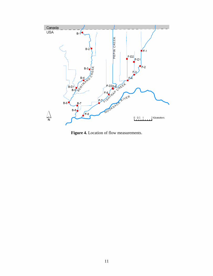
Figure 4. Location of flow measurements.
11
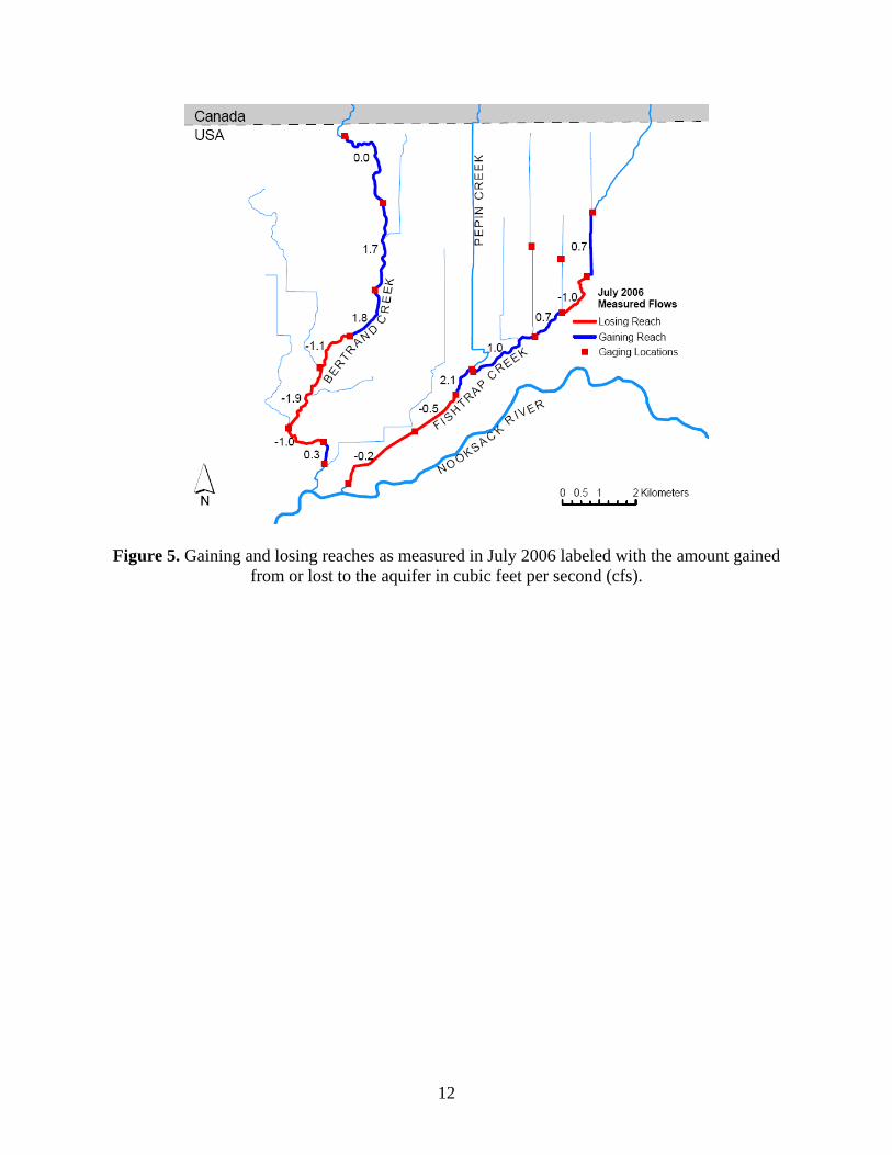
Figure 5. Gaining and losing reaches as measured in July 2006 labeled with the amount gained from or lost to the aquifer in cubic feet per second (cfs).
12

Figure 6. Corrected gaining and losing reaches for July 2006 labeled with the amount gained from or lost to the aquifer in cubic feet per second (cfs).
Instream slug tests were conducted in July 2006 to determine the hydraulic conductivity of the
streambed sediments (Figure 7). Measurements were taken at 0.5 meter and 1.0 meter depths
below the streambed. A full discussion of the instream slug tests and methodology can be found
in McKenzie (2007). The conductivities derived from these tests (Table 3) were used to estimate
the conductance values for the model boundary conditions that are used to represent the streams.
Static groundwater elevations were monitored once every hour by use of Onset Hobo Water
Level Logger pressure transducers and were used to calibrate the groundwater flow model. Six
wells were monitored (Figure 8), each of which was surveyed by Whatcom County to determine
its elevation. All observation wells were not pumped for the duration of the monitoring (July
2006 to July 2007) with the exception of B-3, which was pumped during the summer of 2007.
Plots of the observation well data are provided in Appendix A.
13

Surface water levels in each stream were monitored once every hour using Global Water
pressure transducers and were used in conjunction with the monitored static groundwater
elevations to determine lag times between monitored wells and stream. Two sites were chosen
for installation of the pressure transducers; one in Bertrand Creek and the other in Fishtrap Creek
(Figure 8). Plots of surface water level data are provided in Appendix A.
Figure 7. Location of instream slug tests.
14
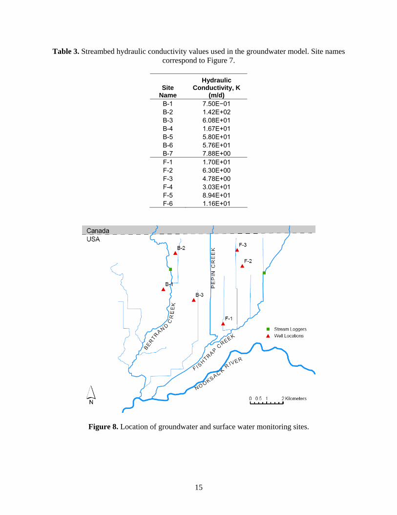
Table 3. Streambed hydraulic conductivity values used in the groundwater model. Site names correspond to Figure 7.
Site Name
Hydraulic Conductivity, K
(m/d) B-1 7.50E−01 B-2 1.42E+02 B-3 6.08E+01 B-4 1.67E+01 B-5 5.80E+01 B-6 5.76E+01 B-7 7.88E+00 F-1 1.70E+01 F-2 6.30E+00 F-3 4.78E+00 F-4 3.03E+01 F-5 8.94E+01 F-6 1.16E+01
Figure 8. Location of groundwater and surface water monitoring sites.
15

4. Groundwater Flow Model
Field measurements of stream flows, recorded groundwater and surface water elevations, and
stream bed hydraulic conductivities, as well as additional groundwater pumping well locations
and rates of extraction were added to the SFU numerical groundwater model or compared to the
Zone Budget results to ensure the best possible local calibration for the Bertrand Creek and
Fishtrap Creek watersheds.
4.1. Model Boundary Conditions
4.1.1 River Boundary Condition
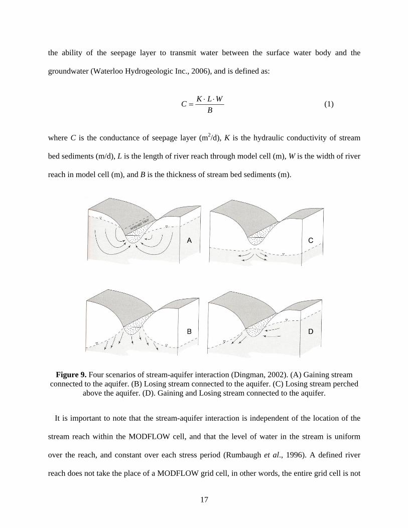
Surface waters may either contribute water to the groundwater system or extract water by
acting as groundwater discharge zones (Figure 9) (Waterloo Hydrogeologic Inc., 2006). The
original SFU model represented all flowing rivers, streams, or creeks as specified-head
boundaries or drains. Specified-head boundaries allow for perfect hydraulic connections between
the surface water and the underlying aquifer, meaning if the head in the aquifer is below that of
the specified-head boundary, a limitless amount of water can be transferred into the groundwater
system. These boundary conditions were used because of the coarse-grained nature of the aquifer
materials and the lack of measured streambed conductivity. However, in order to better simulate
water exchange between the streams and the aquifer and to make use of the available streambed
conductivity data, the boundary conditions for Bertrand, Fishtrap, and Pepin Creeks were
changed to River boundary conditions.
The MODFLOW River package simulates the interaction between groundwater and surface
water via a seepage layer separating the surface water body from the groundwater system
(Waterloo Hydrogeologic Inc., 2006). In addition to providing the surface water elevation, each
cell modeled as a river allows for a conductance term. The conductance of a river cell represents
16
the ability of the seepage layer to transmit water between the surface water body and the
groundwater (Waterloo Hydrogeologic Inc., 2006), and is defined as:
BWLKC ⋅⋅
= (1)
where C is the conductance of seepage layer (m2/d), K is the hydraulic conductivity of stream
bed sediments (m/d), L is the length of river reach through model cell (m), W is the width of river
reach in model cell (m), and B is the thickness of stream bed sediments (m).
Figure 9. Four scenarios of stream-aquifer interaction (Dingman, 2002). (A) Gaining stream connected to the aquifer. (B) Losing stream connected to the aquifer. (C) Losing stream perched
above the aquifer. (D). Gaining and Losing stream connected to the aquifer.
It is important to note that the stream-aquifer interaction is independent of the location of the
stream reach within the MODFLOW cell, and that the level of water in the stream is uniform
over the reach, and constant over each stress period (Rumbaugh et al., 1996). A defined river
reach does not take the place of a MODFLOW grid cell, in other words, the entire grid cell is not
17

given a head value equal to the defined stream elevation. Instead, the river reach is contained
within the MODFLOW grid cell that has a top elevation greater than and bottom elevation less
than the defined bottom elevation of the river’s seepage layer. Figures 10 and 11 demonstrate
gaining and losing river reaches in a MODFLOW grid cell. At the beginning of each
computational iteration, terms representing river seepage are added to the flow equation for each
MODFLOW grid cell containing a river reach (Rumbaugh et al., 1996). Depending on the
elevation of bottom elevation of the seepage layer, either equation (2) or equation (3) is used to
determine the amount of water seepage to or from the river reach (Rumbaugh et al., 1996):
RBOThRBOTHRIVCRIVQRIVRBOThhHRIVCRIVQRIV
<−=>−=
,)(,)(
(2) and (3)
where QRIV is the flow between stream and aquifer (m3/d), CRIV is the hydraulic conductance of
seepage layer (m2/d), HRIV is the head in the stream (m), h is the head in the MODFLOW grid
cell (m), and RBOT is the bottom elevation of the seepage layer (m).
18
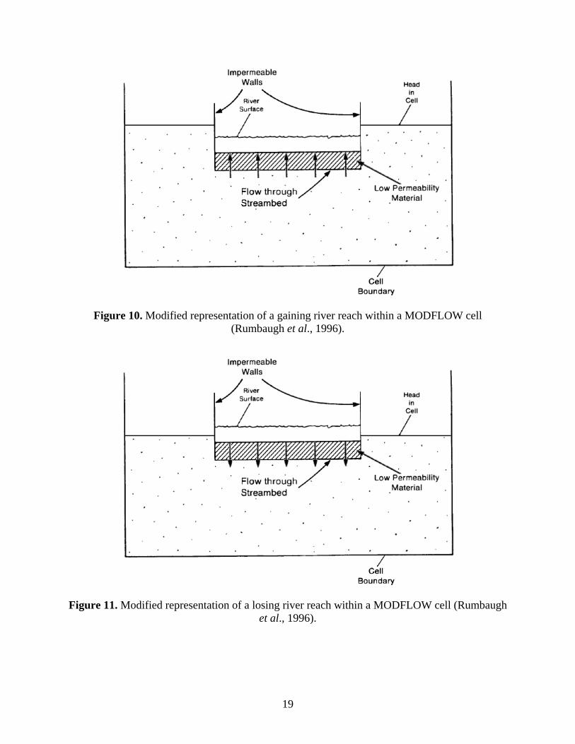
Figure 10. Modified representation of a gaining river reach within a MODFLOW cell (Rumbaugh et al., 1996).
Figure 11. Modified representation of a losing river reach within a MODFLOW cell (Rumbaugh et al., 1996).
19

Each creek was divided into sections: seven in Bertrand Creek, six in Fishtrap Creek, and one
in Pepin Creek (Figure 12). Each section was assigned a conductance value based on the nearest
measurement of streambed hydraulic conductivity (Table 4). All river cells north of the first site
in both Bertrand and Fishtrap Creeks were given the same conductance value as the first river
section in each creek.
The following assumptions were made in the calculation of each conductance term. It was not
feasible to determine the exact river length through each model grid cell. Therefore, the length of
the river through a cell was approximated as the average of the cell height and width for that
section. If a cell was defined with a width of 100 m and a height of 50 m, then the approximated
river length through that cell would have been 75 m. The width of the river through a cell was
assumed to be the same width as measured during the flow measurement nearest each site for the
instream slug test. The thickness of the stream sediments was assumed to be 1.0 m, the
maximum depth of the instream slug tests. A sediment thickness of 0.75 m was assigned if the
calculated hydraulic conductivity of the 0.5 m slug test was lower than that of the 1.0 m slug test.
In addition to surveying the well elevations, Whatcom County created benchmarks on two
bridges in Bertrand Creek and two in Fishtrap Creek. These benchmarks allowed for manual
recording of the surface water elevation throughout the year. To assure that the modeled surface
water elevations for Bertrand and Fishtrap Creeks were representative of August low-flow
conditions, the specified heads originally assigned in the model were compared with the lowest
recorded surveyed surface water elevations. It was found that the original modeled river heads
were too low. The heads were subsequently increased accordingly to match the surveyed values
(Table 5).
20

Figure 12. Start and end locations of river sections with unique conductance values.
Table 4. Conductance values for each river section.
Site Name
Hydraulic Conductivity, K
(m/d)
Stream Width
(m)
Stream Length
(m)
Sediment Thickness
(m) Conductance
(m2/d) B–1 7.50E−01 4.5 75 0.75 3.38E+02 B–2 1.42E+02 3.3 100 1.00 4.70E+04 B–3 6.08E+01 3.7 100 1.00 2.25E+04 B–4 1.67E+01 3.2 100 1.00 5.35E+03 B–5 5.80E+01 3.0 100 0.75 2.32E+04 B–6 5.76E+01 3.0 100 1.00 1.73E+04 B–7 7.88E+00 4.3 100 0.75 4.52E+03 F–1 1.70E+01 5.5 50 1.00 4.66E+03 F–2 6.30E+00 4.3 75 0.75 2.71E+03 F–3 4.78E+00 4.5 75 1.00 1.61E+03 F–4 3.03E+01 6.7 100 1.00 2.03E+04 F–5 8.94E+01 4.8 100 1.00 4.29E+04 F–6 1.16E+01 4.0 100 1.00 4.64E+03 P–1 8.94E+01 2.0 100 1.00 1.79E+04
21
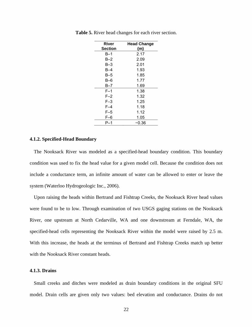
Table 5. River head changes for each river section.
River Section
Head Change (m)
B–1 2.17 B–2 2.09 B–3 2.01 B–4 1.93 B–5 1.85 B–6 1.77 B–7 1.69 F–1 1.38 F–2 1.32 F–3 1.25 F–4 1.18 F–5 1.12 F–6 1.05 P–1 −0.36
4.1.2. Specified-Head Boundary
The Nooksack River was modeled as a specified-head boundary condition. This boundary
condition was used to fix the head value for a given model cell. Because the condition does not
include a conductance term, an infinite amount of water can be allowed to enter or leave the
system (Waterloo Hydrogeologic Inc., 2006).
Upon raising the heads within Bertrand and Fishtrap Creeks, the Nooksack River head values
were found to be to low. Through examination of two USGS gaging stations on the Nooksack
River, one upstream at North Cedarville, WA and one downstream at Ferndale, WA, the
specified-head cells representing the Nooksack River within the model were raised by 2.5 m.
With this increase, the heads at the terminus of Bertrand and Fishtrap Creeks match up better
with the Nooksack River constant heads.
4.1.3. Drains
Small creeks and ditches were modeled as drain boundary conditions in the original SFU
model. Drain cells are given only two values: bed elevation and conductance. Drains do not
22

affect the flow model unless the groundwater table rises above a defined drain elevation. During
the low-flow period for which the steady-state model is based, most drains are not in contact
with the groundwater table because their bed elevations are above the groundwater table under
August conditions. These drains function under transient conditions. Drains surrounding
Bertrand and Fishtrap Creeks were modified from their original conductance values of 100 m2/d
and given values similar to those found in the nearest Bertrand or Fishtrap Creek river section.
4.1.4. Pumping Wells
The original SFU model only included selected pumping wells from the Washington State
Department of Ecology’s well log database. When combined, the wells within the Bertrand
Watershed Improvement District (WID) totaled a pumping rate of 138 liter/s (4.88 cfs).
According to Wubbena et al. (2004), 2995 hectares (7,400 acres) within the Bertrand WID
require approximately 1379 l/s (48.71 cfs) of groundwater during the month of July for irrigation
purposes. In order to properly simulate the local conditions, all groundwater rights, certificates,
and claims were added to the model.
A water right database developed by the Public Utilities District 1 Water Rights Team for the
Water Resource Inventory Area (WRIA) 1 Watershed Management Project was used to import
groundwater rights, certificates, and claims into the groundwater model. Because the amount of
pumping does not generally match the written water right at all times of the year, all water rights
were scaled month-to-month to match the estimated groundwater irrigation use for the Bertrand
Watershed Improvement District as determined by Hydrologic Services Company (Table 6)
(Wubbena et al., 2004). The water rights, certificates, and claims within the Bertrand Watershed
Improvement District were scaled to match those groundwater irrigation use rates for each month
of the year. Those monthly factors (Table 7) were then applied to the remaining water rights,
23

certificates, and claims within the Fishtrap watershed. Pumping rates for the steady-state model
were taken to be those of July, the month with the greatest pumping rates.
Table 6. Estimated instantaneous crop water use in WID (Wubbena et al., 2004).
Surface Water Irrigation Use
(cfs)
Ground Water Irrigation Use
(cfs)
Total Irrigation Use
(cfs) Month Sprinkler Drip Total Sprinkler Drip Total Sprinkler Drip Total
Jan 0.00 0.00 0.00 0.00 0.00 0.00 0.00 0.00 0.00Feb 0.00 0.00 0.00 0.00 0.00 0.00 0.00 0.00 0.00Mar 0.00 0.00 0.00 0.10 0.00 0.10 0.10 0.00 0.10Apr 0.07 0.00 0.07 4.67 0.00 4.67 4.74 0.00 4.74May 0.51 2.46 2.97 16.54 2.55 19.09 17.05 5.01 22.06Jun 0.83 4.36 5.19 23.65 4.52 28.17 24.48 8.88 33.36Jul 1.60 6.10 7.70 42.38 6.33 48.71 43.98 12.43 56.41Aug 1.28 3.84 5.12 34.50 3.99 38.49 35.78 7.83 43.61Sep 0.34 0.52 0.86 11.66 0.54 12.20 12.00 1.06 13.06Oct 0.00 0.00 0.00 0.00 0.00 0.00 0.00 0.00 0.00Nov 0.00 0.00 0.00 0.00 0.00 0.00 0.00 0.00 0.00Dec 0.00 0.00 0.00 0.00 0.00 0.00 0.00 0.00 0.00
Table 7. Monthly factors applied to all water-right wells.
Month Scaling Factor Jan 0.000 Feb 0.000 Mar 0.001 Apr 0.053 May 0.217 Jun 0.321 Jul 0.554 Aug 0.438 Sep 0.139 Oct 0.000 Nov 0.000 Dec 0.000
4.1.5. Recharge
Recharge rates were defined in the SFU model based on spatial distributions of a number of
factors: type of soil cover, aquifer material, and water-table depth. Average mean annual climate
24
data were used in running the HELP (Hydrologic Evaluation of Landfill Performance, US EPA)
model for one-dimensional soil columns. The resulting recharge results were mapped spatially
and used as input to the groundwater flow model. A full discussion of the recharge mapping and
methodology can be found in Scibek and Allen (2006).
To make sure that average annual recharge values would be acceptable when using 2006 field
data to adapt the model, annual precipitation for 2006 at Clearbrook, WA was compared to the
normal precipitation observed since the year 1919. For 2006 a total of 113.9 cm (44.86 inches) of
rain was recorded, which amounted to only 2.3 cm (0.91 inches) less than normal (NCDC,
2007a). This departure from normal was not significant enough to warrant a reduction of the
recharge values previously defined by Scibek and Allen.
4.1.6. Observation Wells
In addition to the more than 1000 existing observation wells input in the model by SFU, the six
observation wells described previously in section 3, along with a number of USGS wells
(Appendix B), were added to the groundwater model to ensure that the model correctly predicted
the water-table elevations.
4.1.7. Zone Budget
Within MODFLOW, Zone Budget was used to calculate sub-regional water budgets for
specific sections of Bertrand and Fishtrap Creeks, along with Pepin Creek and other major
drains. For each sub-regional water budget (zone), the cell by cell budget results produced by
MODFLOW are tabulated by Zone Budget (Waterloo Hydrogeologic Inc., 2006). A total of 20
zones were created between locations of measured stream flow; eight in Bertrand Creek, eight in
Fishtrap Creek, one in Pepin Creek, and three for major drains (Figure 13). Only cells that were
25

defined as river or drain boundaries were included in a zone. Beginning with known flows from
Environment Canada gaging stations at the USA-Canada border for Bertrand, Fishtrap, and
Pepin Creeks, the predicted gains and losses from each river reach or zone were added to or
subtracted from the known flow and compared to our measured flow values to determine the
accuracy or validity of the model. The stream routing package within Visual MODFLOW would
have accounted for the flows automatically, but the river package was chosen in order to
preserve the original surface water head values developed by SFU.
Figure 13. Location of color-coded zone budget zones. 20 in total.
26

4.2. Local Model Calibration
Throughout the entire model domain, the calibration of observed to measured static water
levels (Figure 14) yielded a Root Mean Squared (RMS) error of 10.0 m, with a normalized RMS
error of 8.7% and a residual mean error of 3.5 m. The calibration statistics were found to be
similar to those of the original model developed by Scibek and Allen (2005), which were
regarded to be reasonable given the scale of the model and the number of observations (Scibek
and Allen, 2005).
Figure 14. Visual MODFLOW 4.2 output of measured to observed static water levels and statistics for the entire model domain.
27

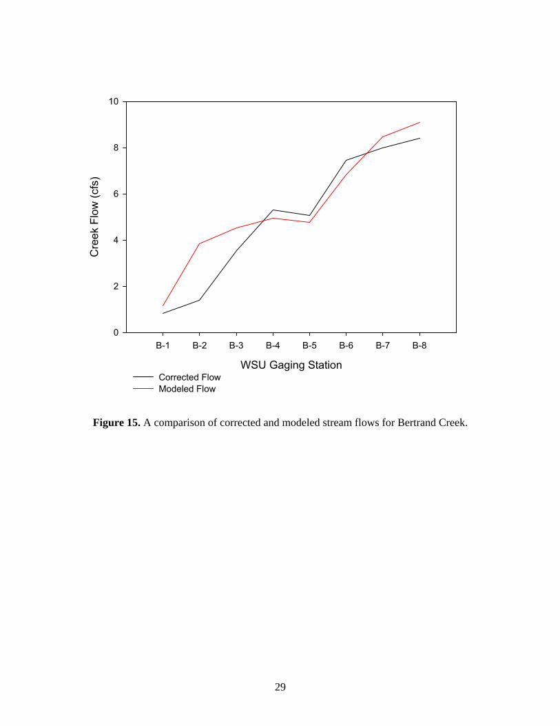
Locally the calibration results point to some discrepancies between “corrected” and modeled
stream flows. A comparison of the “corrected” creek flows and modeled flows for Bertrand
Creek (Figure 15) and measured flows and modeled flows for Fishtrap Creek (Figure 16)
revealed that the model over-predicted the stream flow in the area of station B-2, and slightly
over-predicted stream flow in the upper reaches of Fishtrap Creek; however, the model closely
matched the “corrected” flows in the lower reaches of Bertrand Creek and the measured flows of
Fishtrap Creek. The overestimation of river leakage in the upper reaches of both creeks may be
due to non-permitted wells which are unaccounted for, uncertainty in stream elevations, or the
hydraulic conductivity of the aquifer materials may be to low within those areas. A comparison
of the observed heads and the modeled heads within the study area yielded better statistics than
the overall model, with a RMS error of 3.1 m, a normalized RMS error of 5.4% and a residual
mean error of 1.8 m.
28
WSU Gaging Station
B-1 B-2 B-3 B-4 B-5 B-6 B-7 B-8
Cre
ek F
low
(cfs
)
0
2
4
6
8
10
Corrected FlowModeled Flow
Figure 15. A comparison of corrected and modeled stream flows for Bertrand Creek.
29

WSU Gaging Station
F-1 F-2 F-3 F-4 F-5 F-6 F-7 F-8
Cre
ek F
low
(cfs
)
3
4
5
6
7
8
9
10
11
Measured FlowModeled Flow
Figure 16. A comparison of measured and modeled stream flows for Fishtrap Creek.
4.2. Procedure for Determining Impact on Streams Due to Groundwater Pumping
Barlow et al. (2003) and Cosgrove and Johnson (2004) created groundwater models using
MODFLOW to study the local groundwater and surface water interactions for the Hunt-
Annaquatucket-Pettaquamscutt stream-aquifer, Rhode Island, and the Snake River Plain, Idaho,
respectively. The goal in both studies was to create stream response functions that would allow
them to quantify the impacts of groundwater pumping on surface water flows.
Using a response-matrix technique, Barlow et al. (2003) coupled a numerical groundwater
model and optimization techniques to maximize total groundwater withdrawal from the Hunt-
30

Annaquatucket-Pettaquamscutt stream-aquifer of central Rhode Island, during the summer
months of July, August and September, while maintaining desired stream flows. Response
functions were generated for 14 public water supply wells and 2 hypothetical wells. Barlow et al.
(2003) assumed the rate of stream flow depletion at a constraint site to be a linear function of the
pumping rate of each groundwater well. By assuming linearity, the concept of superposition
allowed for individual stream flow depletions caused by each well to be summed together at a
constraint site to derive a total stream flow depletion.
Cosgrove and Johnson (2004) modified an existing single layer, unconfined, transient
MODFLOW groundwater model for the Snake River Plain Aquifer, Idaho, for use with the
MODRSP code to generate response functions. The unconfined groundwater model was
converted to a confined system, to conform to the MODRSP requirement of modeling a linear
system. Transient response functions for 51 river cells were generated for each of the numerical
model cells using 150 four-month stress periods representing 50 years. The response functions
are a result of a unit stress applied only during the first stress period and, as a result, they
represent the propagation of the effects of that unit stress over time. Making use of the transient
response functions, a spreadsheet was developed that allows the user to enter water use scenarios
and determine the impact to surface water resources.
For this study, response functions were manually created for each of 346 hypothetical well
locations (Figure 17). Pumping wells were added to the calibrated steady-state groundwater flow
model, one at a time, and the stream flow impacts were recorded for each through the use of
Zone Budget. Each pumping well was given a screen interval of 9–13 m below the ground
surface, and because response functions are typically based on a unit stress, the wells were
assigned a pumping rate of 1 cubic foot per second (cfs) (Cosgrove and Johnson, 2004). For each
31

well location, a response ratio, ranging from 0.0 to 1.0, was determined for Bertrand Creek and
Fishtrap Creek as the change in modeled stream flow at each creek’s terminus with the Nooksack
River divided by the pumping rate. As in Barlow et al. (2003) and Cosgrove and Johnson (2004)
it was assumed that the rate of stream flow depletion at each constraint site is a linear function of
the pumping rate of each groundwater well. Due to the unconfined nature of the groundwater
model, the decline in water level was assumed to be very small such that linearity could be
approximated. Response ratios less than 1.0 indicate that groundwater pumping wells would
have less of an impact on stream flow than taking the same amount of water directly from a
surface water diversion.
Figure 17. Modeled well locations for determination of response ratios.
Raster maps of the response ratios with a 100 m cell size were created for each stream using
natural neighbor interpolation in ArcGIS. Natural neighbor interpolation uses a subset of data
32
points that surround a query point and applies weights to them based on proportionate areas in
order to interpolate a value (Sibson, 1981).
The mapped response zones were used to create a groundwater and surface water interaction
tool, whereby the user can replace a surface water diversion with a groundwater pumping well of
the same withdrawal rate, and determine the stream flow impact to Bertrand and Fishtrap Creeks
at their terminus with the Nooksack River. STELLA version 9.0.3 by isee Systems was chosen as
the modeling environment for the interaction tool. The users can choose between 4 regions of
interest within the study area, and then select one of four sub-regions within that chosen region.
Upon choosing a sub-region, the user can easily locate the location of a surface water diversion,
and determine the best location for a replacement groundwater well. Overlain on the sub-region
maps are the mapped response function zones for Bertrand and Fishtrap Creeks. The user then
identifies the Bertrand Creek response zone and the Fishtrap Creek response zone for which the
desired replacement groundwater well falls, and enters a value for the surface water withdrawal
rate to be replaced by the groundwater well. Using the response functions and the provided user
input, the STELLA model compares the stream flow values for Bertrand and Fishtrap Creeks for
each of a surface water replacement well and a surface water diversion. The impact to each creek
is determined as the difference between those two sets of flow values. The user may, through
trial-and-error, select the best option, but must personally keep track of the stream flow impacts
for each case. The STELLA model is not capable of storing the locations of surface water
diversions or the replacement groundwater pumping wells; it is only capable of determining the
stream flow impacts for a single surface water replacement well. Screen captures of the STELLA
model are shown in Appendix D.
33

A limitation of the approach is that a groundwater flow model was used, rather than a coupled
surface water-groundwater model. As such, the boundary conditions used to represent the
streams are fixed (specified heads). Thus, the impact on stream discharge cannot be simulated,
i.e., while the stream discharge can vary in the simulations, this change in discharge is not
reflected as a shift in stream stage. However, because we are replacing a surface water diversion
for a single groundwater pumping well of the same withdrawal rate, the impact to stream stage is
considered to be minimal.
5. Results
5.1 Groundwater Level and Climate
The recorded groundwater elevations for Bertrand observation well # 1 appear to correlate
with local precipitation events (Figure 18). Hourly precipitation data were acquired from the
Public Agricultural Weather System (PAWS) weather station in Lynden, Washington, and
Bellingham International Airport weather data were used to fill in missing data from the PAWS
weather station. During the summer months, the slope of the cumulative precipitation curve is
small, and during the winter months the slope is large and appears to account for groundwater
elevation changes. Also, there appears to be little lag time between Bertrand observation well # 1
and the nearby upstream Bertrand Creek stream logger (Figure 19). These observations suggest
that the groundwater and surface water are well connected. Additional observation well plots can
be found in Appendix A.
34

Date
8/1/2006 12/1/2006 4/1/2007 8/1/2007
Wat
er T
able
Ele
vatio
n (m
)
31.0
31.5
32.0
32.5
33.0
33.5
34.0
34.5
35.0A
ccumulated P
recipitation (mm
)
0
200
400
600
800
1000
Bertrand Observation Well # 1 Accumulated Precipitation
Figure 18. Water-table elevation for Bertrand observation well # 1 and local cumulative precipitation (WAWN, 2007 and NCDC, 2007b).
35

Date
8/1/2006 12/1/2006 4/1/2007 8/1/2007
Wat
er T
able
Ele
vatio
n (m
)
31.0
31.5
32.0
32.5
33.0
33.5
34.0
34.5
35.0W
ater Depth (m
)
0
1
2
3
Bertrand Observation Well # 1 Bertrand Creek Water Depth
Figure 19. Water-table elevation for Bertrand observation well # 1 and Bertrand Creek water depth.
5.2 Response Functions
Maps of the well response functions for each of Bertrand and Fishtrap Creek are shown in
Figures 20 and 21. Because wells were placed by rows, the areas between the modeled rows are
lacking data and, as a result, the interpolation does not accurately predict stream flow impacts
due to pumping wells within those areas. In future work, more wells should be modeled along
each creek in order to fill gaps of missing response ratio data.
36

Pumping wells placed east of Fishtrap Creek have almost no discernable impact on Bertrand
Creek. Similarly, pumping wells placed west of Bertrand Creek have almost no discernable
impact on Fishtrap Creek. However, groundwater pumping wells located in the area between
Bertrand and Fishtrap Creeks can impact stream flows in both creeks. There are reaches where
groundwater pumping has less of an impact on the stream flow on one side of the creek as
opposed to the other. To better illustrate the overall response functions, a combined response
ratio interpolation map was created by adding the Bertrand Creek and Fishtrap Creek responses
for each well location (Figure 22).
Variations in the spatial distribution of response ratios appear to be correlated with spatial
variations in the hydraulic conductivity within the model layer containing the screened interval
of the pumping well (Figure 23). Surface water replacement wells placed within zones with high
hydraulic conductivity values seem to produce greater responses to the instream flows of
Bertrand and Fishtrap Creeks.
Table 8 presents the Bertrand and Fishtrap Creek flow responses, respectively, as the percent
area of their corresponding watershed. 79% of the Bertrand Creek watershed and 79% of the
Fishtrap Creek watershed have response ratios less than 0.5. However, because groundwater
movement occurs across watershed boundaries, stream flow impacts to Fishtrap Creek can occur
from wells within the Bertrand Creek watershed. A surface water replacement well should not be
allowed to benefit one creek while harming the other. Table 9 presents the combined flow
response for Bertrand and Fishtrap Creeks as the percent area of their corresponding watershed.
67% of the Bertrand Creek watershed and 79% of the Fishtrap Creek watershed have combined
response ratios less than 0.5, indicating very favorable exchange opportunities. However, it
might not be economically practical for farmers to replace their surface water diversion for a
37

groundwater withdrawal if they have to construct a lengthy pipeline in order to get the water to
their field. Consequently, stream flow responses from wells located within narrow bands of both
streams were specifically examined. Of the area within a 0.5 mile band of Bertrand Creek, 57%
has a combined flow response ratio less than 0.5, and within a 1.0 mile band, 64% has a
combined flow response ratio less than 0.5 (Table 10). Of the area within a 0.5 mile band of
Fishtrap Creek, 70% has a combined flow response ratio less than 0.5, and within a 1.0 mile
band, 77% has a combined flow response ratio less than 0.5 (Table 11).
Figure 20. Raster map of Bertrand Creek response ratios.
38

Figure 21. Raster map of Fishtrap Creek response ratios.
Figure 22. Combined raster interpolation of Bertrand and Fishtrap Creek response ratios using a natural neighbor technique.
39
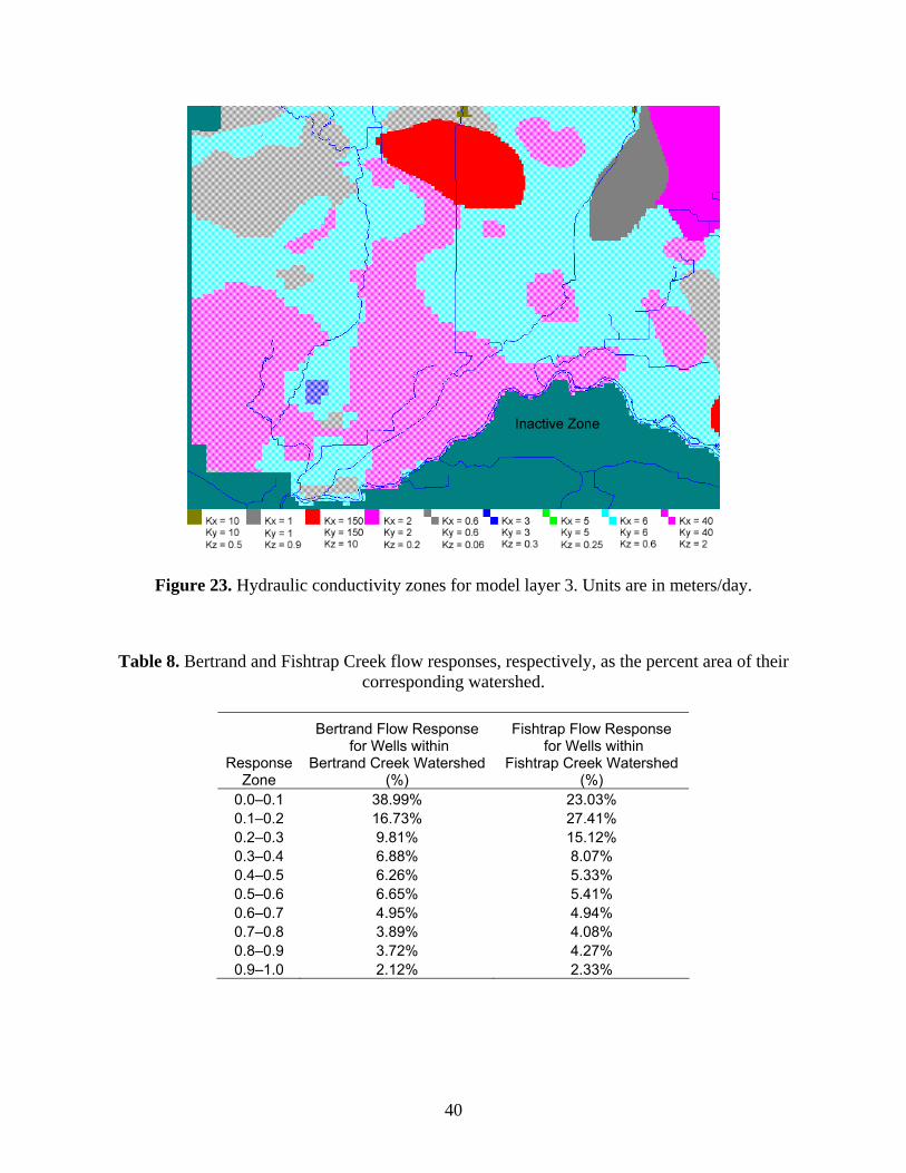
Figure 23. Hydraulic conductivity zones for model layer 3. Units are in meters/day.
Table 8. Bertrand and Fishtrap Creek flow responses, respectively, as the percent area of their corresponding watershed.
Response Zone
Bertrand Flow Response for Wells within
Bertrand Creek Watershed(%)
Fishtrap Flow Response for Wells within
Fishtrap Creek Watershed (%)
0.0–0.1 38.99% 23.03% 0.1–0.2 16.73% 27.41% 0.2–0.3 9.81% 15.12% 0.3–0.4 6.88% 8.07% 0.4–0.5 6.26% 5.33% 0.5–0.6 6.65% 5.41% 0.6–0.7 4.95% 4.94% 0.7–0.8 3.89% 4.08% 0.8–0.9 3.72% 4.27% 0.9–1.0 2.12% 2.33%
40
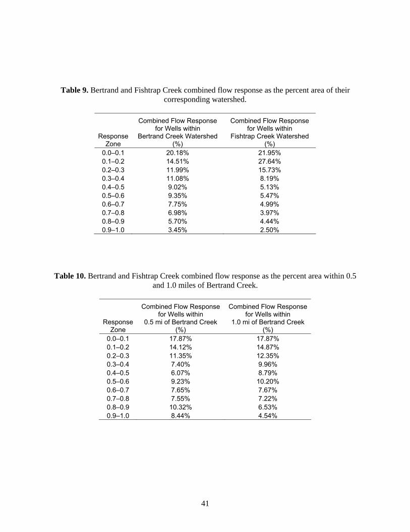
Table 9. Bertrand and Fishtrap Creek combined flow response as the percent area of their corresponding watershed.
Response Zone
Combined Flow Response for Wells within
Bertrand Creek Watershed(%)
Combined Flow Response for Wells within
Fishtrap Creek Watershed (%)
0.0–0.1 20.18% 21.95% 0.1–0.2 14.51% 27.64% 0.2–0.3 11.99% 15.73% 0.3–0.4 11.08% 8.19% 0.4–0.5 9.02% 5.13% 0.5–0.6 9.35% 5.47% 0.6–0.7 7.75% 4.99% 0.7–0.8 6.98% 3.97% 0.8–0.9 5.70% 4.44% 0.9–1.0 3.45% 2.50%
Table 10. Bertrand and Fishtrap Creek combined flow response as the percent area within 0.5 and 1.0 miles of Bertrand Creek.
Response Zone
Combined Flow Responsefor Wells within
0.5 mi of Bertrand Creek (%)
Combined Flow Response for Wells within
1.0 mi of Bertrand Creek (%)
0.0–0.1 17.87% 17.87% 0.1–0.2 14.12% 14.87% 0.2–0.3 11.35% 12.35% 0.3–0.4 7.40% 9.96% 0.4–0.5 6.07% 8.79% 0.5–0.6 9.23% 10.20% 0.6–0.7 7.65% 7.67% 0.7–0.8 7.55% 7.22% 0.8–0.9 10.32% 6.53% 0.9–1.0 8.44% 4.54%
41
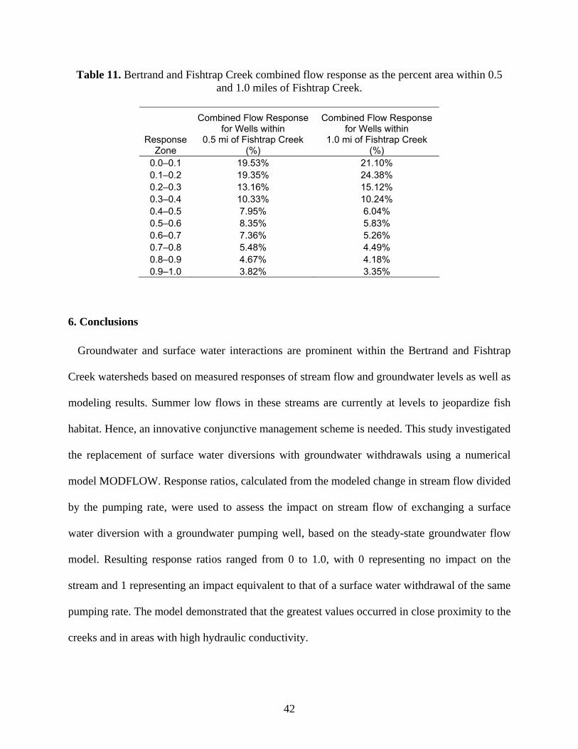
Table 11. Bertrand and Fishtrap Creek combined flow response as the percent area within 0.5 and 1.0 miles of Fishtrap Creek.
Response Zone
Combined Flow Responsefor Wells within
0.5 mi of Fishtrap Creek (%)
Combined Flow Response for Wells within
1.0 mi of Fishtrap Creek (%)
0.0–0.1 19.53% 21.10% 0.1–0.2 19.35% 24.38% 0.2–0.3 13.16% 15.12% 0.3–0.4 10.33% 10.24% 0.4–0.5 7.95% 6.04% 0.5–0.6 8.35% 5.83% 0.6–0.7 7.36% 5.26% 0.7–0.8 5.48% 4.49% 0.8–0.9 4.67% 4.18% 0.9–1.0 3.82% 3.35%
6. Conclusions
Groundwater and surface water interactions are prominent within the Bertrand and Fishtrap
Creek watersheds based on measured responses of stream flow and groundwater levels as well as
modeling results. Summer low flows in these streams are currently at levels to jeopardize fish
habitat. Hence, an innovative conjunctive management scheme is needed. This study investigated
the replacement of surface water diversions with groundwater withdrawals using a numerical
model MODFLOW. Response ratios, calculated from the modeled change in stream flow divided
by the pumping rate, were used to assess the impact on stream flow of exchanging a surface
water diversion with a groundwater pumping well, based on the steady-state groundwater flow
model. Resulting response ratios ranged from 0 to 1.0, with 0 representing no impact on the
stream and 1 representing an impact equivalent to that of a surface water withdrawal of the same
pumping rate. The model demonstrated that the greatest values occurred in close proximity to the
creeks and in areas with high hydraulic conductivity.
42
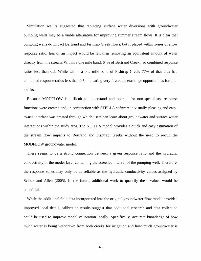
Simulation results suggested that replacing surface water diversions with groundwater
pumping wells may be a viable alternative for improving summer stream flows. It is clear that
pumping wells do impact Bertrand and Fishtrap Creek flows, but if placed within zones of a low
response ratio, less of an impact would be felt than removing an equivalent amount of water
directly from the stream. Within a one mile band, 64% of Bertrand Creek had combined response
ratios less than 0.5. While within a one mile band of Fishtrap Creek, 77% of that area had
combined response ratios less than 0.5, indicating very favorable exchange opportunities for both
creeks.
Because MODFLOW is difficult to understand and operate for non-specialists, response
functions were created and, in conjunction with STELLA software, a visually-pleasing and easy-
to-use interface was created through which users can learn about groundwater and surface water
interactions within the study area. The STELLA model provides a quick and easy estimation of
the stream flow impacts to Bertrand and Fishtrap Creeks without the need to re-run the
MODFLOW groundwater model.
There seems to be a strong connection between a given response ratio and the hydraulic
conductivity of the model layer containing the screened interval of the pumping well. Therefore,
the response zones may only be as reliable as the hydraulic conductivity values assigned by
Scibek and Allen (2005). In the future, additional work to quantify these values would be
beneficial.
While the additional field data incorporated into the original groundwater flow model provided
improved local detail, calibration results suggest that additional research and data collection
could be used to improve model calibration locally. Specifically, accurate knowledge of how
much water is being withdrawn from both creeks for irrigation and how much groundwater is
43

being pumped in the surrounding area is lacking. Knowledge of this information would help to
improve the calibration of the groundwater model. Furthermore, additional well monitoring
stations are needed to observe the groundwater table elevation throughout the year.
Transient effects were also not studied in this project. In order to determine precisely when the
effects of a pumped well will impact a nearby stream, a transient model is needed. The steady-
state model predicted how much the stream will be impacted given an infinite amount of time
and, therefore, represents a worst-case scenario. A transient model can indicate when and by how
much a pumped well will impact a stream assuming sufficient pumping data are available. A
transient version of the groundwater flow model is available from SFU, and if updated according
to this study, could be used to investigate transient conditions.
44
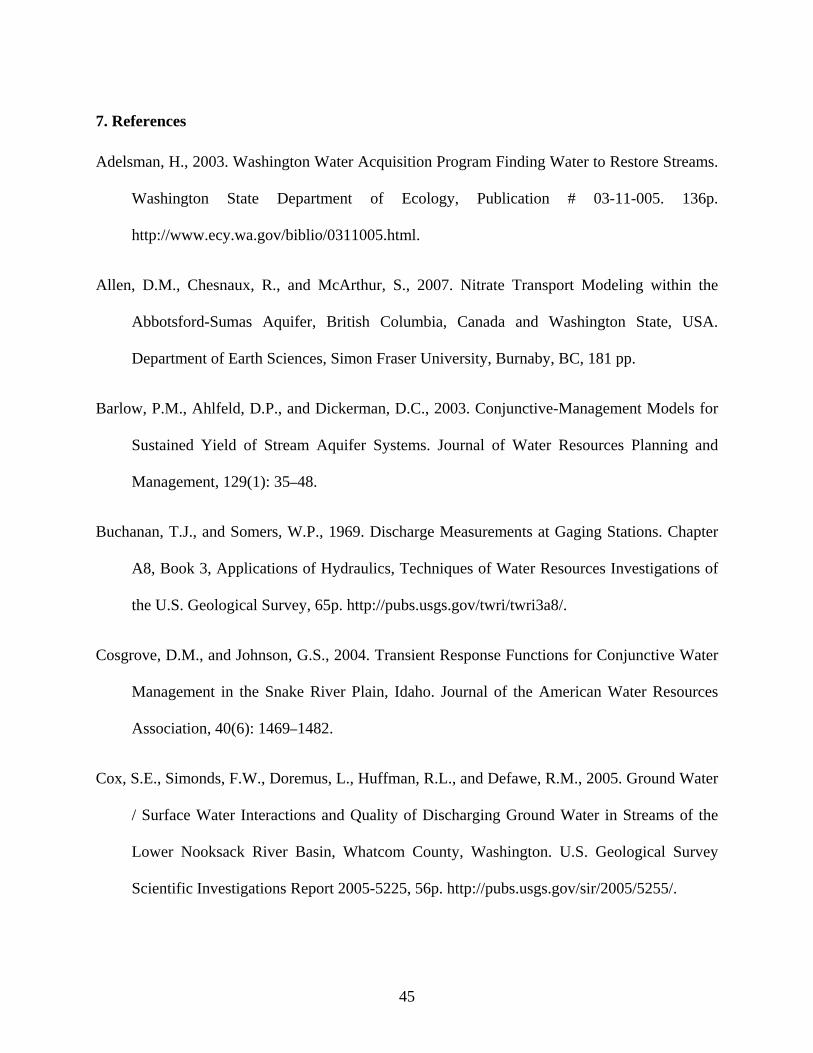
7. References
Adelsman, H., 2003. Washington Water Acquisition Program Finding Water to Restore Streams.
Washington State Department of Ecology, Publication # 03-11-005. 136p.
http://www.ecy.wa.gov/biblio/0311005.html.
Allen, D.M., Chesnaux, R., and McArthur, S., 2007. Nitrate Transport Modeling within the
Abbotsford-Sumas Aquifer, British Columbia, Canada and Washington State, USA.
Department of Earth Sciences, Simon Fraser University, Burnaby, BC, 181 pp.
Barlow, P.M., Ahlfeld, D.P., and Dickerman, D.C., 2003. Conjunctive-Management Models for
Sustained Yield of Stream Aquifer Systems. Journal of Water Resources Planning and
Management, 129(1): 35–48.
Buchanan, T.J., and Somers, W.P., 1969. Discharge Measurements at Gaging Stations. Chapter
A8, Book 3, Applications of Hydraulics, Techniques of Water Resources Investigations of
the U.S. Geological Survey, 65p. http://pubs.usgs.gov/twri/twri3a8/.
Cosgrove, D.M., and Johnson, G.S., 2004. Transient Response Functions for Conjunctive Water
Management in the Snake River Plain, Idaho. Journal of the American Water Resources
Association, 40(6): 1469–1482.
Cox, S.E., Simonds, F.W., Doremus, L., Huffman, R.L., and Defawe, R.M., 2005. Ground Water
/ Surface Water Interactions and Quality of Discharging Ground Water in Streams of the
Lower Nooksack River Basin, Whatcom County, Washington. U.S. Geological Survey
Scientific Investigations Report 2005-5225, 56p. http://pubs.usgs.gov/sir/2005/5255/.
45

Culhane, T., 1993. Whatcom County Hydraulic Continuity Investigation – Part 1, Critical
Well/Stream Separation Distances for Minimizing Stream Depletion. Washington State
Department of Ecology Open File Technical Report 93-08. 20p.
http://www.ecy.wa.gov/biblio/9308.html.
Dingman, S.L., 2002. Physical Hydrology, Second Edition. Prentice Hall, New Jersey.
Jenkins, C.T., 1968a. Techniques for Computing Rate and Volume of Stream Depletion by
Wells. Ground Water, 6(2): 37–46.
Jenkins, C.T., 1968b. Computation of Rate and Volume of Stream Depletion by Wells. Chapter
D1, Book 4, Hydrologic Analysis and Interpretation, Techniques of Water Resources
Investigations of the U.S. Geological Survey, 21p. http://pubs.usgs.gov/twri/twri4d1/.
Kemblowski, M., Asefa, T., and Haile-Selassje, S., 2002. Ground Water Quantity Report for
WRIA 1, Phase II. WRIA 1 Watershed Management Project.
Kimbrough, R.A., Ruppert, G.P., Wiggins, W.D., and Smith, R.R., 2004. Water Resources Data -
Washington Water Year 2004. U.S. Geological Survey Water Data Report WA-04-1, 804p.
http://pubs.usgs.gov/wdr/2004/wdr-wa-04-1/.
Kimbrough, R.A., Ruppert, G.P., Wiggins, W.D., Smith, R.R., and Kresch, D. L., 2005. Water
Resources Data - Washington Water Year 2005. U.S. Geological Survey Water Data
Report WA-05-1, 825p. http://pubs.usgs.gov/wdr/2005/wdr-wa-05-1/.
McKenzie, C., 2007. Measurements of Hydraulic Conductivity Using Slug Tests in Comparison
to Empirical Calculations for Two Streams in the Pacific Northwest, USA. M.S. Thesis,
Washington State University, Pullman, Washington.
46

National Climatic Data Center, 2007a. 2006 Annual Climatological Summary for Clearbrook,
WA. http://cdo.ncdc.noaa.gov/ancsum/ACS?stnid=20028024. Accessed on November 14,
2007.
National Climatic Data Center, 2007b. 2006 and 2007 Hourly Precipitation Data for Bellingham
International Airport, WA. http://cdo.ncdc.noaa.gov/qclcd/QCLCD. Accessed on
November 18, 2007.
Oregon Water Resources Department. Surface Water Data Development Process.
http://egov.oregon.gov/OWRD/SW/about_data.shtml. Accessed on November 19, 2007.
Rumbaugh, D., and Rumbaugh, J., 1996. Electronic Manual for MODFLOW. Environmental
Simulations Inc.
Sibson, R., 1981. Interpolating Multivariate Data. John Wiley & Sons, New York: 21–36.
Scibek, J., and Allen, D., 2005. Numerical Groundwater Flow Model of the Abbotsford-Sumas
Aquifer, Central Fraser Lowland of BC, Canada, and Washington State, US. Department of
Earth Sciences, Simon Fraser University, Burnaby, British Columbia, Canada.
Scibek, J., and Allen, D., 2006. Groundwater Sensitivity to Climate Change: Abbotsford-Sumas
Aquifer in British Columbia, Canada and Washington State, US. Department of Earth
Sciences, Simon Fraser University, Burnaby, British Columbia, Canada.
WAC 173-501-030, 1985. Establishment of Instream Flows. Washington State Legislature.
http://apps.leg.wa.gov/WAC/default.aspx?cite=173-501-030. Accessed on October 28,
2007.
47

Washington Agricultural Weather Network, 2007. 2006 and 2007 Hourly Precipitation Data for
Lynden, WA. http://weather.wsu.edu/. Accessed on November 18, 2007.
Waterloo Hydrogeologic Inc. 2006. Visual MODFLOW v. 4.1 User’s Manual. Waterloo
Hydrogeologic Inc., Waterloo, Ontario, Canada. 2006.
Welch, K., Willing, P., Greenberg, J., and Barclay, M., 1996. Nooksack River Basin Pilot Low
Flow Investigation. Water Resources Consulting Team and Cascades Environmental
Services, Inc.
Winter, T.C., Harvey, J.W., Franke, O.L., and Alley, W. M., 1998. Ground and Surface Water a
Single Resource. U.S. Geological Survey Circular 1139, 79p.
http://pubs.usgs.gov/circ/circ1139/.
Wubbena, R., Powell, R., O’Rourke, K., Spellecacy, R., and Lake, K., 2004. Bertrand Watershed
Improvement District Comprehensive Irrigation District Management Plan. Economic
Engineering Services, Inc.
48
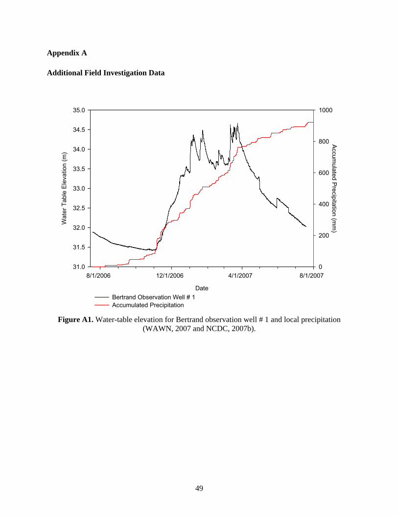
Appendix A
Additional Field Investigation Data
Date
8/1/2006 12/1/2006 4/1/2007 8/1/2007
Wat
er T
able
Ele
vatio
n (m
)
31.0
31.5
32.0
32.5
33.0
33.5
34.0
34.5
35.0
Accumulated Precipitation (m
m)
0
200
400
600
800
1000
Bertrand Observation Well # 1 Accumulated Precipitation
Figure A1. Water-table elevation for Bertrand observation well # 1 and local precipitation
(WAWN, 2007 and NCDC, 2007b).
49

Date
8/1/2006 12/1/2006 4/1/2007 8/1/2007
Wat
er T
able
Ele
vatio
n (m
)
36.5
37.0
37.5
38.0
38.5
39.0
39.5Accum
ulated Precipitation (mm
)
0
200
400
600
800
1000
Bertrand Observation Well # 2Accumulated Precipitation
Figure A2. Water-table elevation for Bertrand observation well # 2 and local precipitation
(WAWN, 2007 and NCDC, 2007b).
50

Date
8/1/2006 12/1/2006 4/1/2007 8/1/2007
Wat
er T
able
Ele
vatio
n (m
)
32.0
32.5
33.0
33.5
34.0
34.5
35.0Accum
ulated Precipitation (mm
)
0
200
400
600
800
1000
Bertrand Observation Well # 3Accumulated Precipitation
Figure A3. Water-table elevation for Bertrand observation well # 3 and local precipitation
(WAWN, 2007 and NCDC, 2007b).
51
Date
8/1/2006 12/1/2006 4/1/2007 8/1/2007
Wat
er T
able
Ele
vatio
n (m
)
29.5
30.0
30.5
31.0
31.5
32.0Accum
ulated Precipitation (mm
)
0
200
400
600
800
1000
Fishtrap Observation Well # 1Accumulated Precipitation
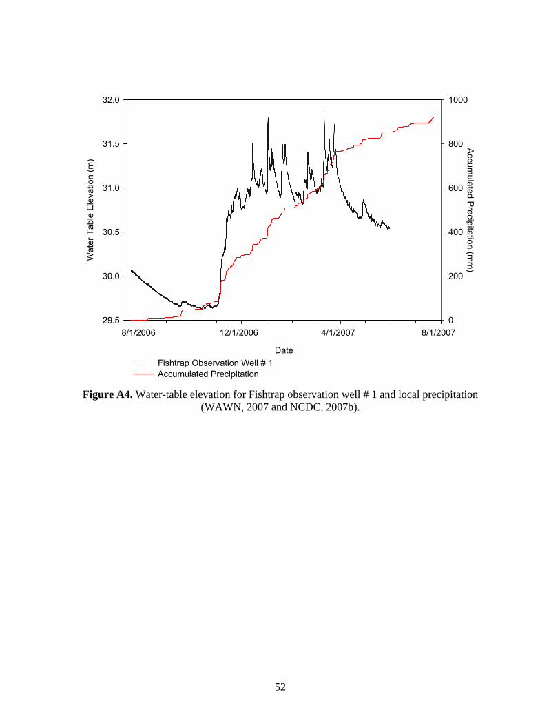
Figure A4. Water-table elevation for Fishtrap observation well # 1 and local precipitation
(WAWN, 2007 and NCDC, 2007b).
52

Date
8/1/2006 12/1/2006 4/1/2007 8/1/2007
Wat
er T
able
Ele
vatio
n (m
)
36.2
36.4
36.6
36.8
37.0
37.2
37.4
37.6
Accumulated Precipitation (m
m)
0
200
400
600
800
1000
Fishtrap Observation Well # 2Accumulated Precipitation
Figure A5. Water-table elevation for Fishtrap observation well # 2 and local precipitation
(WAWN, 2007 and NCDC, 2007b).
53

Date
8/1/2006 12/1/2006 4/1/2007 8/1/2007
Wat
er T
able
Ele
vatio
n (m
)
38.5
39.0
39.5
40.0
40.5
41.0
41.5
42.0Accum
ulated Precipitation (mm
)
0
200
400
600
800
1000
Fishtrap Observation Well # 3Accumulated Precipitation
Figure A6. Water-table elevation for Fishtrap observation well # 3 and local precipitation
(WAWN, 2007 and NCDC, 2007b).
54

Date
8/1/2006 12/1/2006 4/1/2007 8/1/2007
Wat
er T
able
Ele
vatio
n (m
)
31.0
31.5
32.0
32.5
33.0
33.5
34.0
34.5
35.0W
ater Depth (m
)
0
1
2
3
Bertrand Observation Well # 1 Bertrand Creek Water Depth
Figure A7. Water-table elevation for Bertrand observation well # 1 and Bertrand Creek water
depth.
55

Date
7/1/2006 9/1/2006 11/1/2006 1/1/2007 3/1/2007 5/1/2007
Wat
er D
epth
(m)
0.0
0.5
1.0
1.5
2.0
2.5
3.0
3.5A
ccumulated P
recipitation (mm
)
0
200
400
600
800
1000
Bertrand Creek Water DepthAccumulated Precipitation
Figure A8. Bertrand Creek water depth and local precipitation (WAWN, 2007 and NCDC,
2007b).
56

Date
8/1/2006 9/1/2006 10/1/2006 11/1/2006
Wat
er D
epth
(m)
0.2
0.4
0.6
0.8
1.0
1.2
1.4
1.6
Accum
ulated Precipitation (m
m)
0
50
100
150
200
250
300
Fishtrap Creek Water DepthAccumulated Precipitation
Figure A9. Fishtrap Creek water depth and local precipitation (WAWN, 2007 and NCDC,
2007b).
57

Appendix B
Additional Model Boundary Condition Data
Table B1. USGS observation well data (Kimbrough et al., 2004 and 2005).
USGS Well Number
Latitude (DMS)
Longitude (DMS)
Date (mm-dd-yyyy)
Water Table Elevation
(ft) 485607122321401 48°56'02.24" 122°32'18.33" 5/1/1987 39.00 8/15/1990 39.44 10/17/1990 39.88 11/14/1990 42.79 12/18/1990 43.38 1/18/1991 43.76 2/20/1991 42.79 3/14/1991 42.16 3/24/1991 41.50 5/21/1991 41.05 6/26/1991 39.90 7/18/1991 40.05 8/13/1991 39.80 9/25/1991 39.47 10/23/1991 39.52 9/3/2004 39.72 8/29/2005 39.53485700122313401 48°56'59.00" 122°31'39.34" 5/3/1989 73.30 8/14/1990 70.85 9/18/2002 70.07 9/3/2004 69.92 8/29/2005 70.32 3/7/2006 74.13485725122242701 48°57'23.95" 122°24'32.09" 10/22/1997 87.07 10/22/1997 87.02 11/4/1997 86.16 11/11/1997 86.16 4/14/1998 87.74 6/17/1998 87.74 6/17/1998 87.74 8/21/2006 85.83485746122250301 48°57'46" 122°25'03" 8/4/1989 101.00 7/23/1990 105.40 8/27/1990 104.07 10/17/1990 103.76 11/14/1990 105.29 12/17/1990 110.55 1/19/1991 111.50 2/21/1991 111.22 3/14/1991 110.96
58
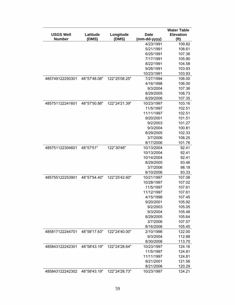
USGS Well Number
Latitude (DMS)
Longitude (DMS)
Date (mm-dd-yyyy)
Water Table Elevation
(ft) 4/23/1991 109.82 5/21/1991 108.61 6/25/1991 107.36 7/17/1991 105.90 8/22/1991 104.58 9/26/1991 103.93 10/23/1991 103.93485749122250301 48°57'48.08" 122°25'08.25" 7/27/1994 106.00 4/16/1998 106.00 9/3/2004 107.36 8/29/2005 108.73 8/29/2006 107.35485751122241601 48°57'50.88" 122°24'21.39" 10/23/1997 103.16 11/5/1997 102.51 11/11/1997 102.51 9/20/2001 101.51 9/2/2003 101.27 9/3/2004 100.81 8/29/2005 102.33 3/7/2006 108.25 8/17/2006 101.76485751122304601 48°57'51" 122°30'46" 10/13/2004 92.41 10/13/2004 92.41 10/14/2004 92.41 8/29/2005 93.46 3/7/2006 98.18 8/10/2006 93.33485755122253901 48°57'54.40" 122°25'42.60" 10/21/1997 107.08 10/28/1997 107.02 11/5/1997 107.61 11/12/1997 107.61 4/15/1998 107.45 9/20/2001 105.92 9/2/2003 105.05 9/3/2004 105.46 8/29/2005 105.64 3/7/2006 107.57 8/16/2006 105.45485817122244701 48°58'17.63" 122°24'40.00" 2/10/1998 122.00 9/3/2004 112.88 8/30/2006 113.70485843122242301 48°58'43.19" 122°24'28.64" 10/23/1997 124.16 11/5/1997 124.81 11/11/1997 124.81 9/21/2001 121.56 8/21/2006 120.29485843122242302 48°58'43.19" 122°24'28.73" 10/23/1997 124.21
59
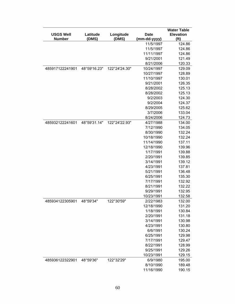
USGS Well Number
Latitude (DMS)
Longitude (DMS)
Date (mm-dd-yyyy)
Water Table Elevation
(ft) 11/5/1997 124.86 11/5/1997 124.86 11/11/1997 124.86 9/21/2001 121.49 8/21/2006 120.33485917122241901 48°59'16.23" 122°24'24.30" 10/24/1997 129.09 10/27/1997 128.89 11/10/1997 130.01 9/21/2001 126.35 8/28/2002 125.13 8/28/2002 125.13 9/2/2003 124.30 9/2/2004 124.37 8/29/2005 125.62 3/7/2006 133.04 8/24/2006 124.73485932122241601 48°59'31.14" 122°24'22.93" 4/27/1988 134.00 7/12/1990 134.05 8/30/1990 132.24 10/18/1990 132.24 11/14/1990 137.11 12/18/1990 139.96 1/17/1991 139.88 2/20/1991 139.85 3/14/1991 139.12 4/23/1991 137.81 5/21/1991 136.48 6/25/1991 135.30 7/17/1991 132.92 8/21/1991 132.22 9/29/1991 132.95 10/23/1991 132.58485934122305901 48°59'34" 122°30'59" 2/22/1983 132.00 12/18/1990 131.20 1/18/1991 130.84 2/20/1991 131.18 3/14/1991 130.98 4/23/1991 130.80 6/6/1991 130.24 6/25/1991 129.98 7/17/1991 129.47 8/22/1991 128.99 9/25/1991 129.26 10/23/1991 129.15485936122322901 48°59'36" 122°32'29" 6/9/1980 195.00 8/10/1990 189.48 11/16/1990 190.15
60

USGS Well Number
Latitude (DMS)
Longitude (DMS)
Date (mm-dd-yyyy)
Water Table Elevation
(ft) 2/20/1991 191.07 3/14/1991 191.18 5/21/1991 190.82 6/25/1991 189.59 7/17/1991 190.10 8/22/1991 189.50 9/25/1991 189.90 10/23/1991 190.01
61

Appendix C
Numerical Ground-Water Model Hydraulic Conductivity Zones
Shown below are the hydraulic conductivity zones defined by Scibek and Allen (2005) within
the study area for model layers 2-5.
Figure C1. Hydraulic conductivity zones for model layer 2. Units are in m/d.
62
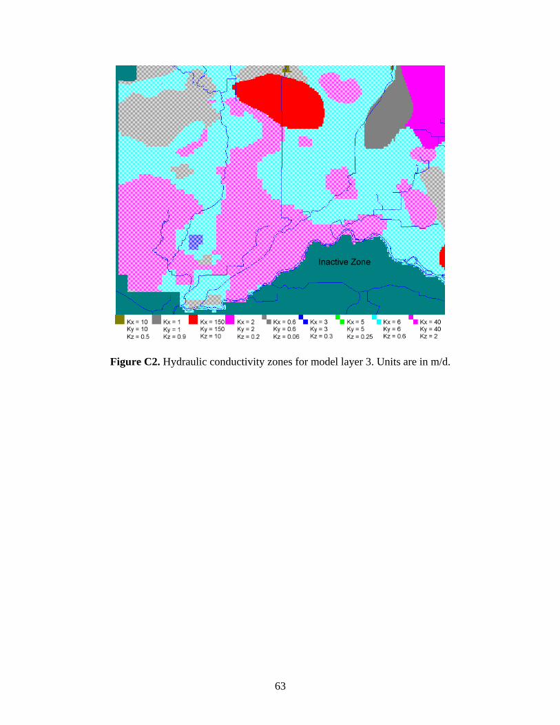
Figure C2. Hydraulic conductivity zones for model layer 3. Units are in m/d.
63

Figure C3. Hydraulic conductivity zones for model layer 4. Units are in m/d.
64
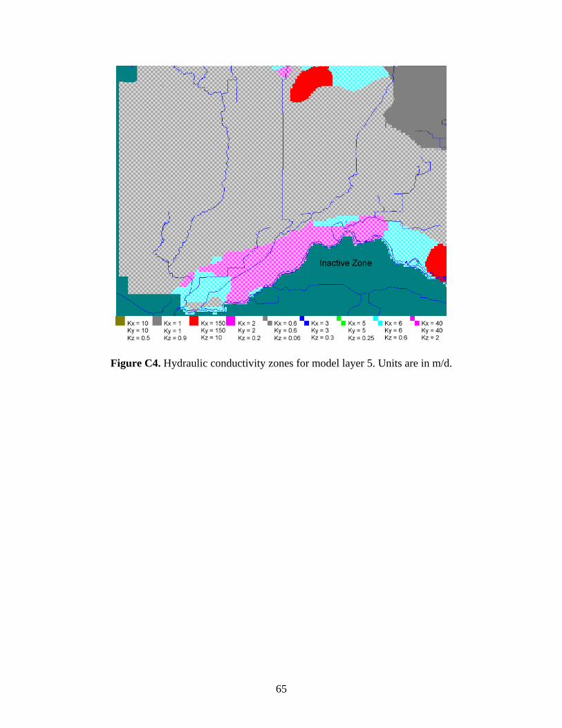
Figure C4. Hydraulic conductivity zones for model layer 5. Units are in m/d.
65

Appendix D
STELLA Model Screen Captures
Figure D1. Screen capture of STELLA model title screen.
66

Figure D2. Screen capture of STELLA model. User can view background information, and restore switches and sliders to default values.
Figure D3. Screen capture of STELLA model. User is asked to choose a region of interest.
67
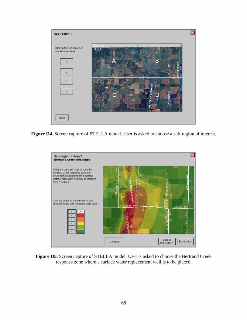
Figure D4. Screen capture of STELLA model. User is asked to choose a sub-region of interest.
Figure D5. Screen capture of STELLA model. User is asked to choose the Bertrand Creek response zone where a surface water replacement well is to be placed.
68

Figure D6. Screen capture of STELLA model. User is asked to choose the Fishtrap Creek response zone where a surface water replacement well is to be placed.
Figure D7. Screen capture of STELLA model. User is asked to select the creek for which surfacewater is to be exchanged for groundwater.
69
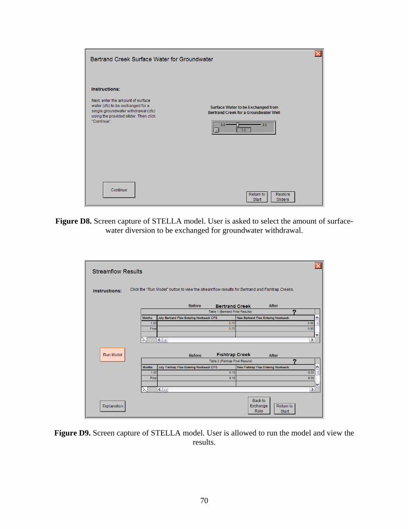
Figure D8. Screen capture of STELLA model. User is asked to select the amount of surface-water diversion to be exchanged for groundwater withdrawal.
Figure D9. Screen capture of STELLA model. User is allowed to run the model and view the results.
70