Use of moment generating functions

1. Using the moment generating functions of X, Y, Z, …determine the moment generating function of W = h(X, Y, Z, …).

2. Identify the distribution of W from its moment generating function

This procedure works well for sums, linear combinations etc.

TheroremLet X and Y denote a independent random variables each having a gamma distribution with parameters (,1) and (,2). Then W = X + Y has a gamma distribution with parameters (, 1 + 2).

Proof:

1 2

and X Ym t m tt t

1 2 1 2

t t t

Therefore X Y X Ym t m t m t

Recognizing that this is the moment generating function of the gamma distribution with parameters (, 1 + 2) we conclude that W = X + Y has a gamma distribution with parameters (, 1 + 2).

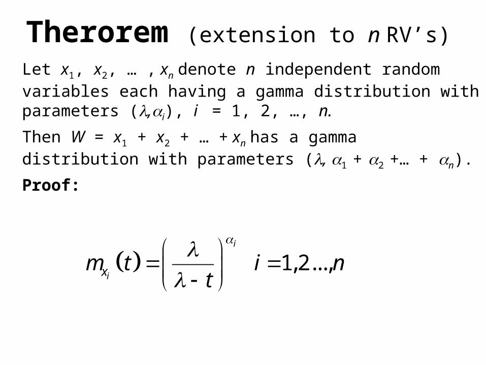
Therorem (extension to n RV’s)

Let x1, x2, … , xn denote n independent random variables each having a gamma distribution with parameters (,i), i = 1, 2, …, n.

Then W = x1 + x2 + … + xn has a gamma distribution with parameters (, 1 + 2 +… + n).

Proof:

1, 2...,i

ixm t i nt

1 2 1 2 ...

...n n

t t t t

1 2 1 2... ...

n nx x x x x xm t m t m t m t

Recognizing that this is the moment generating function of the gamma distribution with parameters (, 1 + 2 +…+ n) we conclude that

W = x1 + x2 + … + xn has a gamma distribution with parameters (, 1 + 2 +…+ n).

Therefore

TheroremSuppose that x is a random variable having a gamma distribution with parameters (,).

Then W = ax has a gamma distribution with parameters (/a, ).

Proof: xm t

t

then ax xam t m at

at ta

1. Let X and Y be independent random variables having a 2 distribution with 1 and 2 degrees of freedom respectively then X + Y has a 2

distribution with degrees of freedom 1 + 2.

Special Cases

2. Let x1, x2,…, xn, be independent random variables having a 2 distribution with 1 , 2 ,…, n degrees of freedom respectively then x1+ x2 +…+ xn has a 2 distribution with degrees of freedom 1 +…+ n.

Both of these properties follow from the fact that a 2 random variable with degrees of freedom is a random variable with = ½ and = /2.

If z has a Standard Normal distribution then z2 has a 2 distribution with 1 degree of freedom.

Recall

Thus if z1, z2,…, z are independent random variables each having Standard Normal distribution then

has a 2 distribution with degrees of freedom.

2 2 21 2 ...U z z z

TheroremSuppose that U1 and U2 are independent random variables and that U = U1 + U2 Suppose that U1 and U have a 2 distribution with degrees of freedom 1and respectively. (1 < )

Then U2 has a 2 distribution with degrees of freedom 2 = -1

Proof:

12

1

12

12

Now

v

Um tt

21

2

12

and

v

Um tt

1 2

Also U U Um t m t m t

2

12 2

12

12

1122

11 22

12

v

vv

v

t

t

t

2

1

Hence UU

U

m tm t

m t

Q.E.D.

Distribution of the sample variance

2

2 1

( )

1

n

ii

x xs

n

Properties of the sample variance

Proof:

2 2

1 1

( ) ( )n n

i ii i

x x x a a x

2 2

1

( ) 2( )( ) ( )n

i ii

x a x a x a x a

2 2 2

1 1

( ) ( ) ( )n n

i ii i

x x x a n x a

2 2

1 1

( ) 2( ) ( ) ( )n n

i ii i

x a x a x a n x a

2 2 2

1

( ) 2 ( ) ( )n

ii

x a n x a n x a

2 2

1

( ) ( )n

ii

x a n x a

Special Cases

2 2 2

1 1

( ) ( ) ( )n n

i ii i

x x x a n x a

2

12 2 2 2

1 1 1

( )

n

in n ni

i i ii i i

x

x x x nx xn

1. Setting a = 0.

Computing formula

2 2 2

1 1

( ) ( ) ( )n n

i ii i

x x x n x

2. Setting a = .

2 2 2

1 1

or ( ) ( ) ( )n n

i ii i

x x x n x

Distribution of the sample variance

Let x1, x2, …, xn denote a sample from the normal distribution with mean and variance 2.

11 , , n

n

xxz z

Let

22 2 11 2

n

ii

n

xz z

Then

has a 2 distribution with n degrees of freedom.

Note:

2 22

1 12 2 2

( ) ( )( )

n n

i ii i

x x xn x

or U = U2 + U1

2

12

( )n

ii

xU

has a 2 distribution with n degrees of freedom.

has normal distribution with mean and variance 2/n

xz

n

Thus

221 2

n xU z

has a 2 distribution with 1 degree of freedom.

We also know that x

has a Standard Normal distribution and

If we can show that U1 and U2 are independentthen

22

12 2 2

( )( 1)

n

ii

x xn s

U

has a 2 distribution with n - 1 degrees of freedom.

The final task would be to show that

are independent

2

1

( ) and n

ii

x x x

2

21

2 2

( )1

n

ii

x xn s

U

Summary

Let x1, x2, …, xn denote a sample from the normal distribution with mean and variance 2.

2.

has a 2 distribution with = n - 1 degrees of freedom.

1. than has normal distribution with mean and variance 2/n

x

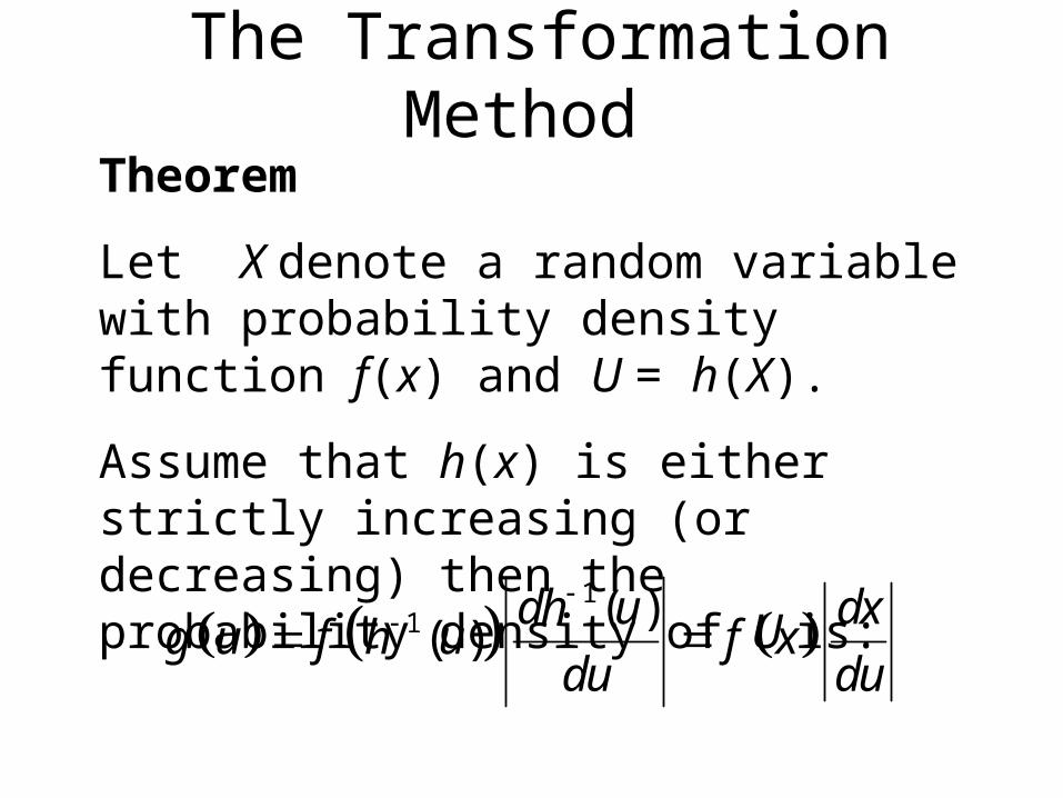
The Transformation Method

Theorem

Let X denote a random variable with probability density function f(x) and U = h(X).

Assume that h(x) is either strictly increasing (or decreasing) then the probability density of U is:

1

1 ( )( )

dh u dxg u f h u f x

du du

Proof

Use the distribution function method.

Step 1 Find the distribution function, G(u)

Step 2 Differentiate G (u ) to find the probability density function g(u)

G u P U u P h X u

1

1

( ) strictly increasing

( ) strictly decreasing

P X h u h

P X h u h

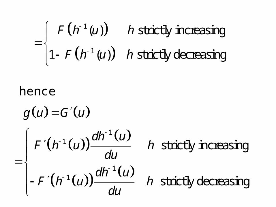
1

1

( ) strictly increasing

1 ( ) strictly decreasing

F h u h

F h u h

hence

g u G u

11

11

strictly increasing

strictly decreasing

dh uF h u h

du

dh uF h u h

du

or

1

1 ( )( )

dh u dxg u f h u f x

du du

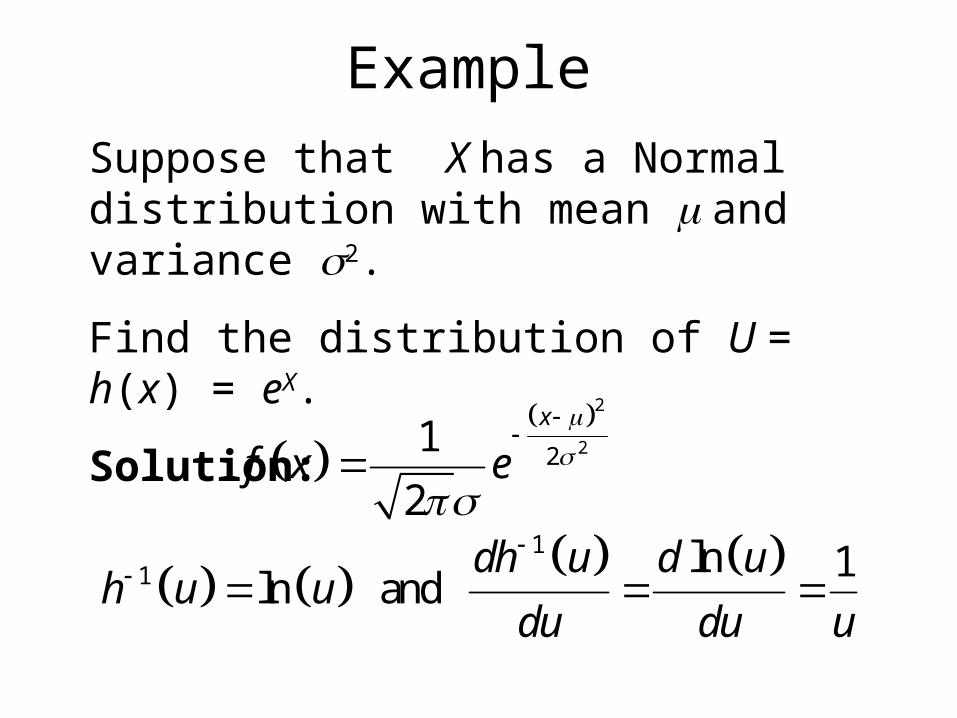
Example

Suppose that X has a Normal distribution with mean and variance 2.

Find the distribution of U = h(x) = eX.

Solution:

2

221

2

x

f x e

11 ln 1

ln and dh u d u

h u udu du u

hence

1

1 ( )( )

dh u dxg u f h u f x

du du

22

ln

21 1 for 0

2

u

e uu

This distribution is called the log-normal distribution

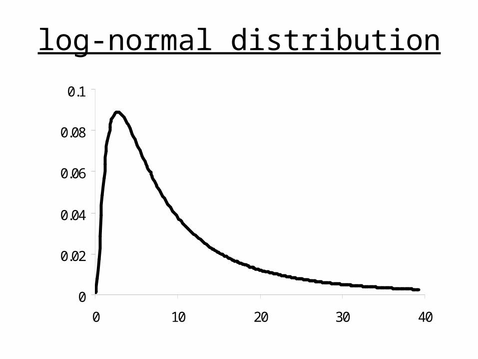
log-normal distribution

0

0.02

0.04

0.06

0.08

0.1

0 10 20 30 40

The Transfomation Method(many variables)

Theorem

Let x1, x2,…, xn denote random variables with joint probability density function

f(x1, x2,…, xn )

Let u1 = h1(x1, x2,…, xn).u2 = h2(x1, x2,…, xn).

un = hn(x1, x2,…, xn).

define an invertible transformation from the x’s to the u’s

Then the joint probability density function of u1, u2,…, un is given by:

11 1

1

, ,, , , ,

, ,n

n nn

d x xg u u f x x

d u u

1, , nf x x J

where

1

1

, ,

, ,n

n

d x xJ

d u u

Jacobian of the transformation

1 1

1

1

detn

n n

n

dx dx

du du

dx dx

du du

ExampleSuppose that x1, x2 are independent with density functions f1 (x1) and f2(x2)

Find the distribution of

u1 = x1+ x2

u2 = x1 - x2

Solving for x1 and x2 we get the inverse transformation

1 21 2

u ux

1 22 2

u ux

1 2

1 2

,

,

d x xJ

d u u

The Jacobian of the transformation

1 1

1 2

2 2

1 2

det

dx dx

du du

dx dx

du du

1 11 1 1 1 12 2det

1 1 2 2 2 2 2

2 2

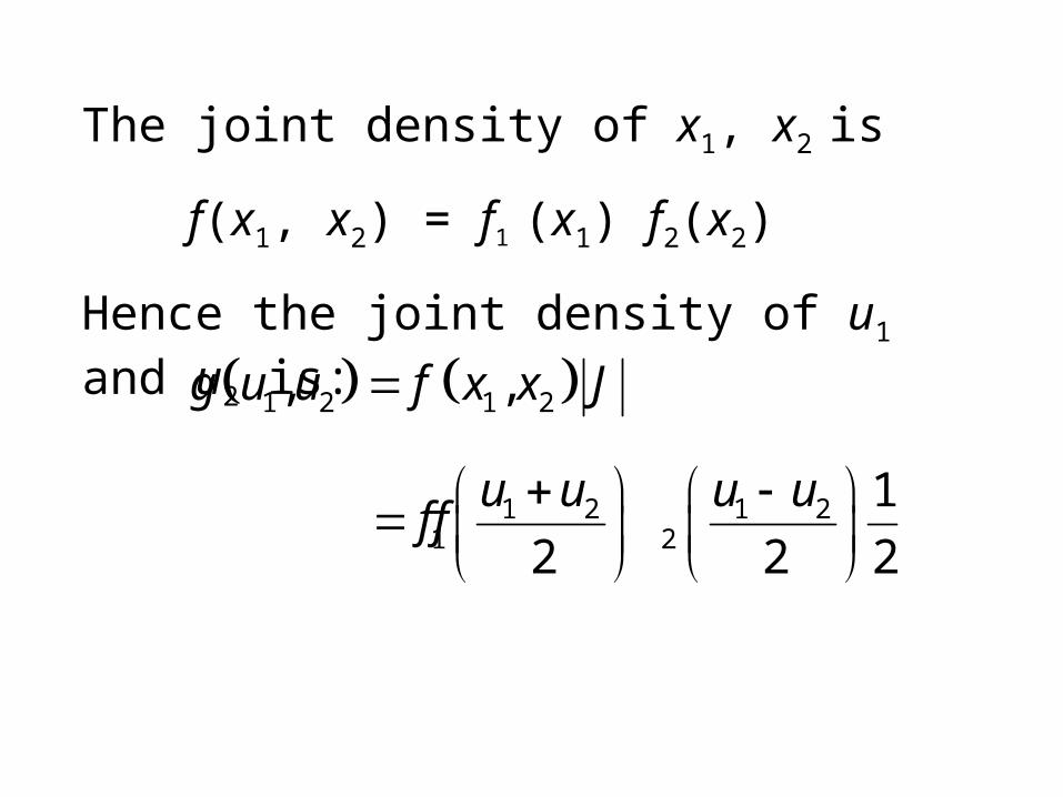
The joint density of x1, x2 is

f(x1, x2) = f1 (x1) f2(x2)

Hence the joint density of u1 and u2 is:

1 2 1 21 2

1

2 2 2

u u u uf f

1 2 1 2, ,g u u f x x J

From

1 2 1 21 2 1 2

1,

2 2 2

u u u ug u u f f

We can determine the distribution of u1= x1 + x2

1 1 1 2 2,g u g u u du

1 2 1 2

1 2 2

1

2 2 2

u u u uf f du

1 2 1 21

2

1put then ,

2 2 2

u u u u dvv u v

du

Hence

1 2 1 21 1 1 2 2

1

2 2 2

u u u ug u f f du

1 2 1f v f u v dv

This is called the convolution of the two densities f1 and f2.

Example: The ex-Gaussian distribution

1. X has an exponential distribution with parameter .

2. Y has a normal (Gaussian) distribution with mean and standard deviation .

Let X and Y be two independent random variables such that:

Find the distribution of U = X + Y.

This distribution is used in psychology as a model for response time to perform a task.

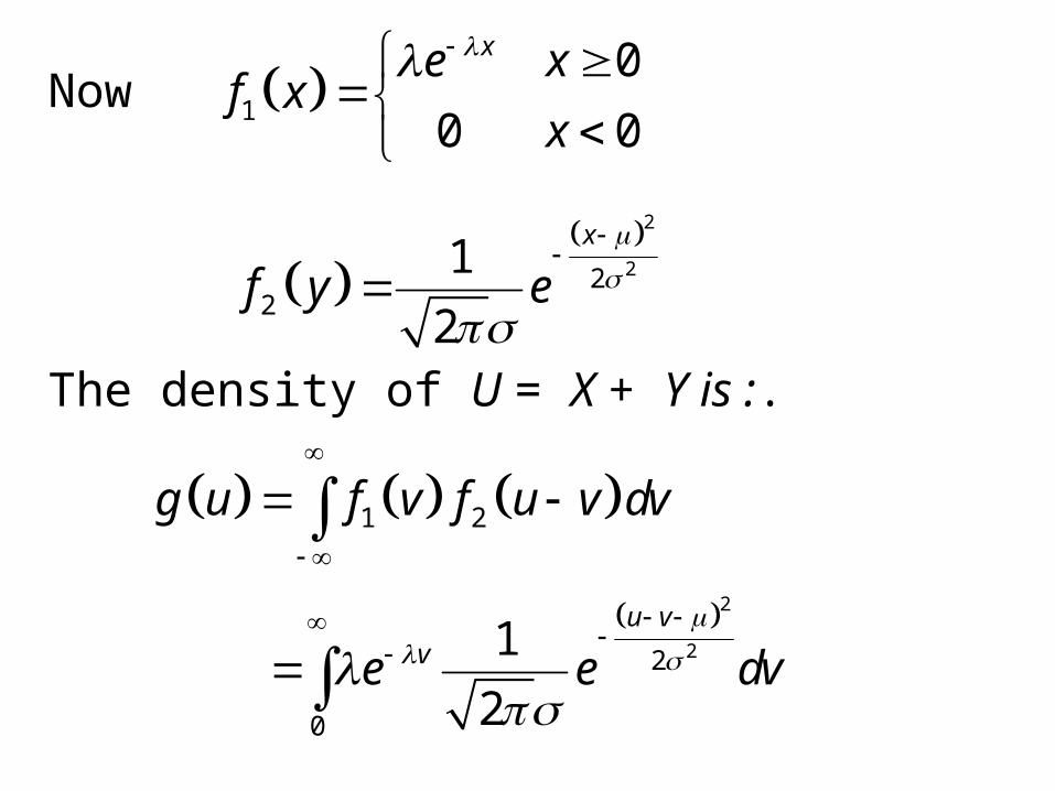
Now 1

0

0 0

xe xf x

x

1 2g u f v f u v dv

The density of U = X + Y is :.

2

222

1

2

x

f y e

222

0

1

2

u vve e dv

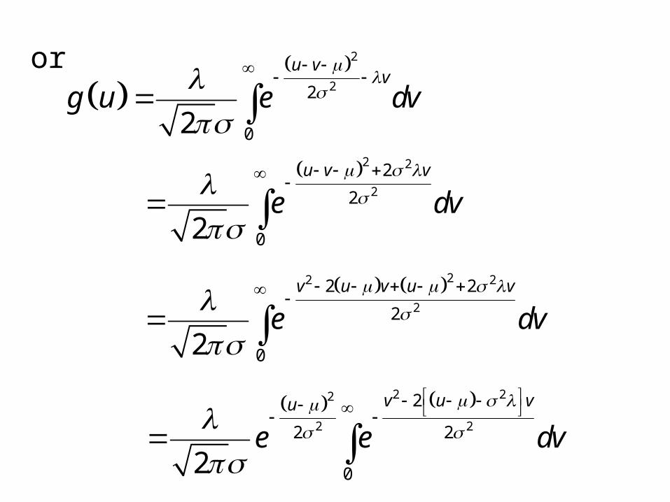
or

2

22

02

u vv

g u e dv

2 2

2

2

2

02

u v v

e dv

22 2

2

2 2

2

02

v u v u v

e dv

2 22

2 2

2

2 2

02

v u vu

e e dv

or 2 22

2 2

2

2 2

02

v u vu

e e dv

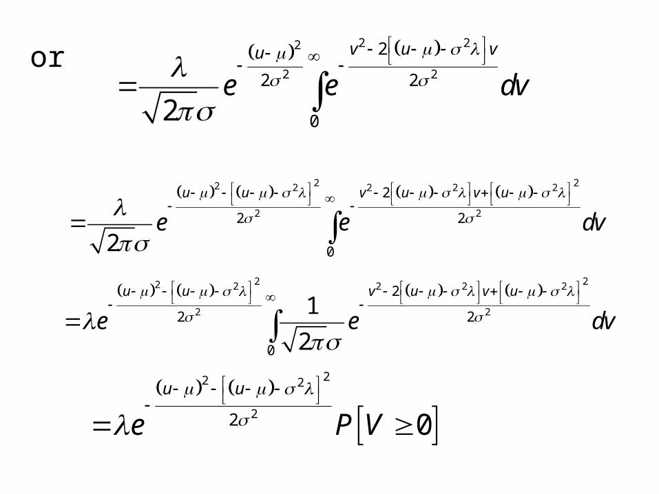
2 22 2 2 2 2

2 2

2

2 2

02

u u v u v u

e e dv

2 22 2 2 2 2

2 2

2

2 2

0

1

2

u u v u v u

e e dv

22 2

22 0u u

e P V

Where V has a Normal distribution with mean

22

2

21

u ug u e

2V u

and variance 2.

Hence

Where (z) is the cdf of the standard Normal distribution

0

0.03

0.06

0.09

0 10 20 30

g(u)

The ex-Gaussian distribution