Use of GPR and MASW to Complement Backcalculated Moduli and Design Life Calculations

Edmund Surette, Ph.D. Candidate Dalhousie University

Christopher Barnes, Ph.D., P.Eng.

Dalhousie University

Nouman Ali, Ph.D., P.Eng. Dalhousie University

Paper prepared for presentation at the “Pavement Evaluation, Performance and Management” Poster Session

2010 Annual Conference of the Transportation Association of Canada

Halifax, Nova Scotia

  2

ABSTRACT Nondestructive deflection testing by means of the falling weight deflectometer is one of the most reliable and established methods for evaluating the structural capacity of pavements. However, there are several factors that can influence the moduli values obtained through the backcalculation process and the resulting calculated design life or required overlay thickness. Some of the difficulties associated with backcalculation include constructing a suitable pavement model due to the as-built variations in layer thicknesses in addition to determining the modulus for thin asphalt layers. Many researchers have reported success when using ground penetrating radar (GPR) to determine flexible pavement layer thicknesses. Recently, the Multi-Channel Analysis of Surface Waves (MASW) technique has been shown to provide accurate non-destructive estimates of the in-situ asphalt concrete modulus. In this study, nondestructive deflection testing in addition to GPR and MASW testing was performed along a 200 m test section and across the transverse width of the traffic lane to establish variations in thickness and moduli. Backcalculation was performed with and without GPR thickness data resulting in a 40% variation in modulus. The modulus obtained via GPR data provided a significantly better estimate to the recorded MASW modulus. Using the 1993 AASHTO Guide for Design of Pavement Structures, the difference in modulus and thickness between GPR and non GPR data resulted in nearly a two inch difference in required overlay thickness. The results obtained using the new Mechanistic-Empirical Pavement Design Guide (MEPDG) identified considerable differences in rutting performance, but only minute differences in asphalt fatigue. INTRODUCTION With the release of the new Mechanistic-Empirical Pavement Design Guide (MEPDG), pavement design technology is currently undergoing a major upgrade. The MEPDG which is intended to supersede the 1993 AASHTO Guide for Design of Pavement Structures uses key material characterization inputs such as the dynamic modulus for asphalt concrete layers and the resilient modulus for granular layers to design suitable overlays that will extend the service life of the pavement system. Nondestructive testing such as deflection testing by means of the falling weight deflectometer (FWD), ground penetrating radar (GPR), and seismic methods, is also highly recommended for the evaluation of existing pavements for rehabilitation. A large number of highway agencies are now in the process of implementing or are developing studies to prepare adoption of the new MEPDG. The traditional method used to determine the dynamic modulus of asphalt concrete involves subjecting cylindrical samples to sinusoidal loading at various frequencies and temperatures. This method requires sophisticated and expensive testing equipment which may not be available to all transportation agencies and involves extracting core samples from in-situ pavements. Accordingly, FWD testing has become the primary means of characterizing the in-situ properties of flexible pavements (Park et al. 2001). Using a process known as backcalculation, layer moduli can be determined for a particular pavement using the recorded deflection values. However, literature has shown (Ullidzt and Stubstad 1985; Irwin 2002) that there are several factors that can influence the results obtained through the backcalculation process. Two of these factors include variations in pavement layer thicknesses and the insensitivity in computing the

  3

modulus of thin asphalt layers. Consequently, the errors in the backcalculated moduli will modify the requirements for an appropriate pavement design. Conventionally, pavement layer thicknesses have been established using destructive techniques such as coring or drilling bore holes which are time consuming and do not provide continuous thickness data. In recent years, GPR has been shown to be a valuable nondestructive tool in assessing pavement layer thickness (Maser et al. 2006). As a result, some agencies now specify the use of GPR when performing deflection testing. Seismic surface wave propagation methods which include the steady state Rayleigh wave method (Jones 1955) and Spectral Analysis of Surface Waves (SASW) (Heisey et al. 1982, Nazarian et al. 1983) have been utilized in determining layer moduli for pavement and geotechnical engineering purposes for over 50 years. More recently, Multi-channel Simulation with One Receiver (MSOR) (Ryden et al. 2003) and the Multi-Channel Analysis of Surface Waves (MASW) (Park et al. 1999; Barnes et al. 2008) technique have shown to provide accurate non-destructive estimates for computing the in-situ asphalt concrete modulus of the top surface layer. An experimental study was conducted to compare pavement layer thicknesses determined from GPR and conventional destructive techniques and to establish the effect on the backcalculated moduli and resultant design requirements. Moduli values computed from the MASW test were compared to traditional dynamic modulus testing and were used to validate the backcalculated moduli values. FALLING WEIGHT DEFLECTOMETER One of the most reliable methods used to evaluate the structural capacity and remaining serviceable life of in-situ pavements is to use nondestructive deflection testing. The impulse devices, particularly the falling weight deflectometer (FWD), are recently developed and are currently the most used by highway and airport agencies (Shahin 1994). The FWD consists of a drop-mass system where a weight can be lifted to various heights and then dropped to produce the desired impulse force. A load cell and several velocity transducers or geophones measure the magnitude of the load in addition to the deflections at different offset positions from the load center. One important characteristic of the FWD is that the load applied to the pavement structure is comparable to highway traffic loading with regards to both frequency and magnitude. From the measured deflections and load magnitude, in addition to other input parameters such as pavement layer thickness, the analyzer is capable of computing the various layer moduli using a process known as backcalculation. Backcalculation is an iterative process that takes the measured surface deflection and attempts to match it with a theoretical surface deflection generated from an identical pavement structure using assumed layer moduli. The assumed layer moduli in the theoretical model are adjusted until they produce a surface deflection that closely matches the measured one, within a specified tolerance. The backcalculation process is normally completed using computer software.

  4

Several factors can influence the assumed moduli values which can lead to erroneous results (Irwin 2002). First, it is extremely important to create a closely matching theoretical pavement model to the in-situ conditions. In many situations this can be a difficult task as layer thicknesses are often not known or may vary substantially throughout a pavement section and subsurface layers may be overlooked. In addition, some pavement layers are too thin to be backcalculated in the pavement model. This phenomenon is termed sensitivity and can occur if a layer is too thin for its modulus to have an influence on the surface deflections. If the deflection is insensitive to the layer modulus, then any backcalculated value for that layer may suffice. To overcome some of these concerns, additional destructive or nondestructive testing may be implemented in conjunction with the FWD. GROUND PENETRATING RADAR Many researchers (Al-Qadi et al. 2004; Willett et al. 2006) have reported success when using ground penetrating radar (GPR) technology to measure flexible pavement layer thickness. In pavement design, GPR is generally used to determine pavement layer thickness as a complement or replacement to coring and test pits. In many instances, GPR is considered to be a better alternative to coring as it is a quick nondestructive method which provides continuous thickness data collected near or at highway speeds (Maser et al. 2006). The primary components of a GPR system include a control unit with associated software for data collection and processing and one or several radar antennas for emitting and receiving electromagnetic waves. Depending on the type of antenna that is used for pavement evaluation, GPR systems are classified as either air coupled or ground coupled. In the air-coupled systems, the “horn” antennas are typically suspended 150 – 500 mm above the surface for operation at highway speeds (up to 80km/h). These systems provide a clean radar signal, although the depth of penetration is limited because part of the electromagnetic energy sent by the antenna is reflected back by the pavement surface. Conversely, the antennas used in the ground coupled systems are in full contact with the ground surface providing a higher depth of penetration at the same frequency, but limiting the survey speed. The short electromagnetic waves travel through the pavement’s layers and reflect off surfaces or objects that exhibit discontinuities in electrical properties, for example different materials, changes in moisture content, or changes in density (Loizos et al. 2007). The intensity of the reflected pulses is directly proportional to the contrast in dielectric constant between adjacent materials. The reflected pulses are received by the antenna and are recorded as waveforms which are digitized and interpreted by computing the amplitude and arrival times from each main reflection (Maser et al. 2006). In order to calculate the thickness, the dielectric constant of the material must be known. The dielectric value can either be calibrated based on measured thicknesses (cores, test pits etc.) or can be estimated nondestructively. Using the horn antenna, the dielectric constant of HMA is estimated by using the amplitude of the reflected signal from a metallic plate placed on the pavement surface and the amplitude of the reflected signal from the surface. For the horn antenna method, the pavement thickness can be computed from the amplitudes and arrival times using Eq. (1). (Al Qadi et al. 2004; Loizos et al. 2007)

  5

i

ii

cth

ε2= (1)

Where, hi = the thickness of the ith layer, ti = the electromagnetic wave two way travel time through the ith layer, c = the speed of light in free space, and εi = the dielectric constant of the ith layer. For the ground coupled systems which are in direct contact with the pavement surface, the equations displayed for the horn antenna method cannot be used because the radar wave does not travel through air. Consequently, the dielectric constant cannot be calculated directly from the data and needs to be calibrated from core samples. Based on the Pythagorean Theorem, Eq. (2) can be constructed for layer thickness.

22)(5.0 dVth −= (2) Where h = the layer thickness, V = the electromagnetic wave velocity, t = the total recorded travel time, and d = distance between the transmitter and the receiver units within the antenna. SEISMIC SURFACE WAVE PROPAGATION METHODS Surface waves are stress waves that propagate along the free surface of a material. The velocity of wave propagation is dependent on the elastic properties of the material and consequently can be used to estimate the elastic modulus. Several techniques including Spectral Analysis of Surface Waves (SASW), Multi-Channel Simulation with One Receiver (MSOR) and Multi-channel Analysis of Surface Waves (MASW) have been used in determining the asphalt concrete modulus in a pavement system (Nazarian et al. 1983, Ryden et al. 2004, Barnes et al. 2009-2). When the surface of an elastic medium is impacted, two types of stress waves will be generated, body waves and surface waves. Body waves consist of compression waves (P wave) and shear waves (S wave) which propagate radially outward from the load point along a hemispherical wave front within the elastic medium. The surface wave, also called Rayleigh wave, does not propagate into the body of the elastic medium, but rather travels along the surface of the half space. Surface wave testing uses the dispersive nature of Rayleigh waves in a layered medium to evaluate the elastic stiffness properties of the different layers (Ryden et al. 2004). Dispersion is defined as the variation of Rayleigh wave velocity with frequency (wavelength) where the stiffness changes with depth. In recent years, a new approach to surface wave testing has been introduced to avoid some of the problems encountered with SASW (Ryden et al. 2004). This new approach, which was used in this research, is based on the MASW data processing technique and the MSOR method of data acquisition. In the MSOR method a multichannel record is obtained with only one receiver which is fixed at a surface point and receives signals from impacts at incremental offsets (Ryden

  6

et al. 2001). It has been shown (Ryden et al. 2003) that the fundamental symmetric and anti-symmetric free plate Lamb wave modes dominate for wavelengths within plates that are supported by significantly less stiff material. MASW has proven (Park et al. 1998, 1999) to be an effective technique of developing Rayleigh dispersion curves by identifying and tracking the approximate fundamental Lamb wave modes which asymptotically approach the fundamental Rayleigh wave mode. Once the phase velocities have been determined the shear wave velocity may be estimated and the modulus is calculated by means of Eq. (3) (Ryden et al. 2006).

)1)((2 2 νρ += sVE (3) The modulus that is determined using surface wave methods is considered to be a high frequency modulus, with velocity data obtained at frequencies ranging between 10 and up to 90 kHz. In general, the traffic and FWD frequency used in design is in the range of 10-25 Hz. As a result, the asphalt concrete master curve defined in the next section may be used to shift the high frequency moduli to a design value (Barnes et al. 2009-1). DYNAMIC MODULUS MASTER CURVE Dynamic modulus testing is typically conducted on a servo-controlled hydraulic machine using cylindrical specimens subjected to a compressive haversine or sine wave load at a given temperature and loading frequency. Strain gauges or LVDTs are positioned on opposite sides of the specimen to measure the vertical deflections. During the test, the axial strain on the specimen is maintained between 50 and 150 microstrain to ensure linear elastic behavior. For linear viscoelastic materials such as hot mix asphalt (HMA) mixtures, the stress-strain relationship under a continuous sinusoidal load is defined by its complex dynamic modulus (E*) (Witczack et al. 2004). The complex modulus is defined as the ratio of the amplitude of the sinusoidal stress (σ) at any given time (t) and the angular load frequency (ω) to the corresponding sinusoidal strain (ε) at the same time. Due to the viscoelasticity, a phase lag (ø) separates the stress from the strain. The sinusoidal stress and strain are defined by Eq. (4) and Eq. (5) respectively.

(4)

(5)

Where, σ0 = stress amplitude and ε0 = strain amplitude. The complex dynamic modulus consists of two components, the storage modulus (E´) (real part) that describes the elastic component and the loss modulus (E´´) (imaginary part) which describes the viscous component. These are determined based on Eq. (6) and (7).

φεσ

cos'0

0=E (6)

)sin(0 tωσσ ⋅=  

)sin(0 φωεε −⋅= t  

  7

φεσ

SinE0

0'' = (7)

The dynamic modulus is defined as the absolute value of the complex modulus, E*, which is the sum of the storage and loss moduli as shown in Eq. (8). The dynamic modulus can be computed by dividing the maximum load by the maximum strain.

0

0'''*εσ

=+= iEEE (8)

Due to the viscoelastic properties of asphalt concrete, the computed dynamic modulus varies with load frequency and temperature. Typically, it increases with increasing loading frequency and with decreasing temperature. The relationship between the modulus, frequency and temperature can be expressed by a master curve which is usually constructed at a reference temperature, generally 20˚C. The master curve enables the prediction of the moduli at any loading frequency or temperature and assists in the comparison of data on an equal basis. The master curve of asphalt concrete can be mathematically modeled by a sigmoidal function described by Eq. (9) proposed by Pellinen et al. 2004.

(9)

Where |E*| = dynamic complex modulus, ξ = reduced frequency, δ = minimum modulus value, α = span of modulus values, and β, γ = shape parameters. The master curve is constructed using the principle of time-temperature superposition. The tested dynamic modulus results at various temperatures and frequencies are shifted to a reduced frequency at an arbitrarily selected reference temperature, T0, as shown in Eq. (10).

( ) ( ) ( )[ ]Taf logloglog +=ξ (10) Where, a(T) = shift factor, a(T0) = 0, f = frequency, and ξ = reduced frequency. The shift factor a(T) can be represented as a second order polynomial function of the temperature, T (Witczak et al. 2004) as shown in Eq. (11).

(11) Where a(T) = shift factor at temperature T, and a, b and c = coefficients of the second order polynomial. The master curve is constructed by simultaneously solving the four coefficients of the sigmoidal function (δ, α, β, γ) and the three coefficients of the second order polynomial (a, b, c). This is completed by optimizing the theoretical model to fit the experimental data by adjusting the coefficients using the “Solver” function in Excel until the least square error is minimized.

)(log*

1)( ξγβ

αδ −++=

eELog  

( )[ ] cbTaTTaLog ++= 2  

  8

EXPERIMENTAL TESTING AND RESULTS Site Description As part of a multiyear research project between Dalhousie University and the Nova Scotia Department of Transportation and Infrastructure Renewal (NSTIR), three 200 meter test sites throughout the province of Nova Scotia were selected for nondestructive testing evaluation (NDT). The nondestructive testing conducted included FWD, GPR, and MASW testing. In addition to the nondestructive tests, the sections were cored for calibration purposes and during construction instrumentation was placed within the pavement structure. For this particular study, the test section selected was located on Highway 103, near Barrington, Nova Scotia. The highway was constructed in 2006 and is a 2-lane controlled access arterial highway. The pavement section, shown in Figure 1, was designed as per the highway design standards utilized by NSTIR. This type of cross section is commonly seen in the majority of Nova Scotia arterial highways. The pavement structure is composed of two asphalt type B-HF lifts approximately 50 mm in thickness, and a 50 mm thick asphalt type C-HF lift. The granular base is considered to be a type I granular material with a maximum size of ¾ inch while the subbase is a type II granular material with maximum size of 1 ½ inches. Figure 1. Typical Pavement Cross Section Coring and Trenching During highway construction, instrumentation was placed at the top of the subgrade and throughout the granular layers located at the midpoint of the 200 meter section. This was completed by trenching a section of the roadway, installing the sensors and then backfilling and compacting with a plate tamper. During this process, the subbase and base thicknesses were measured to be 550 mm and 150 mm respectively, for a total of 700 mm.

 

  9

Once paving was completed, core samples were extracted from the outer wheel path at various stations along the 200 meter section. The cores were then used to determine the asphalt thickness, calibrate the GPR data, and also to perform dynamic modulus testing. The thickness measurements are displayed in Table 1. Table 1. Asphalt Core Thicknesses

Station (m) Thickness (mm)

15 133 55 156 85 174 135 162 175 163

Dynamic Modulus and Master Curve The cores extracted for thickness determination were also used for dynamic modulus test specimens. The cores ranged from 136 mm to 175 mm in thickness and were tested with a servo-hydraulic testing system according to AASHTO TP 62-03 and ASTM D3497. The samples were tested at frequencies of 0.1, 1, 5, 10, and 25 Hz at temperatures of -15, 0, 10, 20, and 40°C using a controlled environmental chamber with an accuracy of ±0.5˚C. The resultant master curve, sigmoidal curve fitting parameters, and shift factor coefficients are displayed in Figure 2. The master curve was used to shift high frequency moduli values from surface wave testing to a 10Hz FWD value in addition to shifting moduli values collected at various temperatures to a standard 20°C value. The dynamic modulus at 20°C and 10Hz frequency was determined to be 3469 MPa. Figure 2. Dynamic Modulus Master Curve

  10

Temperature Measurement The pavement response under an applied load is temperature dependent and therefore pavement temperature must be recorded for each test station. During all NDT, the temperature at mid-depth of the asphalt concrete layer was measured and used as the average temperature for moduli backcalculation and MASW analysis. All calculated moduli values were then shifted from the corresponding measured temperature value to a standard 20°C value using the constructed master curve. Ground Penetrating Radar

Ground penetrating radar (GPR) testing was conducted along the entire 200 meter test section in the outer wheel path to determine the longitudinal variation in pavement thickness. In addition, GPR was used to determine the transverse variation in thickness at both Station 10 and Station 180. The GPR system used in this research was the SIRveyor SIR-20 manufactured by Geophysical Survey Systems, Inc. (GSSI). Two ground coupled antennas were implemented in the analysis. A 1.6GHz antenna was employed to detect the thickness of the asphalt concrete layer, while a 900MHz antenna clearly identified the base layers. The antennas were mounted in a plastic sled and towed behind the test vehicle as shown in Figure 3. Radan 6.5 analysis software manufactured by GSSI was implemented in the analysis and the cores extracted from the site were used to calibrate the GPR data. The results of the longitudinal asphalt concrete survey and transverse survey are displayed in Figures 4 and 5 respectively. The granular thicknesses are displayed in Figure 6.

 

Figure 3. GPR antenna sled

 

  11

                      Figure 4. Longitudinal GPR Results

Figure 5. Transverse GPR Results

 

 

  12

Figure 6. GPR Granular Material Thickness The GPR results indicate a longitudinal variation in asphalt concrete thickness of 55 mm and a transverse variation of approximately 65 mm. The total granular material thickness which was specified to be 550 mm and measured to be 700 mm at the trench location ranged from 700 mm to 945 mm. Therefore 150 to 400 mm of additional granular material was found along the 200 m section. Since destructive techniques only provide data at random locations, GPR results seem to offer a substantial improvement to characterizing the entire pavement structure along a continuous profile. Surface Wave Testing

The MASW data processing technique and MSOR data recording procedure previously described were implemented for this research. The data collection procedure used was based on Barnes et al. 2009-1. The data was collected using an Olsen Instruments Freedom Data PC using a 1 MHz National Instruments data acquisition board with an Impact Echo test head consisting of a 100 kHz displacement transducer as the receiver. The impact was generated using a high frequency impactor consisting of a stainless steel A-6 autoharp string housed in an aluminum block with a rubber membrane lining the bottom. A one cm wide 24 gauge sheet metal strip was bonded to the asphalt surface with an epoxy to overcome some of the source generating difficulties related to the heterogeneous nature of the asphalt concrete. A magnetically mounted 15 kHz accelerometer was placed at each impact location to trigger data collection. Data was recorded at 20 offset positions from the receiver, ranging from three to 22 cm. The test setup is shown in Figure 7. Using a Matlab program, the phase velocity dispersion curves were constructed. The high frequency moduli were then shifted to a 10 Hz value for comparison with the FWD backcalculated moduli. A typical phase velocity dispersion curve is shown in Figure 8

 

  13

while the moduli values calculated for Station 10 and Station 180 are displayed in Table 2 and Table 3 respectively. Due to the high frequency content generated by the high frequency impactor, the phase velocities at 80-90 kHz correspond to wavelengths near 16-16.5 mm. Therefore, the moduli values displayed are the average moduli values determined from the phase velocities corresponding to wavelengths ranging from the bottom of the asphalt layer up to approximately 20 mm from the surface.

Figure 7. MSOR Test Setup

Figure 8. Phase velocity dispersion curve for Station 10 Center Lane

 

  14

Reviewing the calculated surface wave values for both Station 10 and Station 180, there is a decreasing trend in asphalt concrete modulus from the center lane to the pavement edge. This reduction in modulus may be related to construction flaws such as compaction or could be caused by traffic or temperature induced damage. There were no visible surface cracks at the test point locations however there may have been slight amounts of damage in underlying lifts. The moduli values determined from the center lane locations match extremely well with the dynamic modulus values determined at 20°C and 10 Hz. Consequently, since the dynamic modulus values were computed when the pavement was relatively new, it can be assumed that the center lane surface wave modulus represents a relatively undamaged pavement.

Falling Weight Deflectometer Nondestructive deflection testing was conducted using a Dynatest model 8082 Heavy weight deflectometer (HWD) as shown in Figure 9. The HWD is equipped with a 300 mm diameter segmented loading plate and geophones mounted at off-set distances from the load center of 0, 200, 300, 450, 600, 900, 1200, 1500, and 1800 mm. The loading sequence included three seating drops of approximately 30 kN (425 kPa) and four 40 kN (570 kPa) drops representing the standard axle load of 80kN (18 kips)). By performing multiple drops at each load, replicates were obtained for the measured data, reducing possible errors. The 40 kN load was used in the backcalculation analysis. Figure 9. Dynatest 8082 HWD The backcalculation was conducted using ELMOD 5 software with two separate analyses performed. The first scenario incorporated the GPR determined thicknesses while the second used thickness data obtained from the closest core and trench location. Similarly to the surface wave determined asphalt concrete moduli, the backcalculated moduli values were also shifted to a 20°C value using the constructed master curve. The complete backcalculation results for all the pavement layers in addition to the asphalt concrete moduli determined with the surface wave

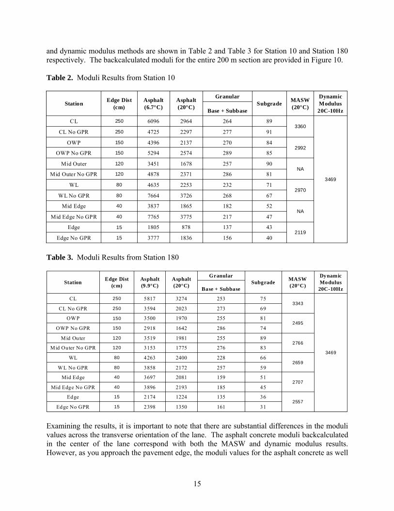
  15

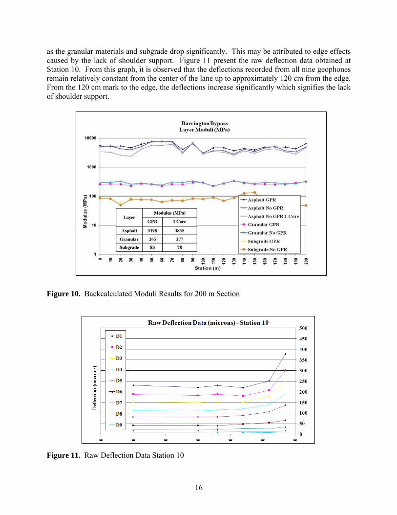
and dynamic modulus methods are shown in Table 2 and Table 3 for Station 10 and Station 180 respectively. The backcalculated moduli for the entire 200 m section are provided in Figure 10. Table 2. Moduli Results from Station 10

401561836377715Edge No GPR2119

43137878180515Edge

472173775776540Mid Edge No GPRNA

521821865383740Mid Edge

672683726766480WL No GPR2970

712322253463580WL

8128623714878120Mid Outer No GPRNA

9025716783451120Mid Outer

8528925745294150OWP No GPR2992

8427021374396150OWP

9127722974725250CL No GPR

3469

33608926429646096250CL

Base + Subbase

Dynamic Modulus

20C-10Hz

MASW (20°C) Subgrade

GranularAsphalt (20°C)

Asphalt (6.7°C)

Edge Dist (cm)Station

401561836377715Edge No GPR2119

43137878180515Edge

472173775776540Mid Edge No GPRNA

521821865383740Mid Edge

672683726766480WL No GPR2970

712322253463580WL

8128623714878120Mid Outer No GPRNA

9025716783451120Mid Outer

8528925745294150OWP No GPR2992

8427021374396150OWP

9127722974725250CL No GPR

3469

33608926429646096250CL

Base + Subbase

Dynamic Modulus

20C-10Hz

MASW (20°C) Subgrade

GranularAsphalt (20°C)

Asphalt (6.7°C)

Edge Dist (cm)Station

Table 3. Moduli Results from Station 180

311611350239815Edge No GPR2557

361351224217415Edge

451852193389640Mid Edge No GPR2707

511592081369740Mid Edge

592572172385880W L No GPR2659

662282400426380WL

8327617753153120Mid Outer No GPR2766

8925519813519120Mid Outer

7428616422918150OWP No GPR2495

8125519703500150OWP

6927320233594250CL No GPR

3469

33437525332745817250CL

Base + Subbase

Dynamic Modulus

20C-10Hz

MASW (20°C)Subgrade

GranularAsphalt (20°C)

Asphalt (9 .9°C)

Edge Dist (cm)Station

311611350239815Edge No GPR2557

361351224217415Edge

451852193389640Mid Edge No GPR2707

511592081369740Mid Edge

592572172385880W L No GPR2659

662282400426380WL

8327617753153120Mid Outer No GPR2766

8925519813519120Mid Outer

7428616422918150OWP No GPR2495

8125519703500150OWP

6927320233594250CL No GPR

3469

33437525332745817250CL

Base + Subbase

Dynamic Modulus

20C-10Hz

MASW (20°C)Subgrade

GranularAsphalt (20°C)

Asphalt (9 .9°C)

Edge Dist (cm)Station

Examining the results, it is important to note that there are substantial differences in the moduli values across the transverse orientation of the lane. The asphalt concrete moduli backcalculated in the center of the lane correspond with both the MASW and dynamic modulus results. However, as you approach the pavement edge, the moduli values for the asphalt concrete as well

  16

as the granular materials and subgrade drop significantly. This may be attributed to edge effects caused by the lack of shoulder support. Figure 11 present the raw deflection data obtained at Station 10. From this graph, it is observed that the deflections recorded from all nine geophones remain relatively constant from the center of the lane up to approximately 120 cm from the edge. From the 120 cm mark to the edge, the deflections increase significantly which signifies the lack of shoulder support. Figure 10. Backcalculated Moduli Results for 200 m Section Figure 11. Raw Deflection Data Station 10

  17

The MASW asphalt modulus only decreases slightly across the lane which could indicate slight amounts of damage in the wheel path, or perhaps construction flaws as you approach the edge (lack of compaction). Consequently, the difference in backcalculated moduli to MASW moduli generally increases near the edge of the lane. The backcalculated moduli are not only influenced by the damage across the traffic lane, but also by the lack of shoulder support. The MASW results are not influenced by the lack of shoulder support as the test focuses solely within the asphalt layer. Therefore the results represent the actual material modulus and not necessarily the modulus required to fit the pavement system. As a result, the MASW modulus may be used to differentiate between edge effects and actual pavement distress. In addition to the variations caused by the edge effects, there are also significant differences between the baclcalculated moduli results obtained with and without GPR thicknesses. The results indicate up to a 40 percent difference in asphalt concrete moduli. Reviewing the data, it should also be noted that the asphalt moduli values incorporating GPR data correspond significantly better with the MASW results, especially at the center lane (no damage or edge effects). Design Parameters To demonstrate the importance of incorporating GPR data into the backcalculation procedure, the modulus and thickness values calculated with and without GPR were used to calculate SNeff based on the 1993 AASHTO Guide for Design of Pavement Structures and remaining service life based on the MEPDG. The AASHTO designs were computed based on equations and methodology provided in the AASHTO Guide. To compute SNeff the 1993 guide specifies two methods. The first method is based on NDT deflection data, while the second uses a visual condition survey assessment and the resultant layer coefficients. However, there are equations and charts found in the guide that enable the computation of layer coefficients based on the existing modulus of the various pavement layers above the subgrade. Utilizing the NDT and condition survey methods, SNeff was calculated for both thickness scenarios for Station 10 and Station 180 as shown in Table 4. The condition survey method was implemented for analyzing the entire 200 m section as shown in Table 5. The difference in SNeff caused by the thickness variation translates into considerable differences in the required overlay thickness. Table 4. SNeff With and Without GPR Thickness Data for Station 10 and Station 180

1.431.757.107.736.707.47180 CL

1.071.596.727.196.397.0910 CL

1.152.207.037.546.577.54180 OWP

1.272.116.977.536.467.3910 OWP

Condition SurveyNDT MethodNo GPRGPRNo GPRGPR

Condition SurveyNDT MethodDifference in Overlay Thickness

(in) Based on SNeff

SNeff

Station

1.431.757.107.736.707.47180 CL

1.071.596.727.196.397.0910 CL

1.152.207.037.546.577.54180 OWP

1.272.116.977.536.467.3910 OWP

Condition SurveyNDT MethodNo GPRGPRNo GPRGPR

Condition SurveyNDT MethodDifference in Overlay Thickness

(in) Based on SNeff

SNeff

Station

  18

Table 5. SNeff With and Without GPR Thickness Data for entire 200 m Section The MEPDG also provides detailed methods to compute remaining service life. These methods are based on asphalt fatigue and subgrade rutting models. The models selected in this research were established by the Asphalt Institute. The number of load repetitions required to cause failure are related to the strain located at critical areas of the pavement structure (bottom of AC layer, top of subgrade). Using moduli values determined from backcalculation and the related thickness values, the strains at these critical areas were determined for both scenarios. An ELSYM 5 spreadsheet was implemented to compute the strains at the bottom of the AC layer and at the top of the subgrade. The results are provided in Table 6. Table 6. Remaining Service Life

9.46.99.38E+074.71E+082.21E+051.63E+051.76E-041.22E-042.11E-042.17E-0423456Average

9.17.48.08E+075.91E+082.14E+051.74E+051.79E-041.15E-042.14E-042.22E-0423456OWP (Edge)

9.56.96.43E+074.53E+082.23E+051.62E+051.89E-041.22E-042.16E-042.27E-0423456OWP (Center)

9.66.51.36E+083.69E+082.25E+051.52E+051.60E-041.28E-042.04E-042.03E-0423456CL

Station 180

6.56.51.39E+083.52E+081.53E+051.53E+051.59E-041.29E-042.18E-042.25E-0423456Average

6.57.01.19E+083.73E+081.52E+051.65E+051.65E-041.27E-042.16E-042.35E-0423456OWP (Edge)

7.47.31.41E+083.39E+081.74E+051.72E+051.59E-041.30E-042.07E-042.18E-0423456OWP (Center)

5.75.21.58E+083.43E+081.35E+051.22E+051.55E-041.30E-042.31E-042.22E-0423456CL

Station 10

No GPRGPRNo GPRGPRNo GPRGPRNo GPRGPRNo GPRGPR

Design Life (Yrs)Nf (Rutting)Nf (Fatigue)Strain in SubgradeStrain in AsphaltESALLocation

9.46.99.38E+074.71E+082.21E+051.63E+051.76E-041.22E-042.11E-042.17E-0423456Average

9.17.48.08E+075.91E+082.14E+051.74E+051.79E-041.15E-042.14E-042.22E-0423456OWP (Edge)

9.56.96.43E+074.53E+082.23E+051.62E+051.89E-041.22E-042.16E-042.27E-0423456OWP (Center)

9.66.51.36E+083.69E+082.25E+051.52E+051.60E-041.28E-042.04E-042.03E-0423456CL

Station 180

6.56.51.39E+083.52E+081.53E+051.53E+051.59E-041.29E-042.18E-042.25E-0423456Average

6.57.01.19E+083.73E+081.52E+051.65E+051.65E-041.27E-042.16E-042.35E-0423456OWP (Edge)

7.47.31.41E+083.39E+081.74E+051.72E+051.59E-041.30E-042.07E-042.18E-0423456OWP (Center)

5.75.21.58E+083.43E+081.35E+051.22E+051.55E-041.30E-042.31E-042.22E-0423456CL

Station 10

No GPRGPRNo GPRGPRNo GPRGPRNo GPRGPRNo GPRGPR

Design Life (Yrs)Nf (Rutting)Nf (Fatigue)Strain in SubgradeStrain in AsphaltESALLocation

The design life provided in Table 6 is calculated based on the fatigue life. From the results, there does not seem to be considerable differences in the design life when considering asphalt fatigue, as the variation in thickness seem to offset the changes in moduli. However, the rutting performance for the GPR data is nearly half of the value from the non GPR results. Because of the low traffic volume, rutting is generally not a concern for this particular section. Consequently, if the thicknesses were smaller and traffic volumes increased, the rutting performance would have a significant effect on the design life.

0.957.197.61Average

No GPRGPR

NDT MethodDifference in

Overlay Thickness (in)

SNeff

Station

0.957.197.61Average

No GPRGPR

NDT MethodDifference in

Overlay Thickness (in)

SNeff

Station

 

  19

CONCLUSIONS Nondestructive deflection testing by means of the FWD in addition to GPR and MASW testing were performed along a 200 meter test section and across the transverse width of the traffic lane to establish variations in thickness and moduli. Cores were also extracted along the test section to calibrate GPR data and to perform dynamic modulus testing for master curve construction. Using GPR, it was determined that a 65 mm variation existed between the center of the lane and the pavement edge. As a result there were also significant differences between the nearest measured core thickness and the actual thickness measured with GPR. Since cores can only be extracted at certain points along a pavement section, GPR results provide a much better estimate to the continuous thickness profile. Consequently, this thickness data can also be used to complement the backcalculation process. It was found that the backcalculated moduli determined with GPR provided a better estimate to the MASW calculated moduli and measured dynamic moduli from conventional methods. In terms of design life and required overlay thickness, there can be significant error if improper thickness and moduli values are incorporated into the analysis. Using the AASHTO 1993 Pavement Guide, the difference in modulus and thickness between GPR and non GPR data in this study resulted in nearly a 2 inch difference in overlay thickness. It was determined that MASW may be used to differentiate between asphalt moduli reductions related to pavement edge effects and actual pavement distress. The MASW results are not influenced by the lack of shoulder support as compared to the backcalculated results. The MASW reduction in modulus across the lane width coincides with actual damage or flaws within the asphalt layer. The backcalculated moduli values show a reduction due to a combination of damage and lack of shoulder support. In addition, the MASW calculated moduli which may be determined to within approximately 20 mm from the surface correspond to the measured dynamic modulus. Consequently, using the MASW determined in-situ moduli values may complement the FWD for thin layer asphalts. REFERENCES Al-Qadi, I.L., and Lahouar, S. (2004). “Ground Penetrating Radar: State of the Practice for

Pavement Assessment”, Materials Evaluation, American Society for Nondestructive Testing, Vol. 62, No. 7, pp. 759-763.

American Association of State Highway and Transportation Officials. (1993). “AASHTO Guide

for Design of Pavement Structures”, Washington, D.C. Barnes, C.L., Trottier, J.-F. (2009-1). “Evaluating High-Frequency Visco-Elastic Moduli in

Asphalt Concrete”, Research in Nondestructive Evaluation, Volume 20, Issue 2, pp.116-130.

Barnes, C.L., Trottier, J.-F. (2009-2). “Hybrid analysis of surface wavefield data from Portland

cement and asphalt concrete plates”, NDT&E International, Volume 42, Issue 2, pp. 106-112.

  20

Heisey, J.S., Stokoe II, K.H., and Meyer, A.H. (1982). “Moduli of pavement systems from spectral analysis of surface waves”, Transportation Research Record 852, Transportation Research Board, National Research Council, Washington, D.C. pp. 22-31.

Irwin, L.H. (2002). “Backcalculation: An Overview and Perspective”,

http://pms.nevadadot.com/2002presentations/11.pdf Jones, R. (1955). “A vibration method for measuring the thickness of concrete road slabs in

situ”, Magazine of Concrete Research, Vol 7, N0. 20., pp.97-102. Loizos, A., and Plati, C. (2007). “Accuracy of pavement thickness estimation using different

ground penetrating radar analysis approaches”, NDT & E International, Elsevier Science, Vol. 40, No. 2, pp. 147-157.

Maser, K.R., Holland, T.J., Roberts, R., and Popovics, J. (2006). “NDE methods for quality

assurance of new pavement thickness”, The International Journal of Pavement Engineering, Vol. 7, No. 1, pp. 1-10.

National Cooperative Highway Research Program (NCHRP) (2004). “NCHRP 1-37A Design

Guide”, Washington, D.C., http:www.trb.org/mepdg/guide.htm. Nazarian, S., Stokoe II, K. H., Hudson, W.R. (1983). “Use of Spectral Analysis of Surface

Waves Method for Determination of Moduli and Thicknesses of Pavement Systems”, Transportation Research Record 930, Transportation Research Board, National Research Council, Washington, D.C. pp. 38-45.

Park, C.B., Miller, R.D., and Xia, J. (1998). “Imaging dispersion curves of surface waves on

multi-channel record”, Kansas Geological Survey, 68th Annual International Meeting of the Society of Exploration Geophysicists, Expanded Abstracts, p. 1377-1380.

Park, C.B., Miller, R.D., and Xia, J. (1999). “Multimodal analysis of high frequency surface

waves”, Proceedings of the Symposium of Applied Geophysics in Engineering and Environmental Problems (SAGEEP 1999), Oakland, CA, p.115-121.

Park, D., Buch, N., Chatti, K. (2001). “Effective Layer Temperature Prediction Model and

Temperature Correction via Falling Weight Deflectometer Deflections”, Transportation Research Record 1764, Transportation Research Board, National Research Council, Washington, D.C. pp. 97-111.

Pellinen, T.K., Witczak, M.W., and Bonaquist, R.A. (2004). “Asphalt mix master curve

construction using sigmoidal fitting function with non-linear least squares optimization”, Recent Advances in Materials Characterization and Modeling of Pavement Systems, American Society of Civil Engineers Geotechnical Special Publication No. 123. pp. 83-101.

  21

Ryden, N., Ulriksen, P., Park, C.B., Miller, R.D., Xia, J., and Ivanov, J. (2001). “High frequency MASW for non-destructive testing of pavements-accelerometer approach”, Proceedings of the Symposium on the Application of Geophysics to Engineering and Environmental Problems (SAGEEP 2001), Environmental and Engineering Geophysical Society, Annual Meeting, Denver, RBA-5.

Ryden, N., Park, C.B., Ulriksen, P., and Miller R.D. (2003). “Lamb wave analysis for non-

destructive testing of concrete plate structures ”, Proceedings of the Symposium on the Application of Geophysics to Engineering and Environmental Problems (SAGEEP 2003), San Antonio, TX April 6-10,INF03.

Ryden, N., Park, C.B., Ulriksen, P., and Miller, R.D. (2004). “Multimodal Approach to Seismic

Pavement Testing”, Journal of Geotechnical and Geoenvironmental Engineering., Vol. 130, No. 6, pp. 636-645.

Ryden, N., Park, C.B. (2006). “Fast simulated annealing inversion of surface waves on pavement

using phase-velocity spectra”, Geophysics, Vol 71, No. 4, pp. R49-R58. Shahin, M. (1994). “Pavement Management for Airports, Roads, and Parking Lots, 2nd Edition”,

Springer, New York, N.Y. Ullidtz, P., and Stubstad, R.N. (1985). Analytical Empirical Pavement Evaluation Using the

Falling Weight Deflectometer”, Transportation Research Record 1022, Transportation Research Board, National Research Council, Washington, D.C. pp. 36-44.

Willett, D.A., Mahboub, K., and Rister, B. (2006). “Accuracy of Ground-Penetrating Radar for

Pavement Layer Thickness Analysis”, Journal of Transportation Engineering, ASCE, Vol. 132, No. 1, pp. 96-103.

Witczak, M.W., and Bari, J. (2004). “Development of a E* master curve database for lime

Modified Asphaltic Mixtures”,http://www.lime.org/Publications/MstrCurve.pdf