Use of Combined System Dependability and Software Reliability Growth ModelsMyron Hecht, Herb Hecht, and Xuegao An

SoHaR Incorporated

www.sohar.com • 8421 Wilshire, Suite 201, • Beverly Hills, CA 90211

[myron, herb, xuegao]@sohar.com

keywords: dependability modeling, reliability growth, software reliability, air traffic control, CASRE, MEADEP

AbstractThis paper describes how MEADEP, a system leveldependability prediction tool, and CASRE, a software reliabilitygrowth prediction tool can be used together to predict systemreliability (probability of failure in a given time interval),availability (proportion of time service is available), andperformability (reward-weighted availability) for a. The systemincludes COTS hardware, COTS software, radar, andcommunication gateways. The performability metric alsoaccounts for capacity changes as processors in a cluster fail andrecover. The Littlewood Verrall and Geometric model is used topredict reliability growth from software test data This predictionis integrated into a system level Markov model that incorporateshardware failures and recoveries, redundancy, coverage failures,and capacity. The results of the combined model can be used topredict the contribution of additional testing upon availabilityand a variety of other figures of merit that support managementdecisions.

1 IntroductionThis paper addresses a new approach for assessment of complexdistributed real time systems used in mission critical or safetycritical applications. We demonstrate the combined use oftraditional system reliability assessment techniques withsoftware reliability growth models to enable the prediction ofwhether such systems will meet their reliability and availabilityrequirements, and demonstrate how such an integrated modelcan be used for system level tradeoffs (e.g., redundancy vs. testtime). Successive generations of both system and softwarereliability prediction methods and tools have been developedsince the early 1970s. However, these techniques assumed thatthe software executed in a single module or node[Schneidewind96] and are therefore not sufficient to address theneeds of current complex systems. By “complex systems”, wemean systems that incorporate both COTS and developmentalsoftware, COTS hardware, and Internet Wide Area Networks(WANs), all of which contribute to system downtime.

Software reliability growth models use measured time betweenerror reports or number of error reports in a time interval. Inmost cases, they evaluate the reduction in failure frequencyduring successive developmental test intervals to estimate thesoftware reliability at the conclusion of a time period. Examples

are the Schneidewind model, the generalized exponential model,the Musa/Okumoto Logarithmic Poisson model, and theLittlewood/Verrall model [ANSI92]. The primary limitation ofreliability growth models is their lack of ability to model systemarchitectures. Because information systems commonlyincorporate parallelism, redundancy, and networks, thereliability of the system cannot be quantified solely by thefailure rate calculated at the software module level. Forexample, several studies have shown that 80 to 95 percent ofsoftware failures in real-time systems are recoverable byredundant processes [Lee93, Tang95]. In such cases, softwarereliability growth models do not provide meaningful answers.

System reliability models use stochastic analysis andcombinatorial probabilistic techniques to predict reliability. Theunderlying assumption in these measurement-based approachesis that the fundamental failure mechanisms are triggeredstochastically, i.e., are non-deterministic (“Heisenbugs”). Themost common modeling techniques are Markov chains andreliability block diagrams. Such models have been used toevaluate operational software based on failure data collectedfrom commercial computer operating systems for more than adecade [Hsueh87, Tang92, Lee93]. Research on estimatingparameters for such models, including failure rates andrestoration times of both hardware and software components,been a research topic in computer engineering for 15 years[Iyer93]. System availability modeling has been used toevaluate availability for air traffic control software systems[Tang95, Tang99, Rosin99] and most recently also to the earlyoperational phase at multiple sites. The problem with systemreliability models is that they do not account for reliabilitygrowth. Thus, they can be used to assess system dependability,but not to predict such dependability during the development andtesting phases.

In this paper, we demonstrate how software and systemreliability models can be integrated to provide a basis forpredicting system availability and to enable business or projectmanagement decisions. Examples of questions that suchmodeling can answer include:

• Given a known cost of downtime and current test data, whatis the economically optimal point at which to stop testing?What uptime benefit will be achieved by additional testingbeyond this point?

• Based on current testing results, what is the highest systemavailability that is likely to be achieved?

• How much more testing will be necessary in order for thesystem to achieve the required availability?

• Is testing or additional redundancy a better strategy forachieving availability goals?

In this paper, we will describe the application of an integratedsystem/software reliability growth model for an Internet web siteserver subsystem. We will then demonstrate how the impact oftest time against capacity and availability can be assessed.Finally, we will demonstrate that substantive economic decisionson test strategies and stopping criteria can be developed usingsuch a model.

The system reliability is assessed in the following examplesusing MEADEP [SoHaR00], a graphically oriented hierarchicalreliability modeling tool. The software reliability prediction toolis SMERFS [Farr93], a well known and widely acceptedsoftware application for evaluation of test data for failure rateand defect discovery rate prediction.

2 Air Traffic Control System ExampleTo demonstrate the principle of the combined model, we will usea simplified system configuration based on the StandardTerminal Automation Replacement System (STARS) now beingdeveloped by the Federal Aviation Administration for upgradesat large airports or complexes of airports. Figure 1 shows theoverall system.

Digitized radar data arrives over telephonelines and is distributed to twoCommunication Gateway subsystems to aprimary system, designated the FullSystem :Level(FSL), and a backupsubsystem, designated as the EmergencyService Level (ESL). Both the FSL andESL use dual redundant switched 100MBPS Ethernet backbones. Allprocessors on the network use middlewareprovided in the Network Services (NWS)

software for status reporting, registration, remote management,and related functions necessaryu for high availability. In theFSL, the data are processed by a server with redundancy runninga Radar Data Processor (RDP) application that performs radardata tracking and correlation. The RDP data are then distributedto the Terminal Controller Workstations (TCWs) or largerTerminal Display Workstations (TDWs) where they aretranslated into a situation display. In the ESL, each workstationperforms its own tracking and correlation along with thesituation display; there is no central RDP server. Systemmanagement is performed through other Monitor and ControlWorkstations (MCWs) running the System Monitor and Control(SMC) software. Other functions that support the primarymission include Data Recording and Playback (DRP) which isperformed on another set of servers on the FCS network and asupport subsystem performs provides site support such assimulation for test and training, adaptation edits for maps andminimum safe altitude warnings. The “P” and “R”, and “FW”designations on the diagram stand for printers, routers, andfirewalls respectively.

3 Dependability ModelThe dependability model for this system involves both thedeveloped software and Commercial off the Shelf (COTS)hardware and software. Developed software undergoes testingand failure removal; its reliability growth is predicted using oneof many reliability growth models, in the Computer AidedSoftware Reliabilty Estimation (CASRE) software packagedeveloped at JPL [Nikora94]. COTS components – whetherhardware or software – have constant failure rates. We have

explained above why suchfailures are primarilyrandom in nature and havefailure rates that can bemeasured using wellestablished techniques thathave been incorporated intothe Measurement BasedDependability (MEADEP ).software developed bySoHaR [Hecht97].

MEADEP creates modelshierarchically. A total of 11submodels were created asshown in Figure 2. The top

CG ProcHW/SWMarkov

CG SubsystemMarkov

RDP ProcHW/SWMarkov

RDP SubsystemMarkov

EthernetMarkov

WkstnHW/SWMarkov

Controller WkstnMarkov

FSLBlock Dgm

ESL WkstnMarkov

ESLMarkov

STARS ModelMarkov

Figure 2. Model hierarchy

ARTCC

Emergency Service Network (100 Mbps)

MSU

PrimaryLinks

M S U

BackupLinks

CommunicationGateway

Radars

M S U

ETMS

CommunicationGateway

R D P DRF SIM

TCW T D W Cert.TCW MCW

R

Full Service Network (100 Mbps)

SSS

R

GPW

P R FW

O S FSCSCOCC

RemoteTowers

R

AIG

Future InterfacesSupport Subsystem

AutomationSubsystem

Figure 1. STARS Top Level System Diagram

level diagram accounts for both the ESL and FSL integrated toprovide the terminal situation display service. Within the FSL,there are submodels for each of the four major subsystems(Communications Gateway, Radar Data Processing, Network,and Controller Workstation). The ESL model is simpler,consisting only of software. With the exception of the Ethernet,which has no software, the other subsystems include bothhardware, COTS software,. and developed software as will bedescribed below. Figure 1 shows a Markov model of the radardata processing server in order to demonstrate the integration ofreliability growth and stochastic reliability models. The systemis available if functional in either the FSL or ESL states. It willfail if a common cause failure (power, network, massive security

failure, etc.) brings down the entire system.

Due to length considerations, we will not consider all of thesubmodels. However, in order to demonstrate the integration of

reliability growth and system level modeling, we will show theRadar Data Processor subsystem (RDP) the ESL workstations.

Figure 4 shows the Radar Data Processing submodel. It is astandard Markov dual redundant model in which state S0represents all processors up, S1 represents one processor downand the other successfully taking over, and Sf represents bothprocessors failed. It is not certain that after a single processorfailure, the second processor will successfully recover, andhence, the probably of successful detection and recovery isrepresented by the variable cRDP.

Figure 5 shows the detailed model of the software and hardwarewithin the radar data processor. There are two primary failuremode categories: hardware and software. These categories areso defined because the recovery time from hardware failures is

assumed to be twice as long (1 hour) as the recovery time fromsoftware failures.

The software failure rate transition is of the greatest interest inthis model. Itg includes terms for the operating system failurerate and the failure rate of the radar data processing applicationsoftware. The failure rate for the application software isexpressed in terms of two intermediate constants, k4 and k5,which are related to the Geometric distribution [Farr96], whichhas the form

1)exp()exp(

+=

βββ

λtesttDD

Equation 1

The constants D and β are calculated from the CASRE toolwhich is in turn based on algorithms developed for the SMERFS[Farr83] software. The geometric model was chosen on thebasis of a best fit for the developmental data used in thisexample.

In Figure 5, there are three states in the model: normal,

SW_failed (any of the major components of the RDP hassuffered a failure resulting in the loss of service), and HW_failed(server hardware failure). The numbers below the state namerepresent rewards, i.e., the value of the state. A reward of 1

ìFSL+ìESL

ëcommon

ëFSL

ëESL

ìFSL

ëFSL

ìESL

ëESL Failed0

FSL

1

ESL1

Normal1

Figure 3. Top Level Markov Model

cRDP*ëRDP

ìRDP

(1-cRDP)*ëRDP

ëRDPìRDP

Sf0

S11

S01

Figure 4. Radar Data Processor Submodel

ìSW

ëOS+k4/(k5+testtime_RDP+1)

ìHW

ëHW

SW_Fail

0

HW_Fail0

Normal

1

. Figure 5. Individual Radar Data Processing

Figure 6 . Geometric and LIttlewood VerrallModel fit for RDP sample data

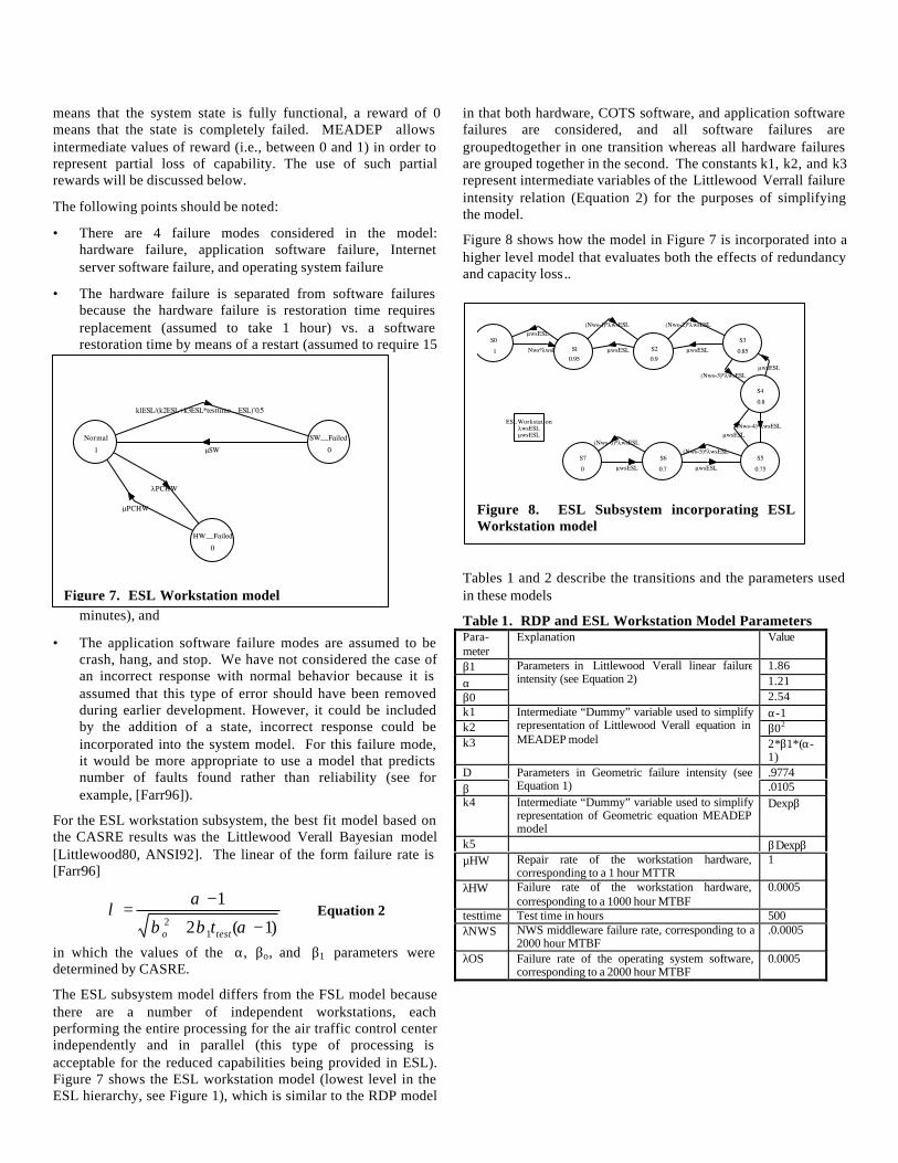
means that the system state is fully functional, a reward of 0means that the state is completely failed. MEADEP allowsintermediate values of reward (i.e., between 0 and 1) in order torepresent partial loss of capability. The use of such partialrewards will be discussed below.

The following points should be noted:

• There are 4 failure modes considered in the model:hardware failure, application software failure, Internetserver software failure, and operating system failure

• The hardware failure is separated from software failuresbecause the hardware failure is restoration time requiresreplacement (assumed to take 1 hour) vs. a softwarerestoration time by means of a restart (assumed to require 15

minutes), and

• The application software failure modes are assumed to becrash, hang, and stop. We have not considered the case ofan incorrect response with normal behavior because it isassumed that this type of error should have been removedduring earlier development. However, it could be includedby the addition of a state, incorrect response could beincorporated into the system model. For this failure mode,it would be more appropriate to use a model that predictsnumber of faults found rather than reliability (see forexample, [Farr96]).

For the ESL workstation subsystem, the best fit model based onthe CASRE results was the Littlewood Verall Bayesian model[Littlewood80, ANSI92]. The linear of the form failure rate is[Farr96]

)1(2

1

12 −+

−=

αββ

αλ

testo tEquation 2

in which the values of the α, βo, and β1 parameters weredetermined by CASRE.

The ESL subsystem model differs from the FSL model becausethere are a number of independent workstations, eachperforming the entire processing for the air traffic control centerindependently and in parallel (this type of processing isacceptable for the reduced capabilities being provided in ESL).Figure 7 shows the ESL workstation model (lowest level in theESL hierarchy, see Figure 1), which is similar to the RDP model

in that both hardware, COTS software, and application softwarefailures are considered, and all software failures aregroupedtogether in one transition whereas all hardware failuresare grouped together in the second. The constants k1, k2, and k3represent intermediate variables of the Littlewood Verrall failureintensity relation (Equation 2) for the purposes of simplifyingthe model.

Figure 8 shows how the model in Figure 7 is incorporated into ahigher level model that evaluates both the effects of redundancyand capacity loss..

Tables 1 and 2 describe the transitions and the parameters usedin these models

Table 1. RDP and ESL Workstation Model ParametersPara-meter

Explanation Value

β1 1.86α 1.21β0

Parameters in Littlewood Verall linear failureintensity (see Equation 2)

2.54k1 α-1k2 β02

k3

Intermediate “Dummy” variable used to simplifyrepresentation of Littlewood Verall equation inMEADEP model 2*β1*(α-

1)D .9774β

Parameters in Geometric failure intensity (seeEquation 1) .0105

k4 Intermediate “Dummy” variable used to simplifyrepresentation of Geometric equation MEADEPmodel

Dexpβ

k5 βDexpβµHW Repair rate of the workstation hardware,

corresponding to a 1 hour MTTR1

λHW Failure rate of the workstation hardware,corresponding to a 1000 hour MTBF

0.0005

testtime Test time in hours 500λNWS NWS middleware failure rate, corresponding to a

2000 hour MTBF.0.0005

λOS Failure rate of the operating system software,corresponding to a 2000 hour MTBF

0.0005

ìPCHW

ëPCHW

HW_Failed0

ìSW

k1ESL/(k2ESL+k3ESL*testtime_ESL)^0.5

SW_Failed0

Normal1

Figure 7. ESL Workstation model

ESLWorkstationëwsESLìwsESL

ìwsESL

(Nws-6)*ëwsESL

ìwsESL

(Nws-5)*ëwsESL

ìwsESL(Nws-4)*ëwsESL

ìwsESL

(Nws-2)*ëwsESL

(Nws-3)*ëwsESL

ìwsESL ìwsESL

S7

0

S6

0.7

S5

0.75

S4

0.8

S3

0.85

(Nws-1)*ëwsESL

S20.9

ìwsESL

Nws*ëwsESL S10.95

S0

1

Figure 8. ESL Subsystem incorporating ESLWorkstation model

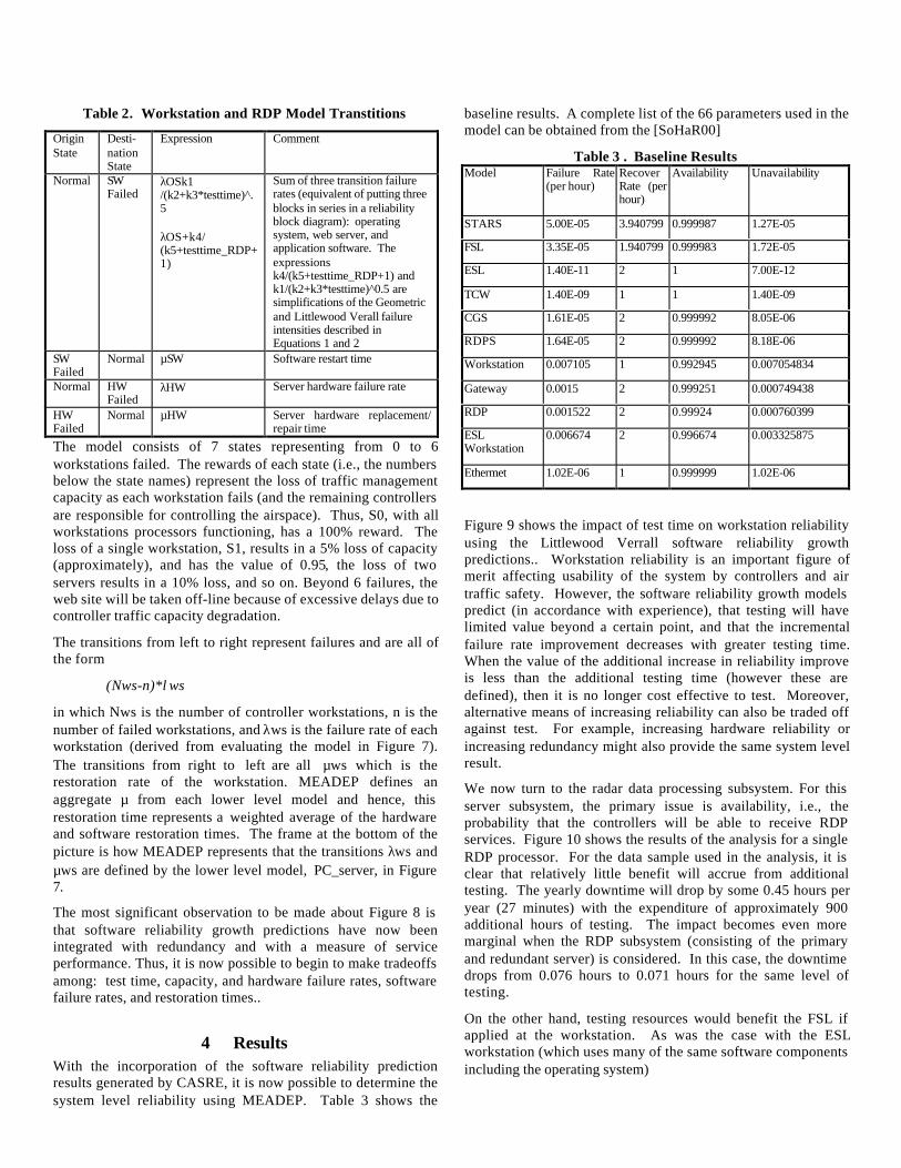
Table 2. Workstation and RDP Model Transtitions

OriginState

Desti-nationState

Expression Comment

Normal SWFailed

λOSk1/(k2+k3*testtime)^.5

λOS+k4/(k5+testtime_RDP+1)

Sum of three transition failurerates (equivalent of putting threeblocks in series in a reliabilityblock diagram): operatingsystem, web server, andapplication software. Theexpressionsk4/(k5+testtime_RDP+1) andk1/(k2+k3*testtime)^0.5 aresimplifications of the Geometricand Littlewood Verall failureintensities described inEquations 1 and 2

SWFailed

Normal µSW Software restart time

Normal HWFailed

λHW Server hardware failure rate

HWFailed

Normal µHW Server hardware replacement/repair time

The model consists of 7 states representing from 0 to 6workstations failed. The rewards of each state (i.e., the numbersbelow the state names) represent the loss of traffic managementcapacity as each workstation fails (and the remaining controllersare responsible for controlling the airspace). Thus, S0, with allworkstations processors functioning, has a 100% reward. Theloss of a single workstation, S1, results in a 5% loss of capacity(approximately), and has the value of 0.95, the loss of twoservers results in a 10% loss, and so on. Beyond 6 failures, theweb site will be taken off-line because of excessive delays due tocontroller traffic capacity degradation.

The transitions from left to right represent failures and are all ofthe form

(Nws-n)*λws

in which Nws is the number of controller workstations, n is thenumber of failed workstations, and λws is the failure rate of eachworkstation (derived from evaluating the model in Figure 7).The transitions from right to left are all µws which is therestoration rate of the workstation. MEADEP defines anaggregate µ from each lower level model and hence, thisrestoration time represents a weighted average of the hardwareand software restoration times. The frame at the bottom of thepicture is how MEADEP represents that the transitions λws andµws are defined by the lower level model, PC_server, in Figure7.

The most significant observation to be made about Figure 8 isthat software reliability growth predictions have now beenintegrated with redundancy and with a measure of serviceperformance. Thus, it is now possible to begin to make tradeoffsamong: test time, capacity, and hardware failure rates, softwarefailure rates, and restoration times..

4 ResultsWith the incorporation of the software reliability predictionresults generated by CASRE, it is now possible to determine thesystem level reliability using MEADEP. Table 3 shows the

baseline results. A complete list of the 66 parameters used in themodel can be obtained from the [SoHaR00]

Table 3 . Baseline ResultsModel Failure Rate

(per hour)RecoverRate (perhour)

Availability Unavailability

STARS 5.00E-05 3.940799 0.999987 1.27E-05

FSL 3.35E-05 1.940799 0.999983 1.72E-05

ESL 1.40E-11 2 1 7.00E-12

TCW 1.40E-09 1 1 1.40E-09

CGS 1.61E-05 2 0.999992 8.05E-06

RDPS 1.64E-05 2 0.999992 8.18E-06

Workstation 0.007105 1 0.992945 0.007054834

Gateway 0.0015 2 0.999251 0.000749438

RDP 0.001522 2 0.99924 0.000760399

ESLWorkstation

0.006674 2 0.996674 0.003325875

Ethermet 1.02E-06 1 0.999999 1.02E-06

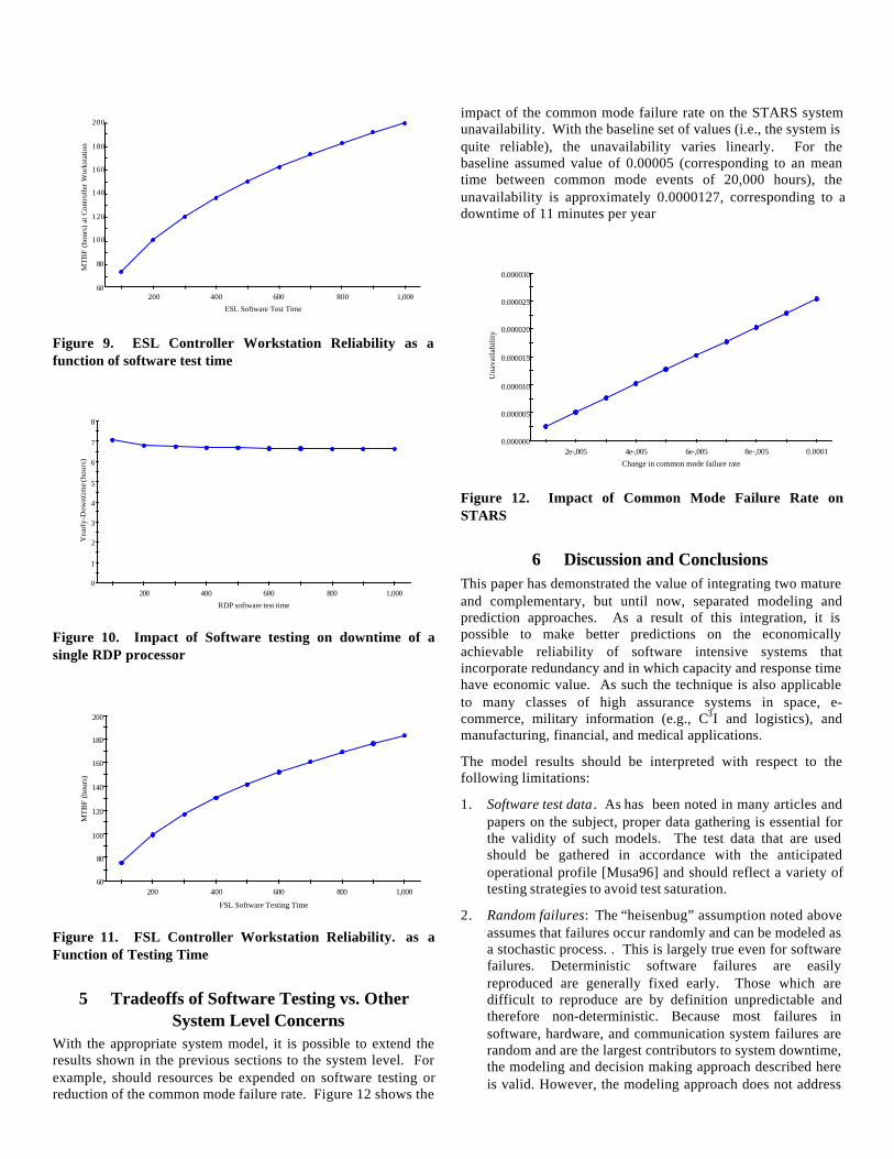
Figure 9 shows the impact of test time on workstation reliabilityusing the Littlewood Verrall software reliability growthpredictions.. Workstation reliability is an important figure ofmerit affecting usability of the system by controllers and airtraffic safety. However, the software reliability growth modelspredict (in accordance with experience), that testing will havelimited value beyond a certain point, and that the incrementalfailure rate improvement decreases with greater testing time.When the value of the additional increase in reliability improveis less than the additional testing time (however these aredefined), then it is no longer cost effective to test. Moreover,alternative means of increasing reliability can also be traded offagainst test. For example, increasing hardware reliability orincreasing redundancy might also provide the same system levelresult.

We now turn to the radar data processing subsystem. For thisserver subsystem, the primary issue is availability, i.e., theprobability that the controllers will be able to receive RDPservices. Figure 10 shows the results of the analysis for a singleRDP processor. For the data sample used in the analysis, it isclear that relatively little benefit will accrue from additionaltesting. The yearly downtime will drop by some 0.45 hours peryear (27 minutes) with the expenditure of approximately 900additional hours of testing. The impact becomes even moremarginal when the RDP subsystem (consisting of the primaryand redundant server) is considered. In this case, the downtimedrops from 0.076 hours to 0.071 hours for the same level oftesting.

On the other hand, testing resources would benefit the FSL ifapplied at the workstation. As was the case with the ESLworkstation (which uses many of the same software componentsincluding the operating system)

60

80

100

120

140

160

180

200

200 400 600 800 1,000

MT

BF

(hou

rs)

at C

ontr

olle

r W

orks

tatio

n

ESL Software Test Time

Figure 9. ESL Controller Workstation Reliability as afunction of software test time

0

1

2

3

4

5

6

7

8

200 400 600 800 1,000

Yea

rly-

Dow

ntim

e (ho

urs)

RDP software test time

Figure 10. Impact of Software testing on downtime of asingle RDP processor

60

80

100

120

140

160

180

200

200 400 600 800 1,000

MTB

F (h

ours

)

FSL Software Testing Time

Figure 11. FSL Controller Workstation Reliability. as aFunction of Testing Time

5 Tradeoffs of Software Testing vs. OtherSystem Level Concerns

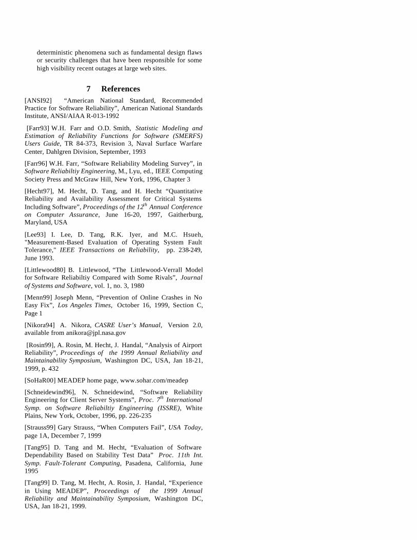
With the appropriate system model, it is possible to extend theresults shown in the previous sections to the system level. Forexample, should resources be expended on software testing orreduction of the common mode failure rate. Figure 12 shows the

impact of the common mode failure rate on the STARS systemunavailability. With the baseline set of values (i.e., the system isquite reliable), the unavailability varies linearly. For thebaseline assumed value of 0.00005 (corresponding to an meantime between common mode events of 20,000 hours), theunavailability is approximately 0.0000127, corresponding to adowntime of 11 minutes per year

0.000000

0.000005

0.000010

0.000015

0.000020

0.000025

0.000030

2e-,005 4e-,005 6e-,005 8e-,005 0.0001

Una

vaila

bilit

y

Change in common mode failure rate

Figure 12. Impact of Common Mode Failure Rate onSTARS

6 Discussion and ConclusionsThis paper has demonstrated the value of integrating two matureand complementary, but until now, separated modeling andprediction approaches. As a result of this integration, it ispossible to make better predictions on the economicallyachievable reliability of software intensive systems thatincorporate redundancy and in which capacity and response timehave economic value. As such the technique is also applicableto many classes of high assurance systems in space, e-commerce, military information (e.g., C3I and logistics), andmanufacturing, financial, and medical applications.

The model results should be interpreted with respect to thefollowing limitations:

1. Software test data . As has been noted in many articles andpapers on the subject, proper data gathering is essential forthe validity of such models. The test data that are usedshould be gathered in accordance with the anticipatedoperational profile [Musa96] and should reflect a variety oftesting strategies to avoid test saturation.

2. Random failures: The “heisenbug” assumption noted aboveassumes that failures occur randomly and can be modeled asa stochastic process. . This is largely true even for softwarefailures. Deterministic software failures are easilyreproduced are generally fixed early. Those which aredifficult to reproduce are by definition unpredictable andtherefore non-deterministic. Because most failures insoftware, hardware, and communication system failures arerandom and are the largest contributors to system downtime,the modeling and decision making approach described hereis valid. However, the modeling approach does not address

deterministic phenomena such as fundamental design flawsor security challenges that have been responsible for somehigh visibility recent outages at large web sites.

7 References[ANSI92] “American National Standard, RecommendedPractice for Software Reliability”, American National StandardsInstitute, ANSI/AIAA R-013-1992

[Farr93] W.H. Farr and O.D. Smith, Statistic Modeling andEstimation of Reliability Functions for Software (SMERFS)Users Guide, TR 84-373, Revision 3, Naval Surface WarfareCenter, Dahlgren Division, September, 1993

[Farr96] W.H. Farr, “Software Reliability Modeling Survey”, inSoftware Reliabiltiy Engineering, M., Lyu, ed., IEEE ComputingSociety Press and McGraw Hill, New York, 1996, Chapter 3

[Hecht97], M. Hecht, D. Tang, and H. Hecht “QuantitativeReliability and Availability Assessment for Critical SystemsIncluding Software”, Proceedings of the 12th Annual Conferenceon Computer Assurance, June 16-20, 1997, Gaitherburg,Maryland, USA

[Lee93] I. Lee, D. Tang, R.K. Iyer, and M.C. Hsueh,"Measurement-Based Evaluation of Operating System FaultTolerance," IEEE Transactions on Reliability, pp. 238-249,June 1993.

[Littlewood80] B. Littlewood, “The Littlewood-Verrall Modelfor Software Reliabiltiy Compared with Some Rivals”, Journalof Systems and Software, vol. 1, no. 3, 1980

[Menn99] Joseph Menn, “Prevention of Online Crashes in NoEasy Fix”, Los Angeles Times, October 16, 1999, Section C,Page 1

[Nikora94] A. Nikora, CASRE User’s Manual, Version 2.0,available from anikora@jpl.nasa.gov

[Rosin99], A. Rosin, M. Hecht, J. Handal, “Analysis of AirportReliability”, Proceedings of the 1999 Annual Reliability andMaintainability Symposium, Washington DC, USA, Jan 18-21,1999, p. 432

[SoHaR00] MEADEP home page, www.sohar.com/meadep

[Schneidewind96], N. Schneidewind, “Software ReliabilityEngineering for Client Server Systems”, Proc. 7th InternationalSymp. on Software Reliabiltiy Engineering (ISSRE), WhitePlains, New York, October, 1996, pp. 226-235

[Strauss99] Gary Strauss, “When Computers Fail”, USA Today,page 1A, December 7, 1999

[Tang95] D. Tang and M. Hecht, “Evaluation of SoftwareDependability Based on Stability Test Data” Proc. 11th Int.Symp. Fault-Tolerant Computing, Pasadena, California, June1995

[Tang99] D. Tang, M. Hecht, A. Rosin, J. Handal, “Experiencein Using MEADEP”, Proceedings of the 1999 AnnualReliability and Maintainability Symposium, Washington DC,USA, Jan 18-21, 1999.