Embed Size (px)
Citation preview

USE OF AN EVAPOTRANSPIRATION MODEL AND A GEOGRAPHIC INFORMATION SYSTEM (GIS) TO ESTIMATE THE
IRRIGATION POTENTIAL OF THE TRASVASE SYSTEM IN THE SANTA ELENA PENINSULA,
GUAYAS, ECUADOR
By
CAMILO CORNEJO
A THESIS PRESENTED TO THE GRADUATE SCHOOL OF THE UNIVERSITY OF FLORIDA IN PARTIAL FULFILLMENT
OF THE REQUIREMENTS FOR THE DEGREE OF MASTER OF SCIENCE
UNIVERSITY OF FLORIDA
2003

To my Family

ACKNOWLEDGMENTS
This thesis work would not have been completed without the help of several people
whom I wish to thank. First, I thank my advisor Dr. Dorota Z. Haman for all her help and
support, interest, knowledge, problem solving and advice. Thanks go to my supervisory
committee, whose comments and edits contribute substantially to my research and to this
document. I would also like to thank to thank to all the people from ESPOL and
CEDEGE in Guayaquil, Ecuador for helping me whenever I needed information for my
research. Special thanks go to my friends, who always help me when needed. Finally, I
would like to thank the very special people in my life, my girlfriend and my family, for
their support.
iii

TABLE OF CONTENTS page ACKNOWLEDGMENTS ................................................................................................. iii
LIST OF TABLES............................................................................................................ vii
LIST OF FIGURES .............................................................................................................x
LIST OF OBJECTS ......................................................................................................... xiii
LIST OF ABBREVIATIONS.......................................................................................... xiv
ABSTRACT.......................................................................................................................xv
CHAPTER 1 LITERATURE REVIEW .............................................................................................1
Significance of Irrigation in Agriculture ......................................................................1 Reference Evapotranspiration.......................................................................................3 Use of FAO Penman-Monteith to Estimate Reference Evapotranspiration .................4 Actual Crop Evapotranspiration ...................................................................................5 Computerized Crop Water Use Simulations.................................................................5 Irrigation Efficiency......................................................................................................7 Irrigation Techniques..................................................................................................10 Application of GIS to Irrigation Management............................................................11 GIS Data Quality Analysis .........................................................................................12 Perceptions about Irrigation........................................................................................15
2 INTRODUCTION AND PROJECT AREA REVIEW ..............................................17
Introduction.................................................................................................................17 Irrigated Area..............................................................................................................17 Agriculture and Irrigation ...........................................................................................19 On-Farm Technologies ...............................................................................................20 Policy ..........................................................................................................................20 Actual Situation and Projections ................................................................................21 Characteristics of the Santa Elena Peninsula..............................................................23 Meteorological Data ...................................................................................................27 Climatic Classifications ..............................................................................................33 Soils ............................................................................................................................36
iv

3 WEATHER DATA ANALYSIS FOR CROPWAT MODEL ...................................39
Weather Stations Distribution.....................................................................................40 Estimating Missing Climatic Data..............................................................................41 Estimating Weather Data Sets for the Santa Elena Peninsula ....................................45
4 GEOGRAPHIC INFORMATION SISTEM ..............................................................52
Introduction.................................................................................................................52 Mapping Systems........................................................................................................54 ArcGIS........................................................................................................................55 Original Maps .............................................................................................................56 Data Quality Problems with the Santa Elena Peninsula Data Set ..............................59 GIS Layers Created or Edited for the Project from the Original Maps ......................65 Creation of Evapotranspiration Surface Maps............................................................71
5 WATER AVAILABILITY AND ITS USE IN THE SANTA ELENA
PENINSULA ..............................................................................................................74
Infrastructure...............................................................................................................74 TRASVASE Santa Elena............................................................................................74 Water Loss from the Canals and Dams to Evaporation..............................................79 Irrigation Technology used in the Santa Elena Peninsula ..........................................82 Water Consumption ....................................................................................................83 Reference Evapotranspiration Surface Maps..............................................................84 Agricultural Production in the Santa Elena Peninsula................................................91
6 METHODOLOGY .....................................................................................................94
Evapotranspiration......................................................................................................94 Open Water Evaporation ............................................................................................95 Crop Water Requirement ............................................................................................96 Crop Irrigation Requirement.......................................................................................99 Scenarios.....................................................................................................................99
7 RESULTS AND DISCUSSION...............................................................................103
Conclusion ................................................................................................................113 Suggestions for Future Work....................................................................................114
APPENDIX A MAPS .......................................................................................................................116
B AVERAGE WEATHER DATA...............................................................................124
C CROPWAT REFERENCE EVAPOTRANSPIRATION TABLES.........................130
v

D ECOCROP SELECTION CRITERIA TABLES......................................................137
E TROPICAL CROPS .................................................................................................148
F IRRIGATION REQUIREMENTS ...........................................................................167
G PROGRAM TO CALCULATE CROP IRRIGATION REQUIREMENT..............172
LIST OF REFERENCES.................................................................................................175
BIOGRAPHICAL SKETCH ...........................................................................................180
vi

LIST OF TABLES
Table page 1-1 Conveyance efficiency (Ec) .......................................................................................8
1-2 Field application efficiency (Ea) ................................................................................8
2-1 Minor watersheds .....................................................................................................26
2-2 Basins that start in the Coastal Mountain Range......................................................26
2-3 Climate types............................................................................................................34
2-4 Köppen climate classification for the SEP...............................................................35
2-5 Soils ..........................................................................................................................36
3-1 Distances among stations (m) and elevation (mmsl) ...............................................40
3-2 Regression analysis method .....................................................................................48
3-3 Creating new values .................................................................................................49
4-1 Comparison of interpolation methods ......................................................................69
5-1 Main dams ................................................................................................................77
5-2 Approximated surface areas of the canals................................................................80
5-3 Approximated surface areas of the dams .................................................................80
5-4 Canal description......................................................................................................81
5-5 Chongón-Daular-Cerecita pressurized system, Zone I (2001).................................82
5-6 Chongón-Cerecita-Playas canal, Zone I (2001) .......................................................82
5-7 El Azúcar-Río Verde canal, Zone II (2001) .............................................................83
5-8 Crop growing period ................................................................................................85
5-9 Crop coefficients ......................................................................................................89
vii

5-10 Crops planted and projected increase in the Santa Elena Peninsula ........................93
6-1 Chongón-San Isidro, Zone I, crop water requirements (CWR) ..............................97
6-2 San Isidro-Playas, Zone I, crop water requirements (CWR)...................................97
6-3 Chongón-El Azúcar, Zone II, crop water requirements (CWR) .............................98
7-1 Scenario A, Zone II.................................................................................................104
7-2 Scenario A, Zone I .................................................................................................105
7-3 Total area that can be irrigated under different scenarios ......................................106
7-4 Areas that could be irrigated during dry season in the SEP, Scenario A................109
7-5 Areas covered by different buffers of the canals in the SEP ..................................111
7-6 Comparison of areas that could be irrigated according different sources ..............111
B-1 Available weather data sets ....................................................................................124
B-2 Chongón weather station........................................................................................125
B-3 Playas weather station ............................................................................................126
B-4 El Azúcar weather station ......................................................................................127
B-5 San Isidro weather station ......................................................................................128
B-6 Suspiro weather station ..........................................................................................129
C-1 Reference evapotranspiration Chongón .................................................................130
C-2 Reference evapotranspiration El Azúcar................................................................131
C-3 Reference evapotranspiration Playas .....................................................................132
C-4 Reference evapotranspiration San Isidro................................................................133
C-5 Reference evapotranspiration Suspiro....................................................................134
C-6 Open water evaporation values per canal...............................................................136
C-7 Open water evaporation from dams .......................................................................136
F-1 Chongón-San Isidro, 50% efficiency .....................................................................167
F-2 San Isidro-Playas, 50% efficiency .........................................................................167
viii
F-3 Chongón-El Azúcar, 50% efficiency .....................................................................168
F-4 Chongón - San Isidro, 70% efficiency ...................................................................168
F-5 San Isidro-Playas, 70% efficiency .........................................................................169
F-6 Chongón-El Azúcar, 70% efficiency .....................................................................169
F-7 Chongón-San Isidro, 90% efficiency .....................................................................170
F-8 San Isidro-Playas, 90% efficiency .........................................................................170
F-9 Chongón-El Azúcar, 90% efficiency .....................................................................171
ix

LIST OF FIGURES
Figure page 1-1 Dual crop coefficient curve ........................................................................................6
2-1 Canal in construction, TRASVASE Santa Elena .....................................................22
2-2 Landscape of the Santa Elena Peninsula ..................................................................24
2-3 Location of the Santa Elena Peninsula .....................................................................25
2-4 Javita River, an intermittent river at SEP.................................................................25
2-5 Historical average precipitation in the Santa Elena Peninsula .................................31
2-7 Papadakis climate classification...............................................................................34
3-1 Weather stations .......................................................................................................41
3-2 Chongón vs. El Azúcar.............................................................................................51
3-3 Chongón vs. El Suspiro............................................................................................51
3-4 Chongón vs. Playas ..................................................................................................51
4-1 Soil types on Santa Elena Peninsula, original map ..................................................57
4-2 Köppen climate classification of Santa Elena Peninsula .........................................57
4-3 Dams location on Santa Elena Peninsula .................................................................58
4-4 Canals and other features .........................................................................................59
4-5 Errors in the hydrology maps of the SEP.................................................................61
4-6 Overlap error ............................................................................................................63
4-7 Main soil types layer created for the Santa Elena Peninsula....................................65
4-8 Ecological zones.......................................................................................................66
4-9 Canals .......................................................................................................................67
x

4-10 Actual farm locations ...............................................................................................68
4-11 Surface maps of weather data for January................................................................72
5-1 Daule-Peripa Dam ....................................................................................................74
5-2 Hydroelectric plant, ‘Proyecto de Propósito Multiple Jaime Roldós Aguilera’ ......75
5-3 Chongón Dam ..........................................................................................................76
5-4 Daule pumping station .............................................................................................76
5-5 Zone II potabilization plant ......................................................................................78
5-6 Canal.........................................................................................................................78
5-7 Canal San Rafael, TRASVASE project ...................................................................79
5-8 Trapezoidal canal .....................................................................................................81
5-9.1 Average reference evapotranspiration for the SEP I ...............................................86
5-9.2 Average reference evapotranspiration for the SEP II ..............................................87
5-10 Agricultural Production in the Santa Elena Peninsula .............................................92
6-1 Evaporation from canals of the TRASVASE system...............................................96
6-2 Irrigation zones in the Santa Elena Peninsula ........................................................100
7-1 Buffers from the canals in the Santa Elena Peninsula............................................110
A-1 Maximum annual precipitation isohyets ................................................................116
A-2 Minimum annual precipitation isohyets .................................................................117
A-3 Average annual precipitation isohyets ...................................................................118
A-4 Complete map of soils in the Santa Elena Peninsula .............................................119
A-5 Santa Elena farms...................................................................................................120
A-6 Chongón farms .......................................................................................................121
A-7 Cerecita farms ........................................................................................................122
A-8 Azúcar-Rio Verde farms ........................................................................................123
C-1 Surface maps used to create a reference evapotranspiration map ..........................135
xi
E-1 Aloe plantation, Santa Elena Peninsula..................................................................148
E-2 Plantain in the Santa Elena Peninsula ....................................................................152
E-3 Grapes.....................................................................................................................154
E-4 Mangos ...................................................................................................................155
E-5 Onion plantation and onions, Santa Elena Peninsula.............................................157
E-6 Papaya plantation in the Santa Elena Peninsula.....................................................158
G-1 Program to calculate crop irrigation requirement, input table and graph...............173
G-2 Program to calculate crop irrigation requirement, results table .............................174
xii

LIST OF OBJECTS
Objects 1. Program to calculate water requirement in the Santa Elena Peninsula
2. PDF version of the user manual for the water requirement program
3. Microsoft Word 2000 version of the user manual for the water requirement program
xiii

LIST OF ABBREVIATIONS
CEDEGE Commission for the Development of the Guayas River Basin, Ecuador
http://www.cedege.gov.ec
CWR Crop Water Requirement
CIR Crop Irrigation Requirement
ESPOL Polytechnic School of the Littoral, Ecuador http://www.espol.edu.ec
ETo Reference evapotranspiration
ETc Actual evapotranspiration
FAO Food and Agricultural Organization http://www.fao.org
FGDC Federal Geographic Data Committee http://www.fgdc.gov
GIS Geographic Information System
GPS Global Positioning System
IDW Inverse Distance Weighted
IGM Geographic Military Institute, Ecuador http://www.igm.gov.ec
ISO International Organization for Standardization
Kc Crop coefficient
SEP Santa Elena Peninsula
USDA United States Department of Agriculture http://www.usda.gov
WCD World Commission on Dams http://www.dams.org/
xiv

Abstract of Thesis Presented to the Graduate School
of the University of Florida in Partial Fulfillment of the Requirements for the Degree of Master of Science
USE OF AN EVAPOTRANSPIRATION MODEL AND A GEOGRAPHIC INFORMATION SYSTEM (GIS) TO ESTIMATE THE
IRRIGATION POTENTIAL OF THE TRASVASE SYSTEM IN THE SANTA ELENA PENINSULA,
GUAYAS, ECUADOR
By
Camilo Cornejo
May 2003
Chair: Dorota Z. Haman Cochair: Jonathan D. Jordan Major Department: Agricultural and Biological Engineering
Irrigated agriculture produces more than 40 % of the world food supply, using
20 % of the agricultural land in developing countries. Food production is important,
especially in developing countries like Ecuador. The TRASVASE irrigation system was
constructed to provide water for irrigation to the Santa Elena Peninsula in Ecuador.
However, this project performs below expectations. One of the limitations is that the total
area that this irrigation system could irrigate has not been determined. Available
geographic, climatic, and soils and land use data were summarized for the Santa Elena
Peninsula using a Geographic Information System. The total area that can be irrigated
was calculated based on the evapotranspiration concept used by CROPWAT software
from UN/FAO. Evapotranspiration is a sum of the water evaporation from the soil and
plant surfaces, and transpiration from the plant leaves.
xv

Calculation of evapotranspiration uses weather parameters like air temperature,
relative humidity, solar radiation, and wind speed. Taking into consideration the water
used by the potable water treatment plants and the water loss thru evaporation and
seepage from the canals and dams, total water available for irrigation can be calculated.
This total available water divided by the crop water requirement gives the total area that
the TRASVASE system could irrigate. To cover a wide range of possible variations in
irrigation technology and crops planted in the area, nine scenarios were tested. The
variables were three levels of in-field water application efficiency (50 %, 70 %, and
90 %); and three levels of the crop water requirement (high, low, and a mixture of high
and low).
Results of this project show that with an in-field application efficiency of 90 % and
low-water-requirement crops, 15,506 hectares could be irrigated. However, with 50 %
application efficiency and high-water-requirement crops, the area is reduced to 7,700
hectares.
It is obvious that very efficient irrigation technologies must be used in the Santa
Elena Peninsula to optimize the use of water. Good management and maintenance of
those irrigation systems are also needed. Agricultural production has to be planned to
minimize water use and to increase the total area to be irrigated.
xvi

CHAPTER 1 LITERATURE REVIEW
Significance of Irrigation in Agriculture
Irrigation is a process that uses more than two-thirds of the Earth’s renewable water
resources and feeds one-third of the Earth’s population (Stanhill 2002). Some 2.4 billion
people depend directly on irrigated agriculture for food and employment. Irrigated
agriculture thus plays an essential role in meeting the basic needs of billions of people in
developing countries (FAO 1996). Although water resources are still ample on a global
scale, serious water shortages are developing in the arid and semi-arid regions (Hall
1999).
There is a need to focus attention on the growing problem of water scarcity in
relation to food production. The World Food Summit of November 1996, drew attention
to the importance of water as a vital resource for future development (FAO 1996). A
major part of the developed global water resources is used for food production. The
estimated minimum water requirement per capita is 1,200 m3 annually (50m3 for
domestic use and 1,150 m3 for food production) (FAO 1996).
Sustainable food production depends on judicious use of water resources as fresh
water for human consumption and agriculture become increasingly scarce. To meet future
food demands and growing competition for clean water, a more effective use of water in
both irrigated and rainfed agriculture will be essential (Smith 2000). Options to increase
water-use efficiency include harvesting rainfall, reducing irrigation water losses, and
adopting cultural practices that increase production per unit of water.
1

2
Irrigation is an obvious option to increase and stabilize crop production. Major
investments have been made in irrigation over the past 30 years by diverting surface
water and extracting groundwater. The irrigated areas in the world have, over a period of
30 years, increased by 25 % (mainly during a period of accelerated growth in the 1970s
and early 1980s) (FAO 1993).
A major constraint to the understanding of the use of water is the difficulty
associated with its measurement and quantification. Measurement and data collection of
discharge in canals is difficult and fraught with potential errors.
Necessary conditions for the optimal performance of regional water delivery
systems include well-defined water rights; infrastructure capable of providing the service
embodied in the water rights, and assigned responsibilities for all aspects of system
operation (Perry 1995). One or more of those conditions may be missing in some regional
systems at the start of irrigation deliveries. In other systems problems may develop over
time with changes in land ownership, cropping patterns, and the volume of water
available for delivery in the system. Problems with cost recovery and inadequate
maintenance also can reduce the efficiency of regional water-delivery systems.
Water use for crop production is depending on the interaction of climatic
parameters that determine crop evapotranspiration and water supply from rain (Smith
2000). Compilation, processing, and analysis of meteorological information for crop
water use and crop production are therefore key elements in developing strategies to
optimize the use of water for crop production and to introduce effective
water-management practices. Estimating crop water use from climatic data is essential to,
better water-use efficiency.

3
Because most of the Earth’s irrigated land is in the underdeveloped world (where
food, water, and skilled manpower are in short supply), it is important to use the simplest,
cheapest, and most practical meteorological method to improve crop water-use efficiency
in irrigation. Stanhill (2002) says that in these regions use of standard, correctly sited and
maintained evaporation pans operating within a national network can provide the basis
for a scheduling method in which the use of empirical crop coefficients is accepted.
These coefficients reflect the local economic as well as agronomic, climatologic and
hydrological (water quality) situation (Stanhill 2002). However, the literature often
contradicts. Hillel (1997) said: “the use of ‘evaporation pans’ has several shortcomings.”
Smith (2000) stated that agro-meteorology would play a key role in the looming
global water crisis. Appropriate strategies and policies need to be defined, including
strengthening of national use of climatic data for planning and managing of sustainable
agriculture and for drought mitigation.
The limitations of currently available methods for measuring rates of evaporation
from natural and agricultural surfaces are well known; as is the resulting lack of
information (local and global) on this major element in the hydrological cycle. A
practical method (suitable for routine use in meteorological station networks) is to use
calculations based on other meteorological measurements, like those used by the
Penman-Monteith method (Stanhill 2002).
Reference Evapotranspiration
Several definitions of reference evapotranspiration ETo have been formulated.
Jensen (1993) defined ETo as the rate at which water, if available, would be removed
from the soil and plant surface. Pereira et al. (1999) stated that Duke simplified the
definition of ETo to “the water used by a well-watered reference crop, such alfalfa, which

4
fully covers the soil surface.” The modified Penman combination equation is used to
compute ETo, as it is considered to be a satisfactory estimation equation when daily
estimates of ETo are desired (Jensen et al. 1990).
Use of FAO Penman-Monteith to Estimate Reference Evapotranspiration
This approach was introduced by Penman in 1948 to estimate open-water
evaporation (Penman 1948); and extended by Monteith in 1965 to directly estimate
evaporation from vegetation-covered surfaces (Monteith 1965). It is now the
recommended method by the FAO to calculate reference crop evapotranspiration (Allen
et al. 1998).
Studies showed the superior performance of the Penman–Monteith approach, in
both arid and humid climates, and convincingly confirmed the sound underlying concepts
of the method. Based on these findings, the method was recommended by the FAO Panel
of Experts (convened in 1990) for adoption as a new standard for reference crop
evapotranspiration estimates (Hall 1999).
The use of the Penman-Monteith equation in irrigation practice requires empirical
coefficients to modify—in general to reduce but sometimes to increase—the estimates of
reference crop evapotranspiration (Stanhill 2002).
Use of FAO Penman–Monteith with limited climatic data. The limited
availability of the full range of climatic data (particularly data on sunshine, humidity and
wind) has often prevented the use of the combination methods and resulted in the use of
empirical methods (which require only temperature, pan, or radiation data). This has
contributed to the confusing use of different ETo methods and conflicting
evapotranspiration values. To overcome this constraint and to further use of a single
method, additional studies have been undertaken to provide recommendations on the

5
using FAO Penman-Monteith when no humidity, radiation or wind data are available. As
a result, procedures are presented to estimate humidity and radiation from
maximum/minimum temperature data and to adopt global estimates for wind speed. The
availability of worldwide climatic databases further facilitates the adoption of values
from nearby stations. Such procedures have proven to perform better than any of the
alternative empirical formulas; and will largely improve transparency of calculated
evapotranspiration values (Smith et al. 1996).
Actual Crop Evapotranspiration
Procedures for estimating crop evapotranspiration have been well established by
Doorenbos and Pruitt (1977), using a series of recommended crop coefficient values (Kc)
to determine ETcrop (ETc) from reference evapotranspiration (ETo), as follows:
ETc = KcETo (1-1)
This formula represents the single crop coefficient. Crop evapotranspiration (ETc)
refers to evapotranspiration of a disease-free crop, grown in very large fields, not short of
water and fertilizer. Estimation of ETc is essential for computing the soil water balance
and irrigation scheduling. ETc is governed by weather and crop condition (Smith, 2000).
The specific wetting (irrigation) events are taken into account (spikes in Figure 1-1).
Computerized Crop Water Use Simulations
Practical procedures and criteria need to be defined to enhance the introduction and
application of effective water use practices for crop production. The introduction of
computerized procedures linked to digital databases and geographic information systems
(GIS) will greatly enhance the use of appropriate planning and management techniques
for water use in irrigated and rainfed agriculture. Computerized procedures greatly
facilitate the estimation of crop water requirements from climatic data and allow

6
the development of standardized information and criteria for planning and management
of rainfed and irrigated agriculture.
Figure 1-1. Dual crop coefficient curve
Figure 1-1 shows the crop coefficient divided in different stages according to crop
development.
The FAO-CROPWAT program (Smith 1992) incorporates procedures for reference
crop evapotranspiration and crop water requirements and allows the simulation of crop
water use under various climate (CLIMWAT 1994), crop and soil conditions.
As a decision support system CROPWAT’s main functions include: (1) the
calculation of reference evapotranspiration according to the FAO Penman-Monteith
method; (2) crop water requirements using revised crop coefficients (FAO Paper 56,
compared to the data from FAO Paper 49) and crop growth periods; (3) effective rainfall
and irrigation requirements; (4) scheme irrigation water supply for a given cropping
pattern; (5) daily water balance computations (Smith 1992).

7
Irrigation Efficiency
Classical overall irrigation system efficiency (Eo) is defined as the volume of water
used beneficially (net crop evapotranspiration) divided by the volume of water diverted
(Keller et al. 1996)
Keller et al. (1996) defines effective efficiency (EE) as the ratio of net crop
evapotranspiration divided by the net volume of water delivered to a field (Vs). The
volume of water that becomes usable surface runoff or deep percolation is subtracted
from the total volume delivered when calculating the denominator ratio.
Irrigation efficiency has a tremendous impact on agricultural water demands.
Understanding how irrigation efficiency fits into estimation of water requirements is
essential. Zadalis, et al (1997) consider the effective rainfall in their definition of
efficiency. The mean irrigation efficiency for each system is defined by the ratio of the
net volume actually used by the crops and the volume released at the head of the main
canal:
EE = (ETc – Re)/Vs (1-2)
where ETc is the estimated water used by crops, Re is the effective rainfall, and Vs,
is the volume of water delivered to each network or canal (Zalidis et al. 1997).
The most common way to express the efficiency of irrigation systems is to
subdivide it into conveyance and application efficiencies.
• The conveyance efficiency (Ec), which represents the efficiency of water transport in canals or pipes in the field.
• The field application efficiency (Ea), which represents the efficiency of water application in the field.
The conveyance efficiency (Ec) mainly depends on the length of the canals, the soil
type or permeability of the canal banks and the condition of the canals (Brouwer & Prins

8
1989). In large irrigation schemes more water is lost than in small schemes, due to a
longer canal system. When water is conveyed in pipes, Ec mainly depends on pipe
leakage and is usually close to 100 % for new systems.
Table 1-1 provides some indicative values of the conveyance efficiency (Ec),
considering the length of the canals and the soil type in which the canals are dug. The
level of maintenance is not taken into consideration: bad maintenance may lower the
values of Table 1-1, by as much as 50 % (Brouwer & Prins 1989).
Table 1-1. Conveyance efficiency (Ec) Percent Efficiency (%) of conveyance
(canal length in meters) Earthen canals Lined canals Sand Loam Clay Long (> 2000) 60 70 80 95 Medium (200-2000) 70 75 85 95 Short (< 200) 80 85 90 95
The field application efficiency (Ea) mainly depends on the irrigation method and
the level of farmer discipline. Some indicative values of the average field application
efficiency (Ea) are given in Table 1-2. Lack of discipline may lower the values found in
Table 1-2 (Brouwer & Prins 1989).
Table 1-2. Field application efficiency (Ea) Irrigation methods Application efficiency (%) Surface irrigation (border, furrow, basin) 50-60 Sprinkler irrigation 60-80 Drip irrigation 80-up
Once the conveyance and field application efficiency have been determined, the
scheme irrigation efficiency (E) can be calculated, using the following formula (Brouwer
& Prins 1989):
100EaEcE ×
= (1-3)
9
with
E = scheme irrigation efficiency (%) Ec = conveyance efficiency (%) Ea = field application efficiency (%)
According to FAO a scheme irrigation efficiency of 50–60 % is good; 40 % is
reasonable, while a scheme Irrigation efficiency of 20–30 % is poor. It should be kept in
mind that the values mentioned above are only indicative values (Brouwer & Prins 1989).
Water productivity increases with improvements in agronomic practices and in
water supply and management, both regionally and at the farm level. Water supply
reliability also is important, as optimal investments in seeds, fertilizer, and land
preparation are less likely to be made when the timing of farm level water deliveries is
uncertain (Brouwer 1988).
Improving agricultural water efficiency is particularly important for improving the
productivity of large irrigation schemes. The recent promotion of participatory irrigation
management or turnover needs to be supported by other measures such as technological
innovations, for example, the development of effective water metering of canal systems
to enable cost recovery measures to be introduced (Brouwer 1988).
Under irrigated conditions, priorities need to be set for reducing losses of irrigation
water and for increasing effectiveness of irrigation management. Considerable amounts
of water diverted for irrigation are not effectively used for crop production. It is estimated
that, on average, only 45 % is used by the crop, with an estimated 15 % lost in the water
conveyance system, 15 % in the field channels and at least 25 % in inefficient field
applications (FAO 1994). This number depends on the type of irrigation system. For
example, in Arizona, farmers have increased irrigation efficiency from 50–60 % in the
1980s to 95 % in 1995 by adopting sub-surface drip methods. This change in technology

10
results in other benefits such as reduced power consumption, reduced fertilizer and
herbicide use and higher yields (Wichelns 2001).
Irrigation Techniques
An adequate water supply is important for plant growth. When rainfall is not
sufficient, the plants must receive additional water from irrigation. Various methods can
be used to supply irrigation water to the plants. Whatever irrigation method is being
chosen, its purpose is always to attain a better crop and a higher yield.
Surface irrigation. Surface irrigation is the application of water by gravity flow to
the surface of the field. Either the entire field is flooded (basin irrigation) or the water is
fed into small channels (furrows) or strips of land (borders).
Sprinkler irrigation. Sprinkler irrigation is similar to natural rainfall. Water is
pumped through a pipe system and then sprayed onto the crops through rotating sprinkler
heads (Izuno & Haman 1987).
Micro irrigation. Consists of drip irrigation and micro-sprinkler systems.
Drip irrigation. With drip irrigation, water is conveyed under pressure through a
pipe system to the fields, where it drips slowly onto the soil through emitters or drippers
that are located close to the plants. Only the immediate root zone of each plant is wetted.
Therefore this can be a very efficient method of irrigation. Drip irrigation is sometimes
called trickle irrigation (Izuno and Haman 1987).
Microsprinkler. Also known as micro-spray, is an irrigation method that falls into
the trickle category, characterized by the application of water to the soil surface as a
small spray or mist. Discharge rates are generally less than 30 gal/hr (Izuno and Haman
1987).

11
Application of GIS to Irrigation Management
GIS have potentially considerable application to irrigation water management,
especially in regions where there are poorly defined procedures for irrigation water
management data collection, processing and analysis. The possibility of using GIS to
identify crop areas, plan irrigation schedules and quantify performance offer exciting
possibilities for research (Ray and Dadhwal 2001).
The tools necessary to create a good GIS in irrigation are the availability of weather
data and how it is spatially distributed over the study area. Also important are the
techniques to be used to interpolate the climatic data, evapotranspiration, and other
calculated variables.
The availability of weather data of acceptable spatial resolution for large-scale
irrigation scheduling is an important factor to consider in planning the development and
management of irrigation information systems throughout the world (Hashmi et al. 1994).
The spatial distribution of the available weather data is important. It is of special
concern in developing countries where the availability of weather stations is limited. The
recommended maximum distance between points (weather stations) for least dense
networks is 150–200 km, for the intermediate network, 50–60 km for the densest
network, 30km (Gandin 1970). Once the data is collected and analyzed using statistics, a
surface map can be created using GIS.
There are many interpolation methods; however, inverse-square-distance
interpolation technique appears to be the most accurate method of interpolation
irrespective of number of data points. Hashmi et al. (1994) has also used the inverse-
square-distance approach to interpolate ET values.

12
GIS Data Quality Analysis
An important step when working with GIS is data quality analysis. The
International Organization for Standardization supplies an acceptable definition of data
quality using accepted terminology from the quality field. The International Organization
for Standardization (ISO) is a federation of national standards bodies. ISO's working
groups from most of the world's nations forge international agreements, which are
published as International Standards. These standards are documented agreements
containing technical specifications or other precise criteria to be used consistently as
rules, guidelines, or definitions of characteristics, to ensure that materials, products,
processes and services are fit for their purpose. Like other ISO standards, ISO quality
standards are frequently updated to reflect advances in quality methodology.
Among the many ISO standards is ISO 8402: Quality Management and Quality
Assurance Vocabulary. ISO 8402 provides a formal definition of quality as: “The totality
of characteristics of an entity that bear on its ability to satisfy stated and implied needs”
(Marcey, et al. 1998). Thus, data can be defined to be of the required quality if it satisfies
the requirements stated in a particular specification and the specification reflects the
implied needs of the user. Therefore, an acceptable level of quality has been achieved if
the data conforms to a defined specification and the specification correctly reflects the
intended use.
Structured analysis of these characteristics, together with careful planning, should
provide a data quality assessment that reveals key data quality problems, root causes for
the problems, and solutions for improving both conformance and utility.

13
Data Quality Attributes
A set of characteristics, or data quality attributes, is required for the objective and
measurable assessment of data quality. Commonly used attributes to measure data quality
include accuracy, completeness, consistency, reliability, timeliness, uniqueness, and
validity (Chrisman, & McGranaghan 2000).
• Among other technical issues in GIS, accuracy is perhaps the most important, it covers concerns for data quality, error, uncertainty, scale, resolution and precision in spatial data and affects the ways in which it can be used and interpreted
• All spatial data is inaccurate to some degree but it is generally represented in the computer to high precision
Data Quality Components
Recently a National Standard for Digital Cartographic Data (http://www.fgdc.gov/)
was developed by a coordinated national effort in the U.S. (Chrisman, & McGranaghan
2000).
• This is a standard model to be used for describing digital data accuracy • Similar standards are being adopted in other countries This standard identifies several components of data quality:
• Positional accuracy • Attribute accuracy • Logical consistency • Completeness • Lineage Accuracy
Defined as the closeness of results, computations or estimates to true values (or
values accepted to be true). Since spatial data is usually a generalization of the real world,
it is often difficult to identify a true value, and we work instead with values that are
accepted to be true, e.g., in measuring the accuracy of a contour in a digital database, we
compare to the contour as drawn on the source map, since the contour does not exist as a

14
real line on the surface of the earth.
The accuracy of the database may have little relationship to the accuracy of
products computed from the database, e.g. the accuracy of a slope, aspect or watershed
computed from a Digital Elevation Model (DEM) is not easily related to the accuracy of
the elevations in the DEM itself.
Attribute Accuracy, defined as the closeness of attribute values to their true value,
has to be noted that while location does not change with time, attributes often do.
Attribute accuracy must be analyzed in different ways depending on the nature of the data
Positional Accuracy
Defined as the closeness of locational information (usually coordinates) to the true
position. Conventionally, maps are accurate to roughly one line width or 0.5 mm,
equivalent to 12 m on 1:24,000, or 125 m on 1:250,000 maps. To test positional accuracy
one of the following options can be used as an independent source of higher accuracy: a
larger scale map, the Global Positioning System (GPS), raw survey data, internal
evidence.
GIS Data Entry
GIS data typically are created from hard-copy source data. The process often is
called "digitizing," because the source data are converted to a computerized (digital)
format. Human digitizers can compound errors in source data as well as introduce new
errors (Korte 2000). Although manual digitizing is used less often today, it was the
predominant digitizing method in the 1980s. In this process maps are affixed to digitizing
tables, registered to a GIS coordinate system and "traced" into a GIS (Korte 2000). Here
also are many opportunities for error, because the process is subject to visual and mental
mistakes, fatigue, distraction and involuntary muscle movements.

15
In addition, the "set up" of a map on a digitizing table or a scanned raster image can
produce errors.
Source Data
Only recently has it become commonplace to collect GIS data directly in the field.
Data collection can be done using field survey instruments that download data directly
into GIS’s or via GPS receivers that directly interface with GIS software on portable
PC’s. These techniques can eliminate the need for GIS source data (Korte 2000).
During the last 20 years, GIS data most often have been digitized from several
sources, including hard-copy maps, rectified aerial photography and satellite imagery.
Hard-copy maps (e.g., paper, vellum and plastic film) may contain unintended production
errors as well as unavoidable or even intended errors in presentation (Korte 2000).
Controlling GIS Errors
GIS data errors are almost inevitable, but their negative effects can be kept to a
minimum. Many errors can be avoided through proper selection and "scrubbing" of
source data before they are digitized. Data scrubbing includes organizing, reviewing and
preparing the source materials to be digitized. The data should be clean, legible and free
of ambiguity. "Owners" of source data should be consulted as needed to clear up
questions that arise (Marcey et al. 1998).
Perceptions about Irrigation
Irrigation is perceived by some to be costly, and thus financially and economically
questionable due to low world prices for the grain crops most commonly found on
irrigated land. It has also been criticized as environmentally unfriendly due to water
logging, soil salinization and unsatisfactory resettlement programs. To some extent
irrigation suffers from excessive expectations. For example, a review of World Bank

16
experience (Jones 1995) shows that irrigation projects yielded overall positive economic
rates of returns with an average of 15 %, higher than the opportunity cost of capital and
greater than the average for other non-irrigated agricultural projects. The actual
achievements were however, lower than the rates of return predicted at appraisal.
The need to manage water holistically has become a familiar message to all
working in water resources. This has helped to focus on the cross-cutting nature of the
resource and the need to optimize allocation between different users that depend on water
for irrigation, drinking water supply, industry, power and between users and the
environment.

CHAPTER 2 INTRODUCTION AND PROJECT AREA REVIEW
Introduction
Large dams and irrigation projects such as the TRASVASE in the Santa Elena
Peninsula, Ecuador consists of a nested set of sub-systems involving a dam as source of
supply, an irrigation system (including canals and on-farm irrigation application
technology), an agricultural system (including crop production processes), and a wider
rural socio-economic system and agricultural market (WCD 2002). The performance
indicators for large dam irrigation projects include:
• Physical performance on water delivery, area irrigated and cropping intensity; • Copping patterns and yields, as well as the value of production
Irrigated Area
Large dam projects usually fall short of area actually irrigated, and to a lesser
extent the intensity with which areas are actually irrigated. Poor performance is most
noticeable during the earlier periods of project life, as the average achievement of
irrigated area targets compared with what was planned for each period increases over
time from around 70 % in year five to approximately 100 % by year 30 (WCD 2002).
The under achievement of targets for irrigated area development for large dams has
a number of causes. Institutional failures have often been the primary causes, including
inadequate distribution channels, overly centralized systems of canal administration,
divided institutional responsibility for main system and tertiary level system, and
inadequate allocation of financing for tertiary canal development. Technical causes
17

18
include delays in construction, inadequate surveys and hydrological assumptions,
inadequate attention to drainage, and over-optimistic projections of cropping patterns,
yields and irrigation efficiencies. Under achievements includes also the late realization
that some areas were not economically viable. In addition, a mismatch between the static
assumptions of the planning agency and the dynamic nature of the incentives that govern
actual farmer behavior has meant that projections quickly become outdated (WCD 2002).
Lower yields are often observed for crops specified in planning documents that
emphasize food grain production for growing populations - than for the crops actually
selected by farmers. This occurs as farmers respond to the market incentives offered by
higher-value crops such as seasonal or longer-term orchard based crops and allocate
available resources to these crops. This implies higher-than-expected gross value of
production per unit of area, with the caution that such increases have varied with the
long-term real price trend of the relevant agricultural commodities (Vermillion 1997).
But when changes in cropping patterns are combined with shortfalls in area
developed and cropping intensity, the end result is often a shortfall in agricultural
production from the scheme as a whole. Gross value of production is higher where the
shift to higher-value crops offsets the shortfall in area or intensity targets.
Lower than expected crop yields have been caused by agronomic factors, including
cultivation practices, poor seed quality, pest attack and adverse weather conditions, and
by lack of labor or financial resources. Physical factors such as poor drainage, uneven or
unsuitable land, inefficient and unreliable irrigation application, and salinity also hinder
agricultural production. The efficiency of water use affects not only production but also
demand and supply of irrigated water (WCD 2002).

19
A general pattern of shortfalls and variability in agricultural production from
irrigation projects in developing countries is also revealed by other sources. In the 1990
World Bank OED study on irrigation cited earlier, 15 of 21 projects had lower than
planned agricultural production at completion. Evaluations of 192 irrigation projects
approved between 1961 and 1984 by the World Bank indicated that only 67 % performed
satisfactorily against their targets.
Agriculture and Irrigation
Efforts to promote sustainable water management practices have necessarily
focused on the agricultural sector as the largest consumer of freshwater. Governments
have several objectives in deciding the nature and extent of inputs in agriculture. These
include achieving food security, generating employment, alleviating poverty and
producing export crops to earn foreign exchange. Irrigation represents one of the inputs to
enhance livelihoods and achieve economic objectives in the agricultural sector with
subsequent effects for rural development (Vermillion 1997).
Irrigated agriculture has contributed to growth in agricultural production
worldwide, although inefficient use of water, inadequate maintenance of physical systems
and institutional and other problems have often led to poor performance. Emphasis on
large-scale irrigation facilitated consolidation of land and in some cases brought
prosperity for farmers with access to irrigation and markets (World Bank 1990).
In the absence of good quality control and effective maintenance the canal linings
often have not achieved the predicted improvements in water savings and reliability of
supply. In most irrigation systems, particularly those with long conveyance lengths, a
disproportionate amount of water is lost as seepage in canals and never reaches the
farmlands.

20
Inadequate maintenance is a feature of a number of irrigation systems in developing
countries. An impact evaluation of 21 irrigation projects by the World Bank concluded
that a common source of poor performance was premature deterioration of water control
structures. Often poor maintenance reduces irrigation potential and affects the
performance of systems (World Bank 1990).
On-Farm Technologies
A number of technologies exist for improving water use efficiency and, hence, the
productivity of water in irrigation systems. Sprinkler system and micro-irrigation
methods, such as micro-sprinkler and drip systems, provide an opportunity to obtain
higher efficiencies than those available in surface irrigation. For these pressurized
systems, field application efficiencies are typically in the range of 70–90 % (Cornish
1998). The output produced with a given amount of water is increased by allowing for
more frequent and smaller irrigation inputs, improved uniformity of watering and reduced
water losses.
Policy
Policy and management initiatives are fundamental to raising productivity per unit
of land and water and increasing returns to labor. They are often interlinked and require
political commitment and institutional co-ordination. Agricultural support programs tend
to be developed and implemented in relative isolation from irrigation systems. Typically
there is weak co-ordination between agencies responsible for agricultural activities (such
as extension services, land consolidation, credit and marketing) and those responsible for
irrigation development. Price incentives are also inadequate to raise productivity and the
outcome is a significant gap between potential and actual yields. In the absence of better
opportunities from agriculture, many farmers seek off-farm employment. Incentives to
21
enhance production are necessary and can result from a more integrated set of
agricultural support measures and the involvement of joint ventures that provide capital
resources and market access to smallholder farmers. Appropriate arrangements need to be
introduced for such joint ventures to ensure an equitable share of benefits (WCD 2002).
One of the major contributors to poor performance of large irrigation systems is the
centralized and bureaucratic nature of system management, characterized by low levels of
accountability and lack of active user participation. The structure of farmer involvement
varies from transfer of assets to a range of joint-management models. As yet, there is no
general evidence to suggest that irrigation performance has improved as a result of
transfer alone, although there are promising examples indicating that decentralization
may be a required, but not sufficient measure to improve performance (Vermillion 1997).
Experience has shown that in order to be effective, a strong policy framework is required,
providing clear powers and responsibilities for the farmers’ organizations (Bandaragoda
1999). Water rights and trading are highly contentious issues. Win-win situations occur
for farmers when they trade a part of their water to replace lost income while at the same
time being able to finance water use efficiency gains from their remaining water
allocation. The formulation of national policies and strengthening of the national
capacities to implement effectively such national policies in better water use is essential
(Smith 2000).
Actual Situation and Projections
The construction of the TRASVASE irrigation system in the Santa Elena Peninsula
(SEP) was designed to intensify the agricultural use of the land in this Ecuadorian region,
but after several years of functioning the improvement is not as significant and viable as
expected.

22
The construction of the TRASVASE was started in 1989 by CEDEGE1. After being
operative for nine years, the project has not come close to the expected land use. Less
than 25 % or 6,512 hectares are being under agricultural production in the Santa Elena
Peninsula. According to CEDEGE projections the total land capacity of the TRASVASE
irrigation system is 23,066 hectares (CEDEGE 2001), but producer’s organizations do
not think that the theoretical number given by CEDEGE is the real area that can be
irrigated with available water. These organizations of producers say that 16,000 ha to
17,000 ha will be the maximum area that the TRASVASE project could irrigate at any
time (El Comercio 2001). The analysis of the irrigation capacity is one of the main points
of this research.
Figure 2-1. Canal in construction, TRASVASE Santa Elena
Some factors can be cited to try to identify the problems that have caused slow
progress of the TRASVASE project. The climate variability, soil composition, land
tenure, and commercialization problems are among the principal constrains.
The Peninsula has surprisingly reduced solar radiation. It is estimated that the area
has less than 600 hours per year of total solar radiation. The relatively frequent and strong
El Niño effect, with the last one in 1997, and the next one expected in Ecuador by the
1 CEDEGE, Comision de Estudios para el Desarrollo de la Cuenca del Rio Guayas, in English, Commission for the Development of the Guayas River Basin.

23
rainy season of 2002–2003, has also a strong impact on agricultural production. Other
problem associated with the climate in the peninsula is the high relative humidity (RH)
that results in the spread of fungi and bacteria that attack the crops in the Peninsula.
Soils in the Santa Elena Peninsula are of marine origin, mostly semiarid and of low
natural fertility, with high clay content. All those factors require especial soil
management techniques that are not always followed by the agricultural producers in the
SEP due to their high cost. There are other lesser soil problems related to contents of
lithium, sodium, and potassium (CESUR 1995).
Characteristics of the Santa Elena Peninsula
Administrative Jurisdiction
Administratively, the Santa Elena Peninsula is included within the Guayas
province. The area under this administration is 6,050 km2, and represents about 30.5 % of
the Guayas province (19,841 km2) and 2.13 % of the total area of the Republic of
Ecuador (CEDEX 1984).
Geography
Ecuador is traditionally divided into four natural regions, a scheme that is followed
in this document:
The Pacific coastal region (in Ecuador called the costa) includes the lower, western
slopes of the Andes (below 1000 m elevation).
The Andes Mountains above 1,000 m, which occupy the central portion of the
country, know as the “Sierra”. Amazon lowlands east of the Andes, are referred to as the
“Oriente”, including the lower, eastern slopes of the Andes up to 1,000 m. The Galapagos
Islands, is the last region, is a volcanic archipelago in the Pacific Ocean 1,000 km west of
the mainland (CESUR 1995).

24
The coastal region of Ecuador is about 150 km wide from the base of the Andes to
the Pacific coastline. A relatively low coastal range of mountains extends parallel to and
just inland from the coast, from the city of Esmeraldas in the north to Guayaquil in the
south, a distance of about 350 km. The summits of the coastal mountains are mostly
between 400 and 600 m elevation, but a few isolated peaks are above 800 m. The coastal
range is fairly continuous throughout its length, but is known by different local names:
from north to south Mache, Chindul, Jama, Colonche, and Chongón (CESUR 1995).
Between the coastal range and the Andes, south of equator, is the broad, nearly
level Guayas River basin. At the mouth of the Guayas River lies Guayaquil, Ecuador’s
largest city and principal port. The estuary of the Guayas River empties into the Gulf of
Guayaquil, the largest embayment of the Pacific Ocean on the South American coast. The
Santa Elena Peninsula extends west and south of Guayaquil (CESUR 1995).
Figure 2-2. Landscape of the Santa Elena Peninsula
The Santa Elena Peninsula (SEP) is located at the southwest of the Guayas
hydrographic basin, in the Ecuadorian Coast, west of Guayaquil. The main coordinates of
the SEP are Latitude 2o 12’ South, Longitude 79o 53’ West (Figure 2-3). Its boundary is
to the north the Manabí province, to the south and west is the Pacific Ocean and to the
east is the Guayas River basin, which is separated by the Chongón-Colonche mountain
range (CEDEX 1984).

25
Figure 2-3. Location of the Santa Elena Peninsula
Hydrology
Most of the description of the Santa Elena Peninsula was made by the Center for
Study and Experimentation in Public Works, in Spanish, ‘Centro de Estudio y
Experimentacion de Obras Publicas’ (CEDEX), with base in Spain.
Figure 2-4. Javita River, an intermittent river at SEP.
The Chongón-Colonche mountain range divides the hydrologic system of the Santa
Elena Peninsula (SEP) from the Guayas River basin, specifically from the Daule River

26
sub-basin. The minor watersheds created by the Chongón-Colonche mountain range are
indicated in the Table 2-1 (CEDEX 1984).
Table 2-1. Minor watersheds Minor Watersheds in the Santa Elena Peninsula
Basin Area (km2) Area (%) SEP (%) Regime 53.29 65.98 81.88 137.52 161.29 800.00 1,050.80 631.42 588.00 517.61
1.4 1.7 2.1 3.5 4.1 20.6 27.1 16.2 16.1 8.2
0.9 1.1 1.4 2.3 2.7 13.3 17.4 10.4 9.7 5.2
Permanent Permanent Permanent Permanent Intermittent Intermittent Intermittent Intermittent Intermittent Permanent
Olón Manglaralto Atravezado Valdivia Grande Javita Zapotal Grande Chongón # 20 Total 3,887.79 100 64
Table 2-2. Basins that start in the Coastal Mountain Range
Coastal Mountain Range Basins Basin Area (km2) Area (%) SEP (%) Regime
80.24 166.40 310.71 140.45 362.70 319.80 295.21 152.32 179.06 154.82
3.7 7.7 14.4 6.5 16.7 14.8 13.6 7.1 8.3 7.2
1.3 2.8 5.2 2.3 6.1 5.5 4.9 2.5 3.0 2.6
Ephemeral Ephemeral Ephemeral Ephemeral Ephemeral Ephemeral Ephemeral Ephemeral Ephemeral Ephemeral
La Mata Asagmanes Salado Engabao Zona Engunga El Mate San Miguel Arenas # 18 # 19 Total 3,887.79 100 64
Climate
A large variety and range of climatic regimes are found in Ecuador, and this variety
has a major effect on the extent of the diverse flora of the country. The climatic regimes
found in Ecuador are influenced by its geographical position astride the equator, the
general circulation of the atmosphere, the position and movements of the ocean currents,

27
and by orographic effects produced by the abrupt topography of the Andes as well as the
smaller coastal ranges.
The climatic characteristics in the Santa Elena Peninsula (SEP) are very specific.
This is especially true for conditions in the adjacent Guayas River area, especially
regarding the precipitation. The main factors affecting the climate conditions in the SEP
are two currents of the Pacific Ocean: the Humboldt “cold current” and El Niño “warm
current” and the displacements of water and air at the inter-tropical convergence zone.
Between the months of January and April, the warm current of El Niño moves from
Panama to the South along the Pacific coast and close to the SEP encounters the cold
waters of the Humboldt Current. This encounter results in rapid cooling of the air,
releasing the moisture when colliding with the mountains (Cañadas 1983). The
Ecuadorian Andes create a bigger barrier increasing the effects of the inter-tropical
convergence zone. The temperatures on the Peninsula are characteristically very constant
all year around. The winds come mostly from the South.
Meteorological Data
The location of the weather stations in the Peninsula is presented in the Chapter 3
(Figure 3-1). The registered parameters are: precipitation, temperature, relative humidity,
cloud coverage, evaporation (A Pan), and wind speed. However, not all this data is
complete for all the stations.
Temperature
Due to Ecuador’s position on the equator, the day length changes very little
throughout the year every day has about 12 hours of sunlight, varying no more than about
30 minutes at any point in the country. On the equator, the total amount of solar radiation
reaches a maximum at the equinoxes; this is only 13 % higher than the minimum amount

28
of radiation intercepted at the solstices. A consequence of this relative annual constancy
in solar radiation is the low seasonal variation in mean air temperature at the equatorial
latitudes. From month to month, the mean temperatures at all sites in Ecuador are
relatively constant; monthly means do not vary more than 3 °C at any site, and at many
sites vary less than 1 °C. In contrast, the daily fluctuations in temperature over 24-hour
periods are much more pronounced; the circadian cycle of temperature change is
therefore much more important than the annual change in mean temperature. Daily
temperature fluctuation at mid-to upper elevations in the Andes is often 20 °C or more. In
the lowlands, the daily fluctuation in temperature is generally much less, closer to about
10 °C. The daily maximum and minimum do have significant annual variation at some
sites, for example, at high elevations freezing temperatures are more prevalent during the
dry season due to clear skies (Sarmiento 1986).
Temperature in Ecuador varies rather predictably with altitude. At sea level in
coastal Ecuador, the mean annual temperature is about 25 °C. On moist tropical
mountains, following the adiabatic lapse rate, temperature decreases at about 0.5 °C for
each increase of 100 m in altitude. The lapse rate, as determined from climatic records at
various elevations, is slightly different for the western slopes versus the eastern slopes of
the Andes (Cañadas 1983).
The average annual temperature is between 23.1 oC for Salinas and 25.7 oC for El
Azúcar where the coastal influence is smaller. From the available historical data, the
maximum value recorded was 36 oC in Playas (February) and a minimum of 15.6 oC in
the same station (October). It is appropriate to note that the rainy season is from January
to April and this is also the time of the highest temperatures. Here also, daily variations in

29
temperature are more significant than the monthly variations. However, daily variation on
average is no larger than 5 oC. More detailed information of data from the weather
stations can be found in Chapter 3, Weather Data.
Precipitation
In contrast to the constancy of temperature regimes in Ecuador, rainfall regimes
vary enormously from place to place, in both the annual amount of precipitation and in
the patterns of seasonal distribution of rainfall. Different patterns of rainfall are found in
the Coastal, Andean, and Amazonian regions of continental Ecuador, and in the
Galapagos Islands; variation also occurs from north to south in each main geographical
region, and on a local scale according to topography and other factors.
The Inter Tropical Convergence Zone (ITCZ) shifts from a position at about 10 °N
latitude at the June solstice, to about 5 °S latitude at the December solstice. Therefore, the
ITCZ passes over Ecuador twice during the year on its northward and southward
oscillations. The shifts in the ITCZ produce a bimodal distribution of rainfall at Andean
localities in Ecuador, with two rainy periods and two drier periods during the year. In the
coastal region of Ecuador, annual rainfall patterns are under the influence of the two
principal ocean currents in the Pacific, near the shore of northwestern South America
(Cañadas 1983). These include the cold Humboldt Current, which flows northward along
the coast of Chile, Peru, and southern Ecuador, and turns eastward at about the equator
and flows past the Galapagos Islands. The second is the warm equatorial current that
flows southward from the Gulf of Panama, along the Pacific coast of Colombia, and
meets the Humboldt Current near the equator along the north-central coast of Ecuador
(Cañadas 1983).

30
The Humboldt Current brings arid conditions to the adjacent coast, as the cool
oceanic air passes over the relatively warmer landmass. Another effect of the Humboldt
Current is the overcast skies—the low clouds, known locally as “garua” (Figure 2-6)—
that form a layer about 600 m above sea level and cover most of western Ecuador
throughout the day during the dry season (Sarmiento 1986).
The warm equatorial current that bathes the northwest coast of Ecuador brings with
it moist air and rainfall. During most years, the warm equatorial current pushes farther to
the south of the equator for a few months, December to April (Figure 2-5) generally,
bringing rainfall and warm, moist air to the areas of the central and southern Ecuadorian
coast that are under the influence of the dry, cool Humboldt Current the remainder of the
year. This phenomenon is known locally as El Niño (the Christ Child) because the annual
rains usually begin in mid- to late December, around Christmas (Cañadas 1983).
Due to the annual southward incursion of the warm equatorial current, most of
coastal Ecuador, as well as the Galapagos Islands, have a unimodal pattern of
precipitation, with one rainy season extending from December to April, and a long dry
season from May to December. The length and intensity of the dry season vary at
different sites in the coastal region (Sarmiento 1986).
The most arid region within the Santa Elena Peninsula is the zone of Santa Elena,
where the city Salinas shows an annual average precipitation of only 112 mm, 96 % of
which is concentrated in the period from January through April. The topography around
Salinas constitutes of valleys and small hills, no higher than 100 m (CEDEX 1984).
The North section of the SEP is mountainous, with a medium elevation of 600 m.
The effect of the mountain range makes the precipitation increase considerably. The

31
effect of the humid winds coming from the ocean results in the more uniform distribution
of the rains throughout the year. In El Suspiro, at 456 m of elevation, the average amount
of rainfall for the January-April period is approximately 60 % of the annual total
(CEDEX 1984).
In the region from Nuevo River to the Chongón River, where the
Chongón-Colonche mountain range has altitudes from 200 to 500 m, the weather stations
have registered precipitation of approximately 550 mm. The presence of the mountain
range in this zone adds for higher rainfall. The rainfall in the January – April period
represents 85 % of the annual total (CEDEX 1984).
Historical Precipitation by Weather Station in the Santa Elena Peninsula
050
100150200250300350
Jan Feb Mar Apr May Jun Jul Aug Sep Oct Nov Dec
Prec
ipita
tion
(mm
)
Chongon Playas San Isidro Suspiro El Azucar
Figure 2-5. Historical average precipitation in the Santa Elena Peninsula
According to the precipitation pattern (Figure 2-5) for five weather stations in the
Santa Elena Peninsula the months that require supplementary irrigation are from May
thru November. The period for which weather is available for each location is presented
in Appendix B.

32
In the Cerecita’s savanna the effect of the orography is less accentuated, however
the precipitation is greater than in the areas located to the South and Southwest of this
savanna. The average rainfall over Cerecita is 463 mm, with 91 % captured in the period
from January to April (CEDEX 1984).
The semi-arid zone from Colonche to Progreso is a valley; this is not affected by
the orographic precipitations. In Figures A-1, A-2, and A-3 (Appendix A), the isohyets
(isohyet is a line drawn on a map connecting points that receive equal amounts of
rainfall) for the region are presented.
At irregular intervals, but averaging about every seven years, the El Niño
phenomenon is much stronger than normal along the Pacific coast of South America.
During “El Niño” years, the warm equatorial waters push much farther south into coastal
Peruvian waters, displacing the cold Humboldt Current, bringing heavy rains to the
Peruvian desert as well as coastal Ecuador. The warm water conditions may last for more
than a year before the Humboldt Current again brings dry weather to the coast. The heavy
rains associated with El Niño cause flooding in coastal Ecuador and destroy roads,
bridges, houses, and crops. The last two major El Niño events were during 1982–1983
and 1997–1998.
Relative Humidity
The weather in the Santa Elena Peninsula is highly modified by the relative
humidity (Figure 2-6). This relative humidity is presented in the form of fog and low
clouds that cover the skies over the Peninsula most of the year (rainy and dry seasons).
Winds
The highest winds speeds were registered in Salinas, where the monthly average for
each year surpass the 300 km/day, except in February and April.

33
The dominant winds came from the Southwest, with a frequency of 50 %, followed
by the winds coming from the West. The winds from the North are least frequent.
Historical Relative Humidity by Weather Station in the Santa Elena Peninsula
6065707580859095
Jan Feb Mar Apr May Jun Jul Aug Sep Oct Nov Dec
Rel
ativ
e H
umid
ity (%
)
Chongon Playas San Isidro Suspiro El Azucar
Figure 2-6. Historical average relative humidity in the Santa Elena Peninsula
Sunshine
This term refers to the number of hours of effective sunshine impacting the Earth
surface, also described as the impact of the rays from the sun. Sunshine varies respect to
the Latitude of the location. At the Equator the average sunshine should be 12 hours per
day all year around. However, cloudiness in the Santa Elena Peninsula affects negatively
the amount of hours of light impacting the soil, reducing evaporation and photosynthesis.
Climatic Classifications
Papadakis Climatic Classification
The Papadakis method considers characteristics of the winter and summer, the
temperature regime and the humidity balance to classify the climates (Figure 2-3.).
In Table 2-3, the classification is listed, showing that the Santa Elena Peninsula
(SEP) is divided in to three climatic zones: desert-monsoon in Salinas, going through the
semi-arid-monsoon of Playas, Ancón and Azúcar; into the dry-monsoon of Manglaralto.

34
Table 2-3. Climate types Weather Station Climate Type Playas Azúcar El Suspiro Chongón San Isidro
Tropical, equatorial, semiarid, (Eq, mo) with 9 dry months. Tropical, equatorial, semiarid, (Eq, mo) with 10 dry months. Tropical, equatorial, semiarid, (Eq, mo) with 10 dry months Tropical, equatorial, warm, (Eq, mo) with 8 dry months Tropical, equatorial, semiarid, (Eq, mo) with 10 dry months
* (CEDEX 1984)
Figure 2-7. Papadakis climate classification
Köppen Climatic Classification
Dr. Vladimir Köppen of Austria devised a climate classification system in 1918
based on the average annual temperature and total precipitation data for areas around the
world. It was the most widely used and recognized climate classification system for many
decades. Most revised climate classification systems are based on Dr. Köppen’s initial
system (CEDEX 1984). A shorthand version was produced using letters to designate 5
broad climatic groups, with further subdividing in subgroups distinguished by seasonal
characteristics of temperature and precipitation.

35
Table 2-4. Köppen climate classification for the SEP
Weather Station
Avg. annual
Temp oC
Avg. Temp. coldest month
(t1)
Avg. Temp.
warmest month (t12)
Precip. (P)(mm)
K/2 =1/2(20tm
+280)
Climatic Formula
Playas Chongón Azúcar El Suspiro San Isidro
24.3 25.3
25.7 23.4
23.1
22.0 23.9
24.3 21.4
20.8
26.5 26.6
27.5 26.1
26.0
362.3 1118.9
278.0 530.3
245.9
383 393
397 374
371
BWh’ai-desert AW tropical-savannah BWh’ai-desert AW tropical-savannah BWh’ai-desert
A = tropical rainy climate, average temp > 18 oC – no rainy season, large annual rainfall – ppt > evap B = dry climate, evap > ppt – no surplus water = no perennial streams AW = prairie BW = desert TS = savannah h’ = medium annual temperature > 18 oC (dry and warm climate) a = medium temperature of the warmest month > 22 oC i = annual temperature variation (t12-t1) < 5 oC\
To determine the boundaries of each of the climate types, Köppen uses temperature
and precipitation points. Average temperatures of the coldest (t1) and warmest (t12)
months are needed to define the limits among the different climates. Köppen’s “climatic
formula” is a brief description of the climate, especially air temperature and precipitation,
including seasonal tendencies of these variables (CEDEX 1984).
From the BW climate (desert), with very scarce precipitation year-round, gradually
moves to the BS (steppe) with a rainy season that allows fast vegetation growing. From
the steppe it goes to the AW or prairie where the rainfall concentrates during the summer
but few are scattered year around; resulting in a tropical savannah.

36
Soils
Marine sediments are the parental material of the Santa Elena Peninsula (SEP)
soils. Where this parental material stayed “in situ” it created “residual” soils in hills; but
if it was deposited in lower lands, it created “alluvial” soil in the valleys.
Based on the United States Department of Agriculture (USDA) soil classification
the following soil orders were obtained for the SEP.
Table 2-5. Soils Units Area (ha) Individual Units Entisols
Inceptisols Aridisols Vertisols Alfisols Mollisols
149,615 99,695 99,075 12,442 4,905 1,070
Associated units Aridisols/Aridisols
Inceptisols/Inceptisols Inceptisols/Vertisols Vertisols/Aridisols Aridisols/Vertisols Inceptisols/Mollisols Aridisols/Entisols Inceptisols/Entisols/Aridisols
67,288 55,230 13,910 9,630 10,500 7,425 13,065 3,180
Total 546,970
The Entisols, Inceptisols and Aridisols orders account for approximately 95 % of
the area of the SEP.
It can be said that in general the soils in the Santa Elena Peninsula have a great
variability in texture, ranging from clay to silt, and they are more superficial in the hills
than in the valleys. In the hills and mountains the parental material can be found just a
few centimeters below the surface. The erosion is very high in the hills and mountains;
this is especially due to the deforestation and destruction of the vegetation cover.

37
Following is a more detailed description of the soils units in the Santa Elena
Peninsula:
Residual Soils
Residual soils were developed “in situ” from marine clays, they are the oldest soils
in the Peninsula and can be found in hills and mountains. The residual soils are less thick
when the slope increases. These soils have been classified in the four following units
(CEDEX 1984):
• Soils with Cambic horizons, normally found in locations with high slopes (> 20 %). They have a superficial horizon A from 10 to 20 cm with silt and clay contents, sometimes it consists totally of clay. The next horizon is cambic B with a thickness from 20 to 30 cm its texture has high variability. The C layer is similar to the parental material.
• All these soils correspond to the Typic Ustropepts and Typic Cambortid, however, if the clay content is greater than 35 % in the first 50 cm they are classified as Vertic. Very eroded soils can be classified as Paralithic and Lihic depending if is the horizon C or the parental material the one that shows in the first 50 cm.
• Soils with Argilic horizons, located in small hills with slopes less than 10 %. The A2 superficial horizon is very eroded with 1–5cm; it contains silt and clay. The next is the Bt layer from 15 to 25 cm; in some cases with gravel and rocks (10 cm diameter). They correspond to the Vertic Paleargid and Vertic Paleustalf.
• Soils with high content of clay can be found in low hills and some times in high mountains for which the parental material is marine clay. They show cracks up to 80 cm deep and 2 cm wide, and their horizons are considered clay up to 70 cm with black spots coming from carbonates. The C-horizon also has a high content of clay. These soils are classified as Pellusters, Chromusters and Torrerts.
• Soils without defined horizons are located in degraded, rocky zones and also regions with strong slopes, and are grouped in the Ustorthens and Torriorthents units.
Aluvial Soils
• Sandy non-saline soils, located close to the sea and in some riverbeds. Classified as Ustipsamment and Torripsamment.
• Non-saline soils with contents of silt and clay (40 %) correspond to the Ustifluvents and Torrifluvents units.

38
• Saline soils located in the mangroves close to the sea and in some rivers. Soils with more that 15 % of interchangeable sodium, Entisols.

CHAPTER 3 WEATHER DATA ANALYSIS FOR CROPWAT MODEL
Air temperature and soil temperature, along with water availability and soil, and
relative humidity are key factors for agriculture and forestry systems. Under many
situations temperature is the factor that determines which crops or trees can be grown in a
given area, seed germination, growth rates, rates of maturation or ripening, and yield.
At a global scale, the major pattern of vegetation is defined by latitudinal gradients.
At continental and regional scales, elevation modifies the latitudinal gradients according
to adiabatic lapse rates. Because of the large area and coarse spatial resolution of these
scales, temperature regimes appear smooth and simple interpolation can be adequate for
characterizing patterns.
Most simulation models assume homogeneous conditions over the space they are
representing. In fact, general conditions often do not exceed more than a few kilometers
square. The weather data across the SEP was difficult to interpolate over several square
kilometers between weather stations (Ashrat et al. 1995).
Several interpolation procedures are available, ranging from simple linear
interpolation techniques and triangulated networks, to more sophisticated distance
weighing or kriging techniques. It must be remembered that the only information used by
any interpolation procedure is the location of known values (van der Goot 1997). Most of
the weather data information that is used in this project was provided by CEDEGE. For
this project the weather data available comes from 5 different weather stations, the
parameters recorded are (Appendix B, Table B-1):
39

40
• Maximum and minimum air Temperatures, in Celsius degrees (oC) • Maximum and minimum Relative Humidity (RH), in percentage (%) • Wind speed (m/s) • Sunshine (hours/day)
The periods for which the data are available are listed in Appendix B (Table B-1)
In addition to limited years of data, all the stations have some missing data for different
periods of time. Because of these missing data several methods to fill those gaps were
analyzed. Solar radiation and wind speed was also provided from some weather stations
but they had too many missing data points to be useful.
Weather Stations Distribution
The maximum distance between points for least dense networks of weather stations
is 150–200 km, for intermediate networks is 50–60 km and for most dense networks is
around 30 km (Gandin 1970). In the Santa Elena Peninsula (SEP) the distances between
the stations are shown in Table 3-1. Considering the above recommendations, the
distribution of weather stations in the SEP can be considered an intermediate network.
Table 3-1. Distances among stations (m) and elevation (mmsl) Station name El Azúcar Playas Chongón San Isidro El Suspiro mmsl El Azúcar - 27,000 4,560 35,500 56,000 35 Playas - - 72,200 57,000 70,350 24 Chongón - - - 32,500 54,500 41 San Isidro - - - - 25,000 35 El Suspiro - - - - - 35
The spatial location of the weather stations is shown in Figure 3-1. Spatial
distribution is not very good, but at least, there are weather stations in each of the
ecologic zones of the Santa Elena Peninsula. The small differences in elevation over the
main sea level among stations permits the use of more simple interpolation methods
(Table 3-1). In flat areas such as the Santa Elena Peninsula the effect of elevation will be

41
a small factor when interpolating the weather data. However, since this is a coastal area
the effect of the wind and ocean is accounted for in the CROPWAT software to calculate
evapotranspiration.
Figure 3-1. Weather stations
Estimating Missing Climatic Data
The calculation of the reference evapotranspiration (ETo) with the Penman-
Monteith method requires mean daily, ten-day or monthly maximum and minimum air
temperature (Tmax and Tmin), actual vapor pressure (ea), net radiation, and wind speed
measured at 2 m. If some of the required weather data are missing or cannot be
calculated, it is strongly recommended that the user estimates the missing climatic data
with one of the following procedures and use the FAO Penman-Monteith method for the
calculation of ETo.

42
Estimating Missing Humidity Data
Where humidity data are lacking or are of questionable quality, an estimate of
actual vapor pressure, ea, can be obtained by assuming that dew point temperature (Tdew)
is near the daily minimum temperature (Tmin). This statement implicitly assumes that at
sunrise, when the air temperature is close to Tmin, that the air is nearly saturated with
water vapor and the relative humidity is nearly 100%. If Tmin is used to represent Tdew
then (Allen, et al. 1998):
(3-1)
The relationship Tdew » Tmin holds for locations where the cover crop of the station
is well watered. However, particularly for arid regions, the air might not be saturated
when its temperature is at its minimum. Hence, Tmin might be greater than Tdew and a
further calibration may be required to estimate dew point temperatures. After sunrise,
evaporation of the dew will once again humidify the air and will increase the value
measured for Tdew during the daytime (Allen, et al. 1998).
Estimating Missing Radiation Data
Net radiation measuring devices, requiring professional control, have not been used
in the agro meteorological stations managed by CEDEGE. In the absence of a direct
measurement, long wave and net radiation can be derived from more commonly observed
weather parameters, i.e., solar radiation or sunshine hours, air temperature and vapor
pressure.
Solar radiation data can be derived from air temperature differences, the difference
between the maximum and minimum air temperature is related to the degree of cloud

43
cover in a location. Therefore, the difference between the maximum and minimum air
temperature (Tmax - Tmin) can be used as an indicator of the fraction of extraterrestrial
radiation that reaches the earth's surface, principle that has been used by Hargreaves and
Samani to develop estimates of ETo using only air temperature data (Allen, et al., 1998).
The Hargreaves' radiation formula, adjusted and validated at several weather
stations in a variety of climate conditions, becomes:
(3-2)
where Ra = extraterrestrial radiation (MJ m2/d), Tmax = maximum air temperature (°C), Tmin = minimum air temperature (°C), kRs = adjustment coefficient (0.16–0.19) (°C-0.5).
The square root of the temperature difference is closely related to the existing daily
solar radiation in a given location. The adjustment coefficient kRs is empirical and differs
for “interior” or “coastal” regions:
• For 'interior' locations, where land mass dominates and air masses are not strongly influenced by a large water body, kRs = 0.16;
• For 'coastal' locations, situated on or adjacent to the coast of a large land mass and where air masses are influenced by a nearby water body, kRs = 0.19.
The fraction of extraterrestrial radiation that reaches the earth's surface, Rs/Ra,
ranges from about 0.25 on a day with dense cloud cover to about 0.75 on a cloudless day
with clear sky. CROPWAT uses the location (coordinates) of each weather station to find
the best coefficient for each station.
The temperature difference method is recommended for locations where it is not
appropriate to import radiation data from a regional station, either because homogeneous
climate conditions do not occur, or because data for the region are lacking.
44
Missing Wind Speed Data
Importing wind speed data from a nearby station, as for radiation data, relies on the
fact that the airflow above a 'homogeneous' region may have relatively large variations
through the course of a day but small variations when referring to longer periods or the
total for the day. Data from a nearby station may be imported where air masses are of the
same origin or where the same fronts govern airflows in the region and where the relief is
similar.
When importing wind speed data from another station, the regional climate, and
trends in variation of other meteorological parameters and relief should be compared.
Strong winds are often associated with low relative humidity, and light winds are
common with high relative humidity. Thus, trends in variation of daily maximum and
minimum relative humidity should be similar in both locations. Imported wind speed data
can be used when making monthly estimates of evapotranspiration.
In the case of the Santa Elena Peninsula (SEP) a correlation comparison was made
among all the weather station available in the area, but none of them show a good
correlation coefficient (R2 > 0.70), and because of that no data were used from one station
to another.
As the variation in wind speed average over monthly periods is relatively small and
fluctuates around average values, monthly values of wind speed may be estimated. The
'average' wind speed estimates may be selected from information available for the
regional climate, but should take seasonal changes into account.
Where no wind data are available within the region, a value of 2 m/s can be used as
a temporary estimate. This value is the average over 2000 weather stations around the
globe.

45
For this project the wind data came from historical data from the available weather
stations. This data had some gaps, however, once the wind speed data were used in
CROPWAT using both the FAO world average and the available data the latest produced
values closer to the reality of the zone.
Minimum Data Requirements
Many of the above procedures rely upon maximum and minimum air temperature
measurements. Unfortunately, there is no dependable way to estimate air temperature
when it is missing. Therefore it is assumed that maximum and minimum daily air
temperature data are the minimum data requirements necessary to apply the FAO
Penman-Monteith method.
Estimating Weather Data Sets for the Santa Elena Peninsula
To find a way to complete the missing meteorological data for the “Chongón”
(used as an example) weather station, two methods were used. The first one is Regression
Analysis, and the second one is Compositional Data. The results were tested against each
other to find which one fits better to this situation.
One month (March) with 31 observations of weather data from each one of the five
(5) stations was used to test the available methods to estimate missing weather data. The
variables to be used are Maximum Temperature (Tmax) and Minimum Temperature
(Tmin), and Maximum Humidity (Hmax) and Minimum Humidity (Hmin). In this
document the Maximum Temperature is used as an example of what was done with all
datasets.
Regression Analysis
Quite often data sets containing a weather variable Yi observed at a given station
are incomplete due to short interruptions in observations. When data are missing, it may

46
be appropriate to complete these data sets from observations Xi from another nearby and
reliable station. However, to use portions of data set Xi to replace data set Yi, both data
sets Xi and Yi must be homogeneous. The procedure of completing data sets is applied
after the test for homogeneity and needed correction for no homogeneity has been
performed (Allen et al. 1998). The substitution procedure proposed herein consists of
using an appropriate regression analysis.
Procedure:
1. Select a nearby weather station for which the data set length covers all periods
for which data are missing (in this case, data from three stations were tested to find if the
data of one of those have any relationship with the Chongón weather station data).
2. Characterize the data sets from the nearby station (Azúcar, Suspiro, Playas), Xi,
and of the station having missing data (Chongón), Yi, by computing the mean and the
standard deviation Sx for the data set Xi:
(3-3)
(3-4)
and the mean Y and standard deviation Sy for data set Yi:
(3-5)
(3-6)

47
for the periods when the data in both data sets are present (in this case March 2001),
where xi and yi are individual observations from data sets Xi and Yi, and n is the number
of observations in each set.
3. Perform a regression of y (Play_Tmax, Azu_Tmax, and Sus_Tmax) on x
(Cho_Tmax) for the periods when the data in both data sets are present (March, 2001):
(3-7)
with
where a and b are empirical regression constants, and covxy is the covariance
between Xi and Yi. Plot all points xi and yi and the regression line for the range of
observed values. If deviations from the regression line increase as y increases then
substitution is not recommended because this indicates that the two sites have a different
behavior relative to the particular weather variable, and they may not be homogeneous
(Allen et al, 1998). Another nearby station should be selected.
4. Compute the correlation coefficient r:
(3-8)

48
Both a high r2 (r2 > 0.7) and a value for b that is within the range (0.7 < b < 1.3)
indicate good conditions and perhaps sufficient homogeneity for replacing missing data
in the incomplete data series (Allen et al, 1998). These parameters r2 and b can be used as
criteria for selecting the best nearby station.
5. Compute the data for the missing periods k = n+1, n+2..., m using the regression
equation characterized by the parameters a and b, thus
(3-9)
6. The complete data set with dimension m will now be
Yj = yi (j = i = 1,...,n)
(j = k = n + 1, n + 2,...,m)
Results: After running the regression analysis of Chongón versus each one of the
other three stations the output in Table 3-2, was obtain.
Table 3-2. Regression analysis method Station r2 F Azúcar (Figure 3-2) 0.0718 2.2443 Suspiro (Figure 3-3) 0.0145 0.4262 Playas (Figure 3-4) 0.0801 2.5257
The result can also be look at in the scatter plots created for each of the
comparisons among the weather stations (Figures 3-2 to 3-4).
Since at least an r2 of 0.7 is needed, the data from any of these stations cannot be
used to complete the missing data from Chongón weather station. It was concluded that
there is no relation between Chongón and any other existing weather station in the area.

49
Compositional Data
Any vector x with non-negative elements x1, …, xD representing proportions of
some whole is subject to the obvious constraint
x1 +…+ xD = 1
Compositional data, consisting of such vectors of proportions, play an important
role in many disciplines and often display appreciable variability from vector to vector.
This concept can be used to estimate missing weather data (Aitchison, 1986).
Procedure:
1. Find the daily average for a given variable (Maximum Temperature, Tmax) from
many years of a given month (this month will be May).
2. For each daily value calculate the percentage value compared to “one” (one
equals the sum of the daily values for a given month).
3. Once these values are calculated new values can be created for May 2001, by
multiplying the number for the day with the missing data (obtained in step 2) by the sum
of the daily data of May 2001 (sum = 846).
Table 3-3. Creating new values Cho_avg_may % Cho_may Cho_crt_may
31.4 0.031126 * 26.3
Formulas: = (31.4*1.0)/1008.8 Missing daily value = 0.031126*846
4. Now a regression analysis is used to test how these new values fit to the weather
data.
Results: The compositional data method gives an r2 of 0.46 and a F value of 25.13
for the Chongón station for May 2001 with 3 days of “created” data compared with the

50
daily historic values for this month. A better r2 value was obtained, but it did not meet the
r2 = 0.7 mark.
Using Data from Other Years to Replace Missing Meteorological Data
Special means were employed to maintain serially complete files of weather data
when long segments of missing meteorological data were found. The majority of these
situations occurred at stations that were not operated during the evening or on weekends,
but in some instances a station would be shut down for several weeks or even longer.
When these situations occurred, the gaps in the data were filled with data from other
years, for the same days of the year. Averaged data from other years for the same time
periods were selected to fill the gap.
Conclusion
Since none of the statistical methods tried to complete the missing weather data for
the weather stations in the Santa Elena Peninsula were successful, the only option
available was to use the data from other years from the same station to complete the
missing data, and make all computation just with the currently available data. When
possible and available, better weather data should be used to calculate crop water use.
Chongon vs. El Azucar
0
5
10
15
20
25
30
35
40
0 5 10 15 20 25 30 35 40
Maximum Temperature Chongon
Max
imum
Tem
pera
ture
El
Azu
car

51
Figure 3-2. Chongón vs. El Azúcar
Chongon vs. El Suspiro
0
5
10
15
20
25
30
35
40
0 10 20 30
Maximum Temperature Chongon
Max
imum
Tem
pera
ture
El
Susp
iro
40
Figure 3-3. Chongón vs. El Suspiro
Chongon vs. Playas
0
5
10
15
20
25
30
35
40
0 5 10 15 20 25 30 35 40
Maximum Temperature Chongon
Max
imum
Tem
pera
ture
Pla
yas
Figure 3-4. Chongón vs. Playas

CHAPTER 4 GEOGRAPHIC INFORMATION SISTEM
Introduction
Geographic Information System (GIS) technology is about 30 years old. However
for the most part, it is still often used just to make maps. However, GIS can do much
more. Using GIS databases, more up- to-date information can be obtained or information
that was unavailable before can be estimated and complex analyses performed. This
information can result in a better understanding of a place, can help make the best
choices, or prepare for future events and conditions (Mitchel 1999).
Many countries and organizations are still building their GIS databases, as in the
case of Ecuador and more specifically CEDEGE. This process of creating GIS databases
has been difficult and cumbersome. Now, new easy to use software employing graphic
interfaces is removing that obstacle.
The most common geographic analyses that can be done with a GIS are (McCoy &
Johnston 2001):
• Mapping where things are • Mapping the maximum and minimum values • Mapping density • Finding what is inside (intersection analysis) • Finding what is nearby (proximity analysis) • Mapping change (overlay analysis)
The steps for a good geographic information system analysis are (McCoy &
Johnston 2001):
52

53
Stating the problem. Stating the problem defines what information is needed, and
it is often in the form of a question. Being as specific as possible about this statement will
help when trying to decide how to approach the analysis, which method to use, and how
to present the results. Other factors that influence the analysis are how it will be used and
who will use it.
Understanding the data. The type or data and features to be used in the project
will help determine the specific method to be used.
Choosing a method. There are almost always two or three ways of getting the
information that is needed. Often one method is quicker and gives more general
information. Others may require more detailed data and more processing time and effort,
but provide more precise results. To decide which method to use the level of precision to
answer the problem has to be again evaluated.
Processing the data. Once the method has been selected, the necessary steps in the
GIS have to be performed.
Reviewing the results. The results of the analysis can be displayed as a map,
values in a table, or a chart. It has to be decided which information to include in the
maps, and how to group the values to best present the information. Looking at the results
will help in the decision making process, deciding what information is valid or useful, or
whether the analysis should be rerun using different parameters or even a different
method. GIS makes it relatively easy to make these changes and create new output. The
results using different methods can be compared to decide which one presents the most
needed information and produces it in an efficient way.

54
Mapping Systems
The mapping systems today range from display only systems like electronic
atlases to full featured geographic information systems. The dividing lines between one
type of system and the next are not sharply defined. The systems do differ in a number of
important ways: how they link geographic locations with information about those
locations (topology and relational database management), the accuracy with which they
specify geographic locations (positional accuracy), the level of analysis they perform, and
the way they present information as graphic drawings (Mitchel 1999).
Electronic atlases, for instance, allow displaying pictures of geographic areas on
the computer screen. They provide limited information about the geographic areas, and
limited ability to alter the graphics. Without any tools for analyzing the information,
these systems are most useful for providing graphics that can be used in presentations and
reports. They can also be used as reference tools (Mitchel 1999).
Unlike electronic atlases, thematic mapping systems have the capacity to create
graphic displays using information stored in spreadsheet or database. These systems are
especially useful for creating graphic presentations. Each map produced is based on a
theme, such as population or income, and uses color, patterns, shading, and symbols of
various sizes to show the relative value of the information stored for that theme, at each
geographic location.
Street-based mapping systems are more sophisticated than electronic atlases and
thematic mappers. They relationally link information to geographic locations.
Street-based mapping systems can display address locations on street maps as points, and
can plan travel routes via topological information.
55
More sophisticated mapping systems can import database or spreadsheet files or
provide direct access to outside information sources. Some mapping systems let the user
create and manage tabular information, use tabular information to create charts and
graphs, and even analyze information statistically.
ArcGIS
ArcGIS (Environmental Systems Research Institute, ESRI®) desktop is a group of
tools to develop and edit digital maps, and also allow some modeling (Breslin 1999). The
tools used in this project are described in this section (Ormsby 2001).
ArcMap. It is an application for displaying maps and investigating them, for
analyzing, maps to answer geographic question and producing maps that make analysis
persuasive. In ArcMap, maps can be made from layers of spatial data, colors and
symbols, query attributes can be selected, analyze spatial relationships analyzed, and map
layouts designed. The ArcMap interface contains a list of the layers in the map, a display
area for viewing the map, and menus and tools for working with the map.
ArcCatalog. This tool is used to browse spatial files on the computer’s hard drive,
on a network, or on the Internet. The program can be used to search the spatial data,
preview it, and add it to ArcMap. ArcCatalog also has tools for creating and viewing
metadata (information about spatial data, such as who created it and when, its intended
use, its accuracy, etc).
Spatial analyst. It is an application used to create raster (cell-based) surfaces,
query them, and do overlay analysis on them. It can also be used to derive new surfaces
from other raster or vector layers. For example, a slope surface can be derived from an
elevation surface or a population density surface from population points.

56
Geostatistical analyst. It is a tool that can create continuous surfaces from a small
number of points by predicting the values of unsampled locations.
ArcPress. This is an application that improves map printing speed and renders
high-quality maps without requiring additional memory or hardware.
Original Maps
The Instituto Geografico Militar (IGM) publishes the official maps of Ecuador.
Topographic maps of the country at 1:1,000,000 and 1:500,000 scales are available, and a
series of topographic sheets at 1:50,000 scale, published gradually during the past 20
years, now covers most of the country, except remote areas of the Amazon basin and
parts of the Andean slopes. The IGM has also published thematic maps at 1:1,000,000
scale, including geologic, soils, bioclimatic, and life zones maps. A branch of the IGM,
the “Centro de Levantamientos Integrados de Recursos Naturales por Sensores Remotos”
(CLIRSEN), that operates a Landsat and SPOT satellite image receiving station near the
Cotopaxi volcano, carries out geographic and natural resources studies using remote
sensing data, and sells the satellite imagery to other users.
Soils
The original layer containing the different types of soils in the Santa Elena
Peninsula (SEP) contain a large number of various soils that was too complex to use in a
model using CROPWAT. This original map is presented in Figure 4-1, a complete view
of this map is shown in Figure A-4.
CROPWAT model from FAO/UN (Food and Agricultural Organization of the
United Nations) uses only three soil texture groups of clay, silt, and sand to calculate
irrigation schedules.

57
Figure 4-1. Soil types on Santa Elena Peninsula, original map
Ecological Zones
Figure 4-2. Köppen climate classification of Santa Elena Peninsula

58
The Peninsula was subdivided into three zones (Figure 4-2) based on the climate
data presented in Chapter 2.
According to the Köppen method the Santa Elena Peninsula has the following
ecological zones: Desert, Steppe, Savannah.
Dams
Figure 4-3. Dams location on Santa Elena Peninsula
The geographic location and area of the main dams that constitute the
TRASVASE irrigation system is presented on the layer in Figure 4-3. The information in
this layer was used to calculate the capacity of the system, evaporation and their storage
efficiencies.

59
The three dams that are presented in Figure 4-3 that are part of this project are:
Chongón, El Azúcar, and De Cola. Also, the projected areas for El Azúcar and Velasco
Ibarra dams are shown in this layer.
Canals
A layer containing geographic locations of the canals, length and materials used
in their construction is also available and is presented in Figure 4-5. This layer also
contains roads and drainage information that will not be used in this project.
Figure 4-4. Canals and other features
Data Quality Problems with the Santa Elena Peninsula Data Set
Data quality problems in the data set available from the Santa Elena Peninsula
during the creation of the geographic information system (GIS) for this area. Lineage,

60
unclosed polygons, lines that overshoot or undershoot junctions, labeling problems,
missing metadata, and maps in different projection systems.
Lineage
It is important to create a record of the data sources and of the operations that
created the database:
• How was it digitized, from what documents? • When was the data collected? • What agency collected the data? • What steps were used to process the data?
The matching of final results, after calculation, can be a good indicator of the initial
data accuracy. In the case of the data for the Santa Elena Peninsula even when one
institution digitized the maps, the original “hard copy” maps came from multiple
agencies and in different projections and scales. This made the process of interpolation
very difficult and introduced an imbedded error. Some of the agencies that collected and
digitized the data for the SEP are: ESPOL, CEDEGE, and IGM. This resulted in a set of
data with different projections, scales, and different information in the metadata.
In addition the weather and agricultural databases (CEDEGE, ESPOL) have certain
problems. One major problem is that these databases do not describe the time when the
information was gathered and how the data was collected. The most serious errors
resulted from the missing data, especially weather data.
Accuracy
Overshoots and undershoots may be used as a measure of positional accuracy.
These are presented in few layers for this project, but most of the errors occur in the

61
elevation contours, and the hydrology maps (Figure 4-5) where logical consistency errors
are also presented.
Logical consistency refers to the internal consistency of the data structure,
particularly it applies to topological consistency related to the polygon closure and
polygon labeling.
Figure 4-5. Errors in the hydrology maps of the SEP
Many of the polygons in the maps that were available for the Santa Elena Peninsula
have more than one label. One example is the ecological zones map, where up to three
labels can be found. Some labels are not accurate or longer than required. Large
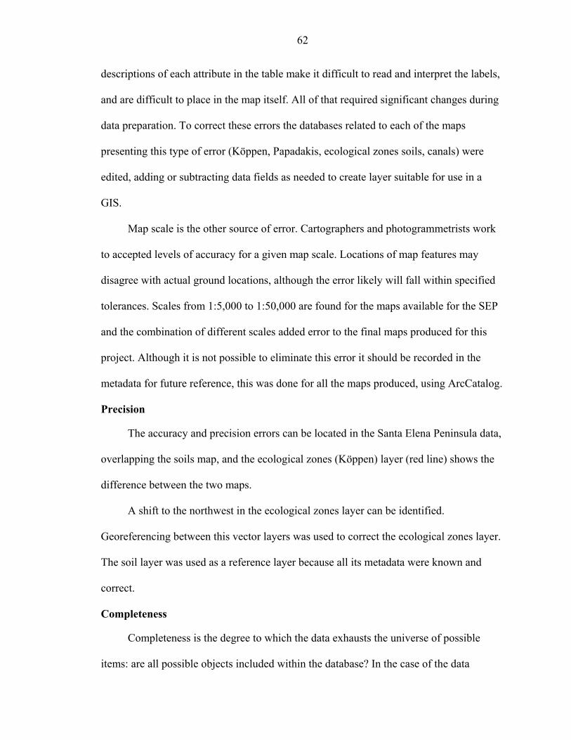
62
descriptions of each attribute in the table make it difficult to read and interpret the labels,
and are difficult to place in the map itself. All of that required significant changes during
data preparation. To correct these errors the databases related to each of the maps
presenting this type of error (Köppen, Papadakis, ecological zones soils, canals) were
edited, adding or subtracting data fields as needed to create layer suitable for use in a
GIS.
Map scale is the other source of error. Cartographers and photogrammetrists work
to accepted levels of accuracy for a given map scale. Locations of map features may
disagree with actual ground locations, although the error likely will fall within specified
tolerances. Scales from 1:5,000 to 1:50,000 are found for the maps available for the SEP
and the combination of different scales added error to the final maps produced for this
project. Although it is not possible to eliminate this error it should be recorded in the
metadata for future reference, this was done for all the maps produced, using ArcCatalog.
Precision
The accuracy and precision errors can be located in the Santa Elena Peninsula data,
overlapping the soils map, and the ecological zones (Köppen) layer (red line) shows the
difference between the two maps.
A shift to the northwest in the ecological zones layer can be identified.
Georeferencing between this vector layers was used to correct the ecological zones layer.
The soil layer was used as a reference layer because all its metadata were known and
correct.
Completeness
Completeness is the degree to which the data exhausts the universe of possible
items: are all possible objects included within the database? In the case of the data
63
available for this project this aspect relates to a “logical consistency”. Basically, it does
not matter if there is a lot of information in a database if that information cannot be used
in an efficient manner.
Figure 4-6. Overlap error
Metadata Errors
Coordinate transformation introduces error, particularly if the projection of the
original document is unknown, or if the source map has poor horizontal control. The
digital maps of the SEP were that the maps were in different projections or did not have
any stated projection; however this is not something difficult to correct. ArcGIS contains
a feature that allows setting the desired coordinate system for a map. The coordinate
system selected for the maps of the SEP was the Universal Transverse Mercator (UTM)
Zone 17 South. It is important to note that bad metadata can be a source of spatial error,

64
especially when trying to overlay different layers. The most accepted standard for
metadata is giving by the Federal Geographic Committee (2000) in the Content Standard
for Digital Spatial Metadata.
Manual Digitizing
Manual digitizing was the method predominantly used to create the digital maps of
the different attributes for the Santa Elena Peninsula (SEP). This digitizing method can
introduce more errors in the final product, especially when done without proper trained
people and without supervision and quality control (Figure 4-5). The digitizing process
was made in ESPOL (Polytechnic School of the Littoral) Guayaquil, Ecuador, in most of
the cases by students and people with little practice in digitizing.
Source Data for the Santa Elena Peninsula
The main problem with the SEP maps is related to many different data sources.
Starting with maps created by various national and international agencies, and digitized
in different manners. Several databases (climatic, agricultural production, water use,
water consumption, etc.) the collected with unknown methods by different institutions. In
addition, there was difficulty to compare this data against other sources because of the
few studies completed in the area of the Peninsula.
Controlling GIS Errors
Data entry procedures should be thoroughly planned, organized and managed to
produce consistent, repeatable results. Nonetheless, a thorough, disciplined quality
review and revision process also is needed to catch and eliminate data entry errors. All
production and quality control procedures should be documented, and all personnel
should be trained in these procedures. Moreover, the work itself should be documented,
including a record of what was done, who did it, when was it done, who checked it, what

65
errors were found, and how they were corrected. GIS data should not be provided without
metadata indicating the source, accuracy and specifics of how the data were entered.
GIS Layers Created or Edited for the Project from the Original Maps
Soils
The new soil map divides all the soils into three groups (silt, sand and clay). The
distribution of these soils within the Peninsula is presented in Figure 4-7. The “merge”
tool in the “Geoprocessing” wizard from Arc View 3.2 was used to simplify this layer.
The original soil map is presented in Figure 4-1.
Figure 4-7. Main soil types layer created for the Santa Elena Peninsula
Ecological Zones
This layer shows the ecological division in the Santa Elena Peninsula. According to
the Köppen method the Peninsula is divided in desert, steppe and savannah.

66
The canals of the TRASVASE irrigation system cross the different ecological
zones. The “clipping” geoprocessing tool available in Arc View 3.2 was used to clip the
canals to the ecological zones (Figure 4-8).
Figure 4-8. Ecological zones
Canals
This figure represents several layers; ecological zones, canals, and the dams in the
area of interest.
The roads, and drainage lines were deleted to create this layer. The layers were also
clipped using the Köppen Ecological Zones. The different materials of the canals where
maintained but join in one canal per ecological zone, this was done to facilitate the
evaporation calculation in the later phase on in the project.

67
Figure 4-9. Canals
Existing Farm Locations
A layer that shows the geographic locations of most of the farms close to the canals
(Figure 4-9) was also created. More detailed maps of the farms locations can be seen in
Appendix A (Figures A-5 to A-8). The farms are grouped in five regions: Santa Elena,
Chongón, Cerecita, and El Azúcar – Rio Verde. This layer shows the total areas of the
farms, however that is not the actual area under agricultural production. As information
about crops produced in each farm becomes available, these layers will be used to create
maps that will show the total area that can be irrigated in each zone according to the
weather parameters and crop water requirements. These concepts will be explained in the
following Chapters.

68
Figure 4-10. Actual farm locations
Weather Stations Location
Known coordinates of each one of the weather stations were used to create a
Microsoft Access database. An “ID and Station Name” fields were added for better
identification of the stations and to be used to link or join this table with others in Arc
View 3.2. With the Access file a shape file was created in Arc View 3.2 so it can be
displayed as a layer in the GIS (Figure 2-5 in Chapter 2).
Weather Data
There are a number of commonly used interpolation techniques described in the
literature, such as simple average, Thiessen polygon, classical polynomial interpolation,
inverse distance, multi quadratic interpolation, optimal interpolation, kriging and others.
In this study the inverse distance interpolation technique was chosen for its simplicity.

69
Researchers have used diverse statistical and geostatistical models to generate
temperature surfaces from point sampling locations. The simplest technique uses the
nearest measurements. Trend surfaces, inverse distance weighted interpolation (IDW),
and thin plate spline, all have been used to interpolate temperature measurements over
global, continental, and broad regional scales. These models, assume the underlying
surface is smooth as it is the topography found in the Santa Elena Peninsula.
Inverse Distance Interpolation. As is obvious for the name of the interpolation
technique, the weighting factor is inversely proportional to the distance. The weights of
this interpolation technique are solely a function of the distance between the point of
interest and the sampling points.
Table 4-1. Comparison of interpolation methods Method Advantages Disadvantages Bi-linear interpolation Simple, conservative Smoothing Polynomial trend surface Designed degree of smoothing Unstable near edges
Inverse square distance weighting
Preserves high frequencies Outliers
Kriging (variogram) Uses variance of data Directional effects Spline interpolation Optimal fit Strong edge effects Laplacian fitting Good fitting, smooth decay at
edges Smoothing
The inverse distance technique does not take advantage of spatial correlation
structure explicitly. However, for climate data these correlation structures tend to be
linear and it is a good guess to assume that the inverse distance weighting would work
fairly well.
The Inverse Distance Weighted interpolation method was used to create the surface
maps (Figure 4-11) with the Geostatistical Analysis Tool from ArcGIS for the weather

70
variables: maximum, minimum and medium temperature, and maximum, minimum and
medium relative humidity. Examples are the surface maps for the month of January
(Figure 4-11).
Inverse Distance Weighted (IDW) interpolation explicitly implements the
assumption that places that are close to one another are more alike than those that are
farther apart. To predict a value for any unmeasured location, IDW will use the measured
values surrounding the prediction location, with values closest to the prediction location
having more influence on the predicted value than those farther away (Johnston, et al.
2001). IDW assumes that each measured point has a local influence that diminishes with
distance, and weights the point closer to the prediction location greater than those farther
away (Johnston, et al. 2001).
( ) (SS ii
io Ζ∑ΖΝ
=
=1λ ) (4-1)
Z(So) value to predict for location So N number of measured points λ weight, these weights will increase with distance Z(Si) observed value at the location Si
The formula to determine the weights is (Johnston, et al., 2001):
∑Ν
=
−−=1i
p
io
p
ioi ddλ (4-2)
11
=∑Ν
=iiλ
As the distance becomes larger, the weight is reduced by a factor of p. The dio value
is the distance between So and Si.
The Inverse Distance Weighted method includes a power (p) parameter. This p
parameter influences the weighting of the measured location’s value on the prediction

71
location’s value; that is, as the distance increases between the measured sample locations
and the prediction location, the weight that the measured point will have on the prediction
will decrease exponentially (Johnston, et al. 2001). The optimal p value is determined by
minimizing the root-mean-square prediction error (RMSPE). The RMSPE is a summary
statistic quantifying the error of the prediction surface (Johnston, et al. 2001).
After one map for each weather variable was created for each month of the year
they were classified into 5 classes because the variation in the data was small. To
reclassify those surface maps the Equal Interval method was used. In the Equal Interval
method the range of possible values is divided into equal-sized intervals. Because there
are usually fewer endpoints at the extremes, the numbers of values are less in the extreme
classes. This method is used in data ranges as percentages (relative humidity or
temperature) (McCoy, and Johnston 2001).
Creation of Evapotranspiration Surface Maps
For this study, the climatic information used to make interpolation is based on
inverse distance weighted method of 5 stations in the Santa Elena Peninsula (SEP). While
interpolation of a value at reach cell in the study area using 5 meteorological stations is
technically easy, some important questions can be raised. Are the stations representative
of the areas around them? How large or small an area do they represent? How does the
spatial feature in question change over space? Is it continuous or discontinuous and
abrupt?

72
Figure 4-11. Surface maps of weather data for January

73
Characterization of climate data for a study area typically relies upon a series of
measurements at discrete locations. Spatial interpolation of these discrete data into a
continuous surface is generally the first step for use with other GIS data layers.
These surface maps layers were used to determine relationships between stations and to
identify the agricultural production zones affected by each of the weather stations.
Weather parameters affect evapotranspiration and as a result they modify irrigation
requirements. Later in this document (Chapter 5, Figures 5-9.1 and 5-9.2) reference
evapotranspiration surface maps are presented to show the monthly variations within the
Santa Elena Peninsula.

CHAPTER 5 WATER AVAILABILITY AND ITS USE IN THE SANTA ELENA PENINSULA
Infrastructure
In the TRASVASE irrigation system the water is used for irrigation and also for
human consumption, and as in any irrigation systems there are losses. To calculate the
total available water for irrigation the amount used for potable water and the losses of the
system have to be calculated.
TRASVASE Santa Elena
Daule – Peripa Dam
This dam (6,000 million cubic meter) works to control floods, regulate water flow,
control salinity levels, and produce hydroelectric power. Because of that its name is
‘Proyecto de Propósito Multiple Jaime Roldós Aguilera’, in English, Multi-purpose
Project ‘Jaime Roldós Aguilera’ (Figures 5-1 and 5-2).
Figure 5-1. Daule-Peripa Dam
74

75
Figure 5-2. Hydroelectric plant, ‘Proyecto de Propósito Multiple Jaime Roldós Aguilera’.
The area directly influenced by this project is 50,000 ha in the Daule Valley.
Indirectly 42,000 ha are projected to be irrigated in the Santa Elena Peninsula. Another
50,000 ha (500 m3/year) are projected to be irrigated from the same Dam in the Manabi
province (CEDEGE 2001).
History of the Project
The Santa Elena Peninsula (SEP) has suffered a water crisis for more than 100
years. Most people agree that deforestation is the main cause, converting what was once
tropical forest to a near desert. To mitigate the drought conditions, and to use this land for
agricultural production the TRASVASE project was built. In 1992 the first hydraulic
structures were put together to start the TRASVASE Daule-Santa Elena.
Following that, the Chongón Dam (Figure 5-3), the Chongón irrigation canal, the
Chongón – Cerecita irrigation canal and the irrigation infrastructure in the Chongón,
Daular and Cerecita irrigation zones were built; total project covering approximately
5,000 ha (CEDEGE 2001).

76
Figure 5-3. Chongón Dam
In order to promote the use of most efficient irrigation techniques, and demonstrate
the agricultural potential in the SEP, pressurized irrigation systems were installed, at
Chongón and Cerecita, consisting of pumping stations, subterranean conveyance pipes,
and portable sprinkler systems.
Figure 5-4. Daule pumping station
At the end of 1995 the construction of the Daule-Chongón canal was completed
assuring constant water supply to the Chongón Dam, the Chongón-Cerecita-Playas canal
and the Daule Pumping Station. Sixty-one kilometers of canals were lined with concrete,

77
and the 6.5 km Cerro Azúl tunnel was finished. It was estimated that this system will
allow the irrigation of 15,000 ha of land (CEDEGE 2001).
In 1998 the first part of the project was finished. In that part the water from the
Chongón Dam was conducted to El Azúcar Dam and from here to the Río Verde
irrigation zone. To accomplish this the following structures were build: the Chongón
Pumping Station, a 3 km pressurized conveyance pipeline, and 40 km of canals lined with
high-density polyethylene. The El Azúcar Dam was refurbished, and the Cola dam in San
Juan (Playas) was built to regulate the water flow.
Table 5-1. Main dams Dams Volume (106 m3) Surface (km2) Water level (m) Max Min Max Min Max Min Chongón 273.6 148.5 25.7 16.9 51 45 El Azúcar 53.8 25 14 8.5 45 42 De Cola 2.44 1.4 0.4 0.5 26.5 24.8
In the last part of this project the Sube y Baja Dam, the Sube y Baja-Javita,
Afaye-Atahualpa, and Villangota and Azúcar-Zapotal canals will be built.
Other important and complementary projects were constructions of two
potabilization plants and wastewater treatment plants in 2000.
Potabilization Plants
The water from the TRASVASE is now also used to supply two water
potabilization plants for two of the larger towns in the Peninsula. One of those is the
Santa Elena plant (Irrigation Zone I), which supplies water for the cities of Santa Elena
and Salinas. The second one provides water to Playas (Irrigation Zone II). The flow water
required by the plants are 1.6 m3/sec and 0.55 m3/sec respectively (CEDEGE 2001).

78
Figure 5-5. Zone II potabilization plant
The construction of sanitary canals in the main cities and towns of the Peninsula is
included in the CEDEGE plans for the SEP. Also planned are controls for prevention of
surface and groundwater contamination.
Transmission Canals
The TRASVASE irrigation system uses canals and pipes to deliver the water to its
users. The seepage loss from the canals constitutes a substantial percentage of the usable
water. Irrigation canals lose water through seepage and evaporation (Chahar 2000). The
seepage loss from canals is governed by hydraulic conductivity of the subsoil, canal
geometry, location of water table relative to the canal, and several other factors (Burton et
al. 1999).
Figure 5-6. Canal
Transmission canals are used in the TRASVASE system to convey water from the
source to a distribution canal. Often the area to be irrigated lies very far from the source,
and hence requires long transmission canals.

79
Figure 5-7. Canal San Rafael, TRASVASE project
Normally, there should be no withdrawal from a transmission canal. In the case of
the TRASVASE this occurs because the secondary (delivery) canals have not been
completed and water from the transmission canals is used to supply irrigation water to the
adjacent land.
The canals of the TRASVASE system are lined with various materials, from
reinforced concrete, to polyethylene, to the original material of the riverbed. To calculate
the seepage losses of each section of the canal we need to know the characteristics of
each of these materials. However, in this study the average number estimated by
CEDEGE (7 %) was used for calculation of seepage losses.
Water Loss from the Canals and Dams to Evaporation
The main causes of loss of stored water are seepage through a leaking basin or dam
wall, and evaporation from the surface. Many methods have been developed for
controlling both, but few are economically attractive (Hudson 1987).
Evaporation from open water can easily reach 7 mm per day in arid or semi-arid
countries. This equals 5 cm per week and 20 cm per month (Brouwer, et al. 1992). The
amount of water lost by evaporation can be considerable, particularly in reservoirs, which
are large and shallow. Therefore, irrigation from shallow lakes and reservoirs should be
started as soon as possible after the rainy season.
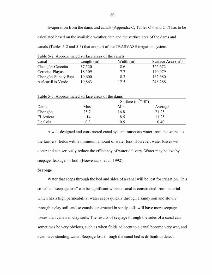
80
Evaporation from the dams and canals (Appendix C, Tables C-6 and C-7) has to be
calculated based on the available weather data and the surface area of the dams and
canals (Tables 5-2 and 5-3) that are part of the TRASVASE irrigation system.
Table 5-2. Approximated surface areas of the canals Canal Length (m) Width (m) Surface Area (m2) Chongón-Cerecita 37,520 8.6 322,672 Cerecita-Playas 18,309 7.7 140,979 Chongón-Sube y Baja 19,600 8.3 162,680 Azúcar-Rio Verde 19,863 12.5 248,288
Table 5-3. Approximated surface areas of the dams Surface (m2*104) Dams Max Min Average Chongón 25.7 16.8 21.25 El Azúcar 14 8.5 11.25 De Cola 0.3 0.5 0.40
A well-designed and constructed canal system transports water from the source to
the farmers’ fields with a minimum amount of water loss. However, water losses will
occur and can seriously reduce the efficiency of water delivery. Water may be lost by
seepage, leakage, or both (Hoevenaars, et al. 1992).
Seepage
Water that seeps through the bed and sides of a canal will be lost for irrigation. This
so-called “seepage loss” can be significant where a canal is constructed from material
which has a high permeability: water seeps quickly through a sandy soil and slowly
through a clay soil, and so canals constructed in sandy soils will have more seepage
losses than canals in clay soils. The results of seepage through the sides of a canal can
sometimes be very obvious, such as when fields adjacent to a canal become very wet, and
even have standing water. Seepage loss through the canal bed is difficult to detect

81
because water goes down and does not appear on the nearby ground surface (Hoevenaars
et al., 1992).
Figure 5-8. Trapezoidal canal
Leakage
Water may also be lost by leakage. This water does not seep, but flows through
larger openings in the canal bed or sides (Hoevenaars, et al. 1992).
• Seepage around structures, leading to severe leakages • Gates which are not tightly sealed • Cracked concrete canal linings, or joints that are not tightly sealed • Torn asphalt or plastic lining
Leakage often starts on a small scale, but the moment that water has found a way
through a canal embankment a hole will develop through which water will leak. If the
leakage is not stopped in time, the tunnel becomes larger and the canal bank may be
washed away at a certain moment. In the case of a lined canal, the canal foundation may
be undermined after some time and the canal will collapse.
Table 5-4. Canal description Canal Length (m) Q (m3/sec) Lining Daule-Chongón (tunnel) 32,723 44 Concrete Chongón-Cerecita 24,494 12 Concrete Cerecita-Playas 31,741 9 Concrete Chongón-Sube y Baja 19,600 9.2 Polyurethane Azúcar-Rio Verde 19,863 5.5 Polyurethane

82
Irrigation Efficiency
The application efficiencies considered for this project were within those defined
by FAO (Table 1-2). The in-field irrigation efficiency values considered were 50 %, 70 %
and 90 %. Using an ample range of efficiencies assures the inclusion of a wide range of
conditions where irrigation is applied to the field.
Irrigation Technology used in the Santa Elena Peninsula
In the period 2000–2001 CEDEGE conducted a survey to the agricultural producers
in the SEP. The results from this survey show the adoption of the latest irrigation
technology by large farmers that have the capital to implement the technology (Tables
5-5 to 5-7).
Table 5-5. Chongón-Daular-Cerecita pressurized system, Zone I (2001) System Area % Drip 19.17 Sprinkler 18.63 Microsprinkler 9.89 Water hose 11.41 Other 2.28 Not using irrigation 38.02
In this zone consisting of 2,780 ha cultivated (Table 5-5) the percentage of farmers
not using any type of irrigation system is highest compared to the other regions. This
corresponds to the area owned by small farmers.
Table 5-6. Chongón-Cerecita-Playas canal, Zone I (2001) System Area % Drip 27.78 Sprinkler 8.89 Microsprinkler 21.11 Water hose 11.11 Not using irrigation 31.11

83
More than half (57 %) of the area in this zone of 3,175 ha under agricultural
production (Table 5-6) is covered by irrigation systems that theoretically will have a field
application efficiency of 70 % of higher.
Table 5-7. El Azúcar-Río Verde canal, Zone II (2001) System Area % Drip 35.4 Sprinkler 7.96 Microsprinkler 3.54 Surface 13.27 Not using irrigation 39.82
The conditions in this area (565 ha cultivated) (Zone II) differ from the previous
two areas (Zone I) because in Zone II the water is scarcer and the irrigation systems used
should be more efficient to overcome that deficit. This can explain the higher use of drip
systems over sprinklers.
Water Consumption
CROPWAT is meant as a practical tool to help agro-meteorologists, agronomists
and irrigation engineers to carry out standard calculations for evapotranspiration and crop
water use studies and more specifically, the design and management of irrigation
schemes. It allows the development of recommendations for improved irrigation
practices, the planning of irrigation schedules under varying water supply conditions, and
the assessment of production under rain fed conditions or deficit irrigation.
Calculations of crop water requirements (CWR) and irrigation requirements are
carried out with inputs of climatic and crop data. Standard crop data are included in the
program and climatic data can be obtained for 144 countries through the CLIMWAT
database. Ecuador is included in this database, however, the data for the Santa Elena
Peninsula is for weather stations that do not represent accurately the weather in this area.

84
The development of irrigation schedules and evaluation of rain fed and irrigation
practices are based on a daily soil-water balance using various options for water supply
and irrigation management conditions. Scheme water supply is calculated according to
the cropping pattern provided for the model.
Reference Evapotranspiration Surface Maps
The first step to calculate CWR is to calculate reference evapotranspiration (ETo).
The process starts by entering historical average weather data for the Santa Elena
Peninsula into CROPWAT (FAO/UN). This is a process that requires careful quality
control since each value has to be entered manually into the system, and errors are easily
made. All weather data (maximum and minimum temperatures and relative humidity,
available wind speed data, and sunshine) for each station was introduced to the
CROPWAT database. Missing parameters like wind speed data (for some months and
stations) and solar radiation were calculated using the same program. Once all the data
was complete, the reference evapotranspiration was calculated using the Penman-
Monteith method.
To create the ETo surface maps, the output from CROPWAT had to be entered to
an ArcMap (ESRI) database to georeference the ETo data set. Inverse distance weighting
(IDW) interpolation method (Chapter 4) was selected to interpolate the reference
evapotranspiration data between the weather stations.
The average monthly surface maps of ETo for the Santa Elena Peninsula (Figures 5-
9.1 and 5-9.2) present the variation in reference evapotranspiration in the months of June
to November considered to be the dry season, and December to April (or May)
considered to be the wet season.

85
These ETo maps plus the precipitation distribution data (Chapter 2) were used later
on in this project (Chapter 6) to determine the crops irrigation requirements in different
irrigation zones.
Crop water requirement (CWR). A specific crop grown in a sunny and hot
climate needs more water per day than the same crop grown in a cloudy and cooler
climate. The highest crop water needs are thus found in areas that are hot, dry, windy and
sunny. The lowest values are found when it is cool, humid and cloudy with little or no
wind (Brouwer & Heibloem 1985).
The crop type impact on the crop water need is important in two ways:
• The crop type influences on the “daily water needs” of a fully-grown crop • Duration of the total growing season depends on the crop.
Data on the duration of the total growing season of the various crops grown in an
area can best be obtained locally. These data may be obtained from, for example, the seed
supplier, the Extension Service, the Irrigation Department or Ministry of Agriculture.
Table 5-8. Crop growing period Crop Total growing period (days) Crop Total growing period (days) Banana 300-365 Onion green 70-95 Bean green 75-90 Onion dry 150-210 Bean dry 95-110 Pepper 120-210 Citrus 240-365 Potato 105-145 Cucumber 105-130 Rice 90-150 Grain/small 150-165. Sorghum 120-130 Maize sweet 80-110 Soybean 135-150 Maize grain 125-180 Squash 95-120 Melon 120-160 Sunflower 125-130 Tomato 135-180
* Modified from Irrigation Water Management, Training manual no. 3, FAO

86
Figure 5-9.1. Average reference evapotranspiration for the SEP I

87
Figure 5-9.2. Average reference evapotranspiration for the SEP II

88
When the plants are very small, the evaporation from the soil will be more
important than the transpiration. When the plants are fully-grown, the transpiration is a
larger component of total water loss than the evaporation. At planting and during the
initial stage, the evaporation is more important than the transpiration and the
evapotranspiration or crop water need, during the initial stage, is estimated at 50 percent
of the crop water need during the mid - season stage, when the crop is fully developed.
During the so-called crop development stage, the crop water need gradually increases
from 50 percent of the maximum crop water need. The maximum crop water need is
reached at the end of the crop development stage, which is the beginning of the mid-
season stage.
To estimate the water use of the cultivated area in the Santa Elena Peninsula (SEP)
some concepts have to be defined first to understand the calculations made to obtain the
crop water requirement (CWR) values. To calculate these values the CROPWAT
software from FAO was used.
Crop coefficients. While reference crop evapotranspiration (ETo) accounts for
variations in weather and offers a measure of the evaporative demand of the atmosphere,
crop coefficients account for the difference between the crop evapotranspiration (ETc)
and ETo.
Because evapotranspiration (ET) is the sum of evaporation (E) from soil and plant
surfaces and transpiration (T), which is vaporization that occurs inside of the plant leaves,
it is often easier to consider them together as ET (Stroosnijder 1987). When not limited
by water availability, both transpiration and evaporation are limited by the availability of

89
energy to vaporize water. Therefore, solar radiation interception by the foliage and soil
has a big effect on the ET rate (Allen et al. 1998).
Table 5-9. Crop coefficients
Crop Kc ini Kc mid Kc end Maximum Crop Height
Small Vegetables 0.7 1.05 0.95 Garlic 1.00 0.70 0.3 Onions dry 1.05 0.75 0.4 green 1.00 1.00 0.3 Vegetables - Solanum Family (Solanaceae)
0.6 1.15 0.80
Sweet Peppers (bell) 1.05 0.90 0.7 Tomato 1.15 0.70-0.90 0.6
Vegetables - Cucumber Family (Cucurbitaceae)
0.5 1.00 0.80
Cantaloupe 0.5 0.85 0.60 0.3 Cucumber Fresh Market 0.6 1.00 0.75 0.3 Pumpkin, Winter Squash 1.00 0.80 0.4 Watermelon 0.4 1.00 0.75 0.4 Roots and Tubers 0.5 1.10 0.95 Potato 1.15 0.75 0.6 Legumes (Leguminosae) 0.4 1.15 0.55 Beans, green 0.5 1.05 0.90 0.4 Perennial Vegetables (with winter dormancy and initially bare or mulched soil)
0.5 1.00 0.80
Asparagus 0.5 0.95 0.30 0.2-0.8 Cereals 0.3 1.15 0.4 Maize, Field (grain) (field corn) 1.20 0.60-0.35 2
Maize, Sweet (sweet corn) 1.15 1.05 1.5 Rice 1.05 1.20 0.90-0.60 1 Forages Grazing Pasture Extensive Grazing 0.30 0.75 0.75 0.10 Tropical Fruits and Trees Banana 1st year 0.50 1.10 1.00 3 2nd year 1.00 1.20 1.10 4 Cacao 1.00 1.05 1.05 3 Coffee bare ground cover 0.90 0.95 0.95 2-3

90
with weeds 1.05 1.10 1.10 2-3 Pineapple bare soil 0.50 0.30 0.30 0.6-1.2 with grass cover 0.50 0.50 0.50 0.6-1.2 *continuation Table 5-9
Crop Kc ini Kc mid Kc end Maximum Crop Height
Grapes and Berries Grapes Table or Raisin 0.30 0.85 0.45 2 Wine 0.30 0.70 0.45 1.5-2 Fruit Trees Avocado, no ground cover 0.60 0.85 0.75 3 Citrus, no ground cover 70% canopy 0.70 0.65 0.70 4 50% canopy 0.65 0.60 0.65 3 20% canopy 0.50 0.45 0.55 2 Citrus, with active ground cover or weeds
70% canopy 0.75 0.70 0.75 4 50% canopy 0.80 0.80 0.80 3 20% canopy 0.85 0.85 0.85 2 Based on Tabulated Kc (Table 12), Paper # 56 FAO (Allen et al. 1998).
As a crop canopy develops, the ratio of T to E increases until most of the ET comes
from T and E is a minor component. This occurs because the light interception by the
foliage increases until most light is intercepted before it reaches the soil.
Commercial irrigation schedules typically begin their computation with published
regional crop coefficients. These coefficients, when multiplied by reference crop
evapotranspiration, are used to calculate crop evapotranspiration. These regional crop
coefficients are based on a certain reference crop, soil type and irrigation management
practice. In conventional agriculture irrigation scheduling, crop coefficients can be
modified as needed during the growing season, because there is constant feedback based
on field observations of crop and soil conditions.

91
Agricultural Production in the Santa Elena Peninsula
Ecuador, with its climatic conditions, could be completely self-sufficient in food
production and even produced for export. However, today most of the subtropical fruits
(deciduous, grapes, citrus, etc.) are imported from Chile or California. Many areas of the
country are considered very dry (less than 500 mm of water a year) and are therefore not
included in the agricultural production cycle. Ecuador has several state water projects that
were built many years ago, however, most are not in operation.
According to CEDEGE (2001) the TRASVASE Daule-Santa Elena Project is the
largest and most modern irrigation project in Ecuador. Until 1994 there was no source of
water for irrigation in the SEP and the few wells sunk had a low capacity and were
mostly saline. On completion of the first part of the project, about 15,000 hectares were
brought into the production potential and today, with completion of the second part, the
entire 40,000 hectares are suited for irrigated crops. However, in 1995, a total of about
2,000 hectares were under cultivation and the farmers of the peninsula (large and small)
did not in fact know where to invest and how to utilize the potential of the zone.
The agricultural production in the Santa Elena Peninsula has been limited to few
crops. Even those few crops were planted without any suitability study. Crops like
mangos were planted in zones with heavy soils, and pronounced slopes often without a
good drainage. In other farms, cocoa trees were planted in flat and low land, and then “El
Niño” came in 1997, flooding most of the area and killing the plantations. Stories like
these can be found throughout the Peninsula. In addition, poor market study and lack of
governmental policies to control the planted area affected the price in the international
markets, because of an excessive offer of the product (Mango, Onion, Passion Fruit).

92
The large farms in the Santa Elena Peninsula are mainly focused towards export
products, and only the excess or products that do not meet the international standards are
left for the local (internal) market. The main market for onion is Colombia and Peru,
while passion fruit is transformed into concentrate and exported to the U.S. and European
markets. Tomato is used by the local industry, and pineapple is exported as fresh and
canned fruit. Bananas were first planted in the SEP because it was thought that the dry
conditions in the area would help to control the fungus Mycosphaerella fijinsis or
Sigatoka. But even though the Santa Elena Peninsula is considered a dry area because of
the soil characteristics and the reduced rainfall, it has a high relative humidity (average >
80 %), and relative humidity promotes the development of fungus. As a result, the banana
planted area is being reduced. Plantain is far more resistant and resilient than banana to
Sigatoka. Yields from 5 crops (Figure 5-10) were obtained from CEDEGE in 2001.
Production in the SEP
0 10 20 30 40 50 60 70 80
Banana
Pineapple
Tomato
Passion F.
Onion
TON/Ha
Figure 5-10. Agricultural Production in the Santa Elena Peninsula
In 2000 CEDEGE conducted a survey to the farmers using water from the
TRASVASE project in the areas adjacent to the canals, dams, and covered by the
pressurized irrigation zones, the results about land use are presented in Table 5-10. The

93
data for 200o is the actual area under production, and the data for 2001 are the estimated
increase in area.
Table 5-10. Crops planted and projected increase in the Santa Elena Peninsula Crops planted and projected in the Santa Elena Peninsula
Zone I Zone II Chongón-Daular Chongón-Playas El Azúcar-Rio Verde
Crops 2000 2001 2000 2001 2000 2001 Asparagus 20 Avocado 5 22 40 Banana 60 Beans 4 8 Black Pepper 1 Cassava 6 Plum 11 Citrus 74 2 26 Cocoa 241 127 492 60 2 54 Corn 364 155 244 168 263 Cotton 16 Cucumber 14 1 Flowers 21 Grape 8 6 7 Grass 198 22 5 20 8 Green pepper 11 19 19 Guava 24 201 100 Guanabana 28 40 Hot pepper 24 4 Lime 451 20 178 Mango 852 89 1343 171 Melon 51 15 12 Onion 75 213 70 132 38 Palm 4 Papaya 10 13 16 50 Pineapple 45 Pitahaya 10 Plantain 184 25 388 6 Rice 44 8 9 Soya 8 Teak 105 100 Tobacco 10 Tomato 5 15 Watermelon 23 14 12 14 Wheat 11 Other 19 37 14 17

CHAPTER 6 METHODOLOGY
Water available from the TRASVASE project is mainly utilized for irrigation. One
of the objectives of this project was to determine the total area that can be irrigated using
this water. The extent of irrigated land was determined by calculating the crop water
requirement of crops grown in the area using CROPWAT, a model developed by
FAO/UN. This model requires monthly averages of weather parameters that were
calculated from the available data from the Santa Elena Peninsula.
CROPWAT was reviewed in Chapter 5. To calculate water requirement (CWR) for
each crop the required data are: evapotranspiration, crop coefficients, crop area, and
planting dates.
Weather data for the CROPWAT were based on the monthly averages calculated
from the data provided by CEDEGE. The variables (Figure C-1) entered were average
temperature (oC), average relative humidity (RH), average wind speed (m/s or km/day),
and daily average sunshine (hr/day). Built into the CROPWAT are the processes to
calculate ‘missing’ weather parameters as explained in “Estimating missing climatic
data” section in Chapter 3. This technique was used to calculate the solar radiation
(MJ/m2/d).
Evapotranspiration
CROPWAT calculates the evapotranspiration (ETo) values for each month for
every weather station in the Santa Elena Peninsula based on the provided weather data.
These evapotranspiration values (ETo) are presented in Appendix C (Tables C-1 to C-5).
94

95
A revised method for estimating reference crop evapotranspiration, adopting the
approach of Penman-Monteith as recommended by the FAO Expert Consultation in
Rome is used in this model. Further details on the methodology are provided in the
Irrigation and Drainage Paper No 56: "Crop Evapotranspiration" (Allen, et al. 1998).
Open Water Evaporation
In Tables 5-1 and 5-3 the approximated surface areas based on available
dimensions for all canals and dams in the TRASVASE project are presented. Average
evapotranspiration values calculated using CROPWAT for the same zones used to
calculate crop water requirement (CWR), were used to estimate the evaporation from the
canals and dams. The open water evaporation per month has been calculated with the
following equation developed by Smith (1996):
E = kw * ETo (6-1)
where:
E: Open water evaporation ETo: Penman Monteith reference evapotranspiration kw: correction factor for open water evaporation
Reference evapotranspiration values came from CROPWAT, and the correction
factor used for open water evapotranspiration is 1.3, based on Smith (1996) and
recommended by FAO as a global average for open water evaporation when local data is
not available. The value of 1.3, therefore, is an arbitrary value valid only under average
conditions.
The monthly evaporation values for each canal, and dam are presented in Appendix
E (Tables E-1 and E-2 respectively). Since evaporation is directly proportional to the
evapotranspiration data these values are the highest in the month of April followed by

96
November for all the weather stations. The monthly changes in evaporation in cubic
meters from the different canals are presented here (Figure 6-1).
Evaporation from canals
400
600
800
1000
1200
Janu
ary
Februa
ryMarc
hApri
lMay
June Ju
ly
Augus
t
Septem
ber
Octobe
r
Novem
ber
Decem
ber
Wat
er (c
ubic
met
ers)
Chongon-Cerecita Cerecita-Playas Chongon-Sube y Baja Azucar-Rio Verde
Figure 6-1. Evaporation from canals of the TRASVASE system
Crop Water Requirement
Once crop water requirements (CWR) were calculated, for the known location of
the weather stations, the average values were calculated for the areas surrounding the
specific canals and dams.
These areas were: Chongón-Cerecita canal influenced by the Chongón and San
Isidro weather stations, Cerecita-Playas canal under the influence of the San Isidro and
Playas stations, and De Cola dam influenced by Playas weather station. Chongón dam
under the Chongón station, and Chongón-Sube y Baja canal is influenced by Chongón
and El Azúcar weather stations, El Azúcar dam is under the influence of El Azúcar
weather station as it is the El Azúcar-Rio Verde canal.

97
Table 6-1. Chongón-San Isidro, Zone I, crop water requirements (CWR) Crop Water Requirements (CWR) Chongón-San Isidro, Zone I (mm)
Jun Jul 63.2 73.9
Plantain 50.8
Month Jan Feb Mar Apr May Aug Sep Oct Nov DecAvocado 84.2 78.6 74.9 70.7 75.2 72.9 Asparagus 63.4 79.5 90.9 61.1
50.7 49.5 57.2 100.793.0 97.3 97.1 15.7 Citrus 71.2 71.1 69.4 66.5 84.3 60.3 59.2 59.7 62.1 64.8 66.7 58.1Grapes-t 40.6 40.6 39.6 38.0 49.7 55.3 74.0 77.6 81.2 84.8 82.2 45.7Mango 91.1 91.2 89.2 88.8 122.095.4 97.3 100.5103.7 104.3 99.5 78.7Onion 74.1 77.9 92.9 92.2 38.7 Pineapple 49.1 40.3 29.7 28.5 19.1 Potato 57.5 89.2 114.0100.524.9 Melon 55.4 89.5 105.0 91.5 Watermelon 54.9 68.6 100.0 89.0 S-Pepper 74.7 85.2 105.0 102.0 B-Pepper 62.6 77.0 102.498.5 74.1 77.9 92.9 91.0 *t = table, S= sweet, B=black
Table 6-2. San Isidro-Playas, Zone I, crop water requirements (CWR) Crop Water Requirements (CWR) San Isidro-Playas, Zone I (mm)
Month Jan Feb Mar Apr May Jun Jul Aug Sep Oct Nov DecAvocado 77.7 91.5 104.7 97.3 78.1 85.1 89.4 86.0 Asparagus 75.5 93.8 107.2 72.2 Plantain 62.5 62.7 61.5 70.8 123.1 111.8 115.7 114.6 18.5 Citrus 87.5 87.9 86.2 82.3 103.1 72.5 70.3 70.4 58.8 76.6 79.2 69.2Grapes-t 50.0 50.2 49.2 47.0 60.7 66.5 88.0 91.6 95.7 100.2 97.6 54.4Mango 112.1 112.8 110.8 109.9 149.1 114.9 115.7 118.6 123.5 123.3 119.3 93.8Onion 90.6 93.7 110.4 108.8 45.6 Pineapple 60.3 49.8 36.9 35.3 21.2 Potato 70.7 110.2 141.6 124.4 30.6 Melon 65.4 105.5 124.1 108.6 Watermelon 64.8 100.9 118.2 105.7 S-Pepper 88.2 100.4 124.1 121.1 B-Pepper 76.9 95.3 127.2 121.9 90.6 93.7 110.4 107.5
Monthly crop water requirements (mm) were calculated for 13 crops: avocado,
asparagus, citrus, grapes, mango, melon, onion, pineapple, plantain, potato, black pepper,
sweet pepper, and watermelon. The calculations were done for three areas: Chongón-San
Isidro, San Isidro-Playas, and Chongón-El Azúcar.

98
Table 6-3. Chongón-El Azúcar, Zone II, crop water requirements (CWR) Crop Water Requirements (CWR) Chongón-El Azúcar, Zone II (mm)
Month Jan Feb Mar Apr May Jun Jul Aug Sep Oct Nov DecAvocado 64.0 75.7 87.4 81.9 77.8 72.6 76.0 72.6 Asparagus 64.2 79.3 89.6 61.5 Plantain 51.5 51.9 51.4 59.7 104.6 95.4 98.4 96.7 15.5 Citrus 72.1 72.7 72.0 69.3 87.6 61.9 59.8 59.4 61.2 63.6 65.6 57.7Grapes-t 41.2 41.5 41.1 39.6 51.6 56.7 74.8 77.3 80.1 83.1 81.0 45.2Mango 92.7 93.5 92.5 92.5 126.7 98.0 98.4 100.2 102.1 102.4 97.9 78.1Onion 77.0 79.9 93.9 91.8 38.2 Pineapple 49.7 41.2 30.8 29.7 9.6 Potato 58.3 91.5 118.8 104.8 25.9 Melon 55.2 88.2 103.0 90.1 Watermelon 54.7 67.3 98.1 87.7 S-Pepper 74.5 83.9 103.0 102.1 B-Pepper 63.4 78.9 106.2 102.7 77.0 79.9 93.9 90.7
CROPWAT was used to calculate reference evapotranspiration (ETo) for each
weather station (Appendix C); crop information was used to calculate actual crop
evapotranspiration for 13 crops under consideration (Appendix E). This crop data
consists of crop coefficient, date when the crop is planted on the field, and percentage of
the total area occupied by the crop. In this case the program was run for each crop and the
area covered for each crop was considered 100 % of the total area. The crop coefficients
came from those already into the CROPWAT database (CLIMWAT 1994) and for those
not in CLIMWAT the crop coefficients where entered from the data in Table 5-12 also
obtained from FAO/UN. The planting dates for each crop were entered following the
recommendations of ESPOL (Polytechnic School of the Littoral, Guayaquil) (Appendix
D) that takes into consideration seasonal effects and in some other cases market
advantages.

99
Crop Irrigation Requirement
Crop irrigation requirement (CIR) is the total water needed for the crop (CWR)
multiplied by an in-field irrigation application efficiency factor. These irrigation
application efficiency factors were taken from the estimates given by FAO (Table 1-2).
The values used for application efficiency in this study are 50 %, 70 % and 90 %
efficiency. Fifty percent application efficiency represents a well-managed surface
irrigation system or poor maintained and administered sprinklers or micro-irrigation
systems. Seventy percent efficiency could be well maintained and managed sprinklers
systems, or poorly managed micro-irrigation systems. Ninety percent efficiency
represents well-managed and maintained micro-irrigation systems.
Various scenarios were analyzed. Calculations of water requirement for land
planted with crops with high irrigation requirements, low irrigation requirements, and a
mixture of high and low irrigation requirement were made to be used in this project, for
each of the efficiencies described above. These data are presented in Appendix F.
Scenarios
To facilitate the calculation of the total water resource for certain types of
production, and to follow Köppen ecological classification and the climatic parameters
associated with each classification (Chapter 2, Climatic Classification Section), the
TRASVASE system was divided in two main zones (Figure 6-2).
Zone I: Chongón-Cerecita, Cerecita-Playas canals, Daular, Cerecita, and Chongón
irrigation zones, Zone I (Playas, Table 5-2) potabilization plant, and the Chongón, San
Isidro, and Playas weather stations. Zone II: Chongón-Sube y Baja, El Azúcar-Rio Verde
canals, El Azúcar and Chongón dams, Zone II (Santa Elena, Table 5-2) potabilization
plant, and Chongón, and El Azúcar weather stations.

100
A map using ArcMap (ESRI) was created to show the two zones, the yellow areas
represent Zone I, and the green areas represent Zone II (Figure 6-2).
Figure 6-2. Irrigation zones in the Santa Elena Peninsula
Nine scenarios were created to calculate the water available for agricultural
production and the area that can be irrigated with that amount of water. The water inputs
into the system were: water from the dams. The water available for irrigation was
calculated by subtracting seepage losses of the system; water used in the water treatment
plants, and evaporation losses from the canals and dams. The only changing parameters
among the scenarios are crop types and the types of irrigation system that affects in-field
efficiency.
Scenario A, a surface irrigation system with an in-field efficiency of 50 %, and all
the 13 crops with available crop water requirement (CWR) data. These 13 crops are:

101
avocado, asparagus, citrus, grapes, mango, melon, onion, pineapple, plantain, potato,
black pepper, sweet pepper, and watermelon; evenly distributed to cover 100 % of the
area, the same procedure was repeater for scenarios B and C.
Scenario B, a sprinkler irrigation system with an in-field efficiency of 70 %, all the
13 crops with available crop water requirement (CWR) data.
Scenario C, a micro-irrigation system with an in-field efficiency of 90 %, all the
13 crops with available crop water requirement (CWR) data.
Scenarios A, B, and C, all assume 100 % replacement of evapotranspiration in the
month (August) of the highest evapotranspirational demand.
Scenario AA, surface irrigation system with an in-field efficiency of 50 %,
avocado, plantain, citrus, grapes, and mango, considered as high water requirement crops
(CWR). These crops are in this group for their monthly evapotranspirational demand and
also because the extended growth period they have. The same crops are used in scenarios
BA, and CA.
Scenario BA, sprinkler irrigation system with an in-field efficiency of 70 %, and
high water requirement crops (CWR).
Scenario CA, micro-irrigation system with an in-field efficiency of 90 %, and high
water requirement crops (CWR).
Scenarios AA, BA, and CA, all assume 100 % replacement of evapotranspiration in
the month (August) with the highest evapotranspirational demand.
Scenario AB, surface irrigation system with an in-field efficiency of 50 %,
asparagus, melon, onion, potato, black pepper, sweet pepper, and watermelon are
considered low water requirement crops (CWR), these crops have a short growth period

102
and their evaporatranspirational demand is relatively small compared to those crops
considered as high irrigation requirement crops. These low water requirement crops are
used in scenarios BB, and CB.
Scenario BB, sprinkler irrigation system with an in-field efficiency of 70 %, and
low water requirement crops (CWR).
Scenario CB, micro-irrigation system with an in-field efficiency of 90 %, and low
water requirement crops (CWR).
Scenarios AB, BB, and CB, also assume 100 % replacement of evapotranspiration
in the month (August), the month with the highest water requirement.
To calculate the output of the different scenarios quickly a spreadsheet program
was developed using Excel®. The program is based on the crop water requirement data
produced by CROPWAT. Inputs required by the program are crop area (percentage of
total area), and in-field irrigation efficiency (i.e. 50 % surface irrigation, 70 % sprinklers,
and 90 % micro-irrigation). The output is given in millimeters (mm) of water per month
for each one of the crops selected. To select a given crop an area (percentage have to be
entered in the spreadsheet, to deselect a crop a zero (0) has to be entered for that specific
crop.

CHAPTER 7 RESULTS AND DISCUSSION
The results for this project are based on the multiple scenarios described in
‘Methodology’ (Chapter 6). In this Chapter, the outcome of each scenario will be
discussed and compared to the other scenarios.
As presented in Chapter 2, there are two months (April and August) with the
highest evapotranspiration values. However, April is at the end of the rainy season and
will still receive some rainfall (Figure B-1) and only supplemental irrigation may be
required at this time. In addition, heavy soil texture (clays) (Figure 4-5) results in some
water retention that can be used by the crops at the beginning of the dry season lowering
irrigation requirement.
The month of August is in the dry season with at least two dry months before it.
During this time all the available water likely comes from irrigation. As a result, August
is clearly the month of the highest irrigation demand and is used in this study to
determine the maximum area that can be irrigated with the water from the dams of the
TRASVASE system.
A complete explanation of how these results were obtained is presented for the
following scenario (Scenario A). The total irrigated area consists of Zone I and II. For
Zone II (Table 7-1) the water comes from the El Azúcar-Rio Verde and Chongón-Sube y
Baja canals, and El Azúcar dam (Table 7-1). There are 13 crops (avocado, asparagus,
citrus, grapes, mango, melon, onion, pineapple, plantain, potato, black pepper, sweet
pepper, and watermelon) planted in the zone. These crops represent a mixture of crop
103

104
irrigation requirement (CIR) from high to low. However, not all the crops are growing
during the month of August according to the recommendations by ESPOL and CEDEGE.
In-field irrigation efficiency (application efficiency) is assumed to be 50 % with 100 %
evapotranspiration replacement. Fifty percent efficiency indicates surface irrigation or
poor management of pressurized irrigation systems. Zero (0) precipitation in the area is
assumed.
Table 7-1. Scenario A, Zone II Water Lost Evaporation from m3 Canals: Chongón - Sube y Baja 502 El Azúcar - Rio Verde 690 Dams: El Azúcar 41,828 Potabilization Zone II 1,073,600 Seepage losses from canals: 7% 210,000 TOTAL water lost 1,326,620 Available Water CIR/zone m3 m3/ha Irrigation Zones El Azúcar 2,000,000 1,080Canals Chongón - Sube y Baja 1,000,000 1,080 El Azúcar - Rio Verde 2,000,000 1,080
TOTAL available water 5,000,000 Area that can be irrigated at 50% application efficiency is 3,401ha.
The amount of water that is available for irrigation is calculated as a difference
between total water available from the dams and various losses in the system. The losses
in Zone II include: potabilization plant, seepage losses from the canals, and evaporation
from the canals and the dams. The difference between available water and losses is
divided by the monthly crop irrigation requirement (CIR) value (Table F-3) that was
multiplied by the application efficiency factor (0.5 for 50 % efficiency, in this case). The
parameters in each scenario can be defined as follows: evaporation (canals and/or dams)
refers to the potential evaporation from an open water body (Appendix C, Tables C-6 and

105
C-7) expressed in cubic meters (m3). Potabilization is the water used in the water
treatment plants (Zones I and II, defined in Chapter 6) estimating 12 working hours per
day for 30 days. Seepage losses (Chapter 5) are calculated for the canals in each zone
using 7 % (a value provided by CEDEGE2). Available water is the total water available
from the dams in cubic meters (m3) minus losses in canals or conveyance losses in
pressurized irrigation systems. Crop irrigation requirement or CIR (Appendix F. Tables
F-1 to F-3) is expressed in cubic meters (m3). The total area that can be irrigated is
calculated in hectares (1 ha = 10,000 m2) from the water available from the system and
the CIR.
Table 7-2. Scenario A, Zone I Water Lost Evaporation from m3 Canals: Chongón - Cerecita 1,064 Cerecita-Playas 528 Potabilization Zone I 712,800 Seepage losses from canals: 7% 350,000 TOTAL water lost 1,064,392 Available Water CIR/zone m3 m3/ha Irrigation Zones Chongón 648,000 1,080 Daular I 617,040 1,080 Daular II 816,480 1,080 Cerecita I 479,520 1,080 Cerecita II 1,089,360 1,080Canals Chongón - Cerecita 2,500,000 1,080 Cerecita-Playas 2,500,000 1,280 TOTAL available water 8,044,872
Area that can be irrigated at 50% application efficiency is 6,662ha.
The same procedure was conducted for Scenario A Zone I (Table 7-2). The
differences are in the water sources, Chongón-Cerecita, Cerecita playas canals, and
2 CEDEGE, Comision de Estudios para el Desarrollo de la Cuenca del Rio Guayas, in English, Commission for the Development of the Guayas River Basin.

106
conveyance pipe systems for Chongón, Daular I and II, Cerecita I and II irrigation. The
losses are seepage from the canals, evaporation from canals, and the water used in the
Zone II potabilization plant.
In Scenario A, the areas calculated for Zones I and II were added to calculate the
‘total’ area that could be irrigated under the given conditions for this scenario (Chapter 6,
Scenario A). The total area becomes 10,063 ha for the month of August that is the month
with the highest evapotranspiration. If some water stress would be permitted, for example
80 % or 90 % replacement, more area could be irrigated. Depending on the planting
schedule, more area might be irrigated in other months than August since the calculations
were performed for the month with the highest crop irrigation requirement (CIR).
Table 7-3. Total area that can be irrigated under different scenarios Area that can be irrigated by scenario (ha)
Scenario Zone I Zone II Total Area
Efficiency (%)
Crop water requirement
Water replacement (%)
A 6,662 3,401 10,063 50 Mix: high and low 100 B 7,683 3,950 11,633 70 Mix: high and low 100 C 9,049 4,650 13,699 90 Mix: high and low 100
AA 4,961 2,739 7,700 50 High 100 BA 5,847 3,161 9,008 70 High 100 CA 6,912 3,733 10,645 90 High 100 AB 7,382 3,988 11,370 50 Low 100 BB 8,519 4,603 13,122 70 Low 100 CB 10,064 5,442 15,506 90 Low 100
All the scenarios follow the same procedures. The only differences are the crops
used to calculate crop irrigation requirement and the levels of in-field irrigation
efficiency.
The results from the other scenarios are summarized in Table 7-3. The parameters
to be considered in this discussion are the irrigation efficiency, and the water requirement

107
(Tables 6-1 to 6-3) by crops in each scenario. The crop irrigation requirements (CIR)
calculated for the scenarios are presented in Appendix F.
Scenario B has the same crops as Scenario A. The difference is the in-field
efficiency of the irrigation system is increased from 50 % to 70 %. Under these
conditions the total irrigable area increases by almost 1,600 ha to 11,633 ha. This is a
good indicator how important are the changes in irrigation technology and irrigation
management skills to improve the application efficiency of the irrigation systems in the
Santa Elena Peninsula.
Scenario C has the same 13 crops (Appendix E) as scenarios A and B, but is
assuming a high application efficiency (90 %) of the irrigation system. This positively
affects the area that can be irrigated for Zone I as well as for Zone II reaching a
maximum of 13,699 ha.
These three scenarios are calculated for August, the month with the highest crop
irrigation requirement. This means that for other months with a smaller CIR there is some
excess water in the system and this should be considered when planning the planting
chronogram for the entire season (year).More area can be irrigated during months with
less total crop irrigation requirement, and annual crops with short growing season can be
planted at that time to take advantage of this excess water. For perennial crops the area is
constant. In some cases, or in the first few years of the plantation, intercropping systems
can be used in some fields. That will allow more agricultural production within the same
area and better use of available water.
Scenario AA uses high irrigation requirement crops (CIR) avocado, plantain,
citrus, grapes, and mango; a low in-field irrigation efficiency of 50 % that can be

108
considered as surface irrigation. According to the data obtained by ESPOL3 (Tables 5-7
to 5-9) up to 13 % of the farmers use an irrigation system with this efficiency (50 %) in
the El Azúcar-Rio Verde area (Zone II). Almost 30 % less area can be irrigated under this
scenario as compared to Scenario A. This area reduction may be required, if the majority
of the area within the TRASVASE irrigation system is dedicated to the crops with high
water requirement, under low efficiency irrigation.
Scenario BA is a scenario with the same crops as Scenario AA but with an
efficiency increased to 70 %. That gives almost a 20 % increase in total area (9,008 ha)
compared to the previous scenario. A mixture of high efficiency (micro-irrigation) and
low efficiency (surface) irrigation methods can create a 70 % overall efficiency. The
entire area irrigated using well design and managed sprinkler systems would also result in
similar application efficiency.
Scenario CA considers the following combination of parameters: 90 % in-field
efficiency, 100 % replacement of water lost, and high CIR crops. The total area that can
be irrigated increases to 10,645 ha, similar to that achieved under Scenario A, using all 13
crops instead of just 5 with high irrigation requirement (CIR) as in this scenario.
However, scenario A assumed lower application efficiency.
Scenario AB is a scenario that uses crops with low water requirements (asparagus,
melon, onion, potato, black pepper, sweet pepper, and watermelon), and irrigation
efficiency of 50 %. Even using a low efficiency or poor managed irrigation system, the
low water consumption by the crops compensates the high losses increasing the total area
that can be irrigated under this scenario to 11,370 ha (Table 7-3). This area is greater that
3 ESPOL, Escuela Superior Politecnica del Litoral, in English, Littoral Polytechnic School.
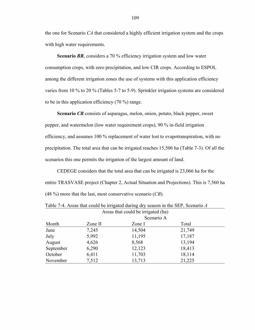
109
the one for Scenario CA that considered a highly efficient irrigation system and the crops
with high water requirements.
Scenario BB, considers a 70 % efficiency irrigation system and low water
consumption crops, with zero precipitation, and low CIR crops. According to ESPOL
among the different irrigation zones the use of systems with this application efficiency
varies from 10 % to 20 % (Tables 5-7 to 5-9). Sprinkler irrigation systems are considered
to be in this application efficiency (70 %) range.
Scenario CB consists of asparagus, melon, onion, potato, black pepper, sweet
pepper, and watermelon (low water requirement crops), 90 % in-field irrigation
efficiency, and assumes 100 % replacement of water lost to evapotranspiration, with no
precipitation. The total area that can be irrigated reaches 15,506 ha (Table 7-3). Of all the
scenarios this one permits the irrigation of the largest amount of land.
CEDEGE considers that the total area that can be irrigated is 23,066 ha for the
entire TRASVASE project (Chapter 2, Actual Situation and Projections). This is 7,560 ha
(48 %) more that the last, most conservative scenario (CB).
Table 7-4. Areas that could be irrigated during dry season in the SEP, Scenario A Areas that could be irrigated (ha)
Scenario A Month Zone II Zone I Total June 7,245 14,504 21,749 July 5,992 11,195 17,187 August 4,626 8,568 13,194 September 6,290 12,123 18,413 October 6,411 11,703 18,114 November 7,512 13,713 21,225

110
The total areas that could be irrigated during the dry season (June, July, August,
September, October, November) in the Santa Elena Peninsula and compared to the values
to the values given by CEDEGE and the farmers (Chapter 2) are given in Figure 7-4.
June and November are close to the numbers given by CEDEGE (Table 7-5).
However, especially for August the crops will be subject of stress if the same area
(23,066 ha) is maintained in this month.
In Figure 7-1 the buffers created at each side from the canals represent the areas
that could be irrigated under different circumstances.
Figure 7-1. Buffers from the canals in the Santa Elena Peninsula

111
Apart of water limitation there are other limiting factors such as the cost of
conveying water far away from the main canals and also the higher losses associated with
this process.
The areas that theoretically could be irrigated assuming different buffers at each
side of the canals are presented in Table 7-5, comparing those values to three of the
scenarios for this project. The three selected scenarios represent 70 % application
efficiency and three crop selections (Table 7-6).
Table 7-5 Areas covered by different buffers of the canals in the SEP Buffer Size (Meters at each side of the canal) Area (ha) Areas by scenario (ha) 250 7,600 B- 11,633 500 15,200 BA- 9,008 1,000 30,400 BC- 13,122
Comparing the values given by CEDEGE, the associations of farmers, and the
values obtained in this project (Table 7-6), it can be noticed that the values calculated
(Chapter 7) in this project are closer to those given by the farmers association, and are
approximately 50% of the area that can be irrigated according to CEDEGE estimates.
Table 7-6. Comparison of areas that could be irrigated according different sources Comparison of areas that could be irrigated according different sources
(Chapter 7) 70% application efficiency (Chapter 2) Scenarios (ha) B BA BC CEDEGE Farmers Assoc. Actual Mix of crops High irrigation Low irrigationPredicted (ha) Predicted (ha) Production (ha) Requirement Requirement 23,000 16,000-17,000 6,900 11,633 9,008 13,122
The question is whether the values obtained in this project are better than those
given by CEDEGE. To assess that, the data and procedures used in this project had to be
analyzed.

112
CEDEGE used data from the same weather stations as used for this project, but also
included the stations of Salinas and Guayaquil. Salinas is located in the driest area of the
Peninsula and in the shoreline. The Guayaquil weather station is located in Guayaquil’s
International Airport. Because of the use of these two weather stations extreme data can
be introduced in the calculation of evapotranspiration (ETo). Also, when the TRASVASE
system was originally planned, the two water treatment plants were not included in the
original plan. The total area to be irrigated after the water treatment plants where
included in the system was not re-calculated to correct for the water lost. These water
treatment plants alone use approximately 1,700,000 cubic meters of water per month,
assuming 12 hours of operation per day. This amount of water would allow us to irrigated
additional 1,150ha for scenario B, 920ha for scenario BA, and 2,160ha for scenario BC.
In this project different procedures were used to calculate missing values of solar
radiation and wind speed (Chapter 3). The use of those procedures can result in slight
overestimation of the radiation values and at the end would affect the reference
evapotranspiration data obtained in this project (Appendix C). The wind speed data were
estimated for all stations. However, calculating reference evapotranspiration using zero
wind speed, the variation in ETo is less than 0.4mm/day in average for most of the
weather stations, except those closest to the sea (Playas, El Suspiro) having a small effect
in the actual evapotranspiration. As a result, it can be assumed that an error in wind speed
estimation would not have a significant effect on overall ETo.
The use of 13 crops to calculate the crop and irrigation water requirements is more
precise than the single theoretical crop coefficient that CEDEGE used to calculate
agricultural water consumption in the Santa Elena Peninsula.

This increases the accuracy of the results obtained in this project compared to those
of CEDEGE.
Conclusion
The results of this project are a reflection of the available data. Limitations in
number of years of weather data available and the quality of these data affected the final
calculations. The assumptions adopted to replace or complete the missing weather data
can also inflict some inaccuracy in the final outcome of this work. Some of those
assumptions (open water evaporation, crop coefficients) are on a global scale without
considering local variations, however, this values are widely accepted and are also used
by other institutions working in the Santa Elena Peninsula. Other assumptions (wind
speed, solar radiation) do account for local variation reducing the margin of error.
The quality of information provided by CEDEGE regarding the water conveyance
capacity of the TRASVASE system, and the losses in the canals has an effect on the
estimation of the total area that the irrigation system could maintain under agricultural
production, and these data were not verified in this project.
Based on the knowledge of the total area that can be irrigated with the TRASVASE
project, plans to stimulate and to increased agricultural production in the Santa Elena
Peninsula should be developed. Use of efficient and well-managed irrigation systems will
be a key factor to achieve the crop production goals of the TRASVASE project.
Further geospatial, and weather network data and GIS-based planning are needed to
refine agricultural planning, particularly for new permutations of crop type, rotation,
irrigation efficiency, and water-distribution policies.
Cooperation among institutions is fundamental to increase agricultural production
in the SEP. This agricultural production will have to be concordant with the water
113

114
necessities of the inhabitants of the Peninsula. Reforms in policy and thinking are
necessary to produce development in this area. Land tenure problems have to be solved.
Equal access to credit and markets is needed for the small farmers in order to produce and
compete in the local and international markets. The farmers also need to be organized
within communities and have common goals to succeed.
Different experiences in irrigation systems worldwide (Chapter 1) show that not
just the engineering part of an irrigation system has to be implemented but also the social,
economical and political components need to be considered.
Suggestions for Future Work
This project used all the available data to estimate the total area that could be
irrigated with the TRASVASE project in the Santa Elena Peninsula. To implement any
study high quality information is needed. More effort has to focus in the collection of
high quality information for the Santa Elena Peninsula. For example, the installation of
additional weather stations, and improvement in quality of the weather data acquired
would be beneficial for further evaluations. The creation of an organization in charge of
storage and management all the digital spatial information for the study area is
recommended, to avoid the duplication of efforts, to maximize the use of scarce resources
and to improve the quality of the data. More precise records of water delivered into the
TRASVASE system are necessary for better estimation of water availability data.
More studies related to crop production and water use by crops are needed. The
factors affecting the quality of the soil have to be studied. Erosion, salinity, drainage, and
soil and water pollution have to be considered in future work. The use of water for
aquaculture, especially shrimp farms, has to be measured.

115
Timber production in the SEP can help to increase the area that could be irrigated
by the TRASVASE system, although no practical studies have been conducted in this
area, this option has to be considered, as well as studies for other crops.
Erosion can become an alarming problem for the Santa Elena Peninsula since most
of the area is deforested and there are little efforts to plant trees or to adopt other
practices to reduce erosion. In addition, soils of marine origin in the SEP can cause
salinity problems for agricultural production if the farmers do not adopt adequate
practices.
Soil and water pollution can be caused by erosion, and salinization, however, over
application of chemicals used in agricultural production can also pollute the water and
soil. Studies to determine the risks and actual situation in the Peninsula are needed.
All the institutions, public and private, related to the development of the Santa
Elena Peninsula should work together with common goals to accelerate the progress of
this area.

APPENDIX A MAPS
Figure A-1. Maximum annual precipitation isohyets
116
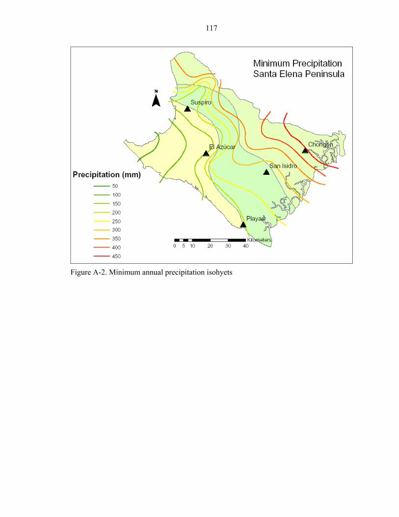
117
Figure A-2. Minimum annual precipitation isohyets

118
Figure A-3. Average annual precipitation isohyets

119
Figure A-4. Complete map of soils in the Santa Elena Peninsula
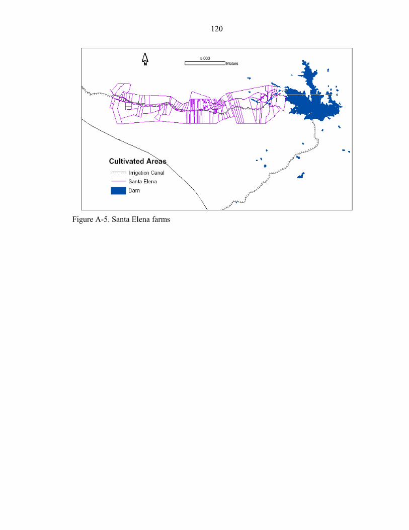
120
Figure A-5. Santa Elena farms
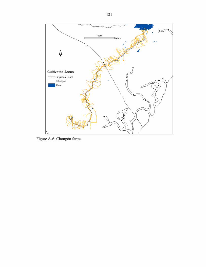
121
Figure A-6. Chongón farms
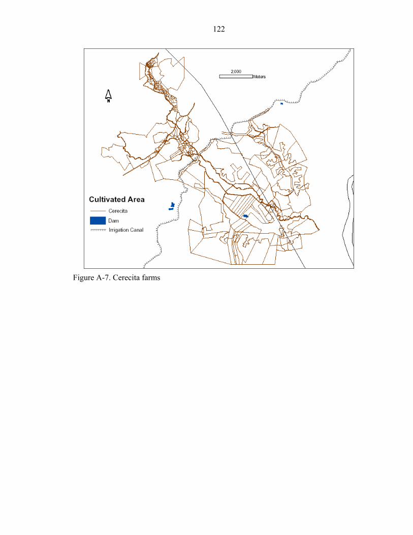
122
Figure A-7. Cerecita farms

123
Figure A-8. Azúcar-Rio Verde farms

APPENDIX B AVERAGE WEATHER DATA
Table B-1. Available weather data sets Available Weather Data Sets
Weather station Periods Chongón 1991-2000 El Azúcar 1966-1991 1995-2000 Playas 1962-1978 1995-2000 San Isidro 1991-1998 Suspiro 1962-1969 1991-1996
Chongón weather station is located in the CEDEGE experimental station at 24 m of
elevation. The parameters registered in this station are temperature, relative humidity,
wind speed, hour of light, precipitation, and evaporation, this data is different from all the
others in the Santa Elena Peninsula since this station is close to Guayaquil where more
rainfall is found.
Playas weather station is located near to the coastal line. Its climate is influenced by
the winds coming from the ocean. The evaporation is highest on this station, and the
precipitation is scarce.
El Azúcar weather station is located in the CEDEGE research station in El Azúcar.
This station started its operation again in 2000. The parameters collected as the same as
those shown in this table that collects historical data for this station.
El Suspiro and San Isidro were under CEDEGE control but they are not operational
at this moment.
124

Table B-2. Chongón weather station Chongón 1991 - 2000
LATITUDE: 2° 14' S LONGITUDE: 80° 04' E ELEVATION: 24 m TEMPERAT
URE (°C) RELATIVE HUM. (%)
WIND (m/sec) LIGHT PRECIP EVAP MONTH
Avg.
Avg. Day Night H/month mm mmJanuary 27.0 82 0.9 1.0 102.4 58.3 71.5
February 27.2
87 0.6 0.5 79.7 238.5 69.7March 28.1 86 0.7 0.5 99.9 220.2 82.8April 27.5 86 0.7 0.4 126.8 114.7 80.1May 26.9 84 0.7 0.5 119.0 68.9 104.8June 26.5 81 0.9 0.7 81.8 4.2 99.3July 24.8 81 1.0 0.7 86.6 0.0 97.4
August 24.9 77 1.1 1.0 134.2 1.1 107.7September 25.3 78 1.2 1.0 89.4 1.7 88.7
October 26.4 75 1.0 1.0 120.2 4.0 90.5November 26.5 73 1.2 1.0 116.4 1.1 83.3December 28.0 71 1.0 1.3 74.7 51.5 75.0
125
• CEDEGE (2001). N/D: no data

Table B-3. Playas weather station Playas 1963 – 1978
LATITUDE: 2° 37' S LONGITUDE: 80° 23' E ELEVATION: 41m
MONTH TEMPERATURE (°C)
RELATIVE HUM. (%)
WIND (m/sec) LIGHT PRECIP EVAP.
Avg Avg Day Night h/day mm mm January 25.7 77 3.1 N/D 5.3 97.5 N/D February 26.3 78 3.1 N/D 5.2 83.9 N/D March 26.6 79 2.9 N/D 5.8 135.7 N/D April 26.2 77 3.1 N/D 6.5 38.7 N/D May 25.2 79 3.4 N/D 5.7 10.3 N/D June 24.0 79 3.4 N/D 4.2 5.6 N/D July 24.9 80 3.7 N/D 3.6 2.1 N/D
August 22.4 79 4.2 N/D 3.6 1.2 N/D September 22.3 78 4.3 N/D 3.9 2.5 N/D
October 22.7 78 3.6 N/D 3.6 2.8 N/D November 23.2 79 4.1 N/D 4.8 0.9 N/D December 24.3 78 3.9 N/D 6.1 3.2 N/D
126
• CEDEGE (2001). N/D: no data

Table B-4. El Azúcar weather station El Azúcar 1974 - 1991
LATITUDE: 2°15´S LONGITUDE: 80°35´W ELEVACION: 50m
MONTH TEMP. (°C) RELATIVE HUM. (%)
WIND (m/sec) LIGHT PRECIP. EVAP.
Avg Avg. Night Day h/mo mm mm January 25.8 89 N/D 1.4 98.3 49.8 151.8 February 25.9 89 N/D 1.2 100.3 71.3 118.8 March 26.2 88 N/D 1.5 151.5 63.3 138.4 April 26.0 89 N/D 1.2 120.2 20.8 139.2 May 25.3 88 N/D 1.4 139.6 2.2 144.7 June 23.8 89 N/D 1.5 87.4 1.1 115.4 July 23.3 90 N/D 1.6 82.6 0.4 107.7
August 22.9 89 N/D 1.6 89.9 0.2 134.4 September 23.5 90 N/D 1.6 100.6 0.3 137.2
October 23.5 90 N/D 1.7 67.1 1.0 136.0 November 24.1 89 N/D 1.9 85.7 4.4 153.6 December 25.2 89 N/D 1.5 126.6 8.1 149.6
127

Table B-5. San Isidro weather station San Isidro 1991 - 1998
LATITUDE: 2°25´S LONGITUDE: 80°58´W ELEVACION: 35m
MONTH TEMP. (°C) RELATIVE HUM. (%)
WIND (m/sec) LIGHT PRECIP. EVAP.
Avg Avg. Night Day h/mo mm mm January 26.4 87 0.2 0.5 N/D 95 99 February 26.4 90 0.1 0.3 N/D 313 67 March 26.5 91 0.1 0.2 N/D 419 100 April 26.6 90 0.1 0.3 N/D 192 84 May 26.1 87 0.3 0.4 N/D 108 87 June 25.5 86 0.4 0.5 N/D 10 89 July 25.6 86 0.5 0.5 N/D 109 90
August 25.2 86 0.5 0.6 N/D 0 71 September 25.3 86 0.6 0.8 N/D 36 87
October 25.2 84 0.8 0.8 N/D 20 97 November 25.6 85 0.4 0.8 N/D 175 94 December 26.0 85 0.9 0.7 N/D 263 82
128
• CEDEGE (2001). N/D: no data

Table B-6. Suspiro weather station Suspiro 1962-1969/1991-1996
LATITUDE: 2°15´S LONGITUDE: 80°35´W ELEVACION: 35m
MONTH TEMP. (°C) RELATIVE HUM. (%)
WIND (m/sec) LIGHT PRECIP. EVAP.
Avg Avg. Night Day h/mo mm mm January 25.9 80 N/D N/D N/D 39 161 February 26.1 81 N/D N/D N/D 125 130 March 26.4 81 N/D N/D N/D 92 173 April 26.0 77 N/D N/D N/D 18 131 May 25.2 82 N/D N/D N/D 11 151 June 23.2 88 N/D N/D N/D 12 117 July 22.0 90 N/D N/D N/D 17 77
August 21.4 89 N/D N/D N/D 14 59 September 21.7 88 N/D N/D N/D 6 71
October 21.6 91 N/D N/D N/D 38 96 November 21.9 90 N/D N/D N/D 10 121 December 24.5 82 N/D N/D N/D 26 164
129
• CEDEGE (2001). N/D: no data

APPENDIX C CROPWAT REFERENCE EVAPOTRANSPIRATION TABLES
Table C-1. Reference evapotranspiration Chongón 11/1/2002 CropWat 4 Windows Ver 4.3 *********************************************************************** Climate and ETo (grass) Data (based on 9 years of data) *********************************************************************** Data Source: C:\CROPWATW\CLIMATE\CHONGON.PEM ----------------------------------------------------------------------- Country : Ecuador Station : Chongón Altitude: 24 meter(s) above M.S.L. Latitude: -2.23 Deg. (South) Longitude: 80.07 Deg. (East) ----------------------------------------------------------------------- Month MaxTemp MiniTemp Humidity Wind Spd. SunShine Solar Rad. ETo (deg.C) (deg.C) (%) (Km/d) (Hours) (MJ/m2/d(mm/d) ----------------------------------------------------------------------- January 31.2 19.0 79.5 77.8 3.3 14.3 3.29 February 30.7 19.1 80.1 51.8 2.8 13.9 3.08 March 30.7 19.3 79.2 60.5 3.2 14.6 3.24 April 31.0 19.5 79.6 60.5 4.2 15.5 3.35 May 30.5 19.3 78.3 60.5 3.8 13.9 3.02 June 30.4 18.7 78.9 77.8 2.7 11.8 2.77 July 30.8 18.5 78.9 86.4 2.8 12.1 2.90 August 30.8 20.0 79.0 95.0 4.3 15.1 3.43 September 30.8 19.3 79.5 103.7 3.0 13.9 3.34 October 30.6 19.8 78.2 86.4 3.9 15.5 3.52 November 30.8 19.9 79.1 103.7 3.9 15.2 3.54 December 30.4 19.3 78.1 86.4 2.4 12.7 3.06 ----------------------------------------------------------------------- Average 30.7 19.3 79.0 79.2 3.4 14.1 3.21 ----------------------------------------------------------------------- Pen-Mon equation was used in ETo calculations with the following values for Angstrom's Coefficients: a = 0.25 b = 0.5 *********************************************************************** C:\CROPWATW\REPORTS\CHONGON2.TXT
130

131
Table C-2. Reference evapotranspiration El Azúcar 11/1/2002 CropWat 4 Windows Ver 4.3 *********************************************************************** Climate and ETo (grass) Data Azúcar (based on 30 years of data) *********************************************************************** Data Source: C:\CROPWATW\CLIMATE\AZUCAR.PEM ----------------------------------------------------------------------- Country : Ecuador Station : Azúcar Altitude: 35 meter(s) above M.S.L. Latitude: -2.25 Deg. (South) Longitude: 80.58 Deg. (East) ----------------------------------------------------------------------- Month MaxTemp MiniTemp Humidity Wind Spd. SunShine Solar Rad. ETo (deg.C) (deg.C) (%) (Km/d) (Hours) (MJ/m2/d)(mm/d) ----------------------------------------------------------------------- January 31.5 21.3 81.4 121.0 3.2 14.1 3.45 February 31.4 21.4 82.5 103.7 3.6 15.1 3.53 March 31.9 21.4 83.4 129.6 4.9 17.2 3.98 April 32.2 20.6 82.3 103.7 4.0 15.2 3.57 May 30.6 20.9 81.9 121.0 4.5 14.9 3.40 June 29.4 19.0 84.9 129.6 2.9 12.1 2.84 July 28.8 19.3 87.2 138.2 2.7 12.0 2.74 August 28.1 18.7 88.3 138.2 2.9 13.1 2.86 September 28.0 19.0 88.8 138.2 3.4 14.5 3.08 October 29.5 19.0 87.5 146.9 2.2 12.9 3.05 November 28.4 19.0 87.5 164.2 2.9 13.7 3.09 December 30.5 20.1 85.9 129.6 4.1 15.3 3.45 ----------------------------------------------------------------------- Average 30.0 20.0 85.1 130.3 3.4 14.2 3.25 ----------------------------------------------------------------------- Pen-Mon equation was used in ETo calculations with the following values for Angstrom's Coefficients: a = 0.25 b = 0.5 *********************************************************************** C:\CROPWATW\REPORTS\AZUCAR2.TXT
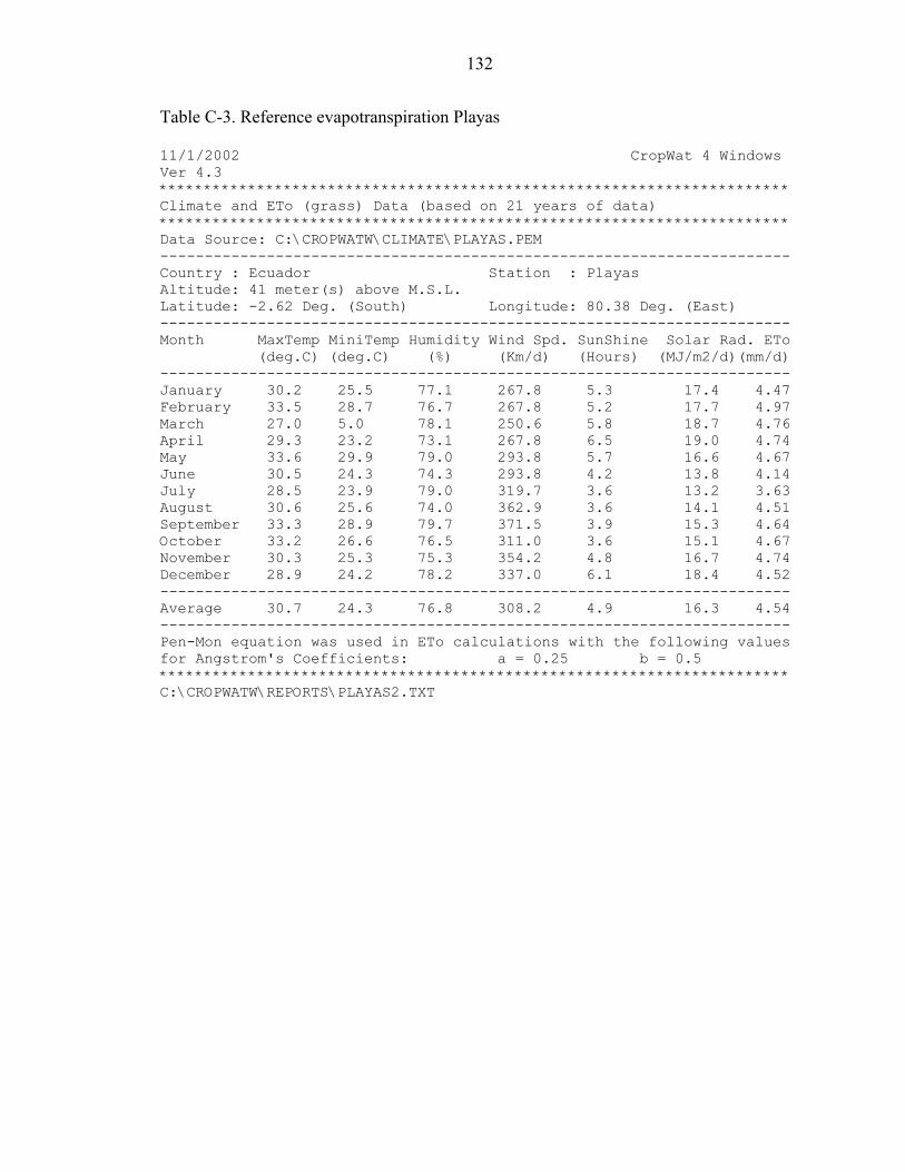
132
Table C-3. Reference evapotranspiration Playas 11/1/2002 CropWat 4 Windows Ver 4.3 *********************************************************************** Climate and ETo (grass) Data (based on 21 years of data) *********************************************************************** Data Source: C:\CROPWATW\CLIMATE\PLAYAS.PEM ----------------------------------------------------------------------- Country : Ecuador Station : Playas Altitude: 41 meter(s) above M.S.L. Latitude: -2.62 Deg. (South) Longitude: 80.38 Deg. (East) ----------------------------------------------------------------------- Month MaxTemp MiniTemp Humidity Wind Spd. SunShine Solar Rad. ETo (deg.C) (deg.C) (%) (Km/d) (Hours) (MJ/m2/d)(mm/d) ----------------------------------------------------------------------- January 30.2 25.5 77.1 267.8 5.3 17.4 4.47 February 33.5 28.7 76.7 267.8 5.2 17.7 4.97 March 27.0 5.0 78.1 250.6 5.8 18.7 4.76 April 29.3 23.2 73.1 267.8 6.5 19.0 4.74 May 33.6 29.9 79.0 293.8 5.7 16.6 4.67 June 30.5 24.3 74.3 293.8 4.2 13.8 4.14 July 28.5 23.9 79.0 319.7 3.6 13.2 3.63 August 30.6 25.6 74.0 362.9 3.6 14.1 4.51 September 33.3 28.9 79.7 371.5 3.9 15.3 4.64 October 33.2 26.6 76.5 311.0 3.6 15.1 4.67 November 30.3 25.3 75.3 354.2 4.8 16.7 4.74 December 28.9 24.2 78.2 337.0 6.1 18.4 4.52 ----------------------------------------------------------------------- Average 30.7 24.3 76.8 308.2 4.9 16.3 4.54 ----------------------------------------------------------------------- Pen-Mon equation was used in ETo calculations with the following values for Angstrom's Coefficients: a = 0.25 b = 0.5 *********************************************************************** C:\CROPWATW\REPORTS\PLAYAS2.TXT

133
Table C-4. Reference evapotranspiration San Isidro 11/1/2002 CropWat 4 Windows Ver 4.3 *********************************************************************** Climate and ETo (grass) Data (based on 7 years of data) *********************************************************************** Data Source: C:\CROPWATW\CLIMATE\SNISIDRO.PEM ----------------------------------------------------------------------- Country : Ecuador Station : San Isidro Altitude: 35 meter(s) above M.S.L. Latitude: -2.25 Deg. (South) Longitude: 80.58 Deg. (East) ----------------------------------------------------------------------- Month MaxTemp MiniTemp Humidity Wind Spd. SunShine Solar Rad. ETo (deg.C) (deg.C) (%) (Km/d) (Hours) (MJ/m2/d)(mm/d) ----------------------------------------------------------------------- January 31.0 20.2 85.3 43.2 4.3 15.8 3.32 February 31.3 20.7 85.3 25.9 4.2 16.1 3.36 March 31.4 20.4 85.8 17.3 4.8 17.1 3.50 April 31.4 20.9 85.6 25.9 5.5 17.5 3.56 May 31.3 20.9 85.1 34.6 4.7 15.2 3.13 June 31.5 20.8 84.8 43.2 3.2 12.5 2.71 July 31.2 20.1 85.2 43.2 2.6 11.9 2.60 August 31.7 20.5 85.1 51.8 2.6 12.6 2.83 September 31.3 20.5 85.0 69.1 2.9 13.8 3.11 October 31.5 20.9 84.7 69.1 2.6 13.5 3.10 November 31.4 20.8 84.7 69.1 3.8 15.1 3.34 December 31.7 20.6 84.5 60.5 5.1 16.8 3.59 ----------------------------------------------------------------------- Average 31.4 20.6 85.1 46.1 3.9 14.8 3.18 ----------------------------------------------------------------------- Pen-Mon equation was used in ETo calculations with the following values for Angstrom's Coefficients: a = 0.25 b = 0.5 *********************************************************************** C:\CROPWATW\REPORTS\ISIDRO2.TXT

134
Table C-5. Reference evapotranspiration Suspiro 11/1/2002 CropWat 4 Windows Ver 4.3 *********************************************************************** Climate and ETo (grass) Data (based on 13 years of data) *********************************************************************** Data Source: C:\CROPWATW\CLIMATE\SUSPIRO.PEM ----------------------------------------------------------------------- Country : Ecuador Station : Suspiro Altitude: 35 meter(s) above M.S.L. Latitude: -2.25 Deg. (South) Longitude: 80.58 Deg. (East) ----------------------------------------------------------------------- Month MaxTemp MiniTemp Humidity Wind Spd. SunShine Solar Rad. ETo (deg.C) (deg.C) (%) (Km/d) (Hours) (MJ/m2/d)(mm/d) ----------------------------------------------------------------------- January 31.6 20.3 75.3 164.2 3.2 14.1 3.86 February 31.3 21.4 75.6 146.9 3.6 15.1 3.88 March 32.1 21.0 78.3 146.9 4.9 17.2 4.20 April 31.7 20.2 77.0 155.5 4.0 15.2 3.90 May 30.4 21.4 77.0 129.6 4.5 14.9 3.54 June 28.8 19.3 78.3 112.3 2.9 12.1 2.88 July 27.9 18.6 84.7 86.4 2.7 12.0 2.59 August 26.2 17.9 88.0 129.6 2.9 13.1 2.70 September 25.8 17.0 87.3 121.0 3.4 14.5 2.92 October 25.5 17.9 87.5 129.6 2.2 12.9 2.69 November 26.3 18.3 86.3 86.4 2.9 13.7 2.80 December 30.0 20.2 83.5 167.0 4.1 15.3 3.58 ----------------------------------------------------------------------- Average 29.0 19.5 81.6 131.3 3.4 14.2 3.30 ----------------------------------------------------------------------- Pen-Mon equation was used in ETo calculations with the following values for Angstrom's Coefficients: a = 0.25 b = 0.5 *********************************************************************** C:\CROPWATW\REPORTS\SUSPIRO2.TXT

135
Figure C-1. Surface maps used to create a reference evapotranspiration map

136
Table C-6. Open water evaporation values per canal
Month Chongón-Cerecita
(m3) Cerecita-Playas
(m3) Chongón-Sube y
Baja (m3) Azúcar-Rio Verde (m3)
January 1064 528 531 740 February 1037 565 517 725 March 1085 560 541 792 April 1112 563 555 759 May 990 529 494 705 June 882 465 440 616 July 885 423 441 619 August 1008 498 502 690 September 1038 526 518 705 October 1066 527 531 721 November 1107 548 552 728 December 1070 550 534 714
Table C-7. Open water evaporation from dams
Month Chongón (m3) El Azúcar (m3) De Cola (m3)
January 90,886 50,456 2,324 February 85,085 51,626 2,584 March 89,505 58,208 2,475 April 92,544 52,211 2,465 May 83,428 49,725 2,428 June 76,521 41,535 2,153 July 80,113 40,073 1,888 August 94,754 41,828 2,345 September 92,268 45,045 2,413 October 97,240 44,606 2,428 November 97,793 45,191 2,465 December 84,533 50,456 2,350

APPENDIX D ECOCROP SELECTION CRITERIA TABLES
The information in ECOCROP permits the identification of 1,710 plant species
whose most important climate and soil requirements match the information on soil and
climate entered by the user. It also permits the identification of plant species for certain
uses. ECOCROP can be used as a library of crop environmental requirements and it can
provide plant species attribute files on crop environmental requirements to be compared
with soil and climate maps in Agro-ecological zoning (AEZ) databases or Geographical
Information System (GIS) map-based display.
A list of 60 crops was selected as potential crops for the SEP following workshops
and studies conducted by ESPOL and CEDEGE (2001). Following parameters were
considered:
• Crops actually being grow in the Santa Elena Peninsula • Market analysis for these crops • Ecology and adaptability to the zone • Discussion with the agricultural producers
From the list of 60 crops, following a process of elimination using ECOCROP, expert
advises from international market consultants, and producers a final list of 20 crops was
produced. Thirteen crops from that list are used to calculate water use in this project. In
this section the output given by ECOCROP is presented. These 13 crops were selected
because were considered the ones with better economical future.
137

Citrullus lanatus Herb. Annual Industry Commercial ND ND
C. reticulata Tree Perennial Fruit Garden, commercial 60 365
138
ECOCROP SELECTION CRITERIA (PRODUCTION)
DESCRIPTION CYCLE (days) SELECTED
CROPS FORM TYPE USES PRODUCTION SYSTEM MIN MAX
Psidium guajava L. Bush Perennial Fruit, lumber ND 150 365
Abelmoschus spp. Herb. Annual Vegetable ND 50 180 Algarrobo Bush, tree Perennial Medicine. Aromatic, Industry ND 210 365
Ficus carica L. Bush, tree Perennial Fruit, Medicine. Aromatic, Industry Garden 120 300
Cucurbita spp. Climbing Annual Fruit, Medicine. Aromatic, Industry, Forages, Vegetable Garden, commercial 80 140
Annona cherimola Bush, tree Perennial Fruit Garden, commercial 210 270 Anacardium occidentale Bush, tree Perennial Fruit, Medicine, Industry ND 190 260
C. sinensis Tree Perennial Fruit Commercial 180 365 Aloe spp. Herb. Perennial Medicine, Industry Garden 120 150
Lycopersicon esculentum Herb. Annual Aromatic, Industry, Forages,
Vegetable ND 70 150
Carica papaya L. Herb. Perennial Fruit, Medicine, Aromatic Garden, commercial 330 365
Cucumis sativus Herb. Annual Fruit, Medicine. Aromatic, Industry, Vegetable Garden, commercial 40 180
Persea spp. Tree Perennial Fruit, lumber ND ND ND Climbing, Fruit, Medicine. Aromatic,

139
Piper nigrum L. Climbing Perennial Medicine, Aromatic ND 180 270 Allium sativum L. Herb. Biannual Vegetable, Medicine. Aromatic ND ND ND Ananas comosus
Merr. Herb. Perennial Fruit ND 330 365
Cucumis melo L. Herb., Climbing Annual Fruit, Industry ND 50 120
Vitis spp. Bush, Climbing Perennial Fruit, Medicine, Industry Commercial 160 270
C. aurantifolia Tree Perennial Fruit, Aromatic ND ND ND Asparagus
officinalis L. Herb. Perennial Vegetable, Medicine, Industry Commercial 210 270
Allium cepa Herb. Biannual Vegetable, Medicine, Industry Garden, commercial 85 175 Musa spp. Herb. Perennial Fruit ND ND ND
Capsicum spp. ND ND ND ND ND ND

140
ECOCROP SELECTION CRITERIA (SOIL) SOIL THICKNESS
(cm) SOIL TEXTURE SOIL pH
OPTIMUM ABSOLUTE SELECTED
CROPS OPTIM ABSOLT OPTIMUM ABSOLUTE
MIN MAX MIN MAX Psidium guajava L. 50-150 20-50 Medium, organic Heavily, medium, light 5.5 7.5 4 8.5
Abelmoschus spp. 20-50 20-50 Heavily, medium, light, organic Heavily, medium, light 5.5 7 4.5 8.7
Algarrobo 20-50 20-50 Medium, light Medium, light 6 7.5 5 9 Ficus carica L. >150 50-150 Medium Heavily, medium, light 6 7 4.3 8.6
Cucurbita spp. >150 20-50 Heavily, medium, light, organic Heavily, medium, light 5.5 7.5 5 8.5
Annona cherimola >150 20-50 Medium, light Heavily, medium, light 7 8 4.3 8.5 Anacardium occidentale >150 50-150 Medium, light Heavily, medium, light 4.5 6.5 3.8 8.7
C. sinensis 150 50-150 Medium, light Heavily, medium, light 5 6 4 8.3 Aloe spp. 50-150 20-50 Light Medium, light 6.5 7 6 7.5
Lycopersicon esculentum 20-50 20-50 Medium, organic Heavily, medium, light 5.5 6.8 5 7.5
Carica papaya L. >150 50-150 Medium, organic Heavily, medium, light 5.5 7 4.5 8
Cucumis sativus 50-150 20-50 Medium, organic Heavily, medium, light 6 7.5 4.5 8.7
Persea spp. >150 >150 Medium Medium 5 5.8 4.5 7 Citrullus lanatus >150 50-150 Medium Light 6 7 5.5 7.5

141
C. reticulata >150 50-150 Medium, light Heavily, medium, light 6 6.8 5.5 8.3
Piper nigrum L. >150 50-150 Heavily, medium Heavily, medium, light 6 7 5 7.5
Allium sativum L. 50-150 20-50 Medium, light Heavily, medium, light 6 6.6 5 8.5
Ananas comosus Merr. 50-150 20-50 Medium, light Heavily, medium, light 4.5 8 3.5 9
Cucumis melo L. 50-150 50-150 Medium, organic Heavily, medium, light 6 7.5 5 8.7
Vitis spp. >150 20-50 Medium, organic Heavily, medium, light 5.5 7.5 4.5 8.5
C. aurantifolia 50-150 20-50 Medium, light Heavily, medium, light 5.5 6.5 5 7.5 Asparagus
officinalis L. 50-150 50-150 Medium, organic Medium, light 6 6.7 4.5 8.2
Allium cepa 50-150 20-50 Medium, organic Organic 6 7 4.3 8.3
Musa spp. ND ND ND ND ND ND ND ND
Capsicum spp. ND ND ND ND ND ND ND ND

C. reticulata 0 35 0 45 2300 THS, StSA, SbH, SSV, SSI Piper nigrum L. 0 15 0 20 2000 THS, TH
142
ECOCROP SELECTION CRITERIA (CLIMATE II)
LATITUD (decimal degrees) ELEVATION (m)
OPTIMUM ABSOLUTE ABSOLUTE SELECTED
CROPS
MIN MAX MIN MAX MAX
CLIMATIC ZONE
Psidium guajava L. 0 20 0 35 2000 THS, TH, StSa, SbH, SSV, SSI Abelmoschus spp. 0 35 0 40 1000 THS, TH, StSa, SbH, SSV, SSI
Algarrobo 27 42 25 45 1000 StSa, SbSV, TO Ficus carica L. 30 50 25 53 1200 THS, TH, StSa, SbH, SSV; SSI, TO, TC, THI, TSI Cucurbita spp. 10 20 0 50 2000 THS, TH, StSa, SbH, SSV; SSI, TO, TC, THI, TSI
Annona cherimola 0 15 0 25 1000 THS, TH, SSV Anacardium occidentale 0 25 0 30 1200 THS, StSa, SSV, SSI
C. sinensis 0 40 0 40 2100 THS, TH, StSa, SbH, SHV, SSI Aloe spp. 20 40 20 40 2000 StSa, SbSV
Lycopersicon esculentum 0 0 0 0 2400 THS; TH; StSr, SbH, SSV, SSI, TO, TC, THI, TSI
Carica papaya L. 0 30 0 32 2100 THS, TH Cucumis sativus 0 40 0 40 2000 THS; TH; StSr, SbH, SSV, SSI, TO, TC, THI, TSI
Persea spp. 0 42 0 42 2800 THS, TH Citrullus lanatus 20 43 10 43 1000 THS, TH, SbH, SHV, TO

143
Allium sativum L. 0 60 0 60 2200 THS; TH; StSr, SbH, SSV, SSI, TO, TC, THI, TSI Ananas comosus
Merr. 0 25 0 33 1800 THS, TH, SbH
Cucumis melo L. 0 0 0 0 1000 THS; TH; StSr, SbH, SSV, SSI, TO, TC, THI, TSI Vitis spp. 20 45 0 50 2000 THS; StSr, SSV, TO, TC
C. aurantifolia ND ND ND ND ND THS Asparagus
officinalis L. 0 60 0 60 2600 THS; TH; StSr, SbH, SSV, SSI, TO, TC, THI, TSI
Allium cepa 0 60 0 60 2000 THS; TH; StSr, SbH, SSV, SSI, TO, TC, THI, TSI Musa spp. ND ND ND ND ND ND
Capsicum spp. ND ND ND ND ND ND

Cucumis sativus 18 32 6 38 1000 1200 400 4300 High
luminosityHigh
luminosityHigh
luminosity Open sky
144
ECOCROP SELECTION CRITERIA (CLIMATE I) TEMPERATURE ( C) PRECIPITATION (mm) RADIATION
OPTIMUM ABSOLUTE OPTIMUM ABSOLUTE OPTIMUM ABSOLUTE SELECTED CROPS
MIN MAX MIN MAX MIN MAX MIN MAX MIN MAX MIN MAX Psidium
guajava L. 20 33 10 45 1000 3000 400 5000 High luminosity Open sky High
luminosity Cloudy sky
Abelmoschus spp. 20 30 12 35 600 1200 300 2500 Open sky Open sky High
luminosity Cloudy sky
Algarrobo 20 32 10 39 400 1000 200 2000 High luminosity Open sky High
luminosity Cloudy sky
Ficus carica L. 16 26 4 38 700 1500 300 2700 High luminosity Open sky High
luminosity Shadow
Cucurbita spp. 20 30 9 38 600 1000 450 2700 High luminosity
High luminosity
High luminosity Cloudy sky
Annona cherimola 23 30 11 41 800 1200 570 4000 High
luminosity Open sky High luminosity Cloudy sky
Anacardium occidentale 15 35 5 46 750 1600 400 4000 High
luminosityHigh
luminosityHigh
luminosity Open sky
C. sinensis 20 30 13 38 1200 2000 450 2700 High luminosity
High luminosity
High luminosity Open sky
Aloe spp. 18 26 10 30 500 600 300 800 High luminosity
High luminosity
High luminosity Cloudy sky
Lycopersicon esculentum 20 27 7 35 600 1300 400 1800 Open sky Open sky High
luminosity Cloudy sky
Carica papaya L. 21 30 12 44 1500 2500 1000 3000 High
luminosity Open sky High luminosity Cloudy sky

145
Persea spp. 18 40 12 45 500 2000 300 2500 High luminosity
High luminosity Open sky High
luminosityCitrullus lanatus 20 35 15 40 500 700 400 1800 Open sky High
luminosity Cloudy sky High luminosity
C. reticulata 23 34 12 38 1200 1800 300 4000 High luminosity
High luminosity
High luminosity Open sky
Piper nigrum L. 22 35 10 40 2500 4000 2000 5500 Open sky Shadow Open sky Shadow
Allium sativum L. 18 30 7 35 750 1600 500 2700 Open sky Open sky High
luminosity Cloudy sky
Ananas comosus
Merr. 21 30 10 36 800 2500 550 3500 Open sky Cloudy sky High
luminosity Shadow
Cucumis melo L. 18 30 9 35 1000 1300 900 2500 High
luminosityHigh
luminosityHigh
luminosity Open sky
Vitis spp. 18 30 10 38 700 850 400 1200 High luminosity
High luminosity
High luminosity Open sky
C. aurantifolia 20 28 12 32 1200 1500 750 2300 High luminosity
High luminosity
High luminosity Open sky
Asparagus officinalis L. 15 30 6 38 800 1200 500 4000 High
luminosityHigh
luminosityHigh
luminosity Cloudy sky
Allium cepa 12 25 4 30 350 600 300 2800 Open sky Open sky Cloudy sky High luminosity
Musa spp. ND ND ND ND ND ND ND ND ND ND ND ND
Capsicum spp. ND ND ND ND ND ND ND ND ND ND ND ND

146
ECOCROP SELECTION CRITERIA (FERTILITY/DRAINAGE)
FERTILITY SALINITY DRAINAGE SELECTED CROPS OPTIM ABSOLT OPTIM ABSOLT OPTIM ABSOLT SHORT DAYS
Psidium guajava L. High Low <4ds/m 4-10 ds/m good (dry season) good (dry season), excessive (very dry) <12 hr
Abelmoschus spp. High Moderate <4ds/m <4ds/m good (dry season) good (dry season) <12 hr
Algarrobo Moderate Low <4ds/m 4-10 ds/m good (dry season) good (dry season), excessive (very dry) <12 hr
Ficus carica L. Moderate Low <4ds/m 4-10 ds/m good (dry season) good (dry season), excessive (very dry)
<12hr, 12-14 hr, >14 hr
Cucurbita spp. High Low <4ds/m <4ds/m good (dry season) good (dry season) <12hr, 12-14 hr, >14 hr
Annona cherimola High Moderate <4ds/m <4ds/m good (dry season) good (dry season) <12 hr
Anacardium occidentale Moderate Low <4ds/m <4ds/m good (dry season) good (dry season),
excessive (very dry) <12hr, 12-14
hr, >14 hr
C. sinensis Moderate Low <4ds/m <4ds/m good (dry season) good (dry season) <12hr, 12-14 hr, >14 hr
Aloe spp. Moderate Low <4ds/m <4ds/m good (dry season) good (dry season),
excessive (very dry) <12 hr
Lycopersicon esculentum High Moderate
<4ds/m <4ds/m good (dry season) good (dry season) <12hr, 12-14 hr, >14 hr
Carica papaya L. High Moderate <4ds/m <4ds/m good (dry season) good (dry season),
excessive (very dry) <12hr, 12-14
hr, >14 hr

147
Cucumis sativus High Moderate <4ds/m <4ds/m good (dry season) good (dry season) <12hr, 12-14
hr, >14 hr Persea spp. Moderate Moderate <4ds/m <4ds/m good (dry season) good (dry season) ND
Citrullus lanatus High Low <4ds/m 4-10 ds/m good (dry season) good (dry season), excessive (very dry) >14 hr
C. reticulata High Moderate <4ds/m <4ds/m good (dry season) good (dry season),
excessive (very dry) <12 hr, 12-14
hr
Piper nigrum L. High Moderate <4ds/m <4ds/m good (dry season) good (dry season) <12hr, 12-14 hr, >14 hr
Allium sativum L. High Low <4ds/m <4ds/m good (dry season) good (dry season) >14 hr
Ananas comosus Merr. Moderate Moderate <4ds/m <4ds/m good (dry season) good (dry season) <12 hr
Cucumis melo L. Moderate Low <4ds/m <4ds/m good (dry season) good (dry season) <12hr, 12-14 hr, >14 hr
Vitis spp. Moderate Low <4ds/m <4ds/m good (dry season) good (dry season) <12hr, 12-14 hr, >14 hr
C. aurantifolia High Moderate <4ds/m <4ds/m good (dry season) good (dry season), excessive (very dry)
<12hr, 12-14 hr, >14 hr
Asparagus officinalis L. High Moderate <4ds/m 4-10 ds/m good (dry season) good (dry season) <12hr, 12-14
hr, >14 hr
Allium cepa Moderate Low <4ds/m 4-10 ds/m good (dry season) good (dry season) <12hr, 12-14
hr, >14 hr Musa spp. ND ND ND ND ND ND ND
Capsicum spp. ND ND ND ND ND ND ND

APPENDIX E TROPICAL CROPS
Aloe - Aloe spp.
Varieties: Aloe barbadensis, Aloe vera, Aloe arborensis, Aloe saponaria, Aloe
ferro, Aloe perryi.
Aloe is an evergreen perennial native to Europe and the Mediterranean. It escaped
cultivation and spread throughout the world. It is now found in deserts and jungles,
temperate and cold climates. Cultivation is fairly easy; the plant prefers light, sandy,
well-drained soil and a very sunny location (Atherton 1997).
Figure E-1. Aloe plantation, Santa Elena Peninsula
Asparagus - Asparagus officinalis L.
Varieties: Many new asparagus varieties are now available. All male hybrids are
more productive and do not produce seed which sprouts to become a weed (Phillips
1990).
Soils: Well-drained soils are a must for successful production, and very sandy soils
are preferred. Good drainage is important in control for crown rot disease of asparagus.
Commercial plantings of asparagus should not be made in soil that is heavier than a
sandy loam. An ideal site includes a sandy loam soil with good drainage and aeration,
148

149
water table below 1.2 m, and a pH of 6.8–7.5. Sites which retain standing water for more
than 8 hours after a heavy rain should be avoided (Mullen 1998).
Climate: Asparagus grows best when growing conditions include high light
intensity, warm days, cool nights, low relative humidity, and adequate soil moisture.
Compared to most other vegetables, asparagus is relatively winter hardy, with higher
heat, drought, and salt tolerances (Cantaluppi & Precheur 1993).
Spear initiation and root growth begin when the soil temperature is above 15
degrees C. Sandy soils warm earlier in the spring and encourage early spear production,
while irrigation cools the soil and retards spear production. Optimum productivity occurs
at 20–25 degrees C in the day and 15–20 degrees C at night. High daytime temperatures
during harvest will loosen the spear tip and develop fiber in the stem, both of which
reduce crop quality (Phillips 1990).
Cashew Nut - Anacardium occidentale
Cashew, a native of Brazil is a major crop for the tropics. It is a hardy crop, which
does well in areas considered relatively dry and marginal for many economic crops. The
crop also requires minimal care and skills from the farmer.
The cashew fruit consists of two distinct parts, a fleshy stalk in the form of a pear,
also called cashew apple, with a brilliant yellow or red skin, which can measure from 5 to
10 cm; and a nut of greybrownish color, in the shape of a kidney, which hangs from the
lower end of the stalk or "apple" and which is the true nut called cashew, very rich in
carbohydrates and Vitamin A. Of the stalk or "apple", juices, syrups, preserves, wine or
liquors are obtained. But its main commercial use is the cashew nut itself; shelled, roasted
and salted forming an ingredient as snack and the confectionery industry (delicacies,
chocolate, etc).

150
Climate: Cashew is hardy and drought resistant, and can grow better in areas with
rainfall between 500 mm and 1,500 mm per year. Cashew is well suited to a seasonally
wet/dry tropical climate. The area selected for cashew production should be frost-free.
Mean daily temperatures of less than 25 °C will limit the growth and productivity of
cashew trees. It is generally grown under rain fed conditions on soils of low fertility
(Rieger 1990).
Cucumber - Cucumis sativus
Cucumbers are a warm season crop and susceptible to frost damage. Low humidity
is favorable to cucumber production because of lower incidences of fruit and foliar
diseases. Extremely high temperatures may cause light green fruit color and bitterness in
many cucumber varieties.
Climate: Cucumbers are very tender, warm-season plants that grow best in
temperatures from 18.3 °C to 23.9 °C with a minimum temperature of 15.6 °C and a
maximum of 32.2 °C. Cucumber seeds germinate in soils at temperatures from 15.6 °C to
35 °C. Seeds do not germinate well at temperatures below 15.6 °C. Cucumber plants are
very susceptible to chilling injury in the field; prolonged temperatures below 12.8 °C
cause chilling injury to plants (pitting, water-soaked spots, and decay). Cucumber seed is
relatively vigorous, and stand establishment is not generally a problem if appropriate soil
preparation, temperature, and soil moisture conditions are met (Schrader 2002).
Soils: cucumbers are planted on a wide variety of soils. Lighter soils are usually
selected for earlier maturing fields. Cucumbers are a deep-rooted crop that grows best on
deep, fertile, well-drained soils. Very light soils that have excessive drainage and poor
moisture-holding potential should be avoided. Cucumbers are fairly salt tolerant.
Research has shown yield reduction of 10 percent starting at 3 dS/m (Schrader 2002).

151
Irrigation: cucumbers require frequent irrigation during the growing period. Too
little soil moisture, particularly when fruit is filling, can cause poorly shaped and curved
cucumbers. Fields should be maintained at or near field capacity to avoid plant stress and
to keep plants growing at a constant rate. The use of tensiometers to monitor soil
moisture and leaching is recommended.
Banana and Plantain - Musa spp.
Bananas and plantains belong to the family Musaceae, genus Musa. This family is
important not only for fruit production, but its other useful plants. Musa spp. have
provide man with food, clothing, tools, and shelter prior to recorded history.
Banana cultivars (Rieger 1990):
Gros Michel, (AAA genome) - Formerly the most widely cultivated banana in the
western hemisphere, it has now been phased out due to susceptibility to Panama disease
(Fusarium wilt). It has produced several clones and has been used as the parent for newer
cultivars. Male sterile.
Giant Cavendish, (AAA genome; syn.s “Mons Mari”, “Williams”, “Williams
Hybrid”, “Grand Naine”) Similar to “Gros Michel”, this is a medium-sized (3–5 m) plant
producing fairly large fruits with thicker skin to withstand bruising. Grown in Columbia,
Australia, Martinique, Hawaii, and Ecuador. Triploid; male and female sterile.
Dwarf Cavendish, (AAA genome) - A small (4–7 ft) plant bearing medium sized
fruit with thin skin. Grown in East Africa, South Africa, and the Canary Islands. Red
bananas are found in both Cavendish groups.
Lady finger, from the “Sucrier” group (AA genome), produces small (4–5 inch),
very sweet fruits with thin skin. Common in Latin America and Australia.

152
Plantain cultivars: “Maricongo”, “Common Dwarf”, “Pelipita”, “Saba” (generally
AAB, ABB, and BBB genomes) are the leading cultivars. In Florida, 'Macho' is grown as
a dooryard cultivar.
Figure E-2. Plantain in the Santa Elena Peninsula
Soils: Deep, well drained alluvial soils are best, but bananas can tolerate a wide
variety of soil conditions. Bananas require heavy fertilization for adequate yield
90–140 kg N/acre and up to 220-270 kg K/acre are used.
Climate: The banana is adapted to hot, wet, tropical lowlands. However, in South
and East Africa, banana cultivation may extend to 1500 m above sea level. Mean
temperature should be 25 °C, and about 100 mm rain/month are required, with dry
seasons no longer than 3 months. Frost kills plants to the ground, although the corm
usually survives (Rieger 1990).
Citrus fruits - Citrus spp.
The genus Citrus belongs to the Rutaceae family, sub-family Aurantoideae. This
family contains many edible species, some distantly related such as White Sapote
(Casimiroa edulis Llave & Lex.) and Wampee (Clausena lansium Skeels.).
The literature on citrus usually recognizes each economically important type as a
pecies, yielding the following (Rieger 1990):

153
C. aurantifolia (limes). The two main cultivars include the “Key” (syn. “Mexican”),
and “Tahiti” (syn. “Persian”). The latter is sometimes given species status as C. latifolia
(Tanaka) or Citrus x tahiti (C. Campbell). C. macrophylla is a lime-like fruit used as a
rootstock for lemons in California.
C. sinensis (the sweet oranges). This is a widely accepted name for this group,
containing many cultivars:
Navel oranges are unique in that cultivars have a secondary ovary embedded within
the usual ovary, giving a small fruitlet at the stylar end of the fruit at maturity; a fruit-
within-a-fruit. ‘Washington' is a major cultivar, but there are dozens.
C. reticulata (mandarin, satsuma, or tangerine). This is probably a "real" species.
Due to the success of breeding with these types, many cultivars and hybrids have been
produced or formed naturally, some erroneously given species status. Common cultivars
include: “Dancy”, “Clementine” or “Algerian”, “Owari” (a satsuma), “Cleopatra”
(common mandarin rootstock).
C. paradisi (the grapefruit). This is a relatively recent species (since 1700's) of
unknown origin. It probably derives from Caribbean “Forbidden Fruit”, and was
introduced to other places from there. Cultivars include: “Duncan”, “Marsh”, “Red-
blush”, and “Thompson” (syn. “Pink Marsh”). Hybrids include the tangelos and
citrumelos; the latter are used as rootstocks.
Soils: Citrus is adapted to a wide variety of soil types and conditions. Trees are
grown from almost pure sand, to organic muck, to loamy, heavy soils.
Climate: Citrus fruit obtains highest internal quality in subtropical humid climates.
However, with irrigation, it also grows well in Mediterranean climates, like California,

154
achieving the best external quality. In the tropics, citrus accumulates less sugar and acid,
and the peel usually remains green; also, bloom is not synchronized, so several stages of
maturity are present on the tree at any given time, causing some immature fruit to be
harvested (Rieger 1990).
Cold hardiness is the major limiting factor for citrus production in subtropical
areas. Fruit are killed by 30 minutes at –1 to –2 °C; larger fruit are more cold tolerant due
to greater thermal mass. Fruit freeze from the stem end to the button, and mildly frozen
fruit can be salvaged for juice. Leaves and stems are killed by a few minutes at –4 ° C to
–2° C, depending on stage of acclimation, species, and age of tissue. Citrus has no
chilling requirement, and does not attain a truly dormant state, but becomes quiescent at
temperatures below 13 °C (Rieger 1990).
Grapes - Vitis spp.
Grapes belong to the Vitaceae family. The genus Vitis is broadly distributed,
largely between 25 ° and 50 ° N latitude in eastern Asia, Europe, the Middle East, and
North America. Additionally, a few species of Vitis are found in the tropics: Mexico,
Guatemala, the Caribbean, and northern South America (Rieger 1990).
V. vinifera L., "Old world grape", "European grape". This is the major species of
grape, accounting for >90 % of world production. It was probably domesticated more
than 5000 years ago in the Middle East.
Figure E-3. Grapes

155
Soils: Grapes are adapted to a wide variety of soil conditions, from high pH and
salt, to acidic and clayey. Rootstocks allow adaptation to various soil situations.
However, deep, well-drained, light textured soils are best for wine grapes. Highly fertile
soils are unsuited to high quality wine production, since vigor and yield must be
controlled. Irrigation is detrimental to grape internal quality, and sometimes illegal for
wine grapes, but is beneficial for table and raisin grapes where high yields are desired.
Climate: Vinifera grapes can be generally characterized as requiring a long
growing season, relatively high summer temperatures, low humidity, a ripening season
free of rainfall, and mild winter temperatures.
Cold hardiness is a major limiting factor for vinifera grapes. Damage to primary
buds occurs at –18 to –23 °C, and trunks may be injured or killed below –23 °C.
Internal quality and hence wine quality is affected by summer temperature.
Humidity is another limiting factor for vinifera grape culture, due to disease
susceptibility. Grapes cannot tolerate high RH or rain during harvest (Rieger 1990).
Mango - Mangifera indica L.
The Mango, Mangifera indica L., is the most economically important fruit in the
Anacardiaceae (poison ivy family). Other important members of this family include
cashew and pistachio.
Figure E-4. Mangos

156
Cultivars: Hundreds of mango cultivars exist throughout the world. However, in
the western hemisphere, a few cultivars derived from a breeding program in Florida are
the most popular for international trade. Locally, many cultivars are used, and often
seedling trees are grown as a backyard food source.
Tommy Atkins, the most common mango in the US; medium sized (0.5 kg),
beautiful exterior but firm, finely fibrous, and low in flavor compared to others. This one
sells on eye-appeal.
Keitt, among the largest of major cultivars, about 0.75 kg (up to 1.2 kg).
Yellow/green skin color makes it less popular in the US, but the yellow-gold flesh is
fiberless and full-flavored.
Kent, red blush to skin, medium sized (0.55 kg), and relatively round. Fiberless,
rich-flavored flesh may have a turpentiny aftertaste.
Haden, the old, anthracnose-prone mainstay of Florida market; now replaced by
others, but 90 % of Hawaiian production, and grown in Ecuador (Guayaquil area) and
western Mexico. Small (< 0.5 kg) and relatively round, the red skin color is excellent
when grown in hot, sunny, dry climates. Firm flesh, almost fiberless.
Soils: Mango is adapted to many soil types, but it requires adequate drainage.
Excess fertility delays and reduces fruiting. Can be grown on soil with high pH. In
Florida, trees are grown on limestone gravel, and still do not develop iron deficiency.
Climate: Adapted to hot, tropical lowlands, to 1,000 m best quality in monsoon
climates, i.e., those with a distinct wet and dry season. Leaves and fruit are injured by
mild frost (–2 to –1°C), but wood is not killed unless temperatures drop to below –5' °C.

157
Onion - Allium cepa
Varieties: Onions are often grouped according to taste. The two main types of
onions are strong flavored (American) and mild or sweet (sometimes called European).
Each has three distinct colors yellow, white, and red. Generally, the American onion
produces bulbs of smaller size, denser texture, stronger flavor, and better keeping quality
than European types. Globe varieties tend to keep longer in storage (Riofrio & Wittmeyer
2000).
Figure E-5. Onion plantation and onions, Santa Elena Peninsula
Soils: Onions grow best in a loose, well-drained soil with high fertility and plenty
of organic matter. Avoid heavier soils such as clay and silt loams, unless they are
modified with organic matter to improve aeration and drainage. Onions are sensitive to
highly acid soils and grow best when the pH is between 6.2 and 6.8 (Riofrio & Wittmeyer
2000).
Climate: The onion is adapted to a wide range of temperatures and is frost-tolerant.
Best production is obtained when cool temperatures prevail over an extended period of
time, permitting considerable foliage and root development before bulbing starts. After
bulbing begins, high temperature and low relative humidity extending into the harvest
and curing period are desirable. A constant supply of adequate moisture is necessary for
best results. For onions started from plants, light mulch will help conserve moisture for
uniform growth (Riofrio & Wittmeyer 2000).

158
Papaya - Carica papaya L.
Papaya belongs to a small family of only two genera, the Caricaceae. This family is
often lumped into the Passifloraceae or passion fruit family by some. Carica papaya L.,
the papaya of commerce, is called "Paw-Paw" in some English-speaking countries;
however, this is not to be confused with the North American Annonaceous species
Asimina triloba Dunal. Carica pentagona Heilborn, the Babaco, is similar to papaya but
smaller (<3 m), producing 5-angled fruits reaching 0.3 m in length with few or no seeds
(Fruit Facts 2001).
Cultivars: “Solo” or “Sunrise solo”, Introduced to Hawaii from Barbados in 1911,
was the first major commercial cultivar. The name derives from the relatively small size
of the fruit, it can be eaten by one person, as opposed to the more common family-sized
fruits. Very high quality, smaller fruit; female plants produce, rounder, shallowly
furrowed fruits, hermaphrodites produce pear-shaped fruits. It has been used as a parent
in breeding programs, and produced newer cultivars such as “Kapoho solo”,
“Waimanalo”, “Higgins”, and “Wilder”. As of 1999, all of the “Solo” papaya grown in
Hawaii is transgenic; it has a gene inserted to confer resistance to papaya ringspot virus
(Rieger 1990).
Figure E-6. Papaya plantation in the Santa Elena Peninsula

159
Soils: Papaya growth is best in soils with pH 5.5–6.7, rich in organic matter.
However, fruits may be poor quality on highly fertile soils when vegetative growth is
excessive.
Climate: Papaya requires a tropical climate with high rainfall and temperature for
proper fruit maturation. Plants are damaged by frost, and completely killed by
temperatures close to –5 °C. High wind also causes damage by fruit loss or uprooting
(Fruit Facts 2001).
Pineapple - Ananas comosus Merr.
The pineapple, Ananas comosus Merr., is a member of the Bromeliaceae family, a
large, diverse family of 2000 species. The bromeliad family contains hundreds of taxa
used as ornamentals in greenhouses or sub-tropical areas: Billbergia, Vresia, Nidularium,
Pitcairnia, Tillandsia, Tillandsia usneoides is "spanish moss" native to the Gulf States.
Formerly, the pineapple was named A. sativus, Bromelia ananas, or B. comosus (Fruit
Facts 2001).
Cultivars: “Smooth Cayenne”, selected and cultivated by Venezuelan indians for
its large, juicy fruit and lack of spines on leaves. Subject to diseases, and having poor
shipping quality, it has been suplanted by superior sports in many areas. “Hilo” was
selected in Hawaii, and “St. Michael” in Azores. Used for canned slices and fresh market.
Fruit weight 2–5 kg.
“Red Spanish”, The major fresh cultivar in the Caribbean, the plants are spiny, but
disease resistant and fruits ship well. Roundish in shape, orange-red, 1.5–3 kg/fruit, and
fewer eyes than “Smooth” (Rieger 1990).
Soils: Well-drained sandy loams, with pH 4.5–6.5 are best. Fumigation is practiced
routinely, since nematodes are serious problems in most growing areas.

160
Climate: Pineapples are resticted to tropical lowlands, with temperatures of
18-35 °C and precipitation of 1,100 mm distributed in spring and fall. Humidity is
usually high.
Pineapple is relatively drought-tolerant, and can be grown in areas receiving as
little as 600 mm/yr. Alternatively, 3,800 mm/yr are tolerated if drainage is adequate.
If climate during ripening is too cool, fruit are too acid, and if climate is too warm,
fruit may be insipidly sweet.
Cherimoya - Annona cherimola
The cherimoya is regarded by many as being among the best of tropical fruits. The
cherimoya has a texture of a soft, non-gritty pear and a delicate, highly appealing fruit
flavor with little acidity. Cherimoyas usually are eaten fresh; however they are excellent
in ice cream and sherbets (Fruit Facts 2001).
Soils: The most critical soil requirement is that of good drainage. Sandy loam or
decomposed granite is preferred, but cherimoyas will succeed on many soil types with
pH 5 to 8 (Fruit Facts 2001).
Climate: All of the species grown for fruit require a tropical or semitropical
climate except for the pawpaw which is native to temperate North America. Moreover,
all but the cherimoya are better adapted to wet tropical conditions. The cherimoya’s
home is the highland tropics which are often characterized as areas of eternal spring with
temperatures seldom straying from the 15’s ° (C). There are wet and dry seasons with
typical annual rainfalls being about 1,200 mm (Fruit Facts 2001).
The cherimoya is adaptable to Mediterranean climates. In addition to San Diego
and Santa Barbara and Ventura counties in the United States, significant commercial
plantings have been made in Chile, Spain, Peru, Israel, New Zealand, Australia and Italy.

161
The cherimoya requires a relatively frost-free environment similar to lemons (short
periods of –2 °C for mature trees of hardy varieties). Some chilling seems beneficial (50
to 100 hours between 1 °C and 5 °C). However, a sunny location is needed since
sufficient heat is required to develop a good flavor (inland, protection from extremely hot
temperatures and dry winds is more important). In California most varieties do well
extending 2 to 8 km inland from the ocean. Further inland, care must be exercised in
selecting a variety that will do well. The cherimoya will not tolerate prolonged high
humidity, such as is encountered in Florida (Fruit Facts 2001).
Avocado - Persea spp.
Species: Guatemalan (Persea nubigena var. guatamalensis L. Wms.), Mexican (P.
americana var. drymifolia Blake), West Indian (P. americana Mill. var. americana).
Hybrid forms exist between all three types (National Department of Agriculture 2000).
Soil: Avocado trees like loose, decomposed granite or sandy loam best. They will
not survive in locations with poor drainage. The trees grow well on hillsides and should
never be planted in stream beds. They are tolerant of acid or alkaline soil (National
Department of Agriculture 2000).
Climate: The 3 best-known avocado races each has specific climatic requirements
as a result of adapting to their original environment.
West Indian cultivars originated in the humid, tropical lowlands of Central America
and are best adapted to continuous hot, humid conditions with a high summer rainfall.
Like all avocado cultivars they are, however, extremely sensitive to drought and do not
tolerate frost well (minimum temperature of 1.5 °C). The optimum temperature for
growth is 25 to 28 °C. The humidity should preferably be above 60 % (National
Department of Agriculture 2000).

162
The Mexican races originated in the cool, subtropical highland forests of Mexico
and mature trees can withstand temperatures of –4 to –5 °C. They should not be planted
in areas prone to frost in August and September, because flowers are damaged easily by
frost. A humidity range of 45 to 60 % should suffice. The optimum temperature for
growth is 20 to 24 °C (National Department of Agriculture 2000).
Guatemalan cultivars originated from the tropical highlands of Guatemala and
require a cool, tropical climate without any extremes of temperature or humidity. The
trees can withstand light frost, down to –2 °C, but the flowers are very sensitive to frost.
High temperatures of about 38 °C, especially if combined with low humidity, could cause
flower and fruit drop. A humidity level of 65 % or higher is required (National
Department of Agriculture 2000).
Tomato - Lycopersicon esculentum
Soils: A wide variety of soil textures are used for fresh-market tomato production.
Sandy soils are preferred for early plantings (Hochmuth 2001). This is because planting
can be done in sandy soils more easily during wet weather. Sand also warms more rapidly
in the spring, promoting early growth. Loam and clay loam soils, however, are generally
more productive than sand. Clay soil may be used, provided it is well drained and
irrigated with care (Tomato Production Guide for Florida 2002).
Climate: The tomato is a warm-season vegetable crop that is sensitive to frost at
any stage of growth. The optimum soil temperature for seed germination is 20 °C or
above; seed germination below 16 °C is very slow. Optimal production temperatures are
between 21 °C and 27 °C. These temperatures are ideal for vegetative growth, fruit set,
and development. With adequate soil moisture, tomato plants can tolerate temperatures in
excess of 38 °C, although fruit set is adversely affected. Tomato fruit development and

163
quality are reduced when day temperatures fall below 20 °C, and plants undergo chilling
injury when night temperatures fall below 10 °C (Tomato Production Guide for Florida
2002).
Melon (Cantaloupe) - Cucumis melo L
Soils: Melons prefer well-drained soils. Sandy or silt loams are sometimes selected
for the earliest crop. Heavier soils are preferred because of their greater water holding
capacity, which slows the onset of vine collapse. Beds should be left cloddy to allow
maturing melons to develop with minimal soil contact and good aeration (Mayberry
1996).
Cantaloupes grow best on soils that hold water well and have good air and water
infiltration rates. Soil should have a pH of 5.8 to 6.6. Cantaloupes are sensitive to cold
temperatures, and even a mild frost can injure the crop (Mayberry 1996).
Climate: The best average temperature range for cantaloupe production during the
growing season is between 20 °C and 30 °C; temperatures above 30 °C or below 15 °C
will slow the growth and maturation of the crop (Orzolek 2002).
Irrigation: Cantaloupes require a constant supply of moisture during the growing
season. However, excess water at any time during crop growth, especially as fruit reaches
maturity, can cause the fruit to crack, which will reduce crop yields and fruit quality
(Orzolek 2002).
Guava - Psidium guajava L
The place of origin of the guava is uncertain, but it is believed to be an area
extending from southern Mexico into or through Central America. It has been spread by
man, birds and other animals to all warm areas of tropical America and in the West Indies
(since 1526).

164
The guava is an evergreen tree reaching a height of 3–10 m. The trunk is slender
with a greenish-brown scaly bark which peels off in thin flakes. The white flowers are
either solitary or in groups of two or three, arising from the leaf axils of younger
branches. The fruit is round, ovoid or pear- shaped berry, 5 cm or more in diameter and
4–12 cm long. It has a thin greenish-yellow skin and a flesh of varying thickness which
may be white, yellow-pink or red. The outer layer of flesh is a finely granular pulp; the
inside is softer pulp with many small hard seeds. Some varieties are seedless. The flavor
is variable and is distinguished by a characteristic and penetrating musky aroma of
varying intensity.
Guava, a native of tropical America is well distributed throughout the tropics and
subtropics.
Soils: the guava is a hardy plant which grows in most soil types. Loam and alluvial
types of soil is most ideal. The guava will tolerate many soil conditions, but will produce
better in rich soils high in organic matter. They also prefer a well-drained soil in the pH
range of 5 to 7. The tree will take temporary water logging but will not tolerate salty
soils.
Although the guava can tolerate low moisture condition, availability of water constantly
will promote fast growth and leaf flushes. A warm, humid condition is most optimum for
guavas. Guavas have survived dry summers with no water, although they do best with
regular deep watering. The ground should be allowed to dry to a depth of several inches
before watering again. Lack of moisture will delay bloom and cause the fruit to drop.
Fig - Ficus carica L.
Climate: the fig grows best and produces the best quality fruit in Mediterranean
and dryer warm-temperate climates. Rains during fruit development and ripening can

165
cause the fruits to split. With extra care figs will also grow in wetter, cooler areas.
Diseases limit utility in tropical climates. Fully dormant trees are hardy to –4 °C to –5 °C,
but plants in active growth can be damaged at 0 °C. Figs require full sun all day to ripen
palatable fruits. Trees become enormous, and will shade out anything growing beneath.
The succulent trunk and branches are unusually sensitive to heat and sun damage, and
should be whitewashed if particularly exposed. Roots are greedy, traveling far beyond the
tree canopy. In areas with short (less than 120 days between frosts), cool summers,
espalier trees against a south-facing, light-colored wall to take advantage of the reflected
heat. In coastal climates, grow in the warmest location, against a sunny wall or in a heat
trap (Rieger 1990).
Irrigation: young fig tees should be watered regularly until fully established. Is
recommended to water mature trees deeply at least every one or two weeks. Desert
gardeners may have to water more frequently. Mulch the soil around the trees to conserve
moisture. Also, drought-stressed trees will not produce fruit and are more susceptible to
nematode damage. Recently planted trees are particularly susceptible to water deficits,
often runt out, and die (Rieger 1990).
Watermelon - Citrullus lanatus
Watermelon is a warm-season crop related to cantaloupe, squash, cucumber and
pumpkin.
Soils: most well drained soil, whether clayey or sandy, can be managed to produce
a good crop of watermelon. The best soils, however, are sandy loams that have not been
in cucurbit (cantaloupe, cucumber, squash, etc.) production for a minimum of five years
(Boyham 2001).

166
Irrigation: 250 mm of timely rains or irrigations on a deep, sandy soil produce a
good crop of watermelons. Growers with limited irrigation capabilities can often increase
yields with only one or two irrigations. Inadequate moisture at planting results in poor
and uneven emergence. Moisture shortage at bloom results in poor fruit set and
misshapen fruit. Moisture stress close to harvest greatly reduces melon size and results in
rapid vine decline. When irrigating, apply one to two inches of water (Roberts 2002).

167
B-Pepper 115.4 143.0 190.8 182.9 136.0 140.7 165.7 161.3
APPENDIX F IRRIGATION REQUIREMENTS
Table F-1. Chongón-San Isidro, 50% efficiency
Table F-2. San Isidro-Playas, 50% efficiency
Irrigation Requirement (mm) San Isidro-Playas, 50% irrigation
efficiency Month Jan Feb March April May June July Aug Sept Oct Nov Dec Avocado 116.6 137.3 157.1 146.0 117.2 127.7 134.1 129.1 Asparagus 113.3 140.8 160.8 108.4 Plantain 93.8 94.2 92.4 106.3 184.7 167.8 173.6 172.0 27.8 Citrus 131.3 131.9 129.4 123.5 154.7 108.8 105.6 105.7 88.3 115.0 118.8 103.8Grapes-T 75.0 75.3 73.9 70.6 91.1 99.8 132.0 137.5 143.7 150.3 146.5 81.7Mango 168.2 169.3 166.3 164.9 223.8 172.3 173.6 177.9 185.3 185.0 179.0 140.7Onion 136.0 140.7 165.7 163.3 68.4 Pineapple 90.5 74.8 55.4 53.0 31.9 Potato 106.1 165.3 212.5 186.7 46.0 Melon 98.2 158.4 186.2 163.0 Watermelon 97.3 151.4 177.3 158.6 S-Pepper 132.4 150.6 186.2 181.7
Irrigation Requirement (mm) Chongón-San Isidro, 50% irrigation
efficiency Month Jan Feb March April May June July Aug Sept Oct Nov Dec Avocado 94.8 111.0 126.4 117.9 112.3 106.1 112.8 109.4 Asparagus 95.2 119.3 136.5 91.7 Plantain 76.3 76.2 74.4 85.9 151.1 139.5 146.0 145.8 23.6 Citrus 106.8 106.7 104.1 99.8 126.5 90.5 88.8 89.6 93.2 97.3 100.1 87.2Grapes-T 61.0 60.9 59.5 57.0 74.5 83.0 111.1 116.5 121.9 127.3 123.4 68.6Mango 136.8 136.9 133.9 133.2 183.0 143.2 146.0 150.8 155.6 156.6 149.3 118.2Onion 111.3 116.9 139.4 138.4 58.1 Pineapple 73.7 60.5 44.6 42.8 28.7 Potato 86.2 133.9 171.1 150.8 37.4 Melon 83.2 134.4 157.5 137.3 Watermelon 82.4 103.0 150.0 133.6 S-Pepper 112.1 127.8 157.5 153.1 B-Pepper 93.9 115.6 153.6 147.8 111.3 116.9 139.4 136.6

168
Table F-3. Chongón-El Azúcar, 50% efficiency
Irrigation Requirement (mm) Chongón-El Azúcar, 70% irrigation
efficiency Month Jan Feb March April May June July Aug Sept Oct Nov Dec Avocado 96.1 113.7131.2 122.9 116.7108.9 114.1 108.9 Asparagus 96.4 119.0 134.5 92.3 Plantain 77.3 78.0 77.2 89.6 157.0143.2 147.6 145.2 23.3 Citrus 108.2 109.2108.0 104.1 131.4 92.9 89.8 89.2 91.9 95.5 98.5 86.5Grapes-T 61.8 62.4 61.7 59.5 77.5 85.2 112.2 116.0 120.2 124.7 121.5 67.8Mango 139.1 140.3138.8 138.9 190.2147.0 147.6 150.4 153.3 153.7 146.9117.3Onion 115.6120.0 140.9 137.8 57.4 Pineapple 74.6 61.9 46.3 44.6 14.4 Potato 87.5 137.3178.2 157.3 38.9 Melon 82.9 132.3 154.6 135.2 Watermelon 82.1 101.0 147.2 131.6 S-Pepper 111.8 125.8 154.6 153.2 B-Pepper 95.2 118.4159.4 154.1 115.6120.0 140.9 136.1
Table F-4. Chongón - San Isidro, 70% efficiency Irrigation Requirement (mm) Chongón-San Isidro, 70% irrigation efficiencyMonth Jan Feb March April May June July Aug Sept Oct Nov Dec Avocado 82.2 96.2 109.6 102.2 97.4 92.0 97.8 94.8 Asparagus 82.5 103.4 118.3 79.5 Plantain 66.1 66.0 64.4 74.5 131.0 120.9 126.5 126.3 20.4 Citrus 92.6 92.4 90.2 86.5 109.6 78.4 77.0 77.6 80.8 84.3 86.7 75.6Grapes-T 52.9 52.8 51.6 49.4 64.6 71.9 96.2 101.0 105.7 110.3 107.0 59.5Mango 118.5 118.7 116.0 115.4 158.6 124.1 126.5 130.7 134.8 135.7 129.4 102.4Onion 96.4 101.4 120.8 119.9 50.3 Pineapple 63.8 52.5 38.7 37.1 24.9 Potato 74.7 116.0 148.3 130.7 32.4 Melon 72.1 116.5 136.5 119.0 Watermelon 71.4 89.2 130.0 115.8 S-Pepper 97.2 110.8 136.5 132.7 B-Pepper 81.4 100.2 133.1 128.1 96.4 101.4 120.8 118.4

169
Table F-5. San Isidro-Playas, 70% efficiency Irrigation Requirement (mm) San Isidro-Playas, 70% irrigation efficiency Month Jan Feb March April May June July Aug Sept Oct Nov Dec Avocado 101.0 119.0 136.1 126.5 101.6 110.7 116.2 111.9 Asparagus 98.2 122.0 139.4 93.9 Plantain 81.3 81.6 80.1 92.1 160.1 145.5 150.4 149.1 24.1 Citrus 113.8 114.3 112.1 107.1 134.0 94.3 91.5 91.6 76.5 99.6 103.0 90.0Grapes-T 65.0 65.3 64.1 61.2 79.0 86.5 114.4 119.2 124.5 130.3 127.0 70.8Mango 145.8 146.8 144.1 142.9 193.9 149.4 150.4 154.2 160.6 160.3 155.1 121.9Onion 117.9 121.9 143.6 141.5 59.3 Pineapple 78.5 64.8 48.0 45.9 27.6 Potato 91.9 143.3 184.2 161.8 39.8 Melon 85.1 137.3 161.4 141.3 Watermelon 84.3 131.2 153.7 137.5 S-Pepper 114.8 130.5 161.4 157.5 B-Pepper 100.1 123.9 165.4 158.5 117.9 121.9 143.6 139.8
Table F-6. Chongón-El Azúcar, 70% efficiency Irrigation Requirement (mm) Chongón-El Azúcar, 70% irrigation efficiencyMonth Jan Feb MarchApril May June July Aug Sept Oct Nov Dec Avocado 83.3 98.5 113.7 106.5 101.2 94.4 98.8 94.4 Asparagus 83.6 103.1 116.5 80.0 Plantain 67.0 67.6 66.9 77.6 136.1 124.1 127.9 125.8 20.2 Citrus 93.8 94.6 93.6 90.2 113.9 80.5 77.8 77.3 79.6 82.7 85.4 75.0Grapes-T 53.6 54.1 53.5 51.5 67.1 73.8 97.3 100.6 104.1 108.0 105.3 58.8Mango 120.6 121.6 120.3 120.4 164.8 127.4 127.9 130.3 132.8 133.2 127.3 101.6Onion 100.2 104.0 122.1 119.4 49.7 Pineapple 64.7 53.6 40.1 38.6 12.5 Potato 75.8 119.0 154.4 136.3 33.7 Melon 71.9 114.7 134.0 117.2 Watermelon 71.2 87.5 127.6 114.0 S-Pepper 96.9 109.1 134.0 132.7 B-Pepper 82.5 102.6 138.1 133.5 100.2 104.0 122.1 117.9

170
Table F-7. Chongón-San Isidro, 90% efficiency Irrigation Requirement (mm) Chongón-San Isidro, 90% irrigation efficiencyMonth Jan Feb MarchApril May June July Aug Sept Oct Nov Dec
Avocado 69.5 81.4 92.7 86.5 82.4 77.8 82.7 80.2 Asparagus 69.8 87.5 100.1 67.3 Plantain 56.0 55.9 54.5 63.0 110.8 102.3 107.1 106.9 17.3 Citrus 78.3 78.2 76.4 73.2 92.8 66.3 65.1 65.7 68.4 71.3 73.4 63.9Grapes-T 44.8 44.7 43.6 41.8 54.7 60.9 81.4 85.4 89.4 93.4 90.5 50.3Mango 100.3 100.4 98.2 97.7 134.2 105.0 107.1 110.6 114.1 114.8 109.5 86.6Onion 81.6 85.8 102.2 101.5 42.6 Pineapple 54.0 44.4 32.7 31.4 21.1 Potato 63.2 98.2 125.4 110.6 27.4 Melon 61.0 98.5 115.5 100.7 Watermelon 60.4 75.5 110.0 98.0 S-Pepper 82.2 93.7 115.5 112.2 B-Pepper 68.9 84.8 112.7 108.4 81.6 85.8 102.2 100.2
Table F-8. San Isidro-Playas, 90% efficiency Irrigation Requirement (mm) San Isidro-Playas, 90% irrigation efficiency Month Jan Feb MarchApril May June July Aug Sept Oct Nov Dec Avocado 85.5 100.7 115.2 107.0 86.0 93.6 98.4 94.7 Asparagus 83.1 103.3 118.0 79.5 Plantain 68.8 69.1 67.7 78.0 135.5 123.1 127.3 126.2 20.4 Citrus 96.3 96.7 94.9 90.6 113.4 79.8 77.4 77.5 64.7 84.3 87.1 76.1Grapes-T 55.0 55.3 54.2 51.8 66.8 73.2 96.8 100.8 105.4 110.3 107.4 59.9Mango 123.4 124.2 122.0 120.9 164.1 126.4 127.3 130.5 135.9 135.7 131.2 103.2Onion 99.8 103.1 121.5 119.7 50.2 Pineapple 66.4 54.8 40.6 38.8 23.4 Potato 77.8 121.2 155.8 136.9 33.7 Melon 72.0 116.1 136.5 119.5 Watermelon 71.3 111.0 130.0 116.3 S-Pepper 97.1 110.5 136.5 133.3 B-Pepper 84.7 104.9 139.9 134.1 99.8 103.1 121.5 118.3

171
Table F-9. Chongón-El Azúcar, 90% efficiency Irrigation Requirement (mm) Chongón-El Azúcar, 90% irrigation efficiencyMonth Jan Feb MarchApril May June July Aug Sept Oct Nov DecAvocado 70.5 83.4 96.2 90.2 85.6 79.9 83.6 79.9 Asparagus 70.7 87.2 98.6 67.7 Plantain 56.7 57.2 56.6 65.7 115.1 105.0 108.2 106.5 17.1 Citrus 79.4 80.0 79.2 76.3 96.4 68.1 65.8 65.4 67.4 70.0 72.3 63.5Grapes-T 45.4 45.7 45.3 43.6 56.8 62.4 82.3 85.1 88.1 91.4 89.1 49.7Mango 102.0 102.9 101.8 101.8 139.5 107.8 108.2 110.3 112.4 112.7 107.8 86.0Onion 84.8 88.0 103.3 101.1 42.1 Pineapple 54.7 45.4 33.9 32.7 10.6 Potato 64.1 100.7 130.7 115.3 28.5 Melon 60.8 97.0 113.4 99.2 Watermelon 60.2 74.1 108.0 96.5 S-Pepper 82.0 92.3 113.4 112.3 B-Pepper 69.8 86.9 116.9 113.0 84.8 88.0 103.3 99.8

APPENDIX G PROGRAM TO CALCULATE CROP IRRIGATION REQUIREMENT
This Excel program uses the crop water requirements calculated using CROPWAT
(FAO/UN) plus an application (irrigation) efficiency factor, to determine crop irrigation
requirement.
The program can calculate values for three zones: El Azúcar-Chongón,
Chongón-San Isidro, and San Isidro-Playas.
In Figure G-1, the inputs for the program are entered into Table 1. The user inputs
1 (one) for crops that are considered in the calculations, and 0 (zero) for crops that are not
planted. In this scenario asparagus, citrus, onion, melon, and watermelon. In the example
presented here 70 % application efficiency was entered.
The outputs for the Chongón-San Isidro zone are presented in the graph (Figure
G-1) and in Table 2 (Figure G-2). These values are expressed in mm of water per month,
and represent supplementary irrigation that has to be applied to the crop in each month.
172

173
Figure G-1. Program to calculate crop irrigation requirement, input table and graph
Table 1
Chongón - San Isidro
Enter estimated in-field efficiency (percentage): 70
Select Crops
Avocado 0 Asparagus 1 Plantain 0 Citrus 1 Grapes Table 0 Mango 0 Onion 1 Pineapple 0 Potato 0 Melon 1 Watermelon 1 Sweet Pepper 0 Black Pepper 0

174
Table 2 Crop Irrigation Requirement (mm/period) at the given in-field irrigation
efficiency Month Jan Feb March April May June July Aug Sept Oct Nov Dec
Avocado 0.0 0.0 0.0 0.0 0.0 0.0 0.0 0.0 0.0 0.0 0.0 0.0 Asparagus 0.0 0.0 0.0 0.0 0.0 0.0 98.2 122.0 139.4 93.9 0.0 0.0 Plantain 0.0 0.0 0.0 0.0 0.0 0.0 0.0 0.0 0.0 0.0 0.0 0.0 Citrus 113.8 114.3 112.1 107.1 134.0 94.3 91.5 91.6 76.5 99.6 103.0 90.0Grapes-T 0.0 0.0 0.0 0.0 0.0 0.0 0.0 0.0 0.0 0.0 0.0 0.0 Mango 0.0 0.0 0.0 0.0 0.0 0.0 0.0 0.0 0.0 0.0 0.0 0.0 Onion 0.0 0.0 0.0 0.0 117.9 121.9 143.6 141.5 59.3 0.0 0.0 0.0 Pineapple 0.0 0.0 0.0 0.0 0.0 0.0 0.0 0.0 0.0 0.0 0.0 0.0 Potato 0.0 0.0 0.0 0.0 0.0 0.0 0.0 0.0 0.0 0.0 0.0 0.0 Melon 0.0 0.0 0.0 0.0 0.0 0.0 0.0 85.1 137.3 161.4 141.3 0.0 Watermelon 0.0 0.0 0.0 0.0 0.0 0.0 0.0 84.3 131.2 153.7 137.5 0.0 S-Pepper 0.0 0.0 0.0 0.0 0.0 0.0 0.0 0.0 0.0 0.0 0.0 0.0 B-Pepper 0.0 0.0 0.0 0.0 0.0 0.0 0.0 0.0 0.0 0.0 0.0 0.0
Total 113.8 114.3 112.1 107.1 251.9 216.2 333.3 524.6 543.7 508.6 381.7 90.0Figure G-2. Program to calculate crop irrigation requirement, results table
LIST OF REFERENCES
Aitchison, J. 1986. The Statistical Analysis of Compositional Data. Monographs on statistics and applied probability. Chapman and Hall. NY.
Allen R.G., Pereira L.S., Raes D. & Smith M. 1998. Crop evapotranspiration: Guidelines for computing crop requirements. Irrigation and Drainage paper No. 56 FAO, Rome.
Ashrat, M. Loftis, J.C. and Hubbard, K.G. 1995. Application of geostatistics to evaluate partial weather station networks. University of Nebraska Lincoln, NE.
Atherton, P. 1997. The Essential Aloe Vera, The Actions And The Evidence 2nd Edition.
Bandaragoda, D.J. 1999. Institutional Change and Shared Management of Water Resources in Large Canal Systems: Results of an Action Research Program in
175
Ecuador. Quito, Ecuador.
Pakistan, Research Report 36. International Water Management Institute. Colombo, Pakistan.
Boyham, G.E. 2001. Commercial Watermelon Production. USDA–University of Georgia. GA, http://www.ces.uga.edu/pubcd/B996-w.htm#Culture. October 2002.
Breslin, P. 1999. Getting to Know ArcView GIS. ESRI. CA.
Brouwer, C. and Prins, K. 1989. Irrigation Water Management: Irrigation Scheduling. FAO. Rome.
Brouwer,C. 1988. Irrigation Water Management: Irrigation Methods. Training manual No. 5, FAO. Rome.
Brouwer,C. and Heibloem, M. 1985. Irrigation Water Management, Training manual No. 3, FAO. Rome.
Brouwer,C., Hoevenaars, J.P. van Bosch, B.E. 1992. Irrigation Water Management: Training Manual No. 6 - Scheme Irrigation Water Needs and Supply. FAO. Rome.
Burton, M.A., Kivumbi, D. and El-Askari, K. 1999. Opportunities and constraints to improving irrigation water management: Foci for research. Institute of Irrigation and Development Studies, University of Southampton, Southampton, UK.
Cañadas, L. 1983. El Mapa Bioclimático y Ecológico del Ecuador. Banco Central del

176
Cantaluppi, C.J. and Precheur, R. J. 1993. Asparagus Production Management and Marketing. Bulletin 826. Ohio State University Extension. OH.
CEDEGE. 2001. Comisión de Estudios pare el Desarrollo de la Cuenca del Río Guayas.
http://www.fgdc.gov/publications/documents/metadata/workbook_0501_bmk.pdf.
Guayaquil, Ecuador.
CEDEX. 1984. Plan Hidráulico Acueducto Santa Elena. Centro de Estudios Hidrográficos. Centro de Estudio y Experimentacion de Obras Publicas. Madrid.
CESUR. 1995. Plan de Desarrollo Regional Peninsula de Santa Elena. Desarrollo Rural Regional Integrado. Rehovot, Israel.
Chahar B.R. 2000. “Optimal design of channel sections considering seepage and evaporation losses.” University of Roorkee. India.
Chrisman, N.G. and McGranaghan, M. 2000. Accuracy of Spatial Databases. University of Washington-University of Hawaii. HI.
Clarke, D., et al. 1998. CropWat for Windows : User Guide. University of Southampton- University of Southampton-FAO. Rome.
CLIMWAT. 1995. A Climatic Database for CROPWAT. FAO Irrigation and Drainage Paper 49. FAO Water Service. Rome.
Cornish G. 1998. Modern Irrigation Technologies for Smallholders in Developing Countries, SRP Exeter, www.farmlandinfo.org/cae/caepubs/delaney.html December 2002.
Doorenbos, J., Pruitt, W.O., 1977. Guidelines for predicting crop water requirements. FAO Irrigation and Drainage Paper 24. Rome.
El Comercio. 2001. “Santa Elena no rinde lo previsto”. Year 96. No 35/98. Quito, Ecuador.
ESPOL, CEDEGE. 2001. Investigación de oportunidades agroindustriales en la Península de Santa Elena con ventajas competitivas en los mercados internacionales y de los recursos necesarios para su implantación. Guayaquil, Ecuador.
FAO, 1993. AGROSTAT. PC, Computerized Information Series, FAO Publications Division.
FAO, 1994. Water for Life. World Food Day 1994, Rome.
FAO. 1996. World Food Summit, 13 to 17 November 1996. FAO. Rome.
Federal Geographic Data Committee (FGDC). 2000. Content Standard for Digital Spatial Metadata. Retrieved March 12, 2003 from:

177
Fruit Facts. 2001. California Rare Fruit Growers, Inc. CA, http://www.crfg.org/pubs/frtfacts.html October 2002.
Gandin, L.S. 1970. The planning of meteorological station networks. WMO Tech Note,
1. NM.
111.
Hall, A.W. 1999. Priorities for irrigated agriculture. Agricultural Water Management 40, 25-29. UK.
Hashmi, M.A., Garcia, L.A., Fontane, D.G. 1994. Spatial estimation of regional evapotranspiration. Trans. Am. Soc. Agric. Engr. 38, 1345-1351.
Hillel, D. 1997. Small-scale irrigation for arid zones, Principles and Options. FAO, Rome.
Hochmuth, G.J. 2001. Tomato Production in Florida. EDIS. University of Florida. FL, http://edis.ifas.ufl.edu/BODY_CV137. September 2002.
Hoevenaars, J., Brouwer, C., and Hatcho, N. 1992. Irrigation Water Management: Canals. FAO. Rome.
Hudson, N. W. 1987. Soil and water conservation in semi-arid areas. FAO. Rome.
Izuno F.T. and Haman, Z. D. 1987. Basic Irrigation Terminology. Document AE-66 EDIS. Cooperative Extension Service. University of Florida. FL. http://edis.ifas.ufl.edu. September 2002.
Jensen, M.E. 1993. Consumptive use of water and irrigation water requirements. Irrig. Drainage Div. American Society of Civil Engineers. NY.
Jensen, M.E., Burman, R.D. and Allen, R.G. 1990. Evapotranspiration and irrigation water requirements. Irrig. Drainage Div. American Society of Civil Engineers. NY.
Johnston, K., Ver Hoef, L.M., Krivoruchjo, K., and Lucas, N. 2001. Using ArcGIS Geostatistical Analyst. ESRI. CA.
Jones, W.I. 1995. The World Bank and Irrigation. A World Bank Operations Evaluation Study, World Bank, Washington, DC.
Keller, A., Keller, J., and Seckler, D. 1996. Integrated water resource systems: theory and policy implications. Research Report 3. International Water Management Institute. Colombo, Sri Lanka.
Korte, G. 2000. The GIS Book, fifth edition. OnWord Press. NY.
Marcey L. Abate, Kathleen V., and Diegert, A. 1998. Hierarchical Approach to Improving Data Quality. Sandia National Laboratories. Data Quality J. Vol 4, Num
178
Mayberry, K.S. 1996. Mixed Melon Production in California. University of California Cooperative Service. CA.
McCoy, J., and Johnston, K. 2001. Using ArcGIS Spatial Analyst. ESRI. CA.
Mitchel, A. 1999. The ESRI guide to GIS Analysis, Volume I: Geographic Patterns and Relationships. ESRI. CA.
Monteith, J.L. 1965. Evaporation and environment. Symp. Soc. Exp. Biol. 19, 205-234.
Mullen R. 1998. Asparagus Production in California. University of California Extension Service. CA.
National Department of Agriculture. 2000. Cultivation of avocados. Institute for Tropical and Subtropical Crops. Pretoria, South Africa, www.nda.agric.za/publications. September 2002.
Ormsby, T., et al. 2001. Getting to know ArcGIS Desktop: Basics of ArcView, ArcEditor, and ArcInfo. ESRI. CA.
Orzolek, M. 2002. Cantaloupes. Pennsylvania Vegetable Growers Association. PA, http://agalternatives.aers.psu.edu/crops/cantaloupe/ October 2002.
Penman, H.L. 1948. Natural evaporation from open water, bare soil, and grass. Proc. R. Soc. Ser. A 193, 108-120.
Pereira L.S., Perrier A. & Allen R.G. 1999. Evapotranspiration: concepts and future trends. J.Irrigation and Drain. Engrg., ASCE 125, 45-51.
Perry, C.J. 1995. Determinants of function and dysfunction in irrigation performance, and implications for performance improvement. Int. J. Water Resource Dev. 11, 25-38.
Phillips, R. 1990. Commercial Production of Asparagus in New Mexico. NMSU. NM, http://www.cahe.nmsu.edu/pubs/_h/h-227.html. September 2002.
Ray, S.S., and Dadhwal, V.K. 2001. Estimation of crop evapotranspiration of irrigation command area using remote sensing and GIS. ISRO. Ahmedabad, India.
Rieger, M. 1990. Fruit Crops Encyclopedia. http://www.uga.edu/fruit/index.html. August 2002.
Riofrio M., and Wittmeyer, E.C. 2000. Onion’s Fact Sheet. OSU Extension. OH.
Roberts, W. 2002. Watermelon Production. OSU Extension facts. Oklahoma State University. OK, http://www.okstate.edu/OSU_Ag/agedcm4h/pearl/hort/vegetble/f-6236.pdf. October 2002.
Sarmiento F. 1986. Desde la Selva hasta el Mar: Antología Ecológica del Ecuador. Casa de la Cultura Ecuatoriana. Quito, Ecuador.

179
Schrader, W.L. 2002. Cucumber Production in California. University of California, Agriculture and Natural Resources Communication Services. CA. http://anrcatalog.ucdavis.edu/pdf/8050.pdf. October 2002.
Smith, M. 2000. The application of climatic data for planning and management of sustainable rainfed and irrigated crop production. Land and Water Development Division. FAO. Rome.
Smith, M., 1992. CROPWAT a computer program for irrigation planning and management. FAO Irrigation and Drainage Paper 26, Rome.
Smith, M., Allen, R., Pereira, L., 1996. Revised FAO Methodologies for Crop Water requirements, In: Proceedings of the International Conference on Evapotranspiration and Irrigation Scheduling, November 1996, San Antonio, TX, ASCE, pp. 116–123.
Stanhill, G. 2002. Is the Class A evaporation pan still the most practical and accurate meteorological method for determining irrigation water requirements? Agric. & Forst. Meteor. 112, 233-236.
Stroosnijder L. 1987. Soil evapotranspiration: test of a practical approach under semi-arid conditions. Netherlands J. of Agricultural Science, 35: 417-426.
Tomato Production Guide for Florida. 2002. EDIS. University of Florida. FL. http://edis.ifas.ufl.edu/MENU_CV:TOMATOGUIDE. August 2002.
van der Goot, E. 1997. Technical description of interpolation and processing of meteorological data in CGMS. Netherlands.
Vermillion, D.L. 1997. Impacts of Irrigation Management Transfer: A Review of the Evidence, Research Report No. 11. International Water Management Institute. Colombo.
WCD. World Commission on Dams. 2002. http://www.dams.org.
Wichelns, D. 2001. An economic perspective on the potential gains from improvements in irrigation water management. University of Rhode Island. RI.
World Bank OED (Operations Evaluation Department). 1990. Annual Review of Evaluation Results: 1989. World Bank. Washington DC.
World Bank OED (Operations Evaluation Department). 1996. The World Bank’s Experience with Large Dams: A Preliminary Review of Impacts. World Bank. Washington DC.
Zalidis G., Dimitriadis X., Antonopoulos A. & Gerakis A. 1997. Estimation of a network irrigation efficiency to cope with reduced water supply. Aristotle University of Thessaloniki. Greece.

BIOGRAPHICAL SKETCH
Camilo Cornejo Dávila born in July 11, 1978, in Quito, Ecuador. He attended high
school at “Colegio Salesiano Sanchéz y Cifuentes” in Ibarra, Ecuador, graduating in
1996. He attended the Escuela Agricola Panamericana “El Zamorano” in Honduras, and
later received his “Agronomo” degree in December 1999. He continued further studies at
the University of Florida, College of Agriculture and Life Sciences, obtaining the
Bachelor of Science degree in May 2001; and the Master of Science degree in
agricultural and biological engineering in May 2003.
180