TALLINN UNIVERSITY OF TECHNOLOGY DOCTORAL THESIS

56/2018

Usage of Efficiency Matrix in the Analysis of Financial Statements

PAAVO SIIMANN

TALLINN UNIVERSITY OF TECHNOLOGY School of Business and Governance Department of Business Administration This dissertation was accepted for the defence of the degree 24/08/2018.

Supervisor: Prof Jaan Alver School of Business and Governance Tallinn University of Technology Tallinn, Estonia

Opponents: Prof Jiří Strouhal Department of Finance and Accounting ŠKODA AUTO University

Prof Toomas Haldma School of Economics and Business Administration Faculty of Social Sciences University of Tartu

Defence of the thesis: 11/09/2018, Tallinn

Declaration: Hereby I declare that this doctoral thesis, my original investigation and achievement, submitted for the doctoral degree at Tallinn University of Technology, has not been previously submitted for doctoral or equivalent academic degree.

Paavo Siimann

signature

Copyright: Paavo Siimann, 2018 ISSN 2585-6898 (publication) ISBN 978-9949-83-323-8 (publication) ISSN 2585-6901 (PDF) ISBN 978-9949-83-324-5 (PDF)

TALLINNA TEHNIKAÜLIKOOL DOKTORITÖÖ

56/2018

Efektiivsusmaatriksi kasutamine finantsaruannete analüüsimisel

PAAVO SIIMANN

5

Contents Introduction ...................................................................................................................... 7 1 Theoretical fundamentals ............................................................................................ 11 1.1 Nature of efficiency and overview of methodologies used in efficiency analysis .... 11 1.1.1 Nature of efficiency ................................................................................................ 11 1.1.2 Overview of methodologies used in efficiency analysis ......................................... 13 1.2 Ascertainment of the most important financial ratios.............................................. 16 1.2.1 Classification of financial ratios .............................................................................. 16 1.2.2 Popularity of financial ratios in scientific literature ............................................... 27 1.2.3 Restrictions of financial ratio usage in financial statement analysis ...................... 31 1.3 Nature of the complex analysis of the economic activities of a company ................ 33 1.4 Development of the concept of an efficiency matrix: an historical overview .......... 38 1.4.1 1976–1981: Formation of visual form of an efficiency matrix ............................... 38 1.4.2 1980–1984: Composition of overall efficiency indicators ...................................... 42 1.4.3 1984–1990: Rapid development of concept of efficiency matrix .......................... 46 1.4.4 2000–today: Rebirth of efficiency matrix concept ................................................. 56 1.4.5 Synthesis of researches about efficiency matrix modelling and its developments to date ................................................................................................................................. 59 1.5 Linking the efficiency matrix with financial statement analysis ................................ 61 2 Compilation and analysis of efficiency matrix.............................................................. 65 2.1 Compilation of company’s overall efficiency matrix ................................................. 65 2.2 Relationships between the elements of the company’s overall efficiency matrix and analysis thereof ............................................................................................................... 89 2.2.1 Relationships between the elements of an efficiency field ................................... 89 2.2.2 Calculation and analysis of overall efficiency indicators ........................................ 96 2.2.3 Distribution of the absolute increment................................................................ 103 2.3 Example of empirical usage of a company’s overall efficiency matrix .................... 106 2.3.1 Company introduction and overview of initial data ............................................ 106 2.3.2 Compilation and analysis of company’s overall efficiency matrix ....................... 108 2.4 Further options for the use of an efficiency matrix ................................................ 120 2.4.1 Adaptation of the company’s overall efficiency matrix based on the needs of users of financial statements ................................................................................................. 120 2.4.2 Adaptation of an efficiency matrix based on the level of reporting .................... 122 Conclusion ..................................................................................................................... 125 List of Figures ................................................................................................................ 132 List of Tables ................................................................................................................. 133 References .................................................................................................................... 134 Acknowledgements ....................................................................................................... 148 Lühikokkuvõte ............................................................................................................... 149 Abstract ......................................................................................................................... 151 Appendix 1. Composite evaluation model for the economic activities ........................ 153 Appendix 2. List of most popular ratios with references .............................................. 154 Appendix 3. Interpretation of cash-based ratios used in company’s overall efficiency matrix ............................................................................................................................ 161

6

Appendix 4. Relationships between the elements of a reverse efficiency field ........... 164 Appendix 5. Initial data for efficiency matrix compilation and analysis ....................... 170 List of Publications ........................................................................................................ 173 Curriculum vitae ............................................................................................................ 175 Elulookirjeldus ............................................................................................................... 176

7

Introduction In the daily management of a company, the need often arises to determine whether the company is using its resources (assets and labour) efficiently. This essentially means that, whether the investments made in the company are sufficiently profitable and whether the company is earning the maximum profit possible. In addition to profit, it is vital to determine whether enough cash is being earned from business activities to be used for future investments, the repayment of loans or the distribution of dividends. Managers need to recognise both the company’s strengths and weaknesses as well as the company’s ranking compared to its competitors. Answering these questions using intuition is futile. The most realistic way of approaching these issues and thereby discover any under-utilised options lies within analysis of the financial indicators of a company. The author of the doctoral thesis assumes that numbers always ‘tell’ the truth; however, skill is involved in making these numbers ‘speak’ to their user.

Description and measurement of economic efficiency are important at both macro and micro levels; as a result, much attention has been devoted to this area in economics in recent decades. Many methodologies have been developed for the calculation of both efficiency and change therein. Also, attempts have been made to find overall (generalising, integrated) efficiency indicators; however, none of these has been adopted on a broad scale to date. For both companies and fields of activity, single-figure ratio indicators are often calculated, such as profit margin, return on equity, assets turnover, sales per employee, etc.

The efficiency of a company is a multidimensional phenomenon, as even a profitable company could be inefficient due to less than optimal usage of its resources compared with the benchmark. Efficiency reflects how well the resources (such as machines, employees, materials, etc.) are used to attain the result (products, services, sales, profit, etc). The industry benchmark (or average), the company’s previous year’s actual data or the company’s current year’s target can be used as a benchmark measurement. The efficiency growth of the economic activities of companies plays a significant role in the growth of gross domestic product, and it also exerts a positive effect on the social development of society.

As the quantity of financial information has rapidly increased over the decades, there is a need for a technique of quick analysis that can help to understand a company’s strengths and weaknesses as well as overall efficiency. One of the main tools of financial statement analysis is financial ratio analysis. Although the origins of ratio analysis can be found in Book V of Euclid’s Elements (approximately 300 B.C.) where the characteristics of ratios are analysed, ratio analysis as a tool of financial statement analysis can be traced back to the second half of the 19th century. This was driven by America’s vast industrial expansion where the financial sector gained a more powerful position in the economy, the management of enterprises transferred from capitalists to professional managers, accounting systems became more standardised and the segregation of current items from non-current items began. In the late 1890s, the practice of comparing a company’s current assets with current liabilities was introduced. It is also said that the usage of ratios in financial statement analysis began with the advent of the current ratio (current assets/current liabilities).

Nowadays, it is not easy to conceive that financial accounting data can be analysed without transferring it into ratios. Financial ratios are derived from two or more numbers taken from the financial statements. The most common numbers originate from the

8

balance sheet, income statement and cash flow statement. Each financial statement tells its story – where the company has been, where it is now and where it is going. As there is a broad range of different types of users utilising financial statement analysis, it is obvious that the number of financial ratios employed in practice is also large. Therefore, the decision makers initially need to classify the large number of ratios into groups and then choose one appropriate ratio from each group to represent a particular aspect of the company. In this context, there are naturally two major problems. First, which groups of financial ratios are relevant and second, which ratios describe these dimensions in an appropriate manner. Financial ratios are used to measure business and managerial performance (i.e. profitability), the ability of a company to pay dividends and its short-term and long-term liabilities, the prediction of failure, the efficiency of use of its assets and labour, and much more.

A challenge with the usage of financial ratios is that different names are used for ratios that are calculated based on the same formula. In order to achieve better understanding, the author has harmonised the names of financial ratios in the thesis; therefore, they may differ from those used in reference sources.

The research problem addressed in the doctoral thesis is that the level of efficiency of a company cannot be evaluated based on a single financial ratio; however, ranking companies according to their efficiency levels on the basis of multiple indicators is complicated. This has resulted in enduring debates around the measurement of the economic efficiency of companies. This thesis proposes the solution that if either task is solved separately, the existing methodological difficulties may be overcome.

This doctoral thesis makes a theoretical as well as empirical contribution to introducing the use of the efficiency matrix and its developments, which were well known in Estonia and Russia from the 1960s to the 1990s and, to a lesser extent, in the 2000s. In addition to Estonia and Russia, the concept of efficiency matrix was introduced in other former Soviet republics, as well as in Czechoslovakia, the German Democratic Republic and even in Japan. In the mid-1980s, the USSR State Planning Committee ordered comparative efficiency analysis of the economies of leading socialist countries based on matrix modelling.

The main objective of this doctoral research is to further develop the theoretical framework of efficiency analysis based on matrix modelling and make this a suitable performance analysis tool for today. Also, the author seeks to contribute to the development of the overall efficiency indices used for ranking companies according to a level of efficiency and changes in the level of efficiency. Furthermore, this thesis demonstrates that it is possible to analyse efficiency level and changes at company level based on companies’ publicly available annual reports and without collecting any additional information from the companies.

The following tasks need to be completed in accomplishing the objective of the doctoral thesis:

Task 1: Investigate the development of efficiency analysis to date. Task 2: Investigate in greater depth the development of matrix modelling and of the

concept of the efficiency matrix to date. Task 3: Ascertain which financial ratios have been used most in research to date and

what their applicability is in the analysis of an efficiency matrix. Task 4: Provide a company’s overall efficiency matrix encompassing the various facets

of business activities. For this, both the selection of quantitative initial indicators and the order in which they are involved in an efficiency matrix are important.

9

Task 5: Ascertain how to analyse relationships between the elements of an efficiency matrix and measure the mutual impacts thereof.

Task 6: Propose overall efficiency indicators for the evaluation of efficiency levels and of change therein.

Task 7: Demonstrate options for the use of an efficiency matrix and developments thereof at the level of the company.

This doctoral thesis contributes to the development of the methodology of matrix modelling and of the analysis of efficiency as a multi-faceted phenomenon. The thesis has resulted in the completion of a modernised overall efficiency matrix and the proposal of a methodology for the detailed analysis of components affecting the formation of efficiency. In addition, overall efficiency indicators are presented; these may be used by all interested parties (including owners, managers and analysts) to compare efficiency levels to those of other companies and to evaluate changes in efficiency levels. The use of overall efficiency indicators creates options for ranking companies based on the current state of their efficiency levels and on change therein.

The methodology to be completed as a result of the thesis is unique, since, in addition to the levels of a company and field of activity, it may also be used at other management levels, from a department to a geographical region (county, country, European Union, etc.). Compared to traditional financial analysis, the advantage of matrix analysis is that it presents financial information in a more compact and clearly arranged manner for analysing the efficiency of business activities and choosing quantitative initial parameters according to the research objectives. The matrix model, in comparison with other indicator systems, also gives a more comprehensive and systematic picture of the reality to specialists without professional economic education.

Since the use of matrix modelling and of the efficiency matrix has primarily been discussed in Estonian and Russian language research to date, an added value of this thesis is an English-language study of the history of the development of this methodology.

The empirical section of this thesis uses the annual reports of companies and focuses on the analysis of efficiency at the level of the company. In developed countries, the financial statements of companies are usually published annually and on a quarterly basis for stock exchange-listed companies. The main objective of financial statement analysis is to provide users (decision makers) with new company-related information that can be concluded based on publicly available annual reports and which they can utilise in their decision-making process.

It is important to bear in mind that the major limitation when using data from annual reports for benchmarking and ranking purposes is the time lag of the financial data, depending on the legislation of the particular country. In Europe, companies have to publish their annual report within 3–12 months after the end of the fiscal year.

In this doctoral thesis, there are two chapters. The first chapter investigates the developments in efficiency analysis to date. The second subchapter of the first chapter maps the most common financial ratios in scientific literature. After that, there is an in-depth focus on the investigation of the development of complex analysis and system integrated analysis to date, and an overview is provided of the key efficiency matrices.

In the second chapter, the company’s overall efficiency matrix is developed. In addition, the relationships among its elements are analysed, and a methodology is proposed to establish what the absolute impact of change in one efficiency matrix element is on some other efficiency matrix element. Furthermore, overall indicators are created for the evaluation of efficiency levels and of change therein, and an empirical

10

example is presented about the analysis of efficiency based on the financial indicators of real companies.

The author hopes that the efficiency analysis methodology considered in the thesis will encourage economic operators and analysts in carrying out analysis of financial indicators of higher quality and effectiveness and in making analysis-based decisions.

The author would like to dedicate this doctoral thesis to the 90th anniversary of the birth of the Estonian academician Uno Mereste and to the 100th anniversaries of Tallinn University of Technology and the Republic of Estonia.

11

1 Theoretical fundamentals

1.1 Nature of efficiency and overview of methodologies used in efficiency analysis 1.1.1 Nature of efficiency The original meaning of “efficiency” (in Latin: efficientia) in the 1590s was “the power to accomplish something” (Harper, 2018). Nowadays, “efficiency” is a common term and used in various disciplines (for instance in physics, engineering, economics and computing).

Some well-known English dictionaries define efficiency as attaining expected output with (minimum) input. For example:

− Encyclopædia Britannica: A measure of the input a system requires to achieve a specified output and a system that uses few resources to achieve its goals is efficient, in contrast to one that wastes much of its input (Encyclopædia Britannica, Inc., 2018).

− Collins English Dictionary: Ability to produce a desired effect, product, etc. with a minimum of effort, expense, or waste; quality or fact of being efficient (HarperCollins Publishers, 2018).

− The American Heritage Dictionary of the English Language: The ratio of the effective or useful output to the total input in any system (Houghton Mifflin Harcourt Publishing Company, 2018).

Other dictionaries focus on the waste free usage of resources when defining efficiency.

− Cambridge Dictionary: A situation in which a person, company, factory, etc. uses resources such as time, materials or labour well, without wasting any (Cambridge University Press, 2018).

− English Oxford Living Dictionaries: The ratio of the useful work performed by a machine or in a process to the total energy expended or heat taken in (Oxford University Press, 2018).

Efficiency is also a favourite topic for economists, but not everybody agrees on its meaning. Statements of inefficiency are submitted regularly in many discussions and it is generally agreed that efficiency is desirable. When it comes to measuring efficiency, the consensus often disappears.

The majority of researchers define efficiency as a link between input and output. Drucker (1963) refers to efficiency as “doing things right”. In his definition, efficiency appraises the economic entity’s ability to achieve the output(s) by considering the minimum level of inputs. Chan (2003) defines efficiency as the best utilisation of resources (labour, machine and energy), as it brings a saving in time and money, and leads to improvement of the company’s performance. According to Jackson (2000), efficiency means how much is spent compared with the minimum cost level that is theoretically required to run the desired operations in a given system. Tangen (2005) defines efficiency as a minimum resource level that is theoretically required to run operations compared to resources actually used. Möller and Svahn (2003) investigated the efficiency of strategic business networks and concluded that the aim has to be to obtain more from the resources used and reduce the operational expenses through an improved coordination of activities. Mouzas (2016) researched contractual efficiency using performance based contracting in long-term supply relationships. According to

12

him, contractual efficiency could be formulated as a relative number, that has profit as a numerator and sales revenue as a denominator. Neely et al. (1995) expand this term to utilising the resources in an economic way where the level of customer satisfaction is given.

When measuring efficiency, a differentiation can be made between technical and allocative efficiency. Koopmans (1951, p. 60) defined technical efficiency as follows: a manufacturer is technically efficient only if it is not possible to produce more of any output without using more of any input or producing less of any other input. Farrell (1957) inspired by Koopmans decomposed the overall efficiency (later renamed to economic efficiency) of a manufacturing site into technical and allocative efficiencies. According to Farrell, a manufacturing site can be inefficient either by reaching less than maximum output from the inputs assigned (technically inefficient) or by not purchasing the best set of inputs at the best prices available, i.e. the cost is not the lowest possible (allocatively inefficient). In the opinion of the author of the thesis, this suggests a parallel with the efficiency of the use of resources and the optimum cost management thereof, both of which are important aspects in terms of the overall efficiency of a company.

Additionally, efficiency could be known as a ratio among consuming resources in expected consumed and actual consumed (Sink & Tuttle, 1989). Sumanth (1994) has stated efficiency as the ratio of actual output produced to expected output in a standard way. He comprises this definition already includes how well the resources are consumed in order to achieve the result.

From the point of view of the author of this thesis, when transforming input to output it is important to consider external factors, which are usually not controlled by an economic entity. There are several supportive and restrictive external factors such as changes in legislation, the demographical and political situation, technical development, climate, etc., which to greater or lesser extent can determine the extent of resources required or how much output can be obtained.

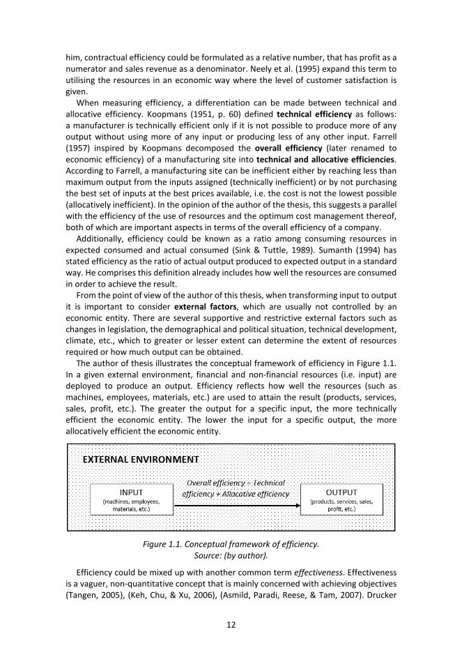
The author of thesis illustrates the conceptual framework of efficiency in Figure 1.1. In a given external environment, financial and non-financial resources (i.e. input) are deployed to produce an output. Efficiency reflects how well the resources (such as machines, employees, materials, etc.) are used to attain the result (products, services, sales, profit, etc.). The greater the output for a specific input, the more technically efficient the economic entity. The lower the input for a specific output, the more allocatively efficient the economic entity.

Figure 1.1. Conceptual framework of efficiency. Source: (by author).

Efficiency could be mixed up with another common term effectiveness. Effectiveness is a vaguer, non-quantitative concept that is mainly concerned with achieving objectives (Tangen, 2005), (Keh, Chu, & Xu, 2006), (Asmild, Paradi, Reese, & Tam, 2007). Drucker

13

(1963) refers to effectiveness as “doing the right things”. According to Fullard (2007), the effectiveness of a company’s services can be assessed based on customer satisfaction. Goh (2013) illustrates the differences between efficiency and effectiveness with the 2х2 grid (Figure 1.2). To reach the top right box, the companies need to be efficient and focused on precise goals in their daily operations.

Figure 1.2. Efficiency and effectiveness. Source: (Goh, 2013).

Mandl, Dierx and Ilzkovitz (2008) speculated when analysing public spending that it is not always easy to isolate efficiency and effectiveness. According to Roghanian, Rasli and Gheysari (2012), several authors compile efficiency (output/input) and effectiveness (goals/input) as productivity. The author of the thesis is of the opinion that effectiveness is a prerequisite to improving overall efficiency, as a company will achieve higher output with fewer resources by combining efficiency and effectiveness.

Nowadays, there are numerous methods of efficiency evaluation. These approaches consist of ratio analysis, manufacturing analysis, data envelopment analysis (DEA), balanced scorecard (BSC), analytic hierarchy process (AHP), fuzzy multiple criteria decision making (MCDM) and more. The following subchapters give an overview of the pioneering and most-cited works in efficiency assessment. At first, the author of the doctoral thesis will focus on different methodologies used in efficiency analysis in the last 90 years in English scientific literature (see subchapter 1.1.2). As the matrix concept studied in this doctoral thesis mainly utilises ratio analysis, broader exploration will be performed on the usage of ratio analysis in previous studies (see subchapter 1.2).

1.1.2 Overview of methodologies used in efficiency analysis In the last century, several methodologies were developed to measure the efficiency of the business activities of companies using both parametric (i.e. functional form is pre-established or determined a priori) and non-parametric techniques (i.e no functional form is pre-defined but is calculated based on the sample observations in an empirical way). In this subchapter an overview of the pioneering works of different methodologies will be given.

14

The author of this doctoral thesis is of the opinion that one of the first attempts to measure efficiency and the changes therein was performed by Cobb and Douglas (1928). They published production function with the aim of a) defining what relationships exist between the three factors of product, capital and labour and b) measuring the changes in the amount of capital and labour that are used to deliver this volume of goods. The production function was extended with duality concepts: Shephard (1953) introduced the cost and production function. McFadden (1972) generalised the duality concepts in production theory and introduced profit and revenue functions. Lau (1972) focused on the properties of profit functions with multiple outputs and inputs. Production, revenue, cost and profit functions could be composed and manufacturing efficiency calculated using the internal financial and non-financial information of the company.

Debreu (1951) sought numerical evaluation of the “dead loss” associated with the non-optimal situation of the economic system and introduced the coefficient of resource utilisation. According to Debreu, “dead loss” could originate from a) underemployed physical resources (labour, machinery, land, etc.), b) inefficiency in the manufacturing process and c) imperfection in the economic system (driven by taxation, monopolies etc.).

Moorsten’s (1961) paper was pioneering on measuring the relative efficiency of production. Moorsten suggested comparing the input of a company in two different points in time with the maximum factor by which the input in one period could be deflated to the level that the company could still produce the output observed in the other time period. This resulted in the so-called Malmquist input index, inspired by the quantity index model proposed by Sten Malmquist (1953) for consumption analysis. A similar Malmquist output index is also available. Neither Malmquist nor Moorsten allowed for any differences over time in the process of manufacturing. Caves et al. (1982) elaborated on the Malmquist deflation idea in the assumption of unrestricted structures of manufacturing during two periods. Malmquist productivity indices could be decomposed to two component measures – technical change and efficiency change as demonstrated by Färe et al. (1994).

As the previous models sacrificed the analysis of random shocks, Meeusen and van den Broeck (1977), Aigner, Lovell and Schmidt (1977), and Battese and Corra (1977) concurrently developed a stochastic frontier model that besides efficiency analysis also captures the effects of external shocks beyond the control of the companies.

The concept introduced by Farrell (1957) led to the development of non-parametric data envelopment analysis (DEA) by Charnes et al. (1978). It is important to note that DEA provides no statistical information on the reliability and goodness of the results as neither any specific statistical distribution of the error terms nor specific functional relationship between manufacturing inputs and outputs is anticipated. However, its ability to engage manufacturing processes involving multiple inputs and multiple outputs makes it an interesting choice and outweighs its statistical deficiencies. However, it is important to bear in mind that according to Kneip, Park and Simar (1998) and Park, Simar and Weiner (2000) the results of DEA may be misleading when small samples are used. DEA obtains detailed information on the relative performance of each decision-making unit (DMU) through an efficiency score (equal to one for efficient DMUs and less than one for inefficient DMUs). For inefficient DMUs, DEA is able to identify its peers from a set of efficient units, as well as improvements in the input and/or output levels required by the unit to become the efficient frontier. Initially, DEA was built to assess the relative efficiency among non-profit organisations (Charnes, Cooper, & Rhodes, 1981).

15

The original DEA-model developed by Charnes et al. in 1978 had a precondition of constant return on scale. Banker et al. (1984) introduced the DEA-model for variable return on a scale where a shift in the input leads to a disproportional transformation in the output. The use of the constant and variable return scale models jointly supports specification of the overall scale and technical efficiencies of the company, as well as whether the data reveals any varying returns to scale or not (Sarkis, 2000). Two-stage DEA-models have been in use since the end of the 1990s. In that case, two successive DEA frontiers are constructed: an output variable of the first frontier will be applied as an input variable into the second frontier. Nowadays, DEA is one of the widespread non-parametric efficiency measurement techniques. There are thousands of peer-reviewed papers using DEA when assessing the relative efficiency of various organisations (Emrouznejad, Parker, & Tavares, 2008).

Van den Broeck et al. (1994) first introduced the usage of Bayesian techniques in an efficiency assessment context to evaluate company-specific efficiencies. Koop, Osiewalski and Steel (1997) applied Bayesian techniques for economic efficiency appraisal on a panel data framework and developed models to analyse inefficiencies at company level by taking into account a company’s specific characteristics. Koop, Osiewalski and Steel (1999) subsequently used Bayesian methods to decompose change in output into technical, efficiency and input changes. Fernandez, Koop and Steel (2000) and (2002) broadened the Bayesian methodology to measure efficiency relative to this technology (how to distinguish between environmental and technical efficiency) and in cases where some of the outputs might be undesirable.

Since the 1990s, there have been many comparative studies published (e.g. Ferrier & Lovell (1990), Bjurek, Hjalmarsson & Forsund (1990), Førsund (1992), Cummins & Zi (1998), Chakraborty, Biswas, & Lewis (2001), Murillo-Zamorano & Vega-Cervera (2001)) in which two or more methods have been used to analyse economic efficiency. Several authors concluded that the choice of method used for the efficiency analysis could make a meaningful effect on the conclusions of an efficiency study.

Kaplan and Norton (1996) created a balanced scorecard (BSC) to link the financial evaluation with customer satisfaction, internal business procedure, innovation and learning ability to help the improvement of product, procedure, customer and market expansion.

Shaverdi et al. (2011) proposed the fuzzy multiple criteria decision making (MCDM) method combined with the BSC approach for assessing performance for three non-governmental Iranian banks. Moreover, fuzzy analytic hierarchy process (FAHP) calculated the relative weights of each chosen index in order to tolerate vagueness and the ambiguity of information, and three MCDM analytical tools (TOPSIS, VIKOR and ELECTRE) were adopted to rank the banking performance.

Shaverdi, et al. (2016) used the fuzzy analytical hierarchy process (AHP) and fuzzy technique for order performance by similarity to ideal solution (TOPSIS) methods to rank companies based on financial performance and concluded that both methods gave similar rankings based on seven Iranian petrochemical companies. Both methods assume the hierarchical financial performance evaluation model is structured using main financial ratios and fuzzy analytic process to determine the weights for each ratio. The opinions of experts were incorporated for the evaluation model in addition to a literature review.

A large amount of applied research has dealt with the measurement of economic efficiency using either parametric or non-parametric techniques or two-step evaluation

16

combining both types of methods. Pursuant to Murillo-Zamorano’s overview (2004) these techniques have been already utilised in a broad range of fields in economics (incl. finance, banking, agriculture, environmental economics, development economics, etc.).

As suggested in this subchapter, a complicated phenomenon such as economic efficiency may be represented by means of an unlimited number of models. Several authors have divided efficiency into factors (components), so that it is easier to analyse the formation of efficiency and change therein. From this, it may be concluded that it is impossible to arrive at a single correct model. In this doctoral thesis, an additional analytical method for the evaluation of the level of efficiency of an economic entity and of change therein by using the principles of complex and system integrated analyses is provided.

1.2 Ascertainment of the most important financial ratios As financial ratios (qualitative indicators) make up an important part of an efficiency matrix, the objective of the next subchapter is to investigate the most common ratios and the limitations of using financial ratios. The use of the most common ratios in an efficiency matrix facilitates understanding of the information in efficiency matrices.

Ratios derived from financial statements are extensively used by both researchers and practitioners for several purposes. These include the evaluation of business and managerial success, prediction of bankruptcy, relationships between financial data and stock exchange characteristics, various industry analyses, etc.

The major reasons for using financial ratios can be summarised as follows (based on (Whittington, 1980) and (Barnes, The analysis and use of financial ratios: a review article, 1987)):

1) to controll the effect of size on financial variables,2) for comparison purposes in evaluating a company’s financial ratios with

industry-wide (average) ratios and other standards,3) for forecasting purposes:

− in statistical models for predicting objectives (e.g. for corporate failure, credit rating, risk assessment, etc.),

− to anticipate future financial variables (e.g. estimation of future gross profit by multiplying forecasted sales by gross margin (gross profit to sales ratio)).

There are two major restrictive assumptions to bear in mind when using ratios for financial statement analysis:

1) proportionality assumption,2) assumption of distributional properties of financial ratios.

1.2.1 Classification of financial ratios

Due to the broad range of different types of users exploiting financial statement analysis, it is obvious that the number of financial ratios used in practice is also large. Therefore, the decision makers first need to classify the large number of ratios into groups and then choose one appropriate ratio from each group to represent a particular aspect of the company. In this context, there are naturally two major problems. First, which groups of financial groups are relevant and second, which ratio(s) describe these dimensions in an appropriate manner. The first annual reports that were certified by public auditors were

17

published in the 1900s. The discussions about determining the most efficacious group of ratios started in literature in the 1920s. Based on the methodology used, the classifications can be divided into empirical, deductive and inductive approaches. Below is an explanation of every classification base separately, citing, in addition, examples from both the most cited and the most recent research papers.

1.2.1.1 Empirical classification A number of financial ratios were created by analysts in the early decades of the 20th century. Two paths of development of ratio analysis were distinguished (Horrigan, A short history of financial ratio analysis, 1968):

1) credit analysis to measure the borrower’s ability to repay loans,2) managerial analysis where profitability measurement was emphasised.

Hardy and Meech (1925) sought an effective set of ratios to be used when performing comparative financial statement analysis and divided ratios into four categories:

1) working capital ratios (e.g. current assets to current liabilities),2) fixed and intangible assets usage ratios (e.g. sales to fixed assets),3) capitalisation ratios (e.g. owners’ equity to liabilities),4) income and expense ratios (e.g. operating profit to sales).

Hardy and Meech emphasised that each ratio has to be expressed in such a way that increases from period to period are favourable and decreases unfavourable to the financial condition.

One of the interesting early papers on financial ratios in which many empirical issues are first discussed is “Some Empirical Bases of Financial Ratio analysis” by James O. Horrigan (1965). Horrigan reviewed a large number of sources related to financial statement analysis and decided to group ratios into liquidity and profitability ratios. He broke the liquidity category down into short-term liquidity and long-term solvency divisions, and he classified profitability category further in line with Du Pont’s return on investment triangulation as follows: assets turnover, profit margin and return on investment. Based on studies from the 1920s to the start of the 1960s, Horrigan created a basic list of financial ratios:

1) Short-term liquidity ratios− Current assets to Current liabilities (“Current ratio”), − Current assets less inventories to Current liabilities (“Quick ratio”), − Cash plus marketable securities to Current liabilities.

2) Long-term solvency ratios− Operating profit to Interest expense (“Times-interest-earned ratio”), − Owners’ equity to Total liabilities, − Owners’ equity to Long-term liabilities, − Owners’ equity to Fixed assets.

3) Turnover ratios− Sales to Accounts receivable, − Sales to Inventories, − Sales to Working capital, − Sales to Fixed assets, − Sales to Net worth, − Sales to Total assets.

4) Profit margin ratios

18

− Operating profit to Sales, − Net profit to Sales.

5) Return on Investment ratios− Operating profit to Total assets, − Net profit to Owners’ equity.

The majority of ratios listed by Horrigan are still in use. However, the author of this doctoral thesis is of the opinion that for long-term solvency ratios the numerator and denominator have to be exchanged. This allows users to easily understand how much liabilities have been attracted in addition to owners’ equity and the proportion of assets, financed by owners’ equity.

One of the traditional and most popular classification patterns presented by Lev (1974, p. 12) categorises financial ratios into four categories:

1) profitability ratios,2) liquidity ratios,3) financial leverage (long-term solvency) ratios,4) efficiency (turnover or activity) ratios.

Kanto and Martikainen (1992) concluded that conventional conceptual interpretation has been used for traditional empirical classifications aiming to illustrate the key dimensions of the company. The categories are oriented according to the needs of different groups of users. For managerial purposes, the profitability and turnover ratios are constructed to evaluate either companies’ operational performance or efficiency. For creditors (suppliers, banks etc.), liquidity and solvency ratios are useful to measure the ability of companies to meet their short-term and long-term financial obligations.

Chen and Shimerda (1981) came to the conclusion that ratios have often been attracted to the models on the basis of their popularity in literature together with a few new ones initiated by the researcher.

According to Zheng and Alver (2015), in 2006 China’s State-owned Assets Supervision and Administration Commission released a financial performance model to assess the operations of state-owned companies in China. There were eight ratios used in the basic model and 14 ratios in the modified model, which were split into four categories:

1) profitability ratios,2) assets quality (i.e turnover) ratios,3) the debt risk profile (i.e. solvency) ratios,4) business growth ratios.

Nowadays empirical classification can be found from many finance and accounting textbooks where subjective classifications of ratios are presented. As the categories are created according to the authors’ specific experiences, it is common that the ratios and classifications in the categories differ among authors. Usually, profitability and liquidity ratios are presented but beyond that there is no clear consensus in the books.

1.2.1.2 Deductive classification Technical (mathematical) relationships are used when classifying ratios in the deductive approach. One of the best-known examples of the deductive approach is the Du Pont triangle system published in 1919 (Salmi & Martikainen, 1994). DuPont explosives salesman Donaldson Brown invented this formula in an internal efficiency report in 1912 (Phillips, 2015). The initial model developed by DuPont for its own use is now used by many companies to evaluate the profitability of assets (return on assets (ROA) ratio). It measures the combined effects of asset turnover and net profit margin:

19

𝑅𝑅𝑅𝑅𝑅𝑅 = 𝑁𝑁𝑁𝑁𝑁𝑁 𝑝𝑝𝑝𝑝𝑝𝑝𝑝𝑝𝑝𝑝𝑁𝑁𝑇𝑇𝑝𝑝𝑁𝑁𝑇𝑇𝑇𝑇 𝑇𝑇𝑎𝑎𝑎𝑎𝑁𝑁𝑁𝑁𝑎𝑎

= 𝑁𝑁𝑁𝑁𝑁𝑁 𝑎𝑎𝑇𝑇𝑇𝑇𝑁𝑁𝑎𝑎𝑇𝑇𝑝𝑝𝑁𝑁𝑇𝑇𝑇𝑇 𝑇𝑇𝑎𝑎𝑎𝑎𝑁𝑁𝑁𝑁𝑎𝑎

× 𝑁𝑁𝑁𝑁𝑁𝑁 𝑝𝑝𝑝𝑝𝑝𝑝𝑝𝑝𝑝𝑝𝑁𝑁𝑁𝑁𝑁𝑁𝑁𝑁 𝑎𝑎𝑇𝑇𝑇𝑇𝑁𝑁𝑎𝑎

(1.1)

Nowadays, three components (financial leverage, assets turnover and profit margin) are often used to compute return of equity (ROE)1 by parts:

𝑅𝑅𝑅𝑅𝑅𝑅 = 𝑁𝑁𝑁𝑁𝑁𝑁 𝑝𝑝𝑝𝑝𝑝𝑝𝑝𝑝𝑝𝑝𝑁𝑁𝐴𝐴𝐴𝐴𝑁𝑁𝑝𝑝𝑇𝑇𝐴𝐴𝑁𝑁 𝐸𝐸𝐸𝐸𝐸𝐸𝑝𝑝𝑁𝑁𝐸𝐸

= 𝐴𝐴𝐴𝐴𝑁𝑁𝑝𝑝𝑇𝑇𝐴𝐴𝑁𝑁 𝐴𝐴𝑎𝑎𝑎𝑎𝑁𝑁𝑁𝑁𝑎𝑎𝐴𝐴𝐴𝐴𝑁𝑁𝑝𝑝𝑇𝑇𝐴𝐴𝑁𝑁 𝐸𝐸𝐸𝐸𝐸𝐸𝑝𝑝𝑁𝑁𝐸𝐸

× 𝑁𝑁𝑁𝑁𝑁𝑁 𝑎𝑎𝑇𝑇𝑇𝑇𝑁𝑁𝑎𝑎𝐴𝐴𝐴𝐴𝑁𝑁𝑝𝑝𝑇𝑇𝐴𝐴𝑁𝑁 𝐴𝐴𝑎𝑎𝑎𝑎𝑁𝑁𝑁𝑁𝑎𝑎

× 𝑁𝑁𝑁𝑁𝑁𝑁 𝑝𝑝𝑝𝑝𝑝𝑝𝑝𝑝𝑝𝑝𝑁𝑁𝑁𝑁𝑁𝑁𝑁𝑁 𝑎𝑎𝑇𝑇𝑇𝑇𝑁𝑁𝑎𝑎

(1.2)

The three-component model enables the analyst to understand the sources of ROE when comparing different companies or industries. In general, all industries can be split into high margin industries (e.g. manufacturing industries), high turnover industries (e.g. retail and service industries) and high leverage industries (e.g. financial sector).

The Du Pont formula could be split further. Bodie et al. (2004, pp. 458–459) propose to decompose ROE into five components:

𝑅𝑅𝑅𝑅𝑅𝑅 = 𝑁𝑁𝑁𝑁𝑁𝑁 𝑝𝑝𝑝𝑝𝑝𝑝𝑝𝑝𝑝𝑝𝑁𝑁𝐴𝐴𝐴𝐴𝑁𝑁𝑝𝑝𝑇𝑇𝐴𝐴𝑁𝑁 𝐸𝐸𝐸𝐸𝐸𝐸𝑝𝑝𝑁𝑁𝐸𝐸

= 𝐴𝐴𝐴𝐴𝑁𝑁𝑝𝑝𝑇𝑇𝐴𝐴𝑁𝑁 𝐴𝐴𝑎𝑎𝑎𝑎𝑁𝑁𝑁𝑁𝑎𝑎𝐴𝐴𝐴𝐴𝑁𝑁𝑝𝑝𝑇𝑇𝐴𝐴𝑁𝑁 𝐸𝐸𝐸𝐸𝐸𝐸𝑝𝑝𝑁𝑁𝐸𝐸

× 𝑁𝑁𝑁𝑁𝑁𝑁 𝑎𝑎𝑇𝑇𝑇𝑇𝑁𝑁𝑎𝑎𝐴𝐴𝐴𝐴𝑁𝑁𝑝𝑝𝑇𝑇𝐴𝐴𝑁𝑁 𝐴𝐴𝑎𝑎𝑎𝑎𝑁𝑁𝑁𝑁𝑎𝑎

× 𝐸𝐸𝐸𝐸𝐸𝐸𝑇𝑇𝑁𝑁𝑁𝑁𝑁𝑁 𝑎𝑎𝑇𝑇𝑇𝑇𝑁𝑁𝑎𝑎

× 𝐸𝐸𝐸𝐸𝑇𝑇𝐸𝐸𝐸𝐸𝐸𝐸𝑇𝑇

× 𝑁𝑁𝑁𝑁𝑁𝑁 𝑝𝑝𝑝𝑝𝑝𝑝𝑝𝑝𝑝𝑝𝑁𝑁𝐸𝐸𝐸𝐸𝑇𝑇

(1.3)

In the case of DuPont’s model, a parallel may be drawn to an efficiency matrix whose elements are interlinked. Thus, using the chain-linking method, change in the net profit margin of owners’ equity may also be analysed by component by determining the absolute impact of change in every component on change in the net profit margin of owners’ equity.

Based on earlier studies and textbooks, Courtis (1978) created a diagram where the visual approximation of relations between 79 ratios was presented. Courtis classified these 79 ratios into three categories (Figure 1.3):

1) Profitability ratios indicating if there has been a satisfactory rate of returnfrom business activities.

2) Managerial performance ratios to be used to investigate specificmanagement functions: credit policy, inventory, administration and assets-equity structure. Credit policy and inventory ratios indicate movements incurrent assets and seek to assess the effectiveness of credit management and the efficiency of the company’s inventory management. The administrationratios (operating expenses/sales, operating expenses/total assets) areintended to measure the effectiveness of cost control and have a clear linkwith the profitability category above. Courtis positioned the asset-equitystructure category under management performance category (instead ofsolvency category) to emphasise the importance of appraising under/overcapitalisation, the relative proportions of current and fixed assets and theextent to which long-term assets are being financed by long-term liabilities.

3) Solvency ratios can be subdivided into short-term liquidity, long-termsolvency and cash flow ratios. Short-term liquidity ratios (currentassets/current liabilities, current assets/sales, current liabilities/net worthetc.) indicate “technical” solvency to pay all current liabilities. Long-termsolvency ratios (total liabilities/net worth, total liabilities/total assets,EBIT/interest expense etc.) assess the capability to pay both long-termliabilities and related interests. Cash flow sub-category ratios (cash flow/total

1 Traditionally the end of the fiscal year balance sheet data is used in the Du Pont formula. The author of the thesis prefers average values of balance sheet indicators to ensure better comparability with income statement information.

20

liabilities, cash flow/current liabilities, cash flow/sales etc.) consider liquidity through the maintenance of adequately matched periodic cash inflows and outflows.

As traditional financial analysis models were developed in an age when cash flow data were not available, Courtis separately grouping ratios including cash flow information indicates a new era in financial statement analysis. However, in his paper Courtis only used the term “cash flow” in the formulas and did not specify which type of cash flow (either operating, investing, free or financing) had to be included when calculating ratios.

Figure 1.3. Financial ratios categorical framework. Source: (Courtis, 1978).

The UK based Centre of Intercompany Comparisons (CIFC) tested the statistical significance differences between the average values of the ratios of inner city and other locations. The main conclusion of the study is that manufacturing profitability is lower in the inner cities (Fothergill, Kitson, & Monk, 1982). They concentrated a 'pyramid' approach consisting of an assets profitability ratio on the top that is definitionally related to further 'constituent' ratios lower down (Figure 1.4).

Carlino, et al. (2017) researched the decomposition of differences in three aggregate financial ratios (Equity to Assets, Financial liabilities to Assets, EBIT to Sales) of approximately 1,000 European non-financial listed companies using Laspeyres-index based methodology. They analysed differences in the ratios in two dimensions: 1) cross-country comparison at a given point of time across eight countries and 2) temporal decomposition at two points of time. In both cases, differences at sectoral ratios were decomposed into differences in structure as well as differences in sectoral ratios.

21

Figure 1.4. An example of “Pyramid of ratios” approach. Source: (Fothergill, Kitson, & Monk, 1982).

In general, the deductive approach seeks to explain differences in the higher ratios by identifying further differences in the lower ones. Nowadays, the deductive approach has become mixed with a concompanyatory approach, which will be discussed later.

1.2.1.3 Inductive classification Statistical techniques are used to classify financial ratios in the inductive approach. The aim is to reduce the large number of ratios to a smaller number of mutually exclusive categories covering different aspects of companies’ activities. Empirical foundations rather than theoretical foundations for grouping ratios are characteristic of the inductive approach (Salmi & Martikainen, 1994).

Multiple discriminant analysis (MDA) is well suited to many finance problems where the dependent variable is nonmetric (efficient or non-efficient, bankrupt or not bankrupt, etc.). MDA is using ratio data to develop a linear model that best discriminates between different groups of companies. The primary objective of MDA is to classify entities correctly into mutually exclusive groups by the statistical decision rule of maximising the ratio of among-groups to within-groups variance-covariance from the set of independent variables. In addition, MDA reveals which of the variables has contributed the most to group discrimination. MDA is further suited to finance applications because, as a multivariate technique, it treats a profile of variables, rather than one variable at a time.

The best-known discriminant functions are related to companies’ bankruptcy predictions. For example, Altman (1968) used MDA to generate a Z-score model including a combination of variables that best discriminated between failed and non-failed companies. Altman evaluated a list of 22 potentially helpful ratios. The ratios were classified into five standard ratio categories, including profitability, leverage, liquidity, solvency and activity ratios. The ratios were chosen on the basis of their popularity in existing literature and potential relevancy to his study. From the original list of variables, five variables (Working Capital/Total Assets, Retained Earnings/Total Assets, EBIT

22

(Earnings before interests and taxes)/Total assets, Market value of equity/Total liabilities and Sales/Total assets) were finally selected as performing the best overall job together. Chakavarthy (1986) speculated that even Z-scores are mainly built to predict business failure; the distance from Z-value could also be used as the overall indicator of well-being of the company. Owners often emphasise that profitability is the most important measure for the company, though it may happen that a profitable company cannot be considered efficient due to a shortcoming in its usage of resources. Chakavarthy included eight weakly correlated ratios (operating cash flow to investment cash flow, sales to total assets, R&D expenses to sales, market value to book value, sales per employee, liabilities to equity ratio, working capital to sales ratio and dividend payout ratio) to the discriminant function of his study. He concluded that this discriminant function distinguished efficient companies in 73% of the sample.

In most empirical studies in finance, the multicollinearity problem occurs when using MDA with ratios. An assumption of most statistical techniques derived from the general linear model is that the independent variables are mutually uncorrelated. Although moderate exceptions from this do not significantly impair the results, when the variables are highly collinear, the weights in the resulting model are highly unstable, the model tends to be highly sample sensitive and interpretation becomes very difficult. Discriminant analysis is not the only option for the construction of ratio models (e.g. failure-prediction). Other possible techniques include the linear probability model, logit analysis and probit analysis. Although, as presented by Killough, Koh and Tsui (1989), the prediction accuracy rates of failure-prediction models constructed with different statistical classification techniques do not differ significantly, and none of the techniques is consistently superior to other techniques. Thus, discriminant analysis has often been selected because it is relatively easy to understand and apply, and it is more readily available when compared with logit or probit analysis.

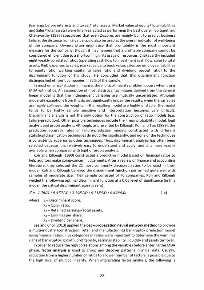
Koh and Killough (1990) constructed a predictive model based on financial ratios to help auditors make going-concern judgements. After a review of finance and accounting literature, they selected the 21 most commonly discussed ratios to be used in their model. Koh and Killough believed the discriminant function performed quite well with samples of moderate size. Their sample consisted of 70 companies. Koh and Killough yielded the following optimal discriminant function at a 0.05 level of significance (in this model, the critical discriminant score is zero):

Z =–1.2601+0.8701X1+2.1981X2+0.1184X3+0.8960X4, (1.4)

where Z – Discriminant score, X1 – Quick ratio, X2 – Retained earnings/Total assets, X3 – Earnings per share, X4 – Dividend per share.

Lee and Choi (2013) applied the back-propagation neural network method to provide a multi-industry (construction, retail and manufacturing) bankruptcy prediction model using financial ratios. Five categories of ratios were important to determine the warnings signs of bankruptcy: growth, profitability, earnings stability, liquidity and assets turnover.

In order to reduce the high correlations among the variables before entering the MDA phase, factor analysis is used to group and discover patterns in initial data. Usually, reduction from a higher number of ratios to a lower number of factors is possible due to the high level of multicollinearity. When interpreting factor analysis, the following is

23

generally considered: (a) the number of distinct factors, (b) how the original data are grouped in the factors, and (c) if the factors can be given a meaningful interpretation in terms of the research problem. These factor patterns have the property of retaining the maximum amount of information (i.e. explaining the maximum variance) contained in the original data. Factor analysis can be used to isolate the independent patterns of financial ratios.

One of the first attempts at financial ratio classifications using factor analysis was performed by Pinches, Mingo and Caruthers (1973) based on the financial ratios of 221 industrial companies. In addition to ratio classifications, the purpose of their study was to measure long-term stability in these classifications over the period of 1951–1969. Johnson (1979) continued the Pinches et al. research and concompanyed the financial ratio patterns already identified by performing principal component analysis of the 61 ratios for 306 primary manufacturing and 159 retailing companies in 1972 and 1974. Either Pinches et al. or Johnson selected factor loading 0.70 because it implies that the financial ratios account for approximately 50% of the factor’s variance. Variables with less than 50% common variation with factor pattern were considered too weak to report.

Pinches et al. and Johnson agreed on seven factors: 1) Return on investment (18 ratios, including sales and assets profitability ratios

as well cash flow ratios),2) Capital turnover (16 ratios, mainly including assets turnover ratios),3) Inventory turnover (8 ratios, mainly including inventory and working capital

ratios),4) Financial leverage (13 ratios, mainly including liabilities related ratios),5) Receivables turnover (7–8 ratios2, mostly including quick assets and

receivable ratios),6) Short-term liquidity (8 ratios, mostly including current liabilities related

ratios),7) Cash position (4–5 ratios, mainly comparing cash to other asset groups).

Johnson also added an eighth dimension: Growth ratios (measures the current year relative to a former one for asset items as well as sales). Pinches et al. (1973) concluded that the composition of these groups is reasonably stable over time, even when the magnitude of the financial ratios are undergoing change. From this author’s point of view, both authors faced challenges in grouping sales profitability and inventory turnover ratios, as sales profitability ratios can be found in factor 1 and factor 2 and inventory turnover ratios in factor 3 and factor 5.

Laurent (1979) identified a small set of financial ratios through factor analysis which 1) account for proportion of the total variance in a relatively complete set of financialratios, 2) are sufficiently few in number to increase the efficiency and effectiveness of financial ratio analysis and 3) are sufficiently independent of each other to permit proper identification of their individual effects in multivariate analysis. The financial ratios Laurent selected to represent each factor are listed in Table 1.1.

Chen and Shimerda (1981) demonstrated that the financial ratios investigated in the previous predictive studies of bankruptcy could be classified into five factors (return on investment, capital turnover, financial leverage, cash position, receivables turnover). Because the ratios classified within the same factor have a high correlation, they

2 Quick Assets to Capital Expenditures ratio was included in factor 5 by Johnson and factor 7 by Pinches et al.

24

suggested selecting one ratio that accounts for most of the information to represent a particular factor. The inclusion of more than one ratio from a factor leads to multicollinearity among ratios and distorts the relationship between independent and dependent variables.

Table 1.1. Financial ratios selected to represent each factor.

Factor Financial ratio Return on investment EBIT to Assets Gearing Long-term liabilities to Assets Working capital management Sales to Working capital Fixed asset management Sales to Fixed assets Long-term solvency Sales to Equity Short-term solvency Current assets to Current liabilities Inventory management Sales to Inventory Standing changes cover (liquidity to long-term liabilities)

EBIT to Interest expense

Income retention policy Reserves to Net profit Credit policy Sales to Account Receivable

Source: (Laurent, 1979).

Cowen and Hoffer (1982) concluded that consistent and logical ratio groupings may not exist at single industry level; however, different sets of ratios tend to move together.

Gombola and Ketz (1983a) performed factor analysis based on 58 financial ratios from 119 industrial companies and identified cash flow measures as a separate dimension of company performance.

Hutchinson, Meric and Meric (1988) presented six principal components for 127 small companies, which were quoted on the UK Unlisted Securities market. For each component, the ratio with the highest factor loadings was published (Table 1.2).

Table 1.2. Principle components and the financial ratios representing the best every component.

Principle component (factor) Ratio Indebtedness and Liquidity Equity to Total assets Profitability Earnings before interest and tax to Total

assets Growth rate Annual average sales growth rate (two year

average for the period t–5 and t–3) Assets structure Current assets to Total assets Assets turnover Sales to Total Assets Accounts receivable level Accounts receivable to Sales

Source: (Hutchinson, Meric, & Meric, 1988).

Yli-Olli and Virtanen (1985) modelled financial ratio classification at economy-wide level. They selected 12 financial ratios to be classified and measured the long-term stability of these ratios. The sample varied from 450 companies in 1947 to 1,500 companies in 1975. The data only included financial information from industrial companies closing the financial year at the end of December. As per Yli-Olli and Virtanen,

25

the use of companies with a similar fiscal year gives a clearer picture of the different phases of economic cycles than the use of all companies regardless of their financial year. Yli-Olli and Virtanen used factor and transformation analysis and found the following factors (10 ratios out of 12 were classified):

1) Solvency (Liabilities to Equity, Quick ratio),2) Profitability (ROE, ROA, Net profit margin, Times interest earned),3) Efficiency (Assets turnover, Inventory turnover, Accounts receivable

turnover),4) Dynamic liquidity (Defensive interval measure).

One highly interesting piece of research in the author’s view is the paper by Salmi, Virtanen and Yli-Olli (1990) where they introduced three main categories of ratios: accrual ratios, cash flow ratios and market-based ratios. Before, there had been little research involving cash flow ratios and Salmi et al. were the first to investigate market-based ratios. They used factor analysis and transformation analysis. The latter method was used to test the temporal stability of the financial ratio factors. Six stable factors of financial ratio information were identified by factor and transformation analyses based on the data of 32 publicly traded Finnish companies in 1974–1984. The stable factors were profitability, operational leverage, cash flow, size & beta, liquidity and growth rate factors. The authors made the following conclusions:

1) Cash flow ratios were loading on a separate and distinct stable factor. Thisconcompanyed earlier results that cash flow ratios impart information notpresented in the accrual-based financial ratios.

2) Market-based ratios dispersed widely on different factors; the authorsproposed that unlike accrual and cash flow financial ratios, market-basedratios simply are not amenable to a consistent categorisation.

3) The results did not directly support the conventional classification (i.e. thestandard textbook financial ratio classification into profitability, liquidity,solvency, and turnover) of ratios.

Luoma and Ruuhela (1991) applied cluster analysis to a group of five pre-defined financial ratio categories (profitability, financial leverage, liquidity, working capital and cash flow ratios) including 15 financial ratios based on the financial data of 40 Finnish companies in 1974–1984. They chose cluster analysis instead of the commonly used factor analysis because criterions for determining factors may often give too many factors and some of them might be artificial. Contrary to factor analysis in cluster analysis, ratio can only belong to one cluster. Their results indicate that three categories were enough to encompass the important information of the 15 ratios: profitability, financial leverage and cash flow ratios.

Kanto and Martikainen (1992) introduced concompanyatory factor analysis to test earlier classifications of financial ratios and concluded that selected factors – profitability, financial leverage, liquidity and efficiency – were significantly correlated and are insufficient to illustrate the key dimensions of the companies’ financial performance. Kanto and Martikainen emphasise that the interpretation of factors created should always be carried out with extreme caution. This is required because in most studies factors consist of high loadings representing different a priori financial ratio categories. If the factors cannot be interpreted clearly, the usefulness of these categories in practice is relatively low.

26

Erdogan (2013) conducted factor analysis to reduce nine financial ratios of TOP 500 Turkish industrial companies into a smaller number of factors. Four distinct factors were determined:

1) Productivity (Gross value added to Number of employees and Gross valueadded to Assets),

2) Profitability and Capital structure (EBT margin, ROE, Liabilities to Assets),3) Efficiency (Assets turnover, Equity turnover),4) Export Intensity and Proportion of sales from production.

Delen, Kuzey and Uyar (2013) employed a two-step analysis methodology: first, using exploratory factor analysis to identify underlying dimensions of the financial ratios, followed by using predictive modelling methods to discover the potential relationships between the company performance and financial ratios. Four popular decision tree algorithms (CHAID, C5.0, QUEST and C&RT) were used to investigate the impact of financial ratios on company performance. The result obtained using ROE as the dependent variable indicated that the most important financial ratios were EBT to Equity, Net profit margin, Leverage ratio and Sales growth ratios. These variables had the highest impact on predicting ROE. EBT to Equity was the most important factor in each of the four decision tree models. The findings for the models where ROA was used as the dependent variable indicated that the most important financial ratios were the EBT to Equity, Net profit margin, Debt ratio and Assets turnover ratios.

The main criticism when using statistical techniques can be summarised as follows (Eisenbais (1977), Pinches (1980), Zmijewski (1984) and the opinion of this author):

− the assumptions of multivariate normality in the distribution of the sample groups and the equality of the group dispersion,

− problems in determining the relative importance of individual variables, − reducing the number of variables that do not significantly contribute to the

overall discriminating model, − sample bias (e.g. 'oversampling' failed companies due to the relatively low

frequency rate of company failures, as several studies use a 1:1 ratio in their samples of failed and non-failed companies),

− question of the stability of the model and ratios over time: a model is only useful for predictive purposes if the underlying relationships and indicators are stable over time,

− the results of ratio categorisation based on factor analysis depend significantly on the range of financial ratios included in the factor analysis,

− a disadvantage of factor analysis is ratio may be included in several factors.

The study demonstrated that despite the classification methodology, there is only consensus about the most commonly used ratio categories of profitability and liquidity, but other ratio categories differed across studies. It can also be concluded that factor analysis is mainly used to classify ratios using statistical methods.

The compilation of the efficiency matrix has similarities with deductive classification where technical relationships are used for ratio classification. Additionally, statistical methods (mainly factor analysis) can be used to decide which ratios are the most meaningful in explaining the financial data chosen by the analyst and bearing this in mind when selecting quantitative indicators for the efficiency matrix.

27

1.2.2 Popularity of financial ratios in scientific literature

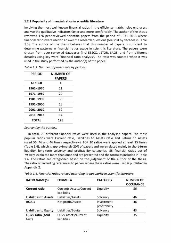
Involving the most well-known financial ratios in the efficiency matrix helps end users analyse the qualitative indicators faster and more comfortably. The author of the thesis reviewed 126 peer-reviewed scientific papers from the period of 1931–2013 where financial ratios were used to answer the research questions (see split by decades in Table 1.3). The author of the thesis believes that this number of papers is sufficient to determine patterns in financial ratios usage in scientific literature. The papers were chosen from peer-reviewed databases (incl EBSCO, JSTOR, SAGE) and from different decades using key word “financial ratio analysis”. The ratio was counted when it was used in the study performed by the author(s) of the paper.

Table 1.3. Number of papers split by periods.

PERIOD NUMBER OF PAPERS

to 1960 4 1961–1970 11 1971–1980 20 1981–1990 30 1991–2000 15 2001–2010 32 2011–2013 14

TOTAL 126

Source: (by the author).

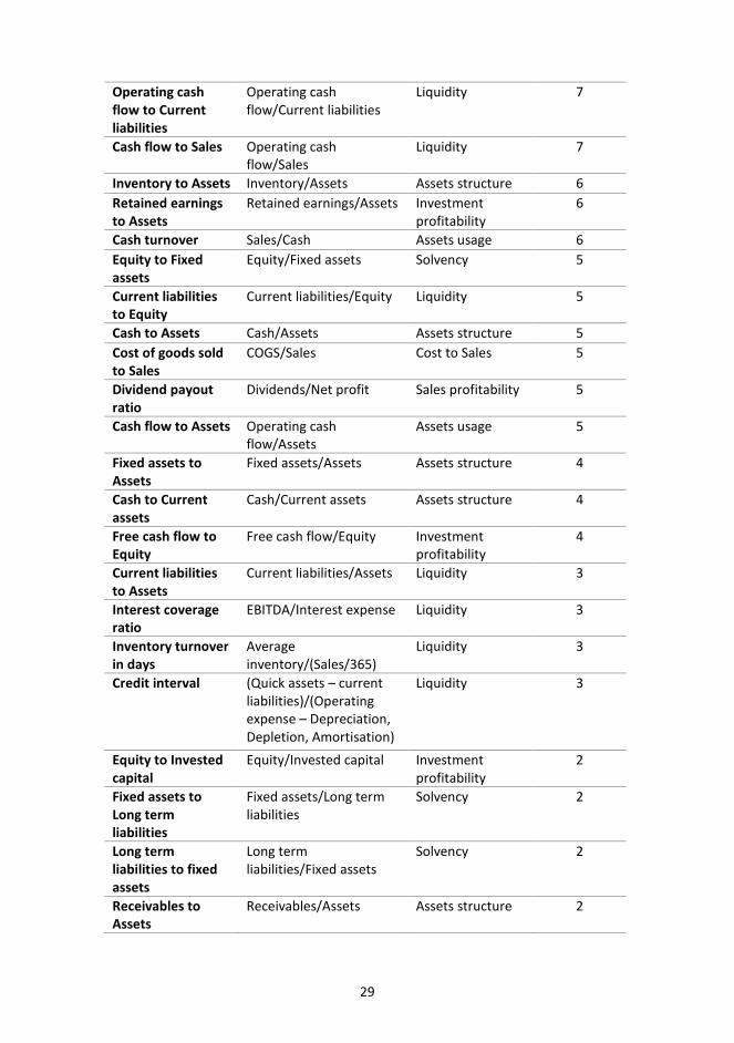
In total, 79 different financial ratios were used in the analysed papers. The most popular ratios were Current ratio, Liabilities to Assets ratio and Return on Assets (used 56, 46 and 46 times respectively). TOP 10 ratios were applied at least 25 times (Table 1.4), which is approximately 20% of papers and were related mainly to short-term liquidity, long-term solvency and profitability categories. 55 financial ratios out of 79 were exploited more than once and are presented and the formulas included in Table 1.4. The ratios are categorised based on the judgement of the author of the thesis. The ratio list including references to papers where these ratios were used is published in Appendix 2.

Table 1.4. Financial ratios ranked according to popularity in scientific literature.

RATIO NAME(S) FORMULA CATEGORY NUMBER OF OCCURANCE

Current ratio Currents Assets/Current liabilities

Liquidity 56

Liabilities to Assets Liabilities/Assets Solvency 46 ROA 1 Net profit/Assets Investment

profitability 46

Liabilities to Equity Liabilities/Equity Solvency 43 Quick ratio (Acid test)

Quick assets/Current liabilities

Liquidity 35

28

Net profit margin Net profit/Sales Sales profitability 33 ROE 1 Net profit/Average

equity Investment profitability

33

Inventory turnover3

Sales/Inventory Assets usage 28

Assets turnover Sales/Assets Assets usage 27 ROA 2 EBIT/Assets Investment

profitability 25

Working capital to Assets

Working capital/Assets Assets usage 23

Operating profit margin

Operating profit/Sales Sales profitability 19

Receivables turnover

Sales/Receivables Assets usage 17

Working capital turnover

Sales/Working Capital Assets usage 15

Current assets turnover

Sales/Currents Assets Assets usage 14

Equity to Assets Equity/Assets Assets structure 12 Current assets to Total assets

Current Assets/Assets Assets structure 12

Times interest earned ratio

EBIT/Interest expense Liquidity 12

Operating cash flow to Total liabilities

Operating cash flow/Liabilities

Liquidity 12

Quick assets to Total assets

Quick assets/Assets Assets structure 10

Cash ratio Cash/Current liabilities Liquidity 10 Profit to liabilities ratio

EBITDA/Liabilities Investment profitability

10

Long term liabilities to Total assets

Non-current liabilities/Assets

Solvency 9

Quick assets turnover

Sales/Quick assets Assets usage 9

ROE 2 Operating profit/Average equity

Investment profitability

8

Long term liabilities to Equity

Non-current liabilities/Equity

Solvency 7

Fixed assets turnover

Sales/Fixed assets Assets usage 7

3 Although Sales is often used when calculating Inventory turnover, it is more appropriate to use Cost of goods sold (COGS) to ensure comparability of numerator and denominator.

29

Operating cash flow to Current liabilities

Operating cash flow/Current liabilities

Liquidity 7

Cash flow to Sales Operating cash flow/Sales

Liquidity 7

Inventory to Assets Inventory/Assets Assets structure 6 Retained earnings to Assets

Retained earnings/Assets Investment profitability

6

Cash turnover Sales/Cash Assets usage 6 Equity to Fixed assets

Equity/Fixed assets Solvency 5

Current liabilities to Equity

Current liabilities/Equity Liquidity 5

Cash to Assets Cash/Assets Assets structure 5 Cost of goods sold to Sales

COGS/Sales Cost to Sales 5

Dividend payout ratio

Dividends/Net profit Sales profitability 5

Cash flow to Assets Operating cash flow/Assets

Assets usage 5

Fixed assets to Assets

Fixed assets/Assets Assets structure 4

Cash to Current assets

Cash/Current assets Assets structure 4

Free cash flow to Equity

Free cash flow/Equity Investment profitability

4

Current liabilities to Assets

Current liabilities/Assets Liquidity 3

Interest coverage ratio

EBITDA/Interest expense Liquidity 3

Inventory turnover in days

Average inventory/(Sales/365)

Liquidity 3

Credit interval (Quick assets – current liabilities)/(Operating expense – Depreciation, Depletion, Amortisation)

Liquidity 3

Equity to Invested capital

Equity/Invested capital Investment profitability

2

Fixed assets to Long term liabilities

Fixed assets/Long term liabilities

Solvency 2

Long term liabilities to fixed assets

Long term liabilities/Fixed assets

Solvency 2

Receivables to Assets

Receivables/Assets Assets structure 2

30

Inventory to Quick assets

Inventory/Quick assets Assets structure 2

Inventory to Current liabilities

Inventory/Current liabilities

Liquidity 2

Return on Fixed Assets

Net profit/Non-current assets

Investment profitability

2

ROA 3 EBITDA/Assets Investment profitability

2

Accounts payable turnover

Accounts payable/(Purchases/365)

Liquidity 2

Labour productivity

Gross value added/Number of employees

Employee usage 2

Source: (by the author).

When summarising ratios by categories (Table 1.5), it can be concluded that short-term liquidity ratios (14 out of 55) were mostly used in the scientific research. This could be explained by the fact that liquidity and the prediction of business failure have been the most interesting and well-researched areas in financial statement analysis. The next four categories consist of 7–10 financial ratios and explain efficiency of assets usage (assets turnover), investment profitability, assets structure and long-term solvency (incl financial leverage). Assets usage and investment profitability ratios should be used when compiling an efficiency matrix based on information from annual reports.

Table 1.5. Number of popular ratios split by categories.

CATEGORY NUMBER OF RATIOS

Liquidity 14 Assets usage 10 Investment profitability 10 Assets structure 9 Solvency 7 Sales profitability 3 Labour usage 1 Cost to Sales 1

Source: (by the author).

Surprisingly to the author, there were many areas of business that affect overall performance and efficiency of the company that are not covered or covered marginally by financial ratios. Sales profitability, efficiency of labour usage, cost efficiency and earnings quality are the main examples of business aspects that are poorly covered by popular financial ratios. This leads to the conclusion that there is a clear need for a tool that supports comprehensive business performance and efficiency analysis.

31

1.2.3 Restrictions of financial ratio usage in financial statement analysis

The use of ratios is based on the assumption of the relationship between the numerator variable (e.g. net profit) and denominator size variable (e.g. total assets). According to Barnes (1987), size is only properly controlled when the two financial variables (x and y, where x is a measure of size) are strictly proportional. That is, y = bx, and the ratio y/x = b. The strict assumption of proportionality is violated if (i) there is an intercept term a, and a≠0, (ii) where there is an error term e; in which cases y = a + bx + e. Clearly in the case of (i), the ratio does not satisfactorily control for size y/x = b + a/x. In the case of (ii), this depends on the behaviour of e. Apparently, whether the use of a specific ratio provides adequate control of size depends on the nature of the relationship, which can be derived from either theoretical or empirical evidence.

To estimate functional relationship properly, it is necessary to estimate intercept and for that regression analysis could be used. There have been several empirical studies since the 1980s (e.g. Lee (1985), Buijink and Jegars (1986) and McLeay and Fieldsend (1987)) that have tested the proportionality assumption. Tippett (1990) concluded that there are relatively few occasions in which the proportionality assumptions can be justified. Sudarsanam and Taffler (1995) selected 24 commonly used ratios with three widely employed denominators: sales, total assets and owners’ equity. The analysis was conducted separately for six distinct industries for a large sample of over 500 companies for two separate years, 1981 and 1986. The Sudarsanam and Taffler results indicated that the relationship between ratio components is, generally, both non-proportionate and non-linear and concluded that loglinearity gives a more valid description of the relationship in the majority of cases examined.

Lev and Sunder (1979) found the following methodological problems related to the use of ratios:

1) Conditions for adequate size control. There are three types of deviationswhen strict proportionality does not hold:

a. the presence of error,b. the presence of an intercept,c. dependence on other variables and non-linearity.

2) Choice of the size variable. Stigler (1968, p. 30) recommends measuring acompany’s size by sales in a product market, by assets in capital market, bycost of goods sold in material market and by employees in a labour market.For example, if the productivity of capital employed is analysed, then netprofit as a function of equity (measured in either book or market value) isappropriate. When employee productivity is of interest, then the total output relative to the number of employees (or to total man-hours) could be ameaningful measure of size.

3) Control of size with negative numbers. For example, a change in a variable(e.g., net profit) that has a ‘positive’ effect on the ratio before the change ofsign will have a ‘negative’ effect after the change of sign. This loss ofcontinuity is a recurring cause of problems in interpreting ratios calculatedfrom negative numbers. Consider, for example, the case where thenumerator of a ratio changes its sign from one period to another, such as thenet profit to equity (or total asset) ratio, where net profit was negative oneyear and positive the following year. In this case, where the company’sprofitability has obviously improved, the relative change of the net profit toequity ratio will be negative (assuming equity is positive). This basic problem

32

renders ratios a risky instrument of controlling for size in the presence of negative numbers, and the investigator should seek alternative means of exercising such control whenever feasible. Lev and Sunder (1979) found that the problems associated with certain negative variables and their ratios could be mitigated by a simple modification of the ratio form. The net profit figure is perceived to be one of the most sensitive of all major financial variables to take negative values. Net profit, Pt, of a company during period t can be treated as the difference between the beginning- and ending-period owners’ equity, respectively Et-1 and Et, after the appropriate adjustments for capital transactions have been made to the ending-period owners’ equity. Adjustments to ending-period owners’ equity include (a) adding the cash dividends declared and share re-purchases, and (b) subtracting new shares issued. Therefore, the ratio Et/Et-1 is equal to the traditional return on equity plus 1, and in general will be positive. This mitigates the problem of discontinuity posed by the companies’ negative net profit.

The usage of financial ratios in statistical models assumes multivariate normality. Data could be forced into a normal distribution when possible. As a result of the distribution analysis of eleven financial ratios Deakin (1976) performed for 454–1,114 manufacturing companies over 19 fiscal years (1955–1973), it appeared that the assumption of normality of ratios is not tenable. Deakin concluded that the normality assumption was improvable in certain cases, while square root and logarithmic transformations were used, but no general guidelines could be given. Frecka and Hopwood (1983) showed that the non-normality of ratios used by Deakin was mainly the result of outliers. Frecka and Hopwood applied square-root transformation to financial ratios, and then identified and removed outliers utilising skewness and kurtosis statistics of the transformed ratios. When using the Chi-square test of normality, almost all of the industry ratios became normally distributed.

Barnes (1982) demonstrated that, because of the relationship between the two variables, financial ratios are likely to be normally distributed in quite unusual situations. As per Barnes, where financial ratios are non-normally distributed, the comparison of a financial ratio with some standard (e.g. the industry average) is likely to misinform. However, he also showed that normality is irrelevant where financial ratios are inputs to certain statistical models (regression analysis and multiple discriminant analysis). Barnes argued that the usual transformation methods such as square roots or natural logarithms as suggested by Deakin (1976) merely confuse the data further.

Cannon (2002) tested several normality remediation methods (incl deletion of outliers) and concluded that the removal of contaminants is the superior method to others when improving normality. Potential sources of contaminants are negative equity, companies facing bankruptcy, companies that have ever made a profit, companies at developmental stage (started less than two years ago) and companies that have undergone a merger within the previous fiscal year.

Thus, it has to be taken into consideration when using financial ratios that empirically there might not be a strictly proportional relationship (y = bx, and the ratio y/x = b) and the minimum that the analyst can do when applying statistical methods (e.g. using factor analysis to determine is the removal of outliers).

33

1.3 Nature of the complex analysis of the economic activities of a company The direction of the complex analysis of economic activities (hereinafter: complex analysis) began to develop in the Soviet Union in the 1950s. The first comprehensive paper was published in 1974 by Professor Anatoli Sheremet (Шеремет, 1974). According to this methodology, the order of the performance of complex analysis and the benchmarks underlying evaluations (standards set and indicators for the budget and previous years) were important. Sheremet divided complex analysis into 13 consecutive phases that are passed through (Figure 1.5).

Figure 1.5. Formation and investigation of main indicator groups in a complex analysis system according to A. Sheremet. Source: (Баканов & Шеремет, 1981, p. 159).

The first and second phases create the basis for the subsequent in-depth analysis of financial indicators. The first phase provides an overview of the main financial indicators of a company and an initial evaluation of these indicators. Whereas at the time of the development of the methodology the main base for the formation of an initial evaluation

34

was comparison to planned-for indicators, today, in addition to comparison to the budget, an overall evaluation may also be formed by comparison to the company’s financial indicators for a previous period, quantiles for its field of activity and indicators for the market leader. The initial evaluation provided in the first phase is subsequently compared to the final evaluation obtained in the last phase. If the evaluations presented in the first and last phases are very different, the reasons for it have to be ascertained, since it may mean that the initial evaluation has been provided using incorrect bases or that mistakes have been made in the course of complex analysis. The second phase analyses the manufacturing entity, the technical level and the state of social development and environmental protection at a company. Manufacturing entity, for example, is characterised by the indicators of manufacturing consolidation, specialisation and length of manufacturing cycle. The technical level of manufacturing is characterised by, for example, the indicators of the innovativeness of manufacturing and goods, the quality of goods and the level of provision of employees with technical equipment.

The third phase of complex analysis is analysis of the use of non-current assets involved in manufacturing. Four indicators are analysed: a) average value of tangible fixed assets used in manufacturing, b) depreciation for the period, c) finished goods to tangible fixed assets used in manufacturing (that is, how many euros’ worth of finished goods could be produced per euro of non-current assets used in manufacturing) and d) reverse value of the last ratio (tangible fixed assets used in manufacturing to finishedgoods, which shows how a company has to invest in non-current assets in order to produce one euro’s worth of finished goods). The third phase of analysis is closely linked to the use of raw material and materials and labour (phases 4 to 5). In addition, the usage of manufacturing equipment has a direct impact on volume and the quality of production (phase 6) as well as the cost per unit of goods produced (phase 7). Sheremet considered the analysis of depreciation important, since reportedly it may be used to finance future non-current assets investments (phase 8). In the opinion of the author of this thesis, today the latter approach cannot be considered correct, since investments in non-current assets are financed using either owners’ equity or loan capital. Today, depreciation is understood to stand for that portion of the acquisition cost of non-current assets that is recognised as cost.

The fourth phase focuses on analysing raw materials and materials by using three financial indicators to do so: a) value of raw materials used during the period analysed, b) finished goods to raw materials and materials (that is, how many times the cost offinished goods exceeded the value of raw materials used in manufacturing) and c) reverse value of the last ratio (cost of raw materials and materials to cost of finishedgoods, which shows how much a company has to invest in raw materials and materials in order to produce one euro’s worth of finished goods). The fifth phase analyses labour and the use of labour expenses. In this regard, four indicators are important: a) average number of manufacturing employees, b) labour expenses of manufacturing employees, c) productivity per manufacturing employee (how many euros’ worth of finished goodshave been turned out per manufacturing employee), d) average wage per manufacturing employee. The third, fourth and fifth phases use the results obtained in the second phase as input on the manufacturing entity, the technical level and the state of social development and environmental protection at a company.

In the sixth and seventh phases, sales revenue and the cost of goods sold (or, manufacturing costs) are analysed. The cost of goods sold consists of the costs of

35

materials, depreciation, labour and other expenses. The eighth phase explains how much and which current and non-current assets are used in manufacturing and the ninth phase analyses the ratio of the turnover of assets, which may be generalised using four indicators: a) average useful life of non-current assets used in manufacturing (ratio of average acquisition cost and depreciation calculated); b) productivity of non-current assets used in manufacturing (sales revenue earned per euro invested in tangible fixed assets); c) current assets turnover (sales revenue earned per euro invested in current assets); d) assets turnover (cost of goods sold per euro invested in tangible fixed assets and current assets).

In the tenth phase, the profitability of sales is analysed. First, profit is divided into three: gross profit earned from the sale of goods and gross profit earned from other sales and from the rest of activities. To analyse gross profit earned from the sale of goods, inputs from the sixth and seventh phases are used; based on it, three ratios are obtained: a) sales profitability (how many cents of gross profit is earned per euro earned from salesrevenue); b) return on manufacturing costs (how many cents of profit is earned per euro spent on manufacturing); and c) relative level of manufacturing costs (ratio of manufacturing costs to sales revenue). Phase 11 analyses solvency by comparison to the standard of current assets needed. Current assets may be financed using both owners’ equity and liabilities. Sheremet takes the position that the quality of the work done has a direct impact on the sufficiency of the current assets of a company and that companies not working well are always short on current assets.

In the penultimate, or 12th phase, the profitability of all economic activities are analysed, which is a more general level than the sales profitability considered in the tenth phase. Product of the return on assets analysed in the ninth phase and of the sales profitability obtained in the tenth phase was used as a profitability indicator of economic activities. In phase 13, or the final phase, of complex analysis, an overall evaluation of the efficiency of the work of a company is provided. The final evaluation is compared to the initial evaluation provided in the first phase. The initial and final evaluations may also diverge. Since the final evaluation is based on more detailed data, it makes sense to use it specifically when decisions are made. An important part of the final phase is also putting forward proposals on how to make the activities of a company more efficient.

In the second half of the 1970s and in the 1980s, Sheremet’s complex analysis methodology was developed further by the Estonian academician Mereste. Since a complex may be random in nature, Mereste supplemented complex analysis with the principle of systemicity (Mereste, 1984, pp. 15–18). Comprised within the concept of a system is the requirement of integrity, which a complex need not include. Those forming the relevant complexes need not be aware of the fact that the indicator complex selected might not, in reality, fully encompass the whole whose analysis is intended. For example, an attempt is made to analyse the formation of full working efficiency using two indicators: labour and machine work efficiency. If to take the sales value of goods produced within a certain time unit as an indicator of labour efficiency and the sales value of goods produced by means of tangible fixed assets within a certain time unit as an indicator of machine work efficiency, it seems at first that the entire complex of relationships in which full working efficiency is formed is captured. In reality, however, the situation is more complicated. In a complex of relationships, in which full working efficiency is formed, there is, indeed, a third relationship, since three quantitative indicators shape full working efficiency: sales value of goods, budgeted working time and the cost of tangible fixed assets used in manufacturing. Thus, the analysis of full working

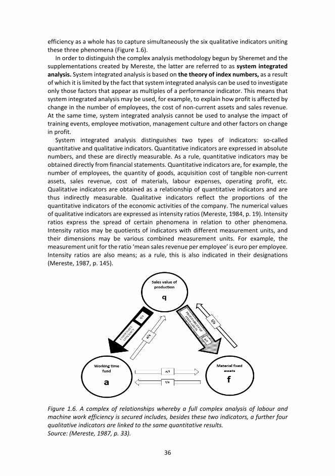
36

efficiency as a whole has to capture simultaneously the six qualitative indicators uniting these three phenomena (Figure 1.6).

In order to distinguish the complex analysis methodology begun by Sheremet and the supplementations created by Mereste, the latter are referred to as system integrated analysis. System integrated analysis is based on the theory of index numbers, as a result of which it is limited by the fact that system integrated analysis can be used to investigate only those factors that appear as multiples of a performance indicator. This means that system integrated analysis may be used, for example, to explain how profit is affected by change in the number of employees, the cost of non-current assets and sales revenue. At the same time, system integrated analysis cannot be used to analyse the impact of training events, employee motivation, management culture and other factors on change in profit.

System integrated analysis distinguishes two types of indicators: so-called quantitative and qualitative indicators. Quantitative indicators are expressed in absolute numbers, and these are directly measurable. As a rule, quantitative indicators may be obtained directly from financial statements. Quantitative indicators are, for example, the number of employees, the quantity of goods, acquisition cost of tangible non-current assets, sales revenue, cost of materials, labour expenses, operating profit, etc. Qualitative indicators are obtained as a relationship of quantitative indicators and are thus indirectly measurable. Qualitative indicators reflect the proportions of the quantitative indicators of the economic activities of the company. The numerical values of qualitative indicators are expressed as intensity ratios (Mereste, 1984, p. 19). Intensity ratios express the spread of certain phenomena in relation to other phenomena. Intensity ratios may be quotients of indicators with different measurement units, and their dimensions may be various combined measurement units. For example, the measurement unit for the ratio ‘mean sales revenue per employee’ is euro per employee. Intensity ratios are also means; as a rule, this is also indicated in their designations (Mereste, 1987, p. 145).

Figure 1.6. A complex of relationships whereby a full complex analysis of labour and machine work efficiency is secured includes, besides these two indicators, a further four qualitative indicators are linked to the same quantitative results. Source: (Mereste, 1987, p. 33).

37

System integrated analysis uses models consisting of multipliable components, referred to as component systems. Component systems consist of at least two components, of which at least one is quantitative and another qualitative. Only components whose product has an independent economic sense may be involved in a single component system. Such an example is the objective of developing a finished goods model in the form of a two-element component system whereby the impact of change in labour efficiency to change in volume of finished goods is measured. In this case, labour efficiency (V) needs to be defined through the volume of finished goods: for instance, the relationship between volume of finished goods (N) and budgeted working time (A):

𝑉𝑉 = 𝑁𝑁𝐴𝐴

. (1.5)

Thus, finished goods may be modelled as a product of the budgeted working time and labour efficiency:

𝑁𝑁 = 𝑅𝑅 × 𝑉𝑉. (1.6)

By replacing the values of one component and leaving the other unchanged, it is possible to obtain knowledge of how a performance indicator (or, volume of finished goods) changes under the impact of the component. Component systems are distinguished from production functions by the fact that, in a component system, a quantitative component functions next to a qualitative component linked to it. In the case of production functions, one quantitative component is next to another quantitative component, which does not directly depend on change in the first component. For example, the Cobb–Douglas production function models finished goods as a function of two variables.

𝑁𝑁 = 𝑎𝑎𝑅𝑅𝛼𝛼𝐶𝐶𝛽𝛽, (1.7)

where A is labour used, C is capital invested and a, α and β are function parameters. In this respect,

𝛼𝛼 + 𝛽𝛽 = 1. (1.8)

The Cobb-Douglas function presupposes that goods manufactured to the use of both capital and labour and their intensity remain stable during the period (Cobb & Douglas, 1928).

In summary, the objective of system integrated analysis is to analyse the various facets of the activities of a company systemically and comprehensively and to provide an overall evaluation of the efficiency of the economic activities of a company. The accomplishment of the objectives of this doctoral thesis also considers the principles of complexness and systemicity, so that efficiency matrices may be used to analyse all the facets of the business activities of a company. The author of the doctoral thesis considers it positive that, despite the fact that the theory of complex analysis was developed under the conditions of a Socialist regime, it was free from ideology. For that reason, the theory above can also be applied today. In the opinion of the author of the thesis, system integrated analysis may be used in the case of manufacturing, trading and service companies alike.

38

1.4 Development of the concept of an efficiency matrix: an historical overview The use of the efficiency matrix and its developments were well known in Estonia from the late 1970s until the 1990s and, to a lesser extent, since the 2000s. The author of doctoral thesis splits the development of the efficiency matrix concept into four periods:

1) 1976–1981: Formation of visual form of an efficiency matrix,2) 1980–1984: Composition of overall efficiency indicators,3) 1984–1990: Rapid development of concept of efficiency matrix,4) 2000–today: Rebirth of efficiency matrix concept.

The following subchapters compose an overview of the pioneering and most considerable research published in these periods. The novelty of the current subchapter is that it is first time this overview has been published in English.

1.4.1 1976–1981: Formation of visual form of an efficiency matrix In 1976, development of economic analysis methodology was included among the major research areas at the Tallinn Polytechnic Institute (Mereste, Vensel, & Straž, 1986, p. 9). By 1981, the visual form of the efficiency matrix was established.

In 1977, Mereste presented for the first time the principles of the matrix approach to the economic efficiency of manufacturing developed at the Faculty of Economics of the Tallinn Polytechnic Institute. Based on that, qualitative indicators linking the major quantitative indicators had to be subjected to permanent control and begin to be affected in a planned manner (Mereste, 1977). Mereste notes at the same time that by limiting the scope to, for example, the main quantitative indicators of a company’s activities, such as goods, working time, profit, wages, cost of materials, non-current assets and current assets, 42 (= 72 – 7) different relationships are formed among them. In the opinion of Mereste, it makes sense to consolidate these relationships into a cross-tabulation that may be referred to as an efficiency matrix. At this time, Mereste in his paper did not yet include a matrix in a visual form. Mereste pointed out in the same paper that at the time there was a lot of literature about analysing labour productivity, cost price and sales profitability, yet, for example, analysis of the profitability of non-current assets and labour and of the labour intensity of materials processing had been carried out at non-existent levels. Thus, in the opinion of Mereste, there was a clear need for a theory to shed light on the internal relationships of a complex of phenomena affecting economic efficiency and on their reciprocal mechanism of action.

In his paper “Ühiskondliku tootmise majandusliku efektiivsuse tõus Eestis 1960–1977” [Rise of the economic efficiency of public manufacturing in Estonia from 1960 to 1977], Mereste (1980) used the matrix approach for the first time. He emphasised that, compared to the qualitative indicators used in the investigation of economic phenomena to date, an economic efficiency indicator should have greater generalisation power and include a greater number of individual phenomena (Mereste, 1980). At the same time, a paper published in the 1980s presents for the first time an efficiency matrix in a visual form (Table 1.6).

39

Table 1.6. General form of an efficiency matrix.

Mereste emphasised that, according to the matrix methodology, the quantitative indicators selected have to be considered in two ways: as components (α) affecting other quantitative indicators and as performance indicators (γ) dependent on the impact of other components (both, quantitative α and qualitative β). In this case, a relationship connecting the variables in the front column (αi), table head (γj) and table field (βij) of the efficiency matrix is formed:

𝛼𝛼𝑝𝑝 × 𝛽𝛽𝑝𝑝𝑖𝑖 = 𝛾𝛾𝑖𝑖. (1.9)

To analyse economic efficiency at national level, Mereste involved six quantitative indicators available from public data:

− gross national product (Q), − national income (P), − total value of tangible fixed assets used in the national economy (F), − aggregated electricity expense (E), − size of population (N), − number of employees engaged in national economy (A).

The fact that an efficiency matrix encompasses and links in an intelligible manner many indicators related to efficiency reduces the problem of selecting qualitative indicators. Mereste refers to the efficiency matrix (Table 1.7) created as an aggregate model of efficiency, that is, a system of simple models consisting of 30 individual models. According to Mereste, a system of simple models is more preferable than a hard-to-understand system of models intertwined in a complicated manner. A system of simple models makes it possible to substantively interpret the results of the analysis obtained on the basis of every individual model. In order to facilitate the reading of an efficiency matrix, Mereste framed the elements whose value should increase as efficiency rises.

Source: (Mereste, 1980), adapted by the author.

40

In his paper published in 1981, Mereste aimed to compare the efficiency levels of six machine factories and shipyards and to ascertain based on the results obtained the ranking of the factories according to the level of the efficiency of manufacturing at a specific point in time (Mereste, 1981). The model involves six quantitative indicators: profit (P), total cost of manufacturing and services (T), cost of finished goods produced (G), amount of manufacturing costs (M), cost of tangible fixed assets (F) and average number of employees per year (A). Thus, for every factory it was possible to form a 6×6 matrix model in which there are 30 qualitative indicators. In an innovation, Mereste engaged in the creation of a structured efficiency matrix, consolidating under the main diagonal all those elements that increase as efficiency rises on the assumption that all the other factors remain the same (Table 1.8).

Table 1.7. Efficiency matrix of national economy.

Source: (Mereste, 1980).

41

Table 1.8. Structured efficiency matrix of a machine factory or shipyard.

Structuring makes paying attention to the elements symmetric with respect to the main diagonal. The issue of the direction of changes in the numerical value of quantitative indicators with growth of efficiency is solved for every pair separately on the assumption that all other matrix elements do not change. For example, by comparing elements 12 (total cost of manufacturing and services to profit) and 21 (profit to total cost of manufacturing and services) in Table 1.8 it is easy to understand that when other conditions remain the same, efficiency can increase only when profit to total cost of manufacturing and services increases. Proceeding analogously, we reach the result that when efficiency increases all five qualitative indicators in the profit column, four qualitative indicators in the total cost of manufacturing and services column must increase (element 12 or total cost of manufacturing and services to profit ratio will diminish when efficiency increases), etc. In this way, it is possible to draw all elements of the matrix that increase with efficiency growth together under the matrix diagonal.

The visual form of structured efficiency matrix presented by Mereste (1981) was widely accepted by researchers. The future studies focused mainly on the investigation of different areas of the efficiency matrix and compiling efficiency matrices for the needs of different industries. The author of this doctoral thesis is of the opinion that on the one hand the form of efficiency matrix can be easily exploited, but on the other hand the practical need of reverse values above the main diagonal of the efficiency matrix could be disputable.

Hereinafter in the thesis, it is tacitly assumed that an efficiency matrix is presented in a structured form, and this is not highlighted separately.

Source: (Mereste, 1981).

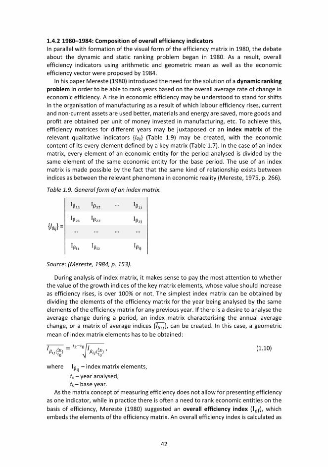
42

1.4.2 1980–1984: Composition of overall efficiency indicators In parallel with formation of the visual form of the efficiency matrix in 1980, the debate about the dynamic and static ranking problem began in 1980. As a result, overall efficiency indicators using arithmetic and geometric mean as well as the economic efficiency vector were proposed by 1984.

In his paper Mereste (1980) introduced the need for the solution of a dynamic ranking problem in order to be able to rank years based on the overall average rate of change in economic efficiency. A rise in economic efficiency may be understood to stand for shifts in the organisation of manufacturing as a result of which labour efficiency rises, current and non-current assets are used better, materials and energy are saved, more goods and profit are obtained per unit of money invested in manufacturing, etc. To achieve this, efficiency matrices for different years may be juxtaposed or an index matrix of the relevant qualitative indicators {Iβij} (Table 1.9) may be created, with the economic content of its every element defined by a key matrix (Table 1.7). In the case of an index matrix, every element of an economic entity for the period analysed is divided by the same element of the same economic entity for the base period. The use of an index matrix is made possible by the fact that the same kind of relationship exists between indices as between the relevant phenomena in economic reality (Mereste, 1975, p. 266).

During analysis of index matrix, it makes sense to pay the most attention to whether the value of the growth indices of the key matrix elements, whose value should increase as efficiency rises, is over 100% or not. The simplest index matrix can be obtained by dividing the elements of the efficiency matrix for the year being analysed by the same elements of the efficiency matrix for any previous year. If there is a desire to analyse the average change during a period, an index matrix characterising the annual average change, or a matrix of average indices {𝐼𝐼𝛽𝛽𝛽𝛽𝛽𝛽����}, can be created. In this case, a geometric mean of index matrix elements has to be obtained:

𝐼𝐼𝛽𝛽𝚤𝚤𝚤𝚤(𝑡𝑡𝜅𝜅𝑡𝑡0)

�������� = �𝐼𝐼𝛽𝛽𝑖𝑖𝑖𝑖(𝑡𝑡𝜅𝜅𝑡𝑡0)

𝑡𝑡𝑘𝑘−𝑡𝑡0 , (1.10)

where Iβij – index matrix elements, tk – year analysed, t0 – base year.

As the matrix concept of measuring efficiency does not allow for presenting efficiency as one indicator, while in practice there is often a need to rank economic entities on the basis of efficiency, Mereste (1980) suggested an overall efficiency index (Ief), which embeds the elements of the efficiency matrix. An overall efficiency index is calculated as

Table 1.9. General form of an index matrix.

Source: (Mereste, 1984, p. 153).

43

the arithmetic mean of the growth indices of efficiency matrix elements, which should increase as efficiency rises:

𝐼𝐼𝑁𝑁𝑝𝑝 =2∑𝐸𝐸′𝛽𝛽𝑖𝑖𝑖𝑖𝑛𝑛2–𝑛𝑛

, (1.11)

where I’βij – growth indices of all the efficiency matrix elements that have to grow as efficiency rises, regardless of whether they grew or decreased in reality, n – number of quantitative indicators in the model.

Formula (1.11) assumes that the growth indices of efficiency matrix elements have been calculated compared to the previous year. If there is a need to obtain the annual average value of an overall efficiency index (Ief���), it may be obtained using the formula (Mereste, 1980):

𝐼𝐼𝑁𝑁𝑝𝑝(𝑡𝑡𝜅𝜅𝑡𝑡0)

�������� = �2∑𝐸𝐸′𝛽𝛽𝑖𝑖𝑖𝑖𝑛𝑛2–𝑛𝑛

𝑡𝑡𝑘𝑘−𝑡𝑡0, (1.12)

where I’βij – underlying growth indices of all efficiency matrix elements that should grow as efficiency rises, regardless of whether they grew or decreased in reality, n – number of quantitative indicators in the model, tk – year analysed, t0 – base year.

Efficiency index means are easy to analyse, since the reasons for their changes are easy to ascertain based on efficiency matrices.

The overall efficiency index Ief constructed by Mereste is the unweighted average of the growth rates of the qualitative indicators used to calculate it. At the same time, the impact of every initial indicator in the model varies in the formation of efficiency. Some indicators (for example, gross national product and national income in Table 1.7) are mostly in the numerator (that is, in effect function) of ratios. Some indicators (for example, the number of employees and the size of population) are mostly in the denominator (that is, in efficiency base function) of ratios. Thus, according to Mereste, it is a bidirectionally balanced weighting system wherein every initial indicator in the model has two integral weights depending on the level of finality of the index as an effect indicator and on its universality as an efficiency base (Mereste, 1980).

Next, Mereste (1981) developed a comparative multiplier matrix (hereinafter: comparative matrix) of elements under the main diagonal of an efficiency matrix, where the indicator, under the main diagonal, for every factory has been divided by the same indicator for the factory serving as a comparison basis (formula 1.13). Any factory analysed whatsoever could serve as the benchmark.

𝑐𝑐′𝑝𝑝𝑖𝑖𝐴𝐴/0 =

𝑇𝑇𝑖𝑖𝑖𝑖𝐴𝐴

𝑇𝑇𝑖𝑖𝑖𝑖0 , (1.13)

where c′ijA/0 – element under the main diagonal of comparative multipliers (growth

index), 𝑎𝑎𝑝𝑝𝑖𝑖𝐴𝐴 – element under the main diagonal of an economic entity analysed (A), 𝑎𝑎𝑝𝑝𝑖𝑖0 – value of the same element under the main diagonal for the same period in an efficiency matrix for the economic entity selected as the benchmark (0).

Next, similarly to the overall efficiency index, Mereste calculated the arithmetic mean of the elements under the diagonal of the comparative matrix, or the overall

44

comparative multiplier of efficiency (comparative multiplier) (formula 1.14), and he arranged factories in the order of the decrease of the comparative multiplier.

𝐶𝐶𝑁𝑁𝑝𝑝𝐴𝐴/0 =

2∑𝑐𝑐′𝑖𝑖𝑖𝑖𝐴𝐴/0

𝑛𝑛2–𝑛𝑛, (1.14)

where c′ijA/0 – values of all the comparative matrix elements that should grow as

efficiency rises, regardless of whether they grew or decreased in reality, n – number of quantitative indicators in the model.

It is important to note that an order obtained in this way does not rest on any measurement result expressed as an absolute number but rather solely on a comparison between economic entities. The value of a comparative multiplier shows how much higher or lower the efficiency levels of manufacturing at an economic entity are compared to the benchmark economic entity. For example, if a comparative multiplier for a factory was 1.2, its level of efficiency was 20% higher than at the factory being compared. If the user of the information would like to determine why the level of efficiency of one factory was higher than that of another, this can be learned from a detailed analysis of the values of the elements of a comparative multiplier matrix. In the opinion of Mereste, those comparative multipliers whose values exceed 100%, should be considered the most important ones.

Mereste emphasises ease of use as the main advantage of his methodology: the methodology may be applied with a limited number of initial data. At the same time, Mereste stresses that the methodology makes it possible to measure efficiency indirectly, rather than directly, since its numerical results depend on the selection of the benchmark. As alternatives to adopting a single specific factory as the benchmark, Mereste recommends considering matrices that characterise the average of factories, standard (that is, corresponding to the national standards applicable at the time) or optimum efficiency levels.

Root (1981) pointed out that indices characterising change in efficiency are multiples, as a result of which it is more appropriate to use the formula of the geometric mean:

𝐼𝐼𝑁𝑁𝑝𝑝𝐺𝐺 = �∏𝐼𝐼′𝛽𝛽𝑖𝑖𝑖𝑖𝑛𝑛2–𝑛𝑛2 , (1.15)

where 𝐼𝐼′β𝑖𝑖𝑖𝑖 – growth indices of all the efficiency matrix elements that should grow as efficiency rises, regardless of whether they grew or decreased in reality, n – number of initial quantitative indicators in the model.

At the same time, Root in his paper also proposed an overall efficiency index formula that may be applied without developing an efficiency matrix by using only the growth indices of all initial indicators.

𝐼𝐼𝑁𝑁𝑝𝑝𝐺𝐺 = �∏ 𝑖𝑖𝑖𝑖𝑛𝑛–(2𝑖𝑖−1)𝑛𝑛

𝑖𝑖=1

𝑛𝑛2–𝑛𝑛2 = �𝑖𝑖1𝑛𝑛−1

𝑛𝑛2–𝑛𝑛2 × �𝑖𝑖2𝑛𝑛−3

𝑛𝑛2–𝑛𝑛2 × … × �𝑖𝑖𝑛𝑛

𝑛𝑛−(2𝑛𝑛−1)𝑛𝑛2–𝑛𝑛2

, (1.16)

where 𝑖𝑖𝑖𝑖 – growth index of quantitative indicator, n – number of quantitative indicators in the model.

The formula (1.16) works well when there is an even number of quantitative indicators (Альвер, 1989). For example, in the case of four quantitative indicators, an efficiency index may be calculated as follows:

45

𝐼𝐼𝑁𝑁𝑝𝑝𝐺𝐺 = �∏ 𝑖𝑖𝑖𝑖4–(2𝑖𝑖−1)4

𝑖𝑖=16

= �𝑖𝑖136 × �𝑖𝑖21

6 × �𝑖𝑖3−16 × �𝑖𝑖4−3

6 . (1.17)

If the number of quantitative indicators is an odd number, the impact of the middle indicator will be left out of the calculation of an efficiency index. For example, in the case of five quantitative indicators, an efficiency index may be calculated as follows:

𝐼𝐼𝑁𝑁𝑝𝑝𝐺𝐺 = �∏ 𝑖𝑖𝑖𝑖5–(2𝑖𝑖−1)5

𝑖𝑖=110

= �𝑖𝑖1410 × �𝑖𝑖22

10 × �𝑖𝑖3010 × �𝑖𝑖4−2

10 × �𝑖𝑖5−410 . (1.18)

As noted above, the part of every quantitative indicator in a model is different in the formation of efficiency: some indicators are mostly in effect function (in the numerator of ratios) and other indicators are mostly in efficiency base function (in the denominator of ratios). In the case of an odd-numbered quantity of quantitative indicators, the middle indicator is equally in effect and efficiency base functions, as a result of which its impact on the calculation of an efficiency index is eliminated. Therefore, in the opinion of the author of the thesis, it makes sense to involve an even number of quantitative indicators in the analysis of efficiency.

Both arithmetic and geometric mean are quantity averages whose numerical value depends on every individual value in the statistical series. The numerical values of various means obtained from the same numbers vary, with the value of a geometric mean always less than the value of an arithmetic mean. Thus, the relationship is

𝐼𝐼𝑁𝑁𝑝𝑝𝐺𝐺 < 𝐼𝐼𝑁𝑁𝑝𝑝 (1.19)

Mereste (1984, p. 157) concedes that, when a geometric mean is calculated, obtaining an efficiency index technically has some advantages in terms of calculation and analysis; however, this considers that, despite these advantages, there is no direct need to use a geometric mean, since the main advantage of using an arithmetic mean – the convenience of calculating it – outweighs its drawbacks. Tinits (Тинитс, 1985) pointed out that the arithmetic mean had the drawback that in certain instances the efficiency index may be greater than 1 or 100% (that is, indicating a rise in efficiency) if both the indices under the main diagonal of a structured efficiency matrix and the indices on top of the main diagonal of the same efficiency matrix (which are reverse values of the indices under the diagonal) are used. Therefore, the use of the arithmetic mean has to consider that the result of the efficiency index depends on whether indices under or on top of the main diagonal of a structured efficiency matrix are used:

𝐼𝐼𝑁𝑁𝑝𝑝𝑁𝑁𝑘𝑘

𝑁𝑁0�≠ 1

𝐸𝐸𝑒𝑒𝑒𝑒

𝑡𝑡0𝑡𝑡𝑘𝑘�

. (1.20)

No such problem arises when the geometric mean is used. In this case, an efficiency index calculated on the basis of the elements under the diagonal of a structured efficiency matrix equals the reverse value of the efficiency index obtained based on the elements on top of the diagonal.

𝐼𝐼𝐺𝐺𝑁𝑁𝑝𝑝𝑁𝑁𝑘𝑘

𝑁𝑁0�= 1

𝐸𝐸𝐺𝐺𝑒𝑒𝑒𝑒

𝑡𝑡0𝑡𝑡𝑘𝑘�

(1.21)

Relationships (1.20) and (1.21) also apply in the case of the calculation of efficiency comparative multipliers. Thus, when calculating both the overall efficiency index and the

46

overall comparative multiplier, it is appropriate to use the geometric mean. Since today calculations are performed using computer software solutions, not manually, it is not sensible in the opinion of the author of the thesis to prefer the arithmetic mean merely because of the convenience of calculating it.

Vensel (1984) used the concept of an efficiency matrix in the development of an economic efficiency vector (efficiency vector indicator) of manufacturing. In the case of the efficiency vector indicator methodology, the following properties of an efficiency matrix are important:

1) the elements of the diagonal of an efficiency matrix equal 1,2) elements located symmetrically in relation to the main diagonal (qualitative

indicators) are reverse values of one another,3) an efficiency matrix consists of linearly dependent column and row vectors.

Based on these properties, Vensel (1984, p. 44) concluded that the consideration of just a single qualitative indicator vector, which Vensel referred to as the efficiency vector, was sufficient for analysing the efficiency of a business entity. For this, efficiency vector elements should be qualitative indicators for which the numerator (effect) in the calculation formula is a performance indicator and the denominator (efficiency base) is a cost- or resource-type quantitative indicator. Since efficiency vector elements are qualitative indicators with different economic content and measurement units, these need to be normalised (common-sized), and then generalising efficiency vector level indicators may be developed and analysed. Interpretation of results obtained in this way should consider that all indicators obtained by means of normalisation and the change therein are manifested in comparable dimensionless ratios that may be interpreted as spheres or points.

On the basis of the above the author of the doctoral thesis is of the opinion that overall efficiency index and overall comparative multiplier based on geometric mean deserve further consideration when ranking economic entities. The main advantage of those indicators is that they comprise all the indices below the main diagonal of efficiency matrix (not just a single vector, as is the case of an efficiency vector indicator). It should be noted that usage of geometric mean has a limitation in that all the elements of index matrix and comparative multiplier matrix have to have positive values. In the case of index matrix and comparative multiplier matrix including negative element(s), the arithmetic mean could be regarded as an alternative option.

1.4.3 1984–1990: Rapid development of concept of efficiency matrix 1984–1990 can be summarised as a period of rapid development of the efficiency matrix concept. The main milestones can be summarised as follows:

− introduction of the efficiency field concept, − analysis of the relationships between the elements of the efficiency matrix and

usage of the chain-linking method to distribute absolute increment, − discussion of the sequence of quantitative indicators included in the efficiency

matrix, − introduction of efficiency matrix analysis by subareas, − making suggestions of modified and concentric matrix models, − compilation of efficiency matrices to research specific facets of economic

entities (usage of current and fixed assets and labour, fulfilment of budget, etc.), − matrix modelling started to spread to other Soviet republics and its satellite

states.

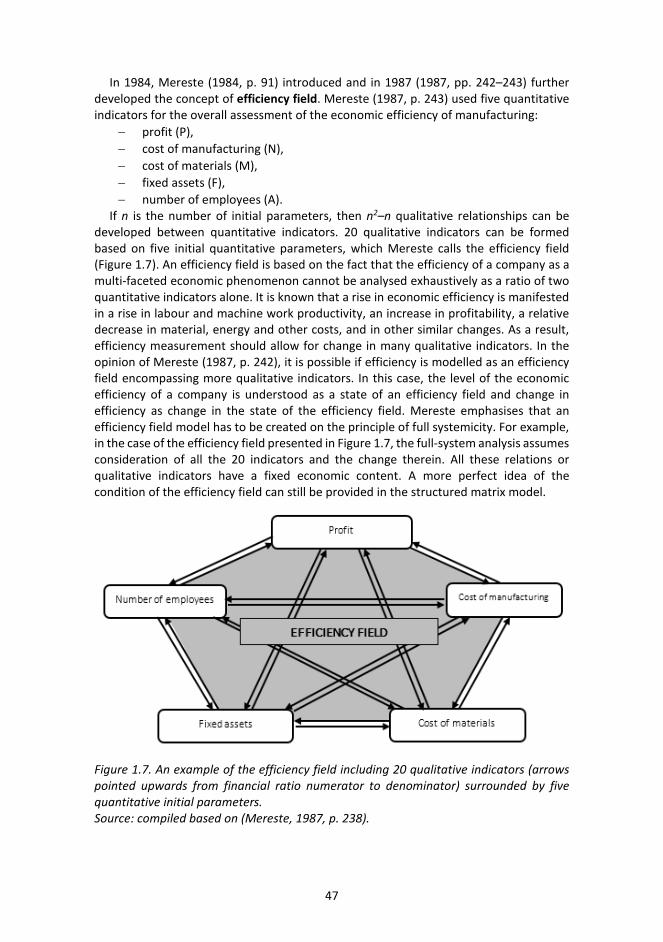
47

In 1984, Mereste (1984, p. 91) introduced and in 1987 (1987, pp. 242–243) further developed the concept of efficiency field. Mereste (1987, p. 243) used five quantitative indicators for the overall assessment of the economic efficiency of manufacturing:

− profit (P), − cost of manufacturing (N), − cost of materials (M), − fixed assets (F), − number of employees (A).

If n is the number of initial parameters, then n2–n qualitative relationships can be developed between quantitative indicators. 20 qualitative indicators can be formed based on five initial quantitative parameters, which Mereste calls the efficiency field (Figure 1.7). An efficiency field is based on the fact that the efficiency of a company as a multi-faceted economic phenomenon cannot be analysed exhaustively as a ratio of two quantitative indicators alone. It is known that a rise in economic efficiency is manifested in a rise in labour and machine work productivity, an increase in profitability, a relative decrease in material, energy and other costs, and in other similar changes. As a result, efficiency measurement should allow for change in many qualitative indicators. In the opinion of Mereste (1987, p. 242), it is possible if efficiency is modelled as an efficiency field encompassing more qualitative indicators. In this case, the level of the economic efficiency of a company is understood as a state of an efficiency field and change in efficiency as change in the state of the efficiency field. Mereste emphasises that an efficiency field model has to be created on the principle of full systemicity. For example, in the case of the efficiency field presented in Figure 1.7, the full-system analysis assumes consideration of all the 20 indicators and the change therein. All these relations or qualitative indicators have a fixed economic content. A more perfect idea of the condition of the efficiency field can still be provided in the structured matrix model.

Figure 1.7. An example of the efficiency field including 20 qualitative indicators (arrows pointed upwards from financial ratio numerator to denominator) surrounded by five quantitative initial parameters. Source: compiled based on (Mereste, 1987, p. 238).

48

According to Mereste (1984, p. 58), an efficiency indicator has to have two components: it has to be made up of both an intensity indicator (for example, quantity of goods per hour of work) and an efficiency criterion (for example, number of hours of work). An efficiency criterion may be a quantitative variable as well as a qualitative variable. Mereste (1984, p. 80) also points out that indices characterise relative change in components; however, there is also need to solve problems that presuppose the determination of the variance of components in absolute numbers, or as an absolute increment (for example, in units of money). For this, it is necessary to ascertain whether the achievement of the objectives of analysis requires regarding components as co-varying or whether their effect may be considered in simpler terms on the assumption that components change in a certain order. Although the latter approach provides more conditional results, in the opinion of Mereste, in practice there are often cases where there is a desire to observe simultaneously-changing components as if they were changing consecutively and independently. In this case, the chain-linking method may be used to distribute the absolute increment.

The chain-linking method is a modification of the index method. Whereas the numerical values of an index are obtained as a relationship of the indicators in the formula, the chain-linking method is used to obtain the differences between the same amounts. Indeed, the latter are considered as the absolute variances of the relevant components. Volt and Renter (1986, p. 5) classify the principles of the distribution of absolute increment into three groups:

1) The principle of direct breakdown where increment is divided betweencomponents directly (in the case of the first component, its impact isconsidered in isolation; in the case of the subsequent components, themutual synergies of the components are also considered).

2) Principle of incomplete breakdown where the increment created by thesynergy between components is left undistributed among components (thatis, the isolated variance of each component is obtained).

3) Complete breakdown, in the case of which both, each component’s isolatedvariance is calculated and synergies are allocated between all thecomponents (for example, equally).

Volt and Renter (1986, p. 7) emphasised that the use of the chain-linking method has the order of the replacement of components. They recommended replacing first indicators in physical units and then indicators in monetary units. In the case of multiple indicators in physical or monetary units, they recommend first replacing quantitative variables (obtained by means of addition or subtraction) and then qualitative indicators (obtained by means of multiplication and division).

Rammo and Volt (1985, pp. 5–7) used a 10×10 square matrix to investigate the efficiency of manufacturing activities, which they call base matrix. In order of finality, the following quantitative indicators were included in the base matrix:

− number of employees, − labour expenses, − current assets used in manufacturing, − fixed assets used in manufacturing, − total assets used in manufacturing, − cost of manufacturing, − value of goods manufactured (output produced during a time period, which has

been sold already or is intended for sale or use for own consumption),

49

− sales value of products, − value of total production (irrespective of the degree of completeness), − profit.

On the basis of the base matrix, Rammo and Volt composed three sub-matrices: efficiency matrices of fixed assets and current assets, and of usage of labour. Seven qualitative indicators were used for analysing the efficiency of fixed assets usage, which are listed in order of finality: value of goods produced, energy costs, machine-hours, cost of active fixed assets, cost of passive fixed assets, total cost of fixed assets and number of employees. Machines, equipment and other inventory are mainly included in the active fixed assets, while land, buildings and facilities are among the passive fixed assets. The positioning of energy costs in second place is justified by the fact that an increase in energy consumption must be accompanied by a more intensive use of fixed assets.

The outcome indicator in the efficiency matrix of current assets usage, according to Rammo and Volt, is the value of products sold. The resource indicators are raw materials, direct materials, indirect materials, supplies and fuel related costs, as well as the number of employees.

The outcome indicator in the efficiency matrix of labour usage is the total value of production while input indicators are wage per hour, daily wage, annual wage, number of man-hours, number of working days and number of employees. Daily wage includes hourly wages and additional remuneration (e.g. for working overtime). In addition to daily wages, annual wage includes all bonuses and other remuneration paid to employees either monthly or for longer periods.

Vensel (1985a, pp. 62–69) presents a 7×7 efficiency matrix that may be used for analysing the efficiency of the use of labour. The quantitative indicators involved by Vensel include:

− average number of employees, − man-days used, − man-hours used, − cost of employees’ annual pay, − cost of employees’ daily pay, − cost of employees’ hourly pay, − cost of finished goods.

Based on seven quantitative indicators, 42 qualitative indicators may be calculated; however, Vensel focused on 21 indicators of the efficiency field and omitted the indicators in the reverse efficiency field. For the analysis of the efficiency of the use of labour, he developed a theoretical numerical example using the values of quantitative indicators of the base and reporting periods compared. For this, Vensel developed three efficiency fields: a base period efficiency field, a reporting period efficiency field and an index matrix obtained by dividing the relevant indicators of the reporting and base periods.

In addition, Vensel (1985b, p. 11) emphasises that all the elements of an efficiency matrix are interlinked and that the elements in the first column of the matrix equal the product of the qualitative indicators under the main diagonal of the (sub)matrix. This approach makes it possible to analyse change in the value of the elements in the first column by component. This means that the efficiency matrix presented in Table 1.8 is subject to a relationship that characterises the formation of profit earned by an employee across five components:

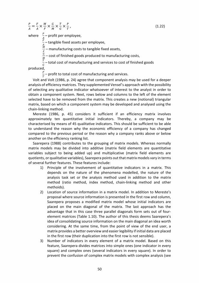
50

𝑃𝑃𝐴𝐴

= 𝐹𝐹𝐴𝐴

× 𝑀𝑀𝐹𝐹

× 𝐺𝐺𝑀𝑀

× 𝑇𝑇𝐺𝐺

× 𝑃𝑃𝑇𝑇

, (1.22)

where 𝑃𝑃𝐴𝐴

– profit per employee,𝐹𝐹𝐴𝐴

– tangible fixed assets per employee,𝑀𝑀𝐹𝐹

– manufacturing costs to tangible fixed assets,𝐺𝐺𝑀𝑀

– cost of finished goods produced to manufacturing costs,𝑇𝑇𝐺𝐺

– total cost of manufacturing and services to cost of finished goodsproduced,

𝑃𝑃𝑇𝑇

– profit to total cost of manufacturing and services.Volt and Volt (1986, p. 24) agree that component analysis may be used for a deeper

analysis of efficiency matrices. They supplemented Vensel’s approach with the possibility of selecting any qualitative indicator whatsoever of interest to the analyst in order to obtain a component system. Next, rows below and columns to the left of the element selected have to be removed from the matrix. This creates a new (notional) triangular matrix, based on which a component system may be developed and analysed using the chain-linking method.

Mereste (1986, p. 45) considers it sufficient if an efficiency matrix involves approximately ten quantitative initial indicators. Thereby, a company may be characterised by means of 45 qualitative indicators. This should be sufficient to be able to understand the reason why the economic efficiency of a company has changed compared to the previous period or the reason why a company ranks above or below another on the efficiency ranking list.

Saarepera (1988) contributes to the grouping of matrix models. Whereas normally matrix models may be divided into additive (matrix field elements are quantitative variables subject to being added up) and multiplicative (matrix field elements are quotients, or qualitative variables), Saarepera points out that matrix models vary in terms of several further features. These features include:

1) Principle of the involvement of quantitative indicators in a matrix. Thisdepends on the nature of the phenomena modelled, the nature of theanalysis task set or the analysis method used in addition to the matrixmethod (ratio method, index method, chain-linking method and othermethoids).

2) Location of source information in a matrix model. In addition to Mereste’sproposal where source information is presented in the first row and column,Saarepera proposes a modified matrix model whose initial indicators areplaced on the main diagonal of the matrix. The last approach has theadvantage that in this case three parallel diagonals form sets out of four-element matrices (Table 1.10). The author of this thesis deems Saarepera’sidea of consolidating source information on the main diagonal an idea worthconsidering. At the same time, from the point of view of the end user, amatrix provides a better overview and easier legibility if initial data are placed in the first row (their duplication into the first row is not sensible).

3) Number of indicators in every element of a matrix model. Based on thisfeature, Saarepera divides matrices into simple ones (one indicator in everysquare) and complex ones (several indicators in every square). In order toprevent the confusion of complex matrix models with complex analysis (see

51

subhapter 1.3), the author of the thesis recommends classifying matrices into simple and composite matrices based on the number of indicators in every cell.

Saarepera believes that the model proposed by Mereste prompts the question of whether and what kind of causal relationships exist between the quantitative indicators of the efficiency matrices proposed by Mereste and of whether they may be presented as functional, as is done in component analysis. Saarepera also points out that although in the case of the concept proposed by Mereste the ranking of quantitative indicators is important, no attention is devoted to whether quantitative indicators have an intersection or not. Thus, in her opinion, cause-and-effect relationships may also be analysed in pairs. Saarepera does not accept the criticism, levelled at Mereste’s matrix model, that the practicability of using such models is doubtful due to the large number of qualitative indicators. Saarepera also agrees that an efficiency matrix is suitable for the investigation of an efficiency field and that the relationships between quantitative indicators should be justified in terms of the logic of the phenomena.

Table 1.10. An example of modified matrix model.

Source: (Saarepera, 1988, p. 50).

Saarepera proposes the concept of concentric matrix models whereby the object of analysis is two quantitative variables with a complex structure mutually in a relationship of the cause-and-effect type. Saarepera assumes that both quantitative indicators with a complex structure may be considered as general populations and grouped into subpopulations. There must be no shared portions between subpopulations, which makes it possible to use the principle of a subsequent amount when involving quantitative indicators in a model. Subpopulations simultaneously represent components that affect the formation of both the general population and the values of index matrix elements. If causal relationships exist between two general populations (for example, the value of goods and the number of employees), there are also causal relationships between the subpopulations of the two general populations. In the opinion of Saarepera, differences in changes in subpopulations and their causes compared to

52

changes among general populations are indeed of the greatest interest to analysts. In addition, this model may involve a third quantitative variable, in the case of which the subsequent amount principle is not applied. A concentric matrix model based on three quantitative indicators (sales value of goods, number of employees and total assets) is presented in Table 1.11. This model divides the sales value of finished goods and total assets into subpopulations. The value of goods breaks down into profit, labour expenses and cost of materials as well as the current assets and non-current assets of the total assets.

Table 1.11. Example of concentric matrix model.

Source: (Saarepera, 1988, p. 53).

To analyse how the profit of a company is formed and distributed, Tammeraid and Teearu (1988) developed a 20×20 efficiency matrix where the first six quantitative indicators were resource indicators. The rest of the 14 quantitative indicators characterised various levels of income and profit and were involved in the matrix according to the subsequent amount principle, whereby each subsequent indicator was smaller than the previous one by some cost. In the opinion of the author of this thesis, it is a very detailed efficiency matrix, and it would be easier to replace it with a vertical income statement analysis.

Root (1987, pp. 12–20) compiled an efficiency matrix with the purpose of analysing the dynamics and fulfilment of the plan (budget). Output indicators were profit and sales, while input indicators were cost of raw materials and indirect materials, direct labour expenses and man-hours. Root analysed the average levels of qualitative indicators and the changes in them. On this basis, it is possible to build up six matrices with the following qualitative indicators:

− average levels in the base period, − average target levels, − average levels in the accounting period,

53

− planned changes in average levels (reference basis is the base period), − actual changes in average levels (reference basis is the base period), − fulfilment of average target levels (reference basis is the target).

Elements of the new matrices can be compared to each other. For example, it is possible to analyse the base period, plan and accounting period return on sales (profit/sales) and the direction and intensity of the dynamics of change.

Alver and Järve (1987) studied the trading efficiency of retail stores. The authors emphasised the importance of the sequence of quantitative indicators included in the matrix – profit, total income, sales, operating expenses, fixed assets used in manufacturing – and refer to the causal connections between the indicators. Alver and Järve refer to profit as a passive indicator or totally influenced by other quantitative indicators. Fixed assets are fully in the active function, or influence the phenomena above it in the ranking list. The efficiency matrix by Alver and Järve is presented in Table 1.12.

Table 1.12. An example of a retail store efficiency matrix.

Source: (Alver & Järve, 1987).

Alver and Järve (1989) also created a 9×9 matrix model of the key indicators of retail stores, where they expanded the previous efficiency matrix with four new quantitative indicators: labour expenses, working time, selling space and number of employees (Table 1.13). This model facilitates obtaining a more profound analysis of resource usage. Additionally, Alver and Järve introduced six areas in their efficiency matrix that could be analysed independently (Table 1.13):

1) I: Indicators of changes in the structure of results,2) II: Indicators of the efficiency of expenses,3) III: Indicators of changes in relationships between results and resources,4) IV: Indicators of changes in the structure of expenses,5) V: Indicators of changes in relationships between expenses and resources,6) VI: Indicators of changes in the structure of resources.

54

Table 1.13. Efficiency matrix of retail stores’ performance.

Source: (Alver & Järve, 1989).

55

By applying the principle of systemicity and hierarchicalness, Vensel (1988) developed a composite evaluation model for the economic activities of a company based on matrix modelling (Appendix 1). The model shows that a system of complex evaluation based on an efficiency matrix moves in two directions. One direction is the calculation of a overall efficiency index, based on which an abstract assessment may be provided as to the economic activities of a company during a period analysed by comparing the indicator obtained to previous periods, a planned-for efficiency indicator or other companies. Another direction is the general analysis of the economic activities of a company and the ascertainment of problems requiring investigation that is more detailed. To achieve the latter, inter-element component analysis may be used; based on it, more detailed instructions may be developed for the solution of problem areas. The author of this thesis would like to point out that, because of the principle of systemicity, half of the matrices in Appendix 1 are duplicates and that in reality a set includes ten matrices carrying information with various content.

Vensel’s system of the formation of complex evaluation stipulates that an efficiency matrix consists of five quantitative indicators: profit, value of goods manufactured, cost of materials, fixed assets and number of employees. Based on every quantitative indicator in an efficiency matrix, four more detailed matrix models, referred to by Vensel as analysis matrices, may be developed. Thus, based on this model, an overall evaluation of the economic activities of a company may be provided using 20 analytical matrices.

Tosso (1990) used an efficiency matrix as a point of departure for analysing and managing working efficiency. He reached the conclusion that an efficiency matrix is sufficient for the determination of the levels of working efficiency and its constituents (labour and machine work efficiencies) yet insufficient for the management thereof. Lastly, it is important to understand the economic, psychophysiological and social factors that affect working efficiency. For example, labour efficiency may be affected by the health status of employees, their motivation and other factors.

Luur (1990) researched the problems of using the matrix model to measure the dynamics of the economic efficiency of export and import activities of 12 developed capitalist countries between 1960 and 1985.

In the opinion of the author of the doctoral thesis it is substantial that the researchers attained mutual agreement that the principle of the systemicity and sequence of quantitative indicators included in the matrix distinguish efficiency matrices from other matrix models. Therefore, the concentric matrix model cannot be considered as an efficiency matrix. The author of the doctoral thesis agrees that it is technically possible to compile efficiency matrices using an unlimited number of initial quantitative indicators; however, 10 quantitative indicators are sufficient, as 45 qualitative indicators can be calculated and analysed based on these.

It is noteworthy that matrix modelling started to spread internationally during this period, though primarily in the Soviet Union and its satellite states due to political situation. According to Kala (2013) during, in addition to Estonia and Russia, this methodology was introduced in other Soviet republics in the 1980s (e.g. Belarus, Kazakhstan, Armenia and Georgia), as well as in Czechoslovakia, the German Democratic Republic and even Japan. In the mid-1980s, the USSR State Planning Committee ordered the comparative efficiency analysis of the economies of leading socialist countries based on matrix modelling.

56

1.4.4 2000–today: Rebirth of efficiency matrix concept In 1990s there were no significant research papers that further developed the efficiency matrix concept. It was probably related to the economic transformation, which began in 1991. Probably it was not considered reasonable to analyse financial data collected in the Soviet period, and there were not enough new data. Matrix modelling was reintroduced again in the 2000s.

Vensel (2001, p. 66) built up an efficiency matrix to analyse the performance of commercial banks, where the quantitative indicators in descending order of finality were:

− total assets, − equity, − income generating assets (receivables from customers and other commercial

banks, and securities), − interest income, − net interest income, − profit before taxes, − net profit.

At first Vensel drafted the annual consolidated balance sheets and income statements of Estonian commercial banks for period of 1994–1999 in order to construct the efficiency matrix. The years to be analysed were 1997 and 1999 and the base year 1994. Since profitability indicators in 1998 were negative, Vensel omitted this year from the analysis. Hence, five indicators were calculated for every element of the efficiency matrix:

− 1994 level, − 1997 level, − 1997 base growth rate (1997/1994), − 1999 level, − 1999 base growth rate (1999/1994).

Kalle (2007, p. 42) developed an index matrix for the evaluation of productivity level (Table 1.14). In order to distinguish a matrix of evaluation indices from the index matrix presented in Table 1.9 more clearly, the author of the thesis will refer to the matrix created by Kalle as evaluation matrix hereinafter. Evaluation matrix elements are the actual and planned-for values of the indicator for the productivity chosen by the analyst (for example, labour productivity) during the period analysed and periods preceding it as well as the maximum, minimum, average and optimum values for the period analysed. In the opinion of Kalle, the most important indices have been highlighted in the matrix. An evaluation matrix may be used at the level of both subunits and companies. In the opinion of the author of this thesis, the matrix developed by Kalle is suitable if the objective of analysis is the detailed investigation of a specific quantitative or qualitative indicator(s), since in the case of a 10×10 matrix 45 indices (and an identical quantity of reverse values of these indices) may be calculated. Since an evaluation matrix does not strive to analyse efficiency, it does not matter in which order initial indicators are involved in the matrix model.

57

Table 1.14. Index matrix for the evaluation of productivity level.

Note: Act – actual, Bud – budget (plan), Max – maximum, Min – minimum, Ave – average, Opt – Optimal value, t–period analysed, t–1 – previous period, n – any previous period Source: (Kalle, 2007, p. 42).

Today, development of the efficiency matrix methodology continues to be pursued at Tallinn University of Technology. The first English-language review papers on matrix analysis methodology were published by Startseva and Alver (2011) and by Siimann (2011).

Startseva, Zahharov and Alver (2012) used matrix analysis in analysing the efficiency of a manufacturing company. For this, they used one output indicator (labour intensity) and three input indicators (production space, number of operators and duration of the process). Internal efficiency analysis was also continued by Startseva in her doctoral thesis (Стаpцева, 2016) showing opportunities for the use of complex analysis, using the examples of the technological system of an industrial company and of the enhancement of the operations of an electronic document service group.

Siimann and Alver (2015) used an efficiency matrix to analyse change in profit per employee using the example of Estonia’s small and medium-sized information technology and telecommunications companies from 2009 to 2013. The the formation of an efficiency matrix (Table 1.15) four input indicators (number of employees, owners’ equity, financial liabilities (loans) and operating expenses) and two output indicators (earnings before taxes and net sales) were used. The paper focused on the elements under the main diagonal of the efficiency matrix (components 12, 23, 34, 45 and 56),

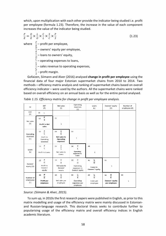
58

which, upon multiplication with each other provide the indicator being studied i.e. profit per employee (formula 1.23). Therefore, the increase in the value of each component increases the value of the indicator being studied. 𝑃𝑃𝐸𝐸

= 𝑂𝑂𝐸𝐸

× 𝐿𝐿𝑂𝑂

× 𝐶𝐶𝐿𝐿

× 𝑆𝑆𝐶𝐶

× 𝑃𝑃𝑆𝑆 (1.23)

where 𝑃𝑃𝐸𝐸

– profit per employee,𝑂𝑂𝐸𝐸

– owners’ equity per employee,𝐿𝐿𝑂𝑂

– loans to owners’ equity,𝐶𝐶𝐿𝐿

– operating expenses to loans,𝑆𝑆𝐶𝐶

– sales revenue to operating expenses,𝑃𝑃𝑆𝑆 – profit margin.

Gofaizen, Siimann and Alver (2016) analysed change in profit per employee using the financial data of four major Estonian supermarket chains from 2010 to 2014. Two methods – efficiency matrix analysis and ranking of supermarket chains based on overall efficiency indicator – were used by the authors. All the supermarket chains were ranked based on overall efficiency on an annual basis as well as for the entire period analysed.

Table 1.15. Efficiency matrix for change in profit per employee analysis.

Source: (Siimann & Alver, 2015).

To sum up, in 2010s the first research papers were published in English, as prior to this matrix modelling and usage of the efficiency matrix were mainly discussed in Estonian- and Russian-language research. This doctoral thesis seeks to contribute further to popularising usage of the efficiency matrix and overall efficiency indices in English academic literature.

59

1.4.5 Synthesis of researches about efficiency matrix modelling and its developments to date This subchapter briefly generalises the key concepts of matrix modelling, focusing mainly on terms linked to efficiency evaluation. Figure 1.8 has been created for the better visualisation, and this consolidates the main concepts linked to efficiency matrix modelling and the relationships between them.

Matrix modelling may be used in the course of both complex and system integrated analyses. Efficiency evaluation has to be based on the principles of system integrated analysis, since its main prerequisite is compliance with the requirement of full systemicity.

The author of this thesis classifies the models of a concentric matrix and an evaluation matrix as complex analysis, since their objective is not adherence to the principle of full systemicity. A concentric matrix is used to investigate 2–3 quantitative variables mutually in a relationship of the cause-and-effect type, two of which have to be divisible into subpopulations. There must be no shared portions between subpopulations, as a result of which the principle of subsequent amount may be used when involving quantitative indicators in a model. An evaluation matrix is suitable for the detailed investigation of the dynamics of a single specific quantitative or qualitative indicator.

The creation of an efficiency field presupposes full systemicity, which allows for change in many qualitative indicators, since the efficiency of an economic entity as a multi-faceted economic phenomenon cannot be analysed exhaustively as a ratio of two quantitative indicators alone. In this case, the level of the economic efficiency of an economic entity is understood as a state of an efficiency field and change in efficiency as change in the state of the efficiency field. An efficiency field is made up of qualitative indicators whose value increases as efficiency rises. A reverse efficiency field consists of reverse values of efficiency field indicators.

An efficiency field is universal and suitable for use at the level of department, business segment, company, group, field of activity, country and geographical region.

A better overview is provided by the cross-tabulation of the relationships in an efficiency field and in its reverse field, which is referred to as efficiency matrix. In a structured efficiency matrix, all those elements that should increase as efficiency rises – on the assumption that all the other indicators remain the constant – are consolidated under the main diagonal. On a regular efficiency matrix, all quantitative initial indicators are presented in the first row and column of the matrix. Every quantitative indicator is considered in two ways: as a component affecting other quantitative indicators and as a performance indicator depending on the impact of other components (both quantitative and qualitative). In a modified efficiency matrix, quantitative indicators are placed on the main diagonal. In this case, sets form out of four-element matrices on the parallel diagonal.

Efficiency matrices may be classified as simple or compound matrices depending on whether every matrix element consists of a single or multiple indicators. In the case of multi-indicator matrices, an element consists of values of various periods of a qualitative indicator and, additionally, may display changes in this qualitative indicator over time.

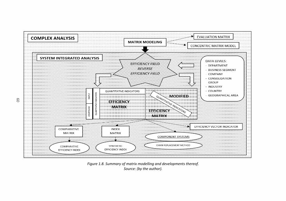
60

Figure 1.8. Summary of matrix modelling and developments thereof. Source: (by the author).

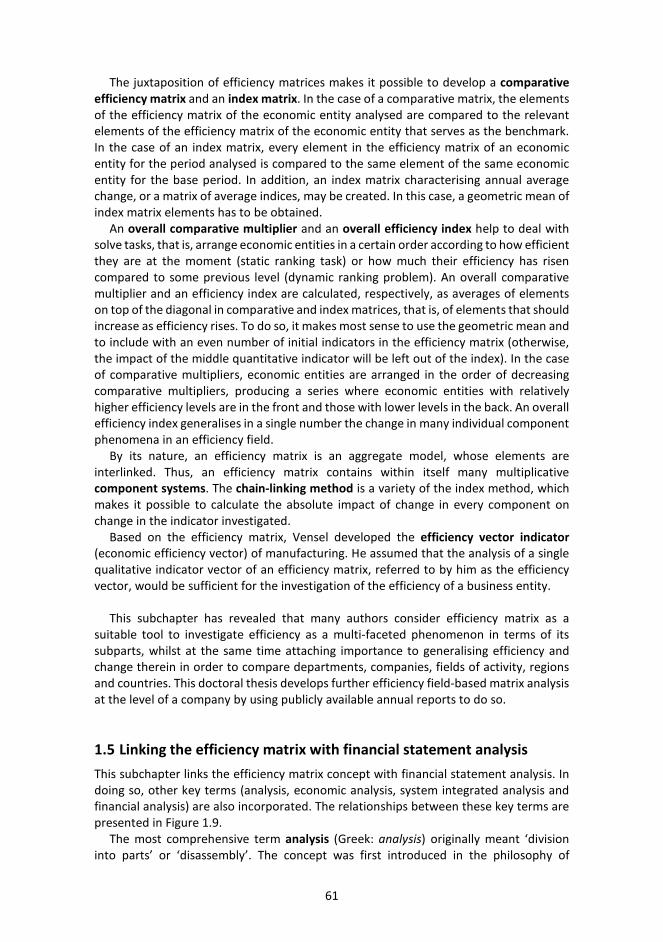
61

The juxtaposition of efficiency matrices makes it possible to develop a comparative efficiency matrix and an index matrix. In the case of a comparative matrix, the elements of the efficiency matrix of the economic entity analysed are compared to the relevant elements of the efficiency matrix of the economic entity that serves as the benchmark. In the case of an index matrix, every element in the efficiency matrix of an economic entity for the period analysed is compared to the same element of the same economic entity for the base period. In addition, an index matrix characterising annual average change, or a matrix of average indices, may be created. In this case, a geometric mean of index matrix elements has to be obtained.

An overall comparative multiplier and an overall efficiency index help to deal with solve tasks, that is, arrange economic entities in a certain order according to how efficient they are at the moment (static ranking task) or how much their efficiency has risen compared to some previous level (dynamic ranking problem). An overall comparative multiplier and an efficiency index are calculated, respectively, as averages of elements on top of the diagonal in comparative and index matrices, that is, of elements that should increase as efficiency rises. To do so, it makes most sense to use the geometric mean and to include with an even number of initial indicators in the efficiency matrix (otherwise, the impact of the middle quantitative indicator will be left out of the index). In the case of comparative multipliers, economic entities are arranged in the order of decreasing comparative multipliers, producing a series where economic entities with relatively higher efficiency levels are in the front and those with lower levels in the back. An overall efficiency index generalises in a single number the change in many individual component phenomena in an efficiency field.

By its nature, an efficiency matrix is an aggregate model, whose elements are interlinked. Thus, an efficiency matrix contains within itself many multiplicative component systems. The chain-linking method is a variety of the index method, which makes it possible to calculate the absolute impact of change in every component on change in the indicator investigated.

Based on the efficiency matrix, Vensel developed the efficiency vector indicator (economic efficiency vector) of manufacturing. He assumed that the analysis of a single qualitative indicator vector of an efficiency matrix, referred to by him as the efficiency vector, would be sufficient for the investigation of the efficiency of a business entity.

This subchapter has revealed that many authors consider efficiency matrix as a suitable tool to investigate efficiency as a multi-faceted phenomenon in terms of its subparts, whilst at the same time attaching importance to generalising efficiency and change therein in order to compare departments, companies, fields of activity, regions and countries. This doctoral thesis develops further efficiency field-based matrix analysis at the level of a company by using publicly available annual reports to do so.

1.5 Linking the efficiency matrix with financial statement analysis This subchapter links the efficiency matrix concept with financial statement analysis. In doing so, other key terms (analysis, economic analysis, system integrated analysis and financial analysis) are also incorporated. The relationships between these key terms are presented in Figure 1.9.

The most comprehensive term analysis (Greek: analysis) originally meant ‘division into parts’ or ‘disassembly’. The concept was first introduced in the philosophy of

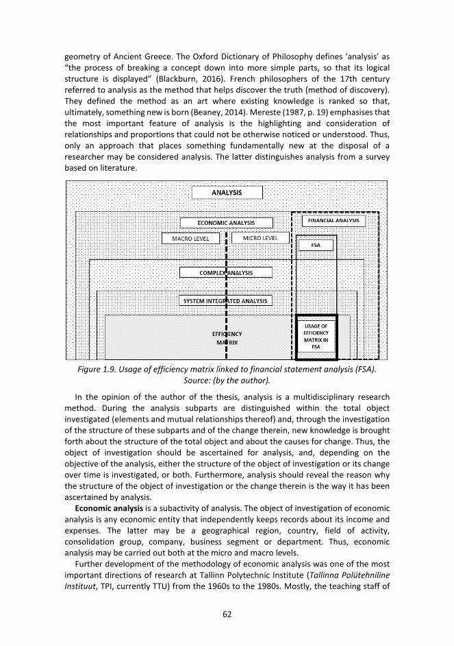
62

geometry of Ancient Greece. The Oxford Dictionary of Philosophy defines ‘analysis’ as “the process of breaking a concept down into more simple parts, so that its logical structure is displayed” (Blackburn, 2016). French philosophers of the 17th century referred to analysis as the method that helps discover the truth (method of discovery). They defined the method as an art where existing knowledge is ranked so that, ultimately, something new is born (Beaney, 2014). Mereste (1987, p. 19) emphasises that the most important feature of analysis is the highlighting and consideration of relationships and proportions that could not be otherwise noticed or understood. Thus, only an approach that places something fundamentally new at the disposal of a researcher may be considered analysis. The latter distinguishes analysis from a survey based on literature.

Figure 1.9. Usage of efficiency matrix linked to financial statement analysis (FSA). Source: (by the author).

In the opinion of the author of the thesis, analysis is a multidisciplinary research method. During the analysis subparts are distinguished within the total object investigated (elements and mutual relationships thereof) and, through the investigation of the structure of these subparts and of the change therein, new knowledge is brought forth about the structure of the total object and about the causes for change. Thus, the object of investigation should be ascertained for analysis, and, depending on the objective of the analysis, either the structure of the object of investigation or its change over time is investigated, or both. Furthermore, analysis should reveal the reason why the structure of the object of investigation or the change therein is the way it has been ascertained by analysis.

Economic analysis is a subactivity of analysis. The object of investigation of economic analysis is any economic entity that independently keeps records about its income and expenses. The latter may be a geographical region, country, field of activity, consolidation group, company, business segment or department. Thus, economic analysis may be carried out both at the micro and macro levels.

Further development of the methodology of economic analysis was one of the most important directions of research at Tallinn Polytechnic Institute (Tallinna Polütehniline Instituut, TPI, currently TTU) from the 1960s to the 1980s. Mostly, the teaching staff of

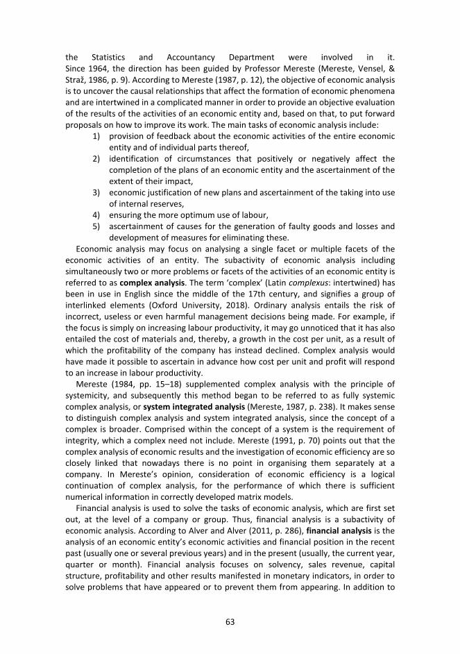
63

the Statistics and Accountancy Department were involved in it. Since 1964, the direction has been guided by Professor Mereste (Mereste, Vensel, & Straž, 1986, p. 9). According to Mereste (1987, p. 12), the objective of economic analysis is to uncover the causal relationships that affect the formation of economic phenomena and are intertwined in a complicated manner in order to provide an objective evaluation of the results of the activities of an economic entity and, based on that, to put forward proposals on how to improve its work. The main tasks of economic analysis include:

1) provision of feedback about the economic activities of the entire economicentity and of individual parts thereof,

2) identification of circumstances that positively or negatively affect thecompletion of the plans of an economic entity and the ascertainment of theextent of their impact,

3) economic justification of new plans and ascertainment of the taking into useof internal reserves,

4) ensuring the more optimum use of labour,5) ascertainment of causes for the generation of faulty goods and losses and

development of measures for eliminating these.Economic analysis may focus on analysing a single facet or multiple facets of the

economic activities of an entity. The subactivity of economic analysis including simultaneously two or more problems or facets of the activities of an economic entity is referred to as complex analysis. The term ‘complex’ (Latin complexus: intertwined) has been in use in English since the middle of the 17th century, and signifies a group of interlinked elements (Oxford University, 2018). Ordinary analysis entails the risk of incorrect, useless or even harmful management decisions being made. For example, if the focus is simply on increasing labour productivity, it may go unnoticed that it has also entailed the cost of materials and, thereby, a growth in the cost per unit, as a result of which the profitability of the company has instead declined. Complex analysis would have made it possible to ascertain in advance how cost per unit and profit will respond to an increase in labour productivity.

Mereste (1984, pp. 15–18) supplemented complex analysis with the principle of systemicity, and subsequently this method began to be referred to as fully systemic complex analysis, or system integrated analysis (Mereste, 1987, p. 238). It makes sense to distinguish complex analysis and system integrated analysis, since the concept of a complex is broader. Comprised within the concept of a system is the requirement of integrity, which a complex need not include. Mereste (1991, p. 70) points out that the complex analysis of economic results and the investigation of economic efficiency are so closely linked that nowadays there is no point in organising them separately at a company. In Mereste’s opinion, consideration of economic efficiency is a logical continuation of complex analysis, for the performance of which there is sufficient numerical information in correctly developed matrix models.

Financial analysis is used to solve the tasks of economic analysis, which are first set out, at the level of a company or group. Thus, financial analysis is a subactivity of economic analysis. According to Alver and Alver (2011, p. 286), financial analysis is the analysis of an economic entity’s economic activities and financial position in the recent past (usually one or several previous years) and in the present (usually, the current year, quarter or month). Financial analysis focuses on solvency, sales revenue, capital structure, profitability and other results manifested in monetary indicators, in order to solve problems that have appeared or to prevent them from appearing. In addition to

64

other research methods, both complex and system integrated analysis could be used when financial analysis is performed (see Figure 1.5 for illustration).

Financial statement analysis is a subactivity of financial analysis, the objective of which is to assess the functioning and financial position of an economic entity based on financial statements (Alver & Alver, 2011, p. 287). This results in the provision of current and future investors, management, creditors, employees and other interested parties with the information required for decision-making. In many countries, the annual reports of companies are publicly available; however, evaluation of the balance sheet total, sales revenue and profit alone are not sufficient for making substantiated management decisions. The more detailed use of information provided in the balance sheet, income statement and cash flow statement makes it possible to assess the level of development of the company, along with its profitability, solvency, efficiency of the use of its assets and labour, the structure of its assets and the sources of financing, earnings quality, etc. The latter is precisely the focus of this doctoral thesis: in chapter 2, the author is applying data from financial statements when further developing the usage of the efficiency matrix and its developments.

The most important conclusions from the first chapter are, as follows: − Efficiency is a multidimensional phenomenon. To analyse this, a number of

analytical models have been created since the 1920s. − The main advantages of the efficiency matrix concept developed in this thesis

are its systemicity. That is, the ability to involve various facets of business activities in a single model), workability with a small quantity of initial data and the options for developing the model further (analysis in terms of components that have an impact on efficiency; calculation of both static and dynamic overall efficiency indices.

− Empirical, deductive and inductive approaches are used to classify financial ratios but the only consensus relates to the most commonly used ratio categories like profitability and liquidity. Other ratio categories differed across studies. Factor analysis is mainly used to classify ratios using statistical methods. The removal of outliers is important when using statistical methods in financial ratio analysis.

− Liquidity, solvency, efficiency of assets usage, investment profitability and assets structure are well covered by most popular and well-known financial ratios. Sales profitability, efficiency of labour usage, cost efficiency and earnings quality are the main examples of business aspects poorly covered by popular financial ratios.

To summarise, it has to be noted that, despite many analysis models, today there remains a clear need for the measurement of economic efficiency and for an economic model that characterises change, the development of which is indeed addressed in the next chapter.

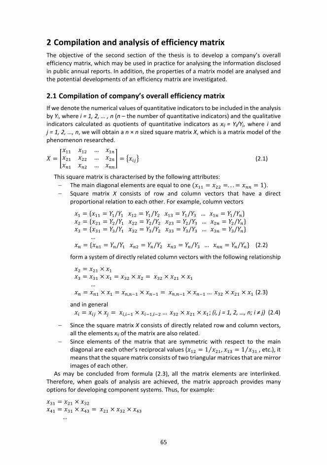
65

2 Compilation and analysis of efficiency matrix The objective of the second section of the thesis is to develop a company’s overall efficiency matrix, which may be used in practice for analysing the information disclosed in public annual reports. In addition, the properties of a matrix model are analysed and the potential developments of an efficiency matrix are investigated.

2.1 Compilation of company’s overall efficiency matrix If we denote the numerical values of quantitative indicators to be included in the analysis by Yi, where i = 1, 2, … , n (n – the number of quantitative indicators) and the qualitative indicators calculated as quotients of quantitative indicators as xij = Yi/Yj, where i and j = 1, 2, …, n, we will obtain a n × n sized square matrix X, which is a matrix model of the phenomenon researched.

𝑋𝑋 = �𝑥𝑥11 𝑥𝑥12 … 𝑥𝑥1𝑛𝑛𝑥𝑥21 𝑥𝑥22 … 𝑥𝑥2𝑛𝑛𝑥𝑥𝑛𝑛1 𝑥𝑥𝑛𝑛2 … 𝑥𝑥𝑛𝑛𝑛𝑛

� = �𝑥𝑥𝑝𝑝𝑖𝑖� (2.1)

This square matrix is characterised by the following attributes: − The main diagonal elements are equal to one (𝑥𝑥11 = 𝑥𝑥22 =. . . = 𝑥𝑥𝑛𝑛𝑛𝑛 = 1). − Square matrix X consists of row and column vectors that have a direct

proportional relation to each other. For example, column vectors

𝑥𝑥1 = {𝑥𝑥11 = 𝑌𝑌1/𝑌𝑌1 𝑥𝑥12 = 𝑌𝑌1/𝑌𝑌2 𝑥𝑥13 = 𝑌𝑌1/𝑌𝑌3 … 𝑥𝑥1𝑛𝑛 = 𝑌𝑌1/𝑌𝑌𝑛𝑛}. 𝑥𝑥2 = {𝑥𝑥21 = 𝑌𝑌2/𝑌𝑌1 𝑥𝑥22 = 𝑌𝑌2/𝑌𝑌2 𝑥𝑥23 = 𝑌𝑌2/𝑌𝑌3 … 𝑥𝑥2𝑛𝑛 = 𝑌𝑌2/𝑌𝑌𝑛𝑛} 𝑥𝑥3 = {𝑥𝑥31 = 𝑌𝑌3/𝑌𝑌1 𝑥𝑥32 = 𝑌𝑌3/𝑌𝑌2 𝑥𝑥33 = 𝑌𝑌3/𝑌𝑌3 … 𝑥𝑥3𝑛𝑛 = 𝑌𝑌3/𝑌𝑌𝑛𝑛}

… 𝑥𝑥𝑛𝑛 = {𝑥𝑥𝑛𝑛1 = 𝑌𝑌𝑛𝑛/𝑌𝑌1 𝑥𝑥𝑛𝑛2 = 𝑌𝑌𝑛𝑛/𝑌𝑌2 𝑥𝑥𝑛𝑛3 = 𝑌𝑌𝑛𝑛/𝑌𝑌3 … 𝑥𝑥𝑛𝑛𝑛𝑛 = 𝑌𝑌𝑛𝑛/𝑌𝑌𝑛𝑛} (2.2)

form a system of directly related column vectors with the following relationship

𝑥𝑥2 = 𝑥𝑥21 × 𝑥𝑥1 𝑥𝑥3 = 𝑥𝑥31 × 𝑥𝑥1 = 𝑥𝑥32 × 𝑥𝑥2 = 𝑥𝑥32 × 𝑥𝑥21 × 𝑥𝑥1 … 𝑥𝑥𝑛𝑛 = 𝑥𝑥𝑛𝑛1 × 𝑥𝑥1 = 𝑥𝑥𝑛𝑛,𝑛𝑛−1 × 𝑥𝑥𝑛𝑛−1 = 𝑥𝑥𝑛𝑛,𝑛𝑛−1 × 𝑥𝑥𝑛𝑛−1 … 𝑥𝑥32 × 𝑥𝑥21 × 𝑥𝑥1 (2.3)

and in general 𝑥𝑥𝑝𝑝 = 𝑥𝑥𝑝𝑝𝑖𝑖 × 𝑥𝑥𝑖𝑖 = 𝑥𝑥𝑝𝑝,𝑝𝑝−1 × 𝑥𝑥𝑝𝑝−1,𝑝𝑝−2 … 𝑥𝑥32 × 𝑥𝑥21 × 𝑥𝑥1; (i, j = 1, 2, …, n; i ≠ j) (2.4)

− Since the square matrix X consists of directly related row and column vectors, all the elements xij of the matrix are also related.

− Since elements of the matrix that are symmetric with respect to the main diagonal are each other’s reciprocal values (𝑥𝑥12 = 1 𝑥𝑥21⁄ , 𝑥𝑥13 = 1 𝑥𝑥31 ⁄ , etc.), it means that the square matrix consists of two triangular matrices that are mirror images of each other.

As may be concluded from formula (2.3), all the matrix elements are interlinked. Therefore, when goals of analysis are achieved, the matrix approach provides many options for developing component systems. Thus, for example:

𝑥𝑥31 = 𝑥𝑥21 × 𝑥𝑥32 𝑥𝑥41 = 𝑥𝑥31 × 𝑥𝑥43 = 𝑥𝑥21 × 𝑥𝑥32 × 𝑥𝑥43

…

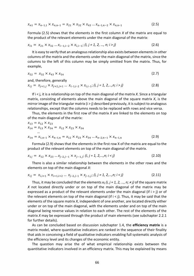
66

𝑥𝑥𝑛𝑛1 = 𝑥𝑥𝑛𝑛–1,1 × 𝑥𝑥𝑛𝑛,𝑛𝑛–1 = 𝑥𝑥21 × 𝑥𝑥32 × 𝑥𝑥43 … 𝑥𝑥𝑛𝑛–1,𝑛𝑛−2 × 𝑥𝑥𝑛𝑛,𝑛𝑛–1 (2.5)

Formula (2.5) shows that the elements in the first column X of the matrix are equal to the product of the relevant elements under the main diagonal of the matrix:

𝑥𝑥𝑝𝑝1 = 𝑥𝑥21 × 𝑥𝑥32 … 𝑥𝑥𝑝𝑝−1,𝑝𝑝−2 × 𝑥𝑥𝑝𝑝,𝑝𝑝−1; (i, j = 1, 2, …, n; i > j) (2.6)

It is easy to verify that an analogous relationship also exists between elements in other columns of the matrix and the elements under the main diagonal of the matrix, since the columns to the left of this column may be simply omitted from the matrix. Thus, for example,

𝑥𝑥52 = 𝑥𝑥32 × 𝑥𝑥43 × 𝑥𝑥54 (2.7)

and, therefore, generally 𝑥𝑥𝑝𝑝𝑖𝑖 = 𝑥𝑥𝑖𝑖+1,𝑖𝑖 × 𝑥𝑥𝑖𝑖+2,𝑖𝑖+1 … 𝑥𝑥𝑝𝑝–1,𝑝𝑝–2 × 𝑥𝑥𝑝𝑝,𝑝𝑝–1; (i, j = 1, 2,…,n; i > j) (2.8)

If i < j, it is a relationship on top of the main diagonal of the matrix X. Since a triangular matrix, consisting of elements above the main diagonal of the square matrix X, is the mirror image of the triangular matrix (i > j) described previously, it is subject to analogous relationships, except that the columns needs to be replaced with rows and vice versa.

Thus, the elements in the first row of the matrix X are linked to the elements on top of the main diagonal of the matrix: 𝑥𝑥13 = 𝑥𝑥12 × 𝑥𝑥23 𝑥𝑥14 = 𝑥𝑥13 × 𝑥𝑥34 = 𝑥𝑥12 × 𝑥𝑥23 × 𝑥𝑥34 … 𝑥𝑥1𝑛𝑛 = 𝑥𝑥1,𝑛𝑛–1 × 𝑥𝑥𝑛𝑛–1,𝑛𝑛 = 𝑥𝑥12 × 𝑥𝑥23 × 𝑥𝑥34 … 𝑥𝑥𝑛𝑛–2,𝑛𝑛−1 × 𝑥𝑥𝑛𝑛–1,𝑛𝑛 (2.9)

Formula (2.9) shows that the elements in the first row X of the matrix are equal to the product of the relevant elements on top of the main diagonal of the matrix.

𝑥𝑥1𝑖𝑖 = 𝑥𝑥12 × 𝑥𝑥23 … 𝑥𝑥𝑖𝑖–2,𝑖𝑖−1 × 𝑥𝑥𝑖𝑖−1,𝑖𝑖; (i, j = 1, 2,…,n; i < j) (2.10)

There is also a similar relationship between the elements in the other rows and the elements on top of the main diagonal X:

𝑥𝑥𝑝𝑝𝑖𝑖 = 𝑥𝑥𝑝𝑝,𝑝𝑝+1 × 𝑥𝑥𝑝𝑝+1,𝑝𝑝+2 … 𝑥𝑥𝑖𝑖–2,𝑖𝑖–1 × 𝑥𝑥𝑖𝑖–1,𝑖𝑖; (i, j = 1, 2,…,n; i < j) (2.11)

Thus, it may be concluded that the elements xij (i, j = 1, 2, …, n; ≠ j) of the square matrix X not located directly under or on top of the main diagonal of the matrix may be expressed as a product of the relevant elements under the main diagonal (if i > j) or of the relevant elements on top of the main diagonal (if i < j). Thus, it may be said that the elements of the square matrix X, independent of one another, are located directly either under or on top of the main diagonal, with the elements under and on top of the main diagonal being reverse values in relation to each other. The rest of the elements of the matrix X may be expressed through the product of main elements (see subchapter 2.2.1 for further details).

As can be concluded based on discussion subchapter 1.4, the efficiency matrix is a matrix model, where quantitative indicators are ranked in the sequence of their finality that aids in conceiving a field of qualitative indicators enabling full systematic analysis of the efficiency level and its changes of the economic entity.

The question may arise the of what empirical relationship exists between the quantitative indicators involved in an efficiency matrix. This may be explained by means

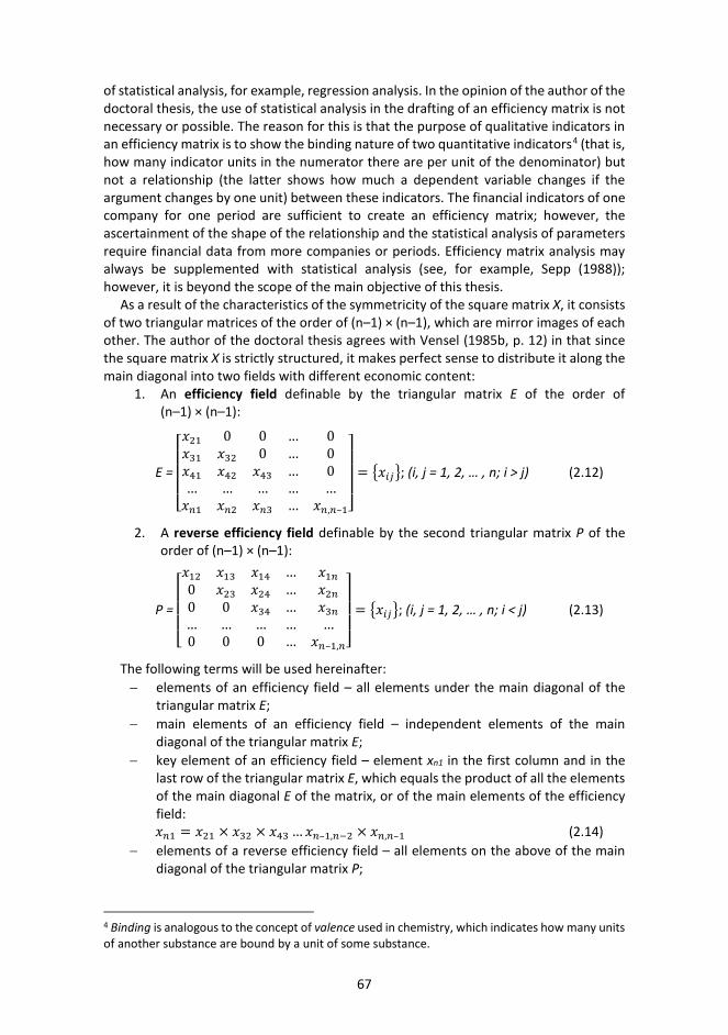
67

of statistical analysis, for example, regression analysis. In the opinion of the author of the doctoral thesis, the use of statistical analysis in the drafting of an efficiency matrix is not necessary or possible. The reason for this is that the purpose of qualitative indicators in an efficiency matrix is to show the binding nature of two quantitative indicators4 (that is, how many indicator units in the numerator there are per unit of the denominator) but not a relationship (the latter shows how much a dependent variable changes if the argument changes by one unit) between these indicators. The financial indicators of one company for one period are sufficient to create an efficiency matrix; however, the ascertainment of the shape of the relationship and the statistical analysis of parameters require financial data from more companies or periods. Efficiency matrix analysis may always be supplemented with statistical analysis (see, for example, Sepp (1988)); however, it is beyond the scope of the main objective of this thesis.

As a result of the characteristics of the symmetricity of the square matrix X, it consists of two triangular matrices of the order of (n–1) × (n–1), which are mirror images of each other. The author of the doctoral thesis agrees with Vensel (1985b, p. 12) in that since the square matrix X is strictly structured, it makes perfect sense to distribute it along the main diagonal into two fields with different economic content:

1. An efficiency field definable by the triangular matrix E of the order of(n–1) × (n–1):

E =

⎣⎢⎢⎢⎡𝑥𝑥21 0 0 … 0𝑥𝑥31 𝑥𝑥32 0 … 0𝑥𝑥41 𝑥𝑥42 𝑥𝑥43 … 0… … … … …𝑥𝑥𝑛𝑛1 𝑥𝑥𝑛𝑛2 𝑥𝑥𝑛𝑛3 … 𝑥𝑥𝑛𝑛,𝑛𝑛–1⎦

⎥⎥⎥⎤

= �𝑥𝑥𝑝𝑝𝑖𝑖�; (i, j = 1, 2, … , n; i > j) (2.12)

2. A reverse efficiency field definable by the second triangular matrix P of theorder of (n–1) × (n–1):

P =

⎣⎢⎢⎢⎡𝑥𝑥12 𝑥𝑥13 𝑥𝑥14 … 𝑥𝑥1𝑛𝑛0 𝑥𝑥23 𝑥𝑥24 … 𝑥𝑥2𝑛𝑛0 0 𝑥𝑥34 … 𝑥𝑥3𝑛𝑛… … … … …0 0 0 … 𝑥𝑥𝑛𝑛–1,𝑛𝑛⎦

⎥⎥⎥⎤

= �𝑥𝑥𝑝𝑝𝑖𝑖�; (i, j = 1, 2, … , n; i < j) (2.13)

The following terms will be used hereinafter: − elements of an efficiency field – all elements under the main diagonal of the

triangular matrix E; − main elements of an efficiency field – independent elements of the main

diagonal of the triangular matrix E; − key element of an efficiency field – element xn1 in the first column and in the

last row of the triangular matrix E, which equals the product of all the elements of the main diagonal E of the matrix, or of the main elements of the efficiency field: 𝑥𝑥𝑛𝑛1 = 𝑥𝑥21 × 𝑥𝑥32 × 𝑥𝑥43 … 𝑥𝑥𝑛𝑛–1,𝑛𝑛−2 × 𝑥𝑥𝑛𝑛,𝑛𝑛–1 (2.14)

− elements of a reverse efficiency field – all elements on the above of the main diagonal of the triangular matrix P;

4 Binding is analogous to the concept of valence used in chemistry, which indicates how many units of another substance are bound by a unit of some substance.

68

− main elements of a reverse efficiency field – independent elements of the main diagonal of the triangular matrix P;

− key element of a reverse efficiency field – element x1n in the first row and in the last column of a triangular matrix P, which equals the product of all the elements of the main diagonal P of the matrix, or product of all the main elements of the reverse efficiency field: 𝑥𝑥1𝑛𝑛 = 𝑥𝑥12 × 𝑥𝑥23 × 𝑥𝑥34 … 𝑥𝑥𝑛𝑛–2,𝑛𝑛−1 × 𝑥𝑥𝑛𝑛–1,𝑛𝑛 (2.15)

Naturally, the key element x1n of a reverse efficiency field is the reverse value of the key element xn1 of an efficiency field.

Of significance for drafting an efficiency matrix are the choice and sequence of quantitative financial indicators included in the matrix. The selection of initial quantitative indicators depends on the purpose of the analysis. One can analyse the business performance of a company as a whole or some more specific aspect such as profitability, solvency, utilisation of labour or fixed assets, etc.

Due to the symmetry of the square matrix, the focus of analysis will mostly be on investigating and analysing the relationships between the elements of triangular matrix E; however, matrix P representing the reverse efficiency field should also be included in the efficiency analysis.

According to Luur (1982, pp. 134–136), the quantitative indicators used for constructing the efficiency matrix are divided into output and input indicators; therefore, the efficiency field can be divided into three areas 5 (Figure 2.1):

− Triangular output matrix (OM) that characterises the efficiency of the final result of economic activities. Its elements are financial ratios characterising the proportions between the output indicators, which are also called coordination ratios.

− Triangular input matrix (IM) that characterise resources used. Its elements are financial ratios characterising the proportions between the input indicators, which are also classified as coordination ratios.

− Quadrilateral input-output matrix (IOM), where the elements are all the other financial ratios showing the relationships between input and output indicators (for example, income and resource ratios), which are classified as intensity ratios.

5 These submatrices must not be mistaken for Leontief’s input-output models, where matrix field elements are variables subject to being added up.

69

Figure 2.1. Division of efficiency field into three submatrices. Source: (Луур, 1982, pp. 134–136).

In developing an efficiency matrix, Vensel (1985b, pp. 15–16) classifies the quantitative indicators used into four groups, one of which characterises output indicators and three characterise input indicators:

− indicators characterising the manufacturing process (for example, quantity of goods, sales revenue, costs of goods sold, gross profit, etc.),

− indicators reflecting the use of labour (for example, number of employees, labour expenses, training expenses, etc.),

− indicators reflecting the use of tangible fixed assets (for example, acquisition costs of tangible fixed assets, investments in non-current assets, etc.),

− indicators reflecting the use of current assets and materials (for example, cost of inventories, quantity and cost of materials used, etc.).

Alver (1988, pp. 247–248) considers that expenses and resources as input indicators need to be distinguished. Resources are always linked to a certain moment in time (for example, the beginning or end of a month, quarter or year), and thus a moment series may be formed out of numerical data characterising resources. Expenses, by contrast, are always linked to a period of time, and a period series may be formed out of the indicators characterising them. Thus, expenses are the targeted consumption of resources and are therefore closer to output indicators than resources. Alver (1989) suggests a more precise principle for arranging the quantitative parameters: resources are metamorphosed via expenses into the final result. This means that input indicators are split into resource and expense indicators. Therefore, it is possible to use the following formula for the arranging:

RESOURCES EXPENSES RESULTS

As a result, an efficiency field may be divided into six submatrices (Figure 2.2): − Triangular output (results) matrix (OM) that characterises the efficiency of the

final results of economic activities. Its elements are financial ratios characterising the proportions between the output indicators.

− Triangular input matrix (RM) that characterise usage of resources for economic activities. Its elements are financial ratios characterising the proportions between the input indicators, which are also classified as coordination ratios.

70

− Triangular expense matrix (EM) that characterise expenses made. Its elements are financial ratios characterising the proportions between the expense indicators.

− Quadrilateral expense-output matrix (EOM), where all elements are financial ratios showing the relationships between output and expense indicators.

− Quadrilateral resource-expense matrix (REM), where all elements are financial ratios showing the relationships between expense and resource indicators.

- Quadrilateral resource-output matrix (ROM), where the elements are all the financial ratios showing the relationships between output and resource indicators, which are classified as intensity ratios.

As in the case of the division of quantitative indicators into three groups, in the case of a division six ways there are also coordination ratios characterising the relationships of the same group of indicators in triangular matrices and intensity ratios between various indicator groups in quadrilateral matrices.

Figure 2.2. Division of efficiency field into six submatrices. Source: (Alver J. , 1988, p. 251).

The business activities of a company consist of its operating activities, investment activities and financing activities. Time-wise, investment activities occur first (for example, the shareholder makes an owners’ equity contribution, the company receives a loan from a bank or other financial institution, etc.). After finding sources for financing, a company can begin investment activities (for example, acquire a new tangible item of non-current assets). Next up are the operating activities, or the earning of current income and cash inflows. The latter also entails running costs and cash outflows. All this information is available from public annual reports.

In the opinion of the author of the doctoral thesis, in order to reflect the integrity of the business activities of a company, it makes sense to supplement groups of quantitative indicators in an efficiency matrix as follows:

− include a group that characterises the financing of a company or its use of capital,

− split the group of result indicators into three: − income indicators that characterise a company’s ability to earn sales

and other operating income,

71

− profit indicators that show the ability to earn a profit, − cash flow indicators showing whether a company is earning money in

addition to profit. Thus, raising capital makes it possible to invest in resources that, through expenses,

are transformed into income, profit and cash flow:

CAPITAL RESOURCES EXPENSES INCOME PROFIT CASH FLOW

The sources of financing for a company may be divided into: 1) Capital:

a. owners’ equity,b. financial liabilities (loan capital),

2) Other sources of financing (for example, payables and provisions).A dividend has to be paid for the use of owners’ equity and interest for loan capital.

As a rule, other sources of financing are free of charge if payments are made in time, which means that these are the cheapest sources of financing for a company. The main advantage of including a group that characterises capital indicators is that it makes it possible to analyse return on capital and financial leverage.

Resources may be classified as follows: 1) Assets. The future economic benefit embodied in an asset is the potential to

contribute, directly or indirectly, to the flow of cash and cash equivalents to theentity (International Accounting Standards Board, 2010). Assets are split into non-current and current assets.

a. Non-current assets concerning which a company is required to disclose,as a rule, how they are divided between the tangible and intangible non-current assets used in its everyday business activities and the financialand real estate investments. As a rule, it is further determined how eachgroup of non-current assets breaks down by type. For example, in thecase of tangible non-current assets their breakdown into land, buildings, machinery and equipment and other inventory is disclosed both at bookand current value. Internally at a company, in addition, the cost and thecarrying value of a specific item of non-current assets, in what businessor manufacturing process it is used and for how many hours are knownprecisely.

b. Current assets are divided into cash, short-term financial investments,receivables and inventories. Also in the case of current assets, as a rulethe notes to the annual reports specify their more detailed breakdownfor every group. For example, inventories are divided into directmaterials and other materials, work-in-progress, finished goods andgoods purchased for resale. At the same time, more detailed information is known at a company about the quantity of every item of inventories,how much and what kind of material is needed to make a certainproduct, etc.

2) Number of employees. As a rule, annual reports disclose the average number ofemployees in full-time equivalents (FTEs). At a company, in addition, the numberof employees by department and business segment is known.

The definition of expenses encompasses losses as well as those expenses that arise in the course of the ordinary activities of the entity (International Accounting Standards Board, 2010). Expenses are grouped by type or function in an income statement. When

72

expenses are grouped by type, the cost of goods and services bought in, various operating expenses – labour expenses, depreciation and other operating expenses – are presented. Function-based grouping specifies the costs of the goods and services sold, marketing expenses, general and administrative expenses and other operating expenses. In addition to that, a company may incur financial expenses and income tax expenses. Annual reports are prepared according to international standards, which additionally specify operating expenses in terms of main business segments.

The definition of income encompasses both revenue and gains (International Accounting Standards Board, 2010). Revenue arises in the course of the ordinary activities of an entity and is referred to by a variety of different names including sales, fees, interest, dividends, royalties and rent. Gains represent other items that meet the definition of income and may, or may not, arise in the course of the ordinary activities of an entity. Gains include, for example, those arising on the disposal of non-current assets. The definition of income also includes unrealised gains; for example, those arising on the revaluation of marketable securities.

Profit is spit as the difference between income and expenses. Depending on the kinds of income and expenses involved in the calculation, gross profit, EBITDA, operating profit, earnings before taxes and net profit are distinguished in annual reports.

Cash flow is divided into three in the cash flow statement: operating, investment and financing cash flows. The net operating cash flow may be compared to the operating profit specified in the income statement of the company. For both investors and creditors, it is important to know whether a company is earning money (not just operating profit) from its operating activities as it is cash position that largely determines how a company will fare going forward. When cash flows earned from the operating activities and the investing cash flows are added up, free cash is obtained, which characterises the ability of the company to meet its creditors’ and investors’ need for cash.

The breakdown of quantitative indicators according to Luur (1982) and Alver (1989) along with the vision of the author of the thesis is depicted in Figure 2.3.

Figure 2.3. Classification of quantitative indicators. Source: (by the author).

Accordingly, to achieve a more comprehensive analysis result, it makes sense to divide an efficiency field into 21 submatrices, six of which are triangular matrices and 15 quadrilateral matrices (Figure 2.4). Triangular matrices characterise proportions between the various parts of one group of quantitative indicators:

73

− Elements of cash flow matrix (CM) are financial ratios characterising the proportions between the cash flow indicators. Net operating cash flow, free cash flow and total net cash flow can be deployed as output indicators. In addition, free cash flow can be split into free cash flow to the company and free cash flow to equity.

− Elements of profit matrix (PM) are financial ratios characterising the proportions between the profit indicators. Gross profit, earnings before interests and taxes, depreciation and amortisation (EBITDA), operating profit, earnings before taxes (EBT) and net profit are commonly used profit indicators. As the companies can have different capital structures, the author advises using earnings before interests and taxes (EBIT = EBT + Interest expense = Net profit + Taxes + Interest expense) as a profit indicator when there is a need to ensure comparability between companies using different sources of financing. In addition, depending on the industry analysed, earnings before interests and taxes, depreciation and amortisation and rent expenses (EBITDAR), earnings before interests and taxes, depreciation and amortisation, rent and management fees (EBITDARM), net operating profit after tax (NOPAT) and economic value added (EVA = operating profit + labour expenses + depreciation and amortisation) can be deployed. The advantage of EVA is that in addition to investors it takes into account the contribution of creditors, employees, suppliers and government (Alver & Alver, 2011, p. 152).

− Elements of income matrix (IM) are financial ratios characterising the proportions between the income indicators. Sales revenue (net sales) should mainly be used as an income indicator. When relevant, total operating income (sales revenue + other income) or total income (total operating income + financial income (e.g. interest, dividends)) could also be utilised.

− Elements of expense matrix (EM) are financial ratios characterising the proportions between the expense indicators. Depending on the layout of the income statement used by a company, type- or function-based grouping of expenses may be used. When different companies are compared, it makes sense to use either total operating expenses or total expenses (total operating expenses + financial expenses + income tax expense), since the value of either indicator does not depend on the layout of the preparation of the income statement. At the time of preparation of this thesis, companies operating in Estonia are required to disclose the total amount of labour expenses regardless of the layout selected for the income statement.

− Elements of resource matrix (RM) are financial ratios characterising the proportions between the resource indicators. The resources of a company consist of labour and assets generating an economic benefit, whose value is disclosed on the balance sheet. For the selection of quantitative indicators, both total assets and parts thereof (current assets, non-current assets and elements thereof) may be used.

− Elements of capital matrix (KM) are financial ratios characterising the proportions between the capital indicators. From publicly available annual reports, information may be initially obtained about capital invested, owners’ equity and loan capital. To ensure comparability between companies, it is advisable also to use total capital (= owners’ equity + loan capital) in an efficiency matrix.

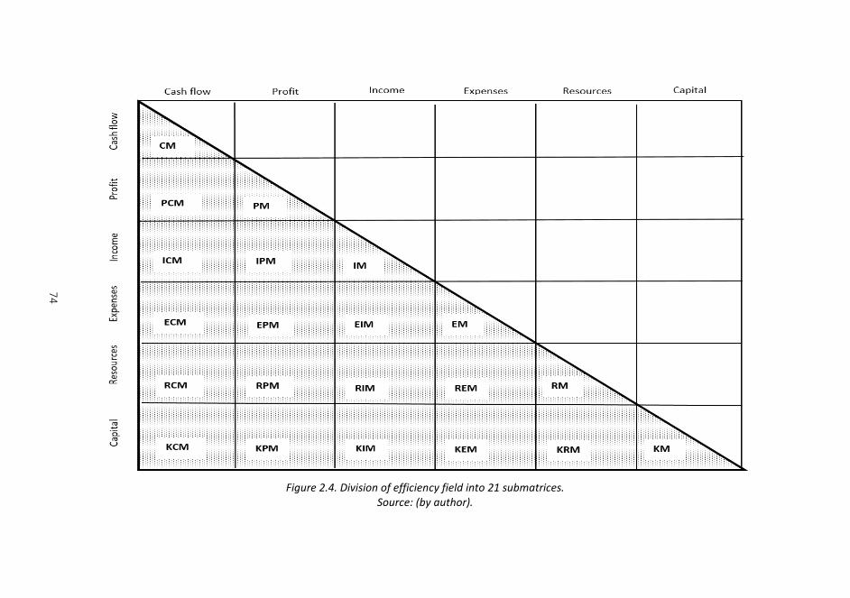
74

Figure 2.4. Division of efficiency field into 21 submatrices. Source: (by author).

75

Quadrilateral matrices characterise proportions between various parts of two groups of quantitative indicators. Designations of quadrilateral matrices have been developed in order of finality: a group of elements ahead in terms of its level of finality is presented first. The first three quadrilateral matrices characterise mutual proportions between output indicators:

− Elements of profit-cash flow matrix (PCM) are financial ratios characterising the proportions between the cash flow and profit indicators. These ratios show whether, in addition to profit, a company is also earning money, or, in the case of a loss, this also entails a financial expenditure. The more money a company is earning per euro of profit earned, the more efficient it is. In the case of ratios marked as negative in this submatrix, it is necessary to investigate further the reason why the profit and cash flow indicators analysed are marked differently. This may happen if a company is earning a profit, yet its net cash flow is negative due to the long payment terms provided for its clients, its customers’ poor solvency and/or high investment expenditures at the company analysed. However, the opposite may be the case as well: despite a loss, the net cash flow of a company is positive, since prepayments are received from clients or payments are received for sales revenue earned in previous periods.

− Elements of income-cash flow matrix (ICM) are financial ratios characterising the proportions between the cash flow and income indicators. These ratios show how many cents of net cash flow a company is earning per euro of income. The more net cash flow a company is earning per euro of sales revenue, the more efficient it is. Since income indicators are positively marked, ratios with negative values in this submatrix mean that the net cash flow of the company is negative. In this case, the analyst should investigate why the expenditures of the company exceed its receipts.

− Elements of income-profit matrix (IPM) are financial ratios characterising the proportions between the profit and income indicators. The ratios in this submatrix show the profitability of the sales of a company and one finds out how many cents of profit the company is earning per euro of income. The more profit a company is earning per euro earned as income, the more efficient it is. Since income indicators are positively marked, ratios with negative values in this submatrix mean how many cents of loss the company is earning per euro of income.

The next nine quadrilateral matrices characterise mutual relationships between input and output indicators:

− Elements of expense-cash flow matrix (ECM) are financial ratios characterising the proportions between the cash flow and expense indicators. First, it is important to consider that whereas today an income statement often presents expenses with a minus sign, an efficiency matrix shows expenses in their absolute value, or with a plus sign. The values of the ratios in this submatrix show how much money a company is earning per euro of expenses. The more money a company is earning per euro spent, the more efficient it is. Since expense indicators are positively marked, ratios with negative values in this submatrix mean that the net cash flow of the company is negative.

− Elements of resource-cash flow matrix (RCM) are financial ratios characterising the proportions between the cash flow and resource indicators. These ratios show how many cents of net cash flow a company is earning on either per euro

76

invested in assets or per employee. The more money a company is earning per euro invested in assets and per employee, the more efficient it is. Since resource indicators are positively marked, ratios with negative values in this submatrix mean that the net cash flow analysed is negative and the analyst needs to delve into the reasons for it.

− Elements of capital-cash flow matrix (KCM) are financial ratios characterising the proportions between the cash flow and capital indicators. The ratios in this submatrix show how many cents of net cash flow a company is earning per euro of owners’ equity and loan capital raised. The more money a company is earning per euro of capital raised, the more efficient the company is. Since capital indicators are positively marked, ratios with negative values in this submatrix mean that the net cash flow analysed is negative.

− Elements of expense-profit matrix (EPM) are financial ratios characterising the proportions between the profit and expense indicators. The ratios in this submatrix show the cost-efficiency of a company and one finds out how many cents of profit the company is earning per euro spent. The more profit a company is earning per euro spent, the more efficient it is. Since expense indicators are presented in their absolute value, ratios with negative values mean that the profit indicator in the numerator of the ratio is negative.

− Elements of resource-profit matrix (RPM) are financial ratios characterising the proportions between the profit and resource indicators. These ratios show how many cents of profit a company is earning per euro invested in assets or per employee. The more profit a company is earning per euro invested in assets and per employee, the more efficient it is. Since resource indicators are positively marked, ratios with negative values in this submatrix mean that the profit indicator analysed is negative.

− Elements of capital-profit matrix (KPM) are financial ratios characterising the proportions between the profit and capital indicators. The ratios in this submatrix show return on investment, that is, how many cents of profit the company is earning per euro raised as owners’ equity and loan capital. The more profit a company is earning per euro raised as capital, the more efficient it is. Since capital indicators are positively marked, ratios with negative values in this submatrix indicate that the profit indicator analysed is negative.

− Elements of expense-income matrix (EIM) are financial ratios characterising the proportions between the income and expense indicators. The ratios in this submatrix show how much income a company has been able to earn per euro spent. The higher the ratio between income and expenses is, the more efficient it is.

− Elements of resource-income matrix (RIM) are financial ratios characterising the proportions between the income and resource indicators. These ratios show how much income a company is earning per euro invested in assets or per employee. The more income a company is earning per euro invested in assets and per employee, the more efficient it is.

− Elements of capital-income matrix (KIM) are financial ratios characterising the proportions between the income and capital indicators. The ratios in this submatrix show how much income a company is earning per euro of owners’ equity and loan capital raised. The more income a company is earning per euro raised as capital, the more efficient it is.

77

The last three submatrices characterise the mutual proportions of input indicators: − Elements of resource-expense matrix (REM) are financial ratios characterising

the proportions between the expense and resource indicators. These ratios show how many euros a company is spending per euro invested in assets or per employee. In the case of reasonable business activities, expenses are generated in the process of targeted consumption. Thus, the higher the ratio between expenses and resources, the greater the intensity with which the company is operating and the more efficient it is.

− Elements of capital-expense matrix (KEM) are financial ratios characterising the proportions between the expense and capital indicators. The ratios in this submatrix show how many euros a company is spending per euro of owners’ equity and loan capital raised. The higher the ratio between expenses and capital raised, the greater the intensity with which the company is operating and the more efficient it is.

− Elements of capital-resource matrix (KRM) are financial ratios characterising the proportions between the resource and capital indicators. The ratios in this submatrix show how much a company has invested in assets per euro raised as capital or per employee. The higher the ratio between resource and capital indicators, the more efficient the company is.

All 21 submatrices appear in a single efficiency matrix only if all six groups of quantitative indicators are involved and at least two indicators from every group are represented. If one indicator is involved from a group of quantitative indicators, no triangular matrices characterising the proportions of the relevant group are formed.

A summary (but by no means final) list of quantitative indicators, available from annual reports, to be involved in an efficiency matrix is set out by group in Table 2.1. IFRS Taxonomy 2018 (International Accounting Standards Board, 2018) has been used as the basis for the list of quantitative indicators. For the resources and capital groups, the author of doctoral thesis strongly advises using period average values (e.g. annual average) to ensure better comparability of expense, income, profit and cash flow indicators that already have periodic values in financial statements. The analyst can choose the relevant items from each group according to his/her research goal.

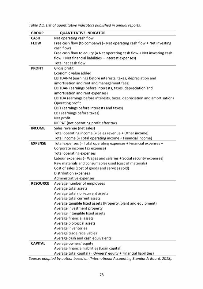
78

Table 2.1. List of quantitative indicators published in annual reports.

GROUP QUANTITATIVE INDICATOR CASH FLOW

Net operating cash flow Free cash flow (to company) (= Net operating cash flow + Net investing cash flow) Free cash flow to equity (= Net operating cash flow + Net investing cash flow + Net financial liabilities – Interest expenses) Total net cash flow

PROFIT Gross profit Economic value added EBITDARM (earnings before interests, taxes, depreciation and amortisation and rent and management fees) EBITDAR (earnings before interests, taxes, depreciation and amortisation and rent expenses) EBITDA (earnings before interests, taxes, depreciation and amortisation) Operating profit EBIT (earnings before interests and taxes) EBT (earnings before taxes) Net profit NOPAT (net operating profit after tax)

INCOME Sales revenue (net sales) Total operating income (= Sales revenue + Other income) Total income (= Total operating income + Financial income)

EXPENSE Total expenses (= Total operating expenses + Financial expenses + Corporate income tax expense) Total operating expenses Labour expenses (= Wages and salaries + Social security expenses) Raw materials and consumables used (cost of materials) Cost of sales (cost of goods and services sold) Distribution expenses Administrative expenses

RESOURCE Average number of employees Average total assets Average total non-current assets Average total current assets Average tangible fixed assets (Property, plant and equipment) Average investment property Average intangible fixed assets Average financial assets Average biological assets Average inventories Average trade receivables Average cash and cash equivalents

CAPITAL Average owners’ equity Average financial liabilities (Loan capital) Average total capital (= Owners’ equity + Financial liabilities)

Source: adapted by author based on (International Accounting Standards Board, 2018).

79

As noted already, it is important for an efficiency matrix to be structured, that is, for quantitative initial indicators to be ranked in an economically meaningful order (one that considers the sequence of the operations). In Vensel’s opinion, this should not be a very complicated task if the sequence of the operations is followed (1985b, p. 16). Based on the scheme,

CAPITAL RESOURCES EXPENSES INCOME PROFIT CASH FLOW

it may be concluded that, as the level of finality of a quantitative indicator increases, its rate of growth must not decrease compared to previous indicators. This is referred to as the intensity development principle.

For example, as a rule companies have more assets than capital, since liabilities for the use of which a company does not have to provide a fee (either interest or dividend) may also be used for financing assets. The longer the payment terms negotiated by a company with its suppliers, the longer a portion of its assets is financed by its suppliers, and the need to raise capital decreases.

It became clear above in case of reasonable business activities that the higher the ratio between expenses and resources, the greater the intensity with which the company is operating (or, consuming resources) and the more efficient it is. Thus, for efficiency to rise, the growth of expenses has to exceed the growth of resources. At first sight, this may seem a contradictory position, since companies often try to minimise their expenses. In reality, minimisation of expenses is appropriate if the growth of expenses does not entail an increase in income. For a rise in efficiency, it is necessary for the income of a company to grow faster than its expenses. Since profit is the difference between income and expenses, mathematically there applies the relationship that if income grows faster than expenses, profit grows faster than income.

Since, on the one hand, the profit of a company is decreased by non-monetary transactions (mainly depreciation calculated on non-current assets) that do not affect the movement of the money of the company, there is reason to assume that money earned by a company during a certain period exceeds its profit by non-monetary transactions. On the other hand, a rise in efficiency requires cash inflow from buyers and the negotiation of the longest possible payment terms with suppliers. Thus, for a rise in its efficiency, a company requires that the amount of money it earns not grow more slowly than its profit.

Next the question arises of how to rank quantitative indicators within groups of input and output indicators. In this respect, too, the principles of finality and an increased growth rate should be adhered to. For example:

− In the case of capital indicators, first owners’ equity and then loan capital have to be involved. The more loan capital a company can raise, or use leverage, the better the preconditions are for the development of the company. Thus, for efficiency to rise, loan capital has to grow faster than owners’ equity.

− In the case of resource indicators, it makes sense to involve employees first and then assets. Since today the trend is towards the automation of business and manufacturing activities, a rise in efficiency requires assets to grow faster than the number of employees.

− If there is a desire to include specific asset groups in an efficiency matrix, the structure of typical assets in the sector in which the company analysed belongs has to be followed. Asset groups should be ranked in order of their decreasing share in the balance sheet structure. It makes sense to focus on two to three

80

major asset groups and avoid involving asset groups whose share is limited. Manufacturing companies have relatively more non-current assets in their total assets, whereas trade and service companies have more current assets. The current assets of trade companies include more inventories, whereas those of service companies include more receivables, since money is received after the provision of a service. More detailed information about means for fields of activity is available from statistical databases.

− When expense groups are involved in an efficiency matrix, analogously the structure of expenses, which depends on the sector of the company, have to be followed. Expense groups have to be ranked in the order of their decreasing share in the structure of expenses. It makes sense to focus on two to three major expense groups and avoid involving expenses whose share is limited.

− In an income group, indicators have to be ranked in order of their increase. If there is a desire to include other income groups in an efficiency matrix in addition to the sales revenue earned from the operating activities, it would make sense to involve a total income indicator. Since other operating income and financial income are less than sales revenue as a rule and may fluctuate more, it is advisable first to involve sales revenue and then total income in an efficiency matrix.

− For a more detailed analysis of profit indicators, these need to be included into an efficiency matrix similar to the structure of an income statement. It is necessary to begin with gross profit and then EBITDA, operating profit, earnings before taxes and net profit. This approach also matches the principle of intensity development, since the net profit growth rate has to be highest compared to any other profit levels.

− Analogously to an income statement, cash flow indicators, too, have to be involved in an efficiency matrix based on the structure of the cash flow statement. An efficiently functioning company is able to earn enough money from its operating activities to be able to cover any expenditure in investment activities, to repay any loans received and to pay a dividend. Thus, an efficiency matrix first has to involve the operating cash flow and then the free cash remaining at the company, the free cash after loan repayments and the total change in cash.

Analytical tasks may be divided into the analysis of the use of a single (capital, labour, non-current assets, current assets, expenses) or multiple input indicators. It is important to consider that a significantly more detailed analysis can be carried out when internal data from a company are available. A company is required to provide less information publicly; however, despite that, it is possible to develop efficiency matrices using to this end financial data from a single or multiple companies operating in the same field of activity.

Whereas previous studies (see subchapter 1.4) essentially focused on performance indicators characterising the manufacturing process (goods production, total production, etc.), the author of the thesis extends the use of an efficiency matrix to all business activities.

There are also instances of illogicality in previous studies, which are outlined in subchapter 1.4. For example:

1) The efficiency matrix compiled by Rammo and Volt (1985, pp. 5–7) does notfollow the requirement of intensive development: the growth rate of total

81

assets used in manufacturing cannot be higher than the growth rate of fixed assets and current assets. The growth rate of assets remains between the growth rates of current and fixed assets, and the position of the latter in the ranking list depends on the initial indicators of the company.

2) In the efficiency matrix developed by Vensel (2001, p. 66), total assets wereinvolved as the first input indicator and owners’ equity as the second. Thisconflicts with the principle of the finality of ranking quantitative indicators.

By its nature, an efficiency matrix is a flexible tool of analysis. Depending on the objective of a specific research task, several indicators may be analysed, such as sales revenue, operating profit, earnings before taxes, net profit or cash flow indicators. The author of the thesis advises that it should be kept in mind that since interest charges are by nature ‘profit’, which is ‘allocated’ to the lender under a loan agreement, it is advisable to add interest charges to the earnings before taxes and net profit for better comparability between companies. If a company does not use loans, its earnings before taxes and net profit are greater by interest charges. Since, as at the time of writing of this thesis, Estonia taxes the distribution of profit (not earning of it), meaning that income tax expense is generated in a income statement when profit earned in previous years is distributed, it makes sense, in the opinion of the author of this thesis, for companies registered in Estonia to adopt as a performance indicator either operating profit or earnings before interests and taxes. It is also worth paying attention to cash-based performance indicators such as cash inflows from the operating activities (analogue of accrual-based sales revenue) and net cash flow from the operating activities (analogue of accrual-based EBITDA).

For the analysis of the efficiency level of companies and of change therein, the author of the doctoral thesis proposes a company’s overall efficiency matrix (Table 2.2). A matrix is based on the following assumptions:

1) only information contained in publicly available annual reports is used(Table 2.1),

2) consideration is given to the order in which quantitative indicators are involvedin the matrix model (Figure 2.4): raising capital makes it possible to invest inresources that, through expenses, are transformed into income, profit andmoney,

3) financial information readily comparable between companies is used,4) a matrix model involves an even number of quantitative indicators, thereby

enabling the dynamic analysis and the comparative analysis of efficiency levelsin a manner where the result of the analysis is affected by all the quantitativeindicators.

Based on these assumptions, an overall efficiency matrix involves eight quantitative indicators, which are presented in the following order of their finality:

− average capital (C), − average number of employees (E), − average assets (A), − operating expenses (O), − sales revenue (sales, S), − earnings before interest and tax expenses (EBIT, P), − net operating cash flow (R), − free cash flow (F).

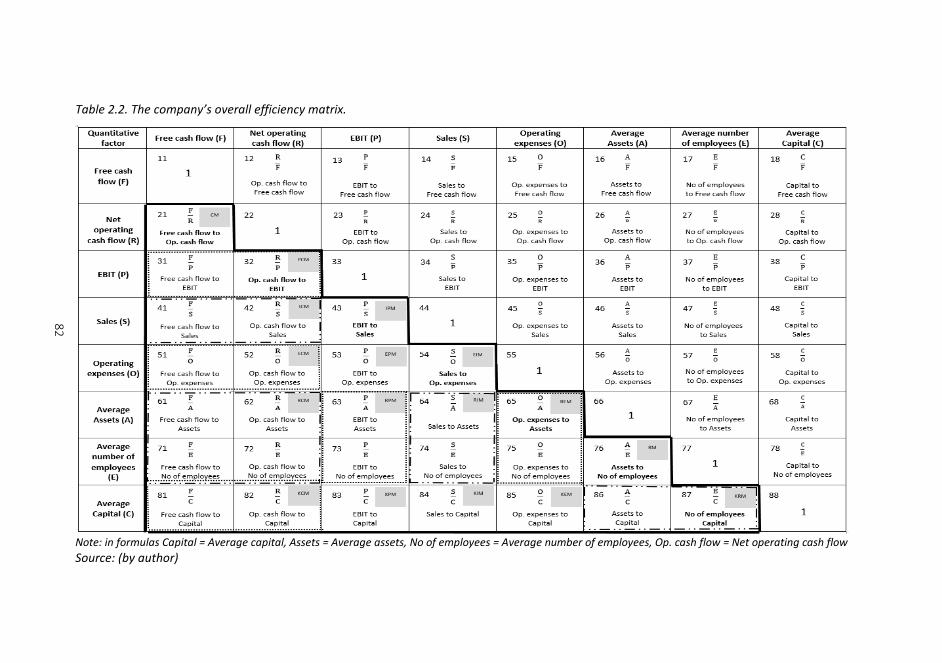
82

Table 2.2. The company’s overall efficiency matrix.

Note: in formulas Capital = Average capital, Assets = Average assets, No of employees = Average number of employees, Op. cash flow = Net operating cash flow Source: (by author)

83

The first quantitative indicator of the company’s overall efficiency matrix is average capital consisting of owners’ equity and loan capital. Since companies have different proportions of owners’ equity and loan capital, the total of these indicators, or the use of total capital, eliminates any difference in the capital structure of companies.

Two resource indicators have been selected for the model: average number of employees and average assets.

In the case of the number of employees and balance sheet information (capital and assets), the arithmetic means of the indicators at the beginning of the year and at the end of the year need to be generated6. This way, these indicators reflecting the current state may be made more comparable to the indicators in an income statement or a cash flow statement, which are period indicators.

In terms of expense indicators, operating expenses, which consist of all the expenses related to earning the sales of a company, have been selected for inclusion in the matrix.

Sales revenue has been selected as the income indicator, since it reflects the income earned from the operating activities of the company and leaves aside the other one-off income.

In the opinion of the author of the thesis, in terms of profit indicators it is most appropriate to use earnings before income tax and interest expenses. As explained previously, this indicator can be compared best in the case of companies with different capital structures. The advantage of earnings before income tax and interest expenses compared to operating profit is that total assets may also include items of assets earning financial income, yet this is not considered by the operating profit indicator. Net profit, however, is affected by differences between countries in the taxation of the profit earned by companies.

In the overall efficiency matrix, there are two cash-based indicators: net operating cash flow and free cash flow. Free cash flow is calculated as a total of net operating cash flow and net investing cash flow. Since both the international standard IAS 7 and the Estonian financial reporting standard permit alternative options for stating cash flows from operating, investment and financing activities, the comparability of cash flow indicators has to be ensured before they are included in an efficiency matrix. When preparing a cash flow statement, a company can choose whether to show paid interest and corporate income tax as the cash flow of financing or operating activities and whether to show interest and dividend received as the investing or operating cash flow. Since neither interest expenses nor income tax expense are included in operating profit, it is more appropriate to state interest paid and corporate income tax as cash flow from financing activities when financial statements are analysed. Interest and dividend received, however, are linked to the use of financial assets; thus, it makes more sense to classify these inflows as investing activities cash flow.

In summary: raising capital enables the entrepreneur to hire labour and invest in assets which, when used, result in operating expenses and thereby create the preconditions for earning income, profit and cash.

In the preparation of financial statements, a practice has become established, whereby more recent financial indicators are presented to the left of less recent

6 In fact, in the case of a moment series, a chronological mean has to be calculated; however, on the condition that only those two sets of data can be used, the period average may be calculated as the arithmetic mean exceptionally. Based on financial information disclosed quarterly, first the average number of employees and the values of capital and assets per quarter can be calculated and then the relevant annual mean indicators may be obtained.

84

indicators. As a result, the author of this doctoral thesis also developed the company’s overall efficiency matrix analogously to previous ones, including quantitative indicators in the matrix in the order of their finality from the right and proceeding onwards to the left.

The company’s overall efficiency matrix is an aggregate model linking intelligibly subindicators related to efficiency. Since it is a structured efficiency matrix, the efficiency field consolidates all the elements that should grow as efficiency rises and reverse efficiency field elements that should decrease as efficiency rises. Hereinafter, this thesis focuses mainly on efficiency field elements. The efficiency field of the company’s overall efficiency matrix presents 17 submatrices out of the 21 submatrices possible. An overview of the qualitative indicators (or, financial ratios) in 17 submatrices is set out in Table 2.3.

If the ratios in the efficiency field are compared to the most common ratios presented in Table 1.4, an overlap may be noticed in the ratios reflecting return on investment, sales profitability and the efficiency of the use of assets. An overall efficiency matrix is not used to analyse the ratios of the structure of assets, since this depends on the field of activity of a company. The biggest difference is in the evaluation of the solvency of a company: in an overall efficiency matrix, several ratios based on cash-based financial indicators are used for this (for example, ratios of capital-cash flow, income-cash flow and profit-cash flow matrices); however, in previous research, accrual-based financial ratios based on relationships among assets and liabilities and owners’ equity have been popular. The advantage of cash-based solvency ratios is their direct relationship to the flow of cash; however, care has to be taken when interpreting the values of ratios. Since the balance sheet, as we know it today, has been in use for about a century longer, the advantage of accrual-based solvency ratios is their more widespread recognition. Unlike the most popular ratios, an overall efficiency matrix devotes more attention to the ratios of the evaluation of the use of labour, cost-efficiency and profit quality.

In an overall efficiency matrix, four submatrices (capital matrix, expense matrix, income matrix, profit matrix) are not represented, since only one indicator is involved in the matrix from the relevant groups of quantitative indicators. This is due to the fact that an overall efficiency matrix uses financial indicators that make companies as comparable to one another as possible. Thus, the aspect that companies have different capital structures has been left aside, since it has an impact on the values of interest expenses and earnings before taxes and net profit. Furthermore, in the estimation of the author of the doctoral thesis, an efficiency matrix with 12 quantitative indicators would be too detailed to be adopted for universal use.

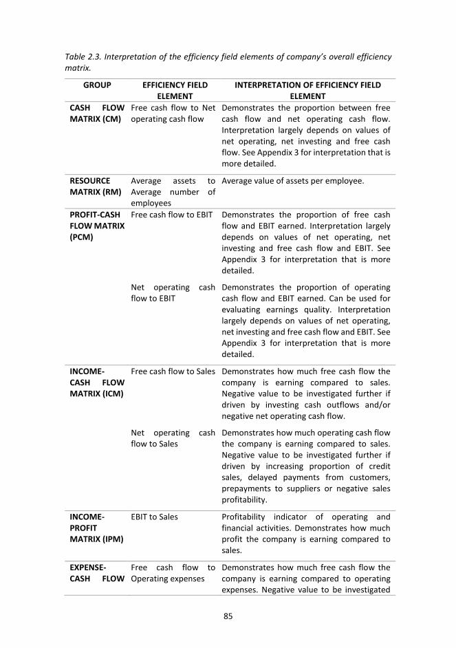
85

Table 2.3. Interpretation of the efficiency field elements of company’s overall efficiency matrix.

GROUP EFFICIENCY FIELD ELEMENT

INTERPRETATION OF EFFICIENCY FIELD ELEMENT

CASH FLOW MATRIX (CM)

Free cash flow to Net operating cash flow

Demonstrates the proportion between free cash flow and net operating cash flow. Interpretation largely depends on values of net operating, net investing and free cash flow. See Appendix 3 for interpretation that is more detailed.

RESOURCE MATRIX (RM)

Average assets to Average number of employees

Average value of assets per employee.

PROFIT-CASH FLOW MATRIX (PCM)

Free cash flow to EBIT

Net operating cash flow to EBIT

Demonstrates the proportion of free cash flow and EBIT earned. Interpretation largely depends on values of net operating, net investing and free cash flow and EBIT. See Appendix 3 for interpretation that is more detailed.

Demonstrates the proportion of operating cash flow and EBIT earned. Can be used for evaluating earnings quality. Interpretation largely depends on values of net operating, net investing and free cash flow and EBIT. See Appendix 3 for interpretation that is more detailed.

INCOME- CASH FLOW MATRIX (ICM)

Free cash flow to Sales

Net operating cash flow to Sales

Demonstrates how much free cash flow the company is earning compared to sales. Negative value to be investigated further if driven by investing cash outflows and/or negative net operating cash flow.

Demonstrates how much operating cash flow the company is earning compared to sales. Negative value to be investigated further if driven by increasing proportion of credit sales, delayed payments from customers, prepayments to suppliers or negative sales profitability.

INCOME-PROFIT MATRIX (IPM)

EBIT to Sales Profitability indicator of operating and financial activities. Demonstrates how much profit the company is earning compared to sales.

EXPENSE-CASH FLOW

Free cash flow to Operating expenses

Demonstrates how much free cash flow the company is earning compared to operating expenses. Negative value to be investigated

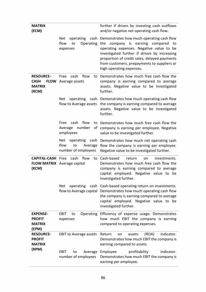
86

MATRIX (ECM)

Net operating cash flow to Operating expenses

further if driven by investing cash outflows and/or negative net operating cash flow.

Demonstrates how much operating cash flow the company is earning compared to operating expenses. Negative value to be investigated further if driven by increasing proportion of credit sales, delayed payments from customers, prepayments to suppliers or high operating expenses.

RESOURCE-CASH FLOW MATRIX (RCM)

Free cash flow to Average assets

Net operating cash flow to Average assets

Free cash flow to Average number of employees

Net operating cash flow to Average number of employees

Demonstrates how much free cash flow the company is earning compared to average assets. Negative value to be investigated further.

Demonstrates how much operating cash flow the company is earning compared to average assets. Negative value to be investigated further.

Demonstrates how much free cash flow the company is earning per employee. Negative value to be investigated further.

Demonstrates how much net operating cash flow the company is earning per employee. Negative value to be investigated further.

CAPITAL-CASH FLOW MATRIX (KCM)

Free cash flow to Average capital

Net operating cash flow to Average capital

Cash-based return on investments. Demonstrates how much free cash flow the company is earning compared to average capital employed. Negative value to be investigated further.

Cash-based operating return on investments. Demonstrates how much operating cash flow the company is earning compared to average capital employed. Negative value to be investigated further.

EXPENSE-PROFIT MATRIX (EPM)

EBIT to Operating expenses

Efficiency of expense usage. Demonstrates how much EBIT the company is earning compared to operating expenses.

RESOURCE-PROFIT MATRIX (RPM)

EBIT to Average assets

EBIT to Average number of employees

Return on assets (ROA) indicator. Demonstrates how much EBIT the company is earning compared to assets.

Employee profitability indicator. Demonstrates how much EBIT the company is earning per employee.

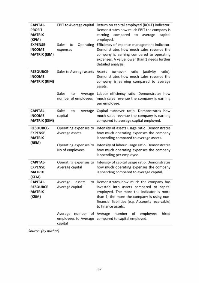
87

CAPITAL-PROFIT MATRIX (KPM)

EBIT to Average capital Return on capital employed (ROCE) indicator. Demonstrates how much EBIT the company is earning compared to average capital employed.

EXPENSE-INCOME MATRIX (EIM)

Sales to Operating expenses

Efficiency of expense management indicator. Demonstrates how much sales revenue the company is earning compared to operating expenses. A value lower than 1 needs further detailed analysis.

RESOURCE-INCOME MATRIX (RIM)

Sales to Average assets

Sales to Average number of employees

Assets turnover ratio (activity ratio). Demonstrates how much sales revenue the company is earning compared to average assets.

Labour efficiency ratio. Demonstrates how much sales revenue the company is earning per employee.

CAPITAL-INCOME MATRIX (KIM)

Sales to Average capital

Capital turnover ratio. Demonstrates how much sales revenue the company is earning compared to average capital employed.

RESOURCE-EXPENSE MATRIX (REM)

Operating expenses to Average assets

Operating expenses to No of employees

Intensity of assets usage ratio. Demonstrates how much operating expenses the company is spending compared to average assets.

Intensity of labour usage ratio. Demonstrates how much operating expenses the company is spending per employee.

CAPITAL-EXPENSE MATRIX (KEM)

Operating expenses to Average capital

Intensity of capital usage ratio. Demonstrates how much operating expenses the company is spending compared to average capital.

CAPITAL-RESOURCE MATRIX (KRM)

Average assets to Average capital

Average number of employees to Average capital

Demonstrates how much the company has invested into assets compared to capital employed. The more the indicator is more than 1, the more the company is using non-financial liabilities (e.g. Accounts receivable) to finance assets.

Average number of employees hired compared to capital employed.

Source: (by author).

88

It can be concluded that compared to the traditional financial analysis and presentation of financial information, the following can be regarded as advantages of the matrix approach (based on (Vensel, 2001, pp. 69–70), (Root, 1987, pp. 6–7) and the opinion of the author of this doctoral thesis):

− The efficiency matrix helps present financial information in a more compact and clearly arranged manner for analysing the efficiency of economic activities and for choosing quantitative initial parameters according to the research objectives. The matrix model, in comparison with other indicator systems, also gives a more comprehensive and systematic picture of the reality to specialists without professional business education.

− The matrix approach is a flexible instrument of analysis, which, by adding or removing initial parameters, allows a more in-depth focus on the weaknesses of a company’s business activities and possibility of improving them.

− The matrix approach helps to analyse all financial ratios in clearly expressed relations and influences.

− During matrix modelling it is possible simultaneously to use different methods of financial analysis (for example, ratio analysis, index analysis, vertical analysis, etc.).

− The matrix approach based analysis of financial information is easy to develop further:

− It is possible to create various multiplicative and additive multifactor systems.

− It is possible to identify absolute changes in quantitative output indicators caused by different components.

− The efficiency matrix helps to divide a set of enterprises into similar parts with the help of cluster analysis.

− Matrix modelling tries to make use of the information arising during financial accounting and the introduction of supplementary reports is usually not presumed.

− Matrix modelling can be easily automated. This subchapter focused on the creation of company’s overall efficiency matrix. As a

result, compared to previous research, the author of current doctoral thesis: − compiled a company’s overall efficiency matrix model, which includes 17

submatrices, − has split input indicators into three groups: capital, resources and expenses, − has split output indicators into three groups: income, profit and cash flow, − proposed the usage of quantitative indicators following the flow of business:

raising capital makes it possible to invest in resources that, through expenses, are transformed into income, profit and cash flow,

− established clear rules on how to rank quantitative indicators within groups of input and output indicators,

− created a summary list of quantitative indicators based on IFRS Taxonomy, − placed a greater emphasis on cash-based financial ratios, since cash is

invested in a company, and loan repayment and dividend payments are also made in cash,

− preapared interpretations of all 28 efficiency field elements of company’s overall efficiency matrix.

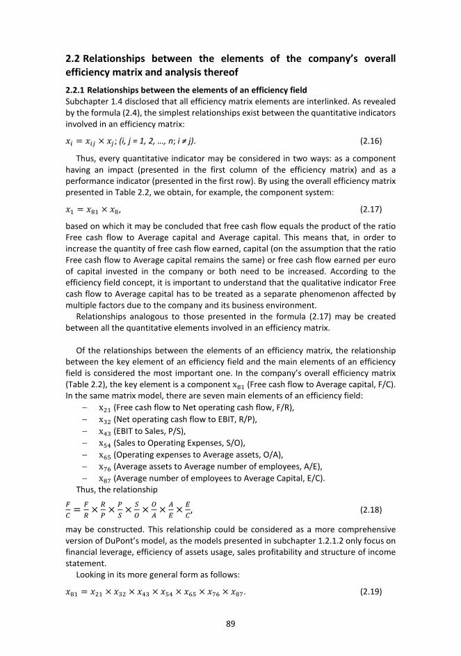
89

2.2 Relationships between the elements of the company’s overall efficiency matrix and analysis thereof 2.2.1 Relationships between the elements of an efficiency field Subchapter 1.4 disclosed that all efficiency matrix elements are interlinked. As revealed by the formula (2.4), the simplest relationships exist between the quantitative indicators involved in an efficiency matrix:

𝑥𝑥𝑝𝑝 = 𝑥𝑥𝑝𝑝𝑖𝑖 × 𝑥𝑥𝑖𝑖 ; (i, j = 1, 2, …, n; i ≠ j). (2.16)

Thus, every quantitative indicator may be considered in two ways: as a component having an impact (presented in the first column of the efficiency matrix) and as a performance indicator (presented in the first row). By using the overall efficiency matrix presented in Table 2.2, we obtain, for example, the component system:

𝑥𝑥1 = 𝑥𝑥81 × 𝑥𝑥8, (2.17)

based on which it may be concluded that free cash flow equals the product of the ratio Free cash flow to Average capital and Average capital. This means that, in order to increase the quantity of free cash flow earned, capital (on the assumption that the ratio Free cash flow to Average capital remains the same) or free cash flow earned per euro of capital invested in the company or both need to be increased. According to the efficiency field concept, it is important to understand that the qualitative indicator Free cash flow to Average capital has to be treated as a separate phenomenon affected by multiple factors due to the company and its business environment.

Relationships analogous to those presented in the formula (2.17) may be created between all the quantitative elements involved in an efficiency matrix.

Of the relationships between the elements of an efficiency matrix, the relationship between the key element of an efficiency field and the main elements of an efficiency field is considered the most important one. In the company’s overall efficiency matrix (Table 2.2), the key element is a component x81 (Free cash flow to Average capital, F/C). In the same matrix model, there are seven main elements of an efficiency field:

− x21 (Free cash flow to Net operating cash flow, F/R), − x32 (Net operating cash flow to EBIT, R/P), − x43 (EBIT to Sales, P/S), − x54 (Sales to Operating Expenses, S/O), − x65 (Operating expenses to Average assets, O/A), − x76 (Average assets to Average number of employees, A/E), − x87 (Average number of employees to Average Capital, E/C).

Thus, the relationship 𝐹𝐹𝐶𝐶

= 𝐹𝐹𝑅𝑅

× 𝑅𝑅𝑃𝑃

× 𝑃𝑃𝑆𝑆

× 𝑆𝑆𝑂𝑂

× 𝑂𝑂𝐴𝐴

× 𝐴𝐴𝐸𝐸

× 𝐸𝐸𝐶𝐶

, (2.18)

may be constructed. This relationship could be considered as a more comprehensive version of DuPont’s model, as the models presented in subchapter 1.2.1.2 only focus on financial leverage, efficiency of assets usage, sales profitability and structure of income statement.

Looking in its more general form as follows:

𝑥𝑥81 = 𝑥𝑥21 × 𝑥𝑥32 × 𝑥𝑥43 × 𝑥𝑥54 × 𝑥𝑥65 × 𝑥𝑥76 × 𝑥𝑥87. (2.19)

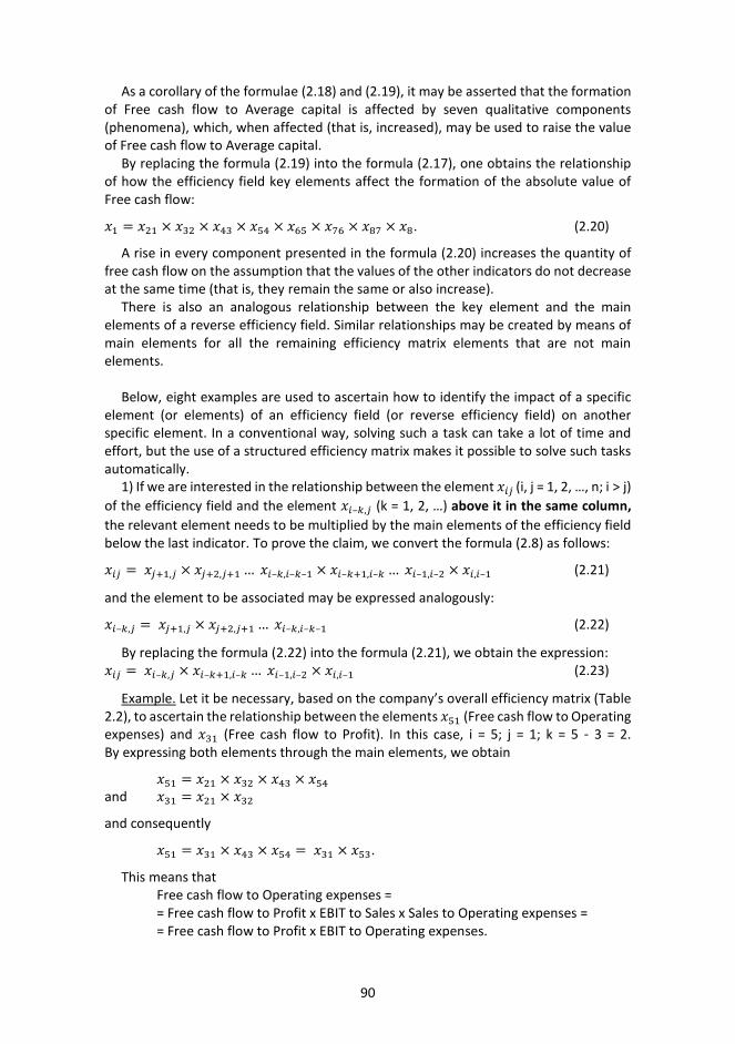
90

As a corollary of the formulae (2.18) and (2.19), it may be asserted that the formation of Free cash flow to Average capital is affected by seven qualitative components (phenomena), which, when affected (that is, increased), may be used to raise the value of Free cash flow to Average capital.

By replacing the formula (2.19) into the formula (2.17), one obtains the relationship of how the efficiency field key elements affect the formation of the absolute value of Free cash flow:

𝑥𝑥1 = 𝑥𝑥21 × 𝑥𝑥32 × 𝑥𝑥43 × 𝑥𝑥54 × 𝑥𝑥65 × 𝑥𝑥76 × 𝑥𝑥87 × 𝑥𝑥8. (2.20)

A rise in every component presented in the formula (2.20) increases the quantity of free cash flow on the assumption that the values of the other indicators do not decrease at the same time (that is, they remain the same or also increase).

There is also an analogous relationship between the key element and the main elements of a reverse efficiency field. Similar relationships may be created by means of main elements for all the remaining efficiency matrix elements that are not main elements.

Below, eight examples are used to ascertain how to identify the impact of a specific element (or elements) of an efficiency field (or reverse efficiency field) on another specific element. In a conventional way, solving such a task can take a lot of time and effort, but the use of a structured efficiency matrix makes it possible to solve such tasks automatically.

1) If we are interested in the relationship between the element 𝑥𝑥𝑝𝑝𝑖𝑖 (i, j = 1, 2, …, n; i > j)of the efficiency field and the element 𝑥𝑥𝑝𝑝–𝑘𝑘,𝑖𝑖 (k = 1, 2, …) above it in the same column, the relevant element needs to be multiplied by the main elements of the efficiency field below the last indicator. To prove the claim, we convert the formula (2.8) as follows:

𝑥𝑥𝑝𝑝𝑖𝑖 = 𝑥𝑥𝑖𝑖+1,𝑖𝑖 × 𝑥𝑥𝑖𝑖+2,𝑖𝑖+1 … 𝑥𝑥𝑝𝑝–𝑘𝑘,𝑝𝑝–𝑘𝑘–1 × 𝑥𝑥𝑝𝑝–𝑘𝑘+1,𝑝𝑝–𝑘𝑘 … 𝑥𝑥𝑝𝑝–1,𝑝𝑝–2 × 𝑥𝑥𝑝𝑝,𝑝𝑝–1 (2.21)

and the element to be associated may be expressed analogously:

𝑥𝑥𝑝𝑝–𝑘𝑘,𝑖𝑖 = 𝑥𝑥𝑖𝑖+1,𝑖𝑖 × 𝑥𝑥𝑖𝑖+2,𝑖𝑖+1 … 𝑥𝑥𝑝𝑝–𝑘𝑘,𝑝𝑝–𝑘𝑘–1 (2.22)

By replacing the formula (2.22) into the formula (2.21), we obtain the expression: 𝑥𝑥𝑝𝑝𝑖𝑖 = 𝑥𝑥𝑝𝑝–𝑘𝑘,𝑖𝑖 × 𝑥𝑥𝑝𝑝–𝑘𝑘+1,𝑝𝑝–𝑘𝑘 … 𝑥𝑥𝑝𝑝–1,𝑝𝑝–2 × 𝑥𝑥𝑝𝑝,𝑝𝑝–1 (2.23)

Example. Let it be necessary, based on the company’s overall efficiency matrix (Table 2.2), to ascertain the relationship between the elements 𝑥𝑥51 (Free cash flow to Operating expenses) and 𝑥𝑥31 (Free cash flow to Profit). In this case, i = 5; j = 1; k = 5 - 3 = 2. By expressing both elements through the main elements, we obtain

𝑥𝑥51 = 𝑥𝑥21 × 𝑥𝑥32 × 𝑥𝑥43 × 𝑥𝑥54 and 𝑥𝑥31 = 𝑥𝑥21 × 𝑥𝑥32

and consequently

𝑥𝑥51 = 𝑥𝑥31 × 𝑥𝑥43 × 𝑥𝑥54 = 𝑥𝑥31 × 𝑥𝑥53.

This means that Free cash flow to Operating expenses = = Free cash flow to Profit х EBIT to Sales х Sales to Operating expenses = = Free cash flow to Profit х EBIT to Operating expenses.

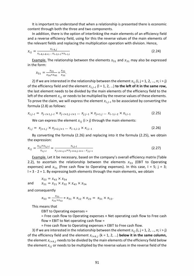
91

It is important to understand that when a relationship is presented there is economic content through both the three and two components.

In addition, there is the option of interlinking the main elements of an efficiency field and a reverse efficiency field, using for this the reverse values of the main elements of the relevant fields and replacing the multiplication operation with division. Hence,

𝑥𝑥𝑝𝑝𝑖𝑖 =𝑥𝑥𝑖𝑖–𝑘𝑘,𝑖𝑖

𝑥𝑥𝑖𝑖–𝑘𝑘,𝑖𝑖–𝑘𝑘+1… 𝑥𝑥𝑖𝑖–2,𝑖𝑖–1×𝑥𝑥𝑖𝑖–1,𝑖𝑖(2.24)

Example. The relationship between the elements 𝑥𝑥51 and 𝑥𝑥31 may also be expressed in the form:

𝑥𝑥51 = 𝑥𝑥31𝑥𝑥34×𝑥𝑥45

= 𝑥𝑥31𝑥𝑥35

.

2) If we are interested in the relationship between the element 𝑥𝑥𝑝𝑝𝑖𝑖 (i, j = 1, 2, …, n; i > j)of the efficiency field and the element 𝑥𝑥𝑝𝑝,𝑖𝑖–𝑇𝑇 (l = 1, 2, …) to the left of it in the same row, the last element needs to be divided by the main elements of the efficiency field to the left of the element 𝑥𝑥𝑝𝑝𝑖𝑖 or needs to be multiplied by the reverse values of these elements. To prove the claim, we will express the element 𝑥𝑥𝑝𝑝,𝑖𝑖–𝑇𝑇 to be associated by converting the formula (2.8) as follows:

𝑥𝑥𝑝𝑝,𝑖𝑖–𝑇𝑇 = 𝑥𝑥𝑖𝑖–𝑇𝑇+1,𝑖𝑖–𝑇𝑇 × 𝑥𝑥𝑖𝑖–𝑇𝑇+2,𝑖𝑖–𝑇𝑇+1 … 𝑥𝑥𝑖𝑖,𝑖𝑖–1 × 𝑥𝑥𝑖𝑖+1,𝑖𝑖 … 𝑥𝑥𝑝𝑝–1,𝑝𝑝–2 × 𝑥𝑥𝑝𝑝,𝑝𝑝–1 (2.25)

We can express the element 𝑥𝑥𝑝𝑝𝑖𝑖 (i > j) through the main elements:

𝑥𝑥𝑝𝑝,𝑖𝑖 = 𝑥𝑥𝑖𝑖+1,𝑖𝑖 × 𝑥𝑥𝑖𝑖+2,𝑖𝑖+1 … 𝑥𝑥𝑝𝑝–1,𝑝𝑝–2 × 𝑥𝑥𝑝𝑝,𝑝𝑝–1 (2.26)

By converting the formula (2.26) and replacing into it the formula (2.25), we obtain the expression:

𝑥𝑥𝑝𝑝𝑖𝑖 =𝑥𝑥𝑖𝑖,𝑖𝑖×𝑥𝑥𝑖𝑖,𝑖𝑖–𝑙𝑙

𝑥𝑥𝑖𝑖,𝑖𝑖–𝑙𝑙=

𝑥𝑥𝑖𝑖,𝑖𝑖–𝑙𝑙

𝑥𝑥𝑖𝑖–𝑙𝑙+1,𝑖𝑖–𝑙𝑙×𝑥𝑥𝑖𝑖–𝑙𝑙+2,𝑖𝑖–𝑙𝑙+1… 𝑥𝑥𝑖𝑖,𝑖𝑖–1(2.27)

Example. Let it be necessary, based on the company’s overall efficiency matrix (Table 2.2), to ascertain the relationship between the elements 𝑥𝑥53 (EBIT to Operating expenses) and 𝑥𝑥51 (Free cash flow to Operating expenses). In this case, I = 5; j = 3; l = 3 - 2 = 1. By expressing both elements through the main elements, we obtain

𝑥𝑥53 = 𝑥𝑥43 × 𝑥𝑥54 and 𝑥𝑥51 = 𝑥𝑥21 × 𝑥𝑥32 × 𝑥𝑥43 × 𝑥𝑥54

and consequently

𝑥𝑥53 = 𝑥𝑥51𝑥𝑥21×𝑥𝑥32

= 𝑥𝑥51 × 𝑥𝑥12 × 𝑥𝑥23 = 𝑥𝑥51 × 𝑥𝑥13.

This means that EBIT to Operating expenses = = Free cash flow to Operating expenses × Net operating cash flow to Free cash flow × EBIT to Net operating cash flow = = Free cash flow to Operating expenses × EBIT to Free cash flow.

3) If we are interested in the relationship between the element 𝑥𝑥𝑝𝑝𝑖𝑖 (i, j = 1, 2, …, n; i > j)of the efficiency field and the element 𝑥𝑥𝑝𝑝+𝑘𝑘,𝑖𝑖 (k = 1, 2, …) below it in the same column, the element 𝑥𝑥𝑝𝑝+𝑘𝑘,𝑖𝑖 needs to be divided by the main elements of the efficiency field below the element 𝑥𝑥𝑝𝑝𝑖𝑖 or needs to be multiplied by the reverse values in the reverse field of the

92

relevant elements. We express the element 𝑥𝑥𝑝𝑝+𝑘𝑘,𝑖𝑖 to be associated through the main elements

𝑥𝑥𝑝𝑝+𝑘𝑘,𝑖𝑖 = 𝑥𝑥𝑖𝑖+1,𝑖𝑖 × 𝑥𝑥𝑖𝑖+2,𝑖𝑖+1 … 𝑥𝑥𝑝𝑝,𝑝𝑝–1 × 𝑥𝑥𝑝𝑝+1,𝑝𝑝 … 𝑥𝑥𝑝𝑝+𝑘𝑘–1,𝑝𝑝+𝑘𝑘–2 × 𝑥𝑥𝑝𝑝+𝑘𝑘,𝑝𝑝+𝑘𝑘–1 (2.28)

and use the formula (2.8), in which the element 𝑥𝑥𝑝𝑝𝑖𝑖 is expressed through the main elements, and obtain the new expression:

𝑥𝑥𝑝𝑝𝑖𝑖 =𝑥𝑥𝑖𝑖+𝑘𝑘,𝑖𝑖×𝑥𝑥𝑖𝑖𝑖𝑖𝑥𝑥𝑖𝑖+𝑘𝑘,𝑖𝑖

=𝑥𝑥𝑖𝑖+𝑘𝑘,𝑖𝑖

𝑥𝑥𝑖𝑖+1,𝑖𝑖… 𝑥𝑥𝑖𝑖+𝑘𝑘–1,𝑖𝑖+𝑘𝑘–2×𝑥𝑥𝑖𝑖+𝑘𝑘,𝑖𝑖+𝑘𝑘–1= 𝑥𝑥𝑝𝑝+𝑘𝑘,𝑖𝑖 × 𝑥𝑥𝑝𝑝,𝑝𝑝+1 … 𝑥𝑥𝑝𝑝+𝑘𝑘–2,𝑝𝑝+𝑘𝑘–1 × 𝑥𝑥𝑝𝑝+𝑘𝑘–1,𝑝𝑝–𝑘𝑘

(2.29)

Example. Let it be necessary, based on the company’s overall efficiency matrix (Table 2.2), to ascertain the relationship between the elements 𝑥𝑥31 (Free cash flow to Profit) and 𝑥𝑥51 (Free cash flow to Operating expenses). In this case, i = 3; j = 1; k = 5 - 3 = 2. By expressing both elements through the main elements, we obtain

𝑥𝑥31 = 𝑥𝑥21 × 𝑥𝑥32 and 𝑥𝑥51 = 𝑥𝑥21 × 𝑥𝑥32 × 𝑥𝑥43 × 𝑥𝑥54

and consequently

𝑥𝑥31 = 𝑥𝑥51𝑥𝑥43×𝑥𝑥54

= 𝑥𝑥51 × 𝑥𝑥34 × 𝑥𝑥45 = 𝑥𝑥51 × 𝑥𝑥35.

This means that Free cash flow to Profit = = Free cash flow to Operating expenses × Sales to Profit × Operating expenses to Sales = = Free cash flow to Operating expenses × Operating expenses to Sales.

4) If we are interested in the relationship between the element 𝑥𝑥𝑝𝑝𝑖𝑖 (i, j = 1, 2, …, n; i > j)of the efficiency field and the element 𝑥𝑥𝑝𝑝,𝑖𝑖+𝑇𝑇 (l = 1, 2, …) to the right of it in the same row, the relevant element 𝑥𝑥𝑝𝑝,𝑖𝑖+𝑇𝑇 needs to be multiplied by the main elements of the efficiency field to the left of the indicator𝑥𝑥𝑝𝑝,𝑖𝑖+𝑇𝑇. To prove the claim, we convert the formula (2.8) as follows:

𝑥𝑥𝑝𝑝𝑖𝑖 = 𝑥𝑥𝑖𝑖+1,𝑖𝑖 × 𝑥𝑥𝑖𝑖+2,𝑖𝑖+1 … 𝑥𝑥𝑖𝑖+𝑇𝑇,𝑖𝑖+𝑇𝑇–1 × 𝑥𝑥𝑖𝑖+𝑇𝑇+1,𝑖𝑖+𝑇𝑇 … 𝑥𝑥𝑝𝑝–1,𝑝𝑝–2 × 𝑥𝑥𝑝𝑝,𝑝𝑝–1 (2.30)

and the element to be associated may be expressed analogously:

𝑥𝑥𝑝𝑝,𝑖𝑖+𝑇𝑇 = 𝑥𝑥𝑖𝑖+𝑇𝑇+1,𝑖𝑖+𝑇𝑇 × 𝑥𝑥𝑖𝑖+𝑇𝑇,𝑖𝑖+𝑇𝑇–1 … 𝑥𝑥𝑝𝑝–1,𝑝𝑝–2 × 𝑥𝑥𝑝𝑝,𝑝𝑝–1 (2.31)

By replacing the formula (2.31) into the formula (2.30), we obtain the expression:

𝑥𝑥𝑝𝑝𝑖𝑖 = 𝑥𝑥𝑖𝑖,𝑖𝑖+𝑙𝑙×𝑥𝑥𝑖𝑖𝑖𝑖𝑥𝑥𝑖𝑖,𝑖𝑖+𝑙𝑙

= 𝑥𝑥𝑝𝑝,𝑖𝑖+𝑇𝑇 × 𝑥𝑥𝑖𝑖+1,𝑖𝑖 × 𝑥𝑥𝑖𝑖+2,𝑖𝑖+1 … 𝑥𝑥𝑖𝑖+𝑇𝑇,𝑖𝑖+𝑇𝑇–1 (2.32)

Example. Let it be necessary, based on the company’s overall efficiency matrix (Table 2.2), to ascertain the relationship between the elements 𝑥𝑥51 (Free cash flow to Operating expenses) and 𝑥𝑥53 (EBIT to Operating expenses). In this case, i = 5; j = 1; l = 3 - 1 = 2. By expressing both elements through the main elements, we obtain

𝑥𝑥51 = 𝑥𝑥21 × 𝑥𝑥32 × 𝑥𝑥43 × 𝑥𝑥54 and 𝑥𝑥53 = 𝑥𝑥43 × 𝑥𝑥54

and consequently

𝑥𝑥51 = 𝑥𝑥53 × 𝑥𝑥21 × 𝑥𝑥32 = 𝑥𝑥53 × 𝑥𝑥31.

93

This means that Free cash flow to Operating expenses = = EBIT to Operating expenses × Free cash flow to Net operating cash flow × Net operating cash flow to Profit = = EBIT to Operating expenses × Free cash flow to Profit.

5) If we are interested in the relationship between the element 𝑥𝑥𝑝𝑝𝑖𝑖 (i, j = 1, 2, …, n; i > j)of the efficiency field and the element 𝑥𝑥𝑝𝑝–𝑘𝑘,𝑖𝑖–𝑇𝑇 (k = 1,2,…; l = 1,2,…) above it to the left, the relevant element 𝑥𝑥𝑝𝑝–𝑘𝑘,𝑖𝑖–𝑇𝑇 needs to be multiplied by the main elements of the efficiency field below it and needs to be divided by the main elements of the efficiency field to the left of the element 𝑥𝑥𝑝𝑝𝑖𝑖 (or multiplied by the relevant main elements of the reverse efficiency field). If i-k > j, to prove the claim, we express the element 𝑥𝑥𝑝𝑝𝑖𝑖 using the formula (2.21):

𝑥𝑥𝑝𝑝𝑖𝑖 = 𝑥𝑥𝑖𝑖+1,𝑖𝑖 × 𝑥𝑥𝑖𝑖+2,𝑖𝑖+1 … 𝑥𝑥𝑝𝑝–𝑘𝑘,𝑝𝑝–𝑘𝑘–1 × 𝑥𝑥𝑝𝑝–𝑘𝑘+1,𝑝𝑝–𝑘𝑘 … 𝑥𝑥𝑝𝑝–1,𝑝𝑝–2 × 𝑥𝑥𝑝𝑝,𝑝𝑝–1

and present the element 𝑥𝑥𝑝𝑝–𝑘𝑘,𝑖𝑖–𝑇𝑇 to be associated in the form:

𝑥𝑥𝑝𝑝–𝑘𝑘,𝑖𝑖–𝑇𝑇 = 𝑥𝑥𝑖𝑖–𝑇𝑇+1,𝑖𝑖–𝑇𝑇 × 𝑥𝑥𝑖𝑖–𝑇𝑇+2,𝑖𝑖–𝑇𝑇+1 … 𝑥𝑥𝑖𝑖,𝑖𝑖–1 × 𝑥𝑥𝑖𝑖+1,𝑖𝑖 … 𝑥𝑥𝑝𝑝–𝑘𝑘,𝑝𝑝–𝑘𝑘–1 (2.33)

By converting the formula (2.21) and replacing into it the formula (2.33), we obtain the expression:

𝑥𝑥𝑝𝑝𝑖𝑖 =𝑥𝑥𝑝𝑝–𝑘𝑘,𝑖𝑖–𝑇𝑇 × 𝑥𝑥𝑝𝑝𝑖𝑖𝑥𝑥𝑝𝑝–𝑘𝑘,𝑖𝑖–𝑇𝑇

=𝑥𝑥𝑝𝑝–𝑘𝑘,𝑖𝑖–𝑇𝑇 × 𝑥𝑥𝑝𝑝–𝑘𝑘+1,𝑝𝑝–𝑘𝑘 … 𝑥𝑥𝑝𝑝–1,𝑝𝑝–2 × 𝑥𝑥𝑝𝑝,𝑝𝑝–1

𝑥𝑥𝑖𝑖–𝑇𝑇+1,𝑖𝑖–𝑇𝑇 × 𝑥𝑥𝑖𝑖–𝑇𝑇+2,𝑖𝑖–𝑇𝑇+1 … 𝑥𝑥𝑖𝑖,𝑖𝑖–1=

= 𝑥𝑥𝑝𝑝–𝑘𝑘,𝑖𝑖–𝑇𝑇 × 𝑥𝑥𝑝𝑝–𝑘𝑘+1,𝑝𝑝–𝑘𝑘 … 𝑥𝑥𝑝𝑝–1,𝑝𝑝–2 × 𝑥𝑥𝑝𝑝,𝑝𝑝–1 × 𝑥𝑥𝑖𝑖–𝑇𝑇,𝑖𝑖–𝑇𝑇+1 × 𝑥𝑥𝑖𝑖–𝑇𝑇+1,𝑖𝑖–𝑇𝑇+2 … 𝑥𝑥𝑖𝑖–1,𝑖𝑖 (2.34)

Example. Let it be necessary, based on the company’s overall efficiency matrix (Table 2.2), to ascertain the relationship between the elements 𝑥𝑥52 (Net operating cash flow to Operating expenses) and 𝑥𝑥31 (Free cash flow to Profit). In this case, i = 5; j = 2; k = 5 - 3 = 2, l = 2 - 1 = 1. By expressing both elements through the main elements, we obtain

𝑥𝑥52 = 𝑥𝑥32 × 𝑥𝑥43 × 𝑥𝑥54 and 𝑥𝑥31 = 𝑥𝑥21 × 𝑥𝑥32

and consequently

𝑥𝑥52 = 𝑥𝑥31×𝑥𝑥52𝑥𝑥31

= 𝑥𝑥31×𝑥𝑥32×𝑥𝑥43×𝑥𝑥54𝑥𝑥21×𝑥𝑥32

= 𝑥𝑥31 × 𝑥𝑥43 × 𝑥𝑥54 × 𝑥𝑥12 = 𝑥𝑥31 × 𝑥𝑥53 × 𝑥𝑥12.

This means that Net operating cash flow to Operating expenses = = Free cash flow to Profit × EBIT to Sales х Sales to Operating expenses × Net operating cash flow to Free cash flow = = Free cash flow to Profit × EBIT to Operating expenses × Net operating cash flow to Free cash flow.

If i-k < j, the element 𝑥𝑥𝑝𝑝–𝑘𝑘,𝑖𝑖–𝑇𝑇 to be associated needs to be multiplied by the main elements of the efficiency field below it, beginning with the element 𝑥𝑥𝑖𝑖+1,𝑖𝑖 in column j and divided by the main elements to the left of the element 𝑥𝑥𝑝𝑝𝑖𝑖 up to the element 𝑥𝑥𝑝𝑝–𝑘𝑘,𝑝𝑝–𝑘𝑘–1 in row i-k or multiplied by the relevant main elements of the reverse efficiency field up to the element 𝑥𝑥𝑝𝑝–𝑘𝑘–1,𝑝𝑝–𝑘𝑘 in row i-k-1. Therefore, we obtain the formula (2.34) expressed as follows:

94

𝑥𝑥𝑝𝑝𝑖𝑖 =𝑥𝑥𝑖𝑖+1,𝑖𝑖 … 𝑥𝑥𝑝𝑝–1,𝑝𝑝–2 × 𝑥𝑥𝑝𝑝,𝑝𝑝–1

𝑥𝑥𝑖𝑖–𝑇𝑇+1,𝑖𝑖–𝑇𝑇 × 𝑥𝑥𝑖𝑖–𝑇𝑇+2,𝑖𝑖–𝑇𝑇+1 … 𝑥𝑥𝑝𝑝–𝑘𝑘,𝑝𝑝–𝑘𝑘–1=

= 𝑥𝑥𝑝𝑝–𝑘𝑘,𝑖𝑖–𝑇𝑇 × 𝑥𝑥𝑖𝑖+1,𝑖𝑖 … 𝑥𝑥𝑝𝑝–1,𝑝𝑝–2 × 𝑥𝑥𝑝𝑝,𝑝𝑝–1 × 𝑥𝑥𝑖𝑖–𝑇𝑇,𝑖𝑖–𝑇𝑇+1 × 𝑥𝑥𝑖𝑖–𝑇𝑇+1,𝑖𝑖–𝑇𝑇+2 … 𝑥𝑥𝑝𝑝–𝑘𝑘–1,𝑝𝑝–𝑘𝑘 (2.35)

6) If we are interested in the relationship between the element 𝑥𝑥𝑝𝑝𝑖𝑖 (i, j = 1, 2, …, n; i > j)of the efficiency field and the element 𝑥𝑥𝑝𝑝–𝑘𝑘,𝑖𝑖+𝑇𝑇 (k = 1, 2, …; l = 1, 2, …) above it to the right, the relevant element 𝑥𝑥𝑝𝑝–𝑘𝑘,𝑖𝑖+𝑇𝑇 needs to be multiplied by the main elements of the efficiency field below it and the main elements of the efficiency field to the left. To prove the claim, we convert for the expression of the element 𝑥𝑥𝑝𝑝𝑖𝑖 the formula (2.21) as follows:

𝑥𝑥𝑝𝑝𝑖𝑖 = 𝑥𝑥𝑖𝑖+1,𝑖𝑖 × 𝑥𝑥𝑖𝑖+2,𝑖𝑖+1 … 𝑥𝑥𝑖𝑖+𝑇𝑇,𝑖𝑖+𝑇𝑇–1 × 𝑥𝑥𝑖𝑖+𝑇𝑇+1,𝑖𝑖+𝑇𝑇 … 𝑥𝑥𝑝𝑝–𝑘𝑘,𝑝𝑝–𝑘𝑘–1 × 𝑥𝑥𝑝𝑝–𝑘𝑘+1,𝑝𝑝–𝑘𝑘 … 𝑥𝑥𝑝𝑝–1,𝑝𝑝–2 ×𝑥𝑥𝑝𝑝,𝑝𝑝–1 (2.36)

and present the element 𝑥𝑥𝑝𝑝–𝑘𝑘,𝑖𝑖+𝑇𝑇 to be associated in the form:

𝑥𝑥𝑝𝑝–𝑘𝑘,𝑖𝑖+𝑇𝑇 = 𝑥𝑥𝑖𝑖+𝑇𝑇+1,𝑖𝑖+𝑇𝑇 × 𝑥𝑥𝑖𝑖+𝑇𝑇+2,𝑖𝑖+𝑇𝑇+1 … 𝑥𝑥𝑝𝑝–𝑘𝑘–1,𝑝𝑝–𝑘𝑘–2 × 𝑥𝑥𝑝𝑝–𝑘𝑘,𝑝𝑝–𝑘𝑘–1 (2.37)

By replacing the formula (2.37) into the formula (2.36), we obtain the expression:

𝑥𝑥𝑝𝑝𝑖𝑖 = 𝑥𝑥𝑖𝑖–𝑘𝑘,𝑖𝑖+𝑙𝑙×𝑥𝑥𝑖𝑖𝑖𝑖𝑥𝑥𝑖𝑖–𝑘𝑘,𝑖𝑖+𝑙𝑙

= 𝑥𝑥𝑝𝑝–𝑘𝑘,𝑖𝑖+𝑇𝑇 × 𝑥𝑥𝑖𝑖+1,𝑖𝑖 × 𝑥𝑥𝑖𝑖+2,𝑖𝑖+1 … 𝑥𝑥𝑖𝑖+𝑇𝑇,𝑖𝑖+𝑇𝑇–1 × 𝑥𝑥𝑝𝑝–𝑘𝑘+1,𝑝𝑝–𝑘𝑘 … 𝑥𝑥𝑝𝑝–1,𝑝𝑝–2 × 𝑥𝑥𝑝𝑝,𝑝𝑝–1(2.38)

Example. Let it be necessary, based on the company’s overall efficiency matrix (Table 2.2) to ascertain the relationship between the elements 𝑥𝑥51 (Free cash flow to Operating expenses) and 𝑥𝑥42 (Net operating cash flow to Sales). In this case, i = 5; j = 1; k = 5 - 4 = 1, l = 2 - 1 = 1. By expressing both elements through the main elements, we obtain

𝑥𝑥51 = 𝑥𝑥21 × 𝑥𝑥32 × 𝑥𝑥43 × 𝑥𝑥54 and 𝑥𝑥42 = 𝑥𝑥32 × 𝑥𝑥43

and consequently

𝑥𝑥51 = 𝑥𝑥42 × 𝑥𝑥21 × 𝑥𝑥54.

This means that Free cash flow to Operating expenses = = Net operating cash flow to Sales × Free cash flow to Net operating cash flow × Sales to Operating expenses.

7) If we are interested in the relationship between the element 𝑥𝑥𝑝𝑝𝑖𝑖 (i, j = 1, 2, …, n; i > j)of the efficiency field and the element 𝑥𝑥𝑝𝑝+𝑘𝑘,𝑖𝑖+𝑇𝑇 (k = 1, 2, … ; l = 1 , 2, …) ,…) below it to the right, the element 𝑥𝑥𝑝𝑝+𝑘𝑘,𝑖𝑖+𝑇𝑇 needs to be multiplied by the main elements of the efficiency field to the left of it and needs to be divided by the main elements of the efficiency field below the element 𝑥𝑥𝑝𝑝𝑖𝑖 (or multiplied by the relevant main elements of the reverse efficiency field). If i > j+l, by using the formula (2.8) element 𝑥𝑥𝑝𝑝𝑖𝑖 may be expressed through the main elements as follows:

𝑥𝑥𝑝𝑝𝑖𝑖 = 𝑥𝑥𝑖𝑖+1,𝑖𝑖 × 𝑥𝑥𝑖𝑖+2,𝑖𝑖+1 … 𝑥𝑥𝑖𝑖+𝑇𝑇,𝑖𝑖+𝑇𝑇–1 × 𝑥𝑥𝑖𝑖+𝑇𝑇+1,𝑖𝑖+𝑇𝑇 … 𝑥𝑥𝑝𝑝–1,𝑝𝑝–2 × 𝑥𝑥𝑝𝑝,𝑝𝑝–1 (2.39)

𝑥𝑥𝑝𝑝+𝑘𝑘,𝑖𝑖+𝑇𝑇 = 𝑥𝑥𝑖𝑖+𝑇𝑇+1,𝑖𝑖+𝑇𝑇 × 𝑥𝑥𝑖𝑖+𝑇𝑇+2,𝑖𝑖+𝑇𝑇+1 … 𝑥𝑥𝑝𝑝,𝑝𝑝–1 × 𝑥𝑥𝑝𝑝+1,𝑝𝑝 … 𝑥𝑥𝑝𝑝+𝑘𝑘–1,𝑝𝑝+𝑘𝑘–2 × 𝑥𝑥𝑝𝑝+𝑘𝑘,𝑝𝑝+𝑘𝑘–1 (2.40)

By converting the formula (2.39) and replacing into it the formula (2.40), we obtain the expression:

95

𝑥𝑥𝑝𝑝𝑖𝑖 =𝑥𝑥𝑝𝑝+𝑘𝑘,𝑖𝑖+𝑇𝑇 × 𝑥𝑥𝑝𝑝𝑖𝑖𝑥𝑥𝑝𝑝+𝑘𝑘,𝑖𝑖+𝑇𝑇

=𝑥𝑥𝑝𝑝+𝑘𝑘,𝑖𝑖+𝑇𝑇 × 𝑥𝑥𝑖𝑖+1,𝑖𝑖 × 𝑥𝑥𝑖𝑖+2,𝑖𝑖+1 … 𝑥𝑥𝑖𝑖+𝑇𝑇,𝑖𝑖+𝑇𝑇–1

𝑥𝑥𝑝𝑝+1,𝑝𝑝 … 𝑥𝑥𝑝𝑝+𝑘𝑘–1,𝑝𝑝+𝑘𝑘–2 × 𝑥𝑥𝑝𝑝+𝑘𝑘,𝑝𝑝+𝑘𝑘–1=

= 𝑥𝑥𝑝𝑝+𝑘𝑘,𝑖𝑖+𝑇𝑇 × 𝑥𝑥𝑖𝑖+1,𝑖𝑖 × 𝑥𝑥𝑖𝑖+2,𝑖𝑖+1 … 𝑥𝑥𝑖𝑖+𝑇𝑇,𝑖𝑖+𝑇𝑇–1 × 𝑥𝑥𝑝𝑝,𝑝𝑝+1 … 𝑥𝑥𝑝𝑝+𝑘𝑘–2,𝑝𝑝+𝑘𝑘–1 × 𝑥𝑥𝑝𝑝+𝑘𝑘–1,𝑝𝑝+𝑘𝑘 (2.41)

Example. Let it be necessary, based on the company’s overall efficiency matrix (Table 2.2), to ascertain the relationship between the elements 𝑥𝑥41 (Free cash flow to Sales) and 𝑥𝑥52 (Net operating cash flow to Operating expenses). In this case, i = 4; j = 1; k = 5 - 4 = 1, l = 2 - 1 = 1. By expressing both elements through the main elements, we obtain

𝑥𝑥41 = 𝑥𝑥21 × 𝑥𝑥32 × 𝑥𝑥43 and 𝑥𝑥52 = 𝑥𝑥32 × 𝑥𝑥43 × 𝑥𝑥54

and consequently

𝑥𝑥41 = 𝑥𝑥52×𝑥𝑥41𝑥𝑥52

= 𝑥𝑥52×𝑥𝑥21𝑥𝑥54

= 𝑥𝑥52 × 𝑥𝑥21 × 𝑥𝑥45.

This means that Free cash flow to Sales = = Net operating cash flow to Operating expenses × Free cash flow to Net operating cash flow × Operating expenses to Sales.

If i < j+l, there are no overlapping main elements. The relationship between the elements 𝑥𝑥𝑝𝑝𝑖𝑖 and 𝑥𝑥𝑝𝑝+𝑘𝑘,𝑖𝑖+𝑇𝑇 has to be formulated as follows: if we are interested in the relationship between the element xij (i, j = 1, 2, …, n; i > j) of the efficiency field and the element 𝑥𝑥𝑝𝑝+𝑘𝑘,𝑖𝑖+𝑇𝑇 (k = 1, 2, …; l= 1, 2, …) below it to the right, the element 𝑥𝑥𝑝𝑝+𝑘𝑘,𝑖𝑖+𝑇𝑇 needs to be multiplied by the main elements of the efficiency field to the left of it up to the main element 𝑥𝑥𝑝𝑝,𝑝𝑝–1 in row i and needs to be divided by the main elements of the efficiency field below the element 𝑥𝑥𝑝𝑝𝑖𝑖 , beginning with the element 𝑥𝑥𝑖𝑖+𝑇𝑇,𝑖𝑖+𝑇𝑇+1 in row j+l+1. Therefore, we obtain the formula (2.41) expressed as follows:

𝑥𝑥𝑝𝑝𝑖𝑖 =𝑥𝑥𝑝𝑝+𝑘𝑘,𝑖𝑖+𝑇𝑇 × 𝑥𝑥𝑖𝑖+1,𝑖𝑖 × 𝑥𝑥𝑖𝑖+2,𝑖𝑖+1 … 𝑥𝑥𝑝𝑝,𝑝𝑝–1𝑥𝑥𝑖𝑖+𝑇𝑇+1,𝑖𝑖+𝑇𝑇 … 𝑥𝑥𝑝𝑝+𝑘𝑘–1,𝑝𝑝+𝑘𝑘–2 × 𝑥𝑥𝑝𝑝+𝑘𝑘,𝑝𝑝+𝑘𝑘–1

=

= 𝑥𝑥𝑝𝑝+𝑘𝑘,𝑖𝑖+𝑇𝑇 × 𝑥𝑥𝑖𝑖+1,𝑖𝑖 × 𝑥𝑥𝑖𝑖+2,𝑖𝑖+1 … 𝑥𝑥𝑝𝑝,𝑝𝑝–1 × 𝑥𝑥𝑖𝑖+𝑇𝑇,𝑖𝑖+𝑇𝑇+1 … 𝑥𝑥𝑝𝑝+𝑘𝑘–2,𝑝𝑝+𝑘𝑘–1 × 𝑥𝑥𝑝𝑝+𝑘𝑘–1,𝑝𝑝+𝑘𝑘 (2.42)

8) If we are interested in the relationship between the element 𝑥𝑥𝑝𝑝𝑖𝑖 (i, j = 1, 2, …, n; i > j)of the efficiency field and the element 𝑥𝑥𝑝𝑝+𝑘𝑘,𝑖𝑖–𝑇𝑇 (k = 1, 2, …; l = 1, 2, …) below it to the left, the element 𝑥𝑥𝑝𝑝+𝑘𝑘,𝑖𝑖–𝑇𝑇 needs to be divided by the main elements of the efficiency field to the left of and below the element 𝑥𝑥𝑝𝑝𝑖𝑖 (or multiplied by the relevant main elements of the reverse efficiency field). By using the formula (2.8), the elements 𝑥𝑥𝑝𝑝𝑖𝑖 and 𝑥𝑥𝑝𝑝+𝑘𝑘,𝑖𝑖–𝑇𝑇 may be expressed through the main elements as follows:

𝑥𝑥𝑝𝑝𝑖𝑖 = 𝑥𝑥𝑖𝑖+1,𝑖𝑖 × 𝑥𝑥𝑖𝑖+2,𝑖𝑖+1 … 𝑥𝑥𝑝𝑝–1,𝑝𝑝–2 × 𝑥𝑥𝑝𝑝,𝑝𝑝–1 (2.43)

𝑥𝑥𝑝𝑝+𝑘𝑘,𝑖𝑖–𝑇𝑇 = 𝑥𝑥𝑖𝑖–𝑇𝑇+1,𝑖𝑖–𝑇𝑇 × 𝑥𝑥𝑖𝑖–𝑇𝑇+2,𝑖𝑖–𝑇𝑇+1 … 𝑥𝑥𝑖𝑖,𝑖𝑖–1 × 𝑥𝑥𝑖𝑖+1,𝑖𝑖 … 𝑥𝑥𝑝𝑝,𝑝𝑝–1 × 𝑥𝑥𝑝𝑝+1,𝑝𝑝 … 𝑥𝑥𝑝𝑝+𝑘𝑘–1,𝑝𝑝+𝑘𝑘–2 ×𝑥𝑥𝑝𝑝+𝑘𝑘,𝑝𝑝+𝑘𝑘–1 (2.44)

By converting the formula (2.43) and replacing into it the formula (2.44), we obtain the expression:

𝑥𝑥𝑝𝑝𝑖𝑖 =𝑥𝑥𝑝𝑝+𝑘𝑘,𝑖𝑖–𝑇𝑇 × 𝑥𝑥𝑝𝑝𝑖𝑖𝑥𝑥𝑝𝑝+𝑘𝑘,𝑖𝑖–𝑇𝑇

=𝑥𝑥𝑝𝑝+𝑘𝑘,𝑖𝑖–𝑇𝑇

𝑥𝑥𝑖𝑖–𝑇𝑇+1,𝑖𝑖–𝑇𝑇 × 𝑥𝑥𝑖𝑖–𝑇𝑇+2,𝑖𝑖–𝑇𝑇+1 … 𝑥𝑥𝑖𝑖,𝑖𝑖–1 × 𝑥𝑥𝑝𝑝+1,𝑝𝑝 … 𝑥𝑥𝑝𝑝+𝑘𝑘–1,𝑝𝑝+𝑘𝑘–2 × 𝑥𝑥𝑝𝑝+𝑘𝑘,𝑝𝑝+𝑘𝑘–1=

= 𝑥𝑥𝑝𝑝+𝑘𝑘,𝑖𝑖–𝑇𝑇 × 𝑥𝑥𝑖𝑖–𝑇𝑇,𝑖𝑖–𝑇𝑇+1 × 𝑥𝑥𝑖𝑖–𝑇𝑇+1,𝑖𝑖–𝑇𝑇+2 … 𝑥𝑥𝑖𝑖–1,𝑖𝑖 × 𝑥𝑥𝑝𝑝,𝑝𝑝+1 … 𝑥𝑥𝑝𝑝+𝑘𝑘–2,𝑝𝑝+𝑘𝑘–1 × 𝑥𝑥𝑝𝑝+𝑘𝑘–1,𝑝𝑝+𝑘𝑘 (2.45)

96

Example. Let it be necessary, based on the company’s overall efficiency matrix (Table 2.2), to ascertain the relationship between the elements 𝑥𝑥42 (Net operating cash flow to Sales) and 𝑥𝑥51 (Free cash flow to Operating expenses). In this case, i = 4; j = 2; k = 5 -4 = 1, l = 2 - 1 = 1. By expressing both elements through the main elements, we obtain

𝑥𝑥42 = 𝑥𝑥32 × 𝑥𝑥43 and 𝑥𝑥51 = 𝑥𝑥21 × 𝑥𝑥32 × 𝑥𝑥43 × 𝑥𝑥54

and consequently

𝑥𝑥42 = 𝑥𝑥51×𝑥𝑥42𝑥𝑥51

= 𝑥𝑥51𝑥𝑥21×𝑥𝑥54

= 𝑥𝑥51 × 𝑥𝑥12 × 𝑥𝑥45.

This means that Net operating cash flow to Sales = = Free cash flow to Operating expenses × Net operating cash flow to Free cash flow × Operating expenses to Sales.

Since a reverse efficiency field is the mirror image of an efficiency field, similar relationships may also be established for the relationships between the elements of the reverse efficiency field. For interested readers, these relationships are set out in Appendix 4.

The above examples confirm that it is always possible to ascertain the impact of every specific element of an efficiency field or reverse efficiency field on another specific element, because of which the solution of practical analysis tasks becomes simpler. When interpreting results of analysis, it is important to consider that every element of an efficiency matrix has to be treated as a separate phenomenon caused by many factors resulting from the company and from the business environment surrounding it.

2.2.2 Calculation and analysis of overall efficiency indicators Subchapter 1.1 revealed that discussion of what the most sensible way to measure efficiency is has been going on for a while now. Often, the calculation of some ratio or other is adopted as the basis and there is discussion of what should be in the numerators and denominators of ratios that best characterise efficiency. Subchapter 1.4 suggested that the use of one or a few ratios never provides an exhaustive answer about the level of the economic efficiency of a company as a multi-faceted qualitative phenomenon or about change therein. The latter can only be reflected adequately by a field of relationships created out of the key financial ratios on the principle of full systemicity, which is represented more appropriately as a matrix. It is important to be aware that, to solve analysis tasks, qualitative indicators in one row or column of a matrix are not sufficient, and consideration has to be given to all the elements of an efficiency field (or reverse efficiency field). Subchapter 1.4 also revealed that an efficiency field based on five quantitative indicators created on the principle of full systemicity, consists of 20 financial ratios to be analysed. As a result of the involvement of ten initial quantitative indicators, the field consists of as many as 45 indicators that help to evaluate efficiency levels and the reasons for change therein.

As revealed by the foregoing, the matrix concept of economic efficiency denies the possibility of reflecting the level of the economic efficiency of a company and of change therein in a single figure. In reality, a further problem often needs to be solved when efficiency is measured: ranking economic entities based on their efficiency. This cannot

97

be done using an efficiency matrix, since one economic entity may prove better based on the value of one matrix element, the second/third economic entity based on the second/third matrix element, etc.

Whereas analysing the efficiency field is mostly relevant to discovering the internal reserves of an economic entity, the ranking problem plays an important role when it comes to the management and work organisation of economic entities. Once it is known which economic entity has a higher level of efficiency and which one a lower level of efficiency, it is known who is to be acknowledged and who is to be encouraged to catch up to the others. This type of information has important implications at all management levels (department, company, field of activity, country and others). To be able to develop ranking lists, one needs to know an indicator expressed as a single number measuring either the level of efficiency (static ranking problem) or change therein (dynamic ranking problem).

Subchapter 1.4 revealed that in previous research the creation of an overall efficiency indicator based on an efficiency matrix has been engaged in by Mereste (1980), Mereste (1981), Root (1981) and Vensel (1984). The author of this thesis holds the view that, since the calculation of an overall efficiency indicator is based on an index matrix calculated on the basis of an efficiency matrix and the indices are multiples, the most accurate overall efficiency indicator may be obtained by applying the geometric mean and by using the indices of all the efficiency field elements. Thus, the author of this doctoral thesis agrees that the computing rule proposed by Root (1981) is best suited for obtaining the overall efficiency indicator. Based on the example presented in subchapter 1.4 (formulae 1.17 and 1.18), the author of this thesis includes as an additional constraint the requirement that an efficiency matrix has to involve an even number of quantitative indicators, since in this case every quantitative indicator is considered in the calculation of the geometric mean.

Root (1981) showed that an overall efficiency indicator may be obtained by means of either the growth indices of all the elements of an efficiency field (formula 1.15) or the growth indices of quantitative indicators (formula 1.16).

2.2.2.1 Solving a static ranking problem based on the company’s overall efficiency matrix Solving a static ranking problem means solving the problem of the complex comparative analysis of the efficiency of an economic entity and, thereby, finding unused reserves. The overall indicator calculated in the course of it is referred to by the author of the thesis as the benchmark index of company’s overall efficiency (BICOE). First, it has to be decided what to adopt as the benchmark. For this, the following are suitable in comparative analysis carried out at the level of the company:

1) data of one’s own company,2) market leader data,3) average indicators of all the companies in the reference group.

In addition, calculation of the benchmark index of company’s overall efficiency may run into the problem of negative values, discussed in subchapter 1.2.3. As a result, the calculation of a benchmark index of company’s overall efficiency is subject to the assumption that the reference group (including the indicators or average indicators of the benchmark company) should include only those companies whose profit (EBIT) and cash flow group indicators are all positive. In the case of companies making a loss, having a negative net cash flow from their business activities and/or having negative value of

98

free cash flow, there is no point in obtaining an efficiency index and, in some instances, it is also technically impossible.

The first option for calculating BICOE is based on the growth indices of all the elements of an efficiency field. In this case, the following steps need to be performed:

1) Develop overall efficiency matrices based on the financial information of allthe companies in a comparable population for the same period.

2) Divide the efficiency field elements of all the companies by the efficiency field elements adopted as the benchmark (formula 2.46). This results in thecompletion of a comparative efficiency matrix (Table 2.4), whose everyelement 𝑐𝑐𝑝𝑝𝑖𝑖 is the quotient of the elements of the efficiency fields for thesame period of a company analysed and of the company selected as thebenchmark.

𝑐𝑐𝑝𝑝𝑖𝑖𝐴𝐴/0 =

𝑥𝑥𝑖𝑖𝑖𝑖𝐴𝐴

𝑥𝑥𝑖𝑖𝑖𝑖0 , (2.46)

where cijA/0 – element of the efficiency field of a comparative matrix,𝑥𝑥𝑝𝑝𝑖𝑖𝐴𝐴 – value of an efficiency field element of the company analysed (A), 𝑥𝑥𝑝𝑝𝑖𝑖0 – value of the efficiency field element of the company (0) selected as the benchmark for the same period.

3) Calculate a benchmark index of company’s overall efficiency (BICOE):

𝐵𝐵𝐼𝐼𝐶𝐶𝑅𝑅𝑅𝑅 = �∏𝑐𝑐𝑝𝑝𝑖𝑖𝐴𝐴/0

𝑛𝑛2–𝑛𝑛2

, (2.47)

where 𝑐𝑐ijA/0 – all efficiency field elements of comparative matrix,

n – number of quantitative indicators in the model. 4) Rank companies based on the numerical value of the benchmark index of

overall efficiency in descending order. As a result, a data series is obtained;in it, companies with relatively higher efficiency levels are in the front andcompanies with lower levels are in the back.

5) By analysing the elements of a comparative matrix, ascertain the mainreasons why the company analysed has placed in this position specifically onthe ranking list of change in efficiency levels. The more the value of thespecific element 𝑐𝑐𝑝𝑝𝑖𝑖 exceeds one, the more efficient the company is in termsof this indicator. And vice versa, the more the value of the specific element𝑐𝑐𝑝𝑝𝑖𝑖 is below one, the lower the efficiency of the company is in terms of thegiven indicator, or the more reserves the company analysed has comparedto the benchmark company.

6) Set objectives and develop proposals as to what activities need to be carriedout in order to raise efficiency at the company analysed. The objective maybe the achievement of the best or mean level in the reference group or theachievement of the level of a company a few positions higher than that ofthe company analysed.

99

Table 2.4. Efficiency matrix of comparative coefficients (based on company’s overall efficiency matrix)

Note: QI= quantitative indicator (see Table 2.2 for the abbreviations). Source: (by author)

The other option to obtain the value of BICOE is without developing a company’s overall efficiency matrix or a multiplier matrix based on it. Considering that there are eight quantitative initial indicators in the overall efficiency matrix of a company, based on the formula (1.16) and using the benchmark index 𝐶𝐶𝑖𝑖 of the quantitative indicator, we obtain:

𝐵𝐵𝐼𝐼𝐶𝐶𝑅𝑅𝑅𝑅 = ��𝐶𝐶𝑖𝑖8–(2𝑖𝑖−1)

8

𝑖𝑖=1

28=

= �𝐶𝐶1728 × �𝐶𝐶25

28 × �𝐶𝐶3328 × �𝐶𝐶41

28 × �𝐶𝐶5−128 × �𝐶𝐶6−3

28 × �𝐶𝐶7−528 × �𝐶𝐶8−7

28 . (2.48)

The numerical values of BICOE need to be compared with 1. For example: 1) if the value of BICOE is 1.25, the overall efficiency level of the company

analysed is 25% higher than in the case of the benchmark company (or reference group mean),

2) if the value of BICOE is 0.8, the overall efficiency level of the companyanalysed is 20% lower than in the case of the benchmark company (or reference group mean).

The numerical values of BICOE calculated using both computing rules are equal. The advantage of the first approach is that based on the elements of the efficiency field of a multiplier matrix one can analyse in detail the formation of both the numerical value of BICOE and of the position of the company on the ranking list. The advantage of the second approach is that the numerical value of BICOE can be calculated with significantly less efforts; however, its drawback is the fact that there is no option for detailed analysis similar to the first approach.

100

2.2.2.2 Solving a dynamic ranking problem based on the company’s overall efficiency matrix

Whereas a static ranking problem makes it possible to identify unused reserves, the solution of a dynamic ranking problem brings clarity on how the overall efficiency levels of companies have changed compared to the reference period. The reference period may be chosen freely and may be a previous month, quarter, year or even a period from five years ago. In this thesis, the overall indicator obtained in the course of solving a dynamic ranking problem is referred to as the growth index of a company’s overall efficiency (GICOE). In order to find out at which companies efficiency levels have changed more and at which companies they have changed less, companies need to be ranked by their value of GICOE.

Similarly to BICOE, GICOE is also subject to the assumption that it may be calculated in the case of companies where all quantitative indicators have positive values.

The first option for calculating GICOE is based on the growth indices of all the elements of an efficiency field. In this case, the following steps need to be performed:

1) Develop overall efficiency matrices based on the financial information of allthe companies in a reference group for the period analysed and for the baseperiod.

2) Divide the efficiency field elements of all the companies for the periodanalysed by the efficiency field elements for the base period (formula 2.49).This results in the completion of an efficiency index matrix (Table 2.5), whoseevery element 𝑖𝑖𝑝𝑝𝑖𝑖 is the quotient of the elements of the efficiency fields of agiven company for the period analysed and the base period.

𝑖𝑖𝑝𝑝𝑖𝑖𝑁𝑁1/𝑁𝑁0 =

𝑥𝑥𝑖𝑖𝑖𝑖𝑡𝑡1

𝑥𝑥𝑖𝑖𝑖𝑖𝑡𝑡0 , (2.49)

where iijt1/t0 – element of the efficiency field of an index matrix (growth

index), xijt1 – value of an efficiency field element of the company analysed

for the period analysed, xijt0 – value of the efficiency field element of the company

analysed for the previous period. 3) Calculate a growth index of company’s overall efficiency (GICOE):

𝐺𝐺𝐼𝐼𝐶𝐶𝑅𝑅𝑅𝑅 = �∏𝑖𝑖𝑝𝑝𝑖𝑖𝑁𝑁𝑘𝑘/𝑁𝑁0

𝑛𝑛2–𝑛𝑛2

, (2.50)

where 𝑖𝑖𝑝𝑝𝑖𝑖𝑁𝑁𝑘𝑘/𝑁𝑁0 – all index matrix efficiency field elements,

n – number of quantitative indicators in the model. 4) Rank companies based on the numerical value of the growth index of overall

efficiency in descending order. As a result, a data series is obtained; in it,companies with relatively better efficiency growth rate levels are in the frontand those with lower levels are in the back.

5) By analysing the elements of an index matrix, ascertain the main reasons why the company analysed has placed in this position specifically on the rankinglist of change in efficiency levels. The more the value of the specific element𝑖𝑖𝑝𝑝𝑖𝑖 exceeds one, the more the indicator considered has contributed to the

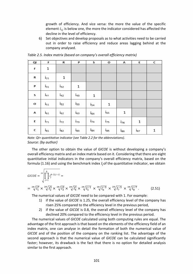
101

growth of efficiency. And vice versa: the more the value of the specific element 𝑖𝑖𝑝𝑝𝑖𝑖 is below one, the more the indicator considered has affected the decline in the level of efficiency.

6) Set objectives and develop proposals as to what activities need to be carriedout in order to raise efficiency and reduce areas lagging behind at the company analysed.

Table 2.5. Index matrix (based on company’s overall efficiency matrix)

Note: QI= quantitative indicator (see Table 2.2 for the abbreviations). Source: (by author)

The other option to obtain the value of GICOE is without developing a company’s overall efficiency matrix and an index matrix based on it. Considering that there are eight quantitative initial indicators in the company’s overall efficiency matrix, based on the formula (1.16) and using the benchmark index 𝐼𝐼𝑖𝑖of the quantitative indicator, we obtain

𝐺𝐺𝐼𝐼𝐶𝐶𝑅𝑅𝑅𝑅 = ��𝐼𝐼𝑖𝑖8–(2𝑖𝑖−1)

8

𝑖𝑖=1

28

=

= �𝐼𝐼1728 × �𝐼𝐼25

28 × �𝐼𝐼3328 × �𝐼𝐼41

28 × �𝐼𝐼5−128 × �𝐼𝐼6−3

28 × �𝐼𝐼7−528 × �𝐼𝐼8−7

28 . (2.51)

The numerical values of GICOE need to be compared with 1. For example: 1) if the value of GICOE is 1.25, the overall efficiency level of the company has

risen 25% compared to the efficiency level in the previous period, 2) if the value of GICOE is 0.8, the overall efficiency level of the company has

declined 20% compared to the efficiency level in the previous period. The numerical values of GICOE calculated using both computing rules are equal. The

advantage of the first approach is that based on the elements of the efficiency field of an index matrix, one can analyse in detail the formation of both the numerical value of GICOE and of the position of the company on the ranking list. The advantage of the second approach is that the numerical value of GICOE can be calculated significantly faster; however, its drawback is the fact that there is no option for detailed analysis similar to the first approach.

102

The calculation formula for GICOE presupposes that elements of the efficiency field of an index matrix have been calculated compared to the previous year. If a need arises to obtain the annual average value of GICOE, there are two options to do so. The first option is to generate a geometric mean from the elements of an index matrix obtained by dividing the values of the elements of an efficiency field for the period analysed and for the base period (formula 2.52) and to then obtain the mean annual GICOE (𝐺𝐺𝐼𝐼𝐶𝐶𝑅𝑅𝑅𝑅���������) according to the computing rule (formula 2.50):

𝚤𝚤𝛽𝛽𝛽𝛽(𝑡𝑡𝜅𝜅𝑡𝑡0)������� = �𝑖𝑖𝑝𝑝𝑖𝑖(𝑡𝑡𝜅𝜅𝑡𝑡0

)𝑡𝑡𝑘𝑘−𝑡𝑡0 , (2.52)

where 𝑖𝑖𝑝𝑝𝑖𝑖(𝑡𝑡𝜅𝜅𝑡𝑡0) – elements of the index matrix,

tk – year analysed, t0 – base year.

The other option is to generate a geometric mean from annual GICOE indicators:

𝐺𝐺𝐼𝐼𝐶𝐶𝑅𝑅𝑅𝑅��������� = √𝐺𝐺𝐼𝐼𝐶𝐶𝑅𝑅𝑅𝑅𝑡𝑡𝑘𝑘−𝑡𝑡0 , (2.53)

where tk – year analysed, t0 – base year.

The annual average numerical values of GICOE calculated using both computing rules are equal.

Also, numerical values 𝐺𝐺𝐼𝐼𝐶𝐶𝑅𝑅𝑅𝑅��������� need to be compared with 1. For example: 1) if the value of 𝐺𝐺𝐼𝐼𝐶𝐶𝑅𝑅𝑅𝑅��������� is 1.25, the overall efficiency level of the company has

risen 25% per year on average,2) if the value of 𝐺𝐺𝐼𝐼𝐶𝐶𝑅𝑅𝑅𝑅��������� is 0.8, the overall efficiency level of the company has

declined 20% per year on average.Empirical examples of the use of BICOE and GICOE are presented in subchapter 2.3.

It is important to bear in mind the following major limitations when using data from financial statements for benchmarking and ranking purposes:

− Time lag of the financial data: depending on the legislation of particular country, companies have to publish their annual reports within 3–12 months after the end of the fiscal year (Siimann, 2012).

− Companies only need to publish a limited amount of data: there are very few non-financial indicators published, e.g.:

− in addition to labour expenses, there is usually a number of employees (full time equivalents) included,,, but not actual labour hours,

− in very limited cases, there is some information available about sales volumes.

− Companies are allowed to choose between accounting principles (e.g. FIFO or weighted average for evaluation inventories or fair value or historical cost for tangible fixed assets), which may affect the values in financial statements.

− There are different thresholds for the mandatory external audit of financial statements among countries to secure data quality.

− In many countries companies can choose an end of the fiscal year that is different from the calendar year. The values in financial statements are

103

dependent on whether the fiscal year of the particular company ends during peak or off season.

− The companies may have several fields of activities within the one legal entity, which reduces the comparability between companies.

− The company’s overall efficiency matrix in its proposed form is well suited for business operators whose financial statements have a conventional structure. However, the matrix does have to be adapted if there is a desire to analyse efficiency in fields of activity where the structure of financial statements differs from the conventional (for example, banking, insurance, provision of leasing). It is also worth considering that it is appropriate for companies reselling goods whose cost per unit is based on an exchange price not affected by the companies themselves to analyse gross profit (for example, retailers of fuels and electricity, resellers of gold) instead of sales.

2.2.3 Distribution of the absolute increment Index numbes are used to characterise the relative impacts (see subchapter 2.2.2 for examples of the development of an efficiency multiplier matrix and an index matrix); however, sometimes one also has to deal with questions that presuppose the determination of the variance of components not as a ratio (index) but rather in absolute numbers (euros, pieces, etc.). Thus, the problem of the distribution of the absolute increment arises.

In the estimation of Mereste (1984, p. 80), when the correct analysis methodology is being chosen it is important to ascertain whether the achievement of the objectives of analysis requires regarding components simultaneously and as co-varying or whether their effect may be considered in simpler terms on the assumption that the components change in the order: first one and then the other. In practice, there are often instances where there is a desire to consider one of the simultaneously changing components as if it were previously changing independent of the others. Subchapter 1.4 revealed that a) for the distribution of the absolute increment it is recommended to use the chain-linking method, which is a development of the method of index numbers, and that b) the principles for the distribution of the absolute increment may be divided into threegroups: the principles of direct breakdown, incomplete breakdown and complete breakdown.

In the author’s opinion, chain-linking is a suitable measure for continuing the analysis of the efficiency matrix. The basis of chain-linking is the consecutive substitution of components; therefore, the absolute impact of a change in the component on the indicator being studied depends on the order of substitution. Volt and Renter (1986, p. 8) emphasised that the order of the components should be based on the essence of each component and each component’s place in the system of indicators. In the authors’ opinion, this is similar to the position of the current doctoral thesis in solving the sequencing problem of the efficiency matrix, according to which raising capital enables invest into resources which transform through expenses to income, profit and cash. Consequently, the authors find it reasonable that the components are in a similar order both under the main diagonal of the efficiency matrix as well as in using chain-linking.

For example, in the formula (2.17) free cash flow earned from business activities is divided into two components: Average capital and Free cash flow to Average capital. According to the efficiency field concept, both are different phenomena, and thus both have an impact on the magnitude of free cash flow earned by a company. In real life, first

104

capital needs to be invested in a company, as a result of which first the impact of change in average capital on change in free cash flow needs to be investigated and then the impact of change in Free cash flow to Average capital on change in free cash flow earned can be analysed.

We mark the indicators in the formula (2.17) as follows: T – Free cash flow, a – Average capital and b – Free cash flow to Average capital. Thus, the formula (2.17) may be rewritten as follows:

𝑇𝑇 = 𝑎𝑎 × 𝑏𝑏 (2.54)

and the dynamics of Free cash flow can be expressed:

𝑇𝑇1𝑇𝑇0

= 𝑇𝑇1 × 𝑏𝑏1𝑇𝑇0 × 𝑏𝑏0

. (2.55)

The following component indices can be created based on formula (2.55): 1) index of component “a”

𝑇𝑇𝑎𝑎𝑇𝑇0

= 𝑇𝑇1 × 𝑏𝑏0𝑇𝑇0 × 𝑏𝑏0

. (2.56)

2) index of component “b”

𝑇𝑇1𝑇𝑇𝑎𝑎

= 𝑇𝑇1 × 𝑏𝑏1𝑇𝑇1 × 𝑏𝑏0

. (2.57)

The absolute impact of each component can be found by chain replacement as the difference between the numerator and the denominator of the component index, and this results in the following system of sequences:

1) The absolute impact of component “a” (Average capital) on the indicatoranalysed:

∆𝑇𝑇(𝑎𝑎) = 𝑇𝑇𝑇𝑇 − 𝑇𝑇0 = (𝑎𝑎1 − 𝑎𝑎0) × 𝑏𝑏0 (2.58)

2) The absolute impact of component “b” (Free cash flow to Average capital) onthe indicator analysed:

∆𝑇𝑇(𝑏𝑏) = 𝑇𝑇1 − 𝑇𝑇𝑇𝑇 = 𝑎𝑎1 × (𝑏𝑏1 − 𝑏𝑏0) (2.59)

Analogously to the distribution between two components of the absolute increment of a performance indicator, a similar approach may be used in the case of a component system of any length whatsoever. The next example investigates the distribution of absolute change in a main element (Free cash flow to Average capital) in an efficiency field of the company’s overall efficiency matrix in terms of the components affecting this indicator, or the main elements of the efficiency field (formula 2.19). We mark the indicators: T – Free cash flow to Average capital, a – Average number of employees to Average Capital, b – Average assets to Average number of employees, c – Operating expenses to Average assets, d – Sales revenue to Operating Expenses, e – EBIT to Sales revenue, f – Net operating cash flow to Profit and g – Free cash flow to Net operating cash flow. Thus, the formula (2.19) may be rewritten as follows:

𝑇𝑇 = 𝑎𝑎 × 𝑏𝑏 × 𝑐𝑐 × 𝑑𝑑 × 𝑒𝑒 × 𝑓𝑓 × 𝑔𝑔 (2.60)

and the dynamics of Free cash flow to Average capital can be expressed:

𝑇𝑇1𝑇𝑇0

= 𝑇𝑇1 × 𝑏𝑏1× 𝑐𝑐1× 𝑑𝑑1× 𝑁𝑁1× 𝑝𝑝1× 𝐴𝐴1𝑇𝑇0 × 𝑏𝑏0× 𝑐𝑐0× 𝑑𝑑0× 𝑁𝑁0× 𝑝𝑝0× 𝐴𝐴0

. (2.61)

105

Based on formula (2.61), the following component indices can be created: 1) index of component “a”

𝑇𝑇𝑎𝑎𝑇𝑇0

= 𝑇𝑇1 × 𝑏𝑏0× 𝑐𝑐0× 𝑑𝑑0× 𝑁𝑁0× 𝑝𝑝0× 𝐴𝐴0𝑇𝑇0 × 𝑏𝑏0× 𝑐𝑐0× 𝑑𝑑0× 𝑁𝑁0× 𝑝𝑝0× 𝐴𝐴0

, (2.62)

2) index of component “b”

𝑇𝑇𝑏𝑏𝑇𝑇𝑎𝑎

= 𝑇𝑇1 × 𝑏𝑏1× 𝑐𝑐0× 𝑑𝑑0× 𝑁𝑁0× 𝑝𝑝0× 𝐴𝐴0𝑇𝑇1 × 𝑏𝑏0× 𝑐𝑐0× 𝑑𝑑0× 𝑁𝑁0× 𝑝𝑝0× 𝐴𝐴0

, (2.63)

3) index of component “c”

𝑇𝑇𝑐𝑐𝑇𝑇𝑏𝑏

= 𝑇𝑇1 × 𝑏𝑏1× 𝑐𝑐1× 𝑑𝑑0× 𝑁𝑁0× 𝑝𝑝0× 𝐴𝐴0𝑇𝑇1 × 𝑏𝑏1× 𝑐𝑐0× 𝑑𝑑0× 𝑁𝑁0× 𝑝𝑝0× 𝐴𝐴0

, (2.64)

4) index of component “d”

𝑇𝑇𝑑𝑑𝑇𝑇𝑐𝑐

= 𝑇𝑇1 × 𝑏𝑏1× 𝑐𝑐1× 𝑑𝑑1× 𝑁𝑁0× 𝑝𝑝0× 𝐴𝐴0𝑇𝑇1 × 𝑏𝑏1× 𝑐𝑐1× 𝑑𝑑0× 𝑁𝑁0× 𝑝𝑝0× 𝐴𝐴0

, (2.65)

5) index of component “e”

𝑇𝑇𝑒𝑒𝑇𝑇𝑑𝑑

= 𝑇𝑇1 × 𝑏𝑏1× 𝑐𝑐1× 𝑑𝑑1× 𝑁𝑁1× 𝑝𝑝0× 𝐴𝐴0𝑇𝑇1 × 𝑏𝑏1× 𝑐𝑐1× 𝑑𝑑1× 𝑁𝑁0× 𝑝𝑝0× 𝐴𝐴0

, (2.66)

6) index of component “f”

𝑇𝑇𝑒𝑒𝑇𝑇𝑒𝑒

= 𝑇𝑇1 × 𝑏𝑏1× 𝑐𝑐1× 𝑑𝑑1× 𝑁𝑁1× 𝑝𝑝1× 𝐴𝐴0𝑇𝑇1 × 𝑏𝑏1× 𝑐𝑐1× 𝑑𝑑1× 𝑁𝑁1× 𝑝𝑝0× 𝐴𝐴0

, (2.67)

7) index of component “g”

𝑇𝑇1𝑇𝑇𝑒𝑒

= 𝑇𝑇1 × 𝑏𝑏1× 𝑐𝑐1× 𝑑𝑑1× 𝑁𝑁1× 𝑝𝑝1× 𝐴𝐴1𝑇𝑇1 × 𝑏𝑏1× 𝑐𝑐1× 𝑑𝑑1× 𝑁𝑁1× 𝑝𝑝1× 𝐴𝐴0

. (2.68)

The absolute impact of each component can be found by using the chain-linking method as the difference between the numerator and the denominator of the component index, and this results in the following system of sequences:

1) The absolute impact of component “a” (Average number of employees toAverage Capital) on the indicator analysed:

∆𝑇𝑇(𝑎𝑎) = 𝑇𝑇𝑇𝑇 − 𝑇𝑇0 = (𝑎𝑎1 − 𝑎𝑎0) × 𝑏𝑏0 × 𝑐𝑐0 × 𝑑𝑑0 × 𝑒𝑒0 × 𝑓𝑓0 × 𝑔𝑔0 (2.69)

2) The absolute impact of component “b” (Average assets to Average numberof employees) on the indicator analysed:

∆𝑇𝑇(𝑏𝑏) = 𝑇𝑇𝑏𝑏 − 𝑇𝑇𝑇𝑇 = 𝑎𝑎1 × (𝑏𝑏1 − 𝑏𝑏0) × 𝑐𝑐0 × 𝑑𝑑0 × 𝑒𝑒0 × 𝑓𝑓0 × 𝑔𝑔0 (2.70)

3) The absolute impact of component “c” (Operating expenses to Averageassets) on the indicator analysed:

∆𝑇𝑇(𝑐𝑐) = 𝑇𝑇𝑐𝑐 − 𝑇𝑇𝑏𝑏 = 𝑎𝑎1 × 𝑏𝑏1 × (𝑐𝑐1 − 𝑐𝑐0) × 𝑑𝑑0 × 𝑒𝑒0 × 𝑓𝑓0 × 𝑔𝑔0 (2.71)

4) The absolute impact of component “d” (Sales to Operating Expenses) on theindicator analysed:

∆𝑇𝑇(𝑑𝑑) = 𝑇𝑇𝑑𝑑 − 𝑇𝑇𝑐𝑐 = 𝑎𝑎1 × 𝑏𝑏1 × 𝑐𝑐1 × (𝑑𝑑1 − 𝑑𝑑0) × 𝑒𝑒0 × 𝑓𝑓0 × 𝑔𝑔0 (2.72)

106

5) The absolute impact of component “e” (EBIT to Sales) on the indicatoranalysed:

∆𝑇𝑇(𝑒𝑒) = 𝑇𝑇𝑁𝑁 − 𝑇𝑇𝑑𝑑 = 𝑎𝑎1 × 𝑏𝑏1 × 𝑐𝑐1 × 𝑑𝑑1 × (𝑒𝑒1 − 𝑒𝑒0) × 𝑓𝑓0 × 𝑔𝑔0 (2.73)

6) The absolute impact of component “f” (Net operating cash flow to Profit) onthe indicator analysed:

∆𝑇𝑇(𝑓𝑓) = 𝑇𝑇𝑝𝑝 − 𝑇𝑇𝑁𝑁 = 𝑎𝑎1 × 𝑏𝑏1 × 𝑐𝑐1 × 𝑑𝑑1 × 𝑒𝑒1 × (𝑓𝑓1 − 𝑓𝑓0) × 𝑔𝑔0 (2.74)

7) The absolute impact of component “g” (Free cash flow to Net operating cashflow) on the indicator analysed:

∆𝑇𝑇(𝑔𝑔) = 𝑇𝑇1 − 𝑇𝑇𝑝𝑝 = 𝑎𝑎1 × 𝑏𝑏1 × 𝑐𝑐1 × 𝑑𝑑1 × 𝑒𝑒1 × 𝑓𝑓1 × (𝑔𝑔1 − 𝑔𝑔0) (2.75)

The relative importance of each component in the total change can be calculated by dividing its absolute impact on the indicator studied by the total change in the indicator studied: ∆𝑇𝑇(𝑎𝑎)/∆𝑇𝑇, ∆𝑇𝑇(𝑏𝑏)/∆𝑇𝑇 etc.

An empirical example of the distribution of the absolute increment using the chain-linking method is presented in subchapter 2.3.

2.3 Example of empirical usage of a company’s overall efficiency matrix The purpose of this subchapter is to illustrate the use of the overall efficiency matrix of a company using the example of an actually operating company. Tallink Grupp AS has been selected as the company to be analysed, and Viking Line Abp as the company to be compared. The period analysed is 2014–2017.

2.3.1 Company introduction and overview of initial data Tallink Grupp AS (hereinafter: Tallink) is a maritime transport company registered in Estonia that provides passenger transport and freight services on the Baltic Sea. Tallink was founded in 1994, and the company’s shares are listed on the Nasdaq Tallinn Exchange.

At this time, Tallink provides its services under the trademarks of Tallink and Silja Line between Finland and Sweden, Estonia and Finland, Estonia and Sweden, and Latvia and Sweden. During the period analysed, the fleet had 14 ships; in addition, the company operated four hotels in Tallinn and one in Riga. During the period analysed, the total sales revenue for the group fluctuated between 921 and 967 million euros, 94% to 95% of which was provided by sales revenue from the shipping business segment The total assets of the company ranged from 1,539 to 1,722 million euros and the average number of its employees from 6,835 to 7,406.

Based on annual reports filed by Tallink, the most important events during the period analysed were as follows:

− In 2017: all-time highest number of passengers, launch of a new fast ship on the Tallinn-Helsinki service, unveiling of a new passenger terminal in Helsinki, continued decline in charter revenues, intensified competition on the Tallinn-Helsinki service and the sale of two ships (Tallink Grupp AS, 2018).

− In 2016: decline in charter revenues, unveiling of a new logistics centre outside Tallinn, unveiling of new passenger terminals in Stockholm and Helsinki, investments to complete the construction of a fast ferry (Tallink Grupp AS, 2017).

107

− In 2015: all-time highest number of passengers on the Tallinn-Helsinki service, positive impact of the reorganisation of ship schedules, lower fuel price and lower total fuel consumption due to the introduction into service of new ships and sales of three ships, of which one was leased back (Tallink Grupp AS, 2016).

− In 2014: impact of the overall poor economic environment of the region on the business activities of the company, intensified competition, development of internet-based sales channels, investments for the renovation of ships and a global decline in fuel prices (Tallink Grupp AS, 2015).

Compilation of an overall efficiency matrix for the company requires source data, obtained from Tallink's annual reports (Appendix 5), and their annual growth indices and compound annual growth rate (CAGR) have been set out in Table 2.6. Growth indices with values below one are provided with borders.

Analysis of initial data suggests that the compound annual growth rate for four initial indicators (average number of employees, operating expenses, sales and earnings before taxes and interest expense) is above one, whereas it is below one in the case of another four initial indicators (average capital, average assets, net operating cash flow, free cash flow). During the period analysed, the biggest decrease (21% per year on average) occurred in free cash flow, dropping from 102 million euros in 2014 to 49 million euros in 2017. Over the course of 2015, the values of all the input indicators declined, whereas the values of the output indicators grew, with the value of free cash flow growing most (2.59-fold). The latter was due to the sale of three ships, as a result of which 115.6 million euros of additional cash was earned from investment activities on a one-off basis. In 2017, the increment for most initial indicators was 1% to 3%; however, net operating cash flow declined 10% and free cash flow as much as 40%. The efficiency field elements that have most affected change in free cash flow are revealed in the next subchapter.

Table 2.6. Initial data and their dynamics for compilation of Tallink’s overall efficiency matrix.

Source: (by author).

Viking Line Abp (hereinafter: Viking Line), the company being compared, is a maritime transport company registered in Finland that also provides passenger transport and freight services on the Baltic Sea. Viking Line was founded in 1959, and the company’s shares are listed on the Nasdaq Helsinki Exchange.

At this time, Viking Line provides its services between Finland and Sweden and Estonia and Finland. During the period analysed, the fleet had seven vessels. During the period analysed, the total sales revenue for the group fluctuated between 520 and 531 million euros, 99% of which was provided by sales revenue from shipping. The total assets of the

108

company ranged from 495 to 532 million euros and the average number of its employees from 2,046 to 2,797.

Based on annual reports filed by Viking Line, the most important events during the period analysed were as follows:

− In 2017: growth in the popularity of the Tallinn-Helsinki service, provision of an advance payment to commission a new ship, launch on the market of a new customer loyalty programme.

− In 2016: introduction of additional sailings on the Tallinn-Helsinki service, earning the title of the shipping company with the best customer service on the Baltic Sea for the third consecutive year, kick-off of the project to modernise ships.

− In 2015: development of internet-based sales channels, negative impact on the financial performance of the company due to the downturn in the Finnish economy.

− In 2014: increased interest of passengers in shorter trips, overhaul of a ship, reorganisation of freight services.

Creation of an overall efficiency matrix for the company requires source data, obtained from Viking Line's annual reports, and their annual growth indices and compound annual growth rate (CAGR) have been set out in Appendix 5 in Tables 3 to 5.

2.3.2 Compilation and analysis of company’s overall efficiency matrix A company’s overall efficiency matrix in its generic form is set out in Table 2.2 and the initial data for the company being analysed in Table 2.6. The author of this thesis focuses on the presentation of an efficiency field and constructs a composite matrix where every element consists of eight qualitative indicators:

− value of the relevant ratio in 2014, 2015, 2016 and 2017 (four indicators), − growth index for the value of the relevant ratio compared to the previous

year (three indicators), − compound annual growth for the relevant ratio (one indicator).

Overall efficiency matrix of Tallink is presented in Table 2.7. Analysis of the information contained in the efficiency matrix is divided into five

phases by the author of this thesis: 1) analysis of the efficiency level of the company in terms of submatrices for

efficiency,2) calculation and analysis of benchmark index of company’s overall efficiency

(BICOE),3) calculation and analysis of growth index of company’s overall efficiency

(GICOE),4) analysis of absolute increment in the key element (free cash flow) of the

efficiency matrix in terms of the main elements of the efficiency matrix,5) indicate areas of efficiency improvement of the business activities of the

company.

109

Table 2.7. Overall efficiency matrix of Tallink.

Source: (by author).

110

Below, the author of the thesis demonstrates Tallink's overall efficiency matrix analysis in phases.

Phase 1: Analysis of the efficiency level of the company in terms of submatrices for efficiency.

Analysis was carried out based on Table 2.3. Results by qualitative indicator are set out in Table 2.8. In the efficiency field of the overall efficiency matrix of the company, there are 28 qualitative indicators whose values increase as efficiency rises.

In the case of Tallink, the value of 10 indicators of the efficiency field increased, that of 5 remained stable, and the value of 13 qualitative indicators decreased during the period analysed. In five cases out of ten, an increase in efficiency was linked to an improvement in profitability indicators (profitability of sales, operating expenses, assets, labour and capital increased). Assets and capital turnover, the intensity of assets and capital usage, and the number of employees to capital ratio also improved. Decline in efficiency was greatest in ratios related to free cash flow. This is caused by the accelerated investment activities of the company, which, in the case of the right investment decisions, will create the preconditions for increasing efficiency in the future.

On the negative side, a certain decline in efficiency ratios related to net operating cash flow may be pointed out. This was due to the fact that, despite an increase in sales revenue in 2017, the company’s trade payables decreased, resulting in additional monetary expenditures (no specific cause has been cited in the company’s annual report).

Another thing that stands out when the elements of the efficiency field are analysed is that in 2015 the value of 26 out of 28 elements of the efficiency field were growing. The biggest contribution to the increasing efficiency in the year under review was made by a decrease in fuel costs (related to a decline in fuel prices on the global market and a decrease in the fuel consumption of ships) and the sale of three ships, resulting in significant cash inflow from investing activities.

Five efficiency field indicators out of 28 increased stably every year. This is mainly related to an increase in the intensity of the use of capital and assets (indicators Average number of employees to Average capital, Operating expenses to Average capital, Sales to Average capital, Operating expenses to Average assets and Sales to Average assets).

Table 2.8. Analysis of the efficiency field elements of Tallink’s overall efficiency matrix.

GROUP EFFICIENCY FIELD ELEMENT

INTERPRETATION OF EFFICIENCY FIELD ELEMENT

CASH FLOW MATRIX (CM)

Free cash flow to Net operating cash flow

Efficiency decreased (CAGR 0.81): In 2017, a lower result for the period analysed (36 cents per euro earned from business activities), indicating that the company has stepped up its investment activities, which, in the event of successful investment decisions, will result in a rise in efficiency in the future. In 2015, the indicator was above one (1.38), as incomes from investment activities exceeded investment expenditures due to the sale of three ships.

111

RESOURCE MATRIX (RM)

Average assets to Average number of employees

Efficiency decreased (CAGR 0.95): average value of assets per employee decreased from 0.245 mil euro/employee in 2014 to 0.209 mil euro/employee in 2017.

PROFIT-CASH FLOW MATRIX (PCM)

Free cash flow to EBIT

Net operating cash flow to EBIT

Efficiency decreased (CAGR 0.75): in 2014–2016, the ratio was above 1 (1.13–2.50), which is very favourable from a capital provider’s point of view. Significant decrease (to 0.66) in 2017 due to higher cash outflow from investing activities.

Efficiency decreased (CAGR 0.93): ratio value fluctuating between 1.82 and 2.31 times. Ratio value above 1 due to high proportion of non-monetary (mainly depreciation) expenses in total expenses.

INCOME- CASH FLOW MATRIX (ICM)

Free cash flow to Sales

Net operating cash flow to Sales

Efficiency decreased (CAGR 0.77): in 2017, 0.05 euros free cash flow was generated compared to one euro earned from sales. In 2014, the ratio was roughly twice higher.

Efficiency decreased (CAGR 0.95): highest value in 2015 (0.20) and lowest in 2014 (0.14). As EBIT to Sales has increased, further investigation is needed as to why Net operating cash flow to Sales is decreasing.

INCOME-PROFIT MATRIX (IPM)

EBIT to Sales Efficiency increased (CAGR 1.03): ratio increased from 0.07 in 2014 to 0.08 in 2015–2016. Profitability of operating and financial activities compared to sales revenue improved.

EXPENSE-CASH FLOW MATRIX (ECM)

Free cash flow to Operating expenses

Net operating cash flow to Operating expenses

Efficiency decreased (CAGR 0.77): significant decline from 0.12 in 2014 to 0.06 in 2017. Expenses generating twice less free cash flow.

Efficiency decreased (CAGR 0.95): decline from 0.18 in 2014 to 0.15 in 2017.

RESOURCE-CASH FLOW MATRIX (RCM)

Free cash flow to Average assets

Net operating cash flow to Average assets Free cash flow to Average number of employees

Efficiency decreased (CAGR 0.81): significant decline from 0.06 in 2014 to 0.03 in 2017. Investments to assets generating twice less free cash flow.

Efficiency stable (CAGR 1.00): the company is earning 9 cents per euro invested in assets.

Efficiency decreased (CAGR 0.77): significant decline from 0.015 mil euro per employee in

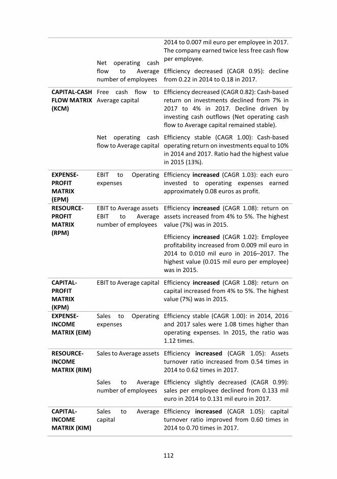
112

Net operating cash flow to Average number of employees

2014 to 0.007 mil euro per employee in 2017. The company earned twice less free cash flow per employee.

Efficiency decreased (CAGR 0.95): decline from 0.22 in 2014 to 0.18 in 2017.

CAPITAL-CASH FLOW MATRIX (KCM)

Free cash flow to Average capital

Net operating cash flow to Average capital

Efficiency decreased (CAGR 0.82): Cash-based return on investments declined from 7% in 2017 to 4% in 2017. Decline driven by investing cash outflows (Net operating cash flow to Average capital remained stable).

Efficiency stable (CAGR 1.00): Cash-based operating return on investments equal to 10% in 2014 and 2017. Ratio had the highest value in 2015 (13%).

EXPENSE-PROFIT MATRIX (EPM)

EBIT to Operating expenses

Efficiency increased (CAGR 1.03): each euro invested to operating expenses earned approximately 0.08 euros as profit.

RESOURCE-PROFIT MATRIX (RPM)

EBIT to Average assets EBIT to Average number of employees

Efficiency increased (CAGR 1.08): return on assets increased from 4% to 5%. The highest value (7%) was in 2015.

Efficiency increased (CAGR 1.02): Employee profitability increased from 0.009 mil euro in 2014 to 0.010 mil euro in 2016–2017. The highest value (0.015 mil euro per employee) was in 2015.

CAPITAL-PROFIT MATRIX (KPM)

EBIT to Average capital Efficiency increased (CAGR 1.08): return on capital increased from 4% to 5%. The highest value (7%) was in 2015.

EXPENSE-INCOME MATRIX (EIM)

Sales to Operating expenses

Efficiency stable (CAGR 1.00): in 2014, 2016 and 2017 sales were 1.08 times higher than operating expenses. In 2015, the ratio was 1.12 times.

RESOURCE-INCOME MATRIX (RIM)

Sales to Average assets

Sales to Average number of employees

Efficiency increased (CAGR 1.05): Assets turnover ratio increased from 0.54 times in 2014 to 0.62 times in 2017.

Efficiency slightly decreased (CAGR 0.99): sales per employee declined from 0.133 mil euro in 2014 to 0.131 mil euro in 2017.

CAPITAL-INCOME MATRIX (KIM)

Sales to Average capital

Efficiency increased (CAGR 1.05): capital turnover ratio improved from 0.60 times in 2014 to 0.70 times in 2017.

113

RESOURCE-EXPENSE MATRIX (REM)

Operating expenses to Average assets

Operating expenses to No of employees

Efficiency increased (CAGR 1.05): intensity of assets usage ratio has increased from 0.50 times in 2014 to 0.58 times in 2017.

Efficiency stable (CAGR 1.00): intensity of labour usage ratio has been stable at around 0.12 mil euro per employee throughout the period analysed.

CAPITAL-EXPENSE MATRIX (KEM)

Operating expenses to Average capital

Efficiency increased (CAGR 1.06): intensity of capital usage ratio increased from 0.55 times in 2014 to 0.65 times in 2017.

CAPITAL-RESOURCE MATRIX (KRM)

Average assets to Average capital

Average number of employees to Average capital

Efficiency stable (CAGR 1.00): average value of assets 1.12 times higher than average value of capital throughout the period analysed.

Efficiency increased (CAGR 1.06): average number of employees per 1 mil euro invested to capital increased from 4.50 to 5.36 employees.

Source: (by author).

Phase 2: Calculation and analysis of benchmark index of company’s overall efficiency (BICOE).

The author of the thesis adopts Tallink Grupp AS as the company to be analysed and Viking Line Abp as the company to be compared. Viking Line’s overall efficiency matrix is set out in Appendix 5 (Table 6). By using formula (2.46), comparative efficiency matrix (Table 2.9) for Tallink and Viking Line has been obtained.

114

Table 2.9. Comparative efficiency matrix of Tallink and Viking Line.

Source: (by author).

The benchmark indices of the overall efficiency of Tallink and Viking Line are presented in Table 2.10. This suggests that, while the companies’ overall efficiency levels were nearly equal in 2014, Tallink's efficiency level was higher than its competitor’s in the years that followed. The difference was biggest in 2017, when Tallink's overall efficiency level was 35% higher than Viking Line’s.

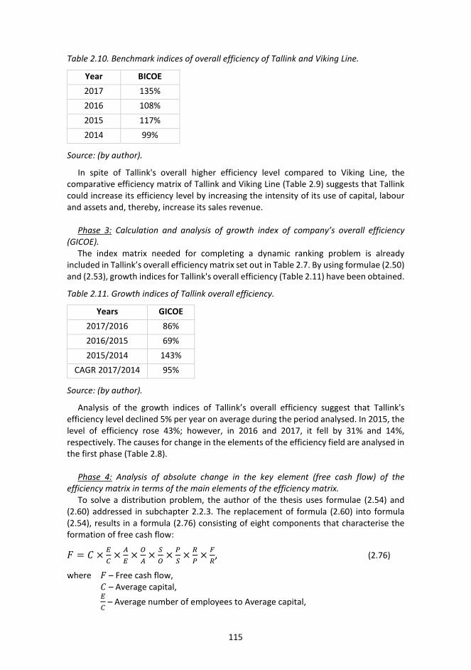
115

Table 2.10. Benchmark indices of overall efficiency of Tallink and Viking Line.

Year BICOE 2017 135% 2016 108% 2015 117% 2014 99%

Source: (by author).

In spite of Tallink's overall higher efficiency level compared to Viking Line, the comparative efficiency matrix of Tallink and Viking Line (Table 2.9) suggests that Tallink could increase its efficiency level by increasing the intensity of its use of capital, labour and assets and, thereby, increase its sales revenue.

Phase 3: Calculation and analysis of growth index of company’s overall efficiency (GICOE).

The index matrix needed for completing a dynamic ranking problem is already included in Tallink’s overall efficiency matrix set out in Table 2.7. By using formulae (2.50) and (2.53), growth indices for Tallink's overall efficiency (Table 2.11) have been obtained.

Table 2.11. Growth indices of Tallink overall efficiency.

Years GICOE 2017/2016 86% 2016/2015 69% 2015/2014 143%

CAGR 2017/2014 95%

Source: (by author).

Analysis of the growth indices of Tallink’s overall efficiency suggest that Tallink's efficiency level declined 5% per year on average during the period analysed. In 2015, the level of efficiency rose 43%; however, in 2016 and 2017, it fell by 31% and 14%, respectively. The causes for change in the elements of the efficiency field are analysed in the first phase (Table 2.8).

Phase 4: Analysis of absolute change in the key element (free cash flow) of the efficiency matrix in terms of the main elements of the efficiency matrix.

To solve a distribution problem, the author of the thesis uses formulae (2.54) and (2.60) addressed in subchapter 2.2.3. The replacement of formula (2.60) into formula (2.54), results in a formula (2.76) consisting of eight components that characterise the formation of free cash flow:

𝐹𝐹 = 𝐶𝐶 × 𝐸𝐸𝐶𝐶

× 𝐴𝐴𝐸𝐸

× 𝑂𝑂𝐴𝐴

× 𝑆𝑆𝑂𝑂

× 𝑃𝑃𝑆𝑆

× 𝑅𝑅𝑃𝑃

× 𝐹𝐹𝑅𝑅

, (2.76)

where 𝐹𝐹 – Free cash flow, 𝐶𝐶 – Average capital, 𝐸𝐸𝐶𝐶

– Average number of employees to Average capital,

116

𝐴𝐴𝐸𝐸

– Average assets to Average number of employees,𝑂𝑂𝐴𝐴

– Operating expenses to Average assets,𝑆𝑆𝑂𝑂

– Sales revenue to Operating expenses,𝑃𝑃𝑆𝑆

– EBIT to Sales revenue,𝑅𝑅𝑃𝑃

– Net operating cash flow to Profit,𝐹𝐹𝑅𝑅

– Free cash flow to Net operating cash flow.Table 2.12 sets out the value of every component in the component chain by year.

By using the chain-linking method (formulae 2.62 to 2.75), values for the conditional Free cash flow (F(Conditional)) may be obtained after the substitution of every component, the impact of every component on change in Free cash flow (∆F) and the impact of absolute change in every component on total change (%(∆F)).

Table 2.12. Distribution of absolute increment.

Source: (by author).

Based on Table 2.12, it may be concluded that in 2015 the increase in Free cash flow by 162 million euros was mainly due to:

− increase in Free cash flow to Net operating cash flow from 0.676 times to 1.376 times (absolute impact +134 million euros, impact on total change 83%),

− increase in EBIT to Sales revenue from 7.1% to 11.1% (absolute impact +60 million euros, impact on total change 37%),

− decrease of Net operating cash flow to Profit from 2.306 times to 1.818 times (absolute impact +35 million euros, impact on total change -21%).

In 2016, decline in free cash flow by 181 million euros was mainly caused by the same components that had increased this indicator in 2015:

− decrease of EBIT to Sales from 11.1% to 7.7% (absolute impact -80 million euros, impact on total change +44%),

− decrease of Free cash flow to Net operating cash flow from 1.376 times to 0.546 times (absolute impact -125 million euros, impact on total change +69%).

117

In 2017, free cash flow decreased by 33 million euros, which had two main drivers: − decrease of Net operating cash flow to Profit from 2.079 times to 1.828 times

(absolute impact -10 million euros), − decrease of Free cash flow to Net operating cash flow from 0.546 times to

0.363 times (absolute impact -25 million euros). The main conclusions can be summarised as follows:

− In 2014–2017, the biggest impact on the change (either increase or decrease) of absolute value of Free cash flow was due to the Free cash flow to Net operating cash flow indicator.

− In 2015 the increase in Free cash flow was mainly caused by one-off drivers (sale of three ships increased sales profitability as well Free cash flow to Net operating cash flow indicator).

− In 2016 the impact of one-off drivers from 2015 was offset. Additionally, two disproportions occurred: 1) Tallink was able to earn positive free cash flow of 27 million euros due to the increased average number of employees hired compared to capital employed but lost free cash flow of 25 million euros due to the lower average value of assets per employee; 2) Tallink was able to earn positive free cash flow of 20 million euros due to the increased intensity of assets usage but lost free cash flow of 10 million euros due to the lower Sales revenue to Operating expenses ratio. This means that the decrease in efficiency of labour and expense usage reduced free cash flow in 2016.

− In 2017 there were only indicators related to cash flow management affecting change (i.e. decrease) in free cash flow. A further six indicators had minor impact (less than +/- 10%). On the one hand, this demonstrates stability but, on the other hand, there were lost opportunities to increase free cash flow due to more efficient usage of capital, resources and expenses.

Phase 5: Indicate areas of efficiency improvement of the business activities of the company.

To give an overview of the status of each element of the efficiency field for all the years analysed, the author of the doctoral thesis created an efficiency improvement dashboard (Table 2.13). An efficiency improvement dashboard is a compound efficiency matrix (each element contains seven indicators) that shows the weaknesses compared to the main competitor (comparative coefficient indicated with “B-“) and the previous year (growth index indicated with “G-“). If the cell in the first column of the element is not filled in, it means that the value of efficiency field element of the company analysed is higher or equal than the competitor’s. If the cell in the second column of the element is empty, it means that the value of the efficiency field element of the company analysed has improved or is at the same level compared to the previous year.

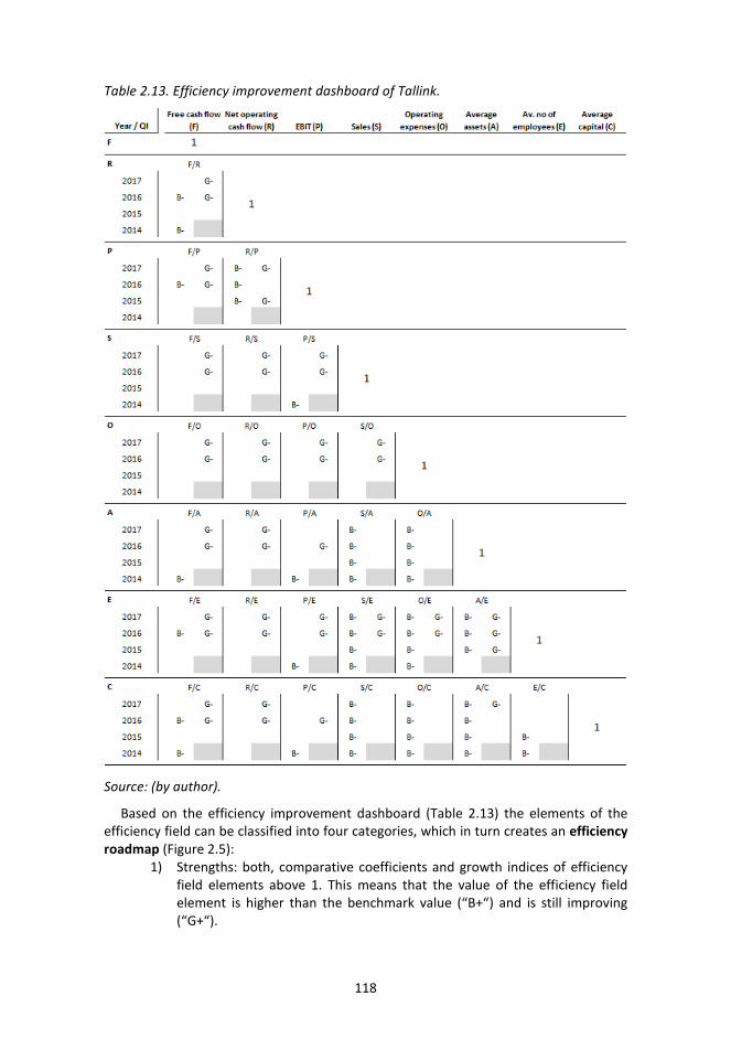
118

Table 2.13. Efficiency improvement dashboard of Tallink.

Source: (by author).

Based on the efficiency improvement dashboard (Table 2.13) the elements of the efficiency field can be classified into four categories, which in turn creates an efficiency roadmap (Figure 2.5):

1) Strengths: both, comparative coefficients and growth indices of efficiencyfield elements above 1. This means that the value of the efficiency fieldelement is higher than the benchmark value (“B+“) and is still improving(“G+“).

119

2) Improvements: comparative coefficients below 1, but growth indices ofefficiency field elements above 1. This means that the value of the efficiencyfield element is lower than the benchmark value (“B-“), but is improving(“G+“).

3) Setbacks: comparative coefficients above 1, but growth indices of efficiencyfield elements below 1. This means that the value of the efficiency fieldelement is higher than the benchmark value (“B+“), but is declining (“G-“).

4) Weaknesses: both, comparative coefficients and growth indices of efficiencyfield elements below 1. This means that the value of the efficiency fieldelement is lower than the benchmark value (“B-“) and is still declining(“G-“).

As it was concluded in the previous phases of this example, Tallink could increase its efficiency level compared to Viking Line by increasing the intensity of its use of capital, labour and assets and, thereby, increase its sales revenue. Compared to the previous, periods Tallink needs to pay attention to cash flow and profitability indicators.

Figure 2.5. Efficiency roadmap (based on Tallink 2017 data). Indicators marked with *-sign are the main elements of the efficiency field that reduced free cash flow (see Phase 4 for details). Source: (compiled by author).

As Figure 2.5 clearly demonstrates, there were only three efficiency field elements in the strengths category for Tallink in 2017. Hence, there are many recommended areas for Tallink to focus on when improving its efficiency:

− daily cash management (R/P, R/S, R/O, R/A, R/C), − labour usage (S/E, O/E, A/E, R/E, P/E), − capital management (e.g. usage of other sources financing, i.e. agreeing

longer payment terms with suppliers, A/C, S/C, O/C), − ensuring in the daily operations of the company that investments, which

resulted in a decrease in the efficiency level in 2017, contribute to a rise in the efficiency level in the coming years (otherwise the risk of overinvestment will materialise, F/R, F/P, F/S, F/O, F/A, F/E, F/C),

− expense management (R/O, P/O, S/O), − sales profitability (P/S), − assets usage (S/A, O/A).

120

As stated in subchapter 1.1, when improving efficiency, it is also essential to take into account the effectiveness of a company’s day-to-day operations, not just efficiency alone.

The author of the doctoral thesis believes that introducing an efficiency improvement dashboard and efficiency roadmap make the outcome of efficiency analysis more straightforward for end users (managers, analysts, etc.).

This subchapter illustrated the use of the overall efficiency matrix of a company using the example of an actually operating company. In using this approach, more comprehensive case studies and diagnostics can be performed using either publicly available or internal financial and non-financial data.

2.4 Further options for the use of an efficiency matrix 2.4.1 Adaptation of the company’s overall efficiency matrix based on the needs of users of financial statements The main users of financial statements are owners, minor investors, probable future investors, managers, creditors (banks and suppliers), customers, current and future employees, public institutions, professional associations, analysts, journalists and others.

Everybody performing matrix analysis may adapt the company’s overall efficiency matrix according to their needs. It is important to consider the ranking principle for initial indicators, and there has to be an even number of initial indicators if there is a desire to calculate overall efficiency indicators.

Below are some examples of the adaptation of the overall efficiency matrix of a company based on its user’s definition of the task:

1) The owner of a company wishes to analyse by components the formation offree cash flow remaining for their use in order to ascertain any potential freereserves. For this, the first component of the company’s overall efficiencymatrix has to be divided into two: owners’ equity and loan capital (financialliabilities), and free cash flow to equity may be adopted as the lastquantitative indicator. The rest of the initial indicators may be involved fromthe company’s overall efficiency matrix. Thus, a 10×10 efficiency matrix maybe developed, including, in order of finality:

- average equity, - average loan capital, - average number of employees, - average assets, - operating expenses, - sales revenue, - earnings before income tax and interest expenses, - net operating cash flow, - free cash flow (to firm), - free cash flow to equity.

The involvement of ten initial indicators results in the generation of 45 qualitative indicators, the comparison of which to competitors and previous periods makes it possible to ascertain the formation of remaining free cash flow and the reasons for change therein.

2) A retail investor considering the purchase of shares in a listed companywishes to analyse the formation of the exchange price of the share of thecompany it is interested in, based on the fundamental indicators of the

121

company. In this case, the exchange price of the share instead of free cash flow may be adopted as the last quantitative indicator. Thus, an 8×8 efficiency matrix is generated, including, in order of finality:

− average capital, − average number of employees, − average assets, − operating expenses, − sales revenue, − earnings before income tax and interest expenses, − net operating cash flow, − exchange price of the share (most recent).

By adopting as the benchmark the previous financial indicators of the same company and/or the indicators of its nearest competitors, it may be concluded based on 28 efficiency field elements whether change in the share price is due to change in the financial indicators of the company or, rather, some other factor (for example, the overall sentiment on the equity market).

3) The management of a company wishes to compare the efficiency of itscompany to that of its nearest competitor. In this case, it pays to analyse ingreater detail the expense indicators of assets and of an income statementin an efficiency matrix. We assume that the two biggest asset groups of acompany are tangible fixed assets and accounts receivable and that its twobiggest expense groups are cost of materials and labour expenses. Based onsubchapter 2.1, asset and expense groups have to be ranked into anefficiency matrix in the order of their decreasing share in the balance sheetand income statement structure. Thus, a 10×10 efficiency matrix isgenerated, including, in order of finality:

− average capital, − average number of employees, − average tangible fixed assets, − average accounts receivable, − cost of materials, − labour expenses, − sales revenue, − earnings before income tax and interest expenses, − net operating cash flow, − free cash flow (to firm).

The involvement of ten initial indicators results in the generation of 45 qualitative indicators in an efficiency field, the comparison of which to the nearest competitor and previous periods of one’s own company makes it possible to ascertain in detail what the strengths and weaknesses of the company analysed are compared to its nearest competitor and previous periods. In the estimation of the author of the thesis, this is a sufficient quantity of data in order to identify hidden reserves and develop an action plan to raise the efficiency level of a company.

4) Industry association aims to analyse efficiency using an industry-specificoverall efficiency matrix. In this case, at first, factor analysis can be used to

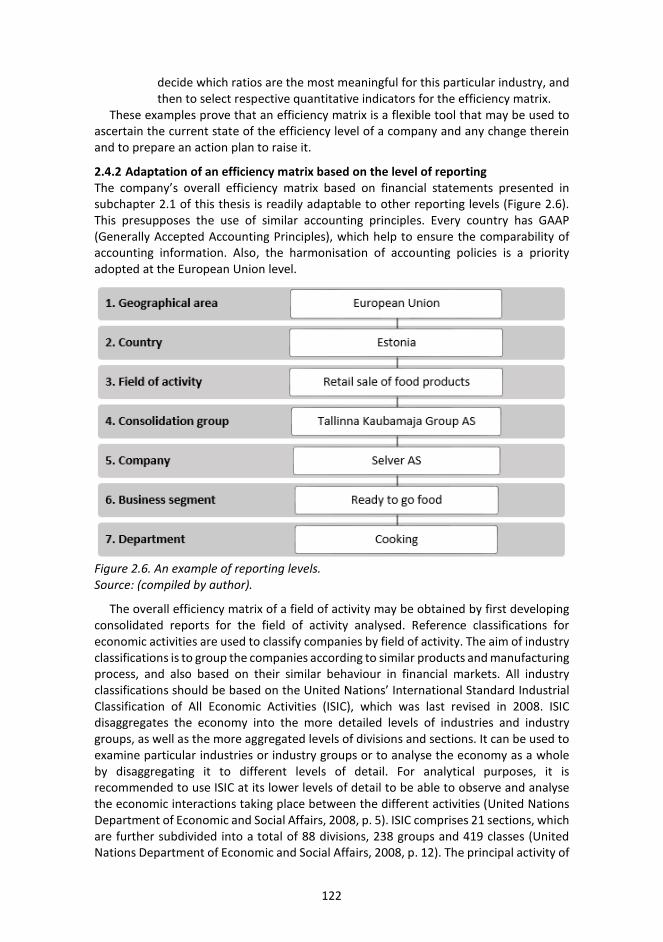
122

decide which ratios are the most meaningful for this particular industry, and then to select respective quantitative indicators for the efficiency matrix.

These examples prove that an efficiency matrix is a flexible tool that may be used to ascertain the current state of the efficiency level of a company and any change therein and to prepare an action plan to raise it.

2.4.2 Adaptation of an efficiency matrix based on the level of reporting The company’s overall efficiency matrix based on financial statements presented in subchapter 2.1 of this thesis is readily adaptable to other reporting levels (Figure 2.6). This presupposes the use of similar accounting principles. Every country has GAAP (Generally Accepted Accounting Principles), which help to ensure the comparability of accounting information. Also, the harmonisation of accounting policies is a priority adopted at the European Union level.

Figure 2.6. An example of reporting levels. Source: (compiled by author).

The overall efficiency matrix of a field of activity may be obtained by first developing consolidated reports for the field of activity analysed. Reference classifications for economic activities are used to classify companies by field of activity. The aim of industry classifications is to group the companies according to similar products and manufacturing process, and also based on their similar behaviour in financial markets. All industry classifications should be based on the United Nations’ International Standard Industrial Classification of All Economic Activities (ISIC), which was last revised in 2008. ISIC disaggregates the economy into the more detailed levels of industries and industry groups, as well as the more aggregated levels of divisions and sections. It can be used to examine particular industries or industry groups or to analyse the economy as a whole by disaggregating it to different levels of detail. For analytical purposes, it is recommended to use ISIC at its lower levels of detail to be able to observe and analyse the economic interactions taking place between the different activities (United Nations Department of Economic and Social Affairs, 2008, p. 5). ISIC comprises 21 sections, which are further subdivided into a total of 88 divisions, 238 groups and 419 classes (United Nations Department of Economic and Social Affairs, 2008, p. 12). The principal activity of

123

a company is the activity that contributes most to the value added of the company (United Nations Department of Economic and Social Affairs, 2008, p. 13).

In the European Community, Statistical Classification of Economic Activities (NACE) is used. Similar to ISIC, NACE contains 21 sections, which are subdivided into 88 divisions. Further down, NACE consists of 272 groups and 615 classes (Eurostat, 2008, p. 48).

The Estonian classification of economic activities (EMTAK) follows the European NACE classification but it has also introduced a fifth level of subdivision by establishing 775 sub-classes (Eesti Statistikaamet, 2008). Based on the UN questionnaire conducted in 2013, at least 117 countries have introduced own classification of economic activities (United Nations, Department of Economic and Social Affairs, Statistics Division, 2018).

The use of an efficiency matrix at the level of the consolidation group provides the management of a company with the option of comparing the efficiency matrix of every company in the group to the group’s efficiency matrix and to understand at which company in the group and to which aspects of the operations to devote more attention. Since the financial reporting of a consolidation group has to be done according to the same accounting principles, companies located in different countries may also be compared using the efficiency matrix.

Since there may be several business segments within the same company, it is important to understand what impact every segment has on the level of efficiency of the company. By analysing an efficiency matrix, in the future the entrepreneur will find out precisely what the strengths and weaknesses of every segment are compared to the aggregate indicators or other segments of the company. At companies where several departments are linked to the same business segment, an efficiency matrix may be used to carry out a comparative analysis of the efficiency levels of the departments and take specific measures to raise the efficiency.

It is important to consider that information gathered at company and group levels may also be used at higher levels without gathering additional data. Countries (for example, Estonia) where the automated collection of financial statements is used have created the preconditions for the creation of an efficient automated comparative analysis system at the levels of both the field of activity and the country.

At every level of analysis, multiple comparison bases may be used (Table 2.14). If the precondition of the comparability of information has been met, efficiency matrices may be compared at the levels of geographic region, country and field of activity to efficiency matrices of another geographic region, country and field of activity or any previous year. Ranking lists of companies may be developed both in terms of fields of activity and regions as well as at country level. The list of ranking makes it possible for every entrepreneur to have a systematised and objective picture of the developments in his/her sector or region and to position himself/herself against other (competing) entrepreneurs. Furthermore, information about current and potential business partners (including clients and suppliers) may be obtained from ranking lists of companies.

At the levels of the group, company, operating segment and department, in addition, efficiency matrices for any previous quarter or month may be used as the benchmark. Since, as a rule, entrepreneurs are required to publish annual reports once a year, efficiency matrices may be compared in terms of years based on publicly available data. Listed companies are an exception, as they disclose their financial results every three months. In the case of monthly and quarterly comparisons, it makes sense, for better comparability, to use as the comparison basis financial information from the immediately preceding quarter or month or from the same quarter or month of the previous year.

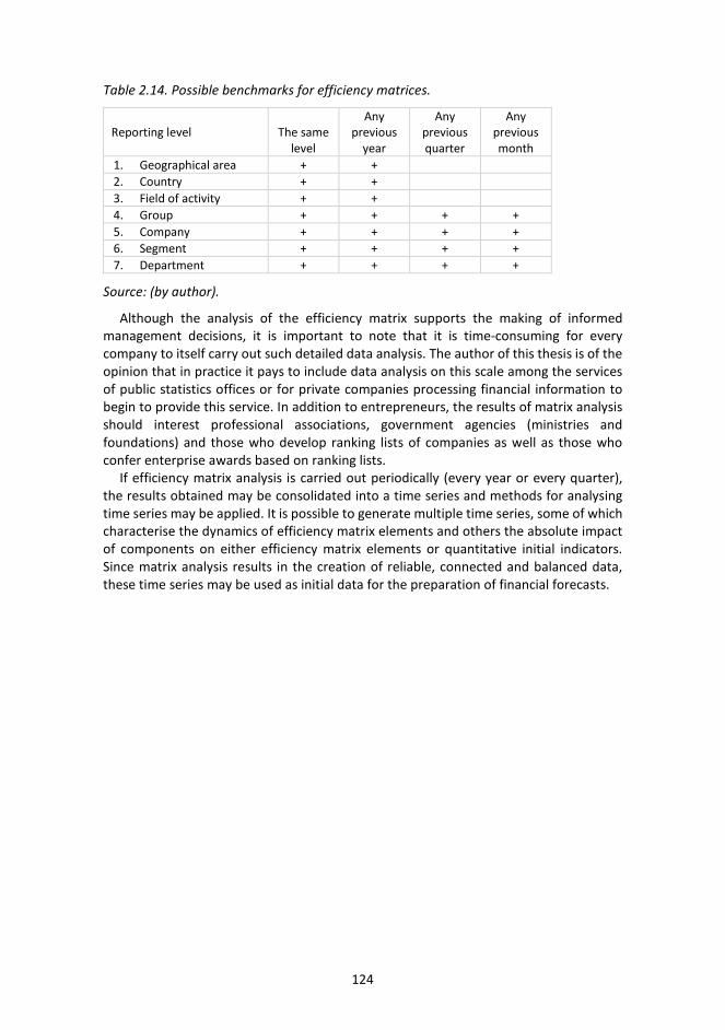
124

Table 2.14. Possible benchmarks for efficiency matrices.

Reporting level The same level

Any previous

year

Any previous quarter

Any previous month

1. Geographical area + + 2. Country + + 3. Field of activity + + 4. Group + + + + 5. Company + + + + 6. Segment + + + + 7. Department + + + +

Source: (by author).

Although the analysis of the efficiency matrix supports the making of informed management decisions, it is important to note that it is time-consuming for every company to itself carry out such detailed data analysis. The author of this thesis is of the opinion that in practice it pays to include data analysis on this scale among the services of public statistics offices or for private companies processing financial information to begin to provide this service. In addition to entrepreneurs, the results of matrix analysis should interest professional associations, government agencies (ministries and foundations) and those who develop ranking lists of companies as well as those who confer enterprise awards based on ranking lists.

If efficiency matrix analysis is carried out periodically (every year or every quarter), the results obtained may be consolidated into a time series and methods for analysing time series may be applied. It is possible to generate multiple time series, some of which characterise the dynamics of efficiency matrix elements and others the absolute impact of components on either efficiency matrix elements or quantitative initial indicators. Since matrix analysis results in the creation of reliable, connected and balanced data, these time series may be used as initial data for the preparation of financial forecasts.

125

Conclusion The efficiency growth of companies’ economic activities plays a significant role in the growth of gross domestic product, and it also exerts a positive effect on the social development of society. The research problem addressed in the doctoral thesis is that the level of efficiency of a company cannot be evaluated based on a single financial ratio; however, ranking companies according to their efficiency levels on the basis of multiple indicators is complicated. Usually, financial ratios are considered as distinct when calculated or interpreted. This thesis has reached the conclusion that it is expedient to solve separately the tasks of evaluating the level of efficiency and of ranking companies. In this case, it is possible both to analyse the formation of the efficiency level of a company and to compare its efficiency level to the indicators of other companies or of the same company for previous periods.

The main objective of this doctoral thesis was to demonstrate that today, using publicly available financial information, the efficiency level of a company and change therein may be measured based on an efficiency matrix. The efficiency matrix concept, described by the Estonian academician Uno Mereste for the first time in 1977, was well known in Estonia and Russia from the 1970s to the 1990s and, to a lesser extent, in the 2000s.

As a result of the solution of seven research tasks defined for the accomplishment of the objective of the doctoral thesis, several important conclusions and results, summarised below, were reached.

Task 1: Investigate the development of efficiency analysis to date. The doctoral thesis demonstrates that in recent decades many methodologies have

been developed for the calculation and analysis of both efficiency and of change therein. The first and best known study on the evaluation of efficiency may be considered the paper published by Cobb and Douglas in 1928, which considered the production function. Up to the 1970s, research predominantly focused on the evaluation of the efficiency of production; subsequently, the efficiency of all business activities began to be studied more. Research concerning efficiency has utilised various parametric and non-parametric methods: production, revenue, cost and profit functions, index and stochastic frontier models, data envelopment analysis, Bayesian techniques, balanced scorecard, fuzzy multiple criteria decision making, fuzzy analytical hierararchy process etc. Several authors concluded that the choice of method used for the efficiency analysis could make a meaningful effect on the conclusions of an efficiency study. Many authors were convinced that efficiency needs to be broken down into its components, so that it is easier to analyse efficiency and the formation thereof.

Task 2: Investigate in greater depth the development of matrix modelling and of the concept of the efficiency matrix to date.

The predecessor of the efficiency matrix may be considered to be the complex analysis methodology published by Professor Anatoli Sheremet of the Moscow State University in 1974. Based on that, the order of the performance of complex analysis (Sheremet proposed 13 stages) and benchmarks underlying evaluations were important. Estonian academician Uno Mereste supplemented complex analysis with the principle of systemicity, since comprised within the concept of a system is the requirement of integrity, which a complex need not include.

In order to distinguish the complex analysis methodology begun by Sheremet and the supplementations created by Mereste, the latter is referred to as system integrated

126

analysis. Since system integrated analysis is based on the theory of index numbers, it is limited by the fact that it can be used to investigate only those economic factors that appear as multiples of a performance indicator. This suggests that the use of statistical analysis in the creation of an efficiency matrix is not necessary or possible. The reason for no need is that the purpose of qualitative indicators in an efficiency matrix is to show the binding nature of two quantitative indicators (that is, how many indicator units in the numerator there are per unit in the denominator) but not a relationship (the latter shows how much a dependent variable changes in the event of the argument changing by one unit) between these indicators. The financial indicators for one company for one period are sufficient to develop an efficiency matrix; however, the ascertainment of the shape of the relationship and the statistical analysis of parameters require financial information from a greater number of either companies or periods. This means that system integrated analysis may be used, for example, to explain how profit is affected by change in the number of employees, the cost of non-current assets and sales revenue. At the same time, system integrated analysis cannot be used to analyse the impact of training events, employee motivation, management culture and other affects on change in profit.

Based on the study conducted as part of this thesis, the author of this doctoral thesis split the development of the efficiency matrix concept into four periods and provided an overview of the pioneering and most considerable research published in these periods.

1) 1976–1981: Formation of the visual form of an efficiency matrix,− 1976: Development of the methodology of economic analysis was included

among the major research areas of the Tallinn Polytechnic Institute (TPI) − 1977: Professor Mereste presented for the first time the principles of the matrix

approach to the economic efficiency of manufacturing developed at the Faculty of Economics of the Tallinn Polytechnic Institute.

− 1980: Mereste was the first to present an efficiency matrix in visual form, developing a 6х6 efficiency matrix for the national economy.

− 1981: Mereste presented a structured efficiency matrix, consolidating under the main diagonal all those elements that should increase as efficiency rises on the assumption that all the other indicators remain the same.

2) 1980–1984: Composition of overall efficiency indicators,− 1980: Mereste defined the need for solving a dynamic ranking problem, and

proposed a formula for calculating an overall efficiency index (arithmetic mean of the growth indices of the elements of an efficiency field).

− 1981: Mereste defined the need for solving a static ranking problem, and proposed a formula for calculating an overall comparative multiplier of efficiency (arithmetic mean of the benchmark indices of the elements of the efficiency fields of the companies compared).

− 1981: Andres Root pointed out that, since indices characterising change in efficiency are multiples, it is more appropriate to calculate an overall efficiency index as the geometric mean of the growth indices of the elements of an efficiency field.

− 1984: Vello Vensel presented an economic efficiency vector of manufacturing (efficiency vector indicator) based on the concept of the efficiency matrix.

3) 1984–1990: Rapid development of the concept of efficiency matrix− 1984: Mereste provided information about the concept of an efficiency field

(level of economic efficiency).

127

− 1984: Mereste defined the problem of the distribution of the absolute increment, proposing the use of the chain-linking method as a solution.

− 1985: Vensel constructed a 7х7 efficiency matrix for the investigation of the efficiency of labour. Vensel emphasised that all the elements of an efficiency matrix are interlinked and demonstrated how to analyse change in the value of the elements in the first column of an efficiency matrix by components.

− 1985: Toomas Rammo and Vello Volt presented a 10х10 efficiency matrix for manufacturing activities and provided information about its division into three submatrices (efficiency matrices for the use of labour as well as current and non-current assets).

− 1986: Vello Volt and Rein Volt supplemented Vensel’s 1985 study with the nuance that change in the values of all the elements of an efficiency matrix can be analysed by components.

− 1986: Vello Volt and Raul Renter clarified the order of the replacement of the components affecting the indicator investigated when the problem of the distribution of the absolute increment is solved.

− 1987: Jaan Alver and Vello Järve presented their study of the efficiency of retail stores (earlier studies focused on manufacturing companies).

− 1987: Root compiled an efficiency matrix to analyse the dynamics and fulfilment of the plan (budget).

− 1988: Maimu Saarepera presented bases for grouping matrix models according to the principle of the involvement of quantitative indicators in a matrix, the location of source information and the number of indicators in every element of a matrix model.

− 1988: Saarepera presented a modified matrix model in which initial information is placed on the main diagonal and a concentric matrix model in which the object of investigation is two quantitative variables interlinked in a relationship of the cause-and-effect type.

− 1988: based on efficiency matrices, Vensel developed a composite evaluation model for the economic activities of a company.

− 1988: Alver divided the quantitative input indicators of an efficiency matrix into two groups: resource and expense indicators.

− 1989: Alver and Järve published a 9×9 matrix model of retail stores’ key indicators and introduced six areas in the efficiency matrix that could be analysed independently.

− 1990: Luur presented a matrix model of the dynamics of the economic efficiency of export and import activities of 12 developed capitalist countries between 1960 and 1985.

4) 2000–today: Rebirth of efficiency matrix concept− 2001: Vensel presented a 7х7 efficiency matrix to analyse the performance of

Estonian commercial banks. − 2007: Eedo Kalle published an index matrix for evaluation of productivity level. − 2011: Startseva, Alver and Siimann published the first English-language review

papers about the methodology of matrix-based analysis. − 2015: Siimann and Alver used an efficiency matrix to analyse changes in profit

per employee using the example of Estonia’s small and medium-sized IT and telecommunications companies from 2009 to 2013.

128

− 2016: The doctoral thesis defended by Startseva created an efficiency matrix based on the internal data of companies and used it to enhance processes.

Task 3: Ascertain which financial ratios have been used most in research to date and what their applicability is in the analysis of an efficiency matrix.

Discussions about determining the most efficacious group of ratios started in the 1920s. Based on the methodology used, the classifications can be divided into empirical (created according to author’s experience), deductive (created using technical relationships between ratios) and inductive (statistical techniques are used to classify financial ratios) approaches. Compilation of the efficiency matrix is somewhat similar to the deductive classification, where technical relationships are used for ratio classification.

The research demonstrated that despite the classification methodology, there is only consensus about the most commonly used ratio categories, such as profitability and liquidity, but other ratio categories differed across studies. It was also concluded that factor analysis has mainly been used to classify ratios using statistical methods. Hence, factor analysis can be used to decide which ratios are the most meaningful to explain the financial data chosen by the analyst and to bear this in mind when selecting quantitative indicators for the efficiency matrix.

It was concluded that liquidity, solvency, efficiency of assets usage, investment profitability and assets structure ratios have mainly been covered by well-known financial ratios. Sales profitability, the efficiency of labour usage, cost efficiency and earnings quality are the main examples of business aspects poorly covered by popular financial ratios. The results supported the actuality of the research problem of this doctoral thesis in that there is a clear need for a tool to support comprehensive efficiency analysis.

Task 4: Provide a company’s overall efficiency matrix encompassing the various facets of business activities. For this, both the selection of quantitative initial indicators and the order in which they are involved in an efficiency matrix are important.

In order to ensure that business activities are reflected comprehensively, the author of this thesis increased the number of the groups of financial indicators involved in the efficiency matrix from the previous three to six, also including a capital group, and divided performance indicators into income, profit and cash flow indicators.

As part of this thesis, a company’s overall efficiency matrix was constructed, involving eight quantitative indicators: average capital for the period, average number of employees for the period, average assets for the period, operating expenses, sales revenue, EBIT, net operating cash flow and free cash flow.

The company’s overall efficiency matrix is based on the following assumptions: 1) only information contained in publicly available annual reports is used,2) consideration is given to the order in which quantitative indicators are involved

in the matrix model: raising capital makes it possible to invest in resources that,through expenses, are transformed into income, profit and cash flow,

3) financial information readily comparable between companies is used,4) a matrix model involves an even number of quantitative indicators, thereby

enabling dynamic analysis and comparative analysis of efficiency levels in amanner where the result of the analysis is affected by all the quantitativeindicators.

129

Unlike previous research, the company’s overall efficiency matrix places greater emphasises on the importance of analysing cash-based financial indicators, as a result of which net operating cash flow and free cash flow are involved in the matrix.

Task 5: Ascertain how to analyse relationships between the elements of an efficiency matrix and measure the mutual impacts thereof.

Involving at least two quantitative indicators from each of the six groups of financial indicators, 21 submatrices will be created under the main diagonal of the efficiency matrix (in the efficiency field), all of which can be analysed separately. Based on the company’s overall efficiency matrix, 17 submatrices are created.

Every quantitative indicator may be considered in two ways: as a component having an impact (presented in the first column of the efficiency matrix) and as a performance indicator (presented in the first row). The thesis demonstrated that the formation of each quantitative initial indicator can be analysed by means of another quantitative indicator and, depending on the research task, one or several qualitative indicators.

Of the relationships between the elements of an efficiency matrix, the relationship between the key element of an efficiency field and the main elements of an efficiency field is considered the most important. Since all the elements of an efficiency matrix are interlinked, the thesis has provided specific instructions on the creation of these relationships. The thesis demonstrates that the chain-linking method can be used to distribute the absolute increase of an indicator analysed among the components that have affected it.

Task 6: Propose overall efficiency indicators for the evaluation of efficiency levels and of change therein.

The author of the thesis proposed two overall efficiency indicators: 1) benchmark index of company’s overall efficiency (BICOE), which may be used

to determine unused internal reserves at a company and to rank companiesbased on the level of efficiency;

2) growth index of company’s overall efficiency (GICOE), which can be used toanalyse change in the level of efficiency and to rank companies based onchange in the level of efficiency.

Both overall efficiency indicators have a practical value for entrepreneurs interested in increasing the efficiency of their companies and people developing ranking lists based on the financial information of companies, since both indicators are developed on the principle of full systemicity.

Task 7: Demonstrate options for the use of an efficiency matrix and developments thereof at the level of the company.

Based on the financial indicators of an actual company (Tallink Grupp), the author of the doctoral thesis created a numerical example of the company’s overall efficiency matrix, analysed the level of efficiency by comparison to the nearest competitor (Viking Line) and the previous period and used the chain-linking method for the ascertainment of the reasons for change in the value of the key element of the efficiency field (free cash flow). To make the outcome of efficiency analysis more straightforward for end users (managers, analysts, etc.), the author of this thesis introduced an efficiency improvement dashboard and efficiency roadmap. Based on the calculations, proposals are made as to which efficiency field indicators a company should focus on, increasing their values in order to raise its level of efficiency going forward.

The main advantages of the usage of the efficiency matrix considered in this thesis:

130

− its systemicity (that is, its ability to involve various facets of business activities in one model),

− simplicity of the creation of an efficiency matrix (workability with a small quantity of initial data readily found in annual reports);

− possibilities for developing an efficiency matrix (ascertainment of the absolute variance of every component that has affected the level of efficiency; calculation of overall efficiency indices).

The scientific contribution made by the author of this doctoral thesis may be briefly summarised as follows:

1) The development of complex analysis and system integrated analysis to datehas been investigated in greater depth. The results obtained were presentedfor the first time in English scientific literature with a profile of key researchbased on complex analysis and system integrated analysis.

2) It was ascertained how financial ratios have been classified in previousresearch and what kinds of financial ratios have been used most in research.

3) In analysing the level of efficiency, the company’s overall efficiency matrixbased on eight quantitative indicators, which is easy to develop based onpublicly available annual reports, has been proposed. The rule on theinvolvement of initial indicators in an efficiency matrix was updated bydividing financial indicators into six groups (capital, resource, expense,income, profit and cash flow indicators). The efficiency field of the company’soverall efficiency matrix has been split into 17 submatrices and 28 qualitative indicators, which can all be analysed individually.

4) Two overall efficiency indicators (benchmark index of company’s overallefficiency and growth index of company’s overall efficiency) have beenconstructed and may be used for ranking companies (developing rankinglists) based on the efficiency levels of companies and on change therein.

5) Computing rules have been developed to ascertain the impact of a specificelement (or elements) of an efficiency matrix on another specific element.

6) A methodology based on the chain-linking method has been proposed fordividing the absolute increment of the analysed indicator between thecomponents that have affected it.

7) In addition to company’s overall efficiency matrix, an efficiency improvement dashboard and an efficiency roadmap were introduced to make theefficiency analysis more straightforward for the users.

8) It has been demonstrated that matrix modelling based on the efficiency fieldconcept is a universal and flexible approach to analysing efficiency levels andchange therein and that it may be applied at all management levels (from the level of the department to geographical regions).

The results of the doctoral thesis can be developed: 1) by creating specific efficiency matrices for companies and fields of activity

based on information in annual reports according to the needs of differentusers of financial information, using for it the principles for the constructionof an efficiency matrix as presented in this thesis;

2) by testing the workability of the company’s overall efficiency matrix at thelevel of the country and by developing this, introducing two-level analysis,which also makes it possible to analyse the impact of structural shifts on

131

aggregate change in the overall efficiency level of a company at the level of the country;

3) by further developing the composite evaluation model for the economicactivities of a company, developed by Vensel in 1988, based on thecompany’s overall efficiency matrix proposed in this thesis;

4) by testing the creation of an overall efficiency matrix for a field of activity and by using initial data ascertained from factor analysis and quantitativeindicators derived from the key ratios of every factor;

5) by investigating in detail the components that affect the formation of andchange in the qualitative indicators of an efficiency field (for example, impact of the work environment on labour productivity, impact of themanufacturing process on Sales revenue to Assets and the like);

6) by analysing the values of efficiency matrix elements as time series, usingstatistical and econometric methods for this.

This doctoral thesis made both a theoretical and empirical contribution to introducing the use of the efficiency matrix and its developments. The author of the thesis hopes that readers have come away with an idea of what rich and multi-faceted analytical information may be obtained from efficiency matrices and that it will convince both managers and financial analysts of the expediency of using matrix models in the future.

132

List of Figures Figure 1.1. Conceptual framework of efficiency. ............................................................ 12 Figure 1.2. Efficiency and effectiveness. ......................................................................... 13 Figure 1.3. Financial ratios categorical framework. ........................................................ 20 Figure 1.4. An example of “Pyramid of ratios” approach. .............................................. 21 Figure 1.5. Formation and investigation of main indicator groups in a complex analysis system according to A. Sheremet. .................................................................................. 33 Figure 1.6. A complex of relationships whereby a full complex analysis of labour and machine work efficiency is secured includes, besides these two indicators, a further four qualitative indicators are linked to the same quantitative results. ................................ 36 Figure 1.7. An example of the efficiency field including 20 qualitative indicators (arrows pointed upwards from financial ratio numerator to denominator) surrounded by five quantitative initial parameters. ...................................................................................... 47 Figure 1.8. Summary of matrix modelling and developments thereof. .......................... 60 Figure 1.9. Usage of efficiency matrix linked to financial statement analysis (FSA). ...... 62 Figure 2.1. Division of efficiency field into three submatrices. ....................................... 69 Figure 2.2. Division of efficiency field into six submatrices. ........................................... 70 Figure 2.3. Classification of quantitative indicators. ....................................................... 72 Figure 2.4. Division of efficiency field into 21 submatrices............................................. 74 Figure 2.5. Efficiency roadmap (based on Tallink 2017 data). ...................................... 119 Figure 2.6. An example of reporting levels. .................................................................. 122

133

List of Tables Table 1.1. Financial ratios selected to represent each factor. ........................................ 24 Table 1.2. Principle components and the financial ratios representing the best every component. ..................................................................................................................... 24 Table 1.3. Number of papers split by periods. ................................................................ 27 Table 1.4. Financial ratios ranked according to popularity in scientific literature. ......... 27 Table 1.5. Number of popular ratios split by categories. ................................................ 30 Table 1.6. General form of an efficiency matrix.............................................................. 39 Table 1.7. Efficiency matrix of national economy. .......................................................... 40 Table 1.8. Structured efficiency matrix of a machine factory or shipyard. ..................... 41 Table 1.9. General form of an index matrix. ................................................................... 42 Table 1.10. An example of modified matrix model. ........................................................ 51 Table 1.11. Example of concentric matrix model. ........................................................... 52 Table 1.12. An example of a retail store efficiency matrix.............................................. 53 Table 1.13. Efficiency matrix of retail stores’ performance. ........................................... 54 Table 1.14. Index matrix for the evaluation of productivity level. .................................. 57 Table 1.15. Efficiency matrix for change in profit per employee analysis. ..................... 58 Table 2.1. List of quantitative indicators published in annual reports. ........................... 78 Table 2.2. The company’s overall efficiency matrix. ....................................................... 82 Table 2.3. Interpretation of the efficiency field elements of company’s overall efficiency matrix. ............................................................................................................................. 85 Table 2.4. Efficiency matrix of comparative coefficients (based on company’s overall efficiency matrix) ............................................................................................................ 99 Table 2.5. Index matrix (based on company’s overall efficiency matrix) ...................... 101 Table 2.6. Initial data and their dynamics for compilation of Tallink’s overall efficiency matrix. ........................................................................................................................... 107 Table 2.7. Overall efficiency matrix of Tallink. .............................................................. 109 Table 2.8. Analysis of the efficiency field elements of Tallink’s overall efficiency matrix. . 110 Table 2.9. Comparative efficiency matrix of Tallink and Viking Line. ............................ 114 Table 2.10. Benchmark indices of overall efficiency of Tallink and Viking Line. ........... 115 Table 2.11. Growth indices of Tallink overall efficiency. ............................................... 115 Table 2.12. Distribution of absolute increment. ........................................................... 116 Table 2.13. Efficiency improvement dashboard of Tallink. ........................................... 118 Table 2.14. Possible benchmarks for efficiency matrices. ............................................ 124

134

References Aigner, D., Lovell, C. K., & Schmidt, P. (1977). Formulation and estimation of stochastic

frontier production function models. Journal of econometrics, 6(1), 21–37. Altman, E. I. (1968). Financial ratios, discriminant analysis and the prediction of corporate

bankruptcy. The Journal of Finance, 23(4), 589–609. Alver, J. (1988). Lähteandmete järjestamine ja efektiivsuse osaindeksid sidusanalüüsis.

Infotehnoloogia ja täppismajandusteadus (pp. 247–252). Tallinn: Eesti Majandusteaduse Selts.

Alver, J., & Alver, L. (2011). Majandusarvestus ja rahandus I. Tallinn: Deebet. Alver, J., & Järve, V. (1987). Kooperatiivide töötulemuste sidusanalüüsist. Nõukogude

Eesti Kooperaator, 2(107), 25–26. Alver, J., & Järve, V. (1989). Kooperatiivide kaubandustegevuse efektiivsuse kompleksne

võrdlevanalüüs. Nõukogude Eesti Kooperaator, 2(115), 26–31. Amit, R., & Livnat, J. (1990). Grouping of conglomerates by their segments economic

attributes: towards a more meaningful ratio analysis. Journal of Business Finance & Accounting, 17(1), 85–100.

Asmild, M., Paradi, J. C., Reese, D. N., & Tam, F. (2007). Measuring overall efficiency and effectiveness using DEA. European Journal of Operational Research, 178(1), 305–321.

Bahiraie, A., Ibrahim, N. A., & Azhar, A. M. (2011). Genetic programming approach for testing credit risk box method. Scientific Research and Essays, 6(17), 3584–3594.

Banker, R. D., Charnes, A., & Cooper, W. W. (1984). Some models for estimating technical and scale inefficiencies in data envelopment analysis. Management science, 30(9), 1078–1092.

Barnes, P. (1982). Methodological implications of non-normally distributed financial ratios. Journal of Business Finance and Accounting, 9(1), 51–62.

Barnes, P. (1987). The analysis and use of financial ratios: a review article. Journal of Business Finance and Accounting, 14(4), 449–461.

Battese, G. E., & Corra, G. S. (1977). Estimation of a production frontier model: with application to the pastoral zone of Eastern Australia. Australian journal of agricultural economics, 21(3), 169–179.

Beaney, M. (2014, March 19). Analysis. Retrieved from The Stanford Encyclopedia of Philosophy: https://plato.stanford.edu/entries/analysis/

Beaver, W. H. (1966). Financial ratios as predictors of failure. Journal of Accounting Research, 4 (Empirical Research in Accounting: Selected Studies 1966), 71–111.

Beaver, W. H., McNichols, M. F., & Rhie, J. W. (2005). Have financial statements become less informative? Evidence from the ability of financial ratios to predict bankruptcy. Review of Accounting studies, 10(1), 93–122.

Berry, R. H., & Nix, S. (1991). Regression analysis v. ratios in the cross-section analysis of financial statements. Accounting and Business Research, 21(82), 107–117.

Bird, R. G., & McHugh, A. J. (1977). Financial ratios — an empirical study. Journal of Business Finance & Accounting, 4(1), 29–46.

Bjurek, H., Hjalmarsson, L., & Forsund, F. R. (1990). Deterministic parametric and nonparametric estimation of efficiency in service production: a comparison. Journal of Econometrics, 46(1–2), 213–227.

Blackburn, S. (2016). The Oxford Dictionary of Philosophy. Oxford: Oxford University Press.

135

Blum, M. (1974). Failing company discriminant analysis. Journal of Accounting Research, 13, 1–25.

Bodie, Z., Kane, A., & Marcus, A. J. (2004). Essentials of Investments (5 ed.). McGraw-Hill Irwin.

Bougen, P. D., & Drury, J. C. (1980). UK statistical distributions of financial ratios, 1975. Journal of Business Finance & Accounting, 7(1), 39–47.

Buijink, W., & Jegers, M. (1986). Cross-sectional distributional properties of financial ratios in Belgian manufacturing industries: aggregation effects and persistence over time. Journal of Business Finance and Accounting, 13(3), 337–363.

Cambridge University Press. (2018, June 29). Efficiency. Retrieved from Cambridge Dictionary: https://dictionary.cambridge.org/dictionary/english/efficiency

Cannon, D. M. (2002). Contaminated distributions: a new perspective on the financial ratio non-normality problem. Kent: Kent State University.

Carlino, L., Coppens, F., González, J., Ortega, M., Pérez-Duarte, S., Rubbrecht, I., & Vennix, S. (2017). Statistics Paper Series: Decomposition techniques for financial ratios of European non-financial listed groups (Vol. 21). Frankfurt: European Cental Bank.

Casey, C., & Bartczak, N. (1985). Using operating cash flow data to predict financial distress: Some extensions. Journal of Accounting Research, 23(1), 384–401.

Caves, D., Christensen, L., & Diewert, E. (1982). The economic theory of index numbers and the measurement of input, output, and productivity. Econometrica, 50(6), 1393–1414.

Chakraborty, K., Biswas, B., & Lewis, W. C. (2001). Measurement of technical efficiency in public education: a stochastic and nonstochastic production function approach. Southern Economic Journal, 67(4), 889–905.

Chakravarthy, B. S. (1986). Measuring strategic performance. Strategic Management Journal, 7(5), 437–458.

Chan, F. T. (2003). Performance measurement in a supply chain. The International Journal of Advanced Manufacturing Technology, 21(7), 534–548.

Charnes, A., Cooper, W. W., & Rhodes, E. (1978). Measuring the efficiency of decision making units. European journal of operational research, 2(6), 429–444.

Charnes, A., Cooper, W. W., & Rhodes, E. (1981). Evaluating program and managerial efficiency: an application of data envelopment analysis to program follow through. Management Science, 27(6), 668–697.

Chen, K. H., & Shimerda, T. A. (1981). An empirical analysis of useful financial ratios. Financial Management, 10(1), 51–60.

Chen, M. Y. (2011). Predicting corporate financial distress based on integration of decision tree classification and logistic regression. Expert Systems with Applications, 38(9), 11261–11272.

Chen, M. Y. (2013). A hybrid ANFIS model for business failure prediction utilizing particle swarm optimization and subtractive clustering. Information Sciences(220), 180–195.

Chen, W. S., & Du, Y. K. (2009). Using neural networks and data mining techniques for the financial distress prediction model. Expert systems with applications, 36(2), 4075–4086.

Chudson, W. A. (1937). The pattern of corporate financial structure: a cross-section view of manufacturing, mining, trade and construction. In NBER Books. New York: National Bureau of Economic Research.

136

Cobb, C. W., & Douglas, P. H. (1928). A theory of production. The American Economic Review, 18(1), 139–165.

Constand, R. L. (1994). Financial ratios in Japanese and US firms: a comparison of distributional characteristics. Global Finance Journal, 5(2), 237–264.

Costea, A. (2006). The analysis of the telecommunications sector by the means of data mining techniques. Journal of Applied Quantitative Methods, 1(2), 144–150.

Costea, A., Eklund, T., Karlsson, J., & Voineagu, V. (2009). Financial performance analysis of Scandinavian telecommunication companies using statistical and neural network techniques. Economic Computation and Economic Cybernetics Studies and Research, 43(4), 87–103.

Courtis, J. K. (1978). Modelling a financial ratios categoric framework. Journal of Business Finance and Accounting, 5(4), 371–386.

Cowen, S. S., & Hoffer, J. A. (1982). Usefulness of financial ratios in a single industry. Journal of Business Research, 10(1), 103–118.

Cummins, J. D., & Zi, H. (1998). Comparison of frontier efficiency methods: an application to the US life insurance industry. Journal of Productivity Analysis, 10(2), 131–152.

Dambolena, I. G., & Khoury, S. J. (1980). Ratio stability and corporate failure. The Journal of Finance, 35(4), 1017–1026.

De, A., Bandyopadhyay, G., & Chakraborty, B. N. (2011). Application of the factor analysis on the financial ratios and validation of the results by the cluster analysis: an empirical study on the Indian cement industry. Journal of Business Studies Quarterly, 2(3), 13–31.

Deakin, E. B. (1972). A discriminant analysis of predictors of business failure. Journal of accounting research, 10(1), 167–179.

Deakin, E. B. (1976). Distributions of financial accounting ratios: some empirical evidence. The Accounting Review, 51(1), 90–96.

Debreu, G. (1951). The coefficient of resource utilization. Econometrica: Journal of the Econometric Society, 273–292.

Delen, D., Kuzey, C., & Uyar, A. (2013). Measuring firm performance using financial ratios: A decision tree approach. Expert Systems with Applications, 40(10), 3970–3983.

Devine, K., & Seaton, L. (1995). An examination of quarterly financial ratio stability: implications for financial decision making. Journal of Applied Business Research, 11(1), 81–97.

Drucker, P. F. (1963). Managing for business effectiveness. Harvard Business Review, 41, 53–60.

Du Jardin, P. (2010). Predicting bankruptcy using neural networks and other classification methods: the influence of variable selection techniques on model accuracy. Neurocomputing, 73(10–12), 2047–2060.

Edmister, R. O. (1972). An empirical test of financial ratio analysis for small business failure prediction. Journal of Financial and Quantitative analysis, 7(2), 1477–1493.

Eesti Statistikaamet. (2008). EMTAK 2008. Tallinn: Registrite ja Infosüsteemide Keskus. Eisenbeis, R. A. (1977). Pitfalls in the application of discriminant analysis in business,

finance and economics. The Journal of Finance, 32(3), 875–900. Elam, R. (1975). The effect of lease data on the predictive ability of financial ratios. The

Accounting Review, 50(1), 25-43.

137

Emrouznejad, A., Parker, B. R., & Tavares, G. (2008). Evaluation of research in efficiency and productivity: a survey and analysis of the first 30 years of scholarly literature in DEA. Socio-economic planning sciences, 42(3), 151–157.

Encyclopædia Britannica, Inc. (2018, 06 29). Efficiency. Retrieved from Encyclopædia Britannica: https://www.britannica.com/topic/efficiency-economics-and-organizational-analysis

Erdogan, A. I. (2013). Applying factor analysis on the financial ratios of Turkey’s top 500 industrial enterprises. International Journal of Business and Management, 8(9), 134–139.

Ezzamel, M., & Mar-Molinero, C. (1990). The distributional properties of financial ratios in UK manufacturing companies. Journal of Business Finance & Accounting, 17(1), 1–29.

Ezzamel, M., Brodie, J., & Mar-Molinero, C. (1987). Financial patterns of UK manufacturing companies. Journal of Business Finance & Accounting, 14(4), 519–536.

Ezzamel, M., Mar-Molinero, C., & Beech, A. (1987). On the distributional properties of financial ratios. Journal of Business Finance & Accounting, 14(4), 463–481.

Eurostat. (2008). International standard industrial classification of all economic activities. Luxembourg: Office for Official Publications of the European Communities.

Fadel, H. (1977). The predictive power of financial ratios in the British construction industry. Journal of Business Finance & Accounting, 4(3), 339–352.

Falk, H., & Heintz, J. A. (1975). Assessing industry risk by ratio analysis. The Accounting Review, 50(4), 758–779.

Farrell, M. J. (1957). The measurement of productive efficiency. Journal of the Royal Statistical Society. Series A (General), 120(3), 253–290.

Fernandez, C., Koop, G., & Steel, M. F. (2000). Modelling production with undesirable outputs. Proceedings of the 15th International Workshop on Statistical Modelling, July 17–21. Bilbao, Spain.

Fernandez, C., Koop, G., & Steel, M. F. (2002). Multiple-output production with undesirable outputs: an application to nitrogen surplus in agriculture. Journal of the American Statistical Association, Applications and Case Studies, 97, 432–442.

Feroz, E. H., Kim, S., & Raab, R. L. (2003). Financial statement analysis: a data envelopment analysis approach. Journal of the operational Research Society, 54(1), 48–58.

Ferrier, G. D., & Lovell, C. K. (1990). Measuring cost efficiency in banking: econometric and linear programming evidence. Journal of econometrics, 46(1–2), 229–245.

Fitzpatrick, P. J. (1931). Symptoms of industrial failures (Doctoral dissertation). Washington D.C.: The Catholic University of America.

Førsund, F. R. (1992). A comparison of parametric and non-parametric efficiency measures: the case of Norwegian ferries. Journal of Productivity Analysis, 3(1–2), 25–43.

Fothergill, S., Kitson, M., & Monk, S. (1982). The profitability of manufacturing industry in the UK conurbations. Working paper 2, Industrial Research Project.

Frecka, T. J., & Hopwood, W. S. (1983). The effects of outliers on the cross-sectional distributional properties of financial ratios. The Accounting Review, 58(1), 115–128.

138

Frecka, T. J., & Lee, C. F. (1983). Generalized financial ratio adjustment processes and their implications. Journal of Accounting Research, 21(1), 308–316.

Fullard, F. (2007). A model to evaluate the effectiveness of enterprise training programmes. International Entrepreneurship and Management Journal, 3(3), 263–276.

Färe, R., Grosskopf, S., Norris, M., & Zhang, Z. (1994). Productivity growth, technical progress, and efficiency change in industrialized countries. American Economic Review, 84(1), 66–83.

Gallizo, J. L., & Salvador, M. (2003). Understanding the behavior of financial ratios: the adjustment process. Journal of Economics and Business, 55(3), 267–283.

Gallizo, J. L., Gargallo, P., & Salvador, M. (2008). Multivariate partial adjustment of financial ratios: a Bayesian hierarchical approach. Journal of Applied Econometrics, 23(1), 43–64.

Gallizo, J. L., Jiménez, F., & Salvador, M. (2002). Adjusting financial ratios: a Bayesian analysis of the Spanish manufacturing sector. Omega, 30(3), 185–195.

Galvão, R. K., Becerra, V. M., & Abou-Seada, M. (2004). Ratio selection for classification models. Data Mining and Knowledge Discovery, 8(2), 151–170.

Gamesalingam, S., & Kumar, K. (2001). Detection of financial distress via multivariate statistical analysis. Managerial Finance, 27(4), 45–55.

Gargallo, P., Salvador, M., & Gallizo, J. L. (2008). The speed of adjustment of financial ratios: a hierarchical Bayesian approach using mixtures. Applied Stochastic Models in Business and Industry, 24(2), 129–158.

Gentry, J. A., Newbold, P., & Whitford, D. T. (1987). Funds flow components, financial ratios, and bankruptcy. Journal of Business Finance & Accounting, 14(4), 595–606.

Gilbert, L. R., Menon, K., & Schwartz, K. B. (1990). Predicting bankruptcy for firms in financial distress. Journal of Business Finance & Accounting,, 17(1), 161–171.

Gofaizen, M., Siimann, P., & Alver, J. (2016). Profit per Employee Analysis (based on four major Estonian supermarket chains in 2010–2014). Advances in Economics, Business and Management Research(27), 79–89.

Goh, G. (2013, August 09). The Difference Between Effectiveness And Efficiency Explained. Retrieved from InsightSquared:https://www.insightsquared.com/2013/08/effectiveness-vs-efficiency-whats-the-difference/

Gombola , M. J., & Ketz, J. E. (1983a). A note on cash flow and classification patterns of financial ratios. The Accounting Review, 58(1), 105–114.

Gombola, M. J., & Ketz, J. E. (1983b). Financial ratio patterns in retail and manufacturing organizations. Financial Management, 45–56.

Gupta, M. C., & Huefner, R. J. (1972). A cluster analysis study of financial ratios and industry characteristics. Journal of Accounting Research, 10(1), 77–95.

Hardy, C. O., & Meech, S. P. (1925, Sep). Analysis of financial statements. The University Journal of Business, 3(4), 378–396.

Harper, D. (2018, 06 29). Online etymylogy dictionary. Retrieved from efficiency (n.): https://www.etymonline.com/word/efficiency

HarperCollins Publishers. (2018, June 29). Efficiency. Retrieved from Collins English Dictionary: https://www.collinsdictionary.com/dictionary/english/efficiency

Horrigan, J. O. (1965). Some empirical bases of financial ratio analysis. The Accounting Review, 40(3), 558–568.

139

Horrigan, J. O. (1966). The determination of long-term credit standing with financial ratios. Journal of Accounting Research, 4 (Empirical Research in Accounting: Selected Studies 1966), 44–62.

Horrigan, J. O. (1968). A short history of financial ratio analysis. The Accounting Review, 43(2), 284–294.

Houghton Mifflin Harcourt Publishing Company. (2018, June 29). Efficiency. Retrieved from The American Heritage Dictionary of the English Language: https://www.ahdictionary.com/word/search.html?q=efficiency

Houghton, K. A., & Woodliff, D. R. (1987). Financial ratios: the prediction of corporate ‘success’ and failure. Journal of Business Finance & Accounting, 14(4), 537–554.

Huang, S. M., Tsai, C. F., Yen, D. C., & Cheng, Y. L. (2008). A hybrid financial analysis model for business failure prediction. Expert Systems with Applications, 35(3), 1034–1040.

Hutchinson, P., Meric, I., & Meric, G. (1988). The financial characteristics of small firms which achieve quotation on the UK unlisted securities market. Journal of Business Finance & Accounting, 15(1), 9–19.

Innocent, E. C., Mary, O. I., & Matthew, O. M. (2013). Financial ratio analysis as a determinant of profitability in Nigerian pharmaceutical industry. International Journal of Business and Management, 8(8), 107–117.

International Accounting Standards Board. (2010). The Conceptual Framework for Financial Reporting. London: IFRS Foundation.

International Accounting Standards Board. (2018, 03 16). IFRS Taxonomy 2018. Retrieved from IFRS: https://www.ifrs.org/issued-standards/ifrs-taxonomy/ifrs-taxonomy-2018/

Jackson, M. (2000). An analysis of flexible and reconfigurable production systems, Ch. 6, dissertation no. 640. Linköping: Linköping University.

Jen, F. C. (1963). The determinants of the degree of insufficiency of bank credit to small business. The Journal of Finance, 18(4), 694–695.

Johnson , W. B. (1979, Dec). The cross-sectional stability of financial ratio patterns. The Journal of Financial and Quantitative Analysis, 14(5), 1035–1048.

Kala, H. (2013). Uno Mereste maatriksmeetodi lugu. In J. Alver, & I. Lõokene, Uno Mereste bibliograafia (pp. 20–24). Tallinn: Tallinna Tehnikaülikooli majandusteaduskond.

Kalle, E. (2007). Tootlikkuse kasvu juhtimine ettevõttes. Tallinn: Külim. Kallunki, J. P., Martikainen, T., & Perttunen, J. (1996). The proportionality of financial

ratios: implications for ratio classifications. Applied Financial Economics, 6(6), 535–541.

Kanto, A. J., & Martikainen, T. (1992). A test on a priori financial characteristics of the firm. European Journal of Operational Research, 57(1), 13–23.

Kaplan, R. S., & Norton, D. P. (1996). The balanced scorecard: translating strategy into action. Massachusetts: Harvard Business Press.

Karels, G. V., & Prakash, A. J. (1987). Multivariate normality and forecasting of business bankruptcy. Journal of Business Finance & Accounting, 14(4), 573–593.

Keasey, K., & McGuinness, P. (1990). The failure of UK industrial firms for the period 1976–1984, logistic analysis and entropy measures. Journal of Business Finance & Accounting, 17(1), 119–135.

Keh, H. T., Chu, S., & Xu, J. (2006). Efficiency, effectiveness and productivity of marketing in services. European Journal of Operational Research, 170(1), 265–276.

140

Killough, L. N., Koh, H. C., & Tsui, K. C. (1989). Business failure prediction models: an evaluation of classification techniques used (Vol. 2). ENDEC Research Monograph.

Kim, M. J., & Kang, D. K. (2010). Ensemble with neural networks for bankruptcy prediction. Expert systems with applications, 37(4), 3373–3379.

Kim, M. J., & Kang, D. K. (2012). Classifiers selection in ensembles using genetic algorithms for bankruptcy prediction. Expert Systems with applications, 39(10), 9308–9314.

Kneip, A., Park, B. U., & Simar, L. (1998). A note on the convergence of nonparametric DEA estimators for production efficiency scores. Econometric theory, 14(6), 783–793.

Koh, H. C., & Killough, L. N. (1990). The use of multiple discriminant analysis in the assessment of the going-concern status of an audit client. Journal of Business Finance & Accounting, 17(2), 179–192.

Koop, G., Osiewalski, J., & Steel, M. F. (1997). Bayesian efficiency analysis through Individual effects: hospital cost frontiers. Journal of Econometrics, 76, 77–106.

Koop, G., Osiewalski, J., & Steel, M. F. (1999). The components of output growth: a stochastic frontier analysis. Oxford Bulletin of Economics and Statistics, 61(4), 455–487.

Koopmans, T. C. (1951). Analysis of production as an efficient combination of activities. Chapter III. In T. C. Koopmans, Activity Analysis of Production and Allocation, Cowles Commission Monograph 13 (pp. 33–97). New York: John Wiley and Sons.

Kordogly, R. (2010). The classification patterns of bank financial ratios (Doctoral dissertation). Loughborough: Loughborough University.

Lau, H. S., Lau, A. H., & Gribbin, D. W. (1995). On modeling cross sectional distributions of financial ratios. Journal of Business Finance & Accounting, 22(4), 521–549.

Lau, L. J. (1972). Profit functions of technologies with multiple inputs and outputs. The Review of Economics and Statistics, 54(3), 281–289.

Laurent, C. R. (1979). Improving the efficiency and effectiveness of financial ratio analysis. Journal of Business Finance & Accounting, 6(3), 401–413.

Lee, C. (1985). Stochastic properties of cross-sectional financial data. Journal of Accounting Research, 23(1), 213–227.

Lee, P. W., Lin, C. W., & Shin, S. H. (2012). A comparative study on financial positions of shipping companies in Taiwan and Korea using entropy and grey relation analysis. Expert Systems with Applications, 39(5), 5649–5657.

Lee, S., & Choi, W. S. (2013). A multi-industry bankruptcy prediction model using back-propagation neural network and multivariate discriminant analysis. Expert Systems with Applications, 40(8), 2941–2946.

Lev, B. (1969). Industry averages as targets for financial ratios. Journal of Accounting Research, 7(2), 290–299.

Lev, B. (1974). Financial Statement Analysis: A New Approach. Englewood Cliffs, New Jersey: Prentice Hall, Inc.

Lev, B., & Sunder, S. (1979). Methodological issues in the use of financial ratios. Journal of Accounting and Economics, 1, 187–210.

Libby, R. (1975). Accounting ratios and the prediction of failure: some behavioral evidence. Journal of Accounting Research, 13(1), 150–161.

Lin, F., Liang, D., & Chen, E. (2011). Financial ratio selection for business crisis prediction. Expert Systems with Applications, 38(12), 15094–15102.

141

Luoma, M., & Ruuhela, R. (1991). Consistency and comovement of financial ratios: a firm-specific approach. Finnish Journal of Business Economics, 1, 39–49.

Malmquist, S. (1953). Index numbers and indifference curves. Trabajos de Estadistica, 4(1), 209–242.

Mandl, U., Dierx, A., & Ilzkovitz, F. (2008). The effectiveness and efficiency of public spending (No. 301). Brussels: Directorate General Economic and Financial Affairs (DG ECFIN), European Commission.

McDonald, B., & Morris, M. H. (1984). The statistical validity of the ratio method in financial analysis: an empirical examination. Journal of Business Finance & Accounting, 11(1), 89–97.

McFadden, D. L. (1972). Cost, revenue, and profit functions. In D. L. McFadden, An econometric approach to production theory. Amsterdam: North-Holland Publishing Company.

McLeay, S., & Fieldsend, S. (1987). Sector and size effects in ratio analysis – an indirect test of ratio proportionality. Accounting and Business Research, 17(66), 133–140.

McLeay, S., & Stevenson, M. (2006). Modelling the longitudinal properties of financial ratios of European firms. Dublin: Institute for International Integration Studies.

McLeay, S., & Stevenson, M. (2009). Modelling the longitudinal properties of financial ratios. Applied financial economics, 19(4), 305–318.

Meeusen, W., & van Den Broeck, J. (1977). Efficiency estimation from Cobb-Douglas production functions with composed error. International economic review, 18(2), 435–444.

Mensah, Y. M. (1984). An examination of the stationarity of multivariate bankruptcy prediction models: a methodological study. Journal of Accounting Research, 58(2), 380–395.

Mereste, U. (1975). Statistika üldteooria. Tallinn: Valgus. Mereste, U. (1977). Efektiivsusteooria täiustumisteel. Looming, 8, 1340–1350. Mereste, U. (1980). Ühiskondliku tootmise majandusliku efektiivsuse tõus Eestis

1960–1971. Majandusliku efektiivsuse maatrikskäsitlus. ENSV TA Toimetised. Ühiskonnateadused, 29(1), 1–18.

Mereste, U. (1981). Tootmise majandusliku efektiivsuse taseme mõõtmine ja võrdlevanalüüs maatrikskontseptsiooni alusel. ENSV TA Toimetised. Ühiskonnateadused, 30(3), 252–267.

Mereste, U. (1984). Kompleksanalüüs ja efektiivsus. Tallinn: Valgus. Mereste, U. (1986). Kompleks-, süsteem- ja võrdlevanalüüs. Tallinn: Tallinna

Polütehniline Instituut. Mereste, U. (1987). Majandusanalüüsi teooria. Tallinn: Valgus. Mereste, U. (1991). Ettevõtete ja koondiste majandusliku tegevuse kompleksanalüüs.

Õppevahend (5. trükk ed.). Tallinn: Eesti Majandusjuhtide Instituut. Mereste, U., Vensel, V., & Straž, S. (1986). Majandusanalüüsi metodoloogia täiustamine.

Tehnikauuringute areng Eesti NSV-s. Vabariikliku konverentsi ettekannete teesid 15.–16. oktoobril 1986 (pp. 9–12). Tallinn: Tallinna Polütehniline Instituut, Eesti NSV Teaduste Akadeemia.

Merwin, C. L. (1942). Financing small corporations in five manufacturing industries, 1926–36. In NBER Books. New York: National Bureau of Economic Research.

Min, J. H., & Lee, Y. C. (2008). A practical approach to credit scoring. Expert Systems with Applications, 35(4), 1762–1770.

142

Moore, G. H., & Atkinson, T. R. (1961). Risks and returns in small-business financing. Towards a Firmer Basis of Economic Policy, 66–67.

Moorsten, R. H. (1961). On Measuring Productivity Potential and Relative Efficiency. Quarterly Journal of Economics, 75, 451–467.

Morton, R. M., & Shane, P. B. (1998). The information environment and the ability of logit-based financial statement analysis to predict abnormal returns. Accounting & Finance, 38(1), 71–89.

Mouzas, S. (2016). Performance based contracting in long-term supply relationships. Industrial Marketing Management, 59, 50–62.

Moyer, R. C. (1977). Forecasting financial failure: a re-examination. Financial Management (pre-1986), 6(1), 11–17.

Murillo-Zamorano, L. R. (2004). Economic efficiency and frontier techniques. Journal of Economic surveys, 18(1), 33–77.

Murillo-Zamorano, L. R., & Vega-Cervera, J. A. (2001). The use of parametric and non-parametric frontier methods to measure the productive efficiency in the industrial sector: a comparative study. International Journal of Production Economics, 69(3), 265–275.

Möller, K., & Svahn, S. (2003). Managing strategic nets: a capability perspective. Marketing theory, 3(2), 209–234.

Neely, A., Gregory, M., & Platts, K. (1995). Performance measurement system design: a literature review and research agenda. International Journal of Operations & Production Management, 15(4), 80–116.

Ng, S. T., Wong, J. M., & Zhang, J. (2011). Applying Z-score model to distinguish insolvent construction companies in China. Habitat international, 35(4), 599–607.

Niemann, M., Schmidt, J. H., & Neukirchen, M. (2008). Improving performance of corporate rating prediction models by reducing financial ratio heterogeneity. Journal of Banking & Finance, 32(3), 434–446.

Nikkinen, J., & Sahlström, P. (2004). Distributional properties and transformation of financial ratios: the impact of the accounting environment. Advances in International Accounting(17), 85–101.

O'Connor, M. C. (1973). On the usefulness of financial ratios to investors in common stock. The Accounting Review, 48(2), 339–352.

Oxford University. (2018). Complex. Retrieved from The Oxford English Living Dictionary: https://en.oxforddictionaries.com/definition/complex

Oxford University Press. (2018, June 29). Efficiency. Retrieved from English Oxford Living Dictionaries: https://en.oxforddictionaries.com/definition/efficiency

Park, B. U., Simar, L., & Weiner, C. (2000). The FDH estimator for productivity efficiency scores: asymptotic properties. Econometric Theory, 16(6), 855–877.

Pearce, J. A. (2007). The value of corporate financial measures in monitoring downturn and managing turnaround: an exploratory study. Journal of Managerial Issues, 253–270.

Peel, D. A., Peel, M. J., & Venetis, I. A. (2004). Further empirical analysis of the time series properties of financial ratios based on a panel data approach. Applied Financial Economics, 14(3), 155–163.

Phillips, M. (2015, 12 09). The DuPont invention that changed how things work in the corporate world. Quartz.

Pinches, G. E. (1980). Factors influencing classification results from multiple discriminant analysis. Journal of Business Research, 8(4), 429–456.

143

Pinches, G. E., Mingo, K. A., & Caruthers, J. K. (1973, May). The stability of financial patterns in industrial organizations. The Journal of Finance, 28(2), 389–396.

Platt, H. D., & Platt, M. B. (1990). Development of a class of stable predictive variables: the case of bankruptcy prediction. Journal of Business Finance & Accounting, 17(1), 31–51.

Pogue, T. F., & Soldofsky, R. M. (1969). What's in a bond rating. Journal of financial and quantitative analysis, 4(2), 201–228.

Pohlman, R. A., & Hollinger, R. D. (1981). Information redundancy in sets of financial ratios. Journal of Business Finance & Accounting, 8(4), 511–528.

Pompe, P. P., & Bilderbeek, J. (2005). The prediction of bankruptcy of small-and medium-sized industrial firms. Journal of Business Venturing, 20(6), 847–868.

Rammo, T., & Volt, R. (1985). Sidusanalüüsi põhinäitajad ja koostamise võtted. Tallinn: EK Bit.

Ravisankar, P., Ravi, V., & Bose, I. (2010). Failure prediction of dotcom companies using neural network–genetic programming hybrids. Information Sciences, 180(8), 1257–1267.

Roghanian, P., Rasli, A., & Gheysari, H. (2012). Productivity through effectiveness and efficiency in the banking industry. Procedia-Social and Behavioral Sciences, 40, 550–556.

Root, A. (1987). Ettevõttesisene sidusanalüüs ja toodangu struktuur. Tallinn: EK Bit. Saarepera, M. (1988). Kontsentrilised maatriksmudelid majandusanalüüsis. In T. Lüll,

Rakendusstatistika. Loengumapp nr. 3–1 (pp. 42–100). Tallinn: Eesti NSV rahvamajanduse juhtivate töötajate ja spesialistide kvalifikatsiooni tõstmise instituut.

Salmi, T., & Martikainen, T. (1994). A review of the theoretical and empirical basis of financial ratio analysis. The Finnish Journal of Business Economics, 43(4), 426–448.

Salmi, T., Dahlstedt, R., Luoma, M., & Laakkonen, A. (1986). Financial ratio variability and industry classification. The Finnish Journal of Business Economics, 35(4), 333–356.

Salmi, T., Virtanen, I., & Yli-Olli, P. (1990). On the classification of financial ratios: a factor and transformation analysis of accrual, cash flow and market-based ratios. Acta Wasaensia, 25(9), 1–61.

Salmi, T., Virtanen, I., Yli-Olli, P., & Kallunki, J. P. (2000). Association between accounting and market-based variables: a canonical correlation approach with U.S. data. Advances in financial planning and forecasting, 9, 97–114.

Sarkis, J. (2000). An analysis of the operational efficiency of major airports in the United States. Journal of Operations Management, 18(3), 335–351.

Saulnier, R. J., Halcrow, H. G., & Jacoby, N. H. (1958). Federal Lending and Loan Insurance Programs for Housing. In Federal lending and loan insurance (pp. 286–362). New Jersey: Princeton University Press.

Sepp, J. (1988). Ökonomeetriline sidusanalüüs. In T. Lüll, Rakendusstatistika. Loengumapp nr. 3–1 (pp. 101–132). Tallinn: Eesti NSV Rahvamajanduse Juhtivate Töötajate ja Spesialistide Kvalifikatsiooni Tõstmise Instituut.

Serrano Cinca, C., Mar Molinero, C., & Gallizo Larraz, J. L. (2002). A multivariate study of the economy of the European Union via financial statements analysis. Journal of the Royal Statistical Society: Series D (The Statistician), 51(3), 335–354.

144

Serrano Cinca, C., Mar Molinero, C., & Gallizo Larraz, J. L. (2005). Country and size effects in financial ratios: a European perspective. Global Finance Journal, 16(1), 26–47.

Shah, J. R., & Murtaza, M. B. (2000). A neural network based clustering procedure for bankruptcy prediction. American Business Review, 18(2), 80.

Shaverdi, M., Akbari, M., & Tafti, S. F. (2011). Combining fuzzy MCDM with BSC approach in performance evaluation of Iranian private banking sector. Advances in fuzzy Systems(1), 12 pages.

Shaverdi, M., Ramezani, I., Tahmasebi, R., & Rostami, A. A. (2016). Combining fuzzy AHP and fuzzy TOPSIS with financial ratios to design a novel performance evaluation model. International Journal Fuzzy Systems, 18(2), 248–262.

Shephard, R. W. (1953). Cost and production functions. Princeton: Princeton University Press.

Siimann, P. (2011). An overview of the theoretical fundamentals and developments of the efficiency matrix. Business Analysis, Accounting, Taxes and Auditing (pp. 256–268). Tallinn: Tallinn University of Technology.

Siimann, P. (2012). Majandusaasta aruannete esitamiskohustusest Euroopa riikide näitel. In J. Alver, & K. Paldrok (Ed.), Audit, maksud, raamatupidamine ja majandusanalüüs (p. 94−102). Tallinn: Tallinna Tehnikaülikooli Kirjastus.

Siimann, P., & Alver, J. (2015). On using an efficiency matrix in analysing profit per employee (on the basis of the Estonian SME software sector). Zeszyty Teoretyczne Rachukowości, 84(140), 195−215.

Sink, D. S., & Tuttle, T. C. (1989). Planning and measurement in your organisation of the future, ch. 5. Norcross, GA: Industrial Engineering and Management Press.

So, J. C. (1987). Some empirical evidence on the outliers and the non-normal distribution of financial ratios. Journal of Business Finance & Accounting, 14(4), 483–496.

Sorensen, D. E. (2000). Characteristics of merging firms. Journal of economics and business, 52(5), 423–433.

Sormunen, N., & Laitinen, T. (2012). Late financial distress process stages and financial ratios: evidence for auditors' goingconcern evaluation. Liiketaloudellinen Aikakauskirja(1), 41–69.

Startseva, E., & Alver, J. (2011). Development of methodology for measuring the business efficiency and system integrated analysis in Estonia: historical research. Journal of International scientific publications: economy & business, 5(2), 147–159.

Startseva, E., Zahharov, R., & Alver, J. (2012). Methodology of system integrated analysis and assessment of operational efficiency of a tehnological system (E-Profiil AS case study). Journal of International Scientific Publications: Economy and Business, 191–205.

Stevens, D. L. (1973). Financial characteristics of merged firms: a multivariate analysis. Journal of Financial and Quantitative Analysis, 8(2), 149–158.

Stigler, G. J. (1968). The organization of industry. Chicago: University of Chicago Press. Sudarsanam, P. S., & Taffler, R. J. (1995). Financial ratio proportionality and inter-

temporal stability: an empirical analysis. Journal of Banking and Finance, 19, 45–60.

Sumath, D. (1994). Productivity Engineering and Management. New York: McGraw-Hill. Sun, L., & Shenoy, P. P. (2007). Using Bayesian networks for bankruptcy prediction: some

methodological issues. European Journal of Operational Research, 180(2), 738–753.

145

Zanakis, S. H., & Zopounidis, C. (1997). Prediction of Greek company takeovers via multivariate analysis of financial ratios. Journal of the Operational Research Society, 48(7), 678–687.

Zeytinoglu, E., & Akarim, Y. D. (2013). Financial failure prediction using financial ratios: an empirical application on Istanbul Stock Exchange. Journal of Applied Finance and Banking, 3(3), 107.

Zheng, X., & Alver, J. (2015). A modification of efficacy coefficient model for enterprise performance evaluation. Journal of Applied Management and Investments, 4(3), 177–188.

Zmijewski, M. E. (1984). Methodological issues related to the estimation of financial distress prediction models. Journal of Accounting Research, 22(Supplement), 59–82.

Taffler, R. J. (1983). The assessment of company solvency and performance using a statistical model. Accounting and Business Research, 13(52), 295–308.

Tallink Grupp AS. (2015). Consolidated annual report 2014. Tallink Grupp AS. (2016). Consolidated annual report 2015. Tallink Grupp AS. (2017). Consolidated annual report 2016. Tallink Grupp AS. (2018). Consolidated annual report 2017. Tamari, M. (1966). Financial ratios as a means of forecasting bankruptcy. Management

International Review, 4, 15–21. Tammeraid, A., & Teearu, A. (1988). Majandamise lõpptulemuste seostamisest ettevõtte

tootmispotentsiaali, -ressursside- ja -kuludega. Infotehnoloogia ja täppismajandus (pp. 236–243). Tallinn: Eesti Majandusteaduse selts.

Tan, P. M., Chye Koh, H., & Chin Low, L. (1997). Stability of financial ratios: a study of listed companies in Singapore. Asian Review of Accounting, 5(1), 19–39.

Tangen, S. (2005). Demystifying productivity and performance. International Journal of Productivity and Performance Management, 54(1), 34–46.

Thomas, J., & Evanson, R. V. (1987). An empirical investigation of association between financial ratio use and small business success. Journal of Business Finance & Accounting, 14(4), 555–571.

Tippett, M. J. (1990). An induced theory of financial ratios. Accounting and Business Research, 21(81), 77–85.

Tosso, H. (1990). Töö efektiivsuse juhtimise baaskategooriad ja lähtemudel. In E. Toom, Tallinna Tehnikaülikooli Toimetised. Eesti tootmispotentsiaali areng isemajandamise tingimustes (Vol. 710, pp. 65–77). Tallinn: Tallinna Tehnikaülikool.

United Nations Department of Economic and Social Affairs. (2008). International Standard Industrial Classification of All Economic Activities. New York: United Nations.

United Nations, Department of Economic and Social Affairs, Statistics Division. (2018, June 04). National Classifications. Retrieved from Currently active classifications in the National Classifications database:https://unstats.un.org/unsd/classifications/nationalclassifications/National_classifications_by_category_180413.pdf

Walker, E. W., & Petty, J. W. (1978). Financial differences between large and small firms. Financial Management(Winter), 61–68.

Walker, M. C., Stowe, J. D., & Moriarity, S. (1979). Decomposition analysis of financial statements. Journal of Business Finance & Accounting, 6(2), 173–186.

146

Van den Broeck, J., Koop, G., Osiewalski, J., & Steel, M. F. (1994). Stochastic frontier models: a Bayesian perspective. Journal of Econometrics, 61(2), 273–303.

Wang, Y. J. (2009). Combining grey relation analysis with FMCGDM to evaluate financial performance of Taiwan container lines. Expert Systems with Applications, 36(2), 2424–2432.

Wang, Y. J., & Lee, H. S. (2008). A clustering method to identify representative financial ratios. Information Sciences, 178(4), 1087–1097.

Watson, C. J. (1990). Multivariate distributional properties, outliers, and transformation of financial ratios. Accounting Review(65), 682–695.

Wen, W., Chen, Y. H., & Chen, I. C. (2008). A knowledge-based decision support system for measuring enterprise performance. Knowledge-Based Systems, 21(2), 148–163.

Vensel, V. (1984). Tootmise efektiivsuse statistiline uurimine. In V. Volt, Tööstusettevõtte majandusanalüüs (pp. 43–52). Tallinn: Valgus.

Vensel, V. (1985a). Kergetööstusettevõtete majandusliku tegevuse analüüsi ja prognoosimise automatiseeritud süsteemi aluste väljatöötamine: aruanne (5. köide). Tallinn: Tallinna Polütehniline Instituut.

Vensel, V. (1985b). Kergetööstusettevõtete majandusliku tegevuse analüüsi ja prognoosimise automatiseeritud süsteemi aluste väljatöötamine: aruanne (6. köide). Tallinn: Tallinna Polütehniline Instituut.

Vensel, V. (1988). Ettevõtte töö hindamine ja käibefondide modelleerimine analüüsimaatriksite vahendusel. Osa 3: aruanne. Tallinn: Tallinna Polütehniline Instituut.

Vensel, V. (2001). Panga analüüs ja finantsjuhtimine I. Tallinn: TTÜ Kirjastus. West, R. R. (1970). An alternative approach to predicting corporate bond ratings. Journal

of Accounting Research, 7 (Spring), 118–125. Whittington, G. (1980). Some basic properties of accounting ratios. Journal of Business

Finance and Accounting, 7(2), 219–223. Whittington, G., & Tippett, M. (1999). The components of accounting ratios as co-

integrated variables. Journal of Business Finance & Accounting, 26(9–10), 1245–1273.

Viking Line Abp. (2015). Annual report 2014. Viking Line Abp. (2016). Annual report 2015. Viking Line Abp. (2017). Annual report 2016. Viking Line Abp. (2018). Annual report 2017. Wojnilower, A. M. (1962). The quality of bank loans: a study of bank examination records.

In NBER Books. New York: National Bureau of Economic Research. Volt, V., & Renter, R. (1986). Põhjusliku majandusanalüüsi meetod ja võtted.

Õppevahend. Tallinn: ENSV Kvalifikatsiooni Tõstmise Instituut. Volt, V., & Volt, R. (1986). Sidusanalüüsi rakendusi I. Harjutusvara. Tallinn: Eesti NSV

rahvamajanduse juhtivate töötajate ja spetsialistide kvalifikatsiooni tõstmise instituut.

Voulgaris, F., Doumpos, M., & Zopounidis, C. (2000). On the evaluation of Greek industrial SME's performance via multicriteria analysis of financial ratios. Small business economics, 15(2), 127–136.

Vuran, B. (2009). Prediction of business failure: a comparison of discriminant and logistic regression analyses. Istanbul University Journal of the School of Business, 38(1), 47–65.

147

Öcal, M. E., Oral, E. L., Erdis, E., & Vural, G. (2007). Industry financial ratios — application of factor analysis in Turkish construction industry. Building and Environment, 42(1), 385–392.

Yap, B., Mohamad, Z., & Chong, K. R. (2013). The application of principal component analysis in the selection of industry specific financial ratios. British Journal of Economics, Management & Trade, 3(3), 242–252.

Yeh, Q. J. (1996). The application of data envelopment analysis in conjunction with financial ratios for bank performance evaluation. Journal of the Operational Research Society, 47(8), 980–988.

Yli-Olli, P., & Virtanen, I. (1985). Modelling a financial ratio system on the economy-wide level. Vaasa: University of Vaasa.

Альвер, Я. (1989). О некоторых теоретических и практических вопросах применения методики матричного анализа эффективности хозяйственной деятельности. Труды Таллинского политехнического института(689), 65–77.

Баканов, М., & Шеремет, A. (1981). Теория экономического анализа. Москва: Прогресс.

Луур, Х. (1982). Ϻатричный подход к измерению эффективности общественного производства. In Проблемы интенсфикации общественного производства и повышение его эффективности. (Тезисы докладов). (pp. 134–136). Вильнюс.

Луур, Х. (1990). Об анализе внешнеэкономической деятельности развитых капиталистцеских стран. Труды Таллинского Политехнического института (717), 105–111.

Роот, А. (1981). Об определении влияния количественных результатов производства на динамику экономической эффективности. Труды Таллинского политехнического института (506), 45–50.

Стаpцева, Э. (2016). Комплексный анализ и оценка эффективности деятельности хозяйственной единицы. Диссертация пo эkoномике. Таллинн: Таллиннский технический университет.

Тинитс, М. (1985). О формулах обобщающего коэффициента сравнения эффективности. Труды Таллинского Политехнического института (605), 123–127.

Шеремет, А. Д. (1974). Комплексный экономический анализ деятельности предприятия. (Вопросы методологии). Москва: Экономика.

148

Acknowledgements First, I would like to express my sincere thanks to my supervisor Professor Jaan Alver for his guidance, advice and encouragement. Additionally, I wish to offer my appreciation all the professors for their inspiration, discussions and time. Special thanks to Professor Urve Venesaar for her patience throughout my doctoral studies.

Second, my huge thanks are due to my family and friends for helping me maintain my motivation and energy.

Third, I am thankful to the Ministry of Finance for its scholarship. Fourth, I thank Liisa Mets for the swift and quality language review process. Finally, I would also like to express my gratitude to all current and former colleagues

who have shown an interest in my studies and to all the other PhD students with whom we have had some fun as well.

149

Lühikokkuvõte Efektiivsusmaatriksi kasutamine finantsaruannete analüüsimisel Ettevõtete majandusliku efektiivsuse tõusul on oluline roll riigi sisemajanduse kogutoodangu kasvatamisel. Efektiivsustaseme analüüsimise peamine probleem seisneb selles, et ettevõtte efektiivsustaset kui mitmetahulist nähtust ei saa hinnata ühe näitarvu põhjal, kuid mitme näitaja alusel on seda teha keeruline.

Doktoritöö põhieesmärk on demonstreerida, et uurimisprobleemi lahendamiseks on sobilik kasutada efektiivsusmaatriksi kontseptsiooni. Seda kirjeldas esimest korda 1977. aastal Eesti akadeemik Uno Mereste ning see oli tuntud Eestis ja Venemaal 1970-ndatest kuni 1990-ndate aastateni ning mõningal määral ka 2000-ndatel aastatel.

Doktoritöös on antud ülevaade viimaste aastakümnete jooksul koostatud metoodikatest nii efektiivsuse kui ka selle muutumise mõõtmiseks ja analüüsimiseks. Esimeseks tuntumaks efektiivsuse hindamise alaseks uurimistööks võib pidada Cobbi ja Douglase 1928. aastal avaldatud artiklit, mis käsitles tootmisfunktsiooni. Kuni 1970-ndate aastateni oli uuringute keskmes valdavalt tootmise efektiivsuse hindamine, hiljem hakati enam uurima kogu majandustegevuse efektiivsust. Efektiivsust käsitlevates uuringutes on kasutatud mitmesuguseid analüüsimeetodeid: korrelatsioon- ja regressioonanalüüsi, diskriminantanalüüsi, faktoranalüüsi, Bayesi tehnikaid, tasakaalus tulemuskaarti jne.

Efektiivsusmaatriksi eelkäijaks võib pidada Moskva Riikliku Ülikooli professori Anatoli Šeremeti 1974. aastal avaldatud kompleksanalüüsi metoodikat. Mereste täiendas kompleksanalüüsi süsteemsuse põhimõttega (täiustatud kompleksanalüüsi meetodit hakati nimetama sidusanalüüsiks), sest süsteemi mõistesse on hõlmatud terviklikkuse nõue, mida kompleks ei pruugi sisaldada.

Doktoritöös on süstematiseeritud alates 1980-ndatest aastatest kuni praeguseni olulisemad uuringud, kus on kasutatud efektiivsusmaatriksi kontseptsiooni. Kõige rohkem uuringuid jääb 1980-ndatesse aastatesse.

Doktoritöös on uuritud 126 enimtsiteeritud teadusartikli põhjal, milliseid suhtarve on kasutatud finantsaruannete analüüsi valdkonna teadustöödes kõige rohkem. Uuringust selgus, et kõige populaarsemad on lühi- ja pikaajalist maksevõimet, investeeringute tasuvust ning ettevõtte vara struktuuri iseloomustavad suhtarvud. Vähesel määral on kasutatud müügitegevuse tasuvust, tööjõu kasutamist ja kulujuhtimise efektiivsust ning kasumi kvaliteeti kirjeldavaid finantssuhtarve. Uuringu tulemus tõestas veel kord doktoritöö uurimisprobleemi aktuaalsust ning mitmekülgse efektiivsusanalüüsi teostamise metoodika esitamise vajadust.

Äritegevuse igakülgse kajastamise tagamiseks suurendas siinse töö autor efektiivsusmaatriksisse kaasatavate finantsnäitajate rühmade arvu varasemalt kolmelt kuuele, lisades täiendavalt kapitali rühma ning jaotades tulemusnäitajad tulu-, kasumi- ja rahakäibenäitajateks.

Töös on konstrueeritud ettevõtte üldine efektiivsusmaatriks, kuhu kaasati kaheksa kvantitatiivset näitajat: perioodi keskmine kapital, keskmine töötajate arv, vara keskmine maksumus, ärikulud, müügitulu, tulumaksu- ja intressikulueelne kasum, rahajäägi muutus äritegevusest ning vaba raha.

Ettevõtte üldine efektiivsusmaatriks põhineb järgmistel eeldustel: 1) kasutatakse ainult avalikult kättesaadavates majandusaasta aruannetes

sisalduvaid finantsandmeid,

150

2) peetakse silmas kvantitatiivsete näitajate maatriksmudelisse kaasamisejärjekorda: kapitali kaasamine võimaldab investeerida ressurssidesse, mismuunduvad läbi kulude tuluks, kasumiks ja rahaks,

3) kasutatakse finantsandmeid, mis on ettevõtete vahel lihtsalt võrreldavad,4) maatriksmudelisse kaasatakse paarisarv kvantitatiivseid lähtenäitajaid, tehes

edaspidi võimalikuks efektiivsustaseme dünaamika- ja võrdlusanalüüsi viisil, kus analüüsitulemust mõjutavad kõik kvantitatiivsed näitajad.

Erinevalt varasematest uuringutest rõhutatakse ettevõtte üldises efektiivsusmaatriksis rohkem kassapõhiste näitajate analüüsimise tähtsust.

Kuna kõik efektiivsusmaatriksi elemendid on omavahel seotud, siis antakse töös juhised nende seoste loomiseks. Töös on näidatud, et analüüsitava näitaja absoluutse juurdekasvu jaotamiseks teda mõjustanud tegurite vahel saab kasutada ahelasendusmeetodit.

Doktoritöös pakutakse välja kaks üldistavat efektiivsusnäitajat: 1) ettevõtte üldise efektiivsuse võrdlusindeks, mida saab kasutada

ettevõttesiseste kasutamata reservide avastamiseks ning ettevõtetejärjestamiseks efektiivsustaseme järgi;

2) ettevõtte üldise efektiivsuse kasvuindeks, mida saab kasutadaefektiivsustaseme muutumise analüüsimiseks ning ettevõtete järjestamiseksefektiivsustaseme muutumise põhjal.

Kuna mõlemad üldistavad efektiivsusnäitajad on konstrueeritud täissüsteemsuse põhimõttel, on neil praktiline väärtus nii ettevõtjatele, kes on huvitatud oma ettevõtte efektiivsustaseme tõstmisest, kui ka analüütikutele, kes koostavad finantsandmete põhjal ettevõtete pingeridasid.

Doktoritöös käsitletud efektiivsusmaatriksi kontseptsiooni peamised eelised on − selle süsteemsus (st võime ühte mudelisse kaasata äritegevuse eri külgi), − efektiivsusmaatriksi loomise lihtsus (rakendatavus vähese arvu

lähteandmetega, mis on majandusaasta aruannetest hõlpsalt leitavad); − efektiivsusmaatriksi edasiarendusvõimalused (efektiivsustaset mõjustanud

iga teguri absoluutse mõjuulatuse kindlakstegemine, üldistavate efektiivsusindeksite väljaarvutamine).

Doktoritööst järeldub, et efektiivsustaseme hindamise ja ettevõtete järjestamise ülesannet on otstarbekas lahendada eraldi. Sel juhul saab analüüsida nii ettevõtte efektiivsustaseme kujunemist kui ka võrrelda efektiivsustaset teiste ettevõtete ja/või sama ettevõtte eelmiste perioodide näitajatega.

Autor loodab, et lugejad saavad doktoritööst aimu, kuivõrd rikkalikku ja mitmekülgset analüütilist informatsiooni saab efektiivsusmaatriksitest hankida ning et see veenab nii juhte kui ka finantsanalüütikuid maatriksmudelite kasutamise otstarbekuses tulevikus.

151

Abstract Usage of Efficiency Matrix in the Analysis of Financial Statements An increase in the economic efficiency of companies has an important role in growing gross domestic product. The main problem in analysing the level of efficiency is that the efficiency level of a company as a multi-faceted phenomenon cannot be evaluated based on a single financial ratio; however, ranking companies according to their efficiency levels on the basis of multiple indicators is complicated.

The main objective of this doctoral thesis is to demonstrate that the use of the efficiency matrix concept is suitable for solving the research problem. It was described for the first time in 1977 by the Estonian academician Uno Mereste and was known in Estonia and Russia from the 1970s to the 1990s and, to a certain extent, in the 2000s.

The doctoral thesis demonstrates that in recent decades many methodologies have been developed for the measurement and analysis of both efficiency and of change therein. The first and best known study on the evaluation of efficiency may be considered the paper published by Cobb and Douglas in 1928, which presented the production function. Up to the 1970s, research predominantly focused on the evaluation of the efficiency of manufacturing; subsequently, the efficiency of all business activities began to be studied more. Various methods of analysis have been used in research concerning efficiency: correlation and regression analyses, discriminant analysis, factor analysis, Bayesian techniques, balanced scorecard, etc.

The predecessor of the efficiency matrix may be considered to be the complex analysis methodology published by Professor Anatoli Sheremet of the Moscow State University in 1974. Mereste supplemented complex analysis with the principle of systemicity (the supplemented complex analysis method began to be referred to as system integrated analysis), since comprised within the concept of a system is the requirement of integrity, which a complex need not include.

The doctoral thesis systematises the studies that use the efficiency matrix concept from the 1980s to this day. The largest number of studies date to the 1980s.

Based on the 126 most cited research papers, the doctoral thesis investigates which ratios were used most in research in the area of the analysis of financial statements. The study revealed that the greatest popularity is enjoyed by ratios describing short- and long-term solvency, return on investment and the structure of a company’s assets. To a limited extent, financial ratios describing the profitability of sales, the efficiency of the use of labour and of cost management, and profit quality have been used. The result of the study proved once more the topicality of the research problem of the doctoral thesis and the need for the provision of a methodology for carrying out multi-faceted efficiency analysis.

In order to ensure that business activities are reflected comprehensively, the author of this thesis increased the number of the groups of financial indicators involved in the efficiency matrix from the previous three to six, additionally including a group of capital and splitting performance indicators into income, profit and cash flow indicators.

As part of this thesis, a company’s overall efficiency matrix was constructed, involving eight quantitative indicators: average capital for the period, average number of employees for the period, average assets for the period, operating expenses, sales, earnings before interest and income tax expense (EBIT), net operating cash flow and free cash flow.

152

The company’s overall efficiency matrix is based on the following assumptions: 1) only financial information contained in publicly available annual reports is used,2) consideration is given to the order in which quantitative indicators are involved

in the matrix model: involvement of capital makes it possible to invest inresources that, through expenses, are transformed into income, profit and cashflow,

3) financial information readily comparable between companies is used,4) a matrix model involves an even number of initial quantitative indicators,

thereby enabling the dynamic analysis and the comparative analysis ofefficiency levels in a manner where the result of the analysis is affected by allthe quantitative indicators.

Unlike previous research, the company’s overall efficiency matrix places greater emphasis on the importance of analysing cash-based indicators.

Since all the elements of an efficiency matrix are interlinked, the thesis provides specific instructions on the creation of these relationships. The thesis demonstrates that the chain-linking method can be used to distribute the absolute increase of an analysed indicator between the components that have affected it.

This thesis proposes two indicators of overall efficiency: 1) benchmark index of company’s overall efficiency, which may be used to find

unused internal reserves at a company and to rank companies based on thelevel of efficiency;

2) growth index of company’s overall efficiency, which can be used to analysechange in the level of efficiency and to rank companies based on change inthe level of efficiency.

Since both overall efficiency indicators have been developed on the principle of full systemicity, they have practical value for entrepreneurs interested in increasing the efficiency of their companies and for analysts who are involved in ranking companies on the basis of financial information.

The main advantages of the efficiency matrix concept considered in the doctoral thesis include:

− its systemicity (that is, its ability to involve various facets of business activities in one model),

− simplicity of the creation of an efficiency matrix (workability with a limited number of initial data readily found in annual reports),

− possibilities of further development of the efficiency matrix (ascertainment of the extent of each component that affects the level of efficiency; calculation of overall efficiency indices).

It follows from the doctoral thesis that it is expedient to solve separately the tasks of evaluating the level of efficiency and of ranking companies. In this case, it is possible both to analyse the formation of the efficiency level of a company and to compare its efficiency level to the indicators of other companies or of the same company for previous periods.

The author hopes that readers have come away from the doctoral thesis with an idea of what rich and multi-faceted analytical information can be obtained from efficiency matrices and that it will convince both managers and financial analysts to use matrix models in the future.

153

Appendix 1. Composite evaluation model for the economic activities

Figure 1. A composite evaluation model for the economic activities of a company based on analysis matrices. Source: (Vensel, 1988, p. 14).

154

Appendix 2. List of most popular ratios with references RATIO NAME(S) NO OF

OCC. REFERENCES

Current ratio 56 (Chudson, 1937); (Merwin, 1942); (Saulnier, Halcrow, & Jacoby, 1958); (Moore & Atkinson, 1961); (Wojnilower, 1962); (Horrigan, 1965); (Beaver, 1966); (Tamari, 1966); (Lev, 1969); (Deakin, 1972); (Pinches, Mingo, & Caruthers, 1973); (Elam, 1975); (Libby, 1975); (Bird & McHugh, 1977); (Walker & Petty, 1978); (Dambolena & Khoury, 1980); (Pohlman & Hollinger, 1981); (Frecka & Lee, 1983); (Frecka & Hopwood, 1983); (McDonald & Morris, 1984); (Zmijewski, 1984); (Casey & Bartczak, 1985); (Yli-Olli & Virtanen, 1985); (Lee C. , 1985); (Buijink & Jegers, 1986); (Gentry, Newbold, & Whitford, 1987); (Thomas & Evanson, 1987); (Ezzamel, Mar-Molinero, & Beech, 1987); (Watson, 1990); (Berry & Nix, 1991); (Constand, 1994); (Lau, Lau, & Gribbin, 1995); (Kallunki, Martikainen, & Perttunen, 1996); (Whittington & Tippett, 1999); (Shah & Murtaza, 2000) (Gamesalingam & Kumar, 2001); (Gallizo & Salvador, 2003); (Nikkinen & Sahlström, 2004); (Peel, Peel, & Venetis, 2004); (Costea, 2006); (Sun & Shenoy, 2007); (Gargallo, Salvador, & Gallizo, 2008); (Gallizo, Gargallo, & Salvador, 2008); (Huang, Tsai, Yen, & Cheng, 2008); (Min & Lee, 2008); (Wen, Chen, & Chen, 2008); (Chen & Du, 2009); (Costea, Eklund, Karlsson, & Voineagu, 2009); (Wang, 2009); (Du Jardin, 2010); (De, Bandyopadhyay, & Chakraborty, 2011); (Chen M. Y., 2011); (Ng, Wong, & Zhang, 2011); (Sormunen & Laitinen, 2012); (Zeytinoglu & Akarim, 2013); (Chen M. Y., 2013).

Liabilities to Assets 46 (Jen, 1963); (Beaver, 1966); (Deakin, 1972); (Elam, 1975); (Deakin, 1976); (Walker & Petty, 1978); (Johnson , 1979); (Dambolena & Khoury, 1980); (Chen & Shimerda, 1981); (Pohlman & Hollinger, 1981); (Frecka & Lee, 1983); (McDonald & Morris, 1984), (Zmijewski, 1984); (Lee C. , 1985); (Salmi, Dahlstedt, Luoma, & Laakkonen, 1986); (Gentry, Newbold, & Whitford, 1987); (Ezzamel, Mar-Molinero, & Beech, 1987); (So, 1987); (Ezzamel & Mar-Molinero, 1990); (Platt & Platt, 1990); (Watson, 1990); (Constand, 1994); (Lau, Lau, & Gribbin, 1995); (Yeh, 1996); (Tan, Chye Koh, & Chin Low, 1997); (Tippett, 1990); (Voulgaris, Doumpos, & Zopounidis, 2000); (Gallizo, Jiménez, & Salvador, 2002); (Peel, Peel, & Venetis, 2004); (Beaver, McNichols, & Rhie, 2005); (Serrano Cinca, Mar Molinero, & Gallizo Larraz, 2005); (Pompe & Bilderbeek, 2005); (Huang, Tsai, Yen, & Cheng, 2008); (Wang & Lee, 2008); (Min & Lee, 2008); (Niemann, Schmidt, & Neukirchen, 2008); (Wen, Chen, & Chen, 2008); (Vuran, 2009); (Wang, 2009), (Du Jardin, 2010); (Kim & Kang, 2010); (Ravisankar, Ravi, & Bose, 2010); (Lin, Liang, & Chen, 2011); (Kim & Kang, 2012); (Sormunen & Laitinen, 2012); (Erdogan, 2013).

155

ROA 1 46 (Jen, 1963); (Beaver, 1966); (Tamari, 1966); (Pogue & Soldofsky, 1969); (Lev, 1969); (Deakin, 1972); (Libby, 1975); (Johnson , 1979); (Laurent, 1979); (Walker, Stowe, & Moriarity, 1979); (Pohlman & Hollinger, 1981); (Frecka & Lee, 1983); (Zmijewski, 1984); (Casey & Bartczak, 1985); (Yli-Olli & Virtanen, 1985); (Salmi, Dahlstedt, Luoma, & Laakkonen, 1986); (Buijink & Jegers, 1986); (Gentry, Newbold, & Whitford, 1987); (Ezzamel, Mar-Molinero, & Beech, 1987); (So, 1987); (Salmi, Virtanen, & Yli-Olli, 1990); (Watson, 1990); (Constand, 1994); (Devine & Seaton, 1995); (Lau, Lau, & Gribbin, 1995); (Tan, Chye Koh, & Chin Low, 1997); (Morton & Shane, 1998); (Voulgaris, Doumpos, & Zopounidis, 2000); (Gallizo, Jiménez, & Salvador, 2002); (Gallizo & Salvador, 2003); (Galvão, Becerra, & Abou-Seada, 2004); (Serrano Cinca, Mar Molinero, & Gallizo Larraz, 2005); (Pompe & Bilderbeek, 2005); (Sun & Shenoy, 2007); (Huang, Tsai, Yen, & Cheng, 2008); (Wen, Chen, & Chen, 2008); (Chen & Du, 2009); (Costea, 2006); (Vuran, 2009); (Du Jardin, 2010); (Kim & Kang, 2010); (Lin, Liang, & Chen, 2011); (De, Bandyopadhyay, & Chakraborty, 2011); (Chen M. Y., 2011); (Ng, Wong, & Zhang, 2011); (Sormunen & Laitinen, 2012).

Liabilities to equity 43 (Horrigan, 1965); (Tamari, 1966); (Horrigan, 1966); (Altman, 1968); (Lev, 1969); (West, 1970); (O'Connor, 1973); (Pinches, Mingo, & Caruthers, 1973); (Blum, 1974), (Elam, 1975); (Falk & Heintz, 1975); (Bird & McHugh, 1977); (Dambolena & Khoury, 1980); (Taffler, 1983); (Mensah, 1984); (Casey & Bartczak, 1985); (Yli-Olli & Virtanen, 1985); (Buijink & Jegers, 1986); (Ezzamel, Brodie, & Mar-Molinero, 1987); (Gilbert, Menon, & Schwartz, 1990); (Ezzamel & Mar-Molinero, 1990); (Kallunki, Martikainen, & Perttunen, 1996); (Yeh, 1996); (Tan, Chye Koh, & Chin Low, 1997); (Salmi, Virtanen, Yli-Olli, & Kallunki, 2000); (Shah & Murtaza, 2000); (Galvão, Becerra, & Abou-Seada, 2004); (Serrano Cinca, Mar Molinero, & Gallizo Larraz, 2005); (McLeay & Stevenson, 2006); (Öcal, Oral, Erdis, & Vural, 2007); (Pearce, 2007); (Gargallo, Salvador, & Gallizo, 2008); (Gallizo, Gargallo, & Salvador, 2008); (Chen & Du, 2009); (McLeay & Stevenson, 2009); (Wang, 2009); (Du Jardin, 2010), (Kordogly, 2010); (De, Bandyopadhyay, & Chakraborty, 2011); (Chen M. Y., 2011) (Sormunen & Laitinen, 2012); (Zeytinoglu & Akarim, 2013); (Chen M. Y., 2013).

Quick ratio (Acid test) 35 (Chudson, 1937); (Lev, 1969); (Deakin, 1972); (Edmister, 1972); (Elam, 1975); (Bird & McHugh, 1977); (Laurent, 1979); (Bougen & Drury, 1980); (Dambolena & Khoury, 1980); (Frecka & Lee, 1983); (Frecka & Hopwood, 1983); (Mensah, 1984); (Yli-Olli & Virtanen, 1985); (Buijink & Jegers, 1986); (Gentry, Newbold, & Whitford, 1987); (Houghton & Woodliff, 1987); (Keasey & McGuinness, 1990); (Salmi, Virtanen, & Yli-Olli, 1990); (Constand, 1994), (Devine & Seaton, 1995), (Lau, Lau, & Gribbin, 1995); (Whittington & Tippett, 1999); (Salmi, Virtanen,

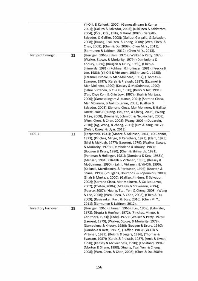
156

Yli-Olli, & Kallunki, 2000); (Gamesalingam & Kumar, 2001); (Gallizo & Salvador, 2003); (Nikkinen & Sahlström, 2004); (Öcal, Oral, Erdis, & Vural, 2007); (Gargallo, Salvador, & Gallizo, 2008); (Gallizo, Gargallo, & Salvador, 2008); (Huang, Tsai, Yen, & Cheng, 2008); (Wen, Chen, & Chen, 2008); (Chen & Du, 2009); (Chen M. Y., 2011); (Sormunen & Laitinen, 2012); (Chen M. Y., 2013).

Net profit margin 33 (Horrigan, 1966); (Elam, 1975); (Walker & Petty, 1978); (Walker, Stowe, & Moriarity, 1979); (Dambolena & Khoury, 1980); (Bougen & Drury, 1980); (Chen & Shimerda, 1981); (Pohlman & Hollinger, 1981); (Frecka & Lee, 1983); (Yli-Olli & Virtanen, 1985); (Lee C. , 1985); (Ezzamel, Brodie, & Mar-Molinero, 1987); (Thomas & Evanson, 1987); (Karels & Prakash, 1987); (Ezzamel & Mar-Molinero, 1990); (Keasey & McGuinness, 1990); (Salmi, Virtanen, & Yli-Olli, 1990); (Berry & Nix, 1991); (Tan, Chye Koh, & Chin Low, 1997); (Shah & Murtaza, 2000); (Gamesalingam & Kumar, 2001); (Serrano Cinca, Mar Molinero, & Gallizo Larraz, 2002); (Gallizo & Salvador, 2003); (Serrano Cinca, Mar Molinero, & Gallizo Larraz, 2005); (Huang, Tsai, Yen, & Cheng, 2008); (Wang & Lee, 2008); (Niemann, Schmidt, & Neukirchen, 2008); (Wen, Chen, & Chen, 2008); (Wang, 2009); (Du Jardin, 2010); (Ng, Wong, & Zhang, 2011); (Kim & Kang, 2012); (Delen, Kuzey, & Uyar, 2013).

ROE 1 33 (Fitzpatrick, 1931); (Moore & Atkinson, 1961); (O'Connor, 1973); (Pinches, Mingo, & Caruthers, 1973); (Elam, 1975); (Bird & McHugh, 1977); (Laurent, 1979); (Walker, Stowe, & Moriarity, 1979); (Dambolena & Khoury, 1980); (Bougen & Drury, 1980); (Chen & Shimerda, 1981); (Pohlman & Hollinger, 1981); (Gombola & Ketz, 1983b); (Mensah, 1984); (Yli-Olli & Virtanen, 1985); (Keasey & McGuinness, 1990); (Salmi, Virtanen, & Yli-Olli, 1990); (Kallunki, Martikainen, & Perttunen, 1996); (Morton & Shane, 1998); (Voulgaris, Doumpos, & Zopounidis, 2000); (Shah & Murtaza, 2000); (Gallizo, Jiménez, & Salvador, 2002); (Serrano Cinca, Mar Molinero, & Gallizo Larraz, 2002); (Costea, 2006); (McLeay & Stevenson, 2006); (Pearce, 2007); (Huang, Tsai, Yen, & Cheng, 2008); (Wang & Lee, 2008); (Wen, Chen, & Chen, 2008); (Chen & Du, 2009); (Ravisankar, Ravi, & Bose, 2010); (Chen M. Y., 2011); (Sormunen & Laitinen, 2012).

Inventory turnover 28 (Horrigan, 1965); (Tamari, 1966); (Lev, 1969); (Edmister, 1972); (Gupta & Huefner, 1972); (Pinches, Mingo, & Caruthers, 1973); (Fadel, 1977); (Walker & Petty, 1978); (Laurent, 1979); (Walker, Stowe, & Moriarity, 1979); (Dambolena & Khoury, 1980); (Bougen & Drury, 1980); (Gombola & Ketz, 1983b); (Taffler, 1983); (Yli-Olli & Virtanen, 1985); (Buijink & Jegers, 1986); (Thomas & Evanson, 1987); (Karels & Prakash, 1987), (Amit & Livnat, 1990); (Keasey & McGuinness, 1990); (Constand, 1994); (Morton & Shane, 1998); (Huang, Tsai, Yen, & Cheng, 2008); (Wen, Chen, & Chen, 2008); (Chen & Du, 2009);

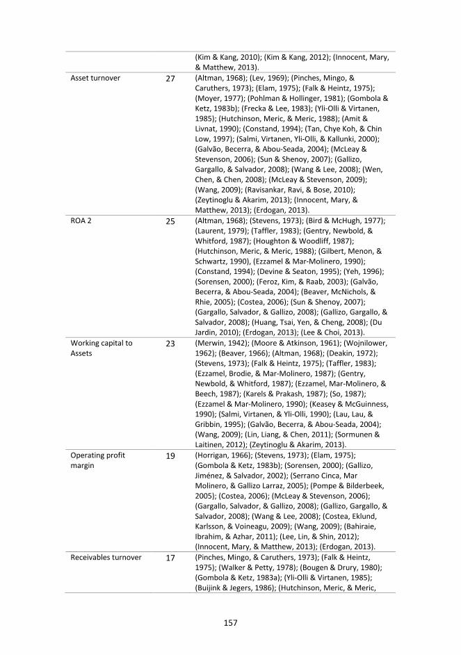
157

(Kim & Kang, 2010); (Kim & Kang, 2012); (Innocent, Mary, & Matthew, 2013).

Asset turnover 27 (Altman, 1968); (Lev, 1969); (Pinches, Mingo, & Caruthers, 1973); (Elam, 1975); (Falk & Heintz, 1975); (Moyer, 1977); (Pohlman & Hollinger, 1981); (Gombola & Ketz, 1983b); (Frecka & Lee, 1983); (Yli-Olli & Virtanen, 1985); (Hutchinson, Meric, & Meric, 1988); (Amit & Livnat, 1990); (Constand, 1994); (Tan, Chye Koh, & Chin Low, 1997); (Salmi, Virtanen, Yli-Olli, & Kallunki, 2000); (Galvão, Becerra, & Abou-Seada, 2004); (McLeay & Stevenson, 2006); (Sun & Shenoy, 2007); (Gallizo, Gargallo, & Salvador, 2008); (Wang & Lee, 2008); (Wen, Chen, & Chen, 2008); (McLeay & Stevenson, 2009); (Wang, 2009); (Ravisankar, Ravi, & Bose, 2010); (Zeytinoglu & Akarim, 2013); (Innocent, Mary, & Matthew, 2013); (Erdogan, 2013).

ROA 2 25 (Altman, 1968); (Stevens, 1973); (Bird & McHugh, 1977); (Laurent, 1979); (Taffler, 1983); (Gentry, Newbold, & Whitford, 1987); (Houghton & Woodliff, 1987); (Hutchinson, Meric, & Meric, 1988); (Gilbert, Menon, & Schwartz, 1990), (Ezzamel & Mar-Molinero, 1990); (Constand, 1994); (Devine & Seaton, 1995); (Yeh, 1996); (Sorensen, 2000); (Feroz, Kim, & Raab, 2003); (Galvão, Becerra, & Abou-Seada, 2004); (Beaver, McNichols, & Rhie, 2005); (Costea, 2006); (Sun & Shenoy, 2007); (Gargallo, Salvador, & Gallizo, 2008); (Gallizo, Gargallo, & Salvador, 2008); (Huang, Tsai, Yen, & Cheng, 2008); (Du Jardin, 2010); (Erdogan, 2013); (Lee & Choi, 2013).

Working capital to Assets

23 (Merwin, 1942); (Moore & Atkinson, 1961); (Wojnilower, 1962); (Beaver, 1966); (Altman, 1968); (Deakin, 1972); (Stevens, 1973); (Falk & Heintz, 1975); (Taffler, 1983); (Ezzamel, Brodie, & Mar-Molinero, 1987); (Gentry, Newbold, & Whitford, 1987); (Ezzamel, Mar-Molinero, & Beech, 1987); (Karels & Prakash, 1987); (So, 1987); (Ezzamel & Mar-Molinero, 1990); (Keasey & McGuinness, 1990); (Salmi, Virtanen, & Yli-Olli, 1990); (Lau, Lau, & Gribbin, 1995); (Galvão, Becerra, & Abou-Seada, 2004); (Wang, 2009); (Lin, Liang, & Chen, 2011); (Sormunen & Laitinen, 2012); (Zeytinoglu & Akarim, 2013).

Operating profit margin

19 (Horrigan, 1966); (Stevens, 1973); (Elam, 1975); (Gombola & Ketz, 1983b); (Sorensen, 2000); (Gallizo, Jiménez, & Salvador, 2002); (Serrano Cinca, Mar Molinero, & Gallizo Larraz, 2005); (Pompe & Bilderbeek, 2005); (Costea, 2006); (McLeay & Stevenson, 2006); (Gargallo, Salvador, & Gallizo, 2008); (Gallizo, Gargallo, & Salvador, 2008); (Wang & Lee, 2008); (Costea, Eklund, Karlsson, & Voineagu, 2009); (Wang, 2009); (Bahiraie, Ibrahim, & Azhar, 2011); (Lee, Lin, & Shin, 2012); (Innocent, Mary, & Matthew, 2013); (Erdogan, 2013).

Receivables turnover 17 (Pinches, Mingo, & Caruthers, 1973); (Falk & Heintz, 1975); (Walker & Petty, 1978); (Bougen & Drury, 1980); (Gombola & Ketz, 1983a); (Yli-Olli & Virtanen, 1985); (Buijink & Jegers, 1986); (Hutchinson, Meric, & Meric,

158

1988); (Shah & Murtaza, 2000), (Costea, 2006); (Huang, Tsai, Yen, & Cheng, 2008); (Wen, Chen, & Chen, 2008); (Costea, Eklund, Karlsson, & Voineagu, 2009); (Wang, 2009); (Du Jardin, 2010); (Innocent, Mary, & Matthew, 2013); (Lee & Choi, 2013).

Working capital turnover

15 (Tamari, 1966); (Horrigan, 1966); (Deakin, 1972); (Edmister, 1972); (O'Connor, 1973); (Laurent, 1979); (Walker, Stowe, & Moriarity, 1979); (Dambolena & Khoury, 1980); (Ezzamel & Mar-Molinero, 1990); (Lau, Lau, & Gribbin, 1995); (Morton & Shane, 1998); (Öcal, Oral, Erdis, & Vural, 2007); (De, Bandyopadhyay, & Chakraborty, 2011); (Sormunen & Laitinen, 2012); (Lee & Choi, 2013).

Current assets turnover

14 (Deakin, 1972); (Libby, 1975); (Frecka & Hopwood, 1983); (McDonald & Morris, 1984); (Casey & Bartczak, 1985); (Ezzamel, Mar-Molinero, & Beech, 1987); (Watson, 1990); (Berry & Nix, 1991); (Devine & Seaton, 1995); (Lau, Lau, & Gribbin, 1995); (Sun & Shenoy, 2007); (Wang, 2009); (Ng, Wong, & Zhang, 2011); (Yap, Mohamad, & Chong, 2013).

Equity to Assets 12 (Walker, Stowe, & Moriarity, 1979); (Hutchinson, Meric, & Meric, 1988); (Yeh, 1996); (Zanakis & Zopounidis, 1997); (Voulgaris, Doumpos, & Zopounidis, 2000); (Shah & Murtaza, 2000); (Serrano Cinca, Mar Molinero, & Gallizo Larraz, 2005); (Costea, 2006); (Huang, Tsai, Yen, & Cheng, 2008); (Min & Lee, 2008); (Du Jardin, 2010); (Zeytinoglu & Akarim, 2013).

Current assets to Total assets

12 (Deakin, 1972); (Chen & Shimerda, 1981); (Casey & Bartczak, 1985); (So, 1987); (Hutchinson, Meric, & Meric, 1988); (Lau, Lau, & Gribbin, 1995); (Sun & Shenoy, 2007); (Chen & Du, 2009); (Ravisankar, Ravi, & Bose, 2010); (Bahiraie, Ibrahim, & Azhar, 2011); (Chen M. Y., 2011); (Chen M. Y., 2013).

Times interest earned ratio

12 (Yli-Olli & Virtanen, 1985); (Shah & Murtaza, 2000); (Serrano Cinca, Mar Molinero, & Gallizo Larraz, 2002); (Serrano Cinca, Mar Molinero, & Gallizo Larraz, 2005); (Costea, 2006); (Pearce, 2007); (Huang, Tsai, Yen, & Cheng, 2008); (Min & Lee, 2008); (Niemann, Schmidt, & Neukirchen, 2008); (Costea, Eklund, Karlsson, & Voineagu, 2009); (Vuran, 2009); (Ng, Wong, & Zhang, 2011).

Operating cash flow to Total liabilities

12 (Lee C. , 1985); (Gentry, Newbold, & Whitford, 1987); (Houghton & Woodliff, 1987); (So, 1987); (Berry & Nix, 1991); (Lau, Lau, & Gribbin, 1995); (Zanakis & Zopounidis, 1997); (Sun & Shenoy, 2007); (Chen & Du, 2009); (Chen M. Y., 2011); (Sormunen & Laitinen, 2012); (Lee & Choi, 2013).

Quick assets to Total assets

10 (Deakin, 1972); (Pohlman & Hollinger, 1981); (Taffler, 1983); (Frecka & Hopwood, 1983); (Ezzamel, Brodie, & Mar-Molinero, 1987); (Ezzamel & Mar-Molinero, 1990); (Lau, Lau, & Gribbin, 1995); (Pompe & Bilderbeek, 2005); (Du Jardin, 2010); (Ng, Wong, & Zhang, 2011).

Cash ratio 10 (Deakin, 1972); (Elam, 1975); (Tan, Chye Koh, & Chin Low, 1997); (Gamesalingam & Kumar, 2001); (Peel, Peel, &

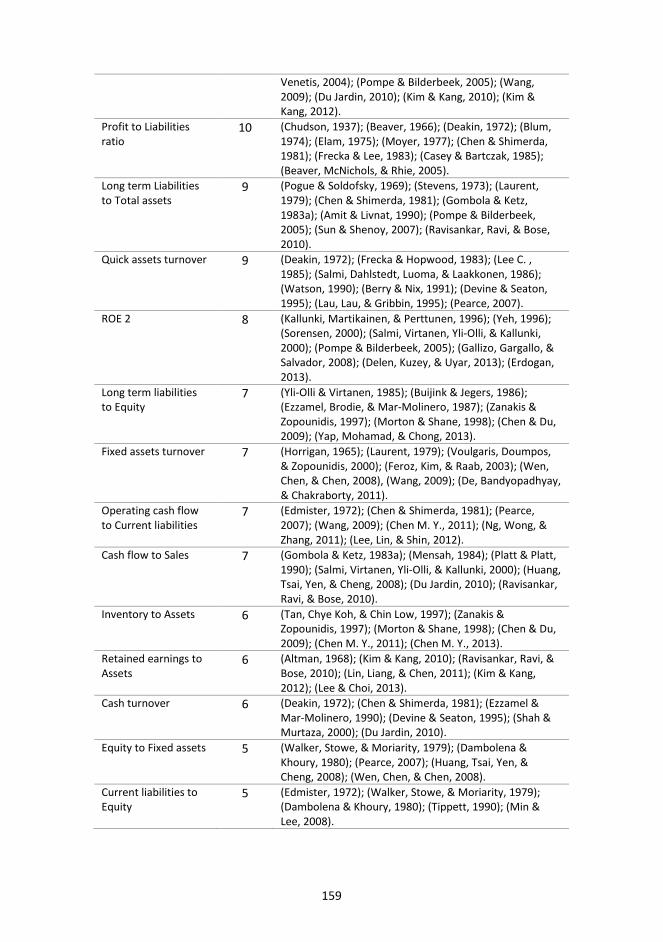
159

Venetis, 2004); (Pompe & Bilderbeek, 2005); (Wang, 2009); (Du Jardin, 2010); (Kim & Kang, 2010); (Kim & Kang, 2012).

Profit to Liabilities ratio

10 (Chudson, 1937); (Beaver, 1966); (Deakin, 1972); (Blum, 1974); (Elam, 1975); (Moyer, 1977); (Chen & Shimerda, 1981); (Frecka & Lee, 1983); (Casey & Bartczak, 1985); (Beaver, McNichols, & Rhie, 2005).

Long term Liabilities to Total assets

9 (Pogue & Soldofsky, 1969); (Stevens, 1973); (Laurent, 1979); (Chen & Shimerda, 1981); (Gombola & Ketz, 1983a); (Amit & Livnat, 1990); (Pompe & Bilderbeek, 2005); (Sun & Shenoy, 2007); (Ravisankar, Ravi, & Bose, 2010).

Quick assets turnover 9 (Deakin, 1972); (Frecka & Hopwood, 1983); (Lee C. , 1985); (Salmi, Dahlstedt, Luoma, & Laakkonen, 1986); (Watson, 1990); (Berry & Nix, 1991); (Devine & Seaton, 1995); (Lau, Lau, & Gribbin, 1995); (Pearce, 2007).

ROE 2 8 (Kallunki, Martikainen, & Perttunen, 1996); (Yeh, 1996); (Sorensen, 2000); (Salmi, Virtanen, Yli-Olli, & Kallunki, 2000); (Pompe & Bilderbeek, 2005); (Gallizo, Gargallo, & Salvador, 2008); (Delen, Kuzey, & Uyar, 2013); (Erdogan, 2013).

Long term liabilities to Equity

7 (Yli-Olli & Virtanen, 1985); (Buijink & Jegers, 1986); (Ezzamel, Brodie, & Mar-Molinero, 1987); (Zanakis & Zopounidis, 1997); (Morton & Shane, 1998); (Chen & Du, 2009); (Yap, Mohamad, & Chong, 2013).

Fixed assets turnover 7 (Horrigan, 1965); (Laurent, 1979); (Voulgaris, Doumpos, & Zopounidis, 2000); (Feroz, Kim, & Raab, 2003); (Wen, Chen, & Chen, 2008), (Wang, 2009); (De, Bandyopadhyay, & Chakraborty, 2011).

Operating cash flow to Current liabilities

7 (Edmister, 1972); (Chen & Shimerda, 1981); (Pearce, 2007); (Wang, 2009); (Chen M. Y., 2011); (Ng, Wong, & Zhang, 2011); (Lee, Lin, & Shin, 2012).

Cash flow to Sales 7 (Gombola & Ketz, 1983a); (Mensah, 1984); (Platt & Platt, 1990); (Salmi, Virtanen, Yli-Olli, & Kallunki, 2000); (Huang, Tsai, Yen, & Cheng, 2008); (Du Jardin, 2010); (Ravisankar, Ravi, & Bose, 2010).

Inventory to Assets 6 (Tan, Chye Koh, & Chin Low, 1997); (Zanakis & Zopounidis, 1997); (Morton & Shane, 1998); (Chen & Du, 2009); (Chen M. Y., 2011); (Chen M. Y., 2013).

Retained earnings to Assets

6 (Altman, 1968); (Kim & Kang, 2010); (Ravisankar, Ravi, & Bose, 2010); (Lin, Liang, & Chen, 2011); (Kim & Kang, 2012); (Lee & Choi, 2013).

Cash turnover 6 (Deakin, 1972); (Chen & Shimerda, 1981); (Ezzamel & Mar-Molinero, 1990); (Devine & Seaton, 1995); (Shah & Murtaza, 2000); (Du Jardin, 2010).

Equity to Fixed assets 5 (Walker, Stowe, & Moriarity, 1979); (Dambolena & Khoury, 1980); (Pearce, 2007); (Huang, Tsai, Yen, & Cheng, 2008); (Wen, Chen, & Chen, 2008).

Current liabilities to Equity

5 (Edmister, 1972); (Walker, Stowe, & Moriarity, 1979); (Dambolena & Khoury, 1980); (Tippett, 1990); (Min & Lee, 2008).

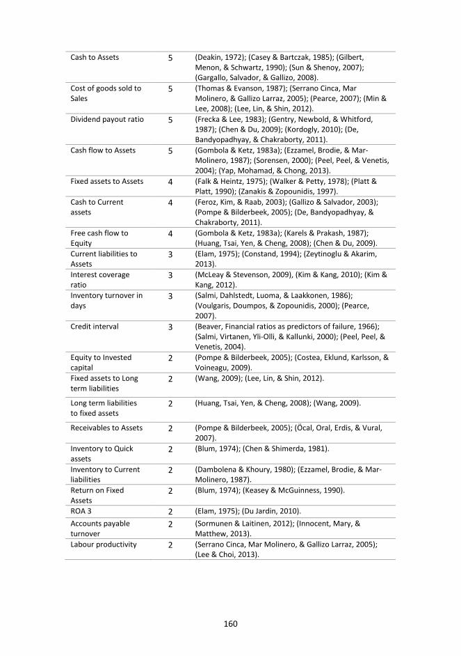
160

Cash to Assets 5 (Deakin, 1972); (Casey & Bartczak, 1985); (Gilbert, Menon, & Schwartz, 1990); (Sun & Shenoy, 2007); (Gargallo, Salvador, & Gallizo, 2008).

Cost of goods sold to Sales

5 (Thomas & Evanson, 1987); (Serrano Cinca, Mar Molinero, & Gallizo Larraz, 2005); (Pearce, 2007); (Min & Lee, 2008); (Lee, Lin, & Shin, 2012).

Dividend payout ratio 5 (Frecka & Lee, 1983); (Gentry, Newbold, & Whitford, 1987); (Chen & Du, 2009); (Kordogly, 2010); (De, Bandyopadhyay, & Chakraborty, 2011).

Cash flow to Assets 5 (Gombola & Ketz, 1983a); (Ezzamel, Brodie, & Mar-Molinero, 1987); (Sorensen, 2000); (Peel, Peel, & Venetis, 2004); (Yap, Mohamad, & Chong, 2013).

Fixed assets to Assets 4 (Falk & Heintz, 1975); (Walker & Petty, 1978); (Platt & Platt, 1990); (Zanakis & Zopounidis, 1997).

Cash to Current assets

4 (Feroz, Kim, & Raab, 2003); (Gallizo & Salvador, 2003); (Pompe & Bilderbeek, 2005); (De, Bandyopadhyay, & Chakraborty, 2011).

Free cash flow to Equity

4 (Gombola & Ketz, 1983a); (Karels & Prakash, 1987); (Huang, Tsai, Yen, & Cheng, 2008); (Chen & Du, 2009).

Current liabilities to Assets

3 (Elam, 1975); (Constand, 1994); (Zeytinoglu & Akarim, 2013).

Interest coverage ratio

3 (McLeay & Stevenson, 2009), (Kim & Kang, 2010); (Kim & Kang, 2012).

Inventory turnover in days

3 (Salmi, Dahlstedt, Luoma, & Laakkonen, 1986); (Voulgaris, Doumpos, & Zopounidis, 2000); (Pearce, 2007).

Credit interval 3 (Beaver, Financial ratios as predictors of failure, 1966); (Salmi, Virtanen, Yli-Olli, & Kallunki, 2000); (Peel, Peel, & Venetis, 2004).

Equity to Invested capital

2 (Pompe & Bilderbeek, 2005); (Costea, Eklund, Karlsson, & Voineagu, 2009).

Fixed assets to Long term liabilities

2 (Wang, 2009); (Lee, Lin, & Shin, 2012).

Long term liabilities to fixed assets

2 (Huang, Tsai, Yen, & Cheng, 2008); (Wang, 2009).

Receivables to Assets 2 (Pompe & Bilderbeek, 2005); (Öcal, Oral, Erdis, & Vural, 2007).

Inventory to Quick assets

2 (Blum, 1974); (Chen & Shimerda, 1981).

Inventory to Current liabilities

2 (Dambolena & Khoury, 1980); (Ezzamel, Brodie, & Mar-Molinero, 1987).

Return on Fixed Assets

2 (Blum, 1974); (Keasey & McGuinness, 1990).

ROA 3 2 (Elam, 1975); (Du Jardin, 2010). Accounts payable turnover

2 (Sormunen & Laitinen, 2012); (Innocent, Mary, & Matthew, 2013).

Labour productivity 2 (Serrano Cinca, Mar Molinero, & Gallizo Larraz, 2005); (Lee & Choi, 2013).

161

Appendix 3. Interpretation of cash-based ratios used in company’s overall efficiency matrix A. Free cash flow to Net operating cash flow

Net operating cash flow

(R)

Net investing

cash flow

Free cash

flow (F) F/R Explanation

>0

<0

≤0 ≤0

Net operating cash flow is not sufficient to cover investing cash outflow. Cash earned in previous periods or financing cash inflow have to be used to cover investing cash outflow. Typical for growing companies.

>0

0<x<1

Net operating cash flow is sufficient to cover investing cash outflow. Positive free cash flow could be used to reduce capital employed or improve the cash position. Typical for developed companies.

≥0

≥1

Net operating cash flow and net investing cash flow both positive. The company is increasing liquidity either to improve cash position (for the future investments) or needs to reduce capital employed (pay back loans). Typical for companies enforcing restructurings or having a high proportion of loans from capital employed.

<0

≥0 ≤0

Negative net operating cash flow is fully offset by investing cash inflow. The company is either selling non-core assets to improve liquidity or needs to reduce capital employed (pay back loans). Typical for companies enforcing restructurings or having a high proportion of loans from capital employed.

<0 0<x<1

Negative net operating cash flow is partially offset by investing cash inflow. Cash earned in previous periods or financing cash inflow (capital injection from owners) used to cover negative free cash flow. Typical for companies with a business turnaround.

162

≤0 ≥1

Net operating cash flow and net investing cash flow both negative. Increase in capital employed is used to cover negative free cash flow. Typical for companies in the starting phase.

Source: (by author).

B. Free cash flow to Profit (EBIT)

Free cash

flow (F) Profit

(P) F/P Explanation

≥0

>0

0≤x≤1 Some of the profit earned is used to finance new investments. Typical for developed companies.

>0

>1

Positive free cash flow exceeds profit. This could be explained by payments received (sales were recorded in the previous period) and/or positive net investing cash flow (e.g. sales of non-core assets). Typical for companies either offering long payment deadlines for customers or restructuring the business.

<0

<0

Free cash flow positive, despite loss. This could be explained by payments received (sales were recorded in the previous period) and/or positive net investing cash flow (e.g. sales of non-core assets). Typical for companies either offering long payment terms for the customers or restructuring the business.

<0

>1

Negative value of free cash flow exceeds negative value of loss. This could be explained by continuous investment cash outflow financed by capital payments. Typical for companies in the starting phase.

0<x≤1

Negative free cash flow lower than or equal to loss. This could be explained by postponed payments to suppliers and/or positive net investing cash flow (e.g. sales of non-core assets). Typical for companies either receiving long payment deadlines from suppliers or restructuring the business.

>0 <0

Despite profitability free cash flow is negative. This could be explained by continuous investment cash outflow financed by capital payments. Typical for growing companies.

Source: (by author).

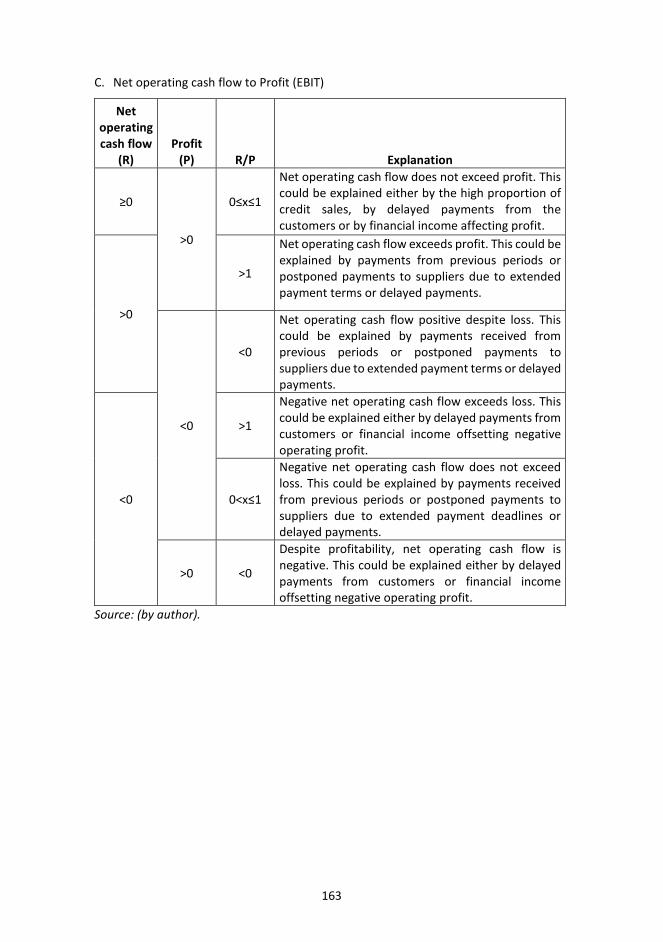
163

C. Net operating cash flow to Profit (EBIT)

Net operating cash flow

(R) Profit

(P) R/P Explanation

≥0

>0

0≤x≤1

Net operating cash flow does not exceed profit. This could be explained either by the high proportion of credit sales, by delayed payments from the customers or by financial income affecting profit.

>0

>1

Net operating cash flow exceeds profit. This could be explained by payments from previous periods or postponed payments to suppliers due to extended payment terms or delayed payments.

<0

<0

Net operating cash flow positive despite loss. This could be explained by payments received from previous periods or postponed payments to suppliers due to extended payment terms or delayed payments.

<0

>1

Negative net operating cash flow exceeds loss. This could be explained either by delayed payments from customers or financial income offsetting negative operating profit.

0<x≤1

Negative net operating cash flow does not exceed loss. This could be explained by payments received from previous periods or postponed payments to suppliers due to extended payment deadlines or delayed payments.

>0 <0

Despite profitability, net operating cash flow is negative. This could be explained either by delayed payments from customers or financial income offsetting negative operating profit.

Source: (by author).

164

Appendix 4. Relationships between the elements of a reverse efficiency field This appendix supplements subchapter 2.2.1, where relationships between the elements of the efficiency field were introduced. Since a reverse efficiency field is the mirror image of an efficiency field, analogous relationships may also be created in relation to relationships between reverse efficiency field elements.

1) If we are interested in the relationship between the element 𝑥𝑥𝑝𝑝𝑖𝑖 (i, j = 1, 2, …, n; i < j)of the reverse efficiency field and the element 𝑥𝑥𝑝𝑝,𝑖𝑖–𝑘𝑘 (k = 1, 2, …) to the left of it in the same row, the element 𝑥𝑥𝑝𝑝,𝑖𝑖–𝑘𝑘 needs to be multiplied by the main elements of the reverse efficiency field to the right of the indicator 𝑥𝑥𝑝𝑝,𝑖𝑖–𝑘𝑘. To prove the claim, we convert the formula (2.11) as follows:

𝑥𝑥𝑝𝑝𝑖𝑖 = 𝑥𝑥𝑝𝑝,𝑝𝑝+1 × 𝑥𝑥𝑝𝑝+1,𝑝𝑝+2 … 𝑥𝑥𝑖𝑖–𝑘𝑘–1,𝑖𝑖–𝑘𝑘 × 𝑥𝑥𝑖𝑖–𝑘𝑘,𝑖𝑖–𝑘𝑘+1 … 𝑥𝑥𝑖𝑖–2,𝑖𝑖–1 × 𝑥𝑥𝑖𝑖–1,𝑖𝑖 (A4.1)

and the element to be associated may be expressed analogously:

𝑥𝑥𝑝𝑝,𝑖𝑖–𝑘𝑘 = 𝑥𝑥𝑝𝑝,𝑝𝑝+1 × 𝑥𝑥𝑝𝑝+1,𝑝𝑝+2 … 𝑥𝑥𝑖𝑖–𝑘𝑘–1,𝑖𝑖–𝑘𝑘 (A4.2)

By replacing the formula (A4.1) into the formula (A4.2), we obtain the expression:

𝑥𝑥𝑝𝑝𝑖𝑖 = 𝑥𝑥𝑝𝑝,𝑖𝑖–𝑘𝑘 × 𝑥𝑥𝑖𝑖–𝑘𝑘,𝑖𝑖–𝑘𝑘+1 … 𝑥𝑥𝑖𝑖–2,𝑖𝑖–1 × 𝑥𝑥𝑖𝑖–1,𝑖𝑖 (A4.3)

Example. Let it be necessary, based on the company’s overall efficiency matrix (Table 2.2), to ascertain the relationship between the elements 𝑥𝑥15 (Operating expenses to Free cash flow) and 𝑥𝑥13 (EBIT to Free cash flow). In this case, i = 1; j = 5; k = 5 - 3 = 2. By expressing both elements through the main elements, we obtain

𝑥𝑥15 = 𝑥𝑥12 × 𝑥𝑥23 × 𝑥𝑥34 × 𝑥𝑥45 and 𝑥𝑥13 = 𝑥𝑥12 × 𝑥𝑥23

and consequently

𝑥𝑥15 = 𝑥𝑥13 × 𝑥𝑥34 × 𝑥𝑥45 = 𝑥𝑥13 × 𝑥𝑥35.

This means that Operating expenses to Free cash flow = = EBIT to Free cash flow × Sales to Profit × Operating expenses to Sales = = EBIT to Free cash flow × Operating expenses to Profit.

In addition, there is the option of interlinking the main elements of an efficiency field and a reverse efficiency field, using for this the reverse values of the main elements of the relevant fields and replacing the multiplication by division. Hence,

𝑥𝑥𝑝𝑝𝑖𝑖 =𝑥𝑥𝑖𝑖,𝑖𝑖–𝑘𝑘

𝑥𝑥𝑖𝑖–𝑘𝑘+1,𝑖𝑖–𝑘𝑘… 𝑥𝑥𝑖𝑖–1,𝑖𝑖–2×𝑥𝑥𝑖𝑖,𝑖𝑖–1(A4.4)

Example. The relationship between the elements 𝑥𝑥15 (Operating expenses to Free cash flow) and 𝑥𝑥13 (EBIT to Free cash flow) may also be expressed in the form:

𝑥𝑥15 = 𝑥𝑥13𝑥𝑥43×𝑥𝑥54

= 𝑥𝑥13𝑥𝑥53

.

2) If we are interested in the relationship between the element 𝑥𝑥𝑝𝑝𝑖𝑖 (i, j = 1, 2, …, n; i < j)of the reverse efficiency field and the element 𝑥𝑥𝑝𝑝–𝑇𝑇,𝑖𝑖 (l = 1, 2, …) above it in the same row, the element 𝑥𝑥𝑝𝑝–𝑇𝑇,𝑖𝑖 needs to be divided by the main elements of the reverse efficiency field, up of the element 𝑥𝑥𝑝𝑝,𝑖𝑖 or needs to be multiplied by the reverse values of these

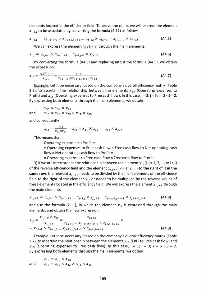
165

elements located in the efficiency field. To prove the claim, we will express the element 𝑥𝑥𝑝𝑝–𝑇𝑇,𝑖𝑖 to be associated by converting the formula (2.11) as follows:

𝑥𝑥𝑝𝑝–𝑇𝑇,𝑖𝑖 = 𝑥𝑥𝑝𝑝–𝑇𝑇,𝑝𝑝–𝑇𝑇+1 × 𝑥𝑥𝑝𝑝–𝑇𝑇+1,𝑝𝑝–𝑇𝑇+2 … 𝑥𝑥𝑝𝑝–1,𝑝𝑝 × 𝑥𝑥𝑝𝑝,𝑝𝑝+1 … 𝑥𝑥𝑖𝑖–2,𝑖𝑖–1 × 𝑥𝑥𝑖𝑖–1,𝑖𝑖 (A4.5)

We can express the element 𝑥𝑥𝑝𝑝,𝑖𝑖 (i < j) through the main elements:

𝑥𝑥𝑝𝑝,𝑖𝑖 = 𝑥𝑥𝑝𝑝,𝑝𝑝+1 × 𝑥𝑥𝑝𝑝+1,𝑝𝑝+2 … 𝑥𝑥𝑖𝑖–2,𝑖𝑖–1 × 𝑥𝑥𝑖𝑖–1,𝑖𝑖 (A4.6)

By converting the formula (A4.6) and replacing into it the formula (A4.5), we obtain the expression:

𝑥𝑥𝑝𝑝𝑖𝑖 =𝑥𝑥𝑖𝑖,𝑖𝑖×𝑥𝑥𝑖𝑖,𝑖𝑖–𝑙𝑙

𝑥𝑥𝑖𝑖,𝑖𝑖–𝑙𝑙=

𝑥𝑥𝑖𝑖,𝑖𝑖–𝑙𝑙

𝑥𝑥𝑖𝑖–𝑙𝑙,𝑖𝑖–𝑙𝑙+1×𝑥𝑥𝑖𝑖–𝑙𝑙+1,𝑖𝑖–𝑙𝑙+2… 𝑥𝑥𝑖𝑖–1,𝑖𝑖(A4.7)

Example. Let it be necessary, based on the company’s overall efficiency matrix (Table 2.2), to ascertain the relationship between the elements 𝑥𝑥35 (Operating expenses to Profit) and 𝑥𝑥15 (Operating expenses to Free cash flow). In this case, i = 3; j = 5; l = 3 - 1 = 2. By expressing both elements through the main elements, we obtain

𝑥𝑥35 = 𝑥𝑥34 × 𝑥𝑥45 and 𝑥𝑥15 = 𝑥𝑥12 × 𝑥𝑥23 × 𝑥𝑥34 × 𝑥𝑥45

and consequently

𝑥𝑥35 = 𝑥𝑥15𝑥𝑥12×𝑥𝑥23

= 𝑥𝑥15 × 𝑥𝑥21 × 𝑥𝑥32 = 𝑥𝑥15 × 𝑥𝑥31.

This means that Operating expenses to Profit = = Operating expenses to Free cash flow × Free cash flow to Net operating cash flow × Net operating cash flow to Profit = = Operating expenses to Free cash flow × Free cash flow to Profit.

3) If we are interested in the relationship between the element 𝑥𝑥𝑝𝑝𝑖𝑖 (i, j = 1, 2, …, n; i < j)of the reverse efficiency field and the element 𝑥𝑥𝑝𝑝,𝑖𝑖+𝑘𝑘 (k = 1, 2, …) to the right of it in the same row, the relevant 𝑥𝑥𝑝𝑝,𝑖𝑖+𝑘𝑘 needs to be divided by the main elements of the efficiency field to the right of the element 𝑥𝑥𝑝𝑝𝑖𝑖 or needs to be multiplied by the reverse values of these elements located in the efficiency field. We will express the element 𝑥𝑥𝑝𝑝,𝑖𝑖+𝑘𝑘 through the main elements

𝑥𝑥𝑝𝑝,𝑖𝑖+𝑘𝑘 = 𝑥𝑥𝑝𝑝,𝑝𝑝+1 × 𝑥𝑥𝑝𝑝+1,𝑝𝑝+2 … 𝑥𝑥𝑖𝑖–1,𝑖𝑖 × 𝑥𝑥𝑖𝑖,𝑖𝑖+1 … 𝑥𝑥𝑖𝑖+𝑘𝑘–2,𝑖𝑖+𝑘𝑘–1 × 𝑥𝑥𝑖𝑖+𝑘𝑘–1,𝑖𝑖+𝑘𝑘 (A4.8)

and use the formula (2.11), in which the element 𝑥𝑥𝑝𝑝𝑖𝑖 is expressed through the main elements, and obtain the new expression:

𝑥𝑥𝑝𝑝𝑖𝑖 =𝑥𝑥𝑝𝑝,𝑖𝑖+𝑘𝑘 × 𝑥𝑥𝑝𝑝𝑖𝑖𝑥𝑥𝑝𝑝,𝑖𝑖+𝑘𝑘

=𝑥𝑥𝑝𝑝,𝑖𝑖+𝑘𝑘

𝑥𝑥𝑖𝑖,𝑖𝑖+1 … 𝑥𝑥𝑖𝑖+𝑘𝑘–2,𝑖𝑖+𝑘𝑘–1 × 𝑥𝑥𝑖𝑖+𝑘𝑘–1,𝑖𝑖+𝑘𝑘=

= 𝑥𝑥𝑝𝑝,𝑖𝑖+𝑘𝑘 × 𝑥𝑥𝑖𝑖+1,𝑖𝑖 … 𝑥𝑥𝑖𝑖+𝑘𝑘–1,𝑖𝑖+𝑘𝑘–2 × 𝑥𝑥𝑖𝑖+𝑘𝑘,𝑖𝑖+𝑘𝑘–1 (A4.9)

Example. Let it be necessary, based on the company’s overall efficiency matrix (Table 2.2), to ascertain the relationship between the elements 𝑥𝑥13 (EBIT to Free cash flow) and 𝑥𝑥15 (Operating expenses to Free cash flow). In this case, i = 1; j = 3; k = 5 - 3 = 2. By expressing both elements through the main elements, we obtain

𝑥𝑥13 = 𝑥𝑥12 × 𝑥𝑥23 and 𝑥𝑥15 = 𝑥𝑥12 × 𝑥𝑥23 × 𝑥𝑥34 × 𝑥𝑥45

166

and consequently

𝑥𝑥13 =𝑥𝑥15

𝑥𝑥34 × 𝑥𝑥45= 𝑥𝑥15 × 𝑥𝑥43 × 𝑥𝑥54 = 𝑥𝑥15 × 𝑥𝑥53

This means that EBIT to Free cash flow = = Operating expenses to Free cash flow × EBIT to Sales × Sales to Operating expenses = Operating expenses to Free cash flow × EBIT to Operating expenses.

4) If we are interested in the relationship between the element 𝑥𝑥𝑝𝑝𝑖𝑖 (i, j = 1, 2, …, n; i < j)of the reverse efficiency field and the element 𝑥𝑥𝑝𝑝+𝑇𝑇,𝑖𝑖 (l = 1, 2, …) below it in the same column, the element 𝑥𝑥𝑝𝑝+𝑇𝑇,𝑖𝑖 needs to be multiplied by the main elements of the reverse efficiency field above the element 𝑥𝑥𝑝𝑝+𝑇𝑇,𝑖𝑖. To prove the claim, we will express the element 𝑥𝑥𝑝𝑝+𝑇𝑇,𝑖𝑖 to be associated by converting the formula (2.11) as follows:

𝑥𝑥𝑝𝑝+𝑇𝑇,𝑖𝑖 = 𝑥𝑥𝑝𝑝+𝑇𝑇,𝑝𝑝+𝑇𝑇+1 × 𝑥𝑥𝑝𝑝+𝑇𝑇+1,𝑝𝑝+𝑇𝑇+2 … 𝑥𝑥𝑖𝑖–2,𝑖𝑖–1 × 𝑥𝑥𝑖𝑖–1,𝑖𝑖 (A4.10)

We can express the element 𝑥𝑥𝑝𝑝𝑖𝑖 (i < j) through the main elements:

𝑥𝑥𝑝𝑝,𝑖𝑖 = 𝑥𝑥𝑝𝑝,𝑝𝑝+1 × 𝑥𝑥𝑝𝑝+1,𝑝𝑝+2 … 𝑥𝑥𝑝𝑝+𝑇𝑇–1,𝑝𝑝+𝑇𝑇 𝑥𝑥𝑝𝑝+𝑇𝑇,𝑝𝑝+𝑇𝑇+1 … 𝑥𝑥𝑖𝑖–2,𝑖𝑖–1 × 𝑥𝑥𝑖𝑖–1,𝑖𝑖 (A4.11)

By converting the formula (A4.11) and replacing into it the formula (A4.10), we obtain the expression:

𝑥𝑥𝑝𝑝𝑖𝑖 = 𝑥𝑥𝑖𝑖+𝑙𝑙,𝑖𝑖×𝑥𝑥𝑖𝑖𝑖𝑖𝑥𝑥𝑖𝑖+𝑙𝑙,𝑖𝑖

= 𝑥𝑥𝑝𝑝+𝑇𝑇,𝑖𝑖 × 𝑥𝑥𝑝𝑝,𝑝𝑝+1 × 𝑥𝑥𝑝𝑝+1,𝑝𝑝+2 … 𝑥𝑥𝑝𝑝+𝑇𝑇–1,𝑝𝑝+𝑇𝑇 (A4.12)

Example. Let it be necessary, based on the company’s overall efficiency matrix (Table 2.2), to ascertain the relationship between the elements 𝑥𝑥15 (Operating expenses to Free cash flow) and 𝑥𝑥35 (Operating expenses to Profit). In this case, i = 1; j = 5; l = 5 - 3 = 2. By expressing both elements through the main elements, we obtain

𝑥𝑥15 = 𝑥𝑥12 × 𝑥𝑥23 × 𝑥𝑥34 × 𝑥𝑥45 and 𝑥𝑥35 = 𝑥𝑥34 × 𝑥𝑥45

and consequently

𝑥𝑥15 = 𝑥𝑥35 × 𝑥𝑥12 × 𝑥𝑥23 = 𝑥𝑥35 × 𝑥𝑥13.

This means that Operating expenses to Free cash flow = Operating expenses to Profit × Net operating cash flow to Free cash flow × EBIT to Net operating cash flow = Op. expenses to Profit × EBIT to Free cash flow.

5) If we are interested in the relationship between the element 𝑥𝑥𝑝𝑝𝑖𝑖 (i, j = 1, 2, …, n; i < j)of the reverse efficiency field and the element 𝑥𝑥𝑝𝑝–𝑇𝑇,𝑖𝑖–𝑘𝑘 (k = 1, 2, …; l = 1, 2, …) above it to the left, the relevant element 𝑥𝑥𝑝𝑝–𝑇𝑇,𝑖𝑖–𝑘𝑘 needs to be multiplied by the main elements of the reverse efficiency field to the right of it and needs to be divided by the main elements of the reverse efficiency field up to the element 𝑥𝑥𝑝𝑝𝑖𝑖 (or multiplied by the relevant main elements of the efficiency field). To prove the claim, we express the element 𝑥𝑥𝑝𝑝𝑖𝑖 using the formula (A4.1):

𝑥𝑥𝑝𝑝𝑖𝑖 = 𝑥𝑥𝑝𝑝,𝑝𝑝+1 × 𝑥𝑥𝑝𝑝+1,𝑝𝑝+2 … 𝑥𝑥𝑖𝑖–𝑘𝑘–1,𝑖𝑖–𝑘𝑘 × 𝑥𝑥𝑖𝑖–𝑘𝑘,𝑖𝑖–𝑘𝑘+1 … 𝑥𝑥𝑖𝑖–2,𝑖𝑖–1 × 𝑥𝑥𝑖𝑖–1,𝑖𝑖

and present the element 𝑥𝑥𝑝𝑝–𝑇𝑇,𝑖𝑖–𝑘𝑘 to be associated in the form:

𝑥𝑥𝑝𝑝–𝑇𝑇,𝑖𝑖–𝑘𝑘 = 𝑥𝑥𝑝𝑝–𝑇𝑇,𝑝𝑝–𝑇𝑇+1 × 𝑥𝑥𝑝𝑝–𝑇𝑇+1,𝑝𝑝–𝑇𝑇+2 … 𝑥𝑥𝑝𝑝–1,𝑝𝑝 × 𝑥𝑥𝑝𝑝,𝑝𝑝+1 … 𝑥𝑥𝑖𝑖–𝑘𝑘–1,𝑝𝑝–𝑘𝑘 (A4.13)

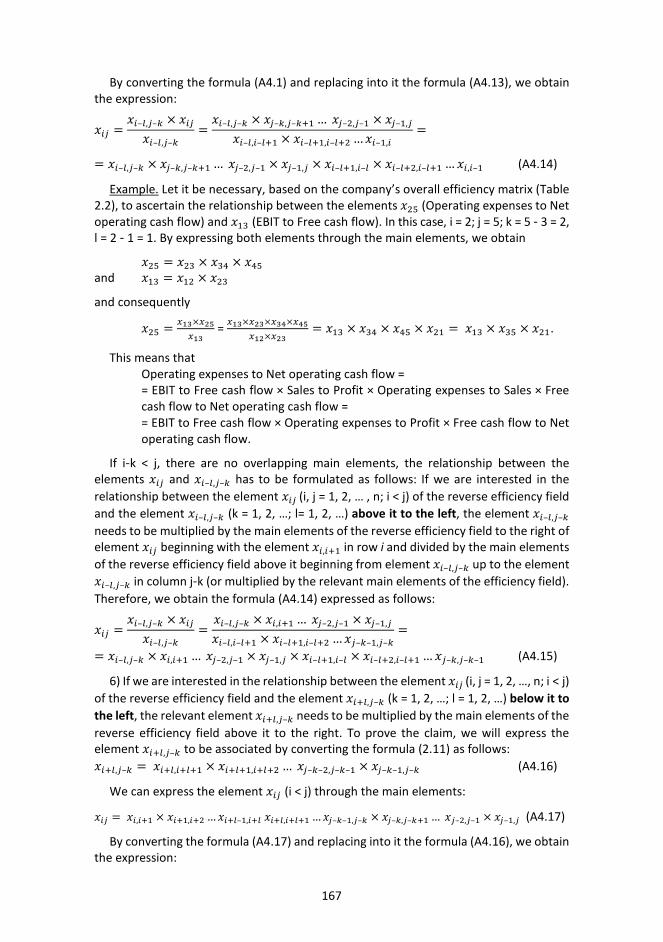
167

By converting the formula (A4.1) and replacing into it the formula (A4.13), we obtain the expression:

𝑥𝑥𝑝𝑝𝑖𝑖 =𝑥𝑥𝑝𝑝–𝑇𝑇,𝑖𝑖–𝑘𝑘 × 𝑥𝑥𝑝𝑝𝑖𝑖𝑥𝑥𝑝𝑝–𝑇𝑇,𝑖𝑖–𝑘𝑘

=𝑥𝑥𝑝𝑝–𝑇𝑇,𝑖𝑖–𝑘𝑘 × 𝑥𝑥𝑖𝑖–𝑘𝑘,𝑖𝑖–𝑘𝑘+1 … 𝑥𝑥𝑖𝑖–2,𝑖𝑖–1 × 𝑥𝑥𝑖𝑖–1,𝑖𝑖

𝑥𝑥𝑝𝑝–𝑇𝑇,𝑝𝑝–𝑇𝑇+1 × 𝑥𝑥𝑝𝑝–𝑇𝑇+1,𝑝𝑝–𝑇𝑇+2 … 𝑥𝑥𝑝𝑝–1,𝑝𝑝=

= 𝑥𝑥𝑝𝑝–𝑇𝑇,𝑖𝑖–𝑘𝑘 × 𝑥𝑥𝑖𝑖–𝑘𝑘,𝑖𝑖–𝑘𝑘+1 … 𝑥𝑥𝑖𝑖–2,𝑖𝑖–1 × 𝑥𝑥𝑖𝑖–1,𝑖𝑖 × 𝑥𝑥𝑝𝑝–𝑇𝑇+1,𝑝𝑝–𝑇𝑇 × 𝑥𝑥𝑝𝑝–𝑇𝑇+2,𝑝𝑝–𝑇𝑇+1 … 𝑥𝑥𝑝𝑝,𝑝𝑝–1 (A4.14)

Example. Let it be necessary, based on the company’s overall efficiency matrix (Table 2.2), to ascertain the relationship between the elements 𝑥𝑥25 (Operating expenses to Net operating cash flow) and 𝑥𝑥13 (EBIT to Free cash flow). In this case, i = 2; j = 5; k = 5 - 3 = 2, l = 2 - 1 = 1. By expressing both elements through the main elements, we obtain

𝑥𝑥25 = 𝑥𝑥23 × 𝑥𝑥34 × 𝑥𝑥45 and 𝑥𝑥13 = 𝑥𝑥12 × 𝑥𝑥23

and consequently

𝑥𝑥25 = 𝑥𝑥13×𝑥𝑥25𝑥𝑥13

= 𝑥𝑥13×𝑥𝑥23×𝑥𝑥34×𝑥𝑥45𝑥𝑥12×𝑥𝑥23

= 𝑥𝑥13 × 𝑥𝑥34 × 𝑥𝑥45 × 𝑥𝑥21 = 𝑥𝑥13 × 𝑥𝑥35 × 𝑥𝑥21.

This means that Operating expenses to Net operating cash flow = = EBIT to Free cash flow × Sales to Profit × Operating expenses to Sales × Free cash flow to Net operating cash flow = = EBIT to Free cash flow × Operating expenses to Profit × Free cash flow to Net operating cash flow.

If i-k < j, there are no overlapping main elements, the relationship between the elements 𝑥𝑥𝑝𝑝𝑖𝑖 and 𝑥𝑥𝑝𝑝–𝑇𝑇,𝑖𝑖–𝑘𝑘 has to be formulated as follows: If we are interested in the relationship between the element 𝑥𝑥𝑝𝑝𝑖𝑖 (i, j = 1, 2, … , n; i < j) of the reverse efficiency field and the element 𝑥𝑥𝑝𝑝–𝑇𝑇,𝑖𝑖–𝑘𝑘 (k = 1, 2, …; l= 1, 2, …) above it to the left, the element 𝑥𝑥𝑝𝑝–𝑇𝑇,𝑖𝑖–𝑘𝑘 needs to be multiplied by the main elements of the reverse efficiency field to the right of element 𝑥𝑥𝑝𝑝𝑖𝑖 beginning with the element 𝑥𝑥𝑝𝑝,𝑝𝑝+1 in row i and divided by the main elements of the reverse efficiency field above it beginning from element 𝑥𝑥𝑝𝑝–𝑇𝑇,𝑖𝑖–𝑘𝑘 up to the element 𝑥𝑥𝑝𝑝–𝑇𝑇,𝑖𝑖–𝑘𝑘 in column j-k (or multiplied by the relevant main elements of the efficiency field). Therefore, we obtain the formula (A4.14) expressed as follows:

𝑥𝑥𝑝𝑝𝑖𝑖 =𝑥𝑥𝑝𝑝–𝑇𝑇,𝑖𝑖–𝑘𝑘 × 𝑥𝑥𝑝𝑝𝑖𝑖𝑥𝑥𝑝𝑝–𝑇𝑇,𝑖𝑖–𝑘𝑘

=𝑥𝑥𝑝𝑝–𝑇𝑇,𝑖𝑖–𝑘𝑘 × 𝑥𝑥𝑝𝑝,𝑝𝑝+1 … 𝑥𝑥𝑖𝑖–2,𝑖𝑖–1 × 𝑥𝑥𝑖𝑖–1,𝑖𝑖

𝑥𝑥𝑝𝑝–𝑇𝑇,𝑝𝑝–𝑇𝑇+1 × 𝑥𝑥𝑝𝑝–𝑇𝑇+1,𝑝𝑝–𝑇𝑇+2 … 𝑥𝑥𝑖𝑖–𝑘𝑘–1,𝑖𝑖–𝑘𝑘=

= 𝑥𝑥𝑝𝑝–𝑇𝑇,𝑖𝑖–𝑘𝑘 × 𝑥𝑥𝑝𝑝,𝑝𝑝+1 … 𝑥𝑥𝑖𝑖–2,𝑖𝑖–1 × 𝑥𝑥𝑖𝑖–1,𝑖𝑖 × 𝑥𝑥𝑝𝑝–𝑇𝑇+1,𝑝𝑝–𝑇𝑇 × 𝑥𝑥𝑝𝑝–𝑇𝑇+2,𝑝𝑝–𝑇𝑇+1 … 𝑥𝑥𝑖𝑖–𝑘𝑘,𝑖𝑖–𝑘𝑘–1 (A4.15)

6) If we are interested in the relationship between the element 𝑥𝑥𝑝𝑝𝑖𝑖 (i, j = 1, 2, …, n; i < j)of the reverse efficiency field and the element 𝑥𝑥𝑝𝑝+𝑇𝑇,𝑖𝑖–𝑘𝑘 (k = 1, 2, …; l = 1, 2, …) below it to the left, the relevant element 𝑥𝑥𝑝𝑝+𝑇𝑇,𝑖𝑖–𝑘𝑘 needs to be multiplied by the main elements of the reverse efficiency field above it to the right. To prove the claim, we will express the element 𝑥𝑥𝑝𝑝+𝑇𝑇,𝑖𝑖–𝑘𝑘 to be associated by converting the formula (2.11) as follows: 𝑥𝑥𝑝𝑝+𝑇𝑇,𝑖𝑖–𝑘𝑘 = 𝑥𝑥𝑝𝑝+𝑇𝑇,𝑝𝑝+𝑇𝑇+1 × 𝑥𝑥𝑝𝑝+𝑇𝑇+1,𝑝𝑝+𝑇𝑇+2 … 𝑥𝑥𝑖𝑖–𝑘𝑘–2,𝑖𝑖–𝑘𝑘–1 × 𝑥𝑥𝑖𝑖–𝑘𝑘–1,𝑖𝑖–𝑘𝑘 (A4.16)

We can express the element 𝑥𝑥𝑝𝑝𝑖𝑖 (i < j) through the main elements:

𝑥𝑥𝑝𝑝𝑖𝑖 = 𝑥𝑥𝑝𝑝,𝑝𝑝+1 × 𝑥𝑥𝑝𝑝+1,𝑝𝑝+2 … 𝑥𝑥𝑝𝑝+𝑇𝑇–1,𝑝𝑝+𝑇𝑇 𝑥𝑥𝑝𝑝+𝑇𝑇,𝑝𝑝+𝑇𝑇+1 … 𝑥𝑥𝑖𝑖–𝑘𝑘–1,𝑖𝑖–𝑘𝑘 × 𝑥𝑥𝑖𝑖–𝑘𝑘,𝑖𝑖–𝑘𝑘+1 … 𝑥𝑥𝑖𝑖–2,𝑖𝑖–1 × 𝑥𝑥𝑖𝑖–1,𝑖𝑖 (A4.17)

By converting the formula (A4.17) and replacing into it the formula (A4.16), we obtain the expression:

168

𝑥𝑥𝑝𝑝𝑖𝑖 = 𝑥𝑥𝑖𝑖+𝑙𝑙,𝑖𝑖–𝑘𝑘×𝑥𝑥𝑖𝑖𝑖𝑖𝑥𝑥𝑖𝑖+𝑙𝑙,𝑖𝑖–𝑘𝑘

= 𝑥𝑥𝑝𝑝+𝑇𝑇,𝑖𝑖–𝑘𝑘 × 𝑥𝑥𝑝𝑝,𝑝𝑝+1 × 𝑥𝑥𝑝𝑝+1,𝑝𝑝+2 … 𝑥𝑥𝑝𝑝+𝑇𝑇–1,𝑝𝑝+𝑇𝑇 × 𝑥𝑥𝑖𝑖–𝑘𝑘,𝑖𝑖–𝑘𝑘+1 … 𝑥𝑥𝑖𝑖–2,𝑖𝑖–1 × 𝑥𝑥𝑖𝑖–1,𝑖𝑖 (A4.18)

Example. Let it be necessary, based on the company’s overall efficiency matrix (Table 2.2), to ascertain the relationship between the elements 𝑥𝑥15 (Operating expenses to Free cash flow) and 𝑥𝑥24 (Sales to Net operating cash flow). In this case, i = 1; j = 5; k = 5 - 4 = 1, l = 2 - 1 = 1. By expressing both elements through the main elements, we obtain

𝑥𝑥15 = 𝑥𝑥12 × 𝑥𝑥23 × 𝑥𝑥34 × 𝑥𝑥45 and 𝑥𝑥24 = 𝑥𝑥23 × 𝑥𝑥34

and consequently

𝑥𝑥15 = 𝑥𝑥24 × 𝑥𝑥12 × 𝑥𝑥45

This means that Operating expenses to Free cash flow = = Sales to Net operating cash flow × Net operating cash flow to Free cash flow × Operating expenses to Sales.

7) If we are interested in the relationship between the element 𝑥𝑥𝑝𝑝𝑖𝑖 (i, j = 1, 2, …, n; i < j)of the reverse efficiency field and the element 𝑥𝑥𝑝𝑝+𝑇𝑇,𝑖𝑖+𝑘𝑘 (k = 1, 2, …; l = 1, 2, …) below it to the right, the element 𝑥𝑥𝑝𝑝+𝑇𝑇,𝑖𝑖+𝑘𝑘 needs to be multiplied by the main elements of the reverse efficiency field above it and needs to be divided by the main elements of the reverse efficiency field right the element 𝑥𝑥𝑝𝑝𝑖𝑖 (or multiplied by the relevant main elements of the efficiency field). If j > i+l, by using the formula (2.11) element 𝑥𝑥𝑝𝑝+𝑇𝑇,𝑖𝑖+𝑘𝑘, may be expressed through the main elements as follows:

𝑥𝑥𝑝𝑝+𝑇𝑇,𝑖𝑖+𝑘𝑘 = 𝑥𝑥𝑝𝑝+𝑇𝑇,𝑝𝑝+𝑇𝑇+1 × 𝑥𝑥𝑝𝑝+𝑇𝑇+1,𝑝𝑝+𝑇𝑇+2 … 𝑥𝑥𝑖𝑖–1,𝑖𝑖 × 𝑥𝑥𝑖𝑖,𝑖𝑖+1 … 𝑥𝑥𝑖𝑖+𝑘𝑘–2,𝑖𝑖+𝑘𝑘–1 × 𝑥𝑥𝑖𝑖+𝑘𝑘–1,𝑖𝑖+𝑘𝑘 (A4.19)

We can express the element 𝑥𝑥𝑝𝑝𝑖𝑖 (i < j) through the main elements:

𝑥𝑥𝑝𝑝𝑖𝑖 = 𝑥𝑥𝑝𝑝,𝑝𝑝+1 × 𝑥𝑥𝑝𝑝+1,𝑝𝑝+2 … 𝑥𝑥𝑝𝑝+𝑇𝑇–1,𝑝𝑝+𝑇𝑇 𝑥𝑥𝑝𝑝+𝑇𝑇,𝑝𝑝+𝑇𝑇+1 … 𝑥𝑥𝑖𝑖–2,𝑖𝑖–1 × 𝑥𝑥𝑖𝑖–1,𝑖𝑖 (A4.20)

By converting the formula (A4.20) and replacing into it the formula (A4.19), we obtain the expression:

𝑥𝑥𝑝𝑝𝑖𝑖 =𝑥𝑥𝑝𝑝+𝑇𝑇,𝑖𝑖+𝑘𝑘 × 𝑥𝑥𝑝𝑝𝑖𝑖𝑥𝑥𝑝𝑝+𝑇𝑇,𝑖𝑖+𝑘𝑘

=𝑥𝑥𝑝𝑝+𝑇𝑇,𝑖𝑖+𝑘𝑘 × 𝑥𝑥𝑝𝑝,𝑝𝑝+1 × 𝑥𝑥𝑝𝑝+1,𝑝𝑝+2 … 𝑥𝑥𝑝𝑝+𝑇𝑇–1,𝑝𝑝+𝑇𝑇

𝑥𝑥𝑖𝑖,𝑖𝑖+1 … 𝑥𝑥𝑖𝑖+𝑘𝑘–2,𝑖𝑖+𝑘𝑘–1 × 𝑥𝑥𝑖𝑖+𝑘𝑘–1,𝑖𝑖+𝑘𝑘=

= 𝑥𝑥𝑝𝑝+𝑇𝑇,𝑖𝑖+𝑘𝑘 × 𝑥𝑥𝑝𝑝,𝑝𝑝+1 × 𝑥𝑥𝑝𝑝+1,𝑝𝑝+2 … 𝑥𝑥𝑝𝑝+𝑇𝑇–1,𝑝𝑝+𝑇𝑇 × 𝑥𝑥𝑖𝑖+1,𝑖𝑖 … 𝑥𝑥𝑖𝑖+𝑘𝑘–1,𝑖𝑖+𝑘𝑘–2 × 𝑥𝑥𝑖𝑖+𝑘𝑘,𝑖𝑖+𝑘𝑘–1 (A4.21)

Example. Let it be necessary, based on the company’s overall efficiency matrix (Table 2.2), to ascertain the relationship between the elements 𝑥𝑥14 (Sales to Free cash flow) and 𝑥𝑥25 (Operating expenses to Net operating cash flow). In this case, i = 1; j = 4; k = 5 - 4 = 1, l = 2 - 1 = 1. By expressing both elements through the main elements, we obtain

𝑥𝑥14 = 𝑥𝑥12 × 𝑥𝑥23 × 𝑥𝑥34 and 𝑥𝑥25 = 𝑥𝑥23 × 𝑥𝑥34 × 𝑥𝑥45

and consequently

𝑥𝑥14 = 𝑥𝑥25×𝑥𝑥14𝑥𝑥25

= 𝑥𝑥25×𝑥𝑥12𝑥𝑥45

= 𝑥𝑥25 × 𝑥𝑥12 × 𝑥𝑥54.

This means that Sales to Free cash flow = = Operating expenses to Net operating cash flow × Net operating cash flow to Free cash flow × Sales to Operating expenses.

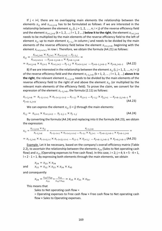
169

If j < i+l, there are no overlapping main elements the relationship between the elements 𝑥𝑥𝑝𝑝𝑖𝑖 and 𝑥𝑥𝑝𝑝+𝑇𝑇,𝑖𝑖+𝑘𝑘 has to be formulated as follows: if we are interested in the relationship between the element 𝑥𝑥𝑝𝑝𝑖𝑖 (i, j = 1, 2, … , n; i < j) of the reverse efficiency field and the element 𝑥𝑥𝑝𝑝+𝑇𝑇,𝑖𝑖+𝑘𝑘 (k = 1, 2, …; l = 1, 2 ,…) below it to the right, the element 𝑥𝑥𝑝𝑝+𝑇𝑇,𝑖𝑖+𝑘𝑘 needs to be multiplied by the main elements of the reverse efficiency field to the left of element 𝑥𝑥𝑝𝑝𝑖𝑖 up to main element 𝑥𝑥𝑖𝑖–1,𝑖𝑖 in column j and needs to be divided by the main elements of the reverse efficiency field below the element 𝑥𝑥𝑝𝑝+𝑇𝑇,𝑖𝑖+𝑘𝑘, beginning with the element 𝑥𝑥𝑝𝑝+𝑇𝑇,𝑝𝑝+𝑇𝑇+1 in row i. Therefore, we obtain the formula (A4.21) as follows:

𝑥𝑥𝑝𝑝𝑖𝑖 =𝑥𝑥𝑝𝑝+𝑇𝑇,𝑖𝑖+𝑘𝑘 × 𝑥𝑥𝑝𝑝,𝑝𝑝+1 × 𝑥𝑥𝑝𝑝+1,𝑝𝑝+2 … 𝑥𝑥𝑖𝑖–1,𝑖𝑖

𝑥𝑥𝑝𝑝+𝑇𝑇,𝑝𝑝+𝑇𝑇+1 … 𝑥𝑥𝑖𝑖+𝑘𝑘–2,𝑖𝑖+𝑘𝑘–1 × 𝑥𝑥𝑖𝑖+𝑘𝑘–1,𝑖𝑖+𝑘𝑘=

= 𝑥𝑥𝑝𝑝+𝑇𝑇,𝑖𝑖+𝑘𝑘 × 𝑥𝑥𝑝𝑝,𝑝𝑝+1 × 𝑥𝑥𝑝𝑝+1,𝑝𝑝+2 … 𝑥𝑥𝑖𝑖–1,𝑖𝑖 × 𝑥𝑥𝑝𝑝+𝑇𝑇+1,𝑝𝑝+𝑇𝑇 … 𝑥𝑥𝑖𝑖+𝑘𝑘–1,𝑖𝑖+𝑘𝑘–2 × 𝑥𝑥𝑖𝑖+𝑘𝑘,𝑖𝑖+𝑘𝑘–1 (A4.22)

8) If we are interested in the relationship between the element 𝑥𝑥𝑝𝑝𝑖𝑖 (i, j = 1, 2, …, n; i < j)of the reverse efficiency field and the element 𝑥𝑥𝑝𝑝–𝑇𝑇,𝑖𝑖+𝑘𝑘 (k = 1, 2, … ; l = 1, 2, …) above it to the right, the relevant element 𝑥𝑥𝑝𝑝–𝑇𝑇,𝑖𝑖+𝑘𝑘 needs to be divided by the main elements of the reverse efficiency field to the right of and above the element 𝑥𝑥𝑝𝑝𝑖𝑖 (or multiplied by the relevant main elements of the efficiency field). To prove the claim, we convert for the expression of the element 𝑥𝑥𝑝𝑝–𝑇𝑇,𝑖𝑖+𝑘𝑘, the formula (2.11) as follows:

𝑥𝑥𝑝𝑝–𝑇𝑇,𝑖𝑖+𝑘𝑘 = 𝑥𝑥𝑝𝑝–𝑇𝑇,𝑝𝑝–𝑇𝑇+1 × 𝑥𝑥𝑝𝑝–𝑇𝑇+1,𝑝𝑝–𝑇𝑇+2 … 𝑥𝑥𝑝𝑝–1,𝑝𝑝 × 𝑥𝑥𝑝𝑝,𝑝𝑝+1 … 𝑥𝑥𝑖𝑖–1,𝑖𝑖 × 𝑥𝑥𝑖𝑖,𝑖𝑖+1 … 𝑥𝑥𝑖𝑖+𝑘𝑘–2,𝑖𝑖+𝑘𝑘–1 ×𝑥𝑥𝑖𝑖+𝑘𝑘–1,𝑖𝑖+𝑘𝑘 (A4.23)

We can express the element 𝑥𝑥𝑝𝑝𝑖𝑖 (i < j) through the main elements:

𝑥𝑥𝑝𝑝,𝑖𝑖 = 𝑥𝑥𝑝𝑝,𝑝𝑝+1 × 𝑥𝑥𝑝𝑝+1,𝑝𝑝+2 … 𝑥𝑥𝑖𝑖–2,𝑖𝑖–1 × 𝑥𝑥𝑖𝑖–1,𝑖𝑖 (A4.24)

By converting the formula (A4.24) and replacing into it the formula (A4.23), we obtain the expression:

𝑥𝑥𝑝𝑝𝑖𝑖 =𝑥𝑥𝑝𝑝–𝑇𝑇,𝑖𝑖+𝑘𝑘 × 𝑥𝑥𝑝𝑝𝑖𝑖𝑥𝑥𝑝𝑝–𝑇𝑇,𝑖𝑖+𝑘𝑘

=𝑥𝑥𝑝𝑝–𝑇𝑇,𝑖𝑖+𝑘𝑘

𝑥𝑥𝑝𝑝–𝑇𝑇,𝑝𝑝–𝑇𝑇+1 × 𝑥𝑥𝑝𝑝–𝑇𝑇+1,𝑝𝑝–𝑇𝑇+2 … 𝑥𝑥𝑝𝑝–1,𝑝𝑝 × 𝑥𝑥𝑖𝑖,𝑖𝑖+1 … 𝑥𝑥𝑖𝑖+𝑘𝑘–2,𝑖𝑖+𝑘𝑘–1 × 𝑥𝑥𝑖𝑖+𝑘𝑘–1,𝑖𝑖+𝑘𝑘=

= 𝑥𝑥𝑝𝑝–𝑇𝑇,𝑖𝑖+𝑘𝑘 × 𝑥𝑥𝑝𝑝–𝑇𝑇+1,𝑝𝑝–𝑇𝑇 × 𝑥𝑥𝑝𝑝–𝑇𝑇+2,𝑝𝑝–𝑇𝑇+1 … 𝑥𝑥𝑝𝑝,𝑝𝑝–1 × 𝑥𝑥𝑖𝑖+1,𝑖𝑖 … 𝑥𝑥𝑖𝑖+𝑘𝑘–1,𝑖𝑖+𝑘𝑘–2 × 𝑥𝑥𝑖𝑖+𝑘𝑘,𝑖𝑖+𝑘𝑘–1 (A4.25)

Example. Let it be necessary, based on the company’s overall efficiency matrix (Table 2.2), to ascertain the relationship between the elements 𝑥𝑥24 (Sales to Net operating cash flow) and 𝑥𝑥15 (Operating expenses to Free cash flow). In this case, i = 2; j = 4; k = 5 - 4 = 1, l = 2 - 1 = 1. By expressing both elements through the main elements, we obtain

𝑥𝑥24 = 𝑥𝑥23 × 𝑥𝑥34 and 𝑥𝑥15 = 𝑥𝑥12 × 𝑥𝑥23 × 𝑥𝑥34 × 𝑥𝑥45

and consequently

𝑥𝑥24 = 𝑥𝑥15×𝑥𝑥24𝑥𝑥15

= 𝑥𝑥15𝑥𝑥12×𝑥𝑥45

= 𝑥𝑥15 × 𝑥𝑥21 × 𝑥𝑥54.

This means that Sales to Net operating cash flow = = Operating expenses to Free cash flow × Free cash flow to Net operating cash flow × Sales to Operating expenses.

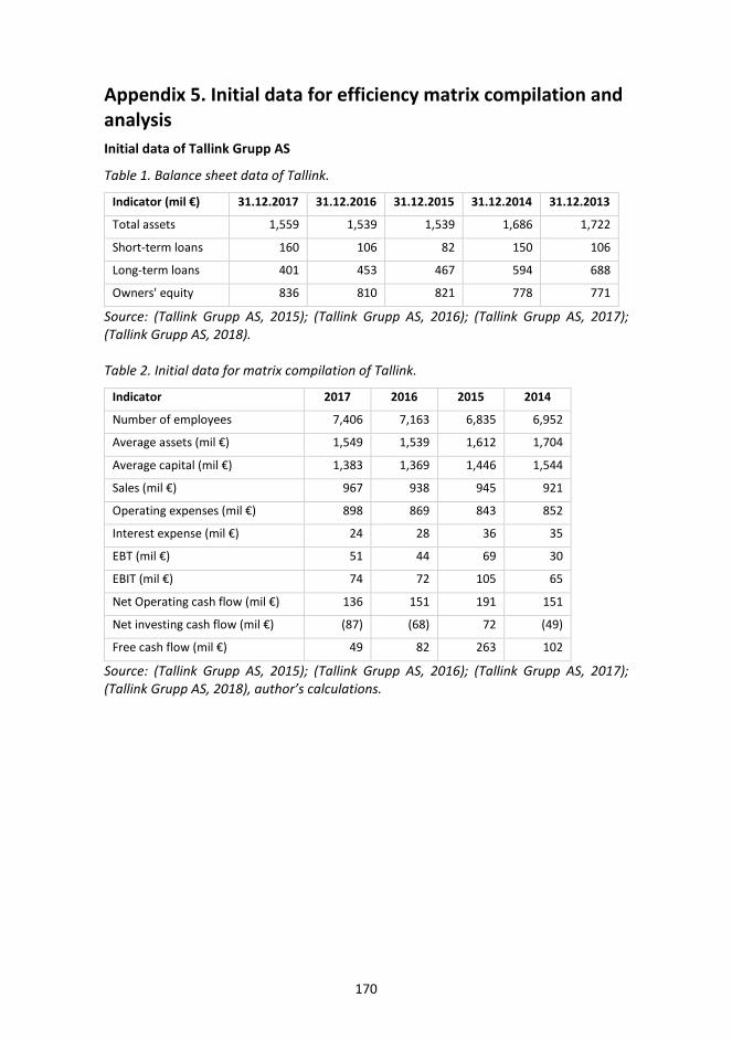
170

Appendix 5. Initial data for efficiency matrix compilation and analysis Initial data of Tallink Grupp AS

Table 1. Balance sheet data of Tallink.

Indicator (mil €) 31.12.2017 31.12.2016 31.12.2015 31.12.2014 31.12.2013

Total assets 1,559 1,539 1,539 1,686 1,722

Short-term loans 160 106 82 150 106

Long-term loans 401 453 467 594 688

Owners' equity 836 810 821 778 771

Source: (Tallink Grupp AS, 2015); (Tallink Grupp AS, 2016); (Tallink Grupp AS, 2017); (Tallink Grupp AS, 2018).

Table 2. Initial data for matrix compilation of Tallink.

Indicator 2017 2016 2015 2014

Number of employees 7,406 7,163 6,835 6,952

Average assets (mil €) 1,549 1,539 1,612 1,704

Average capital (mil €) 1,383 1,369 1,446 1,544

Sales (mil €) 967 938 945 921

Operating expenses (mil €) 898 869 843 852

Interest expense (mil €) 24 28 36 35

EBT (mil €) 51 44 69 30

EBIT (mil €) 74 72 105 65

Net Operating cash flow (mil €) 136 151 191 151

Net investing cash flow (mil €) (87) (68) 72 (49)

Free cash flow (mil €) 49 82 263 102

Source: (Tallink Grupp AS, 2015); (Tallink Grupp AS, 2016); (Tallink Grupp AS, 2017); (Tallink Grupp AS, 2018), author’s calculations.

171

Initial data of Viking Line Abp

Table 3. Balance sheet data of Viking Line.

Indicator (mil €) 31.12.2017 31.12.2016 31.12.2015 31.12.2014 31.12.2013

Total assets 485 506 528 533 530

Short-term loans 24 24 24 24 15

Long-term loans 127 151 174 198 221

Owners' equity 224 223 226 213 189

Source: (Viking Line Abp, 2015); (Viking Line Abp, 2016); (Viking Line Abp, 2017); (Viking Line Abp, 2018).

Table 4. Initial data for matrix compilation of Viking Line.

Indicator 2017 2016 2015 2014

Number of employees 2,048 2,046 2,735 2,797

Average assets (mil €) 495 517 530 532

Average capital (mil €) 386 410 429 430

Sales (mil €) 523 520 531 527

Operating expenses (mil €) 514 508 505 514

Interest expense (mil €) 4 5 5 6

EBT (mil €) 7 10 23 32

EBIT (mil €) 11 14 28 38

Net Operating cash flow (mil €) 37 36 55 38

Net investing cash flow (mil €) (31) (11) (8) (5)

Free cash flow (mil €) 6 26 47 33

Source: (Viking Line Abp, 2015); (Viking Line Abp, 2016); (Viking Line Abp, 2017); (Viking Line Abp, 2018), author’s calculations.

Table 5. Initial data and its dynamics for the compilation of Viking Line’s overall efficiency matrix.

Source: (by the author).

172

Table 6. Overall efficiency matrix of Viking Line.

Source: (by author).

173

List of Publications (1) Papers in international journals and books

Gofaizen, M., Siimann, P., & Alver, J. (2016). Profit per Employee Analysis (based on four major Estonian supermarket chains in 2010–2014). Advances in Economics, Business and Management Research(27), 79–89. (ETIS 3.1.)

Lohk, P.; Siimann, P. (2016). Predicting the Risk of Encountering Financial Difficulties by the Example of Estonian Municipalities. Advances in Economics, Business and Management Research(27), 297−306. (ETIS 3.1.)

Siimann, P., & Alver, J. (2015). On using an efficiency matrix in analysing profit per employee (on the basis of the Estonian SME software sector). Zeszyty Teoretyczne Rachukowości, 84(140), 195−215. (ETIS 1.2.)

Vaarmets, J.; Siimann, P. (2014). The impact of subsidies received on companies' financial ratios (by the example of medium-sized Estonian food companies from 2005–2012). International Conference on Accounting, Auditing, and Taxation (ICAAT 2014), Tallinn: DEStech Publications, Inc, 122−132. (ETIS 3.1.)

Siimann, P. (2011). Ratio classifications for financial statements analysis. Journal of International Scientific Publications: Economy & Business, 5, 127–140. (ETIS 1.2.)

(2) Conference proceedings

Siimann, P.; Alver, J. (2015). Profit per employee analysis (on the basis of Estonian SME software sector). Doctoral Summer School 2015, Pühajärve, Estonia, 3.–6.08.2015. (ETIS 3.4.)

Vaarmets, J.; Siimann, P. (2014). The impact of subsidies received on companies' financial ratios (by the example of medium-sized Estonian food companies from 2005–2012). Abstract. Accounting, Auditing, and Taxation, ICAAT 2014 Abstracts (pp. 14−15). Tallinn: Tallinna Tehnikaülikooli Kirjastus. (ETIS 5.2.)

Siimann, P. (2013). Ühe töötaja teenitud kasumi analüüsimisest efektiivsusmaatriksi põhjal (Eesti IKT sektori näitel). Audit, maksud, raamatupidamine ja majandusanalüüs II (pp 80−90). Tallinn: Tallinna Tehnikaülikooli Kirjastus. (ETIS 3.5.)

Siimann, P. (2012). Majandusaasta aruannete esitamiskohustusest Euroopa riikide näitel. In J. Alver, & K. Paldrok (Ed.), Audit, maksud, raamatupidamine ja majandusanalüüs (p. 94−102). Tallinn: Tallinna Tehnikaülikooli Kirjastus. (ETIS 3.5.)

Siimann, P. (2011). An overview of the theoretical fundamentals and developments of the efficiency matrix. Business Analysis, Accounting, Taxes and Auditing (pp. 256–268). Tallinn: Tallinn University of Technology. (ETIS 3.4.)

Siimann, P. (2010). Kvantitatiivsete uurimismeetodite kasutamisest finantsaruannete analüüsimisel. Raamatupidamiselt majandusarvestusele III, (pp. 71–77). Tallinn: Tallinna Tehnikaülikool. (ETIS 3.5.)

Siimann, P. (2009). Finantsaruannete analüüsimise arengust enne Teist maailmasõda. Raamatupidamiselt majandusarvestusele II (pp. 89–92). Tallinn: Tallinna Raamatutrükikoda, 89–92. (ETIS 3.4.)

174

Siimann, P. (2008). A review of ratio classifications for financial statement analysis. Business analysis, accounting, taxes and auditing: proceedings of the conference, 6–7 November 2008 (pp. 174–179). Tallinn: Tallinn University of Technology (ETIS 3.4.)

Siimann, P. (2008). Analüüs ja selle rakendamine. Business analysis, accounting, taxes and auditing: proceedings of the conference 6–7 November 2008 (pp. 365–368). Tallinn University of Technology (ETIS 3.4.)

Kitvel, E.; Siimann, P. (2007). Ettevõtte majandustulemuste võrdlev analüüs (Eesti Statistikaameti koostatud tegevusala ettevõtete alusel). Raamatupidamiselt majandusarvestusele I (pp. 71–79). Tallinn: Tallinna Tehnikaülikool. (ETIS 3.5.)

Siimann, P.; Kitvel, E. (2007). Comparative analysis of financial statements using ratios. BAA Annual Conference 2007, London, 3–5 April 2007 (p. 192). London: British Accounting Association. (ETIS 5.2.)

Siimann, P.; Mand, U. (2006). Klientide kasumlikkuse mõõtmine. Konverentsikogumik: Accounting, Taxes and Audit. Arvestus, maksud ja auditeerimine. Tallinn, 26 –27 October 2006 (pp. 287–292). Tallinn: Tallinna Tehnikaülikooli Kirjastus. (ETIS 3.4.)

175

Curriculum vitae Personal data

Name: Paavo Siimann Date of birth: 20 November 1975 Place of birth: Tallinn, Estonia Citizenship: Estonia

Contact data E-mail: paavo.siimann@gmail.com

Education 2005–2018 Tallinn University of Technology – PhD (Business Administration) 1999–2001 Tallinn University of Technology – MSc (Business Administration) 1994–1999 Tallinn University of Technology – Economist (Accounting) 1991–1994 Gustav Adolf Grammar School – Secondary education

(mathematics-physics) Language competence

Estonian Mother tongue English Proficient Russian Intermediate Finnish Intermediate

Professional employment 2017– Tallinn University of Technology, School of Business and

Governance, Department of Business Administration – Lecturer (0.25)

2011–2017 Circle K Eesti AS (former Statoil Fuel & Retail Eesti AS, Eesti Statoil AS) – Finance and Control Director, Member of Management Board

2005–2011 AstraZeneca Eesti OÜ – Finance Manager 2002–2005 GlaxoSmithKline Eesti Eesti OÜ – Financial Analyst 2002–2016 Tallinn University of Technology, School of Economics and

Business Administration, Department of Accounting, Chair of Management Accounting – Lecturer (0.25)

2001–2002 Tridens – Product Manager 2000–2002 Tallinn University of Technology, School of Economics and

Business Administration, Department of Accounting, Chair of Management Accounting – Assistant (0.50)

176

Elulookirjeldus Isikuandmed

Nimi: Paavo Siimann Sünniaeg: 20. november 1975Sünnikoht: Tallinn, Eesti Kodakondsus: Eesti

Kontaktandmed E-post: paavo.siimann@gmail.com

Hariduskäik 2005–2018 Tallinna Tehnikaülikool – PhD (ärikorralduses) 1999–2001 Tallinna Tehnikaülikool – MSc (ärikorralduses) 1994–1999 Tallinna Tehnikaülikool – ökonomist (majandusarvestuses) 1991–1994 Gustav Adolfi gümnaasium – keskharidus (matemaatika-

füüsika süvaõpe) Keelteoskus

Eesti keel emakeel Inglise keel kõrgtase Vene keel kesktase Soome keel kesktase

Teenistuskäik 2017– Tallinna Tehnikaülikooli majandusteaduskonna ärikorralduse

instituut – lektor (0,25) 2011–2017 Circle K Eesti AS (endine Statoil Fuel & Retail Eesti AS, Eesti

Statoil AS) – finantsdirektor, juhatuse liige 2005–2011 AstraZeneca Eesti OÜ – finantsjuht 2002–2005 GlaxoSmithKline Eesti Eesti OÜ – finantsanalüütik 2002–2016 Tallinna Tehnikaülikooli majandusteaduskonna

majandusarvestuse instituudi juhtimisarvestuse õppetool – lektor (0,25)

2001–2002 Tridens – tootejuht 2000–2002 Tallinna Tehnikaülikooli majandusteaduskonna

majandusarvestuse instituudi juhtimisarvestuse õppetool – assistent (0,50)