U.S. monetary policy indicators and international stock returns: 1970–2001

International Review of Financial Analysis

13 (2004) 543–558

U.S. monetary policy indicators and international

stock returns: 1970–2001

Thomas Manna,*, Robert J. Atrab, Richard Dowenc

aSchool of Business and Economics, Lynchburg College, Lynchburg, VA 24501, USAbFinance Department, College of Business, Lewis University, Romeoville, IL, USA

cFinance Department, College of Business, Northern Illinois University, DeKalb, IL 60115, USA

Abstract

It is documented in the literature that U.S. and many international stock returns series are

sensitive to U.S. monetary policy. Using monthly data, this empirical study examines the short-term

sensitivity of six international stock indices (the Standard & Poor 500 [S&P] Stock Index, the

Morgan Stanley Capital International [MSCI] European Stock Index, the MSCI Pacific Stock Index,

and three MSCI country stock indices: Germany, Japan, and the United Kingdom) to two major

groups of U.S. monetary policy indicators. These two groups, which have been suggested by recent

research to influence stock returns, are based on the U.S. discount rate and the federal funds rate. The

first group focuses on two binary variables designed to indicate the stance in monetary policy. The

second group of monetary indicators involves the federal funds rate and includes the average federal

funds rate, the change in the federal funds rate, and the spread of the federal funds rate to 10-year

Treasury note yield. Dividing the sample period (1970–2001) into three monetary operating

regimes, we find that not all policy indicators influence international stock returns during all U.S.

monetary operating periods or regimes. Our results imply that the operating procedure and/or target

vehicle used by the Federal Reserve Board (Fed) influences the efficacy of the policy indicator. We

suggest caution in using any monetary policy variable to explain and possibly forecast U.S. and

international stock returns in all monetary conditions.

D 2004 Elsevier Inc. All rights reserved.

Keywords: U.S. monetary policy indicators; International stock returns; MSCI; S&P

1057-5219/$ - see front matter D 2004 Elsevier Inc. All rights reserved.

doi:10.1016/j.irfa.2004.02.025

* Corresponding author.

E-mail addresses: [email protected] (T. Mann), [email protected] (R.J. Atra), [email protected]

(R. Dowen).

T. Mann et al. / International Review of Financial Analysis 13 (2004) 543–558544

1. Introduction

Recent research suggests that certain groups of monetary policy indicators or

variables based on the federal funds rate or the discount rate have the ability to help

explain and/or possibly forecast U.S. and international stock returns. Since equities

represent claims on future profits of firms, which, in turn, are generated from future

economic output, changes in monetary policy to raise or lower interest rates should

measurably impact stock returns. The standard discounted cash flow model posits that

increasing interest rates should adversely affect stock returns while decreasing interest

rates should positively impact stock returns. Changes in interest rates will be felt directly

through the discount rate used in the model. An additional indirect impact will flow

from the anticipated increase or decrease of cash flows due to changed economic

activity.

The focus of this study is to empirically examine the sensitivity of several

international stock total return series to Federal Reserve Board (Fed) monetary policy

as reflected by two groups of monetary indicators controlled by the Fed: the federal

funds rate and the U.S. discount rate. We are particularly interested if the influences on

stock returns by these monetary indicators are robust to different historical and current

operating procedures and/or target variables used by the Fed to control the money

supply.

Bernanke and Blinder (1992, p. 902) suggest that monetary policy affects aggregate

demand through the demand for bank credit. They state, ‘‘. . .we entertain the idea that the

federal funds rate (or the spread between the funds rate and some alternative open-market

rate) is an indicator of Federal Reserve policy.’’ Extending this notion, Patelis (1997) and

Thorbecke (1997) analyze the ability of several federal funds variables to forecast stock

returns.

Applying VAR methodology to stock return data supplied by CRSP for the sample

period 1953–1990, Thorbecke (1997) finds a statistically significant negative relationship

between changes in the federal funds rate and industry and size portfolios. Thorbecke (p.

648) also presents additional evidence from an event study that ‘‘. . .there is a statisticallysignificant negative relation between policy-induced changes in the funds rate and changes

in the DJIA (Dow Jones Industrial Average) and the DJCA (Dow Jones Composite

Average).’’

With a multifactor VAR model, Patelis (1997) examines the impact of the federal

funds rate and the spread of the federal funds rate to the 10-year Treasury note rate on

monthly NYSE value-weighted excess stock returns obtained from CRSP. The sample

period ranges from January 1962 to November 1994 with analysis focused on

monthly, quarterly, annual, and biennial horizons. Patelis finds the federal funds rate

and the federal funds spread to be highly significant (P values of .000 and .017,

respectively).

In a different approach to measuring monetary policy, Jensen, Mercer, and Johnson

(1996) use a binary variable to indicate the direction of monetary policy. They define

monetary policy as either expansive or restrictive based on the direction of change in the

discount rate. Using time series regressions on monthly and quarterly data over a sample

period from February 1954 through December 1991, they find that security prices are

T. Mann et al. / International Review of Financial Analysis 13 (2004) 543–558 545

sensitive to macroeconomic variables as a function of the Fed monetary policy. For ease of

description, we label this binary variable approach to describing monetary policy as a

discount rate regime (DRR).

Using t tests, F tests, and time series regressions, Conover, Jensen, and Johnson (1999a,

1999b) and Johnson, Beutow, and Jensen (1999) extend the use of the DRR policy

variable to analyze monthly international stock and mutual fund returns. Using a sample

period that extends from January 1970 through December 1995, Conover et al. (1999a,

1999b) find that stock returns are generally higher during periods of expansive U.S. as

well as local monetary policy. In Johnson et al. (1999), the sample period runs from

January 1976 through September 1998.

Using the DRR methodology over the period from January 1970 to December

2001, we count nine distinct periods of increasing and eight decreasing discount rates.

In addition, during this same period, we observe the Fed using several distinct

operating procedures and/or target variables to implement monetary policy. To describe

a period when the Fed uses a procedure or variable to control the money supply,

Ogden (1990) suggests the notion of a monetary operating regime. He defines a

monetary operating regime as a period when the Fed uses a distinct set of procedures

and/or target variables to implement the desired monetary policy (restrictive or

expansive). With this definition, a monetary operating regime or period is thus

differentiated from monetary policy or stance, and together they constitute the current

monetary condition.

We examine two questions in this study. First, are U.S. and international stock index

returns consistently sensitive to the two groups of monetary policy indicators in light of the

several historical monetary operating regimes evident from 1970 to 2001? Second, are any

of these monetary policy variables statistically important during the current monetary

operating regime of specifically targeting the federal funds rate and thus can be used as a

current indicator of monetary policy?

This study extends previous research in several ways. First, it provides a side-by-side

comparison of the two groups of monetary indicators that are most prevalent in current

research. Second, this study examines the impact of these various monetary indicators

across several distinct monetary operating regimes. Third, this study extends analysis

through December 2001.

Section 2 outlines the definition of a monetary operating regime, while Section 3

describes data and methodology used this analysis. We present our empirical results in

Section 4 and conclude our analysis in Section 5.

2. Monetary operating regimes

Ogden (1990) differentiates monetary policy from monetary operating regime. The

terms monetary operating regime and monetary operating period indicate the period

during which the FED uses a unique set of procedures and variables to manage the

money supply. One such example is the period from October 1979 to October 1982,

when the FED specifically targeted nonborrowed reserves to determine the credit needs

of the economy. Monetary policy then refers to the directive of the Fed to maintain a


restrictive or expansive monetary environment. Our measure of the monetary operating

regime will be the period during which the FED uses a different target or sets of targets

to guide policy.

We delineate the breakpoints in monetary operating regimes based on two criteria.

The first criterion uses announcements and/or direct actions of the Fed. We accept at

face value the pronouncements of the Fed when they indicate a change in operating

procedure or targeting variables. The change to targeting monetary aggregates in

October 1979 and the use of the federal funds rate as a target variable beginning in

August 1987 provide two distinct changes from previous procedure. The dates become

two of our breakpoints. Our second criterion is based on historical narratives (e.g.,

Meulendyke, 1998).

With these criteria, we demarcate three major operating periods from January 1970 to

December 2001. The first period runs from January 1970 to October 1979. It was during

this period that the FED introduced the use of the federal funds rate to help guide

monetary policy. Meulendyke (1998, pp. 44–45) describes FED operating procedure as:

‘‘. . .until October 1979 the framework used by the FOMC for guiding open market

operations generally included setting a monetary objective and encouraging the federal

funds rate to move gradually up or down if money was exceeding or falling short of the

objective.’’

In late October 1979, the FED dramatically changed its operating procedures to

targeting nonborrowed reserves as the policy variable. This action of the FED starts the

second period at November 1979. The FED continued to target other monetary aggregates

until early 1984 when it gradually moved to using other economic information. Period 2

covers the period from November 1979 to August 1987. Meulendyke (1998, p. 53)

describes operating conditions from approximately 1984 to 1987 as follows: ‘‘Policy

decisions were also guided by information on economic activity, inflation, foreign

exchange developments, and financial market conditions.’’

With Alan Greenspan as the new FED chairman, the FED began focusing more on

the federal funds rate as the key policy variable. The shift was marked by the turmoil

of the severe market decline in October 1987. While we begin the third major

operating period in September 1987, we recognize that the shift to using the federal

funds rate as a direct indicatory of monetary policy continued into 1988. Period 3

extends through December 2001. The monetary operating periods or regimes are

summarized in Table 1.

Table 1

Major monetary operating regimes/periods: January 1970 to December 2001

Monetary

operating

period

Time period Operating guidance/procedure(s)

1 January 1970 to October 1979 Federal funds rate; short-term growth rates in money supply

2 November 1979 to August 1987 Begin period by targeting monetary aggregates and slowly

move to using inflation and general economic variables as

guidelines

3 September 1987 to December 2001 Federal funds rate as the target variable


3. Methodology and data

We hypothesize that the efficacy of the sensitivity of stock returns to various policy

indicators may be based on the operating procedure and/or target variables used by the Fed

to operate monetary policy. Different operating procedures or target variables may render

certain indicators ineffective to influencing stock returns, hence the need to examine the

robustness of the indicators by monetary operating regimes. Specifically, this study seeks

to examine the sensitivity of monthly excess returns of U.S. and major international stock

indices to five specific monetary policy variables during three separately defined monetary

operating regimes over the sample period 1970–2001.

3.1. Data

The set of federal funds rate monetary policy variables include the average federal

funds rate, the change in the federal funds rate and the spread of the federal funds rate to

the 10-year Treasury note yield. The discount rate monetary policy indicators include a

binary variable defined by changes in the discount rate (DRR) and a combination binary

variable defined by changes in the discount rate with a substitution of changes in the

federal funds target rate when the latter is used by the Fed as a target variable. We define

that latter variable as a monetary policy regime (MPR) variable.

We examine three monetary variables based on the federal funds rate as suggested and

used by Bernanke and Blinder (1992), Patelis (1997), and Thorbecke (1997). The first is

the monthly average federal funds rate (FF). The second is the first difference in the

average federal funds rate (ChgFF). This variable is calculated as the monthly average

federal funds rate in month t minus the monthly average federal funds rate in month t� 1,

where t is a monthly counter. The third variable is the federal fund spread (FFsprd). It is

calculated as the monthly average federal funds rate minus the monthly average 10-year

Treasury note yield, all in period t.

We examine two monetary policy indicators based on the discount rate. The first

indicator is a zero–one binary variable to indicate the direction of monetary policy

evidenced by the FED increasing or decreasing the discount rate (Jensen et al., 1996). A

change in direction of the discount rate as of the beginning of the month determines if a

decrease or increase has occurred. We define the binary variable (DRR) with a value of

one beginning with a rate increase and continuing until a rate decrease. The binary variable

then takes on value of zero beginning with a rate decrease and continuing until a rate

increase. A restrictive monetary policy occurs when the discount rate is increasing; an

expansive monetary policy occurs when the discount rate is lowered.

We extend this idea by incorporating the federal funds target rate at the beginning of the

month when this variable is available and published. We do so based on the fact that from

1975 to 1979 and from September 1987 to present the Fed has used the federal funds rate

as a target variable. We use the change in the federal funds target rate to determine the

direction of monetary policy and substitute the results into the DRR variable. Values of

one indicate a restrictive monetary policy and zero an expansive policy. This creates a

combination binary variable that we posit should more accurately reflect Fed monetary

policy as expansive or restrictive. We denote this new binary variable as an MPR variable.


The stock index rate of return series are supplied by Ibbottson and Associates (Chicago,

IL) and Morgan Stanley Capital International (MSCI) from their website. These indices are

widely used by researchers, portfolio managers, and the public. The indices (with

mnemonic variable names used in this study in parentheses) are: Standard & Poor’s 500

Stock Total Return Index (S&P 500), MSCI European Stock Total Return Index (Eur),

MSCI Pacific Stock Total Return Index (Pac), MSCI Germany Total Return Index (Ger),

MSCI Japan Total Return Index (Jap), and the United Kingdom MSCI Total Return Index

(UK).1 The country indices are selected based on their weight in the area index. All indices

are value weighted. All return series are denominated in dollars to give the viewpoint of an

unhedged U.S. investor. Each return series is converted to an excess return series by

subtracting the U.S. 30-day T-bill rate (also supplied by Ibbotson). Monthly returns are

examined in this study simply to be comparable to many other studies. The sample period

extends from January 1970 through December 2001.

To control for economic activity, we analyze and include several variables. Following

on results from Brocato and Steed (1998) and Siegel (1991), we construct a binary variable

based on the business cycle. Using data from the National Bureau of Economic Research

(NBER), the binary variable (BusCycle) is assigned a value of 1 if the economy is

officially in recession as of the beginning of the month and 0 otherwise. We view this

variable as a simple and unambiguous way to describe the state of the U.S. economy. In

Table 2, we present results from sorting stock returns based on whether the U.S. economy

is in recession or expansion. Except for UK returns, the BusCycle variable offers

explanatory power to predict and explain stock returns.

We also examine a set of Fama and French (1989) variables to control for economic

activity: a dividend yield variable, two default spread variables, and a term variable. Using

data supplied by Ibbotson, the dividend yield variable (DivYld) is calculated as the sum of

the income returns on the S&P 500 index for the prior 11 months plus the current month

divided by the end of month price of the index for the current month (Fama, 1990). We

consider two different default variables suggested by the literature. Default variable 1

(DEF1) is constructed as the difference of the Baa corporate bond rate and the Aaa

corporate bond rate (Fama, 1990). We construct the second default variable (DEF2) as the

difference of the Baa corporate bond rate and the 10-year Treasury note yield (Jensen et

al., 1996). Finally, we include a term variable (Term) that is measured as the 3-month T-

bill rate minus the 10-year Treasury note yield. However, since this variable can also

represent the stance in monetary policy, the use of Term as a control variable is

problematic. The monthly interest rate data series (federal funds rate, 10-year Treasury

note yield, Aaa and Baa corporate bond yield, 3-month Treasury bill rate) and dates of

1 The S&P 500 stock index is constructed as a market value-weighted benchmark of 500 stocks determined

by their market value. Total return includes dividend plus capital appreciation. The MSCI stock index returns for

Europe, the Pacific, and countries are calculated based on achieving 60% coverage of the total market

capitalization for each country market with certain exceptions. A list of exceptions can be found at the Morgan

Stanley Capital Markets website www.msci.com. Country markets comprising the Europe index include Austria,

Belgium, Denmark, Finland, France, Germany, Ireland, Italy, Netherlands, Norway, Portugal, Spain, Sweden,

Switzerland, and the United Kingdom. Country markets comprising the Pacific index include Australia, Hong

Kong, Japan, New Zealand, and Singapore.

http:\\www.msci.com

http:\\www.msci.com

Table 2

Analysis of sensitivity of stock returns to U.S. business cycle

Obs Mean returns (%)

S&P 500 Eur Ger UK Pac Jap

BusCycle = 0 318 0.77 0.78 0.82 0.76 0.92 1.00

BusCycle = 1 66 � 0.69 � 0.73 � 0.99 0.01 � 1.61 � 1.55

Difference 1.46** 1.51** 1.81** 0.75 2.53** � 2.55**

The NBER determines the business cycle for the United States. If the NBER declares the United States is

officially in recession at the beginning of the month, a 1 is coded for BusCycle; otherwise, a 0 is coded. Stock

returns are sorted by recession or expansion and mean values are calculated. Returns are calculated as percent.

Significance is based on P value of a one-tailed t test.

**P< .05.


discount rate changes can be obtained from the St. Louis Federal Reserve Bank data bank

posted on the Internet. Federal funds targets are obtained from FRB press releases and

from Neal, Roley, and Sellon (1998).

3.2. Methodology

This study employs ordinary least squares with the monthly total excess return of a

stock index as the dependent variable regressed against each monetary indicator and an

economic activity control variable in a series of two regressions. Since our focus is on the

contemporary influence of these monetary policy variables on stock returns, the dependent

as well as independent variables are set to period t. The first regression encompasses the

entire sample period, 1970–2001. The second regression breaks up the sample period into

the three postulated major monetary operating periods using binary variables to represent

each period. Each binary variable equals 1 during the particular monetary operating period

(Pi) and 0 otherwise. In this manner, the sensitivity of each monetary indicator variable to

each stock index can be examined for the entire sample period and by monetary regime.

Using the S&P 500 index and the MPR variable as an example, we fit the following set of

equations:

SP 500t ¼ b0 þ b1MPRt þ b2BusCyclet þ et ð1Þ

SP 500t ¼ b0 þ b1½P1�MPRt� þ b2½P2�MPRt� þ b3½P3�MPRt�

þ b4BusCyclet þ et: ð2Þ

Similar to results in Jensen et al. (1996), Patelis (1997), and Thorbecke (1997), we

expect an overall negative relationship between the policy indicator and stock returns. In

general, over the entire sample period, if the discount rate or federal funds rate increases,

this should have a negative impact on stock returns on average. However, we do not

expect each indicator to be statistically significant during each operating period. Statistical

sensitivity of stock returns to a policy indicator may depend on the operating procedure

and/or target variable used by the Fed. This should be especially relevant during the

Table 3

Correlation between all variables

S&P 500 Eur Pac Ger Jap UK DRR MPR FF ChgFF FFsprd BusCycle Term DEF1 DEF2

Eur .6**

Pac .38** .56**

Aus .49** .52** .44**

Can .74** .58** .4**

Fr .47** .78** .45**

Ger .41** .78** .41**

Jap .32** .50** .98** .37**

Swe .45** .62** .43** .43** .38**

UK .52** .85** .43** .55** .37**

DRR � .17** � .16** � .17** � .09* � .16** � .16**

MPR � .19** � .17** � .17** � .13** � .16** � .16** .69**

FF � .13** � .15** � .12** � .11** � .10** � .12** .43** .30**

ChgFF � .18** � .18** � .07 � .14** � .05 � .15** .21** .26** .12**

FFsprd � .15** � .16** � .13** � .11** � .12** � .15** .54** .43** .71** .17**

BusCycle � .12** � .12** � .16** � .11** � .15** � .05 .10* � .02 .34** � .25** .34**

Term � .13** � .14** � .14** � .10** � .13** � .13** .54** .45** .53** .21** .93** .20**

DEF1 .11** .06 .11* .03 .11* .11* � .18** � .23** .53** � .18** .06 .27** � .13**

DEF2 .17** .11** .16** .07 .16** .14** � .45** � .49** � .06 � .31** � .15 .24** � .24** .62**

DivYld � .08 � .03 � .02 � .02 � .03 � .01 .16** .05 .66** � .03 .16** .25** � .02 .65** � .02

*P< .10.

**P < .05.

T.Mannet

al./Intern

atio

nalReview

ofFinancia

lAnalysis

13(2004)543–558

550


current period of targeting the federal funds rate where we do not expect stock returns to

be sensitive to the DRR binary variable.

4. Empirical results

4.1. Correlation results

Table 3 contains the correlations between the various stock return indices (S&P 500,

Eur, Pac, Ger, Jap, and UK), monetary policy indicators (DRR, MPR, FF, ChgFF, and

FFsprd), and our several proxies for economic activity (DivYld, DEF1, DEF2, Term, and

BusCycle). Several results are important. First, all five monetary indicators are negatively

correlated with stock returns and are statistically significant with P values less than .05.

The exception is the correlation between the Pac and Jap index stock returns and the

ChgFF policy indicator. Second, our primary indicator of U.S. economic activity is also

significantly correlated with international stock returns except for UK returns. This leads

us to believe that this variable may work well to represent U.S. economic activity in the

regression equations. In fact, in results not reported here, we find most MSCI country

stock return indices are significantly correlated with the U.S. business cycle indicator

(BusCycle). Third, we notice some high correlations among the Fama–French economic

variables (DivYld, Term, DEF1, DEF2) themselves and to the BusCycle variable. Fourth,

we notice a high degree of correlation between some of the economic control variables and

the monetary policy indicators. This makes us wary of issues of multicollinearity in the

Table 4

Regression analysis of DRR variables as a monetary policy indicator


Panel A. Analysis of impact of DRR across all monetary operating regimes

Constant 1.37** 1.36** 1.33** 1.64** 1.73** 1.84**

BusCycle � 1.27** � 1.32** � 1.64** � 0.52 � 2.28** � 2.28**

DRR � 1.45** � 1.41** � 1.23** � 2.10** � 1.94** � 2.01**

Adjusted R2 (%) 3.5 3.0 1.8 2.0 4.3 3.9

F value 7.9** 6.9** 4.6** 4.9** 9.6** 8.7**

DW 2.07 2.02 2.06 1.88 1.86 1.89

Panel B. Analysis of impact of DRR by monetary operating regime

Constant 1.35** 1.35** 1.32** 1.60** 1.75** 1.86**

BusCycle � 1.08* � 1.20* � 1.53* � .20 � 2.42** � 2.46**

P1�DRR � 2.07** � 1.34 � 1.06 � 2.67** � 1.64* � 1.65*

P2�DRR � 1.24 � 2.07* � 2.79** � 2.85** � 1.61 � 1.55

P3�DRR � 1.02* � 1.03 � .85 � 1.41 � 2.28** � 2.44**

Adjusted R2 (%) 3.5 3.1 1.9 1.9 3.9 3.5

F value 4.4** 4.1** 2.8** 2.8** 4.9** 4.5**

DW 2.07 2.03 2.08 1.89 1.86 1.89

*P< .10.

**P< .05.


regression equations. Resultantly, we will choose economic control variables based on the

following criteria from the correlation analysis: (1) statistical significance with stock

returns, (2) no or low collinearity with other control variables, and (3) no or low

collinearity with monetary policy indicators.

We notice that the dividend yield variable is not significantly correlated with stock

returns and as a result do not include DivYld as a control variable. In addition, we find that

the Term variable is highly correlated with all the other economic control variables as well

as the monetary policy indicators. Therefore, we exclude Term as a control variable. The

construction of Term variable appears to reflect monetary policy as well as economic

activity.

We note a high degree of correlation between default variables, DEF1 and DEF2, and

the binary monetary policy indicators based on the discount rate. By definition, DEF2 has

aspects of a yield curve variable, i.e., in that the difference is between a 20-year corporate

bond (Baa rating) and a 10-year Treasury note. Resultantly, we do not include either

default variable in our regression analyses of the discount rate-based binary policy

indicators. However, based on no or low correlation, we will use DEF2 as an economic

control variable with two policy indicators based on the Fed funds rate: the federal funds

rate (FF) and the spread of the federal funds rate to the 10-year Treasury note yield

(FFsprd). We eliminate DEF1 as an economic control variable based on the low and

nonsignificance with respect to the majority of the stock return series.

We observe that BusCycle is highly collinear with the policy indicators based on the

federal funds rate, but has little correlation with the discount rate based binary variables.

We use BusCycle as an economic control variable with the discount rate based binary

Table 5

Regression analysis of MPR variables as a monetary policy indicator


Panel A. Analysis of impact of MPR across all monetary operating regimes

Constant 1.55** 1.53** 1.52** 1.78** 1.92** 1.96**

BusCycle � 1.49** � 1.54** � 1.91** � .80 � 2.58** � 2.59**

MPR � 1.70** � 1.62** � 1.23** � 2.21** � 2.19** � 2.08**

Adjusted R2 (%) 4.5 3.7 1.5 2.3 5.0 4.1

F value 10.0** 8.4** 4.0** 5.0** 11.1** 9.2**

DW 2.07 2.02 1.91 1.89 1.87 1.89

Panel B. Analysis of impact of MPR by monetary operating regime

Constant 1.51** 1.49** 1.49** 1.74** 1.96** 1.99**

BusCycle � 1.29* � 1.35** � 1.64** � .62 � 2.75** � 2.75**

P1�MPR � 2.36** � 1.66** � 1.52* � 2.41** � 1.90** � 1.84**

P2�MPR � 1.34 � 2.80** � 2.93** � 2.88** � 1.72 � 1.60

P3�MPR � 1.20** � 1.17* � 1.05 � 1.79* � 2.63** � 2.49**

Adjusted R2 (%) 4.7 3.8 2.4 1.9 4.7 3.7

F value 5.7** 4.8** 3.4** 2.9** 5.7** 4.7**

DW 2.07 2.04 2.09 1.89 1.88 1.89

*P < .10.

**P < .05.


variables. We also choose to use BusCycle as an economic control variable with

regressions analyzing ChgFF.

In summary, we choose two variables to control for economic activity, BusCycle and

DEF2, and use them based on the premise of no or little correlation with the monetary

policy indicators but significant correlation with stock returns. BusCycle will be used with

the binary monetary policy indicators DRR, MPR, and ChgFF. DEF2 will be used with

regressions analyzing the impact of the federal funds rate (FF) and the spread of the federal

funds rate to the 10-year Treasury note yield (FFsprd).

4.2. Monetary indicators based on the discount rate

Results for monetary indicators based on the discount rate (DRR and MPR) are

presented in Tables 4 and 5, respectively. The adjusted R2 for all 12 equations ranges

from 1.8% to 4.7%. These are comparable to the monthly regression results from Fama

and French (1989) and Jensen et al. (1996). Generally, the BusCycle control variable is

statistically significant in all regression equations with the major exception of United

Kingdom excess index returns. In Table 4, we note that the DRR variable is statistically

significant across all monetary operating regimes (panel A). However, when we analyze

the importance by monetary operating regime (panel B), we find spotty results. For the

Table 6

Analysis of DRR variable using t tests by monetary operating periods



Panel A. All monetary periods: January 1970 to December 2001

DRR=0 216 1.20 1.18 1.10 1.57 1.42 1.52

DRR=1 168 � 0.35 � 0.33 � 0.25 � 0.57 � 0.70 � 0.66

Difference 1.55** 1.55** 1.35** 2.14** 2.12** 2.18**

Panel B. Monetary Period 1: January 1970 to October 1979

DRR=0 54 1.38 1.12 1.27 2.48 2.62 2.99

DRR=1 64 � 1.12 � 0.43 � 0.29 � 1.15 � 0.76 � 0.67

Difference 2.50** 1.55** 1.56* 3.63** 3.38** 3.66**

Panel C. Monetary Period 2: November 1979 to August 1987

DRR=0 67 1.49 2.09 1.98 2.26 2.66 2.84

DRR=1 27 � 0.21 � 1.71 � 1.92 � 1.31 � 0.57 � 0.42

Difference 1.70* 3.80** 3.90** 3.57** 3.23** 3.26**

Panel D: Monetary Period 3: September 1987 to December 2001

DRR=0 95 0.90 0.57 0.39 0.56 � 0.15 � 0.25

DRR=1 77 0.24 0.23 0.36 0.16 � 0.69 � 0.73

Difference 0.66 0.34 0.03 0.40 0.54 0.48

Monthly index total excess returns are sorted by DRR variable for the total sample period as well as for each

monetary operating period and a mean value is calculated. Returns are calculated as percent. Significance is based

on P value of a one-tailed t test.

*P< .10.

**P< .05.


U.S. stock index, DRR is strongly significant during Period 1, not significant during

Period 2, and marginally significant during Period 3. The DRR variable is not

significant during Period 3 for the European, German, and UK stock indices. For the

Pacific and Japan stock indices, DRR is highly significant during Period 3, not

significant during Period 2, and marginally significant during Period 1. We find no

consistent pattern.

The MPR variable is an extension of the DRR variable. With the MPR variable, the

S&P 500 and Pacific stock indices have higher R2 than with the DRR variable.

Comparing regression R2 using the DRR and MPR variables lead to mixed results. The

federal funds rate was used as a target variable from August 1974 through September

1979 during designated monetary operating Period 1. Additionally, during the current

monetary operating regime (Period 3), the Fed uses the federal funds rate as its target

variable. During monetary Period 2, the Fed did not use the federal funds rate as a

target variable but did use the discount rate as an informational indicator of monetary

stance. Because DRR and MPR are the same for Period 2, we should expect the

regression coefficients to be of the same sign, approximately equal and of the same

importance; they are. In Period 3, the MPR variable as compared to the DRR variable

becomes strongly significant for U.S. returns and becomes marginally significant for

Europe and UK returns.

We extend our analyses of the two binary monetary policy indicators by sorting the

monthly total excess returns for each index into periods of restrictive or expansive

Table 7

Analysis of MPR variable using t tests by monetary operating periods



Panel A. All monetary periods January 1970 to December 2001

MPR=0 216 1.28 1.25 1.20 1.63 1.47 1.50

MPR=1 168 � 0.39 � 0.36 � 0.32 � 0.57 � 0.69 � 0.56

Difference 1.67** 1.61** 1.52** 2.20** 2.16** 2.16**

Panel B. Monetary Period 1: January 1970 to October 1979

MPR=0 54 1.54 1.20 1.53 2.24 2.64 2.98

MPR=1 64 � 1.25 � 0.51 � 0.51 � 0.95 � 0.78 � 0.66

Difference 2.79** 1.71** 2.04** 3.19** 3.42** 3.64**

Panel C. Monetary Period 2: November 1979 to August 1987

Same results as for DRR variable. The Fed did not use the federal funds rate as a target variable during this

monetary operating period.

Panel D: Monetary Period 3: September 1987 to December 2001

MPR=0 95 0.84 0.50 0.33 0.72 � 0.18 � 0.44

MPR=1 77 � 0.32 0.32 0.44 � 0.03 � 0.67 � 0.50

Difference 1.16 0.22 � 0.11 0.75 0.49 0.14

Monthly index total excess returns are sorted by MPR variable for the total sample period as well as for each

monetary operating period and a mean value is calculated. Returns are calculated as percent. Significance is based

on P value of a one-tailed t test.

**P < .05.


monetary policy as designated by the value of binary variable (restrictive policy = 1,

expansive policy = 0). Mean values for the index returns are calculated for the total sample

period as well as for each monetary operating period. t Tests are performed on the

difference in mean values with significance based on the P value of a one-tailed t test. The

results for the DRR variable are presented in Table 6 and results for the MPR variable are

presented in Table 7.

Similar to the regression results, we find the mean difference in returns based on a

sortation into restrictive or expansive monetary policy to be statistically significant over

the entire sample period. In addition, we find the mean differences to be statistically

significant in Periods 1 and 2 for both binary monetary indicators. However, we find no

statistical significance for either binary monetary indicator in monetary operating Period 3.

We also point out that the periods of expansion or restriction in monetary policy as

indicated by DRR and MPR are not necessarily the same for the entire sample and for

Periods 1 and 3. In Period 1, each indicator has 54 months of expansive and 64 months of

Table 8

Analysis of the sensitivity of selected international stock returns to the federal funds (FF) variables as a monetary

policy indicator


Panel A. Regression analysis of impact of FF across all monetary operating regimes

Constant � 0.95 0.32 0.53 � 0.88 � 1.59 � 1.70

DEF2 � 1.36** 0.91** 0.74 1.61** 1.79** 1.83**

FFsprd 0.17** � 0.22** � 0.21** � 0.23 � 0.21** � 0.19*

Adjusted R2 (%) 3.9 2.9 1.2 2.5 3.3 2.8

F value 8.8** 6.8** 3.4** 6.0** 7.6** 6.5**

DW 2.03 1.97 2.03 1.85 1.82 1.85

Panel B. t Tests of difference in quartile mean stock returns from sorting of federal funds rate into highest

and lowest quartiles


Panel B1. All monetary periods: January 1970 to December 2001

Lowest quartile of average federal

funds rate (%)

0.96 0.84 0.72 1.17 1.81 1.95

Highest quartile of average federal

funds rate

� 0.17 � 0.86 � 0.90 � 0.95 � 0.64 � 0.51

Difference 1.13** 1.70** 1.62** 2.12** 2.45** 2.46**

Panel B2. Monetary period 3: September 1987 to December 2001

Lowest quartile of average federal

funds rate

0.57 0.43 0.39 0.32 0.12 � 0.08

Highest quartile of average federal

funds rate

� 0.03 0.11 0.19 0.32 � 0.68 � 0.74

Difference 0.60 0.32 0.20 0.00 0.80 0.66

Monthly stock index excess returns are sorted by quartile values of federal funds rate (FF) for the sample period

September 1987 to December 2001. Returns are calculated as percent. Significance is based on P value of a one-

tailed t test.

*P< .10.

**P< .05.


restrictive monetary policy. These two policy indicators overlap 100 of 118 months in the

period. Period 3 contains 95 months of expansive monetary policy and 77 months of

restrictive policy. As indicators, DRR and MPR overlap 120 of 172 months. Clearly, they

are significantly different indicators of monetary policy, especially in Period 3 (targeting

the federal funds rate).

These results suggest two observations. First, the sensitivity of the analyzed stock

return series to monetary indicators DRR and MPR are predicated upon the business cycle.

Using these two binary variables singularly to sort stock returns may lead to inaccurate

conclusions as to the sensitivity of stock returns to each of these two monetary indicators.

Second, in the current monetary period of targeting the federal funds rate, it might be more

useful to use the targeted federal funds rate (MPR) as a monetary indicator rather than the

discount rate.

4.3. Monetary indicators based on the federal funds rate

In Table 8, we present results on the federal funds rate (FF). Except for UK and Japan

stock returns, it highly significant with P values less than 5%. For Japan stock returns, the

level of significance is only less than 10%. However, when we examined the impact by

monetary period, we encountered extraordinarily high collinearity between monetary

periods for the FF variable for all stock return series. To provide further insight, we sort

stock returns for the entire sample period and the current monetary period into quartiles

based on the level of the federal funds rate. We then compare the highest and lowest

quartiles and present the results in panel B. In panel B1, we find that stock returns are

statistically different over the entire sample period, confirming the regression results.

Table 9

Regression analysis of the first difference in the federal funds (ChgFF) variables as a monetary policy indicator



Constant 0.86** 0.87** 0.92** 0.86** 0.99** 1.06**

BusCycle � 2.13** � 2.21** � 2.55** � 1.54* � 3.00** � 2.96**

ChgFF � 1.50** � 1.56** � 1.64** � 1.74** � 1.02** � 0.91*

Adjusted R2 (%) 5.7 5.4 4.0 2.4 3.1 2.4

F value 12.6** 11.9** 9.0** 5.8** 7.1** 5.7**

DW 2.06 2.03 2.09 1.88 1.84 1.87

Panel B. Analysis of impact of ChgFF by monetary operating regime

Constant 0.92** 0.92** 0.96** 0.97** 1.02** 1.09**

BusCycle � 2.42** � 2.45** � 2.79** � 1.90** � 3.26** � 3.17**

P1�ChgFF � 3.36** � 3.09** � 2.91** � 5.17** � 1.99* � 1.81

P2�ChgFF � 0.95** � 1.12** � 1.24** � 0.83 � 0.66 � 0.69

P3�ChgFF � 3.32** � 3.03* � 3.44* � 2.92 � 3.47 � 2.65

Adjusted R2 (%) 7.6 6.2 4.2 4.9 3.2 2.3

F value 8.8** 7.4** 5.2** 5.9** 4.2** 3.2**

DW 2.09 2.02 2.08 1.89 1.83 1.86

*P < .10.

**P < .05.

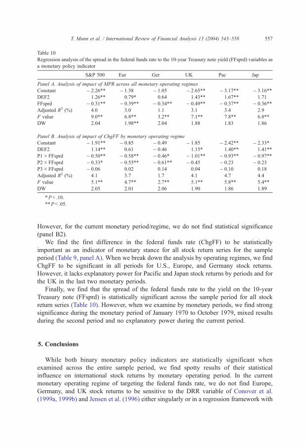
Table 10

Regression analysis of the spread in the federal funds rate to the 10-year Treasury note yield (FFsprd) variables as

a monetary policy indicator



Constant � 2.26** � 1.38 � 1.05 � 2.65** � 3.17** � 3.16**

DEF2 1.26** 0.79* 0.64 1.43** 1.67** 1.71

FFsprd � 0.31** � 0.39** � 0.34** � 0.49** � 0.37** � 0.36**

Adjusted R2 (%) 4.0 3.0 1.1 3.1 3.4 2.9

F value 9.0** 6.8** 3.2** 7.1** 7.8** 6.8**

DW 2.04 1.98** 2.04 1.88 1.83 1.86

Panel B. Analysis of impact of ChgFF by monetary operating regime

Constant � 1.91** � 0.85 � 0.49 � 1.85 � 2.42** � 2.33*

DEF2 1.14** 0.61 � 0.46 1.15* 1.40** 1.41**

P1� FFsprd � 0.50** � 0.58** � 0.46* � 1.01** � 0.93** � 0.97**

P2� FFsprd � 0.33* � 0.55** � 0.61** � 0.45 � 0.23 � 0.23

P3� FFsprd � 0.06 0.02 0.14 0.04 � 0.10 0.18

Adjusted R2 (%) 4.1 3.7 1.7 4.1 4.7 4.4

F value 5.1** 4.7** 2.7** 5.1** 5.8** 5.4**

DW 2.05 2.01 2.06 1.90 1.86 1.89

*P< .10.

**P< .05.


However, for the current monetary period/regime, we do not find statistical significance

(panel B2).

We find the first difference in the federal funds rate (ChgFF) to be statistically

important as an indicator of monetary stance for all stock return series for the sample

period (Table 9, panel A). When we break down the analysis by operating regimes, we find

ChgFF to be significant in all periods for U.S., Europe, and Germany stock returns.

However, it lacks explanatory power for Pacific and Japan stock returns by periods and for

the UK in the last two monetary periods.

Finally, we find that the spread of the federal funds rate to the yield on the 10-year

Treasury note (FFsprd) is statistically significant across the sample period for all stock

return series (Table 10). However, when we examine by monetary periods, we find strong

significance during the monetary period of January 1970 to October 1979, mixed results

during the second period and no explanatory power during the current period.

5. Conclusions

While both binary monetary policy indicators are statistically significant when

examined across the entire sample period, we find spotty results of their statistical

influence on international stock returns by monetary operating period. In the current

monetary operating regime of targeting the federal funds rate, we do not find Europe,

Germany, and UK stock returns to be sensitive to the DRR variable of Conover et al.

(1999a, 1999b) and Jensen et al. (1996) either singularly or in a regression framework with


an economic activity control variable. In the regression analysis, we find low statistical

sensitivity of U.S. stock returns to DRR and no indication of sensitivity when returns are

sorted into expansive and restrictive periods. We do find Pacific and Japan stock returns

strongly sensitive to DRR in the regression analysis. Most likely, this is due to the U.S.

being the largest trading partner of Japan. However, we are concerned about the efficacy of

DRR as a robust indicator of monetary policy to explain stock returns in all monetary

conditions and especially when the Fed uses a targeted federal funds rate.

We find that stock returns seem more sensitive to our hybrid MPR variable in the

regression studies especially during Period 3. This suggests possible use of the targeted

federal funds rate as an indicator of monetary stance in regression analysis in addition to

economic activity variables. We also find that monetary indicators based on the monthly

average federal funds rate produce spotty results by monetary operating periods. Perhaps,

the most consistent indicator to impact stock returns is the first difference in the federal

funds rate. Some of this result may be due to short-term frequency of the analysis.

We conclude that Fed operating procedures and/or target variables impact the

sensitivity of international stock returns to these five historical monetary policy indicators.

The results suggest caution in using any monetary policy variable to explain and possibly

forecast U.S. and international stock returns in all monetary conditions.

References

Bernanke, B., & Blinder, A. (1992). The federal funds rate and the channels of monetary transmission. American

Economic Review, 82, 901–921.

Brocato, J., & Steed, S. (1998). Optimal asset allocation over the business cycle. Financial Review, 33, 129–148.

Conover, C., Jensen, G., & Johnson, R. (1999a, July/August). Monetary conditions and international investing.

AAII Journal, 38–48.

Conover, C., Jensen, G., & Johnson, R. (1999b). Monetary environments and international stock returns. Journal

of Banking and Finance, 23, 1357–1381.

Fama, E. F. (1990). Stock returns, expected returns, and real activity. Journal of Finance, 45(4), 1089–1108.

Fama, E. F., & French, K. R. (1989). Business conditions and expected returns on stocks and bonds. Journal of

Financial Economics, 25, 23–49.

Jensen, G., Mercer, J., & Johnson, R. (1996). Business conditions, monetary operating regime and expected

security returns. Journal of Financial Economics, 40, 213–237.

Johnson, R., Beutow, G., & Jensen, G. (1999). International mutual fund returns and Federal Reserve policy.

Financial Services Review, 8, 199–210.

Meulendyke, A. (1998). U.S. monetary policy and financial markets. New York: Federal Reserve Bank of New

York.

Neal, C., Roley, V. V., & Sellon, G. H. (1998). Monetary policy actions, intervention and exchange rates: A

reexamination of the empirical relationships using federal funds rate target data. Journal of Business, 71,

147–177.

Ogden, J. (1990). Turn-of-month evaluations of liquid profits and stock returns: A common explanation for the

monthly and January effects. Journal of Finance, 45, 1259–1272.

Patelis, A. (1997). Stock return predictability and the role of the monetary sector. Journal of Finance, 52,

1951–1972.

Siegel, J. (1991). Does it pay stock investors to forecast the business cycle? Journal of Portfolio Manage-

ment, 28, 27–34.

Thorbecke, W. (1997). On stock market returns and monetary policy. Journal of Finance, 52, 635–654.

Documents

U.S. monetary policy indicators and international stock returns: 1970–2001