U.S. Economic Outlook 2Q2012

Economic OutlookUnited States

U.S. Economic Outlook

Index

1. Editorial ...................................................................................................................................................................................................................................................................... 1

2. Global Outlook ................................................................................................................................................................................................................................... 2

3. US Outlook ...................................................................................................................................................................................................................................................... 5

4. Regional Outlook: As the Winds Shift, Will the Service Sector Set Sail? ........................................................................ 9

5. Regional High-Tech Clusters Will Propel U.S. Growth.................................................................. 15

6. Assessing U.S. Potential Growth .......................................................................................................................................................... 21

7. How much growth of business loans should we expect .............................................. 25

8. Factsheet: A Focus on the U.S. Clean Economy .................................................................................... 29

9. Forecasts .......................................................................................................................................................................................................................................................... 30

See page 31 for the Disclaimer

Page 1


1. EditorialIn recent weeks, many analysts have raised concerns about the “fiscal cliff” that will hit the economy at the beginning of 2013. Under current legislation, the fiscal deficit will shrink significantly as a result of higher tax revenues and lower public spending. Estimates of this fiscal contraction fluctuate between 3.5% and 5% of GDP, which assuming standard fiscal multipliers, implies a considerable drag on GDP growth for next year. These worries are likely to increase as we move into the second half of 2012 and November’s Presidential elections.

The difference in these estimates reflects the way these figures have been calculated and the uncertainty that surrounds Congress’ actions with respect to the expiring provisions and the previously agreed spending cuts. First, these calculations incorporate different starting points and assumptions. If all provisions are combined, certainly the size of the contraction will be higher. However, some measures are likely to be extended, as they have been in the past, such as the alternative minimum tax patch and the “doc fix” (Medicare payments to physicians) that together add to more than $110bn. Other expiring tax provisions such as accelerated depreciation provide a relatively low bang for the buck and eliminating them will not have a significant impact on economic activity. These add up to another $20bn to $30bn. Allowing temporary extensions of unemployment benefits to expire may not have a large impact on economic activity if labor market conditions continue to improve, because these benefits would have been received by a lower amount of individuals anyway. Moreover, their reduction or elimination could also generate, at the margin, incentives to work. In a similar way, eliminating the payroll tax cut may not turn disastrous if in the aggregate, their benefits are partially offset by higher employment or if the multiplier effect is not as large as historical averages.

Other key considerations relate to the timing of the effects. Even if all the provisions of the 2001 and 2003 tax cuts were to expire, the drag would occur throughout 2013 and 2014 because part of the impact will occur when individuals complete their 2013 tax returns by April 2014. Second, and equally important, it is not clear that all provisions will expire as mandated by law, particularly the tax cuts for lower and middle income families. Judging by what leaders of both parties have stated on this issue, that assumption seems to be reasonable. In addition, Congress may choose to change or delay some of the previously agreed automatic spending cuts such as those for defense. The total magnitude of the drag from spending cuts could vary significantly if lawmakers focus on cutting spending with low fiscal multipliers.

Contrary to the direct effect of lower public spending, there could be large short-term positive effects from reducing the fiscal deficit if this is accompanied by eliminating the uncertainty that surrounds current fiscal policy. Furthermore, if many of these provisions end as planned or if public spending is reduced permanently, there could be added benefits from having a more certain fiscal environment. In fact, the current environment of low economic growth and large fiscal deficits suggests that we could already be experiencing negative effects from fiscal uncertainty. If economic agents perceive that large public spending and deficits imply higher taxes in the future or if short-term tax incentives generate large distortions to economic decisions, consumers and businesses are likely to down-shift their consumption and investment decisions to prepare for higher tax burdens in the future. Therefore, some degree of fiscal contraction could actually have positive effects if it is part of a more comprehensive strategy to eliminate tax distortions and provide a clear trajectory of fiscal sustainability.

Therefore, the debate among policy-makers has to shift from short-term fixes toward a grand bargain that assures fiscal sustainability over the long run. Whether this is done smoothly and over a few years it is not as important as implementing a credible and achievable strategy that tackles the most important fiscal challenges for the next decade. The pressures related to entitlement programs and tax policies are far larger and more relevant than immediate concerns, given that we are already on an unsustainable fiscal path. Delaying action, as has been the case in recent years, only imposes higher costs and burdens on future generations. Moreover, it places the economy at a higher risk if market expectations change suddenly. In this case it could prove too late to achieve a fix and regrets of wasted time will not provide solutions. Fortunately, there is time and plenty of options to move in the right direction if policymakers can pursue a bipartisan approach that puts economic efficiency at the top of the agenda.

Sincerely,

Nathaniel Karp

Page 2


2. Global Outlook

After a gradual deceleration during 2011, especially in the last quarter, the global economy is starting to pick up. We expect that global growth in 2012Q1 was higher than the previous quarter, given stronger growth in Asia ex China (including Japan), Latin America and sustained, but modest, dynamism in the US. We estimate that global growth will continue to increase and surpass 1% quarter-on-quarter at the end of 2012 (0.6% in 2011Q4). This recovery will also be quite heterogeneous, increasing the divergence of growth rates between the major world economies. The increase in growth in 2012 will be more evident in Asia due to the rebound of regional supply chains after natural disasters in Thailand and Japan and the partial reversal of the policy tightening measures implemented through mid-2011. Also, growth in Latin America is likely to pick up, as Brazilian growth rates increase on the back of easier monetary policy and Mexico maintains growth over 3.5% helped by US demand, improved competitiveness and supportive funding conditions. On the other hand, the US will continue sustaining quarterly growth rates of around 0.6% in 2012 and 2013, significantly lower than in previous recoveries. Still, this will be better than the basically stagnant activity in the euro-area in 2012. European growth will be dragged down by aggressive fiscal consolidation in peripheral countries and persistently high financial stress.

Therefore, emerging economies will recover their higher growth differential vis-à-vis developed economies of around 4 percentage points for 2012 and 2013. Concurrently, the growth gap between Europe and the US will also continue to widen during the next two years, even as we expect European authorities to continue taking decisive actions that will slowly lower financial tensions.

Overall, our growth projections are not very different from those of our previous Global Economic Outlook published in February. We expect global growth of 3.6% in 2012 and 4% in 2013, with emerging economies contributing around 80% of that increase in global activity (Chart 1). But, as mentioned before, this scenario is conditional on the evolution of the crisis in Europe and thus risks to these projections are still strongly tilted to the downside.

In this context, monetary policies in advanced economies will continue to be very accommodative for an extended period, fulfilling the role of bridging the slump in activity over the medium and long-run. However, while the effectiveness of further intervention is decreasing, the costs of additional measures increase, such as the risk of reduced central bank independence and the collateral damage from unconventional measures. Thus, other policymakers and institutions in the US and Europe must decisively engage and share the burden of reviving growth with central banks. They can implement economic and institutional reforms and manage fiscal risks. While these measures take effect, central banks should continue to support an adequate functioning of the monetary transmission mechanism.

Easy monetary policies in advanced economies mean favorable financing conditions in emerging countries. In these economies, central banks have to weigh the pressure from capital inflows and uncertain external demand against inflationary risks (in part from oil prices) and strengthening domestic demand. The difference in inflation projections in Asia and Latin America – declining in the former but stable in the latter – will condition a different outlook for monetary policies. We expect the easing cycle to have ended in much of emerging Asia (except in China and India), and a cautious tightening bias in most of Latin America apart from Brazil.

Page 3


In recent months, there have been some advances in solving the European crisis, but there are still many important pending issues. First, Greek sovereign debt held by the private sector was restructured, although substantial doubts about its long-run sustainability persist, including reform fatigue and a possible deeper recession than projected. Second, the European Stabilization mechanism (ESM) was provided with a fresh lending capacity of 500bn EUR (on top of 200bn already committed by the EFSF). However, that has not been enough to quell market anxiety, given that the total falls short of Spain and Italy’s financing needs for the next 3 years. Furthermore, the presumption that ESM loans would be senior to existing private bondholders seriously impairs its catalytic effect to attract further financing from the private sector. Compounding doubts, although the IMF increased its commitment by 430bn USD (approximately 330 bn EUR), it is not clear how much of that amount is targeted for European countries. Also, the fiscal compact was sanctioned (pending national approval), committing governments to structural deficits not bigger than 0.5% of GDP. This is a significant change towards controlling member’s budgets, but the allowance for deviations to the rule under “exceptional circumstances” may depict it as not strong enough to justify a more forceful action by hardliners at the ECB of core countries in Europe. In addition, there have been no advances towards a fiscal union or Eurobonds. In summary, a clear roadmap to where Europe is heading continues to be missing.

Chart 1 Chart 2

2.8

-0.6

5.1

3.9 3.6 4.0

-2

-1

0

1

2

3

4

5

6

2008 2009 2010 2011 (f) 2012 (f) 2013 (f)

Emerging Economies Adv. Economies

Baseline Feb-12 Baseline May-12

0

200

400

600

800

Oct11

Nov11

Dec11

Jan12

Feb12

Mar12

Apr12

May12

Ireland Spain Italy Belgium

France Netherlands Austria

Source: BBVA Research Source: Datastream and BBVA Research

Undoubtedly, one of the most important actions in the last four months was the provision of long-term liquidity by the ECB. This allowed, at least until March, a significant reduction in liquidity risk at European banks, a timid opening of wholesale funding markets and a compression of sovereign spreads in peripheral countries (Chart 2). But these positive effects proved temporary, as markets (i) detected some complacency on the part of policymakers as risk premia decreased in the first quarter of 2012, and (ii) they both doubted the ability of many peripheral countries to reach their fiscal targets and feared a fallout of growth if they actually achieved them. Thus, since March, risk premia increased rapidly in Italy and Spain, and in the latter, it rose to levels similar to the high tensions seen in November (Chart 2).

The short-lived effect of the long-term liquidity injections and the conundrum between fiscal consolidation and restoring growth highlight two conclusions. First, ECB actions can only bridge the short-run while the underlying economic and institutional problems are tackled. This means that talk of exit strategies for the ECB should not come too soon, but it also implies that economic reforms should be pushed forward, at the same time as demand is rebalanced within the Euro zone, with core countries stimulating it. Second, it is imperative to reconsider fiscal consolidation paths in a coordinated way (or risk being singled out by markets), targeting structural deficits –consistent with the spirit of the fiscal compact– in

Page 4


a more gradual trajectory. In exchange for more gradualism, member states must produce explicit, comprehensive, detailed and multi-annual consolidation plans. This way, sound public finances could be achieved without big damage to short-term growth. At the same time, this will allow Europe to reap the benefits of long-term structural reforms that are being implemented in peripheral countries.

In this context, we still see a new flare-up of the European crisis as the main risk, with potentially very negative consequences for global growth. Increased tensions can come about from reform fatigue in peripheral countries coupled with bailout fatigue in core countries, in the context of electoral processes in many European countries: France, Greece, Germany, Ireland and the Netherlands are holding either elections or a referendum in the first half of this year.

A second threat to the global economy is a further increase in oil prices. The recent spike at the beginning of 2012 can be traced back in part to tightening fundamentals (demand and supply) but also to an increase in the geopolitical risk premium to around 10-15 USD per barrel, given tensions around Iran and very reduced market buffers (oil inventories and producer’s spare capacity). In our baseline scenario, we consider prices around 120 USD per barrel of Brent oil for much of 2012, around 15% higher than in our February forecasts. In our view, this will only have a moderate negative impact on global growth, as central banks in advanced countries will view this as a temporary shock and their weak cyclical positions will prevent them from tightening monetary policy, one of the traditional channels of transmission to lower growth. Nevertheless, should the conflict in the Gulf escalate, there could be a very large spike in oil prices, and even if central banks still do not react, growth could be damaged through the associated increase in global risk aversion. We consider that the probability of an escalation in the Gulf is relatively low, but rising tensions could have a significant impact on global growth.

Page 5


3. US Outlook

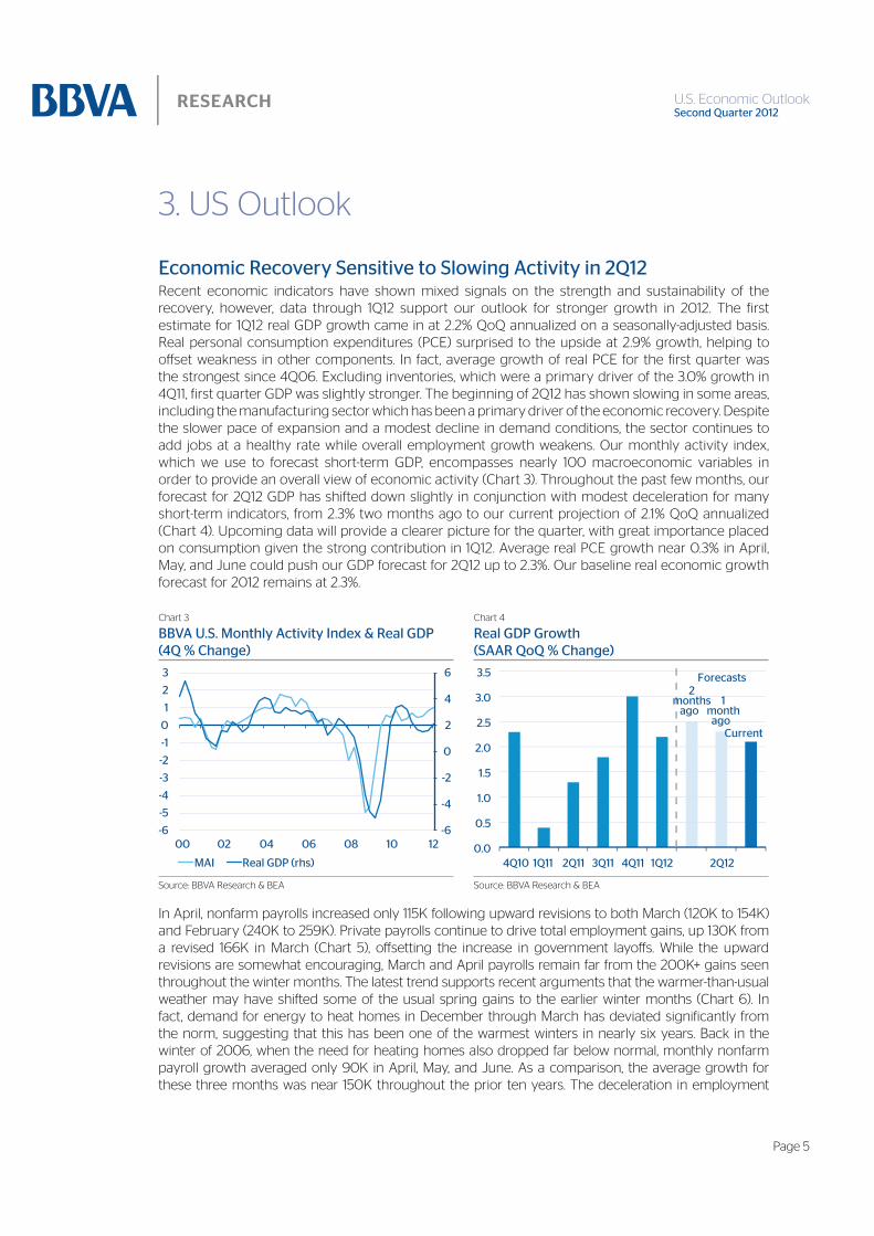
Recent economic indicators have shown mixed signals on the strength and sustainability of the recovery, however, data through 1Q12 support our outlook for stronger growth in 2012. The first estimate for 1Q12 real GDP growth came in at 2.2% QoQ annualized on a seasonally-adjusted basis. Real personal consumption expenditures (PCE) surprised to the upside at 2.9% growth, helping to offset weakness in other components. In fact, average growth of real PCE for the first quarter was the strongest since 4Q06. Excluding inventories, which were a primary driver of the 3.0% growth in 4Q11, first quarter GDP was slightly stronger. The beginning of 2Q12 has shown slowing in some areas, including the manufacturing sector which has been a primary driver of the economic recovery. Despite the slower pace of expansion and a modest decline in demand conditions, the sector continues to add jobs at a healthy rate while overall employment growth weakens. Our monthly activity index, which we use to forecast short-term GDP, encompasses nearly 100 macroeconomic variables in order to provide an overall view of economic activity (Chart 3). Throughout the past few months, our forecast for 2Q12 GDP has shifted down slightly in conjunction with modest deceleration for many short-term indicators, from 2.3% two months ago to our current projection of 2.1% QoQ annualized (Chart 4). Upcoming data will provide a clearer picture for the quarter, with great importance placed on consumption given the strong contribution in 1Q12. Average real PCE growth near 0.3% in April, May, and June could push our GDP forecast for 2Q12 up to 2.3%. Our baseline real economic growth forecast for 2012 remains at 2.3%.

Chart 3 Chart 4

-6

-4

-2

0

2

4

6

-6

-5

-4

-3

-2

-1

0

1

2

3

00 02 04 06 08 10 12

MAI Real GDP (rhs) 0.0

0.5

1.0

1.5

2.0

2.5

3.0

3.5

4Q10 1Q11 2Q11 3Q11 4Q11 1Q12 2Q12

Forecasts

Current

2months

ago 1

monthago

Source: BBVA Research & BEA Source: BBVA Research & BEA

In April, nonfarm payrolls increased only 115K following upward revisions to both March (120K to 154K) and February (240K to 259K). Private payrolls continue to drive total employment gains, up 130K from a revised 166K in March (Chart 5), offsetting the increase in government layoffs. While the upward revisions are somewhat encouraging, March and April payrolls remain far from the 200K+ gains seen throughout the winter months. The latest trend supports recent arguments that the warmer-than-usual weather may have shifted some of the usual spring gains to the earlier winter months (Chart 6). In fact, demand for energy to heat homes in December through March has deviated significantly from the norm, suggesting that this has been one of the warmest winters in nearly six years. Back in the winter of 2006, when the need for heating homes also dropped far below normal, monthly nonfarm payroll growth averaged only 90K in April, May, and June. As a comparison, the average growth for these three months was near 150K throughout the prior ten years. The deceleration in employment

Page 6


growth in March and April 2012 suggest that we are likely to see a similar impact throughout the rest of 2Q12. Given the latest trends in initial jobless claims, we expect that nonfarm payroll growth will remain below 200K on average at least for the short-term. Federal Reserve Chairman Bernanke has emphasized this weakness in his recent speeches, noting that current labor market trends imply around 150K to 200K in job creation per month to reduce the unemployment rate. A job creation pace of 100K, according to Bernanke, would keep the unemployment rate stable. As it stands now, businesses are not yet comfortable enough with demand conditions to expand their production levels, though we surmise that some have hired new workers simply because they have maximized their productivity with their current employee base. The unemployment rate surprisingly declined to 8.1% in April but once again reflected a decline in the labor force. The participation rate dropped to 63.6%, the lowest since December 1981, highlighting the potential for an increasing unemployment rate if more individuals enter (or re-enter) the workforce.Chart 5 Chart 6

-1000

-800

-600

-400

-200

0

200

400

07 08 09 10 11 12

Temporary Private ex C+M+TH

Construction+Manufacturing

0

100

200

300

0.95

0.96

0.97

0.98

0.99

1.00

1.01

1.02

Feb Apr Jun Aug Oct Dec

1994-07 2008-11 2012 job growth (rhs)


Recent increases in commodity prices persuaded the Federal Reserve to increase their outlook for inflation, but over the year they expect it to reside at or below their long-run target. In general, rising inflation has limited the Fed’s efforts to support the economy. However, unseasonably warm weather and the decline in natural gas prices appear to have limited the impact of high oil prices on headline inflation. Medical care and shelter prices have put upward pressure on core consumer prices (Chart 7), yet current trends do not pose significant risk to the Fed’s inflation goal. Inflation is expected to remain under control given the large output gap and stable inflationary expectations. Employment costs continue to increase, but growth rates remain low compared to historical trends. Alternative measures of underlying inflation, such as the trimmed-mean CPI and the median CPI, have decelerated on a YoY basis. Core PCE inflation, which the Fed follows closely, hovers just slightly below the 2% annual growth target (Chart 8). Looking forward, the distribution of prices in the consumer price index (CPI) suggests a decreasing central tendency. For 2012, our baseline scenario assumes 2.5% headline CPI. We have not revised our core inflation forecast and it remains at 1.9% for the year, although with some upside risk.

Despite prolonged weakness in the housing market, the latest data hint at some positive momentum and offer an improving outlook for the sector. Record affordability is helping to boost new home sales on a non-seasonally adjusted basis, and homebuilder confidence is improving. Inventories of new and existing homes for sale are declining and moving toward equilibrium. Low inventories of new homes will continue to stimulate new construction as demand improves, suggesting that new residential construction projects will make a positive contribution to economic growth this year. While the floor in sales and housing starts appears to have been reached in 2011, national price indexes will see further declines in 2012 due to the overhang of foreclosed properties and the inventory of existing homes. Headline price declines are driven by the elevated percentage of distressed sales in the existing home market, and thus as the percentage of non-distressed sales rises, these declines will ease. Potential sellers are beginning to perceive greater demand and an improved selling environment, as median sales prices for new and existing homes are currently up on a year-over-year basis.

Page 7


Chart 7 Chart 8

-1

0

1

2

3

4

5

6

7

06 08 10 12

Services Less Energy

Shelter Medical Care

Transportation

-6

-4

-2

0

2

4

6

8

10

07 08 09 10 11 12

PCE Durable Goods

Nondurable Goods Services

Core PCE Target


Curtailing the flow of foreclosures is a key target of policymakers. The federal government is focused on aiding struggling homeowners, and borrower and lender incentives to refinance or modify mortgages are expected to increase. Government programs (i.e. HARP) and low mortgage rates are stimulating refinancing activity. A large-scale rental conversion program for real-estate owned properties could ease foreclosures, support home prices, and supply the rental market. The Treasury is expected to propose winding down Freddie Mac and Fannie Mae in the near term. The various options include a reduced government role, a government guarantee of private mortgages when markets are under severe stress, and government insurance for certain mortgages that are already guaranteed by private insurers. All three options would lead to higher costs and mortgage interest rates for borrowers. Given that President Obama supports government involvement, the last option is more probable. We do not expect that mortgage finance reform will be enacted in 2012 given the proximity to the presidential election. The uncertainty about the future of the mortgage finance system ultimately has negative effects on the housing market.

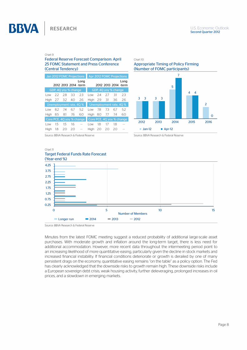
After the latest FOMC meeting, the Fed announced that it will continue to implement Operation Twist (lengthening the average maturity of its holdings of securities) and maintain its existing policy of reinvesting principal. The release indicates that members upgraded their economic outlook for 2012 compared to their forecast in January, but downgraded the 2013 and 2014 GDP forecasts (Chart 9). Given ongoing risks to the outlook (i.e. European sovereign debt issues) and persistent drags on growth (i.e. US fiscal consolidation and a depressed housing sector), conditions still “warrant exceptionally low levels for the federal funds rate at least through late 2014.” In response to a question during the press conference, Chairman Bernanke stated that in his personal view, the “exceptionally low levels for the federal funds rate” means a 0-0.25% Fed Funds rate; however, he stressed that individual FOMC members might have a differing view. Addressing the issue of quantitative easing, Bernanke’s opinion is that current conditions do not require any additional accommodative monetary policies. Furthermore, Bernanke and several FOMC members believe that the stock of assets is more important than the flow of assets in determining the interest rates. Therefore, we expect that Operation Twist will end as scheduled in June and the impact on the yield curve will be limited. Our expectation remains unchanged for a first Fed Funds rate increase in October 2014.

The fiscal outlook is warranting more attention as we get closer to the 2013 target. The Fed has become more vocal regarding the uncertain fiscal outlook, stressing the need for reforms and risks stemming from the expirations of several fiscal stimulus packages including the Bust tax-cuts. Bernanke believes that Congress should balance the two goals of fiscal sustainability and economic growth and asks for less austerity measures in the short term to sustain the economic recovery.

Page 8


Chart 9

Chart 10

3 3

5

4

2

3 3

7

4

0

2012 2013 2014 2015 2016

Jan-12 Apr-12

Source: BBVA Research & Federal Reserve Source: BBVA Research & Federal Reserve

Chart 11

0 5 10 15

0.25

0.75

1.25

1.75

2.25

2.75

3.75

4.25

Number of Members

2012 2013 2014 Longer run

Source: BBVA Research & Federal Reserve

Minutes from the latest FOMC meeting suggest a reduced probability of additional large-scale asset purchases. With moderate growth and inflation around the long-term target, there is less need for additional accommodation. However, more recent data throughout the intermeeting period point to an increasing likelihood of more quantitative easing, particularly given the decline in stock markets and increased financial instability. If financial conditions deteriorate or growth is derailed by one of many persistent drags on the economy, quantitative easing remains “on the table” as a policy option. The Fed has clearly acknowledged that the downside risks to growth remain high. These downside risks include a European sovereign debt crisis, weak housing activity, further deleveraging, prolonged increases in oil prices, and a slowdown in emerging markets.

Low 2.2 2.8 3.3 2.3 Low 2.4 2.7 3.1 2.3

High 2.7 3.2 4.0 2.6 High 2.9 3.1 3.6 2.6

Low 8.2 7.4 6.7 5.2 Low 7.8 7.3 6.7 5.2

High 8.5 8.1 7.6 6.0 High 8.0 7.7 7.4 6.0

Low 1.5 1.5 1.6 --- Low 1.8 1.7 1.8 ---

High 1.8 2.0 2.0 --- High 2.0 2.0 2.0 ---

Page 9


Chart 12

-6.00 to -1.44

-1.44 to -0.22

-0.22 to 0.82

0.82 to 2.37

2.37 to 9.49

Source: BBVA Research

4. Regional Outlook: As the Winds Shift, Will the Service Sector Set Sail?U.S. Industrial Production surged during the recovery: the year-over-year change peaked at 8.1% in June 2011 and has averaged 5.1% over the 24-month period from March 2010 to March 2012. This expansion is notable, as the pace is nearly 3 percentage points higher than the average pre-recession pace during 2002-2007. From 2008-2010, as the U.S. and European economies reeled during the aftermath of an over-expansion of credit, many developing economies continued to expand rapidly – in some cases, this growth was fueled by an expansion of domestic credit. Thus, as growth abroad proceeded, demand for U.S. exports surged ahead and created new manufacturing jobs throughout the U.S. Hard-hit manufacturing dependent cities in Indiana and Ohio greatly benefited from this resurgent demand. The strong growth in industrial production, however, slowed in early 2012, as the national index increased 0.7% during the first quarter. The pullback stemmed from several key industries, and reflects a changing pattern of growth generation throughout 2012.

In 2011, fervent international demand carried over into the oil, gas and coal mining sectors, as extraction activity drove industrial production last year. The rise in the price of oil and the ability to tap newfound shale reserves took hold in the energy sector, and energy-rich states such as Texas, North Dakota, Louisiana, Colorado, Wyoming expanded rapidly and created thousands of jobs. Furthermore, this growth seeped into other states such as Ohio and Pennsylvania whose energy potential was previously unknown. As energy exploration companies proceeded at full speed to extract as much natural gas and oil from shale as quickly as possible before leases expired, the price of natural gas steadily declined to bottom out around $1.83 per mmbtu in mid-April 2012.

The glut of natural gas and rock-bottom prices lowered the financial return of further drilling for natural gas, and thus exploration companies have stopped production at individual wells and shifted their resources to oil extraction. Through early May, the number of natural gas directed rigs is down 32% from May 2011. Consequently, production of dry shale gas declined sharply between February and April – most significantly in Texas’ Barnett and Haynesville shale plays and Pennsylvania’s Marcellus shale. This reduced production is resulting in rising prices: through mid-May, the price of natural gas has risen nearly 50 cents per mmbtu, and futures contracts anticipate a further rise. This slowdown in gas drilling activity is partly responsible for the moderation of industrial production in early 2012, as the oil and

Page 10


gas extraction component has declined in the first quarter. Going forward, we should expect further reductions in the number of gas drilling rigs as extraction companies pursue oil. Over the long term, however, the ample supply of gas is a massive opportunity for the United States; investments in new pipeline, processing and export infrastructure will drive growth as they are needed to fully harness this resource. Furthermore, elevated oil prices will continue to support investment in shale oil extraction through hydro-fracking techniques.

Another key driver of the recent slowdown in industrial production stems from the mining industry, as the production of coal and non-metallic minerals are each down over 15% in the first quarter. Although metal ore mining is up slightly during the first quarter, the dramatic falloff of the other two sectors reflects the weakening domestic and foreign demand. Here in the U.S., increasing environmental restrictions and cheap natural gas have caused many domestic electricity producers to shift their fuel from coal to natural gas. Further compounding this shift, the recent marked falloff in China and Brazil’s pace of activity has reduced the export market for both coal and non-metallic mineral products. Interestingly, in the U.S., the Wall Street Journal recently reported that the demand for Midwestern sand is skyrocketing due to its necessity in hydro-fracking. This activity along with iron ore mining should help to boost mining activity in the coming months, although the aggregate pace will be subdued over 2011’s double digit expansion.

Although mining and oil and gas extraction activities pulled back from last year’s pace, the outlook for overall industrial production remains positive as other industries are picking up some slack. First, the leading manufacturing industries include car and truck manufacturing along with engines and related equipment. Indeed, motor home manufacturing has led industrial production in early 2012 with a 25% expansion in the first quarter alone. Auto sales are steadily increasing over the previous year, and new auto inventories remain exceptionally low. Thus, with a leaner environment and improving sales, these sectors will continue to add to industrial output. A strengthening auto sector supports activity across a swath of related industries from synthetic fibers to audio equipment. Regionally, Michigan, many surrounding states, and Alabama all benefit from rising auto manufacturing activity.

Second, the nascent rebound in the housing market is also contributing to growth this year. For the first time since the recession, we expect residential investment to make a positive contribution to GDP this year. Indeed, in the first quarter of 2012, the winds have shifted for several industries related to the housing sector, as fabric and textile mills, household and institutional furniture, and paint manufacturing are all slightly positive. This turnaround is boosting output in North Carolina and in the southeastern U.S. The expansion of these manufacturing industries will continue alongside the uptick in residential investment as the paces of sales housing starts improve.

Chart 13

-5.00 to 0.04

0.04 to 0.54

0.54 to 0.88

0.88 to 1.33

1.33 to 4.57


Page 11


Looking across the U.S., we can see from Charts 1 and 2 how industrial production in MSAs with concentrations in mining and oil and gas has pulled back. For example, in 2011, Texas, Colorado, Louisiana and Wyoming had many dark blue areas that are now below the U.S. average. In Chart 3, West Virginia MSAs, Fairbanks, AK, Midland, TX, Duluth, MN, and Prescott, AZ lead the pullback section in 2012. Transportation manufacturing MSAs such as Kokomo, IN and Flint, MI lead the consistent expansion category while Mayaguez, Puerto Rico wins the title for best performance in early 2012 after a decline in 2011. Interestingly, many of the MSAs that saw a decline in industrial activity in 2011 are also among the weakest performers in 2012. These areas include, but are not limited to, Santa Fe, NM, Tallahassee, FL, Hinesville, GA, Dothan, AL and Atlantic City, NJ.

Moving forward in 2012, it is evident that a pullback in manufacturing and industrial production will require the service sector to strengthen and add workers to keep GDP growing. To date, the ISM non-manufacturing index has been consistently above 50, indicating that the service sector is expanding, and we believe that growth will continue. Nevertheless, the generation of jobs in the service sector relies on growing incomes and complementary output in production sectors. For example, on a year-over-year basis, the 11 states (or regions) with the highest private services growth are North Dakota, DC, Kentucky, Texas, Louisiana, Idaho, California, New York, Maryland, Colorado and Utah. Six of those states also benefited from a boom in energy-related production in 2011, while another three benefited from dollars flowing from the federal government, the technology sector propelled California and finance propelled New York. As the pace of private services job creation has also dwindled in recent data, we will increasingly be looking to these sectors for further signs of weakness and risks in the coming months.

Although more than 80% of all 370 MSAs registered a monthly contraction of industrial activity in recent data, the BBVA Compass Sunbelt’s industrial diversity has positioned it well in 2011, and it should be able to fend off a slowdown of national activity in 2012. Both on a year-over-year basis, and during the first quarter of 2012, the majority of the region’s MSAs display a positive growth differential with the U.S. average. This positive difference reflects the region’s leading manufacturing positions in transportation, technology, medical devices, machinery, metals and oil and gas exploration. For 2012, we expect the Sunbelt’s GDP to expand faster than the U.S. average due to these fundamentals that are responsible for above-average job creation and comparatively faster growth of population. The risk to California’s GDP growth, however, is tilted to the downside, as the state’s deteriorating fiscal situation will mandate higher taxes and further budget cuts this year. High unemployment and greater tax and regulatory burdens will further hamper growth. Meanwhile, Texas continues to attract people, companies, and technology workers as it diversifies its productive activity.

Chart 14

-2

-1.5

-1

-0.5

0

0.5

1

1.5

2

-0.2 -0.1 0 0.1 0.2 0.3 0.4 0.5 0.6 0.7 0.8 0.9 1 1.1

2011 Growth

Pullback in 2012 led bymining operations and oiland gas exploration

Positive Expansion

in 2012

2012

Gro

wth

Continuing Expansion Led by Auto Sector


Page 12


Chart 15

Anniston-Oxford, AL -0.19% 7.1% 3.3% 2.5% 1.8%

Auburn-Opelika, AL -0.14% 6.9% 3.1% 2.6% 1.9%

Birmingham-Hoover, AL -0.08% 2.3% -1.5% 0.3% -0.4%

Columbus, GA-AL -0.42% 4.3% 0.6% 1.7% 1.0%

Decatur, AL -0.32% 4.3% 0.5% 1.2% 0.5%

Dothan, AL 0.77% 0.5% -3.3% 1.0% 0.3%

Florence-Muscle Shoals, AL -0.84% 5.0% 1.3% 1.0% 0.3%

Gadsden, AL -0.24% 5.3% 1.6% 1.8% 1.1%

Huntsville, AL -0.14% 7.7% 3.9% 2.5% 1.9%

Mobile, AL -0.30% 5.5% 1.7% 1.4% 0.7%

Montgomery, AL -0.21% 6.6% 2.8% 2.5% 1.8%

Tuscaloosa, AL -0.82% 5.0% 1.3% -0.4% -1.0%

Flagstaff, AZ -0.30% 2.5% -1.3% 0.6% -0.1%

Phoenix-Mesa-Scottsdale, AZ -0.20% 5.2% 1.5% 1.3% 0.6%

Prescott, AZ -1.34% 2.0% -1.7% -2.3% -3.0%

Tucson, AZ -0.22% 2.9% -0.9% 0.1% -0.6%

Yuma, AZ -0.47% 3.8% 0.1% 1.2% 0.5%

Bakersfield, CA -0.02% 5.6% 1.8% -0.4% -1.1%

Chico, CA -0.18% 3.7% -0.1% 1.3% 0.6%

El Centro, CA -0.56% 2.1% -1.7% 0.7% 0.0%

Fresno, CA -0.08% 3.7% 0.0% 1.4% 0.7%

Hanford-Corcoran, CA -0.23% 2.8% -1.0% 1.2% 0.5%

Los Angeles-Long Beach-Santa Ana, CA -0.09% 5.1% 1.4% 1.8% 1.1%

Madera, CA -0.63% 4.5% 0.7% 1.7% 1.0%

Merced, CA -0.36% 2.7% -1.1% 1.2% 0.5%

Modesto, CA -0.29% 3.7% -0.1% 1.3% 0.6%

Napa, CA -0.36% 2.2% -1.6% 0.4% -0.3%

Oxnard-Thousand Oaks-Ventura, CA 0.09% 3.2% -0.5% 0.9% 0.2%

Redding, CA -0.51% 2.0% -1.7% 0.6% -0.1%

Riverside-San Bernardino-Ontario, CA -0.20% 4.0% 0.2% 1.5% 0.8%

Sacramento--Arden-Arcade--Roseville, CA -0.07% 4.5% 0.7% 1.4% 0.7%

Salinas, CA -0.15% 2.0% -1.8% 0.4% -0.3%

San Diego-Carlsbad-San Marcos, CA -0.08% 5.1% 1.3% 1.7% 1.0%

San Francisco-Oakland-Fremont, CA -0.20% 4.2% 0.4% 0.9% 0.2%

San Jose-Sunnyvale-Santa Clara, CA 0.00% 5.0% 1.3% 1.1% 0.5%

San Luis Obispo-Paso Robles, CA -0.30% 3.5% -0.2% 1.0% 0.3%

Santa Barbara-Santa Maria-Goleta, CA -0.18% 5.0% 1.2% 1.1% 0.4%

Continues on next page

Page 13


Santa Cruz-Watsonville, CA -0.07% 4.4% 0.6% 1.2% 0.5%

Santa Rosa-Petaluma, CA -0.10% 4.0% 0.2% 1.2% 0.5%

Stockton, CA -0.33% 4.0% 0.2% 1.5% 0.8%

Vallejo-Fairfield, CA -0.03% 3.2% -0.6% 1.2% 0.5%

Visalia-Porterville, CA -0.26% 2.7% -1.1% 1.0% 0.4%

Yuba City, CA -0.29% 4.3% 0.5% 1.1% 0.4%

Boulder, CO -0.01% 3.8% 0.0% 0.9% 0.3%

Colorado Springs, CO -0.22% 4.4% 0.6% 1.0% 0.3%

Denver-Aurora, CO 0.11% 4.8% 1.0% 0.4% -0.3%

Fort Collins-Loveland, CO -0.02% 4.5% 0.7% 1.1% 0.4%

Grand Junction, CO -0.13% 7.9% 4.2% 0.6% -0.1%

Greeley, CO 0.00% 5.9% 2.1% 0.6% -0.1%

Pueblo, CO -0.19% 4.2% 0.4% 1.3% 0.6%

Cape Coral-Fort Myers, FL 0.05% 2.4% -1.3% 1.2% 0.5%

Deltona-Daytona Beach-Ormond Beach, FL 0.06% 4.6% 0.8% 1.9% 1.2%

Fort Walton Beach-Crestview-Destin, FL -0.06% 8.9% 5.2% 3.1% 2.5%

Gainesville, FL -0.13% 3.6% -0.2% 1.6% 1.0%

Jacksonville, FL -0.19% 4.5% 0.7% 1.8% 1.1%

Lakeland, FL -0.24% 2.7% -1.1% 0.6% -0.1%

Miami-Fort Lauderdale-Miami Beach, FL -0.02% 3.6% -0.1% 1.5% 0.8%

Naples-Marco Island, FL -0.03% 4.2% 0.4% 2.0% 1.3%

Ocala, FL -0.16% 5.2% 1.5% 1.7% 1.0%

Orlando, FL -0.03% 5.7% 1.9% 2.2% 1.5%

Palm Bay-Melbourne-Titusville, FL 0.02% 5.8% 2.1% 1.6% 0.9%

Panama City-Lynn Haven, FL -0.40% 6.0% 2.2% 1.8% 1.2%

Pensacola-Ferry Pass-Brent, FL 0.16% 2.5% -1.3% 1.2% 0.5%

Port St. Lucie-Fort Pierce, FL 0.14% 4.8% 1.1% 2.0% 1.3%

Punta Gorda, FL -0.38% 2.1% -1.6% 0.5% -0.2%

Sarasota-Bradenton-Venice, FL 0.04% 4.3% 0.6% 1.7% 1.1%

Tallahassee, FL -0.24% 1.4% -2.3% 0.3% -0.4%

Tampa-St. Petersburg-Clearwater, FL -0.05% 4.1% 0.3% 1.5% 0.9%

Vero Beach, FL 0.01% 6.9% 3.1% 2.4% 1.8%

Albuquerque, NM -0.11% 4.2% 0.5% 1.1% 0.4%

Farmington, NM 0.04% 8.3% 4.5% 0.0% -0.7%

Las Cruces, NM -0.07% 4.3% 0.5% 1.4% 0.8%

Santa Fe, NM 0.18% 0.1% -3.7% -0.2% -0.9%

Continues on next page

Page 14


Abilene, TX 0.08% 5.5% 1.7% 0.5% -0.2%

Amarillo, TX -0.08% 5.0% 1.2% 1.4% 0.8%

Austin-Round Rock, TX -0.04% 4.5% 0.7% 0.8% 0.1%

Beaumont-Port Arthur, TX -0.18% 4.3% 0.5% 0.6% -0.1%

Brownsville-Harlingen, TX -0.18% 6.3% 2.5% 2.6% 1.9%

College Station-Bryan, TX -0.05% 5.8% 2.1% 0.7% 0.0%

Corpus Christi, TX -0.23% 6.4% 2.6% 0.1% -0.6%

Dallas-Fort Worth-Arlington, TX 0.04% 5.7% 2.0% 1.2% 0.5%

El Paso, TX -0.66% 4.3% 0.6% 1.3% 0.7%

Houston-Baytown-Sugar Land, TX 0.41% 5.6% 1.8% -0.1% -0.8%

Killeen-Temple-Fort Hood, TX -0.49% 3.6% -0.2% 1.0% 0.3%

Laredo, TX -0.01% 7.9% 4.1% 0.2% -0.5%

Longview, TX 0.14% 6.8% 3.0% 0.9% 0.3%

Lubbock, TX -0.06% 3.3% -0.5% 1.1% 0.4%

McAllen-Edinburg-Pharr, TX 0.01% 6.0% 2.3% 0.8% 0.1%

Midland, TX 0.35% 6.7% 2.9% -1.1% -1.8%

Odessa, TX 0.00% 8.8% 5.0% 0.8% 0.1%

San Angelo, TX 0.16% 4.8% 1.0% 1.0% 0.3%

San Antonio, TX -0.15% 5.7% 2.0% 1.5% 0.9%

Sherman-Denison, TX -0.02% 5.3% 1.5% 1.3% 0.6%

Tyler, TX 0.21% 6.4% 2.6% 0.8% 0.1%

Victoria, TX 0.16% 4.1% 0.3% 0.5% -0.2%

Waco, TX -0.10% 5.4% 1.7% 1.9% 1.3%

Wichita Falls, TX 0.02% 7.4% 3.7% 1.4% 0.8%


Page 15


5. Regional High-Tech Clusters Will Propel U.S. GrowthOver the past year, analysts, casual observers and journalists have questioned whether we are in “Tech Bubble 2.0,” as coined on the July 25, 2011 cover of Fortune magazine. During this time, the U.S. market has seen a doubling of Apple’s market value, a surge in the values of IBM and Google, a meteoric rise in the valuations of companies such as Zynga, Groupon, LinkedIn, and, as of press time, Facebook’s IPO that will value the social network at more than $100 billion. Critics contend that another bubble has been in the making and will burst as the market experienced in 1999-2000.

While the valuations of technology companies will be subject to volatility and may diverge from fundamentals, they are operating in a globally interconnected world and can now potentially reach billions of consumers simply by having a web presence. The proliferation of wireless networks and mobile devices has connected approximately 2.1 billion people to the Internet. Regardless of the euphoria surrounding Facebook’s massive valuation, consider that it claims to have nearly 500 million daily active users, and more than 901 million monthly active members – nearly three times the population of the United States. Their user base has nearly doubled in a scant two years. As investors continue to pour money into technology, the Facebook example underscores the new reality in which these companies operate, and the U.S. will continue to be a world leader in high-tech innovation.

The U.S. is the world’s innovation powerhouse and home of some of the most important technology clusters in the world. The U.S. leadership in technology and innovation has been possible due to the combination of several factors including a legal system that efficiently protects property rights, substantial public and private investments in research and development (R&D), the entrepreneurial spirit of the American society, an outstanding higher education system, a high-skilled workforce and the expertise built over several decades of innovation in science and engineering.

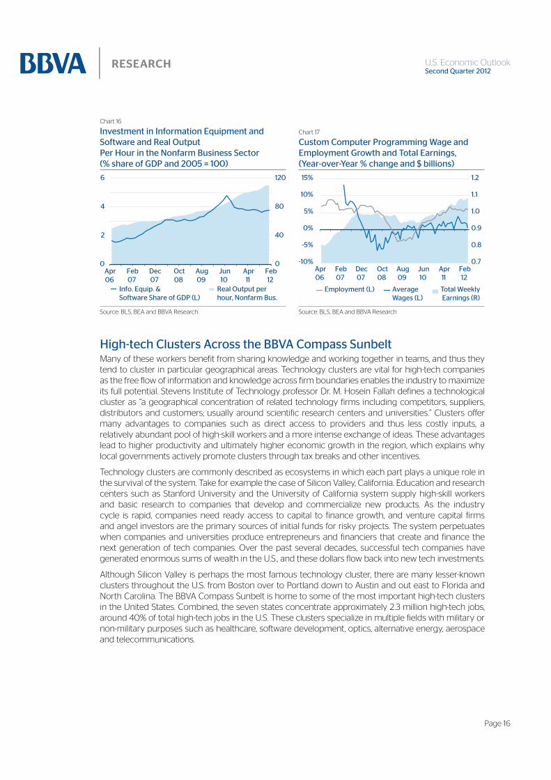
Researchers and innovators in the U.S. created the communication standards that allow the Internet to flourish, and U.S. academic institutions, engineers and computer scientists have an enormous stock of knowledge and experience to remain at the forefront of the high-tech industry. This long history of innovation and technology entrepreneurship continues to pay dividends to the U.S. economy. For example, the development and massive adoption of computers and networking technology during the 1990s resulted in higher output per worker and business productivity. Today, investment in Information Technology (IT) equipment and software is as vital as human capital. As a share of GDP, private investment in information processing equipment and software was 1.6% in 1970 and has averaged around 3.8% per year over the past decade.

Although many electronic components and computing devices are manufactured abroad, the innovation begins at home, and nearly 30% of total world exports of high-tech goods come from the United States. Job creation in the high-tech sector is occurring faster than average, and computer literate young people with programming and engineering skills are in high demand. More than 5 million people, approximately 4% of total non-farm payroll, work in the high-tech industry, and during the past twenty years, job creation averaged 1.3% annually versus 0.9% average of other industries. Some of the highest earning professions – no doubt due to their high educational attainment – are found in the high-tech industry. For example, in 2010, software programmers and computer and information research scientists earned median pay of $90,530 and $100,660, respectively - more than twice the median salary.

Page 16


Chart 16

Chart 17

0

40

80

120

0

2

4

6

Real Output per hour, Nonfarm Bus.

Info. Equip. & Software Share of GDP (L)

Apr06

Feb07

Dec07

Oct08

Aug09

Jun10

Apr11

Feb12

Total Weekly Earnings (R)

0.7

0.8

0.9

1.0

1.1

1.2

-10%

-5%

0%

5%

10%

15%

Apr06

Feb07

Dec07

Oct08

Aug09

Jun10

Apr11

Feb12

Average Wages (L)

Employment (L)

Source: BLS, BEA and BBVA Research Source: BLS, BEA and BBVA Research

Many of these workers benefit from sharing knowledge and working together in teams, and thus they tend to cluster in particular geographical areas. Technology clusters are vital for high-tech companies as the free flow of information and knowledge across firm boundaries enables the industry to maximize its full potential. Stevens Institute of Technology professor Dr. M. Hosein Fallah defines a technological cluster as “a geographical concentration of related technology firms including competitors, suppliers, distributors and customers; usually around scientific research centers and universities.” Clusters offer many advantages to companies such as direct access to providers and thus less costly inputs, a relatively abundant pool of high-skill workers and a more intense exchange of ideas. These advantages lead to higher productivity and ultimately higher economic growth in the region, which explains why local governments actively promote clusters through tax breaks and other incentives.

Technology clusters are commonly described as ecosystems in which each part plays a unique role in the survival of the system. Take for example the case of Silicon Valley, California. Education and research centers such as Stanford University and the University of California system supply high-skill workers and basic research to companies that develop and commercialize new products. As the industry cycle is rapid, companies need ready access to capital to finance growth, and venture capital firms and angel investors are the primary sources of initial funds for risky projects. The system perpetuates when companies and universities produce entrepreneurs and financiers that create and finance the next generation of tech companies. Over the past several decades, successful tech companies have generated enormous sums of wealth in the U.S., and these dollars flow back into new tech investments.

Although Silicon Valley is perhaps the most famous technology cluster, there are many lesser-known clusters throughout the U.S. from Boston over to Portland down to Austin and out east to Florida and North Carolina. The BBVA Compass Sunbelt is home to some of the most important high-tech clusters in the United States. Combined, the seven states concentrate approximately 2.3 million high-tech jobs, around 40% of total high-tech jobs in the U.S. These clusters specialize in multiple fields with military or non-military purposes such as healthcare, software development, optics, alternative energy, aerospace and telecommunications.

Page 17


Chart 18

0 to 4

4 to 8

8 to 36

36 to 953

No data


Chart 19

0 to 13

13 to 76

76 to 127

127 to 5167


The state is home to Cummings Research Park in Huntsville, a public-private partnership of businesses and government. The research park is the second largest research park in the United States with approximately 285 companies and 25,000 employees, and it specializes in more than 40 different technology fields. Military contracts support significant research and development, as some of the nation’s largest defense and aerospace firms reside here.

The engineering services industry is the largest employer in Arizona’s high-tech industry (17,650 in 2010). The biggest industries operating in the state are semiconductors and guided missile and space vehicle manufacturing. In addition, the Tucson Optics Cluster (TOC) is home to over 300 companies and organizations. Companies in the TOC specialize in biotech, defense, astronomy, aerospace, consumer electronics, display technology, data storage, healthcare, security, and telecommunications.

Page 18


Chart 20

0 to 22

22 to 101

101 to 434

434 to 7618

No data


Chart 21

0 to 5

5 to 18

18 to 88

88 to 1641

No data


According to the TechAmerica Foundation, California ranks No.1 in high-tech jobs with more than 930,000 employees and approximately 42,000 establishments. Approximately 30% of California’s exports are computer and electronic products. California is home to Silicon Valley, the most important technology hub in the world, and it is supported by the world-class education and research institutions of Stanford University, CALTECH and The University of California system.

As of 2010, Colorado has nearly 157,000 high-tech workers that take home a total of $14.2 billion annually, and TechAmerica ranks the total payroll 12th in the nation. Colorado ranks third in the number of tech jobs per 1,000 private sector workers. Approximately 50% of Colorado’s exports are high-tech products, and core industries are computer and electronics manufacturing, transportation equipment manufacturing software publishing, and engineering services. Nanotechnology, satellite imaging, and photonics are gaining momentum. Much of this tech presence is concentrated in the Denver and Boulder areas.

Page 19


Chart 22

0 to 5

5 to 18

18 to 88

88 to 1641

No data


Chart 23

0 to 3

3 to 9

9 to 23

23 to 5052

No data


The Florida high-tech corridor is a regional economic development initiative of the University of Central Florida, the University of South Florida and the University of Florida. It runs primarily along Interstate 4 between Orlando and Tampa, and is a partnership of more than 25 local and regional economic development organizations and 14 community colleges. Firms in the corridor focus on agritechnology, aviation and aerospace, digital media, financial services, IT, life sciences, microelectronics, medical technologies, nanotechnology, optics and photonics, and sustainable energy.

Texas has the second largest high-tech job concentration in the country (456,500 in 2010). The leading high-tech industries in Texas include computer, electronics and aerospace manufacturing, bioscience and medical technology, and IT and professional technical services. Austin has been coined “Silicon Hills” and is now home to 3800 technology companies and 91,000 employees. Currently, for example, Apple, Google and Facebook are all looking to hire workers in Austin. It is supported by the University of Texas, the third largest patent generator in the country. Although Austin is growing rapidly and visibly attracting many high-tech entrepreneurs and companies, the Dallas area has been coined “Silicon Prairie” because approximately 220,000 employees work high-tech related companies – more than Houston and Austin combined. Furthermore, in Houston, the medical center manages more than $1.2 billion in annual research expenditures and has 21,000 scientists, researchers, and other advanced degree professionals in the life sciences. Estimates peg the Texas Medical Center’s annual regional economic annual impact at more than $14 billion.

Page 20


Chart 24

0 to 6

6 to 20

20 to 42

42 to 1043

No data


New Mexico ranks 5th in the concentration of a high-tech workforce, as 83 per 1000 private sector workers are employed in the high-tech industry, according to TechAmerica. Much of the state’s technology related R&D is financed by the federal government. Core industries include semiconductors, R&D testing labs, and engineering services. The state is home of some of the most important R&D institutions such as the federal Los Alamos National Laboratory, Sandia National Laboratories and White Sands Missile Range. Air Force Bases support aerospace and technology firms.

From software development to alternative energy and medical devices, the U.S. high-tech industry will drive growth over the next decades. Regional technology clusters offer firms access to other related companies in a relatively small footprint, access to suppliers, a large pool of high-skill workers and access to leading institutions such as universities and government research centers. Each state in the BBVA Compass Sunbelt is home to an important technology cluster that supports local growth and innovation; however, significant federal and state budget deficits risk tax increases and budget cuts that may shift the regional patterns of the industry’s growth. For example, proposed federal defense and R&D budget cuts could impact research efforts in Alabama, New Mexico and San Antonio, and further cuts to the University of California system’s budget jeopardize its competitive position as a source of educated workers and innovation. Furthermore, rising local tax burdens decrease competitiveness and threaten to imperil entrepreneurship. Nevertheless, these clusters throughout the U.S. will reap the fruits of expected wealth generation as technology proliferates throughout the world.

Page 21


6. Assessing U.S. Potential Growth

The United States is struggling with fiscal and economic challenges that threaten its potential growth. To boost economic growth in the coming decades, the U.S. needs another sustained boom from technology and policymakers need to consider targeted structural reforms. Our estimates suggest that over the next decade, the U.S. economy will grow at a slower rate than its historical average as population growth slows and the labor force participation rate declines. In this article we investigate the estimation of potential growth of the U.S. economy.

The concept of potential growth has an important place in economic theory and monetary policy discussions. Potential gross domestic product (GDP) represents the level of output that an economy can produce without raising the rate of inflation. However, it should not be considered as a production possibility frontier that cannot be exceeded. Indeed, economic growth can exceed estimated potential, but this comes with a price: higher inflation. If actual output rises above its potential level, then, due to elevated resource utilization, inflationary pressures would rise. In other words, a growth rate above its potential will be short-lived and create additional problems like inflation and increased volatility in economic activity. On the other hand, if actual output falls below potential, then resources become idle and inflationary pressures will fall. Therefore, it is crucial for the monetary policy authority to know the rate of potential output growth to keep inflation under control.

Despite the importance of the issue, there is no unique way to measure it and attempting to do so presents some difficulties because potential output is unobservable. Thus, the estimates and their uncertainty vary depending on the chosen method.

Economists have devised several different approaches and techniques to measure potential output. We employed four of them to compare and thus have a more robust estimate of the level of US potential output. We employed a Hodrick-Prescott (HP) filter, Unobserved Component (UC) Model with Kalman filter, UC Model with an extended Kalman filter and a production function approach.

Following the methodology presented in Ozbek and Ozlale (2005), actual output can be decomposed into two components: trend and cycle,

Yt = T

t + C

t (1)

where Yt , T

t , C

t represent the real output, trend and cycle, respectively. Those familiar with the concept

could easily recognize Ct as output gap. Following the literature, we assume that C

t follows a second-order

autoregressive process with an error term that has zero mean and constant variance. Tt is assumed to

be random walk with drift indicating the shocks to trend or potential output are permanent. The model can be summarized as:

Ct = �

1, t C

t–1 + �

2, t C

t–2 + �

t� (2)

�1, t

= � 1, t–1

+ �� 1, t� (3)

�2, t

= � 2, t–1

+ �� 2, t� (4)

Tt = �

t + T

t–1 + �

t� (5)

� t = �

t, – 1 + �

a , t� (6)

where error terms �t, �

� 1, t, �

� 2, t and �

a , t are i.i.d. with zero mean and and constant variances. The model

above is referred to as an Unobservable Components (UC) model because it attempts to estimate unobservable variables such as potential output using information from observable variables such as real GDP. After writing the model in a state space form, the model can be estimated using a recursive algorithm called a Kalman filter which uses guesses for the unobserved variables to predict the observed variables and updates the guesses to minimize the prediction error.

Page 22


In the UC model, we used two different versions of the Kalman filter. First, we estimate the model with a standard Kalman filter in which the coefficients are constant over time. Second, we allow the autoregressive coefficients in the cycle model to vary over time and offer more flexibility to the model. Since the unobserved components and variable parameters have to be estimated simultaneously, a nonlinear estimation method has to be used. The latter method is also known as an extended Kalman filter.

In a third specification we use the Hodrick-Prescott (HP) filter which is a smoothing procedure that has become popular in economics because of its flexibility and ease of use. However, there are many shortcomings of the HP filter and therefore, economists find potential output estimates using HP filter disputable. Nevertheless, we used it as a benchmark to compare with more structural and complex models.

Chart 25 Chart 26

-6

-4

-2

0

2

4

6

8

10

12

48 53 59 65 70 76 82 87 93 99 04 10 16

Kalman GDP

-6

-4

-2

0

2

4

6

8

10

12

48 53 59 65 70 76 82 87 93 99 04 10 16

Extended Kalman GDP

Source: BBVA Research Source: BBVA Research

The last model is structural and uses economic theory to isolate the cyclical effects from actual output using a standard production function in economic theory. We assume that the U.S. production function is constant returns to scale and this method allows us to estimate the potential GDP and decompose potential growth into the contributions of labor (hours, natural rate of unemployment, and working age population), capital and technological progress (productivity). Technological progress is calculated as a residual in the model.

Page 23


All of these models (except the production function model) are estimated using quarterly data from 1947 to 2017. The production function model is estimated using annual data from 1967 to 2017. The data after 2012:Q1 come from our BBVA Research baseline scenario which assumes that the participation rate would start to increase in 2014 at a gradual rate. Unemployment is assumed to decline slowly and the population growth rate is projected to be lower than 1%. All data are publicly available at the Bureau of Economic Analysis (BEA) and the Bureau of Labor Statistics (BLS).

Chart 27 Chart 28

-6

-4

-2

0

2

4

6

8

10

12

48 53 59 65 70 76 82 87 93 99 04 10 16

HP GDP

-6

-4

-2

0

2

4

6

8

10

12

69 73 77 82 86 90 95 99 03 08 12 16

Production Function GDP


The estimation results indicate that HP and UC models with a standard Kalman filter produce similar potential growth estimates for the U.S. economy. Both models indicate that the US economy has potential growth of 2.4% in the next 6 years. Whereas an extended Kalman filter and production function approach measure the potential output as 2.2% and 2.1% in the next 6 years, respectively. As we move into 2015, potential growth rises to a range between 2.4 and 2.7%. The production function has the lowest potential growth estimate whereas the UC model with a standard Kalman filter has the highest prediction.

Chart 29

-1

0

1

2

3

4

80 84 88 92 96 00 04 08 12 16

Wap Tfp Participation rate Capital Hours NAIRU Potential GDP


Page 24


The results indicate that the 2008 financial crisis seriously affected the U.S. economy’s potential growth rate. A standard Kalman filter estimates almost 0% potential growth during the financial crisis which is certainly not usual for a developed country. The results from HP and the extended Kalman filter are more reasonable as the increase in productivity during the financial crisis should limit the decline in potential growth. The difference between the specifications of the standard and extended Kalman filters might take into account any structural changes in the economy, and therefore using an extended Kalman filter will capture any changes.

Aside from solely producing an estimate of potential growth, the production function approach provides more detail about the source of changes to the potential. The estimates suggest that a majority of potential growth comes from growth in the working age population (wap) and total factor productivity (TFP). In the near term, labor’s contribution to potential growth increases due to the elevated number of unemployed workers who will return to work as economic growth proceeds. Although our analysis suggests that potential growth is increasing as the economy revives from a financial crisis, in later years potential growth converges to a level below its historical average due to a decline in the labor force participation rate and lower population growth.

In summary, we showed that U.S. potential growth can be estimated but estimates vary depending on the assumptions of the procedure. However, our model results indicate that although the U.S. potential growth will rise in the near term, it will converge to a growth rate lower than its historical average. There might be many different explanations for low U.S. potential growth, but our analysis reinforces the need for policymakers to tackle structural challenges such as education, health care, immigration and tax policy so that today’s youth do not experience slower economic growth and mobility than their parents’ generations. Certainly, the U.S. should not take high economic growth for granted.

Acemoglu, Daron. “The World our Grandchildren Will Inherit: The Rights Revolution and Beyond.” NBER Working Paper No. 17994, (2012).

Ozbek and Ozlale. “Employing the estended Kalman filter in measuring the output gap.” Journal of Economic Dynamics and Control. (2005). Vol 29. Pages 1611-1622.

Page 25


7. How much growth of business loans should we expect?

Over the past six month, commercial and industrial (C&I) lending at commercial banks increased each month on average by $15bn. This is a strong pace of growth and it begs the question of how much C&I loan growth we can expect in the future. In this article, we review a number of different approaches to conceptualizing C&I loan growth, from the academic and complicated to simple ratios from historical analysis. Our sense is that much of the recent booming growth in C&I is the result of uncoiling of fears and the rapid recovery in activity following the end of the recession. We expect, however, that the growth rate of C&I lending will slow down over the next 12 months and move closer to our estimated long-run growth rate of 6% to 7% that is based on our baseline scenario of sluggish growth. Naturally, this outlook is contingent on intervening events not occurring: another financial crisis or a recessionary spiral. C&I lending, however, has benefited from a reduced risk premium, recovered durable goods orders and commercial banks’ fierce competition over clients. The contribution to C&I loan growth from nominal GDP growth, however, is expected to remain at historic lows, according to our calculations.

Some researchers in the past have used the degree of credit standard tightening (via the Senior Loan Officer Survey) as means of describing what happens in the economy following surges in loan growth or credit standards. These researchers placed real GDP, oil prices, the GDP deflator, commercial and industrial lending at commercial banks and the tightening stance of senior loan officers into the same vector autoregression (VAR) to identify the shocks of one variable on another. In theory, this small system of equations should tell us what the typical reaction of C&I loan growth will be to different shocks, be they from interest rates, macroeconomic variables or loan standards. Oil prices serve as a measure of commodity shocks. The GDP deflator is the standard measure of inflation in the economy.

Chart 30 Chart 31

00

02

04

06

08

10

12

14

54 62 70 78 86 94 02 10

-40

-20

0

20

40

60

80

100

92 96 00 04 08 12


The model’s impulse responses suggest that a shock to oil much like we had in 2011H1 would after four quarters have little effect on loans, but would reduce growth, increase inflation and tighten loan standards. This is somewhat reminiscent of what occurred over a four quarter period, since loan standards eventually tightened, but we did have intervening pressures from US fiscal negotiations and also European sovereign debt bailouts. Another interpretation of the shocks suggests a 1% increase in tightening results in a subsequent accumulated 0.1% reduction in loans 10 quarters in the future. This of course adds up considerably when you realize the net tightening stance increased from zero to 83

Page 26


between 2007Q1 and 2008Q4. The main insight of this framework, however, is that a sudden tightening of C&I standards imparts a significant, lasting effect on real GDP, which is what is often termed a “credit crunch” effect. The model describes many possible events between 2011Q1 and 2012Q1, but it is hard to disentangle the primary drivers. As such, we will turn to a more applied framework next.

Chart 32 Chart 33

1 3 5 7 9 11

0.00

-0.01

-0.02

-0.03

-0.04

-0.05

-0.06

0.000

-0.025

-0.050

-0.075

-0.100

-0.125

-0.150

-0.175

-0.200

-0.225

00..000000

--00..020255

--00..050500

--00..007755

--00.1.10000

--00.1.12525

--00.1.15050

--00.1.17755

--00..202000

-0-0.2.22525

1 3 5 7 9 11


Chart 34 Chart 35

1 3 5 7 9 11

4

2

0

-2

-41 3 5 7 9 11

0.225

0.200

0.175

0.150

0.125

0.100

0.075

0.050

0.025

0.000


One way to consider the future direction of C&I lending is to closely examine how this category of lending relates to economic indicators that we believe explain its growth. If we imagine that there is a long-term relationship between C&I lending, durable goods orders, GDP growth and the risk premium, we can calculate the contribution of each of these variables to business loan growth. The risk premium in this sense is the spread between the US 10-year Treasury and a BBB corporate bond. This spread is supposed to embody the amount of compensation investors are given for holding a riskier asset. This measure of the risk premium is a market-based measure of economic uncertainty, corporate default risk and instability all rolled into one indicator. Durable goods orders proxy as a measure of business investment, although it may not capture investments into softer items like software. Using statistical tests, we determine that all these variables are cointegrated and can therefore be said to have a long-term relationship. This long-term relationship is estimated by an error-correction model (ECM). This method gives us an estimate of the long-run equilibrium level of C&I loans and also the historical contribution attributable to each variable.

Page 27


First, our ECM specification generates an equation for the long-run equilibrium level of C&I loans. Loan growth can be either above or below this trend through time, but the model predicts the speed at which it returns to the trend. Naturally, it is possible for there to be structural breaks causing this trend line to be different than in previous history, but our past work does not suggest that this is the case for C&I loans. Another intuitive way of thinking about this is that while household balance sheets experienced a credit bubble and subsequent deleveraging, corporate balance sheets never experienced these effects. As the graph below suggests, there are times when C&I growth is above or below the growth rate of the equilibrium. In particular, we see in 2004-2008 how loans grew at a much higher rate than implied by the long-run level. This is somewhat the case in the most recent data, but both C&I lending and the equilibrium level recovered significantly since the end of the recession. This result suggests that the high growth rates we are currently seeing are temporary phenomena. We expect a return to trend YoY growth in C&I lending of around 6% to 7% YoY in our baseline scenario in the long run.

Chart 36

Chart 37

2011 2012 2013 2014

25%

20%

15%

10%

5%

0%

-5%-30%

-20%

-10%

0%

10%

20%

30%

92 96 00 04 08 12

C&I Loans YoY Equilibrium Level YoY


Our second view of influences on C&I lending is based on the historical contribution of each variable. Based on the simple model outlined above, we can decompose the historical data into a forecast and the accumulated effects of the residuals. All of our values are in nominal terms for consistency. As such, we can see the contribution from GDP dropping off considerably following the collapse of Lehman Brothers. Additionally, we can see that both the risk premium and durable goods orders declines became less of a drag on C&I lending after the end of the recession, although this occurred with considerable lag following the crisis. In the past 12 months an improved risk premium has contributed strongly to the growth in C&I lending, but this effect is tapering off the more the financial system stabilizes, European sovereign debt issues notwithstanding. As such, we can expect a more tempered growth rate of C&I lending based on the fact that the normally-strong effect from growth will not exist since we are in a slow recovery. We can also expect a more tempered pace of C&I lending given the “relief factor” of uncoiling risk premium and revived durable goods is abating as well. Some years into the future the financial system may regain its health to the point where now-shunned methods of financing return to compete with bank loans for customers, such as commercial paper. This represents a potential downside risk, although bank loans and market-based funding have historically coexisted peacefully, for the most part.

Page 28


Chart 38 Chart 39

0

1

2

3

4

5

6

7

63 69 75 81 87 93 99 05 11

-0.20

0.00

0.20

0.40

04 06 08 10 12

Autoregressive GDP

Risk Premium Durable Goods


While our applied framework above seems to fit with our presupposed influences on C&I credit, we can turn to some qualitative evidence stemming from the Federal Reserve’s Senior Loan Officer Survey. Looking at the four surveys of 2011, a clear theme emerges: banks began the year lending strongly to medium and large firms as a result of increased competition from both other banks and nonbanks. This is partly because at this point in time, the delinquency rate on C&I loans recovered faster than most other types of loans. While the charge-off rate on C&I loans recovered at roughly the same pace as other loans, it did not reach as high a level as other loans. Another theme from the surveys of 2011 is that a less uncertain economic outlook contributed strongly to new C&I business. Taking the entire picture into view, the survey suggest that business loan demand recovered from a shocked state. Banks competed strongly in this loan segment as it offered far better prospects than other segments. This is not necessarily the robust mix of conditions you would see in a more normal, stronger recovery. As such this qualitative evidence also confirms our sense of decelerating C&I growth in the future.

Historical experience suggests that precipitous drops in C&I lending follow precipitous drops in business activity. Much of the recent boom we are experiencing now can be related to an uncoiling of the damage from the crisis and a rebound in industrial activity. C&I growth has certainly been rapid over the past several months, but we are far from anything resembling a bubble and we are most likely gravitating towards a long-run growth rate over the next several months. If we consider that the average nominal YoY growth of GDP since 1980 is around 5.4% and C&I loans is around 5.7%, we might expect around 5% growth of C&I loans over the next few years given our current outlook of sluggish growth. However, some of that history includes some severe bank crises and heated competition from nonbanks. The ratio of C&I loan growth to nominal GDP growth until 1980 is larger than during the post-1980 period. A good rule of thumb might be to assume a 1.2 ratio of loan growth to nominal GDP growth, which confirms our long-run equilibrium calculation of 6% to 7%.

Page 29


8. FactsheetChart 40

1 Waste Management and Treatment 386,116 18 Solar Photovoltaic 24,152

2 Public Mass Transit 350,547 19 Green Chemical Products 22,622

3 Energy-saving Building Materials 161,896 20 Biofuels/Biomass 20,680

4 Professional Environmental Services 141,046 21 Energy-saving Consumer Products 19,210

5 Recycling and Reuse 129,252 22 Battery Technologies 16,129

6 Green Consumer Products 77,264 23 Smart Grid 15,987

7 Green Building Materials 76,577 24 Electric Vehicle Technologies 15,711

8 Nuclear Energy 74,749 25 Lighting 14,298

9 HVAC and Building Control Systems 73,600 26 Water Efficient Products 13,066

10 Recycled-Content Products 59,712 27 Pollution Reduction 9,986

11 Remediation 56,241 28 Fuel Cells 7,041

12 Green Architecture and Construction Services 56,190 29 Solar Thermal 5,379

13 Hydropower 55,467 30 Waste-to-Energy 3,320

14 Professional Energy Services 49,863 31 Geothermal 2,720

15 Appliances 36,608 32 Renewable Energy Services 1,981

16 Air and Water Purification Technologies 24,930 33 Carbon Storage and Management 391

17 Wind 24,294 34 Wave/Ocean Power 371

Source: Brookings-Battelle Clean Economy Database

Chart 41 Chart 42

0%

20%

40%

60%

80%

Scientists& Engineers

Green CollarOccupations

Low Wage/Low SkillOccupations

Share of all CleanEconomy Occupations

Share of all U.S.Occupations

1.4

2.4

4.8

2.7

0

2

4

6

Biosciences FossilFuels

Inf. Technolgy Producing

CleanEconomy

Mill

ion

s o

f Jo

bs

Source: Brookings-Battelle Clean Economy Database and U.S. Bureau of Labor Statistics Source: Biosciences: Battelle and Biotechnology Industry Organization, “State Bioscience Initiatives 2010” (2010);

Chart 43

New York-Northern New Jersey-Long Island, NY-NJ-PA 152,034 1.8

Los Angeles-Long Beach-Santa Ana, CA 89,592 1.7

Chicago-Joliet-Naperville, IL-IN-WI 79,388 1.8

Washington-Arlington-Alexandria, DC-VA-MD-WV 70,828 2.3

Philadelphia-Camden-Wilmington, PA-NJ-DE-MD 54,325 2.0

San Francisco-Oakland-Fremont, CA 51,811 2.7

Atlanta-Sandy Springs-Marietta, GA 43,060 1.9

Boston-Cambridge-Quincy, MA-NH 41,825 1.7

Houston-Sugar Land-Baytown, TX 39,986 1.6

Dallas-Fort Worth-Arlington, TX 38,562 1.3

Source: Brookings-Batelle Clean Economy Database and Moody’s Analytics

Page 30


9. Economic Forecasts (YoY % Change)

Chart 44

Real GDP 1.7 2.1 Real GDP

Nonfarm Employment 1.2 1.5 Nonfarm Employment -0.2 0.0

Nom. Personal Income 5.1 3.4 Real Personal Income 1.0

Home Price Index -3.9 Home Price Index -5.4

Home Sales 1.9

Real GDP Real GDP

Nonfarm Employment 1.0 1.7 Nonfarm Employment 1.0 1.1

Real Personal Income 2.8 Real Personal Income 2.9


Real GDP Real GDP




Real GDP Real GDP




Note: We have temporarily removed our forecasts of state existing home sales due to the NAR’s suspension of estimates as of 3Q11. Source: BBVA Research, BEA, BLS, NAR, Census Bureau and FHFA

Chart 45

U.S. AL AZ CA CO FL NM TX

GDP (2010 $ Billions) 14,527 173 254 1,901 258 748 80 1,207

Population (2011 Thousands) 311,592 4,803 6,483 37,692 5,117 19,058 2,082 25,675

Labor Force (Mar '12 Thousands) 154,707 2,142 3,009 18,488 2,735 9,282 934 12,540

NonFarm Payroll (Mar '12 Thousands) 132,707 1,870 2,449 14,237 2,291 7,329 805 10,742

Unemployment Rate (Mar '12) 8.2 7.3 8.6 11.0 7.8 9.0 7.2 7.0

Total Building Permits, (YTD Mar '12) 111,050 1,845 3,429 5,602 2,391 9,408 884 18,633

Change in Building Permits (YTD YoY (%)) 18.7 -6.2 42.1 10.3 33.9 29.9 22.4 20.0

Home Ownership Rate (Jan '12) 65.4 71.6 65.9 54.4 64.5 67.8 68.0 65.6

Housing Prices (4Q11 YoY Change (%)) -2.4 -1.4 -2.3 -4.6 -2.7 -2.8 -4.7 1.5

Exports of Goods (4Q11 $ Billions) 384.1 4.7 4.3 41.4 1.9 16.9 0.6 66.2

Change in Exports (4Q11 YoY Change (%)) 10.6 9.2 4.7 6.9 5.6 12.7 56.3 15.3

Source: BEA, BLS, Census, WiserTrade and FHFA


DISCLAIMER

Investors who have access to this document should be aware that the securities, instruments or investments to which it refers may not be appropriate for them due to their specific investment goals, financial positions or risk profiles, as these have not been taken into account to prepare this report.

The market prices of securities or instruments or the results of investments could fluctuate against the interests of investors. Investors should be aware that they could even face a loss of their investment. Transactions in futures, options and securities or high-yield securities can involve high risks and are not appropriate for every investor. Indeed, in the case of some investments, the potential losses may exceed the amount of initial investment and, in such circumstances, investors may be required to pay more money to support those losses. Thus, before undertaking any transaction with these instruments, investors should be aware of their operation, as well as the rights, liabilities and risks implied by the same and the underlying stocks. Investors should also be aware that secondary markets for the said instruments may be limited or even not exist.

“BBVA is subject to the BBVA Group Code of Conduct for Security Market Operations which, among other regulations, includes rules to prevent and avoid conflicts of interests with the ratings given, including information barriers. The BBVA Group Code of Conduct for Security Market Operations is available for reference at the following web site: www.bbva.com / Corporate Governance”.

BBVA, S.A. is a bank supervised by the Bank of Spain and by Spain’s Stock Exchange Commission (CNMV), registered with the Bank of Spain with number 0182.


Emerging Economies:

[email protected]

Cross-Country Emerging Markets Analysis

[email protected]

Mexico

[email protected]

Macro Analysis Mexico

[email protected]

Asia

[email protected]

Latam Coordination

[email protected]

Argentina

[email protected]

Chile

[email protected]

Colombia

[email protected]

Peru

[email protected]

Venezuela

[email protected]

Global Areas:

Financial Scenarios

[email protected]

Economic Scenarios

Innovation and Process

[email protected]

Developed Economies:

[email protected]

Spain

[email protected]

Europe

[email protected]

United States

[email protected]

Financial Systems & Regulation:

[email protected]

Financial Systems

[email protected]

Pensions

[email protected]

Regulation and Public Policy

[email protected]

Market & Client Strategy:

[email protected]

Global Equity

[email protected]

Global Credit

[email protected]

Global Interest Rates, FX and Commodities

[email protected]

Chief Economist

+1 713 881 0663 [email protected]

[email protected]

[email protected]

[email protected]

[email protected]

[email protected]

[email protected]

Art & Lay out:

Documents

U.S. Economic Outlook 2Q2012