U.S. Earthquake Frequency Estimation- Ratemaking for Unusual Events

Stuart B. Mathewson, FCAS, MAAA

133

U.S. Earthquake Frequency Estimation - Ratemaking for Unusual Events

By Stuart B. Mathewson, FCAS

Abstract

In our work on ratemaking, financial modeling, catastrophe modeling and planning, actuaries ohen must estimate the expected frequencies of unusual events. However, actual historical data for unusual events is too sparse to be very useful, so we must look to other sources for help. One example of these rare events is earthquakes. In recent years, the scientific community has performed significant research to better estimate the likehoods of earthquakes throughout the United States. Papers published by that community have presented much information that should be helpful in our quest to use earthquake frequencies in ratemaking, modeling and other actuarial work. This paper will present a basic discussion of scientific measures to estimate earthquake probabilities, a list of useful sources, and a discussion of several issues important to the understanding of earthquake ratemaking.

Introduction

Actuaries traditionally have had difficulty pricing coverages that have potential for

large severity, but that have low frequency. Often, the prices charged for these

coverages are determined by underwriting judgment and market forces, with little or

no actuarial involvement. The catastrophe portions of property coverages are an

obvious example of this situation. Among the insured catastrophe perils, earthquake

is probably the most difficult to price.

Historically, pricing for the catastrophe portion of property rates has involved

averaging losses over decades and large regions. However, changes in exposures

and insurance coverages during those decades make traditional actuarial methods

based on insurers’ loss data very uncertain. The introduction of computer simulation

models for estimating potential catastrophe losses now gives actuaries tools to help

estimate catastrophe rates. For instance, the California Earthquake Authority, which

writes a majority of the personal lines earthquake business in California, uses rates

that were based on loss costs from computer simulation modeling. This type of

134

model simulates losses from a large number of specific possible events. In order to

convert these losses to loss costs, models take these simulated losses and apply

frequency estimates to each event. These frequency estimates are critical, since any

inaccuracy in frequency translates directly into inaccuracy in the loss costs.

The severity portion of an earthquake model carries significant uncertainty, but the

frequency portion is probably more difficult to estimate accurately. There have been

few historical events that have caused appreciable damage, and even fewer

catastrophic earthquakes. Historical evidence is of limited use. Those responsible

for ratemaking utilizing computer model output may believe that they don’t need to

know specifics about earthquake frequency since the estimates are imbedded in the

models that they use. However, it is important to understand how frequencies are

estimated because they are so critical to the rate that is indicated by the model.

This paper will describe some basics of how scientists estimate earthquake

frequencies, where to look for frequency information and current issues on which

experts disagree. The uncertainty of these estimates and the effect on ultimate rates

will also be discussed.

Experts

If insurance loss data is confined to too short a time span to be useable, we need to

find information elsewhere. The experts in earthquake frequency are seismologists

and geologists. Seismologists study the historical earthquake records and the

geological records. Geologists study the earth’s crust to estimate how often the

earth will move in certain areas. It is important to realize that 150-200 years is very

short in the framework of geologic time. Thus, the geologic record of many

thousands of years becomes paramount in estimating earthquake recurrence times.

We can look to published papers in professional journals, government publications

and professional meeting presentations for the latest scientific research. Some of the

sources for U. S. seismic frequency estimates are the Seismological Society of

America (SSA), United States Geological Service (USGS), California Division of Mines

135

and Geology (CDMG), Southern California Earthquake Center (SCEC), American

Geophysical Union (AGU), and Earthquake Engineering Research Institute (EERI).

Sources for earthquake frequencies outside of California include state geological

surveys. Of course, universities provide much of the research underlying all the

estimates. These groups are constantly providing new information to better

understand the chance of earthquake occurrence.

Methods

Since estimating recurrence is so uncertain, scientists use a number of methods to

arrive at their estimates. They measure the seismic slip of the earth’s crust and the

amount that slip that will be accounted for by an earthquake. They use statistical

measures to extend the historical record to estimate likelihoods of very rare events.

And, they use paleoseismic research to discover evidence of old earthquakes.

Seismic Slip Analysis

The earth’s crust is comprised of tectonic plates that continually move with respect

to one another. Where the plates meet, this movement is evidenced as strain in the

crust. When the strain builds to a certain level, the crustal rock cannot hold it any

more and it moves - earthquake! The amount of displacement resulting from this

release of strain is known as seismic slip. Overall slip along a plate boundary can be

estimated fairly accurately by modern measurement methods, so this method is

useful for seismic areas at plate boundaries. Seismologists observe displacement of

the ground in actual events, and can then estimate return times that accommodate

the slip rate. The amount of slip is correlated to the amount of energy released by

the earthquake, which is measured by the magnitude of the event. There are several

types of magnitude definition, but for the purposes of this paper, we are using

Richter Magnitude when we use the term.

A simplified example shows how this works. The San Andreas Fault is the boundary

between the North American and Pacific plates in California. Along that fault, there is

approximately two inches of plate movement per year. In the 1906 earthquake, there

136

was up to 20 feet of displacement at various places along the fault. At two inches a

year, it would take 120 years to build up enough slip to move that 20 feet. Thus, if

Figure 1

the San Andreas were a simple system that accommodated all the plate movement,

the return time for this event could be estimated at about 120 years.

The real world, of course, is significantly more complex. Figure 1 shows the major

faults in the San Andreas system in California. The faults are not simple lines, but a

series of fractures, of which only a few are shown. There is significant work in

apportioning the overall slip of two inches a year to individual faults, each capable of

taking up some of the slip. For instance, in the above example, the San Andreas

actually only accommodates about half the plate movement. In addition, there is the

possibility of more than one fault segment breaking in the same event (“cascading

event”) and the fact that the release of strain in an event on one fault can change the

strain in nearby parallel faults.

137

Gutenberg-Richter Relationship

The rate of earthquake activity within a fairly large region can be estimated using a

statistical approach, wherein the historical record of earthquake magnitudes and

frequencies are fitted to a logarithmic equation. This equation is:

LogN=a-bM

In this equation, N is the number of earthquakes of magnitude equal or greater than

magnitude M during a certain time period, while a and b are determined by fitting the

equation to the historical record. Figure 2 shows an example of a curve for southern

California.

This equation is used to estimate the likelihood of various earthquake magnitudes for

an area, as well as to extend the historical record to magnitudes greater than

historically observed. The use of the Gutenberg-Richter relationship is one of the

areas of controversy among experts. The argument about the applicability of this

relationship versus using a “characteristic earthquake” will be discussed later.

Figure 2

Gutenberg-Richter Relationship Southern California 1850.1996

138

Paleoseismology

Since frequency of great earthquakes is often measured in terms of centuries and the

U.S. historical record is less than 200 years, scientists have had to go beyond the

record to discover how long the time is between the big shakes. Paleoseismology,

the science of identifying and dating past earthquakes by examining the geological

record, has proven to be very useful in extending our knowledge back from the

historical record. There have been significant paleoseismic studies in most U.S.

seismic areas, some of which are discussed below.

In one such study in Oregon, Nelson’ and Bradley of the USGS studied soils buried

beneath marshes. These soils show evidence of ground subsidence, much of which

has probably been caused by major earthquakes. For instance, the 1700 earthquake

discussed below probably caused significant subsidence. There have been 16

disturbances in the past 7,500 years, implying an average return time of about 500

years, assuming all the disturbances were caused by earthquakes. These, however,

were not evenly spaced over the 7,500 years.

Up the coast in Washington, a similar study of buried soils showed one very large

shallow earthquake about 1,000 years ago on a fault that runs directly beneath

Seattle. Shallow earthquakes, less than 10 miles or so below the surface, can cause

significant shaking, since there is less of the crust to absorb the energy released by

the quake than from a deeper event.

The above work in Oregon and Washington is very important, since the Pacific

Northwest has the chance for a great subduction earthquake. That is, an earthquake

where one fault pushes under another and which can generate earthquakes of 9.0

magnitude or greater. The Juan de Fuca plate moving eastward beneath the North

American plate along the coast of Oregon, Washington and a portion of British

Columbia would cause this earthquake. Native American lore in that area told of a

great earthquake about 300 years ago. An earthquake of that size and type would

have almost certainly caused a major tsunami (seismic sea wave) that would have

139

proceeded across the Pacific. Accordingly, Japanese records were searched and, as

expected, there was a record of a tsunami in January 1700. From those records,

scientists have calculated that a great subduction event happened off the Pacific

Northwest coast on January 27, 1700.

Juan de Fuca Plate

--- --- 116~

Figure 3

In the New Madrid seismic area of the Central U.S., there has been great concern

about a large earthquake. This area suffered a series of great earthquakes

(magnitudes over 8.0) in 1811-1812, but there is very little historically to help us

estimate the return time of such an event. To investigate the area,

paleoseismologists such as Buddy Schwieg16 of the USGS and Steve Wesnousky” of

140

Nevada-Reno have dug trenches in the affected areas. The walls of the trenches

were then studied to see evidence of past earthquakes.

In the 1811-12 earthquakes, there was significant liquefaction of the soil. This is a

condition where the earthquake mixes sandy soil and water to create a fluid soil.

This condition is often evidenced as sand blows, fluid sand shooting up to the

surface, looking like large anthills. In the trenches, there was evidence of sand blows

that have been carbon-dated at approximately 900 and 1300 A.D, with two others in

the past 2,000 years. This would imply a return time of about 500 years for events

large enough to cause sand blows. Some of these may not have been quite as large

as the 1811-12 events, although one may have been larger. Thus, scientists have

estimated that events of over 8.0 probably have return times of between 400 and

1,100 years. There are a couple of items that show the difficulty in this type of

estimation. First, studies of different fault segments show different areas of

liquefaction at different times. In addition, Schweig and others have shown evidence

of another earthquake between 1400 and 1600 A.D.

There has also been significant trenching activity in Southern California. One very

interesting finding arose after the magnitude 7.3 Landers earthquake of 1992, east of

San Bernadino, which was an event that ruptured multiple faults. Kerry Sieh’” of Cal

Tech, discovered through trenching that some of these faults had not broken for over

10,000 years, so, of course, would have no historical record.

Sieh also has done work in the southern San Andreas Fault system (Pallet Creek) that

shows an additional source of uncertainty in likelihood estimation. In that area he

showed ten precisely dated earthquakes over the past 2,000 years. However, they

were not evenly spaced over that time. There were four clusters of two or three

events each preceded by periods of dormancy that lasted two to three hundred

years. Each cluster happened within a one hundred-year period. Thus, the long-

term recurrence for these events is about 200 years, but the time between specific

events could be much lower. Similar studies have indicated that clustering has

occurred in other locations, and is common. Thus, even when scientists can identify

141

the average recurrence time of an earthquake on a fault segment, the actual time

between events can vary significantly.

These are samples of paleoseismic research that have provided very helpful

information. From this information, we have much better estimates of probabilities

of very large events than available from history, but we are also aware of the

difficulties involved in the process, and the uncertainties introduced in the frequency

estimates.

Sources of Frequency Information

There are several publicly available sources of frequency estimates. Of course, given

the seismicity of California, that area has received the majority of the attention.

U.S.G.S. Open-File Report 88-398j9

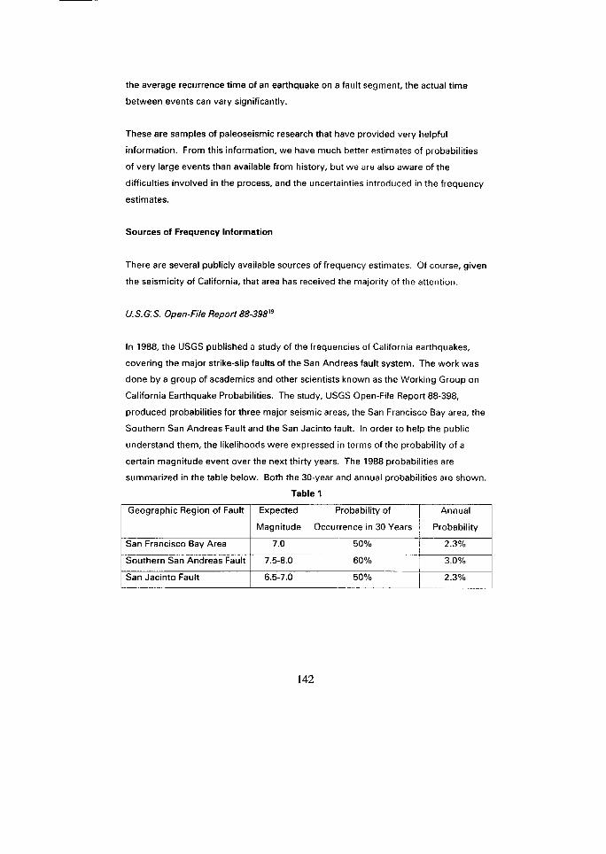
In 1988, the USGS published a study of the frequencies of California earthquakes,

covering the major strike-slip faults of the San Andreas fault system. The work was

done by a group of academics and other scientists known as the Working Group on

California Earthquake Probabilities. The study, USGS Open-File Report 88-398,

produced probabilities for three major seismic areas, the San Francisco Bay area, the

Southern San Andreas Fault and the San Jacinto fault. In order to help the public

understand them, the likelihoods were expressed in terms of the probability of a

certain magnitude event over the next thirty years. The 1988 probabilities are

summarized in the table below. Both the 30-year and annual probabilities are shown.

Table 1

142

U.S.G.S. Circular 1053”

The 1989 Loma Prieta earthquake on the San Andreas Fault south of San Francisco

precipitated a new look at the 1988 work. In 1990, the Working Group revised its

estimates for the San Francisco Bay Region, covering the North San Andreas Fault

and the Hayward Fault in the East Bay. This was published in USGS Circular 1053. In

addition to reflecting the change in stress after the Loma Prieta event, the Working

Group also considered faster fault-slip rate estimates and included the Rogers Creek

Fault, the northern extension of the Hayward Fault. The changes in probabilities are

shown in the following table.

Table 2

This is a rather significant increase over the 1988 estimate; even excluding the

Rodgers Creek Fault brings the 1990 estimate for the area to about 60%. a 20%

increase.

SCEC Study=’

The 1994 Northridge earthquake sparked another revision to the 1988 report, this

time for Southern California. The Southern California Earthquake Center coordinated

a new study by the Working Group that updated the Southern California probabilities

from the 1988 study (for the San Andreas and San Jacinto faults) and also

143

considered other potentially damaging earthquakes in that region. The study was

published in the April, 1995 issue of the Bulletin of the Seismological Society of

America (BSSA).

The modeling was considerably more complex and included the entire Southern

California region. The models predicted a 30-year probability for a magnitude 7 or

larger event of between 80% and 90%. Because of the differences in methodologies,

this study is hard to compare to the 1988 estimates, but it definitely increased the

perception of the earthquake problem in Southern California. The SCEC study added

several fault segments, included provision for “blind thrust-fault” earthquakes (those

that do not break the surface, for example, Northridge) and revised some slip rates

upwards. They also produced a method to include the chance of more than one fault

segment breaking in a single event (known as “cascading earthquakes”). The 1992

Landers and the 1857 Ft. Tejon earthquakes were examples of this type of event, so

this method should help provide more realistic estimates of return periods for large

events.

However, there has been some controversy about this study. When the predicted

probabilities are compared to the historical record, they exceed the historical

earthquake. The current discussions of that anomaly will be discussed later.

USGS Hazard Maps

In 1997, the USGS and the CDMG published new hazard maps for the U.S., showing

levels of ground shaking at specified exceedance probabilities throughout the

country. While these are not strictly frequency studies, these maps combine

frequency and severity, and as such, are good for comparing overall hazard to other

sources.

Non-California Sources

While this paper has concentrated on California probability sources, the potential loss

from earthquakes in other areas of the country is certainly important, and so are their

144

likelihoods. Other areas include the New Madrid seismic area, the Pacific Northwest,

Charleston, S. C., and Salt Lake City. Some sources for these areas, in addition to the

paleoseismic work above, are listed in the References section.

Ratemaking Effects

Loss costs underlying earthquake rates can be quite sensitive to the model frequency

estimates of the largest, most rare events. For instance, assume experts believe that

the return time for a magnitude 8 or greater event in the New Madrid seismic zone is

between 500 and 1,000 years. This size event would be considerably more

damaging than lesser events in a library of potential events in a model, so the choice

of frequency could have a significant effect on the total loss costs for that seismic

zone. As a simplistic example, see Table 3 on the next page. If the frequency of the

worst event in that table were doubled, the overall loss cost would rise from $7 to 10

million.

Current Controversies

Although seismologists have developed many very useful methodologies to improve

their earthquake probability estimates, there is still much uncertainty. There are

disagreements among the scientists about the best estimation methods. A few of

the current issues will be discussed to show the extent of the uncertainties.

Gutenberg-Richter vs. Characteristic Earthquakes

Earlier, the Gutenberg-Richter relationship was explained. While most will agree that

this is a useful concept, there is disagreement over when it should be used. For a

specific fault segment, many scientists believe that there will only be one certain size

event, known as a “characteristic” earthquake. They believe that strain will build to a

certain point, and then the fault will break. The amount of slip will be essentially the

same each time, and will result in a similar fault rupture and, thus, a similar

magnitude earthquake. For that fault, Gutenberg-Richter would not apply, since

there wouldn’t be a distribution of possible magnitudes. If this is true for all

145

individual fault segments, then Gutenberg-Richter is only a valid concept for a region

of such faults. The question is, “How big must a region be for the relationship to be

valid?”

This is a very important question for earthquake modeling, since assuming a

distribution of several possible magnitudes on a large number of faults may give

different answers than a distribution that assumes only one potential magnitude per

fault. It is typical for earthquake loss models to simulate several different magnitude

events on each fault segment, giving decreasing probabilities to increasing

magnitudes. If only one magnitude can happen, the distribution of probabilities by

magnitude for a library of events will be different.

In a simplistic case, we have assumed that the characteristic earthquake for a certain

fault is a 7.0, and a Guttenberg-Richter relationship shows the possibility of

damaging quakes from 6.0 to 7.5. We have also assumed that the losses for various

size events follow the pattern in the table below. The table shows potential losses

with assumed frequencies and losses for the spectrum of events where the total

annual frequency is 0.15 events per year.

Table 3

Magnitude

6.0

6.5

7.0

7.5

Annual Total

Annual Frequency

If the characteristic event of 7.0 were the only event to occur, the frequency of that

event would be 0.15. Thus, the annual average loss would be 0.15 x $100, or $15

million, more than twice that of the Gutenberg-Richter assumption. While this is a

simplistic example, differences like this can occur for a number of seismic areas, so

that this difference in opinion can potentially have a large overall effect.

146

The Paradox

In the August 1997 issue of the BSSA, Didier Sornette and Leon Knopoff14 published

a paper called, “The Paradox of the Expected Time until the Next Earthquake.” The

authors address the question; “Can it be that the longer it has been since the last

earthquake, the longer the expected time till the next?” This is in opposition to the

conventional wisdom says that, as the time since the last event increases, the

probability of the next occurrence increases. The common assumption is that strain

is released in an event, and then begins building up until it reaches a point that the

earth gives way again. This seems intuitively correct, but the authors argue that this

is not always the case. This is important for ratemaking, since the frequencies used

in the models often use the best estimate of the near-term frequency, rather than the

long-term frequency for an event. For example, if the long-term return time for a

certain earthquake is 100 years (frequency of 0.01). but it has been 75 years since the

last event of that type, the frequency used will be much higher than 0.01.

Their analysis suggests that the answer to this question depends on the inherent

statistical distributions of the fluctuations in the interval times between earthquakes.

Several distributions, including the periodic, uniform, semi-Gaussian and the Weibull

(with exponent greater than l), all have a decreasing return times with the passage of

time since the last event, as we would expect. However, the lognormal, power law

and Weibull with exponents less the 1 have increasing return times.

One explanation for this possibility is found in examining clusters of past

earthquakes. If we believe that earthquakes in an area behave in a clustering fashion,

we can expect a repeat of an event relatively shortly after an event that follows a long

dormancy. But, as the time following that event gets longer, we might believe that

we are in another long dormant time, rather than a time between clustered events.

In ratemaking, this means that the uncertainty of these events is increased. Not only

do we have to estimate the long-term frequency, with its uncertainty, but we also

have to factor in the effect of the time since the last event, and whether this increases

or decreases the frequency used in the ratemaking process for the next year.

147

The Enigma in the SCEC Report

As mentioned earlier, since the release of the SCEC report, seismologists have hotly

discussed the reasons why the estimates significantly exceed those implied by the

historical record. The graph in figure 4 shows the difference. The top line is the

predicted frequency, while the bottom is the historical record. Since this is a on

logarithmic scale, the prediction is actually about twice that of history in the

magnitude 6.0 to 7.0 range, where we find many damaging events.

Figure 4

Three possible reasons have been put forth to explain this difference. First, slip has

been taken up aseismically; that is, there has been slow movement of the earth

without earthquakes (“creep”) and folding of the crust. Secondly, we may have been

“lucky” over the past 150 years, or so. That is, the actual frequency has been

significantly lower than the long-term frequency for the area. Thirdly, there is the

possibility of an event much larger than the historical maximum, which was a Richter

magnitude of about 8.1. This may or may not be a significant problem, depending

on the accuracy of the historical record. That is, small changes in the magnitude

estimates of older historical events could account for much of the difference. The

report itself addressed this, suggesting that earthquake activity in the region for

magnitude 7 and greater earthquakes has be anomalously low since 1850, although

148

there was one great earthquake. Just one additional great earthquake would erase

the difference. This is one example of the sensitivity of earthquake frequency

estimates.

David Jackson of SCEC has been addressing this enigma with the following theory.

There seems to be no evidence that any significant creep has occurred in the area,

and, we can theorize that the 150-year period is long enough to show a reasonably

accurate estimate of long-term occurrence rates for medium earthquakes (magnitude

6-7), where the difference is greatest. Thus, Dr. Jackson has felt that the most likely

answer was that a much larger event could occur than the largest historical quake,

the 1857 Ft. Tejon event. This “mega-earthquake” needs only to have a return time

of about 1,000 years to take up the excess slip that is unaccounted for.

However, during the March 1998 annual meeting of the SSA, two teams of

researchers disputed the necessity for a “mega-earthquake.” SCEC has further

reviewed its study and found a number of small flaws that combined to overestimate

the estimate of the amount of slip building up in Southern California. They have

revised the model such that the difference between historical and theory has virtually

disappeared. At the same meeting, USGS scientists questioned the historical list of

magnitude 6 and greater events that was used by SCEC. They argue that the list may

have ignored quakes that occurred early in the time period, when inland California

was relatively unpopulated. They point out that the observed earthquake rate since

1903 is almost 50% greater than that recorded since 1850. If there were an

appropriately higher early rate, the SCEC difference would be reduced. This may or

not be the case, since 150 years of earthquake history is so short compared to

geologic time. (Note that the earthquake rate in the San Francisco area was very

high in the 70 years prior to 1906, and has been very low since.)

The answer to this enigma can certainly effect the loss costs that are modeled in

Southern California. If the “true” relationship includes about half the moderate

earthquakes that are currently reflected in a model, but has a very rare large one that

is not now reflected, “true” loss costs will certainly be different, although it is difficult

to estimate whether they would be higher or lower.

149

Conclusion

Now that scientifically based catastrophe modeling is being used to support

earthquake insurance rating, we must be aware of the importance of the probabilities

used and the uncertainty in those probabilities. The scientific community, led by the

USGS, CDMG and SCEC in California, continues to research the area to give us better

information. This research will continue to progress, and we can expect the

estimates to evolve. However, the significant disagreements among the scientists,

even in California, highlight the uncertainty involved.

We as ratemakers must be aware of the assumptions underlying the rates. When

loss costs are based on computer models, the frequency assumptions are often

buried in the models. We need to know the sensitivity of the estimates so we can

understand the uncertainty of the rates, and make informed pricing decisions.

150

References

1. Algermissen, S. T. et al, “Seismic Hazard Assessment in the Central and Eastern United States,” 1993 National Earthquake Conference, Monograph 1, Hazard Assessment, Central United States Earthquake Consortium, May 1994.

2. Bollinger, G. A., F. C. Davison and M. S. Sibol, “Magnitude Recurrence Relations for the Southeastern United States and its Subdivisions,” Journal of Geophysical Research, Vol. 94, No. 83, March 10, 1989.

3. Grant, L. B., J. T. Waggoner, T. K. Rockwell and C. von Stein, “Paleoseismicity of the North Branch of the Newport-lnglewood Fault Zone in Huntington Beach, California, from Cone Penetrometer Test Data,” BSSA, Vol. 87, No. 2, April 1997.

4. Hong, L.-L., and S.-W. Guo, “Nonstationary Poisson Model for Earthquake Occurrences,” BSSA, Vol. 85, No.3, June 1995.

5. Hopper, M. G., et al, “Estimation of Earthquake Effects Associated with Large Earthquakes in the New Madrid Seismic Zone,” USGS, Open-File Report 85-457, 1985.

6. Howell, B. F., “Patterns of Seismic Activity after Three Great Earthquakes in the Light of Reid’s Elastic Rebound Theory,” BSSA, Vol. 87, No.1, February 1997.

7. Nelson, A.R., et al, “A 7500-year Lake Record of Cascadia Tsunamis in Southern Coastal Oregon,” Geological Society of America Abstracts with Programs, V.28, 1996.

8. Nowroozi, A. A., “Seismotechtonic Map of the Southeastern United States,” Proceedings of the 1993 National Earthquake Conference, Central Untied States Earthquake Consortium, May 1994.

9. Nuttli, 0. W., “The Effects of Earthquakes in the Central United States,” Monograph Series Volume No. One, Central United States Earthquake Consortium, October, 1987.

10. Peterson, M. D. and S. G. Wesnousky, “Fault Slip Rates and Earthquake Histories for Active Faults in Southern California,” BSSA, Vol. 84, No. 5, October 1994.

11. Rizzo, P. C., N. R. Vaidya, E. Bazan, C. F. Heberling, “Earthquake Spectra, EERI, Vol. 11, No. 1, February, 1995.

12. Satake, K.. KShimazaki, Y. Ysuji, and K. Ueda, “Time and Size of a Giant Earthquake in Cascadia Inferred from Japanese Tsunami Records of January 1700,” Nature, v.379, 1996.

13. Sieh, K., L. Jones, E. Hauksson, et al, “Near-field investigations of the Landers Earthquake Sequence,” Science, April-July, 1992.

151

14. Sornette, D. and L. Knopoff. “The Paradox of the Expected Time until the Next Earthquake,” BSSA, Vol. 87, No. 4, August, 1997.

15. Thenhaus, P. C., D. M. Perkins, S. T. Algermissen, S. L. Hanson, “Hazard in the Eastern United States: Consequences of Alternative Seismic Source Zones,” Earthquake Spectra, EERI, Vol. 3, No. 2, May, 1987.

16. Tuttle, M.P. and ES. Schweig, “Archeological and Pedological Evidence for Large Prehistoric Earthquakes in the New Madrid Seismic Zone, Central United States,” Geology, v.23, 1995.

17. Wesnousky, S. and L. Leffler, “On a Search for Paleoliquifaction in the New Madrid Zone,” Seismological Research Letters, V.63, 1992.

18. Working Group on California Earthquake Probabilities, “Probabilities of Large Earthquakes in the San Francisco Bay Region, California,” USGS Circular 1053, 1990.

19. Working Group on California Earthquake Probabilities, “Probabilities of Large Earthquakes Occurring in California on the San Andreas Fault, USGS Open-File Report 88-398,1988.

20. Working Group on California Earthquake Probabilities, “Seismic Hazards in Southern California: Probable Earthquakes, 1994 to 2024,” BSSA, Vol. 85, No. 2, April 1995.

152