United States Drinking Water Quality Study Report

A Project Sponsored by the Procter & Gamble Company June 2006 – December 2006

Dr. Xinhao Wang, University of Cincinnati Charlotte White-Hull, the Procter & Gamble Company

Dr. Scott Dyer, the Procter & Gamble Company Diana Mitsova-Boneva, University of Cincinnati

Mayura Ghode, University of Cincinnati

March 13, 2007

2

1. Introduction

Community water systems regulated by Federal and State agencies serve ninety percent of the U.S. population (U.S. EPA, 2006). Source water for these systems includes groundwater, rivers, streams, springs, or lakes. Contamination of these raw water supplies may be naturally-occurring (e.g. erosion) or result from human influence (e.g. point and non-point pollution sources). In addition, occurrences such as pipe corrosion and disinfection may also result in contamination of drinking water provided to consumers. Contaminants may include microorganisms, inorganic and organic chemicals, and radioactive substances.

To address common contaminants and ensure the safety of community drinking water supplies, the U.S. Environmental Protection Agency and state agencies have established Drinking Water Standards (U.S. EPA, 2003). Although the treated water of United States generally meets these standards (U.S. EPA, 2006), water suppliers’ ability to meet them depends in part upon source water condition and infrastructure characteristics. Thus, a University of Cincinnati Drinking Water Quality Project was developed to provide information on the variability of drinking water quality for U.S. major metropolitan statistical areas. The project is comprised of a drinking water constituent database, developed as a Procter & Gamble-funded project in collaboration with University of Cincinnati, and a corresponding Web site.

The Project encompassed the seventy-seven most highly populated Metropolitan statistical areas(“MSAs”) of the contiguous United States, accounting for approximately sixty-two percent of the total U.S. population. For the study, drinking water contaminant data for representative water providers within each metropolitan statistical area were extracted from their annual Consumer Confidence Reports and captured in a Drinking Water Database. Twelve common contaminants reflecting water quality were selected for the study. Data sources used to develop the drinking water database include the United States Environmental Protection Agency, the U.S. Bureau of Census, and publicly available consumer confidence reports for the respective cities. Summary information from the database has been provided in a user-friendly format via a Drinking Water Quality Web site. The Web site consists of interactive maps and charts that display water quality data at the metropolitan statistical area and facility levels.

2. Data Collection Data collection consisted of three efforts: 1) selection of representative Metropolitan statistical areas; 2) selection of representative Drinking Water providers; and 3) collation of representative contaminant data.

Metropolitan Statistical Area (MSA) data were obtained from the U.S. Census Bureau (OMB, 2004). Due to resource limitations, not all metropolitan statistical areas could be included in the analysis. Therefore, the selection of metropolitan statistical areas aimed for a representative national spatial distribution, as well as incorporation of a majority of the urban population of the U.S. To accomplish this, eighteen Consolidated metropolitan statistical areas (CMSAs), or those having populations of one million or greater, were first selected. Next, the most-populated metropolitan statistical area from each state not falling within a CMSA boundary was selected, adding 30 MSAs. The 29 remaining MSAs having the highest population were then selected. Thus, a total of seventy-seven spatially-distributed metropolitan statistical areas, representing 577 counties and 62% of the population in the contiguous USA, were included in the final analysis (Figures 1-9).

To obtain representative water providers, a list of permitted providers for each MSA was first extracted from U.S. EPA’s Safe Drinking Water Information System (U.S. EPA, 2000). This system was created via implementation of the Safe Drinking Water Act and contains data describing U.S. public water systems. Water providers were selected from

3

this list in order of descending service population until the accumulative population was more than half of the MSA population. In cases where a drinking water supplier encompassed two or more water treatment plants, all of the water treatment plants for the supplier were incorporated into the data table. A total of 392 water utilities encompassing 705 treatment plants were included in the study.

Water quality contaminant data were obtained from each provider’s Consumer Confidence Reports (CCR) or Water Quality reports. Under the terms of U.S. EPA’s Safe Drinking Water Act, each community water system is required to supply an annual Consumer Confidence Report to its customers describing their drinking water source, any regulated contaminants detected in treated water, and compliance information. For this study, data was culled from the most recent report available online from a utility’s website. Thus, a mix of data from years 2004-2006 were included in the study.

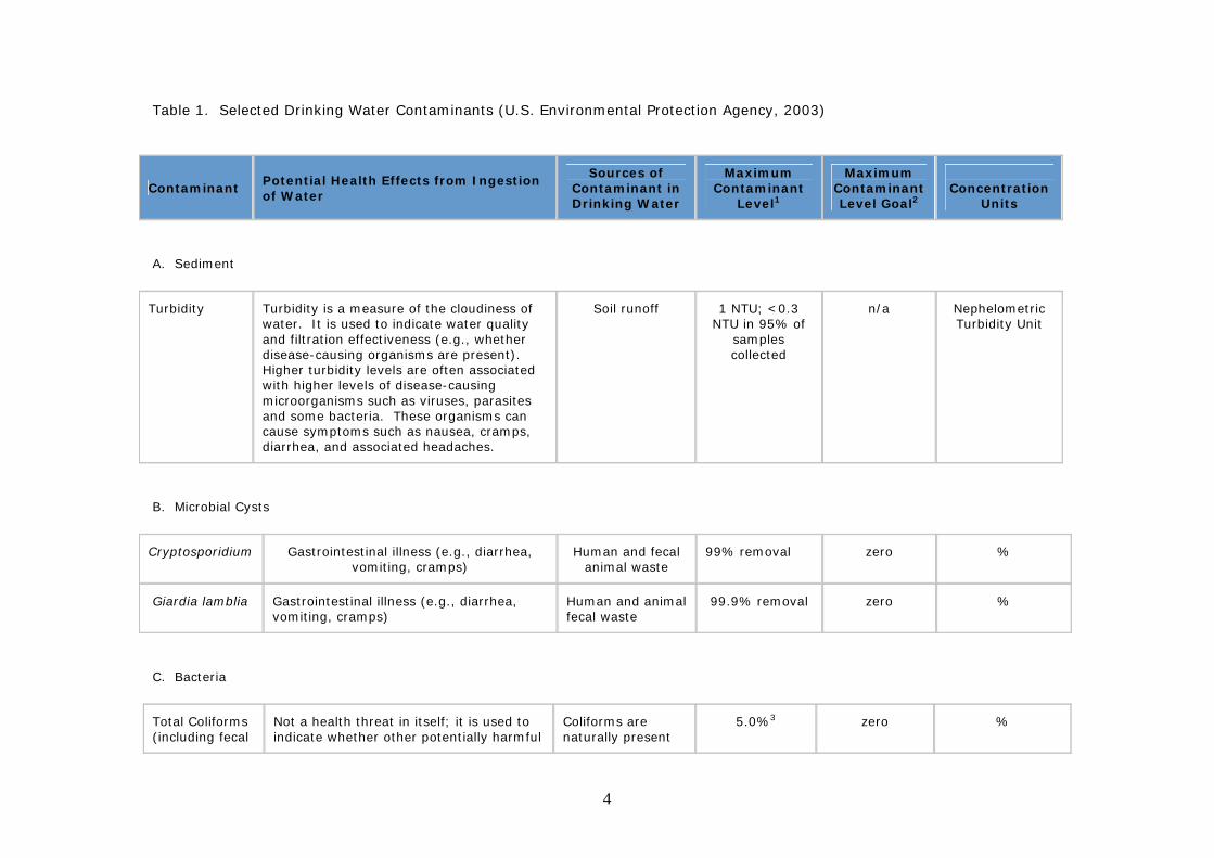
Twelve regulated and non-regulated contaminants were selected to summarize drinking water quality for the metropolitan statistical areas. The contaminants considered in this study were based on human safety considerations and data availability for the selected metropolitan statistical areas. Table 1 contains information potential contaminant sources, their health effects, as well as regulated permissible concentrations.

4

Table 1. Selected Drinking Water Contaminants (U.S. Environmental Protection Agency, 2003)

Contaminant Potential Health Effects from Ingestion of Water

Sources of Contaminant in Drinking Water

Maximum Contaminant

Level1

Maximum Contaminant Level Goal2

Concentration

Units

A. Sediment

Turbidity Turbidity is a measure of the cloudiness of water. It is used to indicate water quality and filtration effectiveness (e.g., whether disease-causing organisms are present). Higher turbidity levels are often associated with higher levels of disease-causing microorganisms such as viruses, parasites and some bacteria. These organisms can cause symptoms such as nausea, cramps, diarrhea, and associated headaches.

Soil runoff 1 NTU; <0.3 NTU in 95% of

samples collected

n/a Nephelometric Turbidity Unit

B. Microbial Cysts

Cryptosporidium Gastrointestinal illness (e.g., diarrhea, vomiting, cramps)

Human and fecal animal waste

99% removal zero %

Giardia lamblia Gastrointestinal illness (e.g., diarrhea, vomiting, cramps)

Human and animal fecal waste

99.9% removal zero %

C. Bacteria

Total Coliforms (including fecal

Not a health threat in itself; it is used to indicate whether other potentially harmful

Coliforms are naturally present

5.0%3 zero %

5

coliform and E. Coli)

bacteria may be present5 in the environment; as well as feces; fecal coliforms and E. coli only come from human and animal fecal waste.

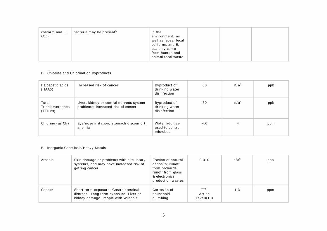
D. Chlorine and Chlorination Byproducts

Haloacetic acids (HAA5)

Increased risk of cancer Byproduct of drinking water disinfection

60 n/a4 ppb

Total Trihalomethanes (TTHMs)

Liver, kidney or central nervous system problems; increased risk of cancer

Byproduct of drinking water disinfection

80 n/a4 ppb

Chlorine (as Cl2) Eye/nose irritation; stomach discomfort, anemia

Water additive used to control microbes

4.0 4 ppm

E. Inorganic Chemicals/Heavy Metals

Arsenic Skin damage or problems with circulatory systems, and may have increased risk of getting cancer

Erosion of natural deposits; runoff from orchards, runoff from glass & electronics production wastes

0.010

n/a5 ppb

Copper Short term exposure: Gastrointestinal distress. Long term exposure: Liver or kidney damage. People with Wilson's

Corrosion of household plumbing

TT6; Action

Level=1.3

1.3 ppm

6

Disease should consult their personal doctor if the amount of copper in their water exceeds the action level

systems; erosion of natural deposits

Lead Infants and children: Delays in physical or mental development; children could show slight deficits in attention span and learning abilities. Adults: Kidney problems; high blood pressure

Corrosion of household plumbing systems; erosion of natural deposits

TT6; Action

Level=0.015

Zero ppm

Nitrate (measured as Nitrogen)

Infants below the age of six months who drink water containing nitrate in excess of the MCL could become seriously ill and, if untreated, may die. Symptoms include shortness of breath and blue-baby syndrome.

Runoff from fertilizer use; leaching from septic tanks, sewage; erosion of natural deposits

10 10 ppm

F. Taste/Odor

Taste/Odor Seasonal effects include musty, moldy, earthy, grassy or fishy taste/odor, a result of certain types of algae, fungi, and bacteria growing in the water supply, especially during warm weather. There are no potential health effects.

Several potential sources -abnormalities reported to or by water utilities

Taste and Odor characteristics are not regulated by

U.S. EPA

n/a n/a

1. Maximum Contaminant Level (MCL) - The highest level of a contaminant that is allowed in drinking water. MCLs are set as close to MCLGs as feasible using the best available treatment technology and taking cost into consideration. MCLs are enforceable standards. 2. Maximum Contaminant Level Goal (MCLG) - The level of a contaminant in drinking water below which there is no known or expected risk to health. MCLGs allow for a margin of safety and are non-enforceable public health goals. 3. More than 5.0% samples total coliform-positive in a month. (For water systems that collect fewer than 40 routine samples per month, no more than one sample can be total coliform-positive per month.) Every sample that has total coliform must be analyzed for either fecal coliforms or E. coli if two consecutive TC-positive samples, and one is also positive for E.coli fecal coliforms, system has an acute MCL violation 4. Although there is no collective MCLG for this contaminant group, there are individual MCLGs for some of the individual contaminants:

• Trihalomethanes: bromodichloromethane (zero); bromoform (zero); dibromochloromethane (0.06 mg/L). Chloroform is regulated with this group but has no MCLG.

7

• Haloacetic acids: dichloroacetic acid (zero); trichloroacetic acid (0.3 mg/L). Monochloroacetic acid, bromoacetic acid, and dibromoacetic acid are regulated with this group but have no MCLGs.

5. MCLGs were not established before the 1986 Amendments to the Safe Drinking Water Act. Therefore, there is no MCLG for this contaminant. 6. Lead and copper are regulated by a Treatment Technique that requires systems to control the corrosiveness of their water. If more than 10% of tap water samples exceed the action level, water systems must take additional steps. For copper, the action level is 1.3 mg/L, and for lead is 0.015 mg/L.

8

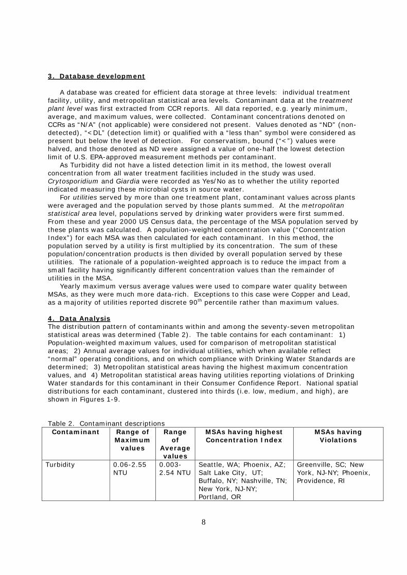
3. Database development

A database was created for efficient data storage at three levels: individual treatment facility, utility, and metropolitan statistical area levels. Contaminant data at the treatment plant level was first extracted from CCR reports. All data reported, e.g. yearly minimum, average, and maximum values, were collected. Contaminant concentrations denoted on CCRs as “N/A” (not applicable) were considered not present. Values denoted as “ND” (non-detected), “<DL” (detection limit) or qualified with a “less than” symbol were considered as present but below the level of detection. For conservatism, bound (“<”) values were halved, and those denoted as ND were assigned a value of one-half the lowest detection limit of U.S. EPA-approved measurement methods per contaminant.

As Turbidity did not have a listed detection limit in its method, the lowest overall concentration from all water treatment facilities included in the study was used. Crytosporidium and Giardia were recorded as Yes/No as to whether the utility reported indicated measuring these microbial cysts in source water.

For utilities served by more than one treatment plant, contaminant values across plants were averaged and the population served by those plants summed. At the metropolitan statistical area level, populations served by drinking water providers were first summed. From these and year 2000 US Census data, the percentage of the MSA population served by these plants was calculated. A population-weighted concentration value (“Concentration Index”) for each MSA was then calculated for each contaminant. In this method, the population served by a utility is first multiplied by its concentration. The sum of these population/concentration products is then divided by overall population served by these utilities. The rationale of a population-weighted approach is to reduce the impact from a small facility having significantly different concentration values than the remainder of utilities in the MSA.

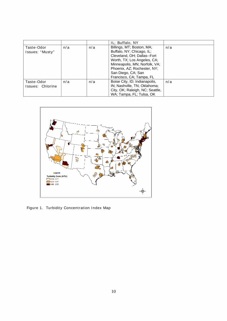
Yearly maximum versus average values were used to compare water quality between MSAs, as they were much more data-rich. Exceptions to this case were Copper and Lead, as a majority of utilities reported discrete 90th percentile rather than maximum values. 4. Data Analysis The distribution pattern of contaminants within and among the seventy-seven metropolitan statistical areas was determined (Table 2). The table contains for each contaminant: 1) Population-weighted maximum values, used for comparison of metropolitan statistical areas; 2) Annual average values for individual utilities, which when available reflect “normal” operating conditions, and on which compliance with Drinking Water Standards are determined; 3) Metropolitan statistical areas having the highest maximum concentration values, and 4) Metropolitan statistical areas having utilities reporting violations of Drinking Water standards for this contaminant in their Consumer Confidence Report. National spatial distributions for each contaminant, clustered into thirds (i.e. low, medium, and high), are shown in Figures 1-9. Table 2. Contaminant descriptions Contaminant Range of

Maximum values

Range of

Average values

MSAs having highest Concentration Index

MSAs having Violations

Turbidity 0.06-2.55 NTU

0.003-2.54 NTU

Seattle, WA; Phoenix, AZ; Salt Lake City, UT; Buffalo, NY; Nashville, TN; New York, NJ-NY; Portland, OR

Greenville, SC; New York, NJ-NY; Phoenix, Providence, RI

9

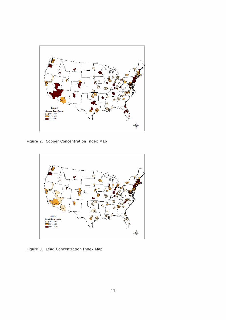
Copper 0.01-0.82 ppm

0.0005-1.3 ppm

Peoria, IL; Lincoln, NE; Boise City, ID; Orlando, FL; Los Angeles, CA; Las Vegas, NV; Huntington, WV

None

Lead 0.004-16.7 ppb

0.001-15 ppb

Louisville, KY; Springfield, MA; Billings, MT; New York, NY-NJ; Boston, MA; Fort Wayne, IN; Wichita, KS

Milwaukee, WI

Total Trihalomethanes

5-157.4 ppb

0.02-81 ppb

Phoenix, AZ; Little Rock, AR; Jacksonville, FL; Boston, MA; Mobile, AL; Tulsa, OK; Huntington, WV.

Hartford, CT; Huntington, WV; New York, NY-NJ.

Haloacetic acids 2.4-131.7 ppb

0.028-68 ppb

Phoenix, AZ; Reno, NV; Boston, MA; Washington--Baltimore, DC; Little Rock, AR; Burlington, VT Los Angeles, CA; Nashville, TN

Huntington--Ashland, WV; Jackson, MS

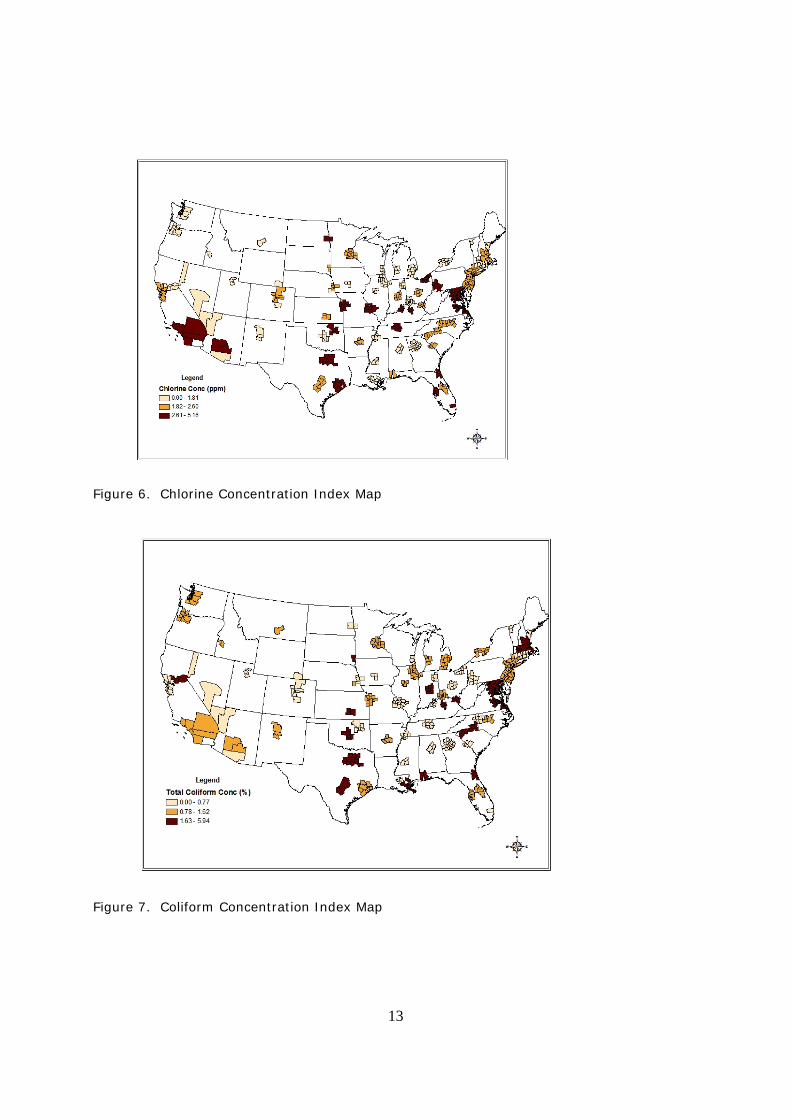
Chlorine 0.36-5.15 ppm

0.06-3.8 ppm

Norfolk, VA—NC; Richmond, VA; Nashville, TN; Washington--Baltimore, DC; Dallas--Fort Worth, TX; Los Angeles; Tampa, FL

none

Coliform 0.005-5.14 percent

0-4.42 percent

Charlotte, NC; Lexington, KY; Oklahoma City, OK; San Antonio, TX; Jacksonville, FL; Springfield, MA; Richmond, VA

Albuquerque, NM; Charlotte, NC; Dallas--Fort Worth, TX; Hartford, CT; Jacksonville, FL; Philadelphia, PA; Sacramento, CA; San Francisco, CA.

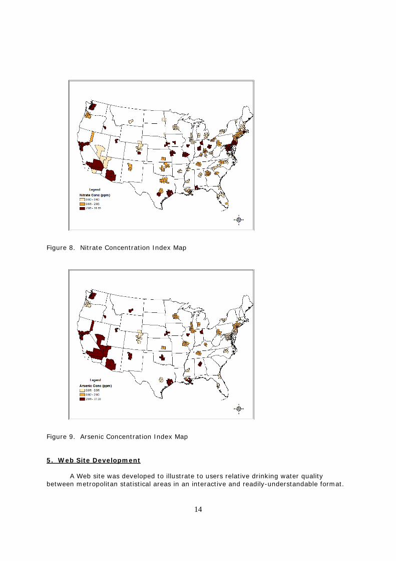
Nitrate 0.08-14.6 ppm

0.005-24 ppm

Sacramento--Yolo, CA; Des Moines, IA; Los Angeles, CA; San Francisco, CA; Lincoln, NE; Colorado Springs, CO; Mobile, AL

none

Arsenic 0.005-77 ppm

0.003-27 ppm

Oklahoma City, OK; Albuquerque, NM; Sacramento, CA; New Orleans, LA; Boise City, ID

Oklahoma City, OK

Crypotsporidium/ Giardia

Yes/No Yes/No Seattle, WA; San Francisco, CA; Sacramento, CA; Philadelphia, PA; Washington—Baltimore, DC; Pittsburgh, PA; Milwaukee, WI; Denver, CO; Atlanta, GA; Chicago,

n/a

10

IL; Buffalo, NY Taste-Odor Issues: “Musty”

n/a n/a Billings, MT; Boston, MA; Buffalo, NY; Chicago, IL; Cleveland, OH; Dallas--Fort Worth, TX; Los Angeles, CA; Minneapolis, MN; Norfolk, VA; Phoenix, AZ; Rochester, NY; San Diego, CA; San Francisco, CA; Tampa, FL

n/a

Taste-Odor Issues: Chlorine

n/a n/a Boise City, ID; Indianapolis, IN; Nashville, TN; Oklahoma; City, OK; Raleigh, NC; Seattle, WA; Tampa, FL; Tulsa, OK

n/a

Figure 1. Turbidity Concentration Index Map

11

Figure 2. Copper Concentration Index Map

Figure 3. Lead Concentration Index Map

12

Figure 4. Total Trihalomethanes Concentration Index Map

Figure 5. Total Haloacetic Acid Concentration Index Map

13

Figure 6. Chlorine Concentration Index Map

Figure 7. Coliform Concentration Index Map

14

Figure 8. Nitrate Concentration Index Map

Figure 9. Arsenic Concentration Index Map 5. Web Site Development

A Web site was developed to illustrate to users relative drinking water quality between metropolitan statistical areas in an interactive and readily-understandable format.

15

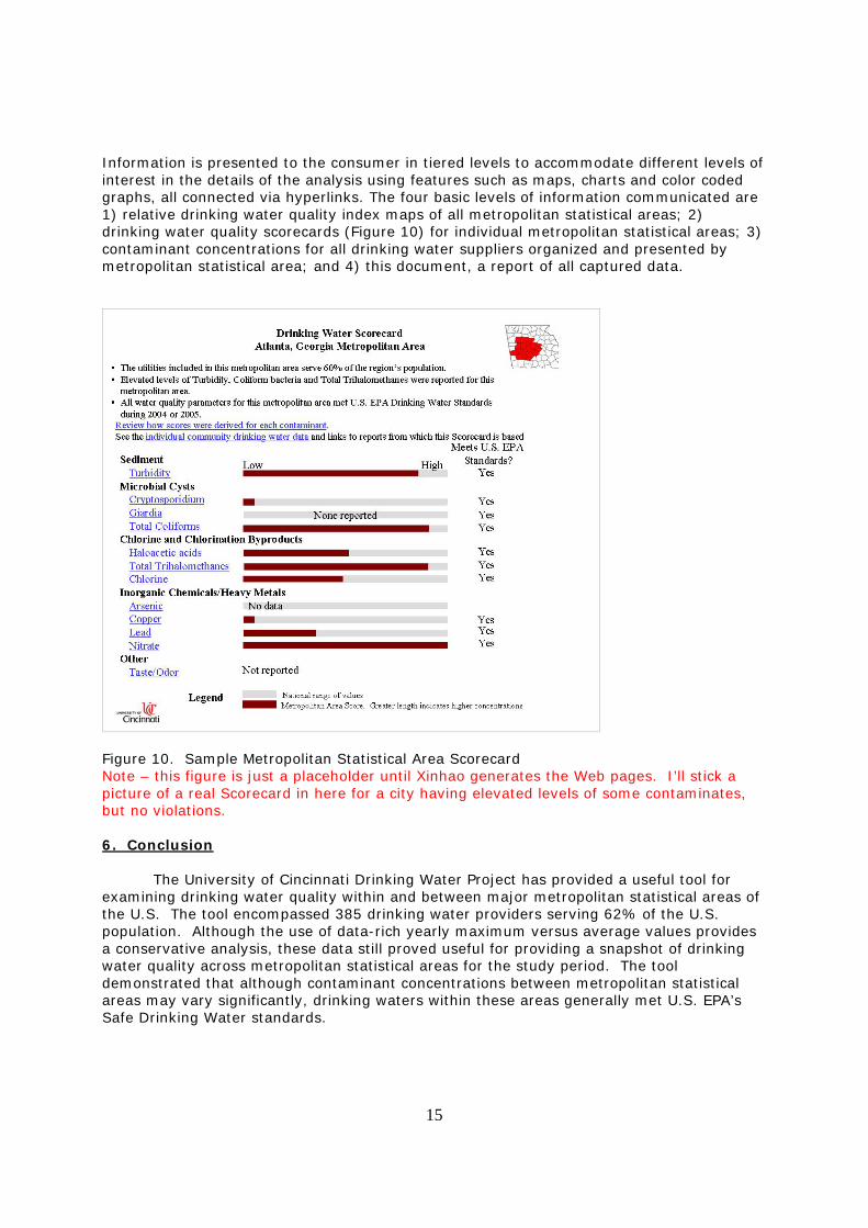
Information is presented to the consumer in tiered levels to accommodate different levels of interest in the details of the analysis using features such as maps, charts and color coded graphs, all connected via hyperlinks. The four basic levels of information communicated are 1) relative drinking water quality index maps of all metropolitan statistical areas; 2) drinking water quality scorecards (Figure 10) for individual metropolitan statistical areas; 3) contaminant concentrations for all drinking water suppliers organized and presented by metropolitan statistical area; and 4) this document, a report of all captured data.

Figure 10. Sample Metropolitan Statistical Area Scorecard Note – this figure is just a placeholder until Xinhao generates the Web pages. I’ll stick a picture of a real Scorecard in here for a city having elevated levels of some contaminates, but no violations. 6. Conclusion

The University of Cincinnati Drinking Water Project has provided a useful tool for examining drinking water quality within and between major metropolitan statistical areas of the U.S. The tool encompassed 385 drinking water providers serving 62% of the U.S. population. Although the use of data-rich yearly maximum versus average values provides a conservative analysis, these data still proved useful for providing a snapshot of drinking water quality across metropolitan statistical areas for the study period. The tool demonstrated that although contaminant concentrations between metropolitan statistical areas may vary significantly, drinking waters within these areas generally met U.S. EPA’s Safe Drinking Water standards.

16

References U.S. Environmental Protection Agency. FACTOIDS: Drinking Water and Ground Water Statistics for 2005. Office of Water. 2006. EPA 816-K-03-001 U.S. Environmental Protection Agency. National Primary Drinking Water Standards. Office of Water. 2003. EPA 816-F-03-016 U.S. Office of Management and Budget. Ranking Tables for Population of Metropolitan Statistical Areas, Micropolitan Statistical Areas, Combined Statistical Areas, New England City and Town Areas, and Combined New England City and Town Areas: 1990 and 2000. 2004. PHC-T-29 U.S. Environmental Protection Agency. System User’s Guide for SDWIS/FED. Office of Ground Water and Drinking Water. 2000, EPA/68-W-99-00.