Urban water demand forecasting and uncertainty assessment

Urban water demand forecasting and uncertainty assessment usingensemble wavelet-bootstrap-neural network models

Mukesh K. Tiwari1 and Jan Adamowski2

Received 26 July 2012; revised 20 August 2013; accepted 4 September 2013; published 9 October 2013.

[1] A new hybrid wavelet-bootstrap-neural network (WBNN) model is proposed in thisstudy for short term (1, 3, and 5 day; 1 and 2 week; and 1 and 2 month) urban waterdemand forecasting. The new method was tested using data from the city of Montreal inCanada. The performance of the WBNN method was compared with the autoregressiveintegrated moving average (ARIMA) and autoregressive integrated moving average modelwith exogenous input variables (ARIMAX), traditional NNs, wavelet analysis-based NNs(WNN), bootstrap-based NNs (BNN), and a simple na€ıve persistence index model. TheWBNN model was developed as an ensemble of several NNs built using bootstrapresamples of wavelet subtime series instead of raw data sets. The results demonstrated thatthe hybrid WBNN and WNN models produced significantly more accurate forecastingresults than the traditional NN, BNN, ARIMA, and ARIMAX models. It was also found thatthe WBNN model reduces the uncertainty associated with the forecasts, and theperformance of WBNN forecasted confidence bands was found to be more accurate andreliable than BNN forecasted confidence bands. It was found in this study that maximumtemperature and total precipitation improved the accuracy of water demand forecasts usingwavelet analysis. The performance of WBNN models was also compared for differentnumbers of bootstrap resamples (i.e., 25, 50, 100, 200, and 500) and it was found thatWBNN models produced optimum results with different numbers of bootstrap resamplesfor different lead time forecasts with considerable variability.

Citation: Tiwari, M. K., and J. Adamowski (2013), Urban water demand forecasting and uncertainty assessment using ensemblewavelet-bootstrap-neural network models, Water Resour. Res., 49, 6486–6507, doi:10.1002/wrcr.20517.

1. Introduction

[2] Effective and optimized operation and managementof urban water resources are critical [Jain and Ormsbee,2002]. Variation in urban water demand can be attributedto numerous factors such as climatic factors (temperature,rainfall, and humidity) [Altunkaynak et al., 2005; Firatet al., 2009], demographic factors (population, income,people per household, and housing density) [Zhou et al.,2002; Firat et al., 2009], public policy factors (pricing,conservation programs, and education) [Babel et al., 2007;Firat et al., 2009], industrial and commercial factors (na-ture, size, and productivity) [Zhou et al., 2002], and effi-ciency and technology [Kayaga and Smout, 2007]. Urbanwater demand management generally aims to decrease theoverall peak demand stemming from the various sourcesdescribed above.

[3] One of the main purposes of urban water demandforecasting is to match supply with demand at a servicelevel acceptable to consumers [Zhou et al., 2002]. Accurateforecasts allow for optimization of planning, design, man-agement, and operations [Firat et al., 2009], ultimatelyallowing for efficient allocation of water between compet-ing users and the ecosystem within a river basin [Altunkay-nak et al., 2005; Herrera et al., 2010]. Thus, forecastingplays a vital role in socially, economically, and environ-mentally sustainable water resources management [Caiado,2010]. Through water demand forecasting, energy use canalso be optimized, which is beneficial for both environmen-tal and economic interests [Herrera et al., 2010], especiallysince energy costs account for 25–30% of total operatingcosts [Ghiassi et al., 2008]. A distinction between short-term and long-term forecasts is usually made due to theirdifferent uses, as well as their differing modeling techni-ques. Although not specifically defined, short-term fore-casts generally include hourly, daily, and weekly forecastswith up to 48 h, 14 day, and 26 week lead times, respec-tively [Ghiassi et al., 2008]. Long-term forecasts, in com-parison, are generally annual and decadal, while monthlyforecasts, with up to 24 month lead times, are sometimesclassified as medium term. Long-term forecasts canaccount for economic, demographic, and future climatechange variables, which aid in the development, planning,and design of system infrastructure [Jain and Ormsbee,2002; Ghiassi et al., 2008; Firat et al., 2009; Herrera

1Department of Soil and Water Engineering, College of Agriculturaland Technology, Anand Agricultural University, Godhra, Gujarat, India.

2Department of Bioresource Engineering, McGill University, Ste Annede Bellevue, Quebec, Canada.

Corresponding author: J. Adamowski, Department of BioresourceEngineering, McGill University, Ste Anne de Bellevue, 21 111 LakeshoreRoad, Quebec H9X 3V9, Canada. ([email protected])

©2013. American Geophysical Union. All Rights Reserved.0043-1397/13/10.1002/wrcr.20517

6486

WATER RESOURCES RESEARCH, VOL. 49, 6486–6507, doi:10.1002/wrcr.20517, 2013

et al., 2010], as well as in the determination of effectivecombinations of various water sources to meet water quan-tity demand and quality standards [Herrera et al., 2010].Long-term forecasting is also essential for assessing theeffectiveness of conservation measures and developing pol-icies and strategies such as water pricing [Babel et al.,2007].

[4] This paper is focused on short-term urban waterdemand forecasts, which require accurate forecasts ofquick, unexpected changes, especially in daily, weekly, andmonthly forecasts. Short-term forecasts allow for optimalpump, well, reservoir, and mains operations, balanced allo-cation amongst urgent water needs, and development ofshort-term demand management strategies [Jain and Orms-bee, 2002; Kame’enui, 2003; Herrera et al., 2010]. Short-term water demand forecasts also aid in accurate decisionmaking, such as when to implement regulatory water userestrictions in times of water stress or drought [Jain andOrmsbee, 2002; Kame’enui, 2003; Herrera et al., 2010],or when to start drawing from auxiliary supplies [Jain andOrmsbee, 2002]. Urban water supply operators often makethe above operational decisions based on experience, butaccurate and reliable forecasts can ensure operations aremore attuned to demand variability [Zhou et al., 2002].Important variables in short-term urban water demand fore-cast modeling include temperature, precipitation, and pastwater demand data. Water demand exhibits a very complexrelationship with all of these input variables, and extractingnonlinearity and nonstationarity from such data is very im-portant. As such, there is a need to develop hybrid modelsthat combine different modeling approaches (that canaddress nonlinearity, nonstationarity, and uncertaintyassessment) to model water demand accurately and reli-ably. These issues are directly addressed in this paper.

[5] Short-term water demand data generally shows non-linear and nonstationary behavior [Ghiassi et al., 2008] atmultiple spatial and temporal scales [House-Peters andChang, 2011]. Short-term urban water demand shows diur-nal variation, with differing patterns for weekdays, week-ends, and holidays, while also showing longer monthly,seasonal, and yearly cycles [Zhou et al., 2002; Caiado,2010]. In the past three decades, urban water demandmodeling has increasingly addressed such behavior, aidedby increased data availability and advances in computingmethods and power [Zhou et al., 2002; Caiado, 2010].Short-term demand forecasting has traditionally usedlinear-regression models, such as multilinear regressionand autoregressive integrated moving average (ARIMA)type methods. These methods remain the most common[Adamowski and Chan, 2011], but the inability of linear-regression models to adequately account for nonlinear,nonstationary water demand data has led to the examina-tion of other methods. Zhou et al. [2002] and Jain andOrmsbee [2002] applied artificial neural networks (NN) inshort-term urban water demand forecasting to address nonli-nearity, and subsequent research has generally shown thatNNs outperform linear regression techniques in urban waterdemand forecasting [e.g., Leclerca and Ouarda; 2007; Ada-mowski, 2008; Sahoo et al., 2009; Adamowski et al., 2012].Earlier studies demonstrated that NNs have the ability tosimulate different water resources time series and to identifythe nonlinear relationship between different variables. How-

ever, NN models including other approaches such asARIMA are generally not able to perform effectively withdata that is ‘‘noisy’’ and nonstationary. NN models haveshown significant improvement with preprocessed input var-iables [Cannas et al., 2006; Wu et al., 2010; Tiwari andChatterjee, 2010b; Adamowski et al., 2012]. Over the courseof the last 10 years or so, studies have also explored thepotential of wavelet analysis to effectively decompose non-stationary data into sets of new time series at varying scalesthat can subsequently be used in forecasting models [e.g.,Cannas et al., 2006; Adamowski, 2008, 2012]. Adding thisdata decomposition step prior to feeding the wavelet decom-posed data into a NN model has been shown to furtherimprove accuracy, although the use of such hybrid wavelet-neural network (or WNN) models is still very rare in theurban water demand forecasting literature.

[6] Uncertainty in water demand forecasts arising fromdata, parameters and model structure needs to be quantifiedin terms of prediction intervals to make forecasts reliable.Data driven models including NN and WNN models aremore prone to uncertainty associated with the forecasts[Arhami et al., 2013; Tiwari et al., 2013]. To assess theuncertainty associated with the forecasts obtained usingNN and WNN models, the bootstrap technique has beenshown to be efficient compared to Bayesian approaches[Hinsbergen et al., 2009] and easy to implement in prac-tice. As such, the bootstrap approach was applied in thisstudy. In earlier studies, ensemble forecasting of waterresource variables using the bootstrap technique haveincreased the reliability of data driven techniques by reduc-ing the variance, and the generated confidence bands usingthe bootstrap method helped quantify the uncertainty asso-ciated with the forecasts [Tiwari and Chatterjee, 2010a,2011]. For effective and reliable water demand forecastingand management, it is important to know the forecast alongwith the uncertainty associated with it. Therefore, the boot-strap method was applied in study to assess the uncertaintyassociated with NN and WNN models by developing BNNand WBNN models, respectively. As discussed, this studycoupled the WNN method with bootstrapping, a statisticalapproach that allows for the quantification of uncertaintythrough intensive resampling with replacement [Tiwari andChatterjee, 2010a, 2010b]. Bootstrap-NN (BNN) andwavelet-bootstrap NN (WBNN) models have been one ofthe newest developments in the literature for discharge andflood forecasting [Sharma and Tiwari, 2009; Tiwari andChatterjee, 2010a, 2010b, 2011]. While the WBNN methodhas not yet been applied to urban demand forecasting, pre-liminary studies by one of the authors of this paper hasfound the method to be highly accurate and reliable fordaily river discharge [Tiwari and Chatterjee, 2011] andhourly flood forecasts [Tiwari and Chatterjee, 2010b].

[7] Several authors have argued that water resourcesforecasting should explore new hybrid methods that buildon the strengths of individual methods, in addition toexploring methods that try to reduce model uncertainty[Jain and Kumar, 2007; Ascough et al., 2008; Srinivasuluand Jain, 2009; Tiwari and Chatterjee, 2009; Maier et al.,2010; Tiwari et al., 2013]. In this study, an attempt is madeto incorporate these suggestions by developing hybrid mod-els that generate accurate and reliable urban water demandforecasts and that reduce uncertainty associated with the

TIWARI AND ADAMOWSKI: ENSEMBLE WATER DEMAND FORECASTING

6487

forecasts. This study presents, for the first time, the applica-tion of the BNN and WBNN method in urban waterdemand forecasting. The performance of these models isevaluated for different lead times, namely daily, weekly,and monthly forecasting, for the first time. In addition, theeffect of the number of bootstrap resamples is assessed forthe first time for water demand forecasting, and the selec-tion of an appropriate wavelet transform and the optimumnumber of decomposition levels for different lead times ofwater demand forecasting is also explored for the first time.

2. Theoretical Background

[8] A theoretical background of wavelet transforms andthe bootstrap method is provided since these are both rela-tively new methods in water resources forecasting. Sincethe autoregressive integrated moving average (ARIMA)and artificial neural network (ANN) methods are wellknown, a theoretical background of these two methods isnot provided. Adamowski [2008] and Adamowski et al.[2012] provide a detailed background of the ARIMAapproach for water resources forecasting, while Bishop[1995] and Haykin [1999] provide further explanations ofthe general properties of ANNs, and Maier and Dandy[2010] discuss various applications of ANNs in waterresources forecasting.

2.1. Wavelet Analysis

[9] The basic aim of wavelet analysis is to achieve acomplete time-scale representation of localized and tran-sient phenomena occurring at different time scales. Wave-let analysis determines the frequency (or scale) content of asignal and the temporal variation of this frequency content[Heil and Walnut, 1989]. This property of wavelet analysisis different from Fourier analysis that allows for the deter-mination of the frequency content of a signal but fails todetermine frequency time dependence. Therefore, thewavelet transform is the tool of choice when signals arecharacterized by localized high-frequency events or whensignals are characterized by a large numbers of scale-variable processes. Because of its localization properties inboth time and scale, the wavelet transform allows for track-ing the time evolution of processes at different scales in thesignal. Water demand time series are characterized by highnonlinearity and nonstationarity, with several meteorologi-cal variables and socioeconomic factors characterized bylarge numbers of scale variable processes affecting it in dif-ferent ways [Lertpalangsunti et al., 1999; Zhou et al.,2000; Jain and Ormsbee, 2002]. Wavelet analysis caneffectively decompose the original time series data intonew sets of time series data at varying scales, making non-stationarity more obvious. A brief description of waveletanalysis is described below; for more detailed informationon the theory behind wavelets interested readers aredirected to refer to Mallat [1998].

[10] The coefficients of the wavelet transform of acontinuous-time signal f(t) are defined by the linear integraloperator as

Wf a; bð Þ ¼ jaj�12

Zþ1

�1

f tð Þ � t � b

a

� �dt ð1Þ

where Wf (a, b) is the wavelet coefficient and � correspondsto the complex conjugate. The wavelet function denoted as (t), also known as the mother wavelet can be either real orcomplex. a is the scale or frequency factor controlling thedilation (a> 1) or contraction (a< 1) of the wavelet func-tion, and b is the time factor affecting the temporal transla-tion of the function.

[11] The mother wavelet function (t) has finite energyand is mathematically defined as

Zþ1

�1

tð Þdt ¼ 0: ð2Þ

[12] a,b(t), the successive wavelet, can be derived as[Kisi, 2010]

a;b tð Þ ¼ jaj�12

t � b

a

� �a 2 R; a 6¼ 0; b 2 R ð3Þ

[13] The wavelet transform searches for correlationsbetween the signal and the wavelet function at differentscales of a and locally around the time of b to form a con-tour map known as a scalogram. However, it is inefficientand impractical to compute wavelet coefficients at every re-solution level of a and b, so values corresponding to thepowers of two are often chosen for a and b. This arrange-ment of a and b is known as a dyadic grid arrangement andis the simplest and most efficient case for practical pur-poses. It can be defined as [Mallat, 1989]

m;n

t � b

a

� �¼ a�m=2

o � t � nboamo

amo

� �ð4Þ

where m and n are integers that determine the magnitude ofwavelet dilation and translation, respectively, a0 is a speci-fied dilation step greater than 1 (most commonly a0¼ 2),and b0 is the location parameter which must be greater thanzero (most commonly b0¼ 1). For a discrete time seriesf(t), assuming a0¼ 2 and b0¼ 1, the DWT simplifies as[Kisi, 2010]

Wf m; nð Þ ¼ 2�m=2XN�1

t¼0

f tð Þ � 2�mi� nð Þ ð5Þ

where Wf(m, n) is the wavelet coefficient for the DWT ofscale a¼ 2m and location b¼ 2mn. f(t) is a finite time series(t¼ 0, 1, 2, . . . , N � 1), where the maximum t¼N, definedas an M integer power of 2 (N¼ 2M). n is the time transla-tion parameter in the range 0< n< 2M–m� 1, and m is themagnitude dilation parameter with the range 1<m<M. Inthis way, a DWT performs a multilevel resolution decom-position of a time series by choosing a discrete scale (inte-ger) for m and n to develop a set of wavelet coefficients.For the largest possible wavelet scale such as 2m, wherem¼M, one DWT covers the entire time interval and gener-ates only one coefficient and at the next scale such as 2m�1,two wavelets cover the time interval, generating two coeffi-cients. The same process continues until m¼ 1 when a¼ 21

(i.e., 2M�1), and N/2 coefficients are generated. Finally, thetotal number of wavelet coefficients produced using


6488

discrete wavelet transformation for a discrete time series oflength N¼ 2M is 1þ 2þ 4þ 8þ . . . þ 2M� 1¼N� 1.Moreover, the term W can be used to denote the entire sig-nal mean, also called a signal smoothed component. Con-sidering that in wavelet analysis, a time series of length Nis broken into N components with zero redundancy, theinverse discrete transform can be described as [Nouraniet al., 2009]

f tð Þ ¼ W þXMm¼1

X2M�m�1

n¼0

Wf m; nð Þ2�m2 � 2�mi� nð Þ ð6Þ

or further simplified as [Nourani et al., 2009]

f tð Þ ¼ W tð Þ þXMm¼1

Wm tð Þ ð7Þ

where W tð Þ is the approximation subsignal at level M,and Wm(t) is the detailed subsignal at each level m¼1, 2, . . . , M.

2.2. Bootstrap Technique

[14] The bootstrap technique is a computational, data-driven method that simulates multiple realizations fromone data set of a distribution or process. A set of bootstrapsamples are created through intensive resampling withreplacement after each resampling. This expansion in thenumber of realizations provides a better understanding ofthe average and variability of the original, unknown distri-bution or process, reducing uncertainty [Efron, 1979; Efronand Tibishirani, 1993]. To combine the bootstrap methodwith NNs in this study, each resampled data set was used totrain a single NN. Assume a population of an unknownprobability distribution F, where ti¼ (xi, yi) is a realizationdrawn independently and identically distributed (i.i.d.)from F, xi is a predictor vector with yi, the correspondingoutput variable, and a n number of samples are drawn fromF, resulting in a random data set sample, denoted asTn¼ {(x1, y1), (x2, y2), . . . ., (xn, yn)}. The empirical distri-bution function for Tn is F with a mass of 1/n for each t1,t2, . . . , tn. Similar to sampling from the unknown distribu-tion F, an n number of samples of ti¼ (xi, yi) are takenfrom F that are i.i.d and then replaced. One bootstraprealization would be the resulting random sample setT� ¼ {(x1, y1), (x2, y2), . . . ., (xn, yn)}, and a set of bootstrap

samples of T1, T2, . . . , Ts, . . . , TS can be produced. The totalnumber of bootstrap samples, S, usually ranges from 50 to200 samples [Efron, 1979]. For each Ts, a NN model isdeveloped and trained using all n observations. The NNoutput, fNN xi;ws=Tsð Þ, is then evaluated using the set A ofobservation pairs ti¼ (xi, yi) that were not a part of thebootstrap sample Ts. The performance of the NNs in thesevalidation tests are subsequently averaged, which repre-sents the generalization error for the NN models relative toTn. This generalization error is denoted as E0, and this canbe estimated as [Twomey and Smith, 1998]

E0 ¼

XS

s¼1

Xi2A

yi � fNN xi;ws=Tsð Þð Þ2XS

s¼1Að Þ

ð8Þ

where fNN(xi, ws/Ts) is, again, the output of the NN developed

from the bootstrap sample Ts, in which xi is a particular inputvector and ws is the weight vector. Finally, the BNN esti-mate y xð Þ of all developed NNs is given by the average ofthe S bootstrapped estimates [Jia and Culver, 2006]

y xð Þ ¼ 1

S

XS

s¼1fNN x;ws=Tsð Þ ð9Þ

and the variance is given by

�2 xð Þ ¼

XS

s¼1

Xi¼A

yi � fNN xi;ws=Tsð Þ½ �2

S � 1ð10Þ

[15] The confidence interval (CI) at the �% significancelevel indicates that in repeated application of the technique,the frequency with which the CI would contain the truevalue is 100 � (1��)%. A typical value of � is 0.05 whichcorresponds to (1� 0.05) � 100%¼ 95% confidence lim-its. A 100 � (1��)% CI covering the mean/ensembledemand y xð Þ can be estimated using the following equation[Efron and Tibshirani, 1993]

CI ¼ UB ; LB½ � ¼ y xð Þ þ t�=2n�p� xð Þ; y xð Þ � t�=2

n�p� xð Þh i

ð11Þ

where UB is the upper band, LB is the lower band, �(x) isthe standard deviation of S bootstrapped estimates, t�=2

n�p isthe �/2 percentile for the Student t distribution with n� pdegrees of freedom, n is the total number of water demandobservations, and p is the total number of parameters in theNN model. A typical value of � is 0.05.

3. Study Area and Data

[16] Montreal is the second largest city in Canada, with apopulation of approximately 1.6 million [Statistics Canada,2007]. The city’s six drinking water treatment plants drawwater from three sources surrounding the city: Riviere desPrairies, Lake Sainte Louis, and the St. Lawrence River.The two treatment plants, Atwater and Charles-J. des Bail-lets, are some of the largest plants in Canada. They drawwater from the St. Lawrence and have the capacity to treat1364 million and 1136 million cubic meters of water perday, respectively, which comprises 88% of the entire watertreatment capacity of Montreal, [City of Montreal, 2010].Montreal’s 5000 km water distribution network is old, withapproximately 500 pipe breaks per year, some of whichremain undetected for months or years. Studies in the pastdecade have indicated that approximately 40% of thetreated water is lost, indicating a need to repair water linesand to improve water leak detection techniques. Since2002, the city has begun major rehabilitation and repairs ofthe distribution system; it has been estimated that this willtake a minimum of 20 years and cost several billions ofdollars [City of Montreal, 2010]. On average, Montreal pro-duces 2 million cubic meters of drinking water per day[City of Montreal, 2010]. Residents of the province of Que-bec and Montreal consume more water than other


6489

Canadians; one explanation for this has been the lack ofmetering within the province.

[17] In terms of weather, the average summer high inMontreal is 23�C, with a historic extreme high of 38�C,and the average winter low is �11�C, with a historicextreme low of �38�C. Annual rainfall in Montreal isalmost 1000 mm, with an extreme daily rainfall of 93.5mm. Annua snowfall averages over 200 cm with anextreme daily snowfall of 43.2 cm [Environment Canada,2010]. The data that was used in the study was provided bythe City of Montreal and consisted of average daily and av-erage monthly water demand (WatDemand), maximumtemperature (MaxT), and total precipitation (TotP).

4. Model Development

4.1. Neural Network Structure Identification

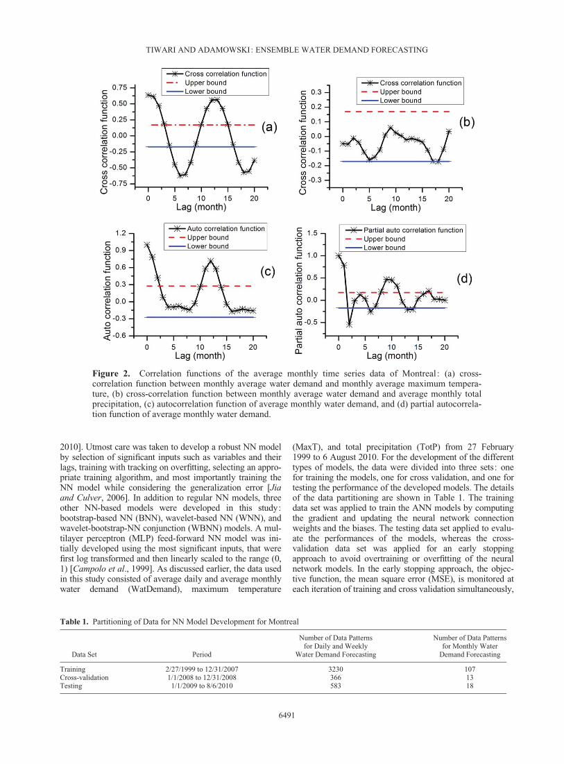
[18] Proper selection of input variables is critical in NNmodel development, as there is no direct method to select theoptimum number of inputs. In this study, a trial and errormethod was used to select the optimum number of inputsalong with a statistical approach recommended by Sudheeret al. [2002]. This statistical approach assumes that the im-portant variables for each time lag can be identified by statis-tically analyzing the data series, by examining crosscorrelations, autocorrelations, and partial autocorrelationsbetween the variables. Initially, this process was applied to

select significant inputs from the water demand data of Mon-treal for daily and monthly urban water demand forecasting.Significant inputs for weekly water demand forecasting wereselected using the same cross-correlation statistics used fordaily water demand time series. The cross-correlation statis-tics for the city of Montreal for daily time steps and monthlytime steps are shown in Figures 1 and 2, respectively. Figures1b and 2b show that precipitation does not play a significantrole in determining water demand as the correlation betweenthose two variables in Montreal is close to 0. Further, it is dif-ficult to select significant inputs for maximum temperatureand water demand lags using the cross-correlation statistics,because the correlation is not found to be significant. Thus, atrial and error procedure was adopted to determine the signif-icant input variables. In this study, the number of hidden neu-rons that produced the lowest generalization error wasdetermined to be the optimal structure [Jia and Culver,2006]. For water demand forecasting in Montreal at differentlead times, past information of water demand, total precipita-tion, and maximum temperature were considered, and theNN structures were tested for 1–14 hidden neurons.

4.2. NN, BNN, WNN, WBNN, ARIMA, and ARIMAXModel Development

4.2.1. NN Model Development[19] All the methodological issues need to be considered

for the development of a robust NN model [Maier et al.,

Figure 1. Correlation functions of the daily time series data of Montreal: (a) cross-correlation functionbetween daily water consumption and daily maximum temperature, (b) cross-correlation functionbetween daily water consumption and daily total precipitation, (c) autocorrelation function of daily waterconsumption, and (d) partial autocorrelation function of daily water consumption.


6490

2010]. Utmost care was taken to develop a robust NN modelby selection of significant inputs such as variables and theirlags, training with tracking on overfitting, selecting an appro-priate training algorithm, and most importantly training theNN model while considering the generalization error [Jiaand Culver, 2006]. In addition to regular NN models, threeother NN-based models were developed in this study:bootstrap-based NN (BNN), wavelet-based NN (WNN), andwavelet-bootstrap-NN conjunction (WBNN) models. A mul-tilayer perceptron (MLP) feed-forward NN model was ini-tially developed using the most significant inputs, that werefirst log transformed and then linearly scaled to the range (0,1) [Campolo et al., 1999]. As discussed earlier, the data usedin this study consisted of average daily and average monthlywater demand (WatDemand), maximum temperature

(MaxT), and total precipitation (TotP) from 27 February1999 to 6 August 2010. For the development of the differenttypes of models, the data were divided into three sets: onefor training the models, one for cross validation, and one fortesting the performance of the developed models. The detailsof the data partitioning are shown in Table 1. The trainingdata set was applied to train the ANN models by computingthe gradient and updating the neural network connectionweights and the biases. The testing data set applied to evalu-ate the performances of the models, whereas the cross-validation data set was applied for an early stoppingapproach to avoid overtraining or overfitting of the neuralnetwork models. In the early stopping approach, the objec-tive function, the mean square error (MSE), is monitored ateach iteration of training and cross validation simultaneously,

Figure 2. Correlation functions of the average monthly time series data of Montreal: (a) cross-correlation function between monthly average water demand and monthly average maximum tempera-ture, (b) cross-correlation function between monthly average water demand and average monthly totalprecipitation, (c) autocorrelation function of average monthly water demand, and (d) partial autocorrela-tion function of average monthly water demand.

Table 1. Partitioning of Data for NN Model Development for Montreal

Data Set Period

Number of Data Patternsfor Daily and Weekly

Water Demand Forecasting

Number of Data Patternsfor Monthly Water

Demand Forecasting

Training 2/27/1999 to 12/31/2007 3230 107Cross-validation 1/1/2008 to 12/31/2008 366 13Testing 1/1/2009 to 8/6/2010 583 18


6491

and the training is stopped at the point the MSE for thecross-validation data reaches the minimum level. After thislevel, the NN model will start overfitting despite better per-formance (e.g., decreasing MSE) during training [Bishop,1995]. To increase computational efficiency, a second-ordertraining method, the Levenberg-Marquardt method, was usedto minimize the mean squared error between the forecastedand observed water demands. All four NN-based modelswere developed with Matlab codes using MATLABVR

(v.7.10.0), except for the generation of realizations of thetraining data set to develop BNN and WBNN models, whichwas done using an Excel add-in (Bootstrap.xla) [Barreto andHowland, 2006].

[20] The NN models (i.e., NN, BNN, WNN, and WBNN)were developed using daily average water demand, dailymaximum temperature, daily average total precipitation for1, 3, and 5 day lead time water demand forecasting. Forweekly water demand forecasting, instead of weekly averagewater demand, weekly maximum temperature, and weeklyaverage total precipitation for 1 and 2 week lead times, dailyaverage water demand, and daily maximum temperature for1 and 2 week (i.e., 7 and 14 day) lead times was forecasted.It should be noted that when we refer to weekly forecastingin this study, the aim was to forecast for exactly the sameday the following week. This was done since it was deemedto be more useful to forecast water demand for the same day1 week ahead (and the same day 2 weeks ahead) given thatwater demand varies depending on the day (for example,whether it is a week day or a weekend day), instead of fore-casting total average 1 week and 2 week water demand.Monthly water demand for 1 and 2 months was forecastedusing monthly average water demand, monthly average max-imum temperature, and monthly average total precipitation.4.2.2. WNN Model Development

[21] Next, the WNN model was developed by inputtingthe wavelet subtime series, produced using the discretewavelet components (DWCs) at varying scales, into theNN model. Each of these subtime series plays a distinctrole in describing the original water demand series. Thewavelet functions used in this research are Haar, Daube-chies (i.e., db2, db3, db4, db5, db6), Sym3, and Coif1[Nourani et al., 2009; Wu et al., 2009], and 1–5 levels ofdecomposition were considered in this study. As the per-formance of the db5 function derived from the family ofDaubechies wavelets with three levels of decompositionwas found to be the best, for illustration purposes three lev-els of decomposition (d1, d2, and d3) and approximation(A3) for the daily and monthly water demand and tempera-ture data of Montreal are shown in Figures 3 and 4, respec-tively. As explained earlier, it should be noted thatdecomposed daily time series data were also used to de-velop models for weekly water demand forecasting with 7and 14 day (i.e., 1 week and 2 week) lead times, respec-tively. The effective wavelet subtime series were deter-mined using the correlation coefficients between eachwavelet component and the observed water demand. Table2 shows the correlation between the original daily andmonthly time series and the corresponding different wave-let subtime series for Montreal. In earlier studies [Tiwariand Chatterjee, 2010b, 2011; Kisi, 2010; Adamowski andSun, 2010], the significant wavelet subtime series of a par-ticular time series were added and used, which became the

new inputs to develop the WNN model. In this study, incontrast to previous studies, considering that all the waveletsubtime series may play a significant role in the originaltime series, instead of selecting on the basis of a particularthreshold level, all the components were given due consid-eration to evaluate their effectiveness to forecast waterdemand in the city of Montreal. The performance of thedeveloped models was evaluated using five performanceindices, namely: coefficient of determination (R2), root-mean-square error (RMSE), percentage deviation in peak(Pdv), mean average error (MAE), and persistence index(PI). Persistence index (PI) is one minus the ratio of thesum square error to what the sum square error would havebeen if the forecast had been the last observed value.4.2.3. BNN Model Development

[22] The BNN model was developed as an ensemble of100 NNs built using bootstrap resamples of raw data sets(i.e., the significant input variables identified when devel-oping the NN models), whereas the WBNN model wasdeveloped as an ensemble of 100 NNs built using bootstrapresamples of wavelet subtime series (i.e., the significantinput variables identified when developing the WNN mod-els), instead of raw data sets. Thus, for a given lead time,there were 100 forecasts from a single testing data set or, inother words, by using the bootstrap technique, each leadtime had 100 sets of weights instead of one. The 100 fore-casted values for each lead time were used to build 95%confidence bands that depict the uncertainty associatedwith the forecasts.4.2.4. WBNN Model Development

[23] The WBNN model takes advantage of the capabil-ities of both the bootstrap resampling and wavelet trans-form techniques. To maintain consistency with the BNNmodel, the WBNN model was also developed using 100resamples of the same significant input variables identifiedwhen developing the WNN models. Bootstrap.xla, an Exceladd-in [Barreto and Howland, 2006], was used to generatebootstrap resamples of raw data sets for the BNN modelsand wavelet subtime series for the WBNN models. The per-formance of the best model was also tested using differentnumbers of bootstrap resamples (i.e., 25, 50, 200, and 500)to evaluate the effectiveness of the number of bootstrapresamples used. The BNN and WBNN models were used toassess and quantify the uncertainty associated with the 1, 3,and 5 day, 1 and 2 week, and 1 and 2 month lead time fore-casts by developing confidence bands using the ensembleforecasts.4.2.5. ARIMA and ARIMAX Model Development

[24] ARIMA and ARIMAX models (i.e., ARIMA mod-els with additional independent input variables) weredeveloped to forecast water demand in the city of Montrealas a benchmark to evaluate the performance of the differentNN models and were developed using the SPSS softwarepackage (version 10, SPSS Inc., Chicago, Illinois). Initially,the stationarity of the input data series was determined bythe autocorrelation function (ACF). It was observed thaturban water demand data from Montreal was nonstationary.Therefore, the data sets for ARIMA and ARIMAX model-ing were transformed into a stationary time series throughthe differencing process. The development of the ARIMAmodels in this study followed the methodology used byAdamowski [2008, 2012].


6492

5. Results and Discussion

5.1. Daily Water Demand Forecasting

5.1.1. Daily Water Demand Forecasting Using NNModels

[25] The performance of the best NN model is presentedin terms of different performance indices for 1, 3, and 5day lead times in Table 3 and Figure 5. Daily precipitationand daily maximum temperature were not found to have asignificant impact on daily lead time water demand fore-casting. The daily time step performance is satisfactory upto 5 day lead time forecasts in terms of the differentperformance indices. For 1 day lead time forecasts, it canbe observed from the scatter plots that the performance isgood for low, medium, and high demand profiles, but for 3and 5 days the performance deteriorates significantly forhigher demand profiles. It is obvious that for higher leadtimes, model performance deteriorates, as there is less in-

formation available for longer lead time horizons, but thedeteriorating performance specifically for higher values atlonger lead times shows the weakness of the NN modelstructure to forecast the higher water demand values inMontreal. Another reason may be that the number of waterdemand values is lower for high water demand values com-pared to low and medium water demand values, and theNN models try to dampen the high and medium demandvalues and underestimate the values. This indicates thatNN models are not very effective in capturing the nonsta-tionarity in the data and show the weakness of the NNmodel structure.5.1.2. Daily Water Demand Forecasting Using BNNModels

[26] To improve the performance of NN models, BNNmodels were developed by generating ensemble forecastsof water demand in Montreal for 1, 3, and 5 day lead times.Considering the range of variation of water demand in

Figure 3. Wavelet subtime series of the (a) daily water demand and (b) daily maximum temperature ofMontreal from 27 February 1999 to 6 August 2010.


6493

Montreal during the testing period from a high of 431.67ML/d to a low of 318.12 ML/d, the BNN model withRMSE values of 6.06, 10.70, and 12.55 ML/d performedwell for 1, 3, and 5 day lead times (Table 3 and Figure 5),respectively. The BNN model simulated the higher waterdemand values better than NN models for 3 and 5 day leadtimes forecasts. It can be observed from the scatter plotsthat compared to the best NN model, for 1, 3, and 5 daylead times the BNN model performed better for higherwater demand values. However, the BNN model underesti-mated several higher water demand values, especially forhigher lead time forecasts. The BNN model has thecapability to produce more stable solutions by producingensemble forecasts ; however, it is not able to extractthe nonstationarity from the data set. Considering the needto improve model performance, WNN models weredeveloped.

5.1.3. Daily Water Demand Forecasting Using WNNModels

[27] For daily water demand forecasting, the perform-ance of WNN models in terms of R2, RMSE, PI, and MAEfor all 1, 3, and 5 day lead time forecasts is much bettercompared to the best NN and BNN models (Table 3 andFigure 5). The better performance of the WNN model maybe due to the reason that NN and BNN models have limita-tions to extract the nonstationarity and the physical struc-ture from the training data set. It can be observed from thescatter plots that the WNN model simulates the observedvalues very well compared to the NN and BNN model fore-casts. Wavelet analysis simplifies the physical structure ofthe data, simplifying the learning process of WNN modelsduring training. This allows for better simulation of theobserved values, even for higher water demand valueswhose numbers are much lower in the training data set. It

Figure 4. Wavelet subtime series of the (a) monthly average water demand and (b) monthly averagemaximum temperature of Montreal from February 1999 to July 2010.


6494

can be noted that the BNN model produces more stableforecasts by combining forecasts made using differentrealizations of the training data set, whereas the WNNmodel reduces noise and extracts nonstationarity from thetraining data set. To further enhance the performance of theNN model, a hybrid WBNN model was developed by com-bining the strength of BNN and WNN models.

5.1.4. Daily Water Demand Forecasting Using WBNNModels

[28] The WBNN models, which use the capabilities ofboth the WNN and BNN models, performed very well (Ta-ble 3 and Figure 5). The performance of the best WNN andWBNN models was found to be better compared to the bestNN and BNN models. The performance of the best WNNmodel was found to be better than the WBNN model for 1and 3 day lead times, whereas the WBNN model performedbetter for 5 day lead time forecasts. The overall perform-ance of the WBNN models was considered better comparedto the best WNN models. The forecasts obtained using theWBNN models are more accurate as the bootstrap tech-nique reduces the variance, and wavelet analysis reducesthe noise, making the periodic information more obvious.Further, the different forecasts obtained from the WBNNmodel can be used to develop confidence bands to assessthe uncertainty associated with the forecasts.5.1.5. Daily Water Demand Forecasting UsingARIMA and ARIMAX Models

[29] It was observed that the inclusion of additionalinputs, namely temperature and precipitation, by develop-ing ARIMAX models does not improve the performance interms of different performance indices (Table 3), since the

Table 3. Performance of the Best Models Using NN, BNN, WNN, WBNN, ARIMA, and ARIMAX Models for 1, 3, and 5 Day LeadTime Water Demand Forecasting in Montreala

Lead Time

Best Model Structure Performance Indices

Hidden Neurons (HN) R2 RMSE (ML/d) Pdv (%) MAE (ML/d) PI

NN1 day WatDmand(t), WatDmand(t-1) WatDmand(t-2).

WatDmand(t-3) WatDmand(t-4) WatDmand(t-5)WatDmand(t-6),WatDmand(t-7),WatDmand(t-8)WatDmand(t-13)

13 0.92 5.88 0.88 4.17 0.45

3 day WatDmand(t), WatDmand(t-1) WatDmand(t-2).WatDmand(t-3) WatDmand(t-4) WatDmand(t-5)WatDmand(t-6),WatDmand(t-7)

5 0.77 9.92 2.52 7.15 0.41

5 day WatDmand(t), WatDmand(t-1) WatDmand(t-2).WatDmand(t-3) WatDmand(t-4) WatDmand(t-5)WatDmand(t-6),WatDmand(t-7),WatDmand(t-8)

11 0.71 10.91 4.80 7.11 0.37

BNN1 day Same inputs as in NN 0.90 6.09 1.66 4.41 0.413 day Same inputs as in NN 0.76 10.70 2.42 7.96 0.315 day Same inputs as in NN 0.64 12.55 0.07 9.14 0.07

WNN1 day a3(t), d3(t), d2(t), d1(t) components of WatDmand(t) 0.98 3.11 �0.57 2.21 0.843 day a3(t), d3(t), d2(t), d1(t) components of WatDmand(t) 0.94 5.33 �0.82 4.17 0.835 day a3(t), d3(t), d2(t), d1(t) components of WatDmand(t) 0.90 7.81 0.37 6.30 0.68

WBNN1 day Same inputs as in WNN 0.98 4.09 �0.97 2.99 0.733 day Same inputs as in WNN 0.96 6.08 1.04 4.81 0.785 day Same inputs as in WNN 0.90 7.29 0.54 5.82 0.72

ARIMA1 day 0.90 6.51 0.58 4.85 0.333 day 0.70 10.55 1.32 7.60 0.305 day 0.59 14.57 0.79 11.33 0.12

ARIMAX1 day 0.91 6.55 2.70 4.72 0.393 day 0.71 10.42 1.4 7.44 0.375 day 0.64 11.44 2.25 8.83 0.41

aWatDmand (tþ 1)¼ 1 day/week/month lead water demand forecast; WatDmand(t)¼Total water demand at time (t).

Table 2. Correlations Between Different Wavelet Subtime Seriesand the Original Water Demand Time Series in Montreal

Wavelet Subtime Series

Daily

WatDmand MaxT TotP

A3 0.94 0.58 �0.08D1 0.16 0.03 �0.02D2 0.25 0.06 �0.01D3 0.19 0.07 �0.02Original 1.00 0.58 �0.06

MonthlyA3 0.55 0.20 �0.09D1 0.18 0.04 0.00D2 0.42 �0.11 �0.08D3 0.69 0.65 0.10Original 1.00 0.64 �0.05


6495

Fig

ure

5.S

catt

erpl

ots

for

obse

rved

and

pred

icte

dw

ater

dem

and

inM

ontr

eal

for

1da

y,3

day,

and

5da

yle

adti

me

fore

cast

sfo

rth

ete

stin

gda

tase

tus

ing

:(a

)N

N,(

b)B

NN

,(c)

WN

N,a

nd(d

)W

BN

Nm

odel

s.


6496

performance of both ARIMA and ARIMAX models arevery similar, with the ARIMAX model performing slightlybetter than the ARIMA model for 3 and 5 the day lead timeforecasts. These exogenous inputs may increase the modelperformance for longer lead times. Overall, for daily fore-casting (1, 3, and 5 days), the performance of the WBNNmodels was found to be more accurate and reliable than theNN, BNN, WNN, ARIMA, and ARIMAX models.

5.2. Weekly Water Demand Forecasting

5.2.1 Weekly Water Demand Forecasting Using NNModels

[30] Weekly water demand forecasting for 1 week and 2week lead times was carried out using NN, BNN, WNN,WBNN, ARIMA, and ARIMAX models, and the perform-ance of the different models is presented in Table 4 andFigure 6. It can be observed in the case of weekly waterdemand forecasts that daily precipitation and daily maxi-mum temperature play a significant role and improvedmodel performance. Performance of the traditional NNmodels in terms of different performance indices for1 week lead time water demand forecasting can be consid-ered satisfactory. Further, even though the observed andforecasted values using the NN model are very close for2 week lead time forecasts, lower and medium values areoverestimated whereas peak values are underestimated.This shows that the performance of the NN model is not ac-ceptable for 2 week lead time forecasts. The performancein terms of persistence index (PI) shows that even thoughthe NN model can forecast better than a simple na€ıve per-sistence model, there is a need to apply hybrid approaches

to improve the performance of NN models for higher stepweekly water demand forecasting.5.2.2. Weekly Water Demand Forecasting Using BNNModels

[31] The performance of BNN models was found to bevery close to NN models, and both the models lacked gen-eralization capabilities (Table 4 and Figure 6) as severalvalues were overestimated or underestimated (especiallyfor 2 week lead time forecasts). This reflects the inabilityof NN models to capture the nonstationarity from the inputand output variables for longer lead time forecasts. The sig-nificant deviation from the 1:1 line for different waterdemand values shows that NN and BNN models have lim-ited capability to extract nonstationarity from the data set,and lack generalization ability as peak values are dampenedtoward frequently occurring lower and medium waterdemand values.5.2.3. Weekly Water Demand Forecasting Using WNNModels

[32] The performance of WNN models was tested for 1week and 2 week lead time forecasts and the performancein terms of different performance indices and scatter plots(Table 4 and Figure 6) showed that WNN model forecastsfor both 1 and 2 week lead times is much better comparedto the best NN and BNN models. The best WNN modelperformed well, since the forecasted values are very closeto the 1:1 line, even for the 2 week lead time water demandforecasts. Performance of the WNN model was signifi-cantly better than the NN model for 2 week lead time fore-casts; this shows that for longer lead time forecasts that arehighly affected by nonstationarity (i.e., trends and

Table 4. Water Demand Forecasting in Montreal for 1 and 2 Week Lead Times using NN, BNN, WNN, WBNN, ARIMA, and ARI-MAX Models

Lead Time Best Model Structure HN R2 RMSE (ML/d) Pdv (%) MAE (ML/d) PI

NN1 week WatDmand(t), WatDmand(t-6), MaxT(t), MaxT

(t-6), TotP(t), TotP(t-6)5 0.67 11.83 4.07 8.59 0.12

2 week WatDmand(t), WatDmand(t-6), MaxT(t), MaxT(t-6), TotP(t), TotP(t-6)

8 0.59 17.59 2.09 14.45 0.17

BNN1 week Same inputs as in NN 0.68 12.33 3.15 9.17 0.102 week Same inputs as in NN 0.57 18.02 2.75 15.22 0.12

WNN1 week a3(t), d3(t), d2(t), d1(t) of TotCons; A3 and d3 of

MaxT and A3 of TotP with 1,2 and 3 day lag timevariables

5 0.76 12.07 �1.76 8.90 0.35

2 week a3(t), d3(t), d2(t), d1(t) of TotCons; A3 and d3 ofMaxT and A3 of TotP with 1 and 7 day lag timevariables

3 0.72 15.49 �0.14 10.93 0.28

WBNN1 week Same inputs as in WNN 0.78 10.06 �0.58 7.49 0.462 week Same inputs as in WNN 0.68 18.76 1.47 16.28 0.23

ARIMA1 week 0.68 11.74 0.03 7.49 0.102 week 0.52 16.95 4.36 14.46 0.15

ARIMAX1 week 0.68 11.89 2.52 8.80 0.092 week 0.51 17.03 3.90 14.58 0.14


6497

Fig

ure

6.S

catt

erpl

ots

for

obse

rved

and

pred

icte

dw

ater

dem

and

inM

ontr

eal

for

1w

eek

and

2w

eek

lead

tim

efo

reca

sts

for

the

test

ing

data

set

usin

g:

(a)

NN

,(b)

BN

N,(

c)W

NN

,and

(d)

WB

NN

mod

els.


6498

seasonality), wavelet analysis can be used to improve themodel performance.5.2.4. Weekly Water Demand Forecasting UsingWBNN Models

[33] The performance of the best WNN and WBNNmodels was better compared to the best NN and BNN mod-els (Table 4 and Figure 6). The performance of the bestWNN model was found to be better than the WBNN modelfor 2 week lead times, whereas the WBNN model per-formed better for 1 week lead time forecasts. The overallperformance of the WBNN models was considered bettercompared to the best WNN models. The forecasts obtainedusing the WBNN model are more accurate than NN, BNN,WNN, ARIMA, and ARIMA models because the bootstraptechnique reduces the variance, and wavelet analysisreduces the noise and makes the periodic information moreeasily understandable by the model. The WBNN modelprovides more reliable forecasts since they are obtainedusing different realizations of the training data set that aver-ages over the error. Further, similar to BNN models, thedifferent forecasts obtained from the WBNN models can beused to develop confidence bands to assess the uncertaintyassociated with the forecasts.5.2.5. Weekly Water Demand Forecasting UsingARIMA and ARIMAX Models

[34] Compared to daily water demand forecasting whereinclusion of exogenous variables (i.e., daily maximum tem-perature and daily total precipitation) in the ARIMAXmodel improved the model performance compared to theARIMA model (Table 4), the inclusion of maximum tem-perature and total precipitation in the ARIMAX modeldoes not improve the model performance for 1 and 2 weeklead time water demand forecasting. Performance of the

ARIMA and ARIMAX models were very close to that ofthe NN and BNN models; however, their performance wassignificantly worse than the WNN and WBNN models.

5.3. Monthly Water Demand Forecasting in Montreal

5.3.1. Monthly Water Demand Forecasting Using NNModels

[35] Monthly water demand forecasting for 1 and 2 monthlead times was carried out using NN, BNN, WNN, WBNN,ARIMA, and ARIMAX models, and it was observed that inmonthly average water demand forecasting, monthly averagetotal precipitation, and monthly average maximum tempera-ture play a significant role and improved model performance(Table 5 and Figure 7). Considering the range of variation ofaverage monthly water demand in Montreal (a high of 388.6ML/month to a low of 328.7 ML/month), the performance ofthe regular NN model for monthly time steps and with aRMSE value of 22.18 and 24.27 ML/month cannot be con-sidered satisfactory for 1 and 2 month lead times, respec-tively. It can also be observed from the scatter plots thatregular NN models are not able to simulate the monthly aver-age water demand values satisfactorily since the valuesdiverge from the 1:1 line. Moreover, the lower values areoverestimated and the higher value is underestimated.5.3.2. Monthly Water Demand Forecasting UsingBNN Models

[36] The results for forecasts of water demand in Mon-treal for 1 and 2 month lead times show that the perform-ance of the BNN models is very similar to the NN models(Table 5 and Figure 7), and the performance of both theNN and BNN models cannot be considered satisfactory interms of the different performance indices. It can also beseen from the scatter plots that the BNN model does not

Table 5. Monthly Water Demand Forecasting in Montreal for 1 and 2 Months Lead Times Using NN, BNN, WNN, WBNN, ARIMA,and ARIMAX Models

Lead Time Best Model Structure HN R2RMSE

(ML/month) Pdv (%)MAE

(ML/month) PI

NN1 month WatDmand(t), WatDmand(t-11), Maxt(t), Maxt(t-11),

TotP(t), TotP(t-11)2 0.87 22.18 4.51 20.31 0.06

2 month WatDmand(t), WatDmand(t-10), Maxt(t), Maxt(t-11),TotP(t), TotP(t-11)

8 0.70 24.27 4.69 22.33 0.54

BNN1 month Same inputs as in NN 0.77 21.74 3.84 19.70 0.102 month Same inputs as in NN 0.74 23.03 4.34 20.97 0.58

WNN1 month A3, d1, d2, d3 components of WatDmand(t), A3 and d3

components of MaxT(t) and d3 component of TotP(t)3 0.96 5.94 �0.33 4.82 0.81

2 month A3, d1, d2, d3 components of WatDmand(t), A3 and d3components of MaxT(t) and d3 component of TotP(t)

5 0.91 7.21 0.23 5.99 0.89

WBNN1 month Same inputs as in WNN 0.77 11.13 �0.68 8.62 0.322 month Same inputs as in WNN 0.54 13.49 2.25 10.94 0.61

ARIMA1 month 0.57 16.98 4.29 14.86 0.472 month 0.67 19.68 2.99 17.70 0.69

ARIMAX1 month 0.90 19.20 �4.06 18.21 0.322 month 0.90 18.62 �3.94 17.61 0.72


6499

Fig

ure

7.S

catt

erpl

ots

for

obse

rved

and

pred

icte

dda

ily

wat

erde

man

din

Mon

trea

lfo

r1

mon

than

d2

mon

thle

adti

me

fore

cast

sfo

rth

ete

stin

gda

ta-

sets

usin

g:

(a)

NN

,(b)

BN

N,(

c)W

NN

,and

(d)

WB

NN

mod

els.


6500

simulate the water demand values satisfactorily as thesimulated values diverge from the 1:1 line. This againillustrates that NN models lack the ability to extract nonsta-tionarity from the training data set.5.3.3. Monthly Water Demand Forecasting UsingWNN Models

[37] WNN models were also used to forecast waterdemand in Montreal for 1 and 2 month lead times, and theperformance was much better compared to the best NN andBNN models (Table 5 and Figure 7). The performance ofthe WNN models with a monthly time step and with aRMSE value of 5.94 and 7.21 ML/month can be consideredvery good for 1 and 2 month lead times, respectively. It canalso be observed that the WNN model simulated the valuesvery well as the values are very close to the 1:1 line. Moreimportantly, all the values (high and low) are simulatedvery well and there is no significant evidence of underesti-mation and overestimation of water demand values as canbe observed from scatter plots.5.3.4. Monthly Water Demand Forecasting UsingWBNN Models

[38] In the case of monthly water demand forecasting,the WBNN model with a RMSE value of 13.49 ML/monthperformed well up to a 2 month lead time forecast (Table 5and Figure 7). The performance of the best WNN andWBNN models was better compared to the best NN andBNN models, with the best WNN model providing betterresults than the WBNN model. However, overall the per-formance of the WBNN models can be considered bettercompared to the best WNN models. The forecasts obtainedusing the WBNN model are more accurate because thebootstrap technique reduces the variance, and wavelet anal-ysis reduces the noise and makes the periodic informationmore readily understandable by the model.5.3.5. Monthly Water Demand Forecasting UsingARIMA and ARIMA Models

[39] The performance of the ARIMA and ARIMAXmodels was found to be better than the NN model andBNN models, but not better than the WNN and WBNNmodels (Table 5). The better performance of the ARIMAXmodel compared to the ARIMA model for a 2 month leadtime shows the significance of exogenous inputs for model-ing longer lead time water demand forecasts.

5.4. Discussion

5.4.1. Comparative Performance of the Models[40] It was observed that NN models are not able to

extract the nonstationarity from the data set. Moreover, theNN models demonstrated their weakness to extract the non-linearity when the length of the training data set is small, asit was noticed that the length of the data set is too small(i.e., net 107 data patterns) in NN, BNN, WNN, andWBNN models for 1 and 2 month lead time forecasts fortraining compared to the data patterns used for daily andweekly water demand forecasting (i.e., net 3230 data pat-terns in NN, BNN, WNN and WBNN models for 1,3, and5 day; and 1 and 2 week lead time forecasts for training).Due to the higher number of data patterns the NN and BNNmodels simulated the observed values much better for thedaily and weekly lead time forecasts; the performance ofthe NN and BNN models was not very good for monthlylead time forecasts. This may be due to the dominance of

nonstationarity in monthly water demand time series. Thisshows that the NN models and BNN models (which areensembles of different NN models) have limited capabilityto extract the nonstationarity from the data sets. Further, itcan be observed that the performance of WNN and WBNNmodels (which are the ensembles of several WNN models)are much better compared to NN and BNN models. This isbecause wavelet transform decomposed components oftime series data extract different time varying components(i.e., trends and nonstationarity) (Figures 3 and 4) that maybe representative of the sum of the subprocesses associatedwith the original time series data set. These different com-ponents facilitate the ability of the NN models that useWTs (i.e., WNN and WBNN) to extract nonlinearity andnonstationarity, and therefore their performance is superiorto NN models developed using raw data sets.

[41] The results show the advantages of using wavelets inNN models, especially as the lead time increases. The mod-els developed without wavelet transformed data consistentlyunderestimated higher water demand values, especially atlonger lead times. Accurately forecasting these high peakdemands is operationally very important. Although the useof bootstrapping did not improve model performance, over-all its additional capacity to reduce uncertainty is consideredadvantageous, outweighing the slight reduction in perform-ance seen at some lead times. The performance of theWBNN method was comparable to the WNN method for 1and 3 day lead time water demand forecasts, and theWBNN model performed slightly better for 5 day lead timeforecasts. For 1 and 2 week water demand forecasting per-formance, the WBNN and WNN models, respectively, werefound to be the best compared to the remaining models. Forof 1 and 2 month water demand forecasting, the perform-ance of the WNN model was found to be the best comparedto the remaining models.

[42] It should be noted that in some of the cases theWNN models performed better than WBNN models, butthe WBNN models are more consistent and reliable com-pared to WNN models, considering that they are an ensem-ble of several WNN models developed using differentrealizations of the training data set, and thus provide fore-casts with reduced variance (i.e., reduced uncertainty). Thenarrow confidence bands of the WBNN models, along withthe higher number of values inside the confidence bandsenables the WBNN models (for daily, weekly, and monthlywater demand forecasting) to be the most reliable methodcompared to the other methods. This is due to the reasonthat the WBNN models use the capability of wavelet analy-sis, which reduces the noise, and bootstrap resampling,which reduces the variance. The performance of the WBNNmodels is considered more reliable and accurate than theWNN models, even though in some cases the WNN modelsperformed slightly better than the WBNN models. The rea-son is that WBNN models are an ensemble of WNN modelsdeveloped using 100 realizations of the training data set,and not merely an ensemble of some selected better per-forming WNN models out of these 100 forecasts. WBNNmodels developed using different realizations of waveletsubtime series data may be representing different processesassociated with water demand simulations at different time-frequency domains, and the WBNN models average overthe error and produce more accurate and reliable forecasts.


6501

[43] The performance of ARIMA and ARIMAX modelswere found to be better than NN and BNN models forweekly and monthly water demand forecasting. The betterperformance of ARIMA and ARIMAX models comparedto NN and BNN models for weekly and monthly forecastsmay be because NN models are not very effective at captur-ing nonstationarity in the data set, and longer time step(i.e., weekly and monthly) time series data shows trend andnonstationarity, as can be observed in Figure 2. ARIMAand ARIMAX models are able to extract this nonstationar-ity from the data set and provide better forecasts than NNand BNN models. However, after decomposing the data setusing wavelet analysis by extracting the trend and nonsta-tionarity, the performance of WNN and WBNN modelsimproved significantly as discussed earlier. Moreover, thecomputation time using WBNN models proposed in thisstudy is approximately 3–5 min using average system con-figurations such as an Intel Core i5 processor with 3GBRAM. This can be considered to be a time efficient process,and the proposed WBNN model can readily be imple-mented for operational water demand forecasting.5.4.2. Effect of Input Variables on Water DemandForecasts

[44] In this study, it was observed that the performanceof traditional NN models does not improve for daily waterdemand forecasting by including additional parameters(i.e., max temperature and total precipitation), whereas itimproves for weekly and monthly lead time forecasts. Itcan be observed from the study that to forecast daily waterdemand values only previous water demand values are rele-vant, whereas for weekly and monthly water demand fore-casting, average maximum temperature, and average totalprecipitation play a significant role. The reason may be thatdaily water demand values are more highly correlated withthe previous water demand values than the previous maxi-mum temperature and total precipitation values, and assuch it is easier to simulate the short lead time waterdemand values using only the previous lagged values ofwater demand itself, whereas for weekly water demand val-ues where autocorrelation for water demand values isweak, temperature and precipitation play a significant rolein extracting relevant information. Similarly, in the case ofmonthly average water demand forecasting, maximum tem-perature and total precipitation play a significant role andthe performance of the WNN and WBNN modelsimproved. This may be due to the reason that water demanddoes not depend on the sudden occurrence of heavy rainfallor sudden variation in temperature (i.e., why daily timestep maximum temperature and total precipitation have noeffect on daily water demand forecasts), but it depends onthe general/average weather conditions occurring in theregion. It can also be supported by the observation that for1 and 2 month average water demand forecasting, only theprevious 1 month average condition of maximum tempera-ture, average precipitation, and average water demand val-ues are significant (Table 5), whereas in the case of dailyand weekly water demand forecasting previous values forseveral lag time steps are required. This indicates that thedaily and weekly water demand models are dependent onaverage conditions of lag time and not only discrete or sin-gle values of previous day water demand, maximum tem-perature, and total precipitation. This again supports the

idea that these water demand forecasts are dependent onaverage weather conditions and not on the sudden occur-rence of heavy rainfall or sudden variation in temperature.5.4.3. Forecasting Uncertainty Using BNN and WBNNModels

[45] As described earlier, the BNN and WBNN modelswere developed using different realizations of the trainingdata set, and the multiple forecasts obtained for the differ-ent realizations is used to assess the forecasting uncertaintyassociated with the water demand forecasts. A confidenceband indicates the uncertainty associated with the fore-casts; a narrow confidence band indicates less variability ofthe statistics with respect to possible future changes in thenature of the input data set and thus indicates that themodel is robust [Khalil et al., 2005].5.4.3.1. Uncertainty Assessment Using BNN Models

[46] The uncertainty associated with the NN model fore-casts was quantified by building 95% confidence bandsusing BNN model forecasts. Wider confidence bands sig-nify larger uncertainty and vice versa. Uncertainty associ-ated with the daily, weekly, and monthly forecasts areshown in Figure 8 using BNN models. The figures showthat as the lead time increases from 1 day to 5 days, 1 weekto 2 weeks, and 1 month to 2 months, the uncertainty asso-ciated with the forecasts also increases. Further, it can beobserved that there is more uncertainty during times of lowwater demand compared to during times of high waterdemand for a particular lead time for daily, weekly, andmonthly forecasts. This phenomenon is more distinct forhigher time steps or longer lead times. Moreover, severallow water demand values fall outside the confidence band,especially for 3 and 5 day, 1 and 2 week, and 1 and2 months lead time forecasts.5.4.3.2. Uncertainty Assessment Using WBNN Models

[47] Similar to the BNN models, the WBNN modelswere also used to assess the uncertainty associated with theWBNN forecasts by generating 95% confidence bands for1, 3, and 5 day, 1 and 2 week, and 1 and 2 month lead timeforecasts and are shown in Figure 9. The figures show thatthe forecasted confidence bands show the general behaviorof the observed values. The WBNN forecasted confidencebands contain a higher number of observed water demandvalues in between the confidence bands compared to theBNN model forecasted confidence bands. This shows thatWBNN models are more reliable compared to BNN mod-els. Even though the width of the confidence bands isalmost the same for 1, 3, and 5 day lead time water demandforecasts, it can be observed that the number of actual val-ues included in the confidence bands decreases as the leadtime increases. This phenomenon is more prominent forlow water demand values. Comparing the performancewith the BNN models it can be observed that the perform-ance of the WBNN models is better for all the lead times,as the confidence bands better show the general behavior ofthe observed water demand values. As well, the number ofactual values inside the confidence band is greater inWBNN predicted confidence bands compared to the actualvalues included in the BNN forecasted confidence bands.

[48] The actual number of values included in the confi-dence bands for 1, 3, and 5 day lead time forecasts usingWBNN forecasted confidence bands is 94.9, 91.5, and74.7% of the actual values for 1, 3, and 5 day lead time


6502

forecasts. For weekly water demand forecasts usingWBNN models, the confidence bands are very narrow for1 week lead time forecasts with only 17.6% of the actual orobserved values included inside the confidence band,whereas in the case of a 2 week lead time, the confidencebands are very wide with 67.9% of the actual values

included inside the confidence bands. This shows that theWBNN model is capable of forecasting weekly waterdemand even for 2 week (i.e., 14 day) lead times, but theuncertainty associated with the forecasts can vary signifi-cantly. The 1 and 2 month lead time forecasted confidencebands using WBNN models show the general behavior of

Figure 8. 95% confidence band with observed water demand in Montreal for (a) 1 day, (b) 3 day, (c) 5day, (d) 1 week, (e) 2 week, (f) 1 month, and (g) 2 month lead time forecast using BNN models.


6503

the average monthly water demand values. The forecastedconfidence band is slightly wider for 2 month waterdemand forecasting compared to 1 month water demandforecasting, with 82.4% of the values actually included inthe 95% confidence band for both 1 and 2 month lead

time average water demand forecasting. This indicatesthat the WBNN model is a suitable method for waterdemand forecasting and assessing uncertainty associatedwith the forecasted values for all the lead times exploredin this study.

Figure 9. 95% confidence band with observed water demand in Montreal for (a) 1 day, (b) 3 day, (c) 5day, (d) 1 week, (e) 2 week, (f) 1 month, and (g) 2 month lead time forecast using WBNN models.


6504

5.4.4. Performance Comparison of WBNNs WithDifferent Numbers of Bootstrap Resamples

[49] As the performance of the WBNN models wasfound to be better than the BNN models for all the leadtimes (i.e., daily, weekly, and monthly), the performance ofthe WBNN model was also compared for different numbersof bootstrap samples (i.e., 25, 50, 200, and 500). In waterresources studies, bootstrap resampling based modeling(BNN) has been applied in several studies, but the numberof bootstrap resamples/realizations required for developingan accurate BNN model has not been explored to date. Theperformance of the WBNN model for 1, 3, and 5 day, 1 and2 week, and 1 and 2 month lead time forecasts using differ-ent numbers of bootstrap resamples for Montreal is shownin Table 6. Even though it can be observed that for 1 daylead time forecasts, the performance of WBNN modelswith 25, 100, 200, and 500 bootstrap resamples is slightlybetter than the performance of the WBNN model devel-oped using 50 bootstrap resamples, the actual number ofvalues included in the confidence band forecasted usingWBNN with 50 bootstrap resamples are higher. For 3 daylead time forecasts, the WBNN model with 100 bootstrapresamples performed better in terms of the different per-formance indices and also included a higher number ofactual observed values in the confidence band. Similarly,for 5 day lead time forecasts, considering the performanceindices and actual observed values included in the confi-dence band, the WBNN model developed using 100 boot-strap resamples performed better. For weekly waterdemand forecasts, 1 week ahead forecasts show betterperformance with 100 bootstrap resamples, whereas 2

week ahead forecasts are better with a higher number ofbootstrap resamples (i.e., 200), and in the case of monthlyforecasts, a lower number (i.e., 50 and 25 for 1 and 2 monthlead time, respectively) of bootstrap resamples providesbetter model performance. It is clear from these observa-tions that daily and weekly water demand forecasts, whichare using daily time steps, required higher numbers of boot-strap resamples compared to monthly water demand fore-casts. The reason is the higher correlation between thelagged variables, as is shown in Figure 1c, and the lowerautocorrelation in the case of monthly water demand timeseries, as is shown in Figure 2c. Higher autocorrelation cre-ates the problem of multicollinearity, and makes it difficultfor the model to extract the optimum parameters. In addi-tion, it is clear that 100 bootstrap resamples are appropriatefor developing WBNN models with highly correlated data,whereas 25–50 bootstrap resamples yield good results withless correlated water demand time series data.

6. Conclusions

[50] Accurate and reliable urban water demand forecast-ing is necessary for effective and sustainable urban waterresources planning and management. In this study, NN,WNN, BNN, WBNN, ARIMA, and ARIMAX models weredeveloped for daily (1, 3, and 5 day), weekly (1 and 2week), and monthly (1 and 2 month) lead time waterdemand forecasting for the city of Montreal in Canada.Through five performance indices consisting of the coeffi-cient of determination (R2), root-mean-square error(RMSE), percentage deviation in peak (Pdv), mean absolute

Table 6. Performance of WBNN Model for Water Demand Forecasting in Montreal for 1, 3, and 5 Day; 1 and 2 Week; and 1 and 2Months Lead Time Forecasts using Different Numbers of Bootstrap Resamples

Performance Indices

Lead Time

Daily

1 day 3 day 5 day

No of Bootstrap Resamples

500 200 100 50 25 500 200 100 50 25 500 200 100 50 25

R2 0.99 0.98 0.98 0.98 0.98 0.95 0.96 0.96 0.96 0.96 0.91 0.91 0.90 0.91 0.91RMSE (ML/day) 4.08 4.24 4.09 4.43 3.82 6.64 6.16 6.08 6.57 6.40 8.13 7.75 7.29 7.49 7.48Pdv (%) �1.07 �0.92 �0.97 �1.08 �1.72 0.90 1.05 1.04 1.1 1.32 1.09 0.91 0.54 0.26 �0.17MAE (ML/day) 3.00 3.13 2.99 3.26 2.76 5.29 4.89 4.81 5.23 5.09 6.63 6.27 5.82 6.01 5.99

Weekly

1 week 2 week

R2 0.88 0.74 0.78 0.77 0.77 0.63 0.59 0.68 0.56 0.58RMSE (ML/day) 10.31 12.69 10.06 11.85 11.77 18.58 16.05 18.76 19.86 20.13Pdv (%) �1.53 �5.97 �0.58 �1.95 �1.44 �0.21 0.54 1.47 1.67 0.15MAE (ML/day) 7.67 9.61 7.49 9.44 9.25 15.78 12.69 16.28 17.16 17.34

Monthly

1 month 2 month

R2 0.86 0.89 0.77 0.86 0.85 0.64 0.62 0.54 0.86 0.89RMSE (ML/month) 15.35 9.56 11.13 7.60 9.61 16.17 13.13 13.49 9.10 7.62Pdv �4.39 �0.92 �0.68 0.56 �0.96 �0.80 �1.51 2.25 �0.63 �1.90MAE (ML/month) 13.92 7.48 8.62 6.23 7.87 13.09 10.43 10.94 7.30 6.80


6505

error (MAE), and persistence index (PI), it was found thatthe WNN and WBNN models performed considerably bet-ter than the NN, BNN, ARIMA, and ARIMAX models.These results attest to the ability of wavelet analysis toeffectively decompose time series with nonstationary datainto discrete wavelet components, allowing diagnosis ofcyclic patterns and trends at varying temporal scales.

[51] It was found in this study that for longer lead times(i.e,. weekly and monthly) where trend and nonstationarityis more pronounced, the performance of ARIMA andARIMAX models is better compared to the simple NNand BNN models, as NN models were found to be weakin capturing these phenomena. However, wavelet analysis,which analyses the time series data in the time and fre-quency domain, helped extract the trend and nonstationar-ity from the data, and NN models developed using theseextracted data (i.e., WNN and WBNN) improved signifi-cantly. Overall, it was found that the WBNN model pro-vided significantly improved performance of daily,weekly, and monthly water demand forecasts and can beused to assess the uncertainty associated with the forecastto improve operational water demand forecasting.

[52] In this study, it was also found that the number ofbootstrap resamples should not be taken as a default num-ber; instead bootstrap-based forecasting models should beoptimized carefully. For monthly lead times, bootstrapmodels developed using a smaller number of bootstrapresamples are appropriate, whereas for daily and weeklylead time forecasts a higher number of bootstrap samplescan improve the performance of bootstrap-based neural net-work models (i.e., WBNN models). Uncertainty assess-ments were also performed in this study by assessingrobustness through confidence bands, developed from theresults of different realizations of BNN and WBNN modelforecasts. In this study, confidence bands developed usingWBNN models were better compared to confidence bandsdeveloped using BNN models. Overall, the use of waveletsimproved the accuracy of the forecasts, while the use ofbootstraps allowed for uncertainty testing and ensuredmodel robustness along with improved reliability by reduc-ing variance.

[53] Considering that the use of hybrid wavelet-bootstrap-neural network models is a new advancement in urban waterdemand forecasting, there are numerous areas for potentialfuture work. Water demand varies between different days ofthe week [Herrera et al, 2010] as well as between day andnight hours [Ghiassi et al., 2008], and this smaller-scaleanalysis could further improve forecasting and subsequentsystem operations. Additionally, the performance of differ-ent model hybrids with wavelets and bootstraps would beworth investigating, for example wavelet-bootstrap-supportvector regression models. Moreover, Caiado [2010] hasstudied the possibility of combining forecasts derived fromvarying methods and data sets to improve accuracy, whichwould be an interesting possibility with WNN and WBNNmodels. Finally, the replicability of results from studies likethis one in other cities would aid in better understanding andassessing these models.

[54] Acknowledgments. This research was funded by an NSERC Dis-covery grant, an FQRNT New Researcher grant, and a CFI grant held byJan Adamowski.

ReferencesAdamowski, J. F. (2008), Peak daily water demand forecast modeling using

artificial neural networks, J. Water Resour. Plann. Manage., 134(2),119–128.

Adamowski, J., and H. F. Chan (2011), A wavelet neural network conjunc-tion model for groundwater level forecasting, J. Hydrol., 407, 28–40.

Adamowski, J., and K. Sun (2010), Development of a coupled wavelettransform and neural network method for flow forecasting of non-perennial rivers in semi-arid watersheds, J. Hydrol., 390, 85–91.

Adamowski, J., H. Fung Chan, S. O. Prasher, B. Ozga-Zielinski, and A.Sliusarieva (2012), Comparison of multiple linear and nonlinear regres-sion, autoregressive integrated moving average, artificial neural network,and wavelet artificial neural network methods for urban water demandforecasting in Montreal, Canada, Water Resour. Res., 48, W01528,doi:10.1029/2010WR009945.

Altunkaynak, A., M. €Ozger, and M. Cakmakci (2005), Water consumptionprediction of Istanbul City by using fuzzy logic approach, Water Resour.Manage., 19, 641–654.

Arhami, M., N. Kamali, M. M. Rajabi, (2013), Predicting hourly air pollu-tant levels using artificial neural networks coupled with uncertaintyanalysis by Monte Carlo simulations, Environ. Sci. Pollut. Res., 20(7),4777–4789, doi:10.1007/s11356-012-1451-6.

Ascough, J. C., H. R. Maier, J. K. Ravalico, and M. W. Strudley (2008),Future research challenges for incorporation of uncertainty in environ-mental and ecological decision-making, Ecol. Modell., 219, 383–399.

Aubertin, L., A. Aubin, G. Pelletier, D. Curodeau, M. Osseyrane, andP. Lavall�ee (2002), Identifying and prioritizing infrastructure rehabilita-tion, North Am. Soc. Trenchless Technol.

Babel, M. S., A. Gupta, and P. Pradhan (2007), A multivariate econometricapproach for domestic water demand modeling: An application to Kath-mandu, Nepal, Water Resour. Manage., 21, 573–589.

Barreto, H., and F. M. Howland (2006), Introductory Econometrics: UsingMonte Carlo Simulation with Microsoft Excel, Cambridge Univ. Press,Cambridge.

Bishop, C. M. (1995), Neural Networks for Pattern Recognition, ClarendonPress, Oxford, U. K.

Caiado, J. (2010), Performance of combined double seasonal univariatetime series models for forecasting water demand, J. Hydrol. Eng., 15(3),215–222.

Campolo, M., P. Andreussi, and A. Soldati (1999), River flood forecastingwith a neural network model, Water Resour. Res., 35(4), 1191–1197.

Cannas, B., A. Fanni, L. See, and G. Sias (2006), Data preprocessing forriver flow forecasting using neural networks: Wavelet transforms anddata partitioning, Phys. Chem. Earth, 31, 1164–1171.

City of Montreal (2010), The Montreal Community Sustainable Develop-ment Plan 2010–2015, Ville de Montreal, Que.

Efron, B. (1979), Bootstrap methods: Another look at the jackknife, Ann.Stat., 7, 1–26.

Efron, B., and R. J. Tibshirani (1993), An Introduction to the Bootstrap,Chapman and Hall, London, U. K.

Environment Canada (2010), Available at http://www.climate.weatheroffice.gc.ca.

Firat, M., M. E. Turan, and M. A. Yurdusev (2009), Comparative analysisof fuzzy inference systems for water consumption time series prediction,J. Hydrol., 374, 235–241.

Ghiassi, M., D. K. Zimbra, and H. Saidane (2008), Urban water demandforecasting with a dynamic artificial neural network model, J. WaterResour. Plann. Manage., 134(2), 138–146.

Haykin, S. (1999), Neural Networks: A Comprehensive Foundation, Pren-tice Hall, Englewood Cliffs, N. J.

Heil, C. E., and D. F. Walnut (1989), Continuous and discrete wavelettransforms, SIAM Rev., 31(4), 628–666.

Herrera, M., L. Torgo, J. Izquierdo, and R. P�erez-Garc�ıa (2010), Predictivemodels for forecasting hourlyurban water demand, J. Hydrol., 387, 141–150.

Hinsbergen, C., P. I. van, J. W. C. van Lint, and H. J. van Juylen (2009),Bayesian committee of neural networks to predict travel times with con-fidence intervals, Trans. Res. Part C, 17(5), 498–509.

House-Peters, L. A., and H. Chang (2011), Urban water demand modeling:Review of concepts, methods, and organizing principles, Water Resour.Res., 47, W05401, doi:10.1029/2010WR009624.

Jain, A., and L. G. Ormsbee (2002), Short-term water demand forecast model-ing techniques-conventional methods versus AI, AWWA J., 94(7), 64–72.

Jain, A., and A. M. Kumar (2007), Hybrid neural network models forhydrologic time series forecasting, Appl. Soft Comput., 7, 585–592.


6506

http://www.climate.weatheroffice.gc.ca

http://www.climate.weatheroffice.gc.ca

Jia, Y., and T. B. Culver (2006), Bootstrapped artificial neural networks forsynthetic flow generation with a small data sample, J. Hydrol., 331, 580–590.

Kame’enui, A. (2003), Water demand forecasting in the Puget SoundRegion: Short and long-term models, MS thesis, Dep. of Civil and Envi-ron. Eng., Univ. of Washington, Seattle, Washington.

Kayaga, S., and I. Smout (2007), Water demand management: A key build-ing block for integrated resource planning for the city of the future, FirstSWITCH Scientific Meeting, Univ. of Birmingham, U. K.

Khalil, A., M. McKee, M. W. Kemblowski, T. Asefa, and L. Bastidas(2005), Multiobjective analysis of chaotic dynamic systems with sparselearning machines, Adv. Water Resour., 29, 72–88.

Kisi, O. (2010), Wavelet regression model for short-term streamflow fore-casting, J. Hydrol., 389, 344–353.

Leclerca, M., and T. B. M. J. Ouarda (2007), Non-stationary regional floodfrequency analysis at ungauged sites, J. Hydrol., 343, 254–265.

Lertpalangsunti, N., C. W. Chana, P. Mason, and P. Tontiwachwuthikul(1999), A toolset for construction of hybrid intelligent forecasting sys-tems: Application for water demand prediction, Artif. Intell. Eng., 13,21–42.

Maier, H. R., and G. C. Dandy (2010), Neural networks for the predictionand forecasting of water resources variables: A review of modellingissues and applications, Environ. Modell. Software, 15, 101–124.

Maier, H. R., A. Jain, G. C. Dandy, and K. P. Sudheer (2010), Methodsused for the development of neural networks for the prediction of waterresource variables in river systems: Current status and future directions,Environ. Modell. Software, 25, 891–909.

Mallat, S. G. (1989), A theory for multi resolution signal decomposition:The wavelet representation, IEEE Trans. Pattern Anal. Machine Intell.,11(7), 674–693.

Nourani, V., M. Komasi, and A. Mano (2009), A multivariate ANN-wavelet approach for rainfall–runoff modeling, Water Resour. Manage.,23(14), 2877–2894.

Rosso, O. A., A. Figliola, S. Blanco, and P. M. Jacovkis (2004), Signal sep-aration with almost periodic components: A wavelets based method,Rev. Mex. Fisica, 50, 179–186.

Sahoo, G. B., S. G. Schladow, and J. E. Reuter (2009), Forecasting streamwater temperature using regression analysis, artificial neural network,and chaotic non-linear dynamic models, J. Hydrol., 378, 325–342.

Sharma, S. K., and K. N. Tiwari (2009), Bootstrap based artificial neuralnetwork (BANN) analysis for hierarchical prediction of monthly runoffin Upper Damodar Valley Catchment, J. Hydrol., 374, 209–222.

Srinivasulu, S., and A. Jain (2009), River flow prediction using an inte-grated approach, J. Hydrol. Eng., 14, 75–83.

Statistics Canada (2007), Available at http://www12.statcan.ca.Sudheer, K. P., A. K. Gosain, and K. S. Ramasastri (2002), A data-driven

algorithm for constructing artificial neural network rainfall-runoff mod-els, Hydrol. Processes, 16(6), 1325–1330.

Tiwari, M. K., and C. Chatterjee (2009), Daily discharge forecasting usingWANNs coupled with nonlinear bias correction techniques, IAHS-AISHPubl., 331, 98–108.

Tiwari, M. K., and C. Chatterjee (2010a), Uncertainty assessment and en-semble flood forecasting using bootstrap based artificial neural networks(BANNs), J. Hydrol., 382, 20–33.

Tiwari, M. K., and C. Chatterjee (2010b), Development of an accurate andreliable hourly flood forecasting model using wavelet-bootstrap-ANNhybrid approach, J. Hydrol., 394, 458–470.

Tiwari, M. K., and C. Chatterjee (2011) A new wavelet-bootstrap-ANNhybrid model for daily discharge forecasting, J. Hydroinf., 13(3), 500–519.

Tiwari, M. K., K. Y. Song, C. Chatterjee, and M. M. Gupta (2013), Improv-ing reliability of river flow forecasting using neural networks, waveletsand self-organizing maps, J. Hydroinf., 15(2), 486–502, doi: 10.2166/hydro.2012.130.

Twomey, J., and A. Smith (1998), Bias and variance of validation methodsfor function approximation neural networks under conditions of sparsedata, IEEE Trans. Syst. Man Cybernet. Part C: Appl. Rev. 28(3), 417–430.

Wu, C. L., K.W. Chau, and Y. S. Li (2009), Methods to improve neural net-work performance in daily flows prediction, J. Hydrol., 372, 80–93.

Wu, C. L., K. W. Chau, and C. Fan (2010), Prediction of rainfall time seriesusing modular artificial neural networks coupled with data-preprocessingtechniques, J. Hydrol., 389, 146–167.

Zhou, S. L., T. A. McMahon, A. Walton, and J. Lewis (2000), Forecastingdaily urban water demand: A case study of Melbourne, J. Hydrol., 36(3),153–164.

Zhou, S. L., T. A. McMahon, A. Walton, and J. Lewis (2002), Forecastingoperational demand for an urban water supply zone, J. Hydrol., 259,189–202.


6507

http://www12.statcan.ca

Documents

Urban water demand forecasting and uncertainty assessment