SHRP 2 RELIABILITY IDEA PROGRAM

URBAN TRAVEL RELIABILITY ANALYSIS WITH CONSUMER GPS DATA

Final Report for SHRP 2 Reliability IDEA Project L15D

Prepared by: Yu (Marco) Nie1 Qianfei Li1 Mehrnaz Ghamami1 Jingtao Ma2 Northwestern University Evanston, IL October 2013

Innovations Deserving Exploratory Analysis (IDEA) Programs Managed by the Transportation Research Board This IDEA project was funded by the Second Strategic Highway Research Program (SHRP 2). The TRB currently manages the following four IDEA programs: • The NCHRP IDEA Program, which focuses on advances in the design, construction, and maintenance

of highway systems, is funded by American Association of State Highway and Transportation Officials (AASHTO) as part of the National Cooperative Highway Research Program (NCHRP).

• The Safety IDEA Program currently focuses on innovative approaches for improving railroad safety or performance. The program is currently funded by the Federal Railroad Administration (FRA). The program was previously jointly funded by the Federal Motor Carrier Safety Administration (FMCSA) and the FRA.

• The Transit IDEA Program, which supports development and testing of innovative concepts and methods for advancing transit practice, is funded by the Federal Transit Administration (FTA) as part of the Transit Cooperative Research Program (TCRP).

• SHRP 2 Reliability IDEA Program, which promotes practical innovative ideas for improving travel time reliability, is funded by the Federal Highway Administration (FHWA) as part of the Second Strategic Highway Research Program (SHRP 2).

Management of all these IDEA programs is coordinated to promote the development and testing of innovative concepts, methods, and technologies. For information on the IDEA programs, check the IDEA website (www.trb.org/idea). For questions, contact the IDEA programs office by telephone at (202) 334-3310.

IDEA Programs Transportation Research Board 500 Fifth Street, NW Washington, DC 20001

The project that is the subject of this contractor-authored report was a part of the Innovations Deserving Exploratory Analysis (IDEA) Programs, which are managed by the Transportation Research Board (TRB) with the approval of the Governing Board of the National Research Council. The members of the oversight committee that monitored the project and reviewed the report were chosen for their special competencies and with regard for appropriate balance. The views expressed in this report are those of the contractor who conducted the investigation documented in this report and do not necessarily reflect those of the Transportation Research Board, the National Research Council, or the sponsors of the IDEA Programs. This document has not been edited by TRB. The Transportation Research Board of the National Academies, the National Research Council, and the organizations that sponsor the IDEA Programs do not endorse products or manufacturers. Trade or manufacturers' names appear herein solely because they are considered essential to the object of the investigation.

URBAN TRAVEL RELIABILITY ANALYSIS WITH CONSUMER GPS DATA

FINAL REPORT FOR SHRP 2 RELIABILITY IDEA PROJECT L15D

SHRP 2 Reliability IDEA Program Transportation Research Board

The National Academies

Yu (Marco) Nie1 Qianfei Li1 Mehrnaz Ghamami1 Jingtao Ma2

1Department of Civil and Environmental Engineering Northwestern University, 2145 Sheridan Road, Evanston, IL 60208 2PTV America

October 2013

TECHNICAL EXPERT TASK GROUP SHRP 2 RELIABILITY IDEA PROGRAM CHAIR LESLIE FOWLER Kansas Department of Transportation MEMBERS PETE COSTELLO INRIX, Inc. DENISE INDA Nevada Department of Transportation STEVEN JESSBERGER Federal Highway Administration BRYAN KATZ Science Applications International Corporation DAVID NOYCE University of Wisconsin-Madison RICH TAYLOR Federal Highway Administration RICHARD WEILAND Weiland Consulting Company

IDEA PROGRAMS STAFF STEPHEN R. GODWIN, Director for Studies and Special Programs JON M. WILLIAMS, Program Director, IDEA and Synthesis Studies INAM JAWED, Senior Program Officer DEMISHA WILLIAMS, Senior Program Assistant SHRP 2 RELIABILITY PROGRAM STAFF ANN M. BRACH, Director, Second Strategic Highway Research Program STEPHEN J. ANDRLE, Deputy Director, Research NEIL PEDERSEN, Deputy Director, Implementation and Communications WILLIAM HYMAN, Senior Program Officer DAVID PLAZAK, Senior Program Officer RALPH HESSIAN, Consultant DEAN TRACKMAN, Managing Editor EXPERT REVIEW PANEL HANI MAHMASSANI, Northwestern University DAVID BOYCE, University of Illinois-Chicago PETER NELSON, University of Illinois-Chicago STEVE PERONE, PTV America .

Acknowledgements

This project was funded and supported by the Reliability IDEA Program of the Transportation Research Board. The research team acknowledges and appreciates the support of Dr. Inam Jawed, IDEA Program Manager.

2

Disclaimer

The contents of this report reflect the views of the authors, who are responsible for the facts and the accuracy of the information presented herein. This document is disseminated under the sponsorship of Transportation Research Board, in the interest of information exchange. TRB assumes no liability for the contents or use thereof.

3

Contents

Acknowledgements ........................................................................................................................................................ 2 Disclaimer....................................................................................................................................................................... 3 Contents .......................................................................................................................................................................... 4 Summary......................................................................................................................................................................... 5 1 INTRODUCTION .................................................................................................................................................. 6

1.1 BACKGROUND .......................................................................................................................................... 6 1.2 POTENTIAL PAYOFF AND DELIVERABLES ........................................................................................ 6 1.3 TRANSFER TO PRACTICE ........................................................................................................................ 7 1.4 ORGANIZATION ........................................................................................................................................ 7

2 LITERATURE REVIEW ....................................................................................................................................... 8 2.1 STOCHASTIC ROUTING MODELS .......................................................................................................... 8 2.2 MOTIVATION ............................................................................................................................................. 8

3 METHODOLOGY ............................................................................................................................................... 10 3.1 STOCHASTIC DOMINANCE (SD) THEORY ......................................................................................... 10

3.1.1 Definitions .............................................................................................................................................. 10 3.1.2 SD and Risk-Taking Behavior ................................................................................................................ 10

3.2 SD-ADMISSIBLE PATHS ......................................................................................................................... 12 3.3 FINDING SD-ADMISSIBLE PATHS ....................................................................................................... 13

4 DATA ................................................................................................................................................................... 14 4.1 GCM DATABASE ..................................................................................................................................... 14

4.1.1 Travel Times on Freeways ...................................................................................................................... 15 4.1.2 Travel Times on Arterial and Local Streets ............................................................................................ 15

4.2 TOMTOM CONSUMER GPS DATA ....................................................................................................... 16 4.2.1 Overview of TomTom Data .................................................................................................................... 16 4.2.2 Data Acquisition ..................................................................................................................................... 18 4.2.3 Data Processing ...................................................................................................................................... 21

5 VALIDATION OF TOMTOM DATA ................................................................................................................. 26 5.1 GENERAL COMPARISON ....................................................................................................................... 26 5.2 LINK SPEED PROFILE ............................................................................................................................. 27 5.3 ROUTE PERCENTILE TRAVEL TIME ................................................................................................... 36

6 ROUTING EXPERIMENTS ................................................................................................................................ 40 6.1 IMPACT OF RISK-TAKING BEHAVIOR ON ROUTE CHOICE ........................................................... 40

6.1.1 Downtown to O’Hare International Airport ............................................................................................ 40 6.1.2 North Suburb (Evanston) to Downtown Chicago ................................................................................... 41 6.1.3 Southwest Suburb to Downtown Chicago .............................................................................................. 43 6.1.4 Summary of findings .............................................................................................................................. 44

6.2 IMPACTS OF DIFFERENCE BETWEEN GCM AND TOMTOM DATA ON RELIABLE ROUTING 44 6.2.1 Downtown to O’Hare International Airport ............................................................................................ 44 6.2.2 North Suburb (Evanston) to Downtown Chicago ................................................................................... 45 6.2.3 Southwest Suburb to Downtown Chicago .............................................................................................. 46 6.2.4 Summary of Findings.............................................................................................................................. 47

7 CONCLUSION .................................................................................................................................................... 48 Appendix A User manual of Reliability-IDEA(RIDEA) ........................................................................................ 49 REFERENCES ............................................................................................................................................................. 56

4

Summary

This project explores the use of commercially available consumer GPS data in travel reliability studies. Travel time reliability concerned in this study has two dimensions. The first dimension is the probability of completing a trip within a given time budget, the so-called on-time arrival probability. This measure is related to how the decision maker deems the importance of a trip. The second dimension has to do with the fact that for the trip deemed as equally important (i.e. the same on-time arrival probability is required), two individuals may choose different routes and reserve different amounts of time for travel depending on their risk-taking preference. This dimension reflects traveler’s risk-taking behavior in the face of uncertainty, which is largely ignored in previous studies. This project examines two TomTom traffic data products, namely MultiNet and TrafficStats, which produce respectively time-of-day link travel speed profile and travel time statistics on selected routes. The project has two primary objectives. The first is to evaluate the quality of the aforementioned commercial data products using publically available traffic sensor data (specifically, Gary-Chicago-Milwaukee, or GCM, database). The second objective has to do with evaluating the impacts of this new data source on reliable route guidance. The findings from our case study are:

• TomTom speed profile data generate average travel time estimations for highway segments that match those from GCM data reasonably well. However, estimated average link travel times from TomTom are about 10% – 15 % lower than those from GCM data.

• Using TomTom data as a benchmark, we found that the travel times on arterial streets are severely underestimated in the GCM database. Note that these arterial travel times were estimated because no direct observations were available.

• The daily speed profiles obtained from TomTom and GCM data do not match very well on most expressways examined in this study. In general, TomTom data tend to underestimate the travel speeds on expressway segments. It appears that, in most cases, TomTom caps the speed at the legal limit, which is not the true free flow speed, as revealed from the GCM data.

• The quality and usefulness of the data provided by TrafficStats raise more concerns. For one thing, the percentile route travel times provided in the route reports seems to spread out too much and have variances too high to be realistic in most cases. More problematic is the fact that these percentile travel times do not match the reported route segment statistics, especially in terms of variances. The conclusion of the research team is that one has to consider the utility of this product with cautions, especially given its high price.

• The reliable routing experiments conducted in this project show that the reliability routing results are changed significantly after TomTom data are used to generate travel time distributions on the arterial streets. The main reason for this change is that the travel times on arterial streets in GCM were severely underestimated. As a result, many arterial-based paths that were found reliable for certain risk-taking preferences were no longer attractive because they become much longer when TomTom data are used. This finding suggests that MutliNet speed profile may be used to as a supplementary data source for travel reliability studies.

The project generates a new TomTom database that stores all TomTom data acquired in this project, as well as a GCM database. Both databases are managed using PostgreSQL system on a server hosted at Northwestern University. The project also develops an application, called RIDEA (or Reliability-IDEA) based on the VNET platform. VNET is a simple, flexible and extensible graphic user interface that supports a wide variety of network-related applications. RIDEA is available for download, along with the VNET platform, at http://translab.civil.northwestern.edu/nutrend/?page_id=53. RIDEA provides a graphical interface to access and visualize the databases and to conduct reliable routing experiments. It may be used as a prototype to support future commercial software development for travel reliability analysis.

5

1 INTRODUCTION

1.1 BACKGROUND

Urban travel reliability analysis aims to obtain statistical distributions for roadway performance (volumes, travel times etc.) and then employ sensitivity analysis to evaluate the impact of link condition variations on urban road networks. Urban reliability performance may be defined with respect to connectivity (i.e., the probability that a path exists between an origin-destination pair) (1, 2), travel time (i.e., the probability that a trip can be completed within a given time budget) (3), and capacity (i.e., the probability that the network can accommodate travel demands with a desired level of service) (4, 5). This study is focused on travel time reliability. Travel time reliability concerned in this study has two dimensions. The first dimension is the probability of completing a trip within a given time budget, the so-called on-time arrival probability. This measure is related to how the decision maker deems the importance of a trip. For instance, a desperate job hunter may wish to arrive on time with 99% probability for a job interview whereas the same person may not care as much about reliability on a casual trip to a coffee shop. The second dimension has to do with the fact that for the trip deemed as equally important (i.e. the same on-time arrival probability is required), two individuals may choose different routes and reserve different amounts of time for travel depending on their risk-taking preference. This dimension reflects traveler’s risk-taking behavior in the face of uncertainties, which is largely ignored in previous studies. Analyzing travel reliability requires travel time data across the network. The state-of-the-practice data collection efforts, to the best of our knowledge, are focused on expressways, leaving the majority of the network uncovered. However, the vast growth of cyber-infrastructure and communication technology is making available enormous amount of data. Of these, a very promising source is consumer-driven GPS data. These data, usually logged by GPS-equipped navigation devices, reveal the detailed trajectories of individual trips and can be collected and synthesized, at a relatively low cost, by the navigation service providers. The GPS service providers have begun to commercialize these privacy-protected data for various applications, including transportation. This project examines two TomTom traffic data products, namely MultiNet and TrafficStats, which produce respectively time-of-day link travel speed profile and travel time statistics on selected routes. The first objective of this research is to evaluate the quality of these two commercial data products using publically available traffic sensor data (specifically, Gary-Chicago-Milwaukee, or GCM, database). The second objective is to evaluate the impacts of this new data source on reliable route guidance.

1.2 POTENTIAL PAYOFF AND DELIVERABLES

Reliability is an important dimension in user experience of transportation services. Lack of reliability information either encourages overly conservative risk-averse behavior or leads to uncomfortable, sometimes disastrous, disruptions to personal and business schedules. On the other hand, users’ behavior in response to uncertainties may collectively affect the “equilibrium” of traffic in highway networks. Ignoring such effects could lead to sub-optimal decisions for infrastructure investments and traffic operations/management. This project addresses the travel reliability issue in the following aspects. First, the methods developed in this project can provide travelers with “reliable route guidance”, which will allow them to make better use of their limited travel time budget. Second, the project helps better understand and characterize the reliability performance of existing highway networks, which is an important step toward reliability-sensitive transportation decision support. Finally, the project explores the applicability of consumer GPS data in transportation applications. While this emerging data source promises to transform the way traffic data are collected and consumed, its potential cannot be fully realized without proper validation studies. In addition to this report, the project also generates a new TomTom database and a processed GCM database, both managed using PostgreSQL system on a server hosted at Northwestern University. The project also develops a VNET application called RIDEA (Reliability-IDEA), which, among other functions,

6

provides a graphical interface to access and visualize the databases and to conduct reliable routing experiments. The software is available for download at http://translab.civil.northwestern.edu/nutrend/?page_id=53.

1.3 TRANSFER TO PRACTICE

Results from this research can be transferred to practice through various deployment/commercialization paths. In the short run, public agencies, including state departments of transportation (DOT) and regional transit operators, may use the methodologies developed in this project to monitor and assess the reliability performance of their systems. The project will verify the utility of consumer GPS data in transportation applications, which will help DOTs to determine if and how they will accommodate this emerging source in their future data management portfolio. In the long run, reliable route guidance can be made available to motorists in various commercialized products, such as in-vehicle navigation systems, smart phone applications, and traditional web-based map services. RIDEA may be used as a prototype to support these commercial developments. The results from this research could also lead to enhanced transportation decision support tools that account for the interactions between the inherent uncertainties in the transportation systems and users’ risk-taking behavior in their day-to-day travel.

1.4 ORGANIZATION

The rest of this report is organized as follows. Chapter 2 briefly reviews the literature on travel reliability studies. Chapter 3 presents the methodology used in this project to generate reliable route guidance in a network with random link travel times. Chapter 4 describes the data sources, including both TomTom data and GCM data. Details regarding the acquisition and processing of TomTom data are also provided in this chapter. Chapter 5 reports the results of an evaluation study, which compares travel time data obtained from TomTom and GCM. Chapter 6 conducts reliable route guidance experiments for a set of selected origin-destination pairs using two different data sources. The first source only uses GCM data and the second source supplements the GCM data with the data obtained from TomTom data products. Chapter 7 concludes the study with a summary of findings. Finally, a brief user manual for RIDEA is given in the appendix.

7

2 LITERATURE REVIEW

The problem of analyzing travel time reliability in a network with random link travel times has been extensively studied. The literature often approaches the problem by analyzing how travelers choose routes in a stochastic network, and how such route choice behavior affects the distribution of traffic flow. These often lead to stochastic routing problems (6) and reliability-based assignment problems (7, 8). Urban travel reliability analysis considered herein is based on stochastic routing models. Therefore, this chapter will briefly review the literature of stochastic routing.

2.1 STOCHASTIC ROUTING MODELS

A routing problem concerned here aims to direct vehicles from an origin to a destination along a path that are considered “optimal” one way or another. Depending on whether or not the guidance is coordinated by a central control unit, the problem can be classified as “centralized” or “decentralized”. They can also be labeled as “adaptive” or “a priori”, according to whether or not en-route re-routing is allowed. Two other factors that are often used in classification are dynamics (i.e., travel time varies over time) and uncertainties (i.e., travel time is random). This research considers decentralized, a priori routing problem on stochastic networks.1 The focus is to incorporate travel reliability as an integrated objective of routing. When uncertainties are concerned, “optimal” routing, either adaptive or a priori, has many different definitions. A classic one considers a routing strategy optimal if it incurs the least expected travel time (LET) (9, 10, 11, 12, 13, 14, 15, 16, 17, 18, 19). Clearly, the LET path may not properly weigh in travel time reliability since it overlooks travel time variances. This concern gives rise to the reliability-based routing problems. TABLE 2-1 classifies stochastic routing problems in four categories, using two criteria. Our focus is the right bottom cell, i.e., reliability-based a priori routing problem, which is further discussed in what follows.

TABLE 2-1 Various Definitions of Stochastic Optimal Paths LET-based Reliability-based

Adaptive (12), (14), (15), (16), (17), (10),

(18), (19) (20), (21)

A priori (9), (11), (13) (22), (23), (24), (25), (26), (27), (28), (29),

(30), (31)

2.2 MOTIVATION

One limitation of most existing travel reliability studies is that they only have access to traffic data on expressways (freeways and toll roads). Indeed, in the traditional data collection practice, traffic data are not typically collected and archived for urban arterial roads and local streets, which far outnumber the expressways. In the Chicago case study conducted in (32), the “uncovered” links constitute more than 95% of all road segments. Consequently, the travel times distributions on these links were estimated based on freeway data. This is a rather coarse approximation because freeways and urban arterial roads have very different characteristics. The availability of consumer GPS data makes it possible to directly acquire speed and travel time data on urban arterial roads without large-scale data collection efforts that need to span a rather long period of time. This promises to significantly improve the estimation of link travel time distributions across the network and hence the quality of the network reliability analysis. Another limitation of the existing reliability analyses is the lack of a coherent framework to model risk-taking preferences. A recent study (33) reveals that the risk-taking behavior can be modeled using the theory of stochastic dominance, and that alternative routes can be classified according to risk-taking preferences using this theory. Three risk-taking preferences are considered in this study: risk-neutrality,

1 While the routing model studied herein can address time-varying stochasticity, dynamics is not the focus of this project.

8

risk-aversion and ruin-aversion. Simply speaking, a risk-neutral traveler always use the route that requires the least time budget to arrive on-time; whereas the risk-averse and ruin-averse travelers add additional risk premiums into their time budget to hedge against uncertainty, and consequently, they may end up choosing quite different routes. For one thing, such a classification has a direct behavioral interpretation – for example, in the case of route guidance, travelers who consider themselves as “risk-averse” should be presented only with the routes labeled as “risk-averse”. Second, preclassification promises to significantly improve the computational efficiency of route evaluation, as demonstrated in preliminary tests reported in (33). This study aims to overcome the above limitations by implementing the travel reliability analysis framework based on the stochastic-dominance (SD) theory, and to test it in a case study with inputs from consumer GPS data. As a by-product, the research will provide a validation of consumer GPS data for transportation applications.

9

3 METHODOLOGY

In this chapter, we introduce the underlying mathematical theory and solution methods for stochastic routing problems. We shall start with an introduction to the stochastic dominance theory, because it provides a unifying framework to not only interpret risk-taking behavior, but also to rank different paths under uncertainty.

3.1 STOCHASTIC DOMINANCE (SD) THEORY

3.1.1 Definitions

The stochastic dominance (SD) theory is widely used to compare random variables according to their (known) distributions. In the conventional setting, the utility function is always assumed to be increasing: that is, decision makers always prefer more quantities of a random variable (e.g. the return of an investment). In the context of route choice where travel time is often a dominating decision variable, however, travelers’ utility typically decreases with travel time. Keeping this in mind and denoting XF as the cumulative distribution function (CDF) of random variable X , the first-, second-, and third-order SD are defined as follows. Definition 1. FSD 1 A random variable X dominates another random variable Y in the first order,

denoted as 1X Y , if ( ) ( )X YF t F t t≥ ,∀ , and ∃ at least an open interval [0 ]TΛ∈ , with nonzero

Lebesgue measure such that ( ) ( )X YF t F t t> ,∀ ∈Λ .

Definition 2. SSD 2 A random variable X dominates another random variable Y in the second order,

denoted as 2X Y , if ( ) ( )T T

X Yt tF w dw F w dw t≥ ,∀∫ ∫ , and ∃ at least an open interval [0 ]TΛ∈ , with

nonzero Lebesgue measure such that ( ) ( )T T

X Yt tF w dw F w dw t> ,∀ ∈Λ∫ ∫ .

Definition 3. TSD 3 A random variable X dominates another random variable Y in the third order,

denoted as 3X Y , if ( ) ( )T T T T

X Yt tF w dwd F w dwd t T

τ ττ τ≥ ,∀ ≤∫ ∫ ∫ ∫ , and ∃ at least an open interval

[0 ]TΛ∈ , with nonzero Lebesgue measure such that ( ) ( )T T T T

X Yt tF w dwd F w dwd t

τ ττ τ> ,∀ ∈Λ∫ ∫ ∫ ∫ .

where T is a finite upper bound of the support.

3.1.2 SD and Risk-Taking Behavior

A widely adopted behavioral assumption in economics and finance (34) states that decision makers always choose the alternative that provides maximum expected utility. Specifically, if E[ ( )] E[ ( )]U X U Y> , then X is preferred to Y , where U is the utility function and E[ ]⋅ denotes the expectation operator. The SD

relationship between two random variables can be interpreted within this framework, as shown below. Theorem 1. A random variable X dominates another random variable Y 1. in the first order, i.e., 1X Y , if and only if E[ ( )] E[ ( )]U X U Y> for any U such that 0U ′ < ;

2. in the second order, i.e., 2X Y , if and only if E[ ( )] E[ ( )]U X U Y> for any U such that 0 0U U′ ′′< , < ; and

3. in the third order, i.e., 3X Y , if and only if E[ ( )] E[ ( )]U X U Y> for any U such that 0 0 0U U U′ ′′ ′′′< , < , < .

Proof. The results can be proven similarly as in (35), but note that (35) considers increasing utility functions.

10

3.1.2.1 FSD and Insatiability

A decision maker is insatiable if his/her utility is a strictly increasing or decreasing monotone function of the quantity of the random variable of interest. Whether the utility function is increasing or decreasing depends on whether the decision maker prefers more quantities of the random variable or not. In route choice, for example, higher travel time generally leads to lower utility. Thus, the utility function of an insatiable traveler is always decreasing. According to Theorem 1, FSD is the rule for all insatiable decision makers. That is, if

1X Y , then any insatiable decision maker would prefer X to Y . Note that FSD only establishes a partial order, and hence two paths are not always properly ranked under FSD.

3.1.2.2 SSD and Risk Aversion

A decision maker is considered “risk-averse” in this paper if he/she always prefers the expectation of a random variable, i.e., E[ ]X , to X itself (34). Mathematically, this implies

E[ ( )] E[ ( )] (E( )) E[ ( )]X XX U U X U X U Xδ δ⇐⇒ > ⇐⇒ > , where Xδ is a random variable such

that ( E( )) 1XP Xδ = = . According to Jensens’ inequality, the utility function ( )U ⋅ satisfies the above condition if and only if it is concave, i.e., 0U ′′ < . It follows from the second statement in Theorem 1 that

2X Y if and only if all risk-averse decision makers prefer X to Y . Risk-averse decision makers are a sub-set of insatiable decision makers.

3.1.2.3 TSD and Ruin Aversion

According to (36) and (37), ruin-averse decision makers are “willing to accept a small, almost certain loss in exchange for the remote possibility of large returns,” and conversely, are “unwilling to accept a small, almost certain gain in exchange for the remote possibility of ruin.” When the utility function is decreasing, ruin aversion corresponds negative skewness in the probability density function (PDF) of a random variable. FIGURE 3-1 plots the PDFs of random travel times of two paths, where PDF 1 is positively skewed and PDF 2 is negatively skewed.

FIGURE 3-1 Ruin aversion and skewness of probability density function

Let 1t and 4t be the mean and maximum realization of Path 1’s travel time, and let 2t and 3t be the mean and the maximum realization of Path 2’s travel time, respectively. A ruin-averse traveler prefers Path 2 to Path 1 even though Path 2 has a longer mean travel time ( 1 2t t< ), because . In other words, the traveler would like to accept a slightly longer average travel time in order to avoid encountering a very significantly delay. The relationship between TSD and ruin aversion can be illustrated using the Taylor expansion of the expected utility (36, 37).

11

E[ ( )] E[ (E[ ])] (E[ ]) E( E[ ])U X U X U X X X′= + ⋅ − (1)

2 3(E[ ]) (E[ ])E[( E[ ]) ] E[( E[ ]) ]2 3

U X U XX X X X′′ ′′′

+ ⋅ − + ⋅ −! !

Recalling that the skewness is measured by 3E[(( E[ ]) ) ]X X σ− / , where σ is the standard deviation,

0U ′′′ < indicates that an expected-utility-maximization decision maker would always prefer negative skewness (or ruin aversion), everything else equal According to Theorem 1, if X dominates Y in the third order, it implies that X is preferred to Y by all travelers whose utility functions satisfy

0 0 0U U U′ ′′ ′′′< , < , < . These include all ruin-averse travelers who are also insatiable ( 0U ′ < ) and risk-averse ( 0U ′′ < ) no matter which utility function they adopts. Finally, we note that a ruin-averse traveler must be risk-averse, but not vice versa.

3.2 SD-ADMISSIBLE PATHS

All the three SD rules can only impose a partial order, because the dominance relationship may not exist between a pair of alternatives. Thus, the main utility of these rules is to eliminate paths that are dominated by others. The paths that are not dominated are called admissible paths in this paper. These admissible sets are useful because they provide a basis for further decision-making. Before we formally define admissible paths and discuss their properties, let us first introduce the following notation for the expository convenience. Consider a directed and connected network ( )G N A P, , consisting of a set of nodes N ( N n| |= ), a set of links A ( A m| |= ), a probability distribution P describing the statistics of link traversal times. The travel times on different links (denoted as ijc ) are assumed to be independent random variables, each of which

follows a random distribution with a probability density function ( )ijp ⋅ . Let rskπ be the random travel time

over path rsk , and ( ) ( )rs rsk ku b P bπ= ≤ be the cumulative distribution function (CDF) of rs

kπ . Also, we

use rskv to denote the inverse function of rs

ku . Finally, let rsK represent the set of all paths between an OD pair ( )r s, . Definition 4. (FSD/SSD/TSD-admissible paths) A path rsk is an FSD/ SSD/TSD-admissible path if and only if no such a path rs rsl K∈ exists that 1 2 3

rs rsl kπ π/ / .

Theorem 1 and Definition 4 lead to the following corollary. Corollary 1. The optimal path for any insatiable/risk-averse/ruin-averse traveler must be an FSD/SSD/TSD-admissible path. However, an FSD/SSD/ TSD-admissible path may not be optimal for any insatiable/risk-averse/ruin-averse traveler. To see why the second statement in Corollary 1 is true, note that a path may not be preferred by any traveler i , because the traveler i may always find a set of paths ( )iΛ that provides a better expected utility. However, as long as ( ) ii ∀∩Λ =∅ , the path is still SSD-admissible.

Let FSD SSDrs rsΓ ,Γ and TSD

rsΓ be the sets of all FSD, SSD and TSD-admissible paths between OD pair ( )r s, , respectively. The relationship between these sets can be shown as follows. Proposition 1. TSD SSD FSD

rs rs rsΓ ⊆ Γ ⊆ Γ

Proof. To show SSD FSDrs rsΓ ⊆ Γ , consider two paths rsk and rsl . According to Definitions 1 and 2,

1 2rs rs rs rsk l k lπ π π π→ . Thus, if a path is dominated in the first order, it must be dominated in the second

order as well; Conversely, if a path is not dominated in the second order, it must not be dominated in the first order. That is, an SSD-admissible path must be FSD-admissible. The other relationships can be proven similarly. The relationship also follows from Theorem 1, using the properties of the utility functions.

12

3.3 FINDING SD-ADMISSIBLE PATHS

The problem of finding FSD-admissible paths is solved in (6), with a label-correcting algorithm that operates on the principle of general dynamic programming (GDP). This section extends their algorithm to the higher order SD, by proving that GDP still applies in these cases. SD-admissible paths can be found by checking the stochastic dominance relationship between any pair of paths and eliminating those that are dominated. However, since the problem is NP-hard, such a brute-force method may not be computationally feasible. SD-admissible paths have two important properties that make it possible to greatly improve the efficiency of the search process. The following result can be viewed as an extension to those given in (6). Proposition 2. FSD/SSD/TSD-admissible paths have the following properties: (1) They must be acyclic; (2) Subpaths of any FSD/SSD/TSD-admissible paths must also be FSD/SSD/TSD-admissible. Acyclicity ensures that the number of admissible paths in a general network is finite; and the second property ensures the applicability of the Bellman’s principle of optimality. Consequently, any of the three SD admissible path sets can be constructed recursively using label-correcting (LC) algorithms. A brief description of a generic form of the algorithm is given below. Note that the algorithm always finds all-to-one admissible paths. Algorithm SD-LC Step 0 Initialization. Let 0ss be a dummy path from the destination to itself. Initialize the scan list

0ssQ { }= . set 0 1ssπ = with probability 1.

Step 1 Select the first path from Q , denoted as jsl , and delete it from Q .

Step 2 For any predecessor node i of j , create a new path isk by extending jsl along link ij . Step 2.1 Calculate the distribution of is

kπ from the distribution of jslπ by convolution.

Step 2.2 Compare the distribution of the new path to those of all existing admissible paths by the appropriate SD rule: if any of the existing path dominates isk , drop isk and go back to Step 2; otherwise, delete all paths that are dominated by isk from is

DΓ (where FSD SSD andTSDD = , , ),

set is isD {k }Γ ∪ , and update isQ Q {k }= ∪ .

Step 3 If Q is empty, stop; otherwise go to Step 1. The above algorithm does not have a polynomial complexity, as shown in (29) and (6). However, existing numerical evidence suggests that FSD-admissible path sets are rather small on typical transportation networks, and that the performance of the algorithm is generally satisfactory in practice.

13

4 DATA

Our study will focus on the Chicago Regional Network as illustrated in FIGURE 4-1. This network has about 44, 000 links, and is obtained from a regional travel demand forecasting model developed by Chicago Metropolitan Agency for Planning (CMAP). It provides not only topology and static road characteristics (functional type, control type etc.), but also hourly average link flows. Two major sources of traffic data will be used to estimate network travel times and construct their distributions in this study. These include sensor data from Gary-Chicago-Milwaukee (GCM) database and travel time data from a commercial traffic data provider TomTom Inc.

14

We next explain how travel times on freeways and aerials streets are estimated using the GCM data.

4.1.1 Travel Times on Freeways

First, we identify a set of links that are “covered” by either I-PASS detector, loop detector or both. To determine which link in the CMAP network is associated with a loop detector, the coordinates (longitude and latitude) of the detector (available in the GCM database) are used to find the closest freeway link (38). In total, 765 links in the original CMAP network are covered in one way or another. Then, travel times on a freeway link for any of the 288 intervals (12 24hr hr day/ × / ) in any day covered by the data collection period are first derived from loop detector or I-PASS data. Once link travel times are obtained, the empirical distributions can be constructed using the following procedure. Step 1 Find 0min ( ) min 10 max ( )a a a a a aL { t t } U { l v { t t}}τ τ= ,∀ ∈Λ , = / , ,∀ , where Λ is a set of valid

time intervals, and 0av is free flow speed (or speed limit) on link a .

Step 2 Divide [ ]a aL U, into M intervals, and let ( )a a aU L Mδ = − / .

Find the set ( ) ( 1) ( ) 1m a aS { t t m a t m } m Mτ δ τ δ= |∀ ∈Λ, − ≤ < ,∀ = ,...., Step 3 Obtain the probability mass for each interval m using

mm

SP | |=| Λ |

It is noted that link travel time distribution may be affected by various factors, such as time-of-day and seasonal effects. Consequently, one should consider a different reliable routing decision for rush hour and off-peak period. To address this issue, the GCM travel time data are disaggregated according to three key factors: time-of-day, day-of-week and season. Specifically, each day is divided into four periods, namely, morning peak period (6 am - 10 am), mid-of-day period (10 am - 15 pm), evening peak period (15 pm - 20 pm) and off-peak period (20 pm - 6 am). Days in a week are first grouped into weekends and weekdays. In addition, Friday, Saturday and Sunday are separated to form individual groups because the travel patterns on these days are subject to large variances. Finally, a year is grouped into Spring (months of 3, 4 and 5), Summer (months of 6, 7 and 8), Fall (months of 9, 10, 11) and Winter (months of 12, 1, 2). For each of the three factors, an additional group is added to address the case of no-segmentation. For instance, the segmentation for time-of-day contains 5 instead of 4 groups: morning peak, mid-of-day, evening peak, off-peak and whole-day (no segmentation for time-of-day). Therefore, in total, there are 5 6 5 150× × = possible combinations. Accordingly, we generate 150 different distributions for all the 765 covered links.

4.1.2 Travel Times on Arterial and Local Streets

No observations are available for arterial and local streets in the GCM database. Consequently, the travel time distributions on these links have to be estimated indirectly. The estimation process involves two main steps: select an appropriate functional form, and estimate mean and variance. Travel time on freeways and arterial streets is known to closely follow a Gamma distribution, see e.g. (39). Therefore, we adopt Gamma distribution to describe the travel time distribution on arterial and local streets. The probability density function of a Gamma distribution is

1 ( )1( ) ( ) 0( )

xf x x e xκ µ θκ µ µ θ κ

θ κ− − − /= − ; ≥ , , ≥

Γ, (2)

where θ is the scale parameter; κ is the shape parameter; µ is the location parameter; and ( )Γ ⋅ is the Gamma function which takes the following form

1

0( ) z tz t e dt

∞ − −Γ = ∫

Note that the mean and variance of a Gamma distribution are κθ and 2κθ , respectively. Thus, if we know mean (denoted as u ), variance (denoted as 2σ ) and µ , then κ and θ can be obtained by

15

2

2( )uuσ µθ κµ σ

−= , =

− (3)

To estimate the mean (u ), variance ( 2σ ) and the location parameter (µ ), we postulate that the mean and

variance of travel times on a link are related to its free flow travel time 0τ and the level of congestion 0ρ τ τ= − , where τ is travel time from traffic assignment (note that the subscript a is suppressed for

simplicity). This relationship may be estimated from freeway data using statistical models. The simplest linear regression model reads 0

1 1 1u a b cτ ρ= + + (4)

02 2 2a b cσ τ ζρ= + + (5)

where 1 1 1 2 2a b c a b, , , , and 2c are coefficients to be estimated from linear regression. ζ is a predetermined parameter to account for the fact that the existence of signal control may increase variances. 1ζ = if no signal exists on the link; otherwise ζ is taken from a uniform distribution between [1 1 1 3]. , . . For all 765 links covered by GCM data, u and σ can be obtained from the empirical distribution and ρ is known from the CMAP travel demand model. Thus, a linear regression can be performed to determine the coefficients, which in turn are employed to estimate u and σ for arterial streets. We note that a linear model is needed for each of the four time-of-day periods. A similar linear model can be constructed to estimate the location parameterµ , which delineates the smallest possible travel time on a link. The reader is referred to (32) and (38) for more details about the estimation of travel time distributions on arterial and local streets.

4.2 TOMTOM CONSUMER GPS DATA

4.2.1 Overview of TomTom Data

The sampled speed and travel time data were derived from individual TomTom devices that travelers carry during their trips. If the users choose to opt in, their TomTom navigation devices (and mobile apps) report the GPS traces anonymously when they connect to the internet using the provided software. Since 2007, over 3 trillion data points from primarily passenger cars have been archived for Europe and North America, and a few billion are being added each day. A map-matching procedure snaps these floating car data (FCD) points to the detailed navigation network (TeleAtlas map), filters out the unusable ones (e.g., change of road infrastructure, using the device outside the vehicle, etc.), and creates the geo-database ready for query. Currently two sets of travel time data are offered for North America and the research team used them both for constructing link and route travel time distributions in the case study. The first data set, called MultiNet, provides the quarter-hourly average speed for each roadway segment in the navigation network wherever data available on a yearly update basis (see FIGURE 4-2). This data set precategorizes the data based on each day of the week (Monday to Friday). It serves as the input for generalizing the link travel time distributions in conjunction with the next data set.

16

FIGURE 4-2 Example link speed profiles (MultiNet) on Freeway I-43, showing strong westbound morning peak on average Wednesdays in comparison to eastbound

The second data set (TrafficStats) provides user-defined and route-specific custom travel time data. Through a web portal, users can define the routes and select the calendar days (available since August 2008) to query the travel time statistics. These statistics include mean, median and standard deviation values, and sample sizes over the selected days for each segment along the route (see FIGURE 4-3). While the segment travel time is reported for all valid probe data traversing the segment, the route travel time uses full trips on the route wherever available and is supplemented with data from partial trips to improve the accuracy and confidence level in the data. The data are provided in the formats of EXCEL spreadsheet and KML.

FIGURE 4-3 Example route travel time data in KML format loaded into Google Earth, with one display of segment travel time statistics

Both link speed profiles and route-specific travel time data are associated with TomTom navigation network (aka former Tele Atlas digital map database). Since previous research and numerical experiments were

17

conducted on the CMAP network, these speed and travel time data must be extracted and transferred over to the CMAP network. The data acquisition and processing are detailed in the next sections.

4.2.2 Data Acquisition

Link speed profiles (MultiNet) and route travel times (TrafficStats) are archived separately in various geo databases. Acquiring MultiNet and TrafficStats data went through different data extraction and reassembly processes.

4.2.2.1 Data reassembly MultiNet

For MultiNet data, an offline database storing all speed data is provided in association with the navigation network geo-database. To ease data operations, the database is organized into smaller geographic areas by boundaries such as state or district borderlines. In the case of CMAP coverage area, the database was organized into primarily four areas, illustrated in Figure 4-4, with CMAP network overlaid to provide the location reference.

(a)

(b)

(c)

(d)

FIGURE 4-4 Visualization of Link speed profiles (MultiNet) coverage data sets with respect to CMAP network; data organized in separate databases associated with navigation network, generally following state border lines. (a) Major part of Illinois, (b) Part of Wisconsin, (c) Indiana part 1, (d) Indiana part 2 (covering a minor set of CMAP links).

PTV has implemented an automated procedure under Visum software platform to bring in all time-varying speed data with the navigation network; this tool was utilized to associate the speed data with all four areas as illustrated. The geo-database and speed profiles were then matched with the CMAP network to transfer the speed data.

4.2.2.2 Route Selection and Web Access to Route Specific Travel Time Data (TrafficStats)

Route specific travel time data (TrafficStats) are offered by routes, and a certain quota of 42 routes were made available to this research team. Limited by this quota, the team strategically decided two categories of

18

routes: highways and arterials, for both cross-reference and widest possible coverage purposes. In the highway section all the highways serving downtown area within a 3-mile distance radius of the loop are selected, including:

• Kennedy Expressway, • Dan Ryan Expressway, • Eisenhower Expressway, • Edens Expressway, and • Lake Shore Dr.

In comparison, the number of major arterials in Chicago area is much larger. With the assumption that arterial travel time reliability of the same geographic area, similar function level and similar travel directionality would be similar to each other, the team only selected some of the most important arterials. As the first step, all the arterials of either the start or the end location in downtown Chicago (Loop) area are selected. Then the arterials shorter than 2.5 miles and farther from downtown area are removed from the selection set. The reduced set included 45 arterials, 19 of which are “North-South” routes, 21 are “East-West” and 5 are “Radial”. The final subset of longer routes was derived, considering width and location of the routes.

(a)

(b)

FIGURE 4-5 Example route travel time data access by manual origin/destination selection from online web maps: (a) route definition by manual origin/destination selection, (b). Calendar to choose the interested dates and time window for travel time data

Accessing and retrieving route specific travel time data goes through a TomTom web portal (http://trafficstats.tomtom.com), see FIGURE 4-5. Each route is defined by its origin, destination and at most three via points, considering the shortest travel time path between these points using the online map. Beyond defining route, a series of manual steps are followed to retrieve the data, including calendar definition of interested time window, group of day and week time slots, data quality evaluation and data

19

output. Through an authentication process, users are allowed to navigate, sample, and analyze travel times and statistics such as sample sizes, percentiles. Once the route is selected, users can choose the dates and time from calendar for retrieving the travel time data. Before finalization and data output, users can verify the plausibility of the data such as sample sizes and completeness in the same web portal. Among the subset of arterials the ones with larger sample size are selected as the final set of arterials in this study. TABLE 4-1 shows final major arterials and their classification.

TABLE 4-1 Final Major Arterials and their Classification North-South/South-North East-West/West-East Radial Western Ave. Roosevelt Rd. Ogden Ave. Harlem Ave. Cermak Rd. Milwaukee Ave. State St. North Ave. Archer Ave. Madison St.

The last step is to accept all settings and output the travel time data in both formats of KML (refer FIGURE 4-3) and EXCEL spreadsheet. KML files include the geo reference information (latitude and longitude of start and end nodes) for each segment in addition to trip information of each segment provided in EXCEL spreadsheets. Overall 42 routes, distinguished by their path and date, were selected and exported for further analysis, as can be illustrated in Figure 4-6. These routes’ basic information is then used as an input to “TomTom Traffic Stats Dashboard” and the travel time reports are extracted from the dashboard. However, dates are limited to one year from October 2011 to October 2012 since TomTom portal cannot process any larger data. To be able to compare the highway reports with GCM data, extra reports are driven for highways from October 2008 to October 2009. Time segments for both sets of dates are divided to weekdays (Monday through Friday) and weekends. Time segments for weekdays are “weekday am” from 6am to 10am, “weekday mid” from 10am to 4pm, “weekday pm” from 4pm to 9pm and “weekday off” from 9pm to 6am. Weekend days are Saturday and Sunday and the time segments are “weekend daytime” from 6am to 8pm and “weekend night” from 8pm to 6am.

FIGURE 4-6 Visualization of final TrafficStats route selection set

20

4.2.3 Data Processing

The foremost step in processing TomTom speed and travel time data is to construct the mapping relationship between CMAP network and TomTom (Tele Atlas) navigation network. For both MultiNet and TrafficStats, the mapping process refers to building the one-to-many relationship between CMAP link and the links or segments that carry the speed or travel time data. However, this mapping step differed in MultiNet and TrafficStats data sets. The first reason is that TrafficStats data segments were found to be in finer resolution than the Navigation network; in other words, travel time data sampling were conducted on even smaller segments than navigation network links. Furthermore, TrafficStats route selection is a manual process resulting in different origin/destination nodes from navigation network objects, and thus the mapping process must be conducted separately.

4.2.3.1 Network wide link speed profiles (MultiNet)

Extracting link speed profile data from TomTom network and associating them with the same represented roadway segment in CMAP first need to deal with the link level mapping between two geo databases. As easily seen from FIGURE 4-7, the TomTom (Tele Atlas) navigation network has very detailed representation of the roadway network, while CMAP network covers the mainly the major roads. At the same time, CMAP links are straight segments connecting the nodes, missing the fine geometric alignment details.

(a)

(b)

FIGURE 4-7 CMAP network overlaid on TomTom (Tele Atlas) Navigation network

21

A few alternative map matching methods were experimented for building the mapping references between these two sources. Firstly a prototype mapping method was developed by the research team. This method was to first correlate the junctions and intersections from two data sources before connecting them with corresponding links. At the same time, the research team also derived a matching method based on the OpenLR open source Java library that TomTom developed.2 While neither method provided satisfactory matching results, the research team resorted to a newly released Visum COM module, the so-called Map Matcher for this mapping task. Component Object Model (COM) technology defines how binary components of different programs can collaborate. Visum includes a rich COM library that allows users to access its data objects and algorithms. Provided interface with an array of common programming and scripting languages from VBA, Python, C++ to Java, Delphi, COM functions greatly enhance users custom solutions to various problem areas. This Map Matcher COM module is developed specifically to handle the problem of matching an ordered list of coordinates (e.g., floating car data points, public transit stops and stations from different data sources, Traffic Message Channel or TMC segments) to the background network. First available in Visum 12.50, it includes two algorithms 3 4 that have been wrapped into a single callable function. The module must run within Visum environment, as great computing efficiency can be gained from operating computer RAM rather than hard disk or database file access. Based on this core function, a Python script was written to match the CMAP network with TomTom navigation network. A simple rule set was defined in the map matching process to deal with the segmentation resolution differences in two maps. From FIGURE 4-8 one can note that in most cases the CMAP links are spanning the same stretch of multiple navigation network links (i.e., one-to-many); therefore, the following rules were defined when associating the speed profile values with CMAP network:

• If a CMAP link matched only one link in the TomTom map, its speed profile would be the same as its match in the navigation network

• If a CMAP link matched more than one links in the TomTom map, its speed profile would be the average of the speed profiles of all its matches from the navigation network

FIGURE 4-8 Illustration of Visum MapMatcher for mapping between a CMAP link with TomTom (Tele

Atlas) links

The end results of this map matching process are the CMAP network with time-varying speeds on each matched link. The speed data include speed values in 15-minute increment for each day of all days of the

2TomTom website, http://www.tomtom.com/page/openLR, accessed August 2013. 3 Marchal F, Hackney, J., Axhausen, KW: Efficient map-matching of large GPS data sets – tests on a speed monitoring experiment in Zurich, working paper Transport and Spatial Planning, Institute for Transport Planning and Systems, ETH Zurich, Zurich, Switzerland,2004. 4 Y. Lou, C. Zhang, Y. Zheng, X. Xie, W. Wang, Y. Huang, 2009. Map-matching for low-sampling rate GPS trajectories, Proc. GIS, ACM.

22

week, implying 672 (24 * 4 * 7) values attached to each matched link. These data were stored in Visum as time-varying attributes, a highly efficient data storage mechanism that allows users to manage the data dynamically for easy visualization and operation (see FIGURE 4-9).

(a)

(b)

FIGURE 4-9 Speed profile data matched to CMAP network. (a) link speeds of one time interval (Wednesday 8:30-8:45); (b) Time-of-day and day-of-week variations on an example link (northbound Kennedy Expressway at W Logan Blvd), only Wednesday, Friday and Saturday profiles plotted.

4.2.3.2 Route specific Travel Times

TrafficStats Dashboard output KML and XLS files were further decomposed for both map matching and speed data processing. Refer to the data decomposition step in FIGURE 4-10, the speed layer of the KML file was first saved as KMZ file, from which the information was extracted into appropriate plain text files by separate data items: route data overview such as route length and number of segments, data calendar of the selected travel time data, geo-reference data of the included segments and the travel time data. The geo-reference data were the basis for matching with CMAP network. Even though it is evident that the geo-reference data are based on the same navigation geo database, we found that the segmentation of route travel time data are even finer than the navigation network as matched in link speed profiles. FIGURE 4-11 illustrates the displacement of the route lines from CMAP network, and the segmentation of one example route.

23

FIGURE 4-10 Workflow for link travel time sampling from TomTom TrafficStats data

(a)

(b)

FIGURE 4-11 Example TrafficStats route selection overlaid on CMAP network (a) The entire selected route, shaded area denoting the area in (b); (b) A detailed look at one stretch of the selected route, showing the simplified geometry of CMAP network (straight segments), its coordinate displacement from TrafficStats route lines and detailed feature points (vertices) that define the route lines

24

Due to its manual selection process and finer segmentation in its geo reference data, origin and destination points of route selections appear more arbitrary when overlaid on CMAP network. In light of this observation, a semi-automated process was developed for mapping the geo reference data with CMAP network. A few Visum COM functions were used to aid the matching process, including finding nearest links for certain nodes, and shortest path search based on various criteria (travel time and distance), and combinations of filtering for possible routes. Specifically, the following steps were adopted in the route matching (see FIGURE 4-12):

1. Convert the geo reference data into shapefile, and bring the data into Visum as points of interests (POI) vertices or feature points, and overlay the points with CMAP network.

2. Identify the start and end CMAP nodes for the current route selection, perform shortest path search with these start/end nodes. It is found that distance based search generally resulted in the same sequence as the lines of most selected routes.

3. Apply filters to the direction of the route, and match the vertices to the CMAP links; 4. Back-track the segment from the vertex sequence matches and output the match results. Most

commonly the same one (CMAP link) to many (route segments) relations were resulted from the match process. When one CMAP link is matched with several route segments, a distance-weighted average of the segment speeds is taken.

(a)

(b)

(c)

(d)

FIGURE 4-12 Route line match process to CMAP network in Visum. (a) identification of start CMAP link node for the current route, (b) identification of end CMAP link node, (c) distance based shortest path search from identified start/end nodes; (d) script running procedure to export matched link sequence data

25

5 VALIDATION OF TOMTOM DATA

This chapter aims to validate TomTom travel time using GCM data. Since GCM data only have observations on freeway links, we will focus on these links. However, a comparison on a small set of arterial links is also conducted to highlight the difference between the two data sources on these links. In our analysis, TomTom speed data and TomTom route reports are compared with GCM data collected from I-pass and loop detectors in Chicago area. We note that the GCM data available to the research team were collected between 2004 and 2008 while the TomTom database was initiated after October of 2008. However, we expect that travel time distributions, being highly aggregated information, remain relatively stable unless major changes in travel demand or supply take place in the region. It is on this base that the validation is carried out in this project.

5.1 GENERAL COMPARISON

TomTom’s MultiNet provides speed data aggregated over 15-minute interval and averaged for each day of a week (e.g. Monday, Tuesday) for most links in the area. To get a sense of overall fitting between this data set and GCM data, we compared the average speed for four periods of time on all links for which both GCM and TomTom have data. Note that we have to further aggregate TomTom data into AM Peak (6-10 a.m.), MidDay (10 a.m. – 4 p.m.), PM Peak (4 – 8 p.m.) and Off peak (8 p.m. – 6 a.m.) in order to facilitate the comparison.

a) AM Peak b) Mid Day

c) PM Peak d) Off Peak

FIGURE 5-1 Relation between TomTom and GCM average travel time data FIGURE 5-1 plots the average travel times in four periods from the two data sources, with x axis being GCM travel time and y axis being TomTom travel time. Each dot in the plot represents one link. If the average speeds of the two sources match with each other perfectly, the dots would all fall on a 45 degree line. In general, these plots suggest a good agreement between the two sources. When a basic linear regression is performed, a line is obtained that has a zero intercept and a slope close to 1 (range between 0.8 – 0.9, see Figure 5-1). The reported R-squared errors also suggest that the straight line provides a high degree of goodness-of-fit. Interestingly, the regression result seems to indicate that TomTom data set generally gives a smaller average travel time than GCM data set. Since this is consistent across all periods, it is unlikely that the change reflects a systematic shift in traffic conditions. Rather, the cause is likely due to the way the two data collection systems behave.

26

TABLE 5-1 reports the room mean square differences (RMSD) of the two data sources for each of the four

periods. RMSD is calculates as , in which and represent the

average travel time in segment i from GCM and TomTom databases respectively. TABLE 5-1 Comparison of TomTom and GCM Segment Travel Time During Different Times of Day

AM Peak MidDay PM Peak Off Peak Root Mean Square

Difference 0.40 0.45 0.48 0.37

Results in Table 5-1 shows that, the two data sets show the best match in Off Peak, followed by AM Peak and MidDay periods. This is expected since traffic condition in the Off Peak period is subject to least fluctuations. The PM Peak period shows the largest difference in average segment travel time between the two.

5.2 LINK SPEED PROFILE

Freeway links We first compare the average speed profiles obtained from GCM and TomTom data, as well as travel time distributions obtained from these speed profiles. The comparison is focused on freeways since GCM data is only available on freeways. Wednesday is selected in this comparison.

a) Link 12190 on I-90

b) Link 15268 on I-90

FIGURE 5-2 Link speed profile (I-90) 27

In each figure, the average speed over time is shown in the top plot, where the solid line represents TomTom while the dotted line represents GCM. At the bottom, PDF of TomTom travel time is plotted on the left while PDF of GCM travel time is plotted on the right. FIGURE 5-2(a) and FIGURE 5-2(b) plot two representative links on Interstate 90. In FIGURE 5-2(a), rush hour effect can be clearly observed in GCM data. Travel speed drops during morning and afternoon peak periods. However, only afternoon peak is observed in TomTom data. It is unclear why TomTom data failed to identify the morning rush hour period completely in this particular case. One explanation may be the geo-referencing in two networks were not completely compatible. Interestingly, TomTom data seems to have a lower free-flow speed. In TomTom data, the free flow speed is between 50-55 mph, which is at the speed limit of I-90 but clearly below what a normal driver would drive when there is no traffic. It appears that some filters have been used to process the raw speed data (e.g. any speed recorded higher than the speed limit is automatically screened out). For the PDF, both speed data provides a Gamma shaped distribution, which is consistent with the observations in the literature. However, TomTom data presents a lower mean travel time and a smaller variance. The small variance in TomTom is easy to explain: the TomTom travel time distribution was built on highly aggregated 15 minute speed data (in total, only about 90 data points were used), whereas GCM data were built from 5-minute weekday speed data in a period of about 4 years (tens of thousands of data points were used). GCM data has a roughly 30% higher travel time than TomTom data, which is likely due to the morning congested identified only by GCM at this location. FIGURE 5-2(b) presents an example where the two data sources closely match each other in terms of the speed profile. The morning peak period can be easily observed in both TomTom and GCM profiles. While the afternoon peak period is not distinctive, the two curves follow a similar trend from afternoon peak period until mid-night. Even though TomTom has fewer data points, the shape of its PDF mimics that of GCM reasonably well. Specifically, both curves exhibit two spikes in the plot, likely resulting from the relatively long duration of the analysis period (four hours). Similarly, TomTom exhibits lower mean travel time and smaller variance as before. FIGURE 5-2(a) and FIGURE 5-2(b) give an example of bad and good match between the two data sources, respectively. To get a more complete picture, we examined 24 more links on I-90. We found that 21 links look more like FIGURE 5-2(a) while only three look more like FIGURE 5-2(b). It was also noticed that FIGURE 5-2(b) (the one that matches better) has a lower speed on I-90, i.e., the free flow speed never exceeds 45 mph. Interestingly, all the three links, which show good match between TomTom and GCM speed profile, have lower free flow speed of less than 45 mph.

28

a) Link 8929 Eisenhower

b) Link 9546 Eisenhower

FIGURE 5-3 Link speed profile (Eisenhower)

FIGURE 5-3(a) compares the link speed profile on one link on Eisenhower Expressway (I-290). Again, TomTom data does not match well with GCM data. The free flow speed captured by TomTom data is around 50 mph, compared to 70 mph in GCM data. In addition, TomTom again fails to capture the morning peak period. Yet, FIGURE 5-3(b) shows a case of very good match. As before, we took a sample of 20 and found that the number of links that do match well is 2 and the number of those which do not is 18. Again, the only two links that show good match has a free flow speed below 50 mph. As to the distribution, most PDF curves have a Gamma-alike shape. In both FIGURE 5-3(a) and FIGURE 5-3(b), the mean travel time are quite close in both data sources. Similarly, the variance is much smaller in TomTom data because of the high degree of aggregation in TomTom data.

29

a) Link 8032 on I-294

b) Link 3275 on I-294

FIGURE 5-4 Link speed profile (I-294)

In FIGURE 5-4(a) and FIGURE 5-4(b), speed profiles for two links on I-294 are plotted. FIGURE 5-4(a) shows that the speed captured by TomTom data is generally higher than that captured by GCM, while FIGURE 5-4(b) provides an example that shows just the opposite. Interestingly, on this expressway, we did not find any link for which TomTom and GCM provide close match. Instead, we found more links on which TomTom captures higher speed. Out of the 7 links we tested, 5 links have higher speed in TomTom data while the other two have higher speed in GCM data. In addition, we found that TomTom data seems to be able to get higher speed on I-294 than on I-90 and Eisenhower Expressway. The highest TomTom speed obtained for I-294 is about 65 mph.

30

Arterial streets As GCM data is based on the detectors and I-Pass transponders collected on highways, the data are not available for arterial streets. The CDF and PDFs for arterial streets from GCM data were estimated based on free flow travel time and the level of congestion derived using travel forecasting model (see Chapter 4 for details). The purpose is to show the difference between the estimated distributions from GCM data and those obtained from TomTom speed profile. We expect that TomTom distributions better reflect the reality since they are built from real data. There are generally three types of arterials in this study, including North-South/South-North, East-West/West-East and Radial arterials. One link from each set of arterials is selected as the representative of that set for comparing travel time distributions.

0

0.0002

0.0004

0.0006

0.0008

0.001

0.0012

0.0014

31

0

0.0005

0.001

0.0015

0.002

32

The PDFs of the sample link on Milwaukee Ave. (FIGURE 5-6) as the radial arterial show that the Off Peak PDF is skewed to the left while the AM Peak PDF is closer to bell shaped distribution, albeit slightly skewed to the left. The stepwise format of the distribution is due to the limited number of data points available. Travel time and its variation are larger during AM Peak period. Again, it is clear that GCM distributions severely underestimated the average link travel time, possibly because the estimation in GCM does not consider the impacts of signals.

0

0.0005

0.001

0.0015

0.002

0.0025

33

0

0.0005

0.001

0.0015

0.002

34

0

0.0005

0.001

0.0015

0.002

0.0025

35

0

0.0005

0.001

0.0015

0.002

36

selected for comparison mostly because it is closer to the time when our GCM data were collected. In all comparisons, three CDF curves are plotted. The red curve (hereafter called TomTom percentile CDF) is the percentile travel time directly reported by TafficStats. It is unclear how the percentile travel times were obtained. We assume that TomTom’s raw data include travel time observations for the defined segments, and that the percentile travel times were derived from these raw data. The green curve (hereafter called TomTom segment CDF) represents the CDF of a distribution estimated from the mean and variance of the link segments that form the route. More specifically, we first add the mean and variance of each link segments. Then, the sums of the means and variances are used to calculate shape and scale parameters for a Gamma distribution. Once the shape and scale parameters are calculated, a Gamma CDF is plotted as the green curve. Finally, the blue curve (hereafter called GCM CDF) represents the CDF of a distribution estimated from GCM data, which is constructed by adding the distributions of the member links through convolution.

TomTom Route Pencentile Travel Time Report (Mean = 29.15 min, Std = 14.30 min, Sample = 1830)TomTom Segment Travel Time Statistics (Mean = 30.76 min, Std = 2.32 min, Sample = 1823)GCM Travel Time report (Mean = 19.56 min, Std = 3.07 min, length = 13.94 mile)

0

0.2

0.4

0.6

0.8

ive probability

37

FIGURE 5-8 compares the CDFs of travel time distributions on Edens Expressway for AM Peak and Off Peak, obtained from two data sources. In the AM Peak (Figure 5-8 (a)), it is seen from the plot that the GCM CDF lies to the left of TomTom segment CDF, implying GCM data gives lower travel time compared to the other. The difference in average times between the two distributions is about 10 minutes, while the differences in the standard deviation is much smaller. On the contrary, the two TomTom CDFs gives similar average but vastly different standard deviations. In particular, the TomTom route percentile CDF (red curve) spreads widely, and corresponds to much larger standard deviation (5 – 6 times higher than that of the other two CDFs). The three curves do not match well with each other. The Off Peak period plot basically tells a similar story in terms the relative position of the CDFs, although all curves clearly have shifted to the left (i.e., lower travel time), as expected. The difference in mean travel times between GCM and TomTom CDFs is reduced from about 10 minutes to about 4 minutes.

TomTom Route Pencentile Travel Time Report (Mean = 22.17 min, Std = 9.92 min, Sample = 707)TomTom Segment Travel Time Statistics (Mean = 23.06 min, Std = 1.71 min, Sample = 707)GCM Travel Time report (Mean = 23.97 min, Std = 1.73 min, length = 13.85 mile)

-0.2

0

0.2

0.4

0.6

0.8

1

1.2

1.4

e probability

38

widely and has a much larger variance. Yet, it gives an average travel time that is remarkably similar to those from the other two CDFs.. For the Off Peak period GCM CDF and TomTom segment CDF give quite different minimum travel time but similar maximum travel time. Their means are quite similar, but GCM CDF has a significantly smaller standard deviation (about one third). Again, the TomTom percentile CDF spreads out and gives fairly large variance, which seems counterintuitive given that the measurement is taken during the Off Peak period. A pattern standing out from the above comparisons is that GCM CDF generally matches better with the TomTom segment CDF, but much less so with the TomTom route percentile CDF. One possible reason for the similarity between CGM CDF and TomTom segment CDF is that they are generated using a similar method, i.e., through adding distributions on the segments. This method relies on two assumptions: (1) that the distributions are closed under convolution and uniquely identified by the first two moments, and (2) that the segment distributions are independent from each other. Clearly, both assumptions may be violated in reality, leading to misrepresentation in the resulting route travel time distributions. Should we put more confidence on the TomTom percentile CDF? We believe that this is probably not a good idea. Figure 5-9 (b) clearly shows that TomTom Percentile CDF likely overestimates the variance of route travel time. It is difficult to assess which curve better represents the reality, since we do not have the ground truth route-based travel time observation data.

TomTom Route Pencentile Travel Time Report (Mean = 60.06 min, Std = 22.19 min, Sample = 264)TomTom Segment Travel Time Statistics (Mean = 62.41 min, Std = 3.68 min, Sample = 264)GCM Travel Time report (Mean = 49.51 min, Std = 0.37 min, length = 18.22 mile)

0

0.2

0.4

0.6

0.8

ive probability

39

6 ROUTING EXPERIMENTS

6.1 IMPACT OF RISK-TAKING BEHAVIOR ON ROUTE CHOICE

This section first uses GCM data to test how different risk-taking behavior would result in different route choice. In particular, three risk-taking behaviors, as mentioned in Section 3, are tested, i.e., first-stochastic-dominance (FSD) or risk-neutral, second-stochastic-dominance (SSD) or risk-averse, and third-stochastic-dominance (TSD) or ruin-averse.

6.1.1 Downtown to O’Hare International Airport

Our first experiment tests the O-D pair between downtown Chicago and O’Hare International Airport. The origin (Node 872) is chosen at the intersection of LaSalle Street and Randolph Street. The destination (Node 119) is set as O’Hare airport. The conventional shortest path is found in FIGURE 6-1, as shown in the Google Maps. The path starts from downtown Chicago and merges to highway I-90 to reach O’Hare airport.

FIGURE 6-1 Conventional shortest path in Google Maps

To better understand the impact of risk-taking behavior on route choice, we use the same O-D pair to run an experiment in VNET (see Appendix for an introduction to the software). In the experiment, we test the impact of FSD/SSD/TSD on the path choices, see FIGURE 6-2(a) and FIGURE 6-2(b).

a) Chicago to O’Hare under FSD b) Chicago to O’Hare under SSD/TSD

FIGURE 6-2 Chicago to O’Hare reliable paths

In the FSD case, 15 paths are identified as FSD-admissible. To simplify the comparison process, we only pick 4 representative paths in this case. The major difference of the paths lies on the path choice towards northwest. Two options are available in this case. The first one is to use I-90 (highway) to travel northwest,

40

shown as the green line in FIGURE 6-2(a). The second one is to use N. Milwaukee Ave (arterial) to travel northwest, shown as the brown line in FIGURE 6-2(a). The route on N. Milwaukee Ave. diverges to two options at the intersection of Milwaukee Ave. & Higgins Ave. One option keeps on Milwaukee Ave while the other merges to Higgins Ave, which is the red segment in the FIGURE 6-2(a). In the SSD/TSD case, the same two paths are identified as SSD/TSD-admissible. The difference between the two paths lies on the way to enter the highway segment. The first one (green route) uses Randolph Street directly to enter I-90 while the second one travels north and merges to highway later. Another difference lies on the usage of express lane. The two routes do not overlap in the beginning of highway because one of them uses the express lane.

a) CDF of FSD-admissible paths b) CDF of SSD/TSD-admissible paths

FIGURE 6-3 CDF of Chicago to O’Hare admissible paths

To better understand the path choice, the CDF of all the paths are drawn, see FIGURE 6-3(a) and FIGURE 6-3(b). In the FSD case, FIGURE 6-3(a), the paths can be grouped into two categories. The green, yellow and red lines are the first category (the I-90 category) while the black and blue being the second category (the arterial category). The highway category exhibits larger variance, i.e. the travel time (x-axis) spans from lower value to higher value. The large range of highway category reflects the uncertainty of travel time on highway due to un-predicted traffic condition. Under light traffic, the highway is faster than the local road. However, heavy congestion may incur longer travel time and render it less attractive than local road. In the SSD/TSD case, only two paths are SSD/TSD-admissible. Other paths are dominated in SSD/TSD sense even though they are FSD-admissible.

6.1.2 North Suburb (Evanston) to Downtown Chicago

Our second test connects north suburb (Evanston) to Downtown Chicago. The origin is chosen at Dempster St. & McCormick Blvd. (Node 8890) and the destination is at LaSalle St. & Randolph St. (Node 872). FIGURE 6-4 shows the three possible paths from Evanston to Downtown Chicago. The first path travels west and merges to I-94 to reach Downtown Chicago. The second and third path travels on McCormick Blvd and uses Lake Shore Drive to reach Downtown Chicago. The only difference lies on the place where the two paths take different arterial streets to merge to Lake Shore Drive

41

FIGURE 6-4 Evanston to Downtown Chicago in Google Maps

FIGURE 6-5(a) and FIGURE 6-5(b) plot the path choices for FSD and SSD/TSD respectively. In the case of FSD, 42 paths are identified as FSD-admissible. For the purpose of simplicity and readability, FIGURE 6-5(a) only list 4 representative paths. The first path takes McCormick and travels south bound until merging to I-94. The second path goes along Dempster St. and merges to I-94. The third path travels on McCormick and merges to Touhy Ave. Then it takes a right turn at Sheridan Rd. and merges to Lake Shore along Sheridan Rd. The fourth path also merges to Lake Shore Dr., but from a different place. In the case of SSD/TSD, Lake Shore Dr. is no longer SSD/TSD-admissible. Once again, SSD-admissible paths are the same as TSD-admissible paths in this case.

a) Evanston to Chicago under FSD b) Evanston to Chicago under SSD/TSD

FIGURE 6-5 Evanston to Chicago reliable paths

In the meanwhile, the CDF of all FSD/SSD/TSD-admissible paths are plotted in FIGURE 6-5(a) and FIGURE 6-5(b). In this case, we can see that all paths can be classified into highway category and arterial category as well. The green line is the only path classified as highway category. We can see that the highway category, as before, exhibits wider range, which implies larger variance. On the other hand, paths in arterial category are close to each other in terms of the shape and percentile of their CDF.

42

a) CDF of FSD-admissible paths b) CDF of SSD/TSD-admissible paths

FIGURE 6-6 CDF of Evanston to Chicago admissible paths

6.1.3 Southwest Suburb to Downtown Chicago

The last experiment connects the southwest suburb to Chicago downtown. The origin (Node 7431) is close to the intersection of S. Harlem Ave & Ogden Ave. The destination (Node 872) is set at the intersection of LaSalle & Randolph as usual. Google Maps gives three potential paths for the specific O-D pair, see FIGURE 6-7. The first and second paths use I-290 to connect the suburb and downtown Chicago. The difference lies on the place to merge to I-290. The third path detours toward south and uses I-55 and then I-90. The first and third paths are faster based on Google’s calculation. However, they are also subject to more traffic delays.

FIGURE 6-7 Southwest to Downtown Chicago in Google Maps

However, the path on I-55 is not FSD-admissible in VNET. Interestingly, another path which drives along Ogden Ave. becomes FSD-admissible. In the case of FSD, 5 paths are identified as attractive. In the case of SSD/TSD, the same two paths are identified as SSD/TSD-admissible. Both paths take I-290 to reach downtown. The difference lies on the place they merge to I-290.

a) Southwest to Chicago under FSD b) Southwest to Chicago under SSD/TSD

FIGURE 6-8 Southwest to Chicago reliable paths

The CDF of FSD/SSD/TSD paths are plotted in FIGURE 6-9(a) and FIGURE 6-9(b). For the FSD-admissible paths, four paths have similar CDF shape. The path with a slightly different shape is Path 2, which travels along S. Harlem Ave and merges to I-290. It is the path with longest travel distance on I-290. The result is consistent with our previous examples. The paths on highway segments have larger variance

43

with smaller minimum travel time and larger maximum travel time. The result can be intuitively explained as the traffic condition variation on highway.

a) CDF of FSD-admissible paths b) CDF of SSD/TSD-admissible paths

FIGURE 6-9 CDF of Southwest to Chicago admissible paths

6.1.4 Summary of findings

In the three experiments, we make three observations. First of all, the paths provided by Google Maps are not always reliable. The underlying reason is quite intuitive; Google Maps only provides routing guidance based on expected travel time. However, the reliable routing guidance provided in this work provides a comprehensive routing guidance based on traveler’s on-time arrival requirement and risk-averse preference. Our routing system eliminates paths that are dominated by others. The feasible paths in our system can be utilized to construct a routing frontier so that traveler can pick the right path based on his/her on-time arrival requirement. Secondly, highway segments seem less reliable based on GCM data. Even though traveling on highway may incur much lower travel time when the traffic is light, highways are apparently subject to longer delay when traffic conditions worsen. From the standpoint of reliability, highways are more attractive when the traveler’s on-time arrival probability is below a certain level. Thirdly, we find that SSD-admissible paths are identical to TSD-admissible paths in all three of our experiments. Considering the additional computational effort to find TSD-admissible paths, SSD-admissible paths are ideal choice for those who prefer high reliability in real application.

6.2 IMPACTS OF DIFFERENCE BETWEEN GCM AND TOMTOM DATA ON RELIABLE ROUTING

The section performs the previous experiments again, but using TomTom data to generate travel time distributions on arterial streets. The validation study presented in Section 5 has indicated that GCM database tends to underestimate the average travel time on arterial streets. Given this observation, we set out to examine how the routing results based on the two data sources would be different.

6.2.1 Downtown to O’Hare International Airport

For comparison purpose, the same O-D pair (Node 872- Node119) is chosen. However, only one path is identified as FSD-admissible with the new data source, compared to 15 identified paths with the original GCM data. In the case of SSD/TSD-admissible, GCM identifies two paths while TomTom only finds one. FIGURE 6-10(a)-(d) list the identified paths in each scenario. Interestingly, the only identified path with TomTom data is I-90. All arterial/local paths are eliminated since they are no longer FSD/SSD/TSD-admissible. The possible reason is that the higher arterial travel time estimated in the new data source makes the arterials routes no longer competitive.

44

a) Chicago to O’Hare FSD (GCM) b) Chicago to O’Hare FSD (TomTom)

c) Chicago to O’Hare SSD/TSD (GCM) d) Chicago to O’Hare SSD/TSD (TomTom)

FIGURE 6-10 Chicago to O’Hare reliable paths

6.2.2 North Suburb (Evanston) to Downtown Chicago

The same OD pair (Node 8890 – Node 872) is chosen for comparison. In FSD case, only 14 paths are identified as FSD-admissible with the new data source, compared to 42 paths with GCM data. Three representative paths are plotted in Figure 6.11 to show the difference between GCM data and TomTom data. It is worth noting that the red and light green paths in GCM data (FIGURE 6-11(a)) are no longer FSD-admissible. Clearly, the reason for this change is the same, that the new data source generally estimate higher travel time for arterial streets, hence effectively eliminate those options that use many arterial streets.

a) Evanston to Chicago FSD (GCM) b) Evanston to Chicago FSD (TomTom)

45

c) Evanston to Chicago SSD/TSD (GCM) d) Evanston to Chicago SSD/TSD (TomTom)

FIGURE 6-11 Evanston to Chicago reliable paths

In SSD/TSD cases, the two data sources identify totally different two paths as SSD/TSD-admissible, as shown in FIGURE 6-11(c) and FIGURE 6-11(d). Even though all the four paths use I-94 to reach downtown, they differ significantly in the trajectory on arterial streets.

6.2.3 Southwest Suburb to Downtown Chicago

The same OD pair (Node 7431 – Node 872) is chosen to study the reliable routing between Southwest suburb to Chicago downtown. In FSD case, 10 paths are identified as FSD-admissible with the new source, compared to 5 paths with GCM data. FIGURE 6-12(a) and FIGURE 6-12(b) plot all 5 paths with GCM data and 5 representative paths with TomTom data, respectively. Significant difference can be observed between the two plots. In SSD/TSD case, the green path in FIGURE 6-12(c) is no longer SSD/TSD-admissible, leaving the red one the only path that is SSD/TSD-admissible in both data sources.

a) Southwest to Chicago under FSD (GCM) b) Southwest to Chicago under SSD/TSD (TomTom)

c) Southwest to Chicago under FSD (GCM) d) Southwest to Chicago under SSD/TSD

(TomTom)

FIGURE 6-12 Southwest suburb to Chicago reliable paths 46

6.2.4 Summary of Findings

The above comparison shows that the reliability routing results are changed significantly after TomTom data are used to generate travel time distributions on the arterial streets. The main reason for this change, we believe, is that the travel times for arterial streets in GCM were severely underestimated. As a result, many arterial-based paths that were found reliable for certain risk-taking preferences were no longer attractive because they become much longer when TomTom data are used.

47

7 CONCLUSION

This project explored the use of commercially available consumer GPS data in travel reliability studies. Specifically, two TomTom traffic data products, namely MultiNet and TrafficStats, which produce respectively time-of-day link travel speed profile and travel time statistics on selected routes and their segments, are considered. We evaluated the quality of these two commercial data products using GCM data, a publically available traffic sensor database. The findings from the evaluation studies are:

• TomTom speed profile data generate average travel time estimations for highway segments that match those from GCM data reasonably well. However, estimated average link travel times from TomTom are about 10% – 15 % lower than those from GCM data.

• Using TomTom data as a benchmark, we found that the travel times on arterial streets are severely underestimated in the GCM database. Note that these arterial travel times were estimated because no direct observations were available.

• The daily speed profiles obtained from TomTom and GCM data do not match very well on most expressways examined in this study. In general, TomTom data tend to underestimate the travel speed on highway segments. It appears that, in most cases, TomTom caps the speed at the legal limit, which is not the true free flow speed, as revealed from GCM data.

• The quality and usefulness of the data provided by TrafficStats raise more concerns. For one thing, the percentile route travel time provided in the route reports seems to spread out too much and have a variance too high to be realistic in most cases. Perhaps more problematic is the fact that these percentile travel times do not match the reported route segment statistics, especially in terms of variance. The conclusion of the research team is that one has to consider the utility of this product with cautions, especially given its high price.

TomTom data provide a more reliable data source for arterial roads than GCM database since it is based on real observation instead of statistical estimation. The reliable routing experiments presented in Chapter 6 were designed to test the impacts of this new data source on reliable route guidance. These experiments show that the reliability routing results are changed significantly after TomTom data are used to generate travel time distributions on the arterial streets. The main reason for this change, we believe, is that the travel times for arterial streets in GCM were severely underestimated. As a result, many arterial-based paths that were found reliable for certain risk-taking preferences were no longer attractive because they become much longer when TomTom data are used. Based on the VNET platform, this project developed the RIDEA application, which integrates the functions to access and visualize the TomTom/GCM databases and to generate reliable routing guidance. RIDEA provides a prototype to support future commercial software development for travel reliability analysis.

48

Appendix A User manual of Reliability-IDEA(RIDEA) A.1. Installation RIDEA is developed by the research team as a new VNET Application. VNET is a simple, flexible and extensible graphic user interface that supports a wide variety of network-related applications. The latest version of VNET can be downloaded at http://translab.civil.northwestern.edu/nutrend. After downloading the package, simply follow the setup wizard to finish the installation. Note that an outdated version of VNET, if any, has to be removed before installing a new version. VNET has been tested on Windows XP and Windows7. If you are using Win7 and install the program under the default path (Windows program files (x86)), you need to run VNET as administrator. Alternatively, you can select not to install VNET in a system folder. A.2. A Quick Tutorial for VNET VNET is very easy to navigate because it has a linear structure. All operations are structured and executed following a well-defined path, as described below. Step 1: Specify a network type — choose one from the dropdown list. Step 2: Choose a base file from the set of required files for the selected network type (any file can be used) by clicking . Step 3: Load and navigate network by clicking . Step 4: Choose an app – choose one from the dropdown list, which will be built according to network type.

Step 5: Run the app – click . Step 6: Choose a post-run operation for analysis – choose from the dropdown list, which will be build according to app.

Step 7: Run the post — run operation. Click . At any point, users may reselect an app or a file name - reselecting a file name necessitates a network reloading, and reselecting an app necessitates a new app run.

49

Figure A1. User interface of VNET

A.3. Get Started Once VENT is installed, a VNET shortcut can be found on the desktop. Or it is always accessible through the installation folder. The default folder is “C:\Program Files (x86)\NUTREND\VNET”. User interface of VNET is shown in Figure 1. The user interface consists of four major panels as follows:

• Main panel: display the map or plots generated in VNET • Network panel: select network from files • Application panel: network-related applications and post operations • Log panel: display information in running

Provide help information about VNET. The button pops out the help window of VNET, Figure 2.

Switch between map view and plot view Provide coordinates information of the cursor

Pop out a dedicated log window

Clean the current log window

Exit VNET

Help Network

Application

Log

Main

50

Figure A2. A quick tutorial

A.4. Network Panel

A.4.1. Select network type Before loading network files, network type has to be specified. Eight network types are available from the drop list for the current version. A more detailed description about each type can be found in → Network types.

• Empty: allows users to use applications not directly tied to a defined network object • CTR: used for Chicago Reliable Routing project • FORT: a static network format which describe networks using a forward star structure • FORTNO: this is the same as FORT, except it is network topology only • TAPAS: a static network format used by Hillel Bar-Gera • TAPASNO: this is the same as TAPAS, except it is network topology only • GTFS: Google Transit Feeder Specification • NETGTFS: introduced by Marco Nie as a processed GTFS format

A.4.2. Load network file Once network type is specified, click to choose the base network file. Note that a valid network may contain multiple files with different extension. Any of them can be chosen to represent the network. Then, click to load the network into VNET. Once a network is loaded, the main window provides an overview of the loaded network.

A.5. Application Panel Applications panel includes two components. The first one is a generic component which deals with the topology of the network (Figure A3(a)). The second one is network type specific (Figure A3(b)), i.e. the applications vary for different network type. RIDEA is only defined for CTR network type.

51

(a) Generic component (b) Network type specific component

Figure A3. Application panel

A.5.1. Generic panel The generic panel provides universal functionality across all network type. Specifically, it provides functionality to deal with OD pairs and map layers.

1. O-D: There are two ways to identify an OD pair. • Input box: Enter the OD pair directly into the boxes in the OD panel • OD selection window: Click to open the “VNET Object Selector” window (Figure A3). The

window provides a list of information about the network nodes. Choose “Origin” or “Destination” from the drop list. Select any node from the list and click to finalize the selection. Once it is done, the OD pairs are updated.

2. Network Layers Display different layers and objects on the map. • Show/Hide layers: Check the box next to each layer to show/hide the layer (Figure A4(a)). • Show label: Check the box to show the selected label on the map. The label can be selected from the

drop list below the check mark (Figure A4(b)). The size of the label can be adjusted through the slide bar.

• Edit layer properties: Double click a layer to open “Graph and Objects Properties” window, see Figure 4.

• Show layer properties: Click to show the layer information

A.5.2. RIDEA application All CTR-type applications will be activated when a CTR network is loaded. Currently VNET implements two CTR applications. We only describe the second application, i.e. RIDEA. Once a CTR map file is loaded, follow the steps below to specify the parameters used in RIDEA.

(a)Show/Hide layers (b) Show label

52

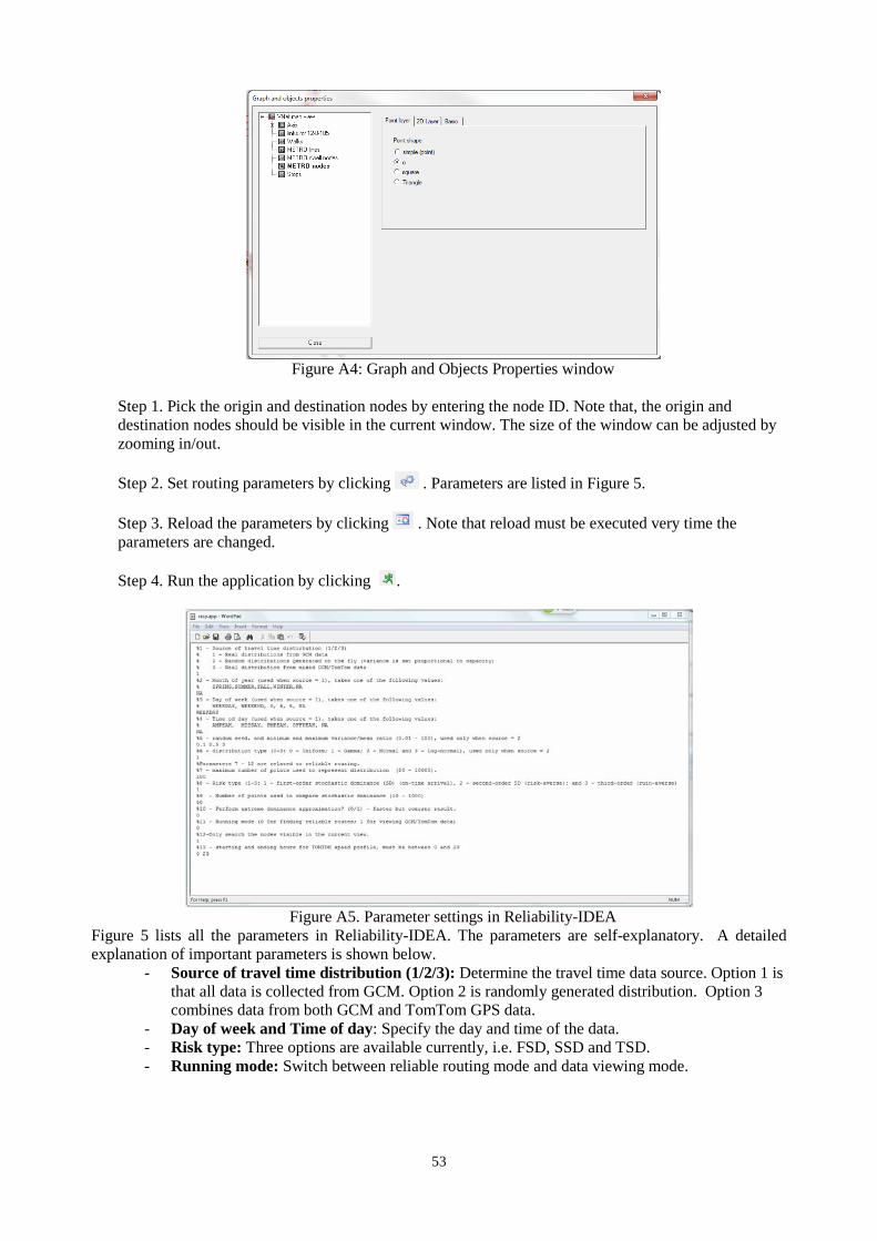
Figure A4: Graph and Objects Properties window

Step 1. Pick the origin and destination nodes by entering the node ID. Note that, the origin and destination nodes should be visible in the current window. The size of the window can be adjusted by zooming in/out. Step 2. Set routing parameters by clicking . Parameters are listed in Figure 5. Step 3. Reload the parameters by clicking . Note that reload must be executed very time the parameters are changed. Step 4. Run the application by clicking .

Figure A5. Parameter settings in Reliability-IDEA

Figure 5 lists all the parameters in Reliability-IDEA. The parameters are self-explanatory. A detailed explanation of important parameters is shown below.

- Source of travel time distribution (1/2/3): Determine the travel time data source. Option 1 is that all data is collected from GCM. Option 2 is randomly generated distribution. Option 3 combines data from both GCM and TomTom GPS data.

- Day of week and Time of day: Specify the day and time of the data. - Risk type: Three options are available currently, i.e. FSD, SSD and TSD. - Running mode: Switch between reliable routing mode and data viewing mode.

53

Figure A6. Returned routes in Reliability-IDEA

Once parameters are set properly, VNET returns possible routes as shown in Figure A6. At this stage, post operations are available and explained as follows.

- View/save reliable paths: Save reliable paths to inventory for future reference. - View/Delete saved reliable paths: View/Delete saved reliable paths. - Export/Import saved reliable paths: Export/Import reliable paths to/from .txt files. - View link distributions: Display CDF and PDF of selected link. Figure A7 shows a link

distribution comparison between GCM and TomTom data. - View TomTom speed profile: Display GCM and TomTom speed profile over time, see Figure A8. - View TomTom route reports: Display the comparison between GCM and TomTom route CDF.

Figure A7. Link distribution comparison in GCM and

TomTom

54

Figure A8. Speed profile over time

55

REFERENCES

(1) Y. Iida and H Wakabayashi. An approximation method of terminal reliability of road network using partial minimal path and cut set. In Proceedings of the Fifth World Conference, vol. IV, pages 367–380, Yokohama, Japan, 1989. (2) Z. P. Du and A. Nicholson. Degradable transportation systems: sensitivity and reliability analysis. Transportation Research Part B, 31:225–237, 1997. (3) Y. Asakura, E. Hato, and M. Kashiwadani. OD matrices estimation model using AVI data and its application to the han-shin expressway network. Transportation, 27:419–438, 2000. (4) A. Chen, H. Yang, H. Lo, and W.H. Tang. A capacity related reliability for transportation networks. Journal of Advanced Transportation, 33(2):183–200, 1999. (5) A. Chen, H. Yang, H. Lo, and W.H. Tang. Capacity reliability of a road network: an assessment methodology and numerical results. Transportation Research Part B, 36:225–252, 2002. (6) Y. Nie and X. Wu. Shortest path problem considering on-time arrival probability. Transportation Research Part B, 43(6):597–613, 2009. (7) Hong K. Lo, X. W. Luo, and Barbara W. Y. Siu. Degradable transport network: travel time budget of travelers with heterogeneous risk aversion. Transportation Research Part B, 40(9):792–806, 2006. (8) Y. Nie. Multi-class percentile user equilibrium with flow-dependent stochasticity. Transportation Research Part B, 45:1641–1659, 2011. (9) R. W. Hall. The fastest path through a network with random time-dependent travel time. Transportation Science, 20(3):182–188, 1986. (10) G. H. Polychronopoulos and J. N. Tsitsiklis. Stochastic shortest path problems with recourse. Networks, 27(2):133–143, 1996. (11) L. Fu and L. R. Rilett. Expected shortest paths in dynamic and stochastic traffic networks. Transportation Research Part B, 32(7):499–516, 1998. (12) R. K. Cheung. Iterative methods for dynamic stochastic shortest path problems. Naval Research Logistics, 45(8):769–789, 1998. (13) E. D. Miller-Hooks and H. S. Mahmassani. Least expected time paths in stochastic, time-varying transportation networks. Transportation Science, 34(2):198–215, 2000. (14) E. D. Miller-Hooks. Adaptive least-expected time paths in stochastic, time-varying transportation and data networks. Networks, 37(1):35–52, 2001. (15) L. Fu. An adaptive routing algorithm for in-vehicle route guidance systems with real-time information. Transportation Research Part B, 35(8):749–765, 2001. (16) S. T. Waller and A. K. Ziliaskopoulos. On the online shortest path problem with limited arc cost dependencies. Networks, 40(4):216–227, 2002. (17) J. S. Provan. A polynomial-time algorithm to find shortest paths with recourse. Networks, 41(2):115–125, 2003. (18) S. Gao and I. Chabini. Optimal routing policy problems in stochastic time-dependent networks. Transportation Research Part B, 40(2):93–122, 2006. (19) Y. Fan, R. Kalaba, and J. Moore. Shortest paths in stochastic networks with correlated link costs. Computers and Mathematics with Applications, 49(9-10):1549–1564, 2005. (20) J. L. Bander and C. C. White. A heuristic search approach for a nonstationary stochastic shortest path problem with terminal cost. Transportation Science, 36(2):218–230, 2002. (21) Y. Fan, R. Kalaba, and J. Moore. Arriving on time. Journal of Optimization Theory and Applications, 127(3):497–513, 2005. (22) H. Frank. Shortest paths in probabilistic graphs. Operations Research, 17(4):583–599, 1969. (23) C. E. Sigal, A. Alan, B. Pritsker, and J. J. Solberg. The stochastic shortest route problem. Operations Research, 28(5):1122–1129, 1980. (24) R. P. Loui. Optimal paths in graphs with stochastic or multidimensional weights. Communications of the ACM, 26(9):670–676, 1983. (25) R. Sivakumar and R. Batta. The variance-constrained shortest path problem. Transportation Science, 28(4):309–316, 1994. (26) G. Yu and J. Yang. On the robust shortest path problem. Computers and Operations Research, 25(6):457–468, 1998. (27) R. Montemanni and L. Gambardella. An exact algorithm for the robust shortest path problem with interval data. Computers and Operations Research, 31(10):1667–1680, 2004.

56

(28) J.F. Bard and J.E. Bennett. Arc reduction and path preference in stochastic acyclic networks. Management Science, 37(2):198–215, 1991. (29) E. Miller-Hooks. Optimal Routing in Time-Varying, Stochastic Networks: Algorithms and Implementations. PhD thesis, Department of Civil Engineering, University of Texas at Austin, 1997. (30) E. D. Miller-Hooks and H. S. Mahmassani. Path comparisons for a priori and time-adaptive decisions in stochastic, time-varying networks. European Journal of Operational Research, 146(2):67–82, 2003. (31) E. Miller-Hooks and H. Mahmassani. Optimal routing of hazardous materials in stochastic, time-varying transportation networks. Transportation Research Record, 1645:143–151, 1998. (32) Yu Nie, Xing Wu, John F. Dillenburg, and Peter C. Nelson. Reliable route guidance: A case study from Chicago. Transportation Research Part A, 46(2):403–419, 2012. (33) Xing Wu and Yu Nie. Modeling heterogeneous risk-taking behavior in route choice: A stochastic dominance approach. Transportation Research Part A, 45(9):896–915, 2011. (34) M. Friedman and L.P. Savage. The utility analysis of choices involving risk. Journal of Political Economy, 56:279–304, 1948. (35) V. S. Bawa. Optimal rules for ordering uncertian prospects. Financial Economics, 2:95–121, 1975. (36) Daniel D. Heyer. Stochastic dominance: a tool for evaluating reinsurance alternatives. In Casualty Actuarial Society Forum, 2001. (37) Christian Ullrich. Forecasting and Hedging in the Foreign Exchange Markets, chapter Preferences over Probability Distributions, pages 117–131. Springer Berlin Heidelberg, 2009. (38) Y. Nie, X. Wu, P. Nelson, and J. Dillenburg. Providing reliable route guidance using Chicago data. Technical Report 2009-001 1, Center for the Commercialization of the Innovative Transportation Technology, Northwestern University, Evanston, IL, 2009. (39) Abishai Polus. A study of travel time and reliability on arterial routes. Transportation, 8(2):141–151, 1979.

57