Urban growth patterns and growth managementboundaries in the Central Puget Sound,Washington, 1986–2007

Jeffrey Hepinstall-Cymerman & Stephan Coe &

Lucy R. Hutyra

# Springer Science+Business Media, LLC 2011

Abstract Many regions of the globe are experiencing rapid urban growth, the locationand intensity of which can have negative effects on ecological and social systems. Insome locales, planners and policy makers have used urban growth boundaries to directthe location and intensity of development; however the empirical evidence for theefficacy of such policies is mixed. Monitoring the location of urban growth is anessential first step in understanding how the system has changed over time. Inaddition, if regulations purporting to direct urban growth to specific locales arepresent, it is important to evaluate if the desired pattern (or change in pattern) hasbeen observed. In this paper, we document land cover and change across six dates(1986, 1991, 1995, 1999, 2002, and 2007) for six counties in the Central PugetSound, Washington State, USA. We explore patterns of change by three differentspatial partitions (the region, each county, 2000 U.S. Census Tracks), and with respectto urban growth boundaries implemented in the late 1990’s as part of the state’sGrowth Management Act. Urban land cover increased from 8 to 19% of the studyarea between 1986 and 2007, while lowland deciduous and mixed forests decreasedfrom 21 to 13% and grass and agriculture decreased from 11 to 8%. Land in urbanclasses outside of the urban growth boundaries increased more rapidly (by area andpercentage of new urban land cover) than land within the urban growth boundaries,suggesting that the intended effect of the Growth Management Act to direct growth towithin the urban growth boundaries may not have been accomplished by 2007. Urbansprawl, as estimated by the area of land per capita, increased overall within the

Urban EcosystDOI 10.1007/s11252-011-0206-3

J. Hepinstall-Cymerman (*)Warnell School of Forestry & Natural Resources, University of Georgia, Athens, GA 30206-2152, USAe-mail: jhepinstall@warnell.uga.eduURL: www.warnell.uga.edu

S. CoePuget Sound Regional Council, 1011 Western Ave, #500, Seattle, WA 98104-1035, USA

L. R. HutyraDepartment of Geography & Environment, Boston University, 675 Commonwealth Ave, Boston, MA02215, USA

region, with the more rural counties within commuting distance to cities having thehighest rate of increase observed. Land cover data is increasingly available and can beused to rapidly evaluate urban development patterns over large areas. Such data areimportant inputs for policy makers, urban planners, and modelers alike to manage andplan for future population, land use, and land cover changes.

Keywords Land cover change . Spatial patterns . Urban growth . Urban growth boundary.

Growth management . Urban-rural interface . Sprawl

Introduction

Urbanization, the conversion of lands that were previously undeveloped or in low densityand low intensity forms of development (e.g., rural areas, agricultural lands) to urban landcover, is occurring at a rapid pace throughout the world (Houghton 1994) and the U.S. inparticular (Brown et al. 2005). The land area that is urbanized continues to increase as thehuman population grows (Alberti et al. 2003; Grimm et al. 2000; Houghton 1994; Meyerand Turner 1992), with approximately 3% of Earth’s land area currently in urban land cover(Imhoff et al. 2004). Urban growth and associated land use and land cover change havenumerous effects on ecological and social systems (Foley et al. 2005). Urbanizationchanges and often substitutes natural ecosystem processes (i.e., surface water runoff,ground water recharge, nitrogen balances, light availability) with human constructedinfrastructure (e.g., sewer systems and wastewater treatment plants).

Ecosystems are often degraded with urbanization. Documenting and monitoring landcover change over time is essential for understanding both system trends and the specificchanges that have occurred (Ji et al. 2006). As areas become developed and land useschange from primarily production agriculture and forestry to residential, commercial, andindustrial uses, the land cover of these areas change significantly both in speciescomposition (e.g., from forest stands to non-native shrubs, lawn, and planted tree specieswith remnant patches of native forest) and in structure with more impervious surface areaand simplified vertical diversity of vegetation (Robinson et al. 2005). The conversion oflarge areas of agricultural and forested lands, which hold great stores of biodiversity (Foleyet al. 2005), into developed land cover has potential impact on the native biodiversity of anarea (Hansen et al. 2001; Hepinstall et al. 2009; Pearson et al. 1999). Characterizing landcover of urban and urbanizing areas and change over time are important to several fieldsincluding urban ecology and urban planning (Alberti et al. 2003; Powell et al. 2008;Robinson et al. 2005; Yang et al. 2003), land cover change modeling (Hepinstall et al. 2008)and landscape ecology (Hobbs and Wu 2007).

Documenting patterns of urban development is also important to urban and regionalplanners who are interested in directing growth to be more efficient with the co-location ofinfrastructure and public services with residential areas thereby reducing transportationcosts with concomitant reductions in greenhouse gas emissions. Land use regulations (e.g.,zoning and building codes) can also be used to direct urbanization in ways that have fewernegative impacts on biological systems by, for example, slowing the conversion ofproductive agricultural lands or forests to development. Low-density, dispersed, and leap-frog development, often labeled “urban sprawl” (Kunstler 1994) at the edges of existingmetropolitan areas or “rural sprawl” (Radeloff et al. 2005) in rural areas has been a commondevelopment pattern throughout the U.S. (Theobald 2001), Canada, Japan, and portions ofEurope (Millward 2006).

Urban Ecosyst

One method for mitigating urban growth patterns that are perceived as negative (i.e.,sprawl) is through planning and the institution of development boundaries such as urbangrowth boundaries (UGB) beyond which urban development is discouraged and withinwhich planned growth is encouraged (Millward 2006). UGB are development boundarieswith accompanying regulations set up by local municipalities designed to focus high-density urban development inside and conserve rural and undeveloped lands outside of theboundaries. The boundaries are specifically delineated to provide enough developable landto accommodate the projected growth in population for the region ~20 years into the future(Cho et al. 2008). Planned growth or “smart growth” includes many ideas including: mixedland uses with compact building design; walkable communities; and preservation of openspace, agricultural lands, and critical environmental areas (Tregoning et al. 2002). Severalstudies have concluded that in theory, UGB would lead to economically efficient anti-sprawl solutions (Bento et al. 2006) and increase social welfare by managing growth andcoordinating with infrastructure investment cycles (Ding et al. 1999).

These “strong control” planning techniques have been implemented in many localesincluding Portland, Oregon (Harvey and Works 2002), Vancouver, British Columbia (Tomalty2002), and Washington State since sprawl was recognized as a potential problem in the U.S.in the early 1970’s (Real Estate Research Corp 1974). Different levels of control of urbangrowth are available depending on the goals of the growth management legislation (Millward2006), but generally there are areas where urban development is promoted with areas beyondthese boundaries being designated as “open space” or a “green belt” of undeveloped lands.

The empirical evidence for UGB actually slowing sprawling development is mixed withstudies indicating slowed growth (Gosnell et al. 2011; Kline 2005; Kline and Alig 1999;Nelson and Moore 1993), mixed results depending on location within urban or suburbanareas (Cho et al. 2008), or negative “spillover” effects of pushing development across stateborders (Jun and Hur 2001). Portland, Oregon was an early adopter of UGB in the U.S.,passing legislation to direct the location of growth in 1973. In an evaluation of the numberof residential building permits and land subdivisions between 1985 and 1989, it was clearthe UGB were having the desired effect with over 90% of permits and 98.8% ofsubdivisions located within the UGB (Nelson and Moore 1993). Analysis of the effects ofPortland’s 1979 UGB, which was created primarily to contain urban growth and protectagricultural and forest lands from urban development, reveals that even with this strictboundary, many large-lot (low density) parcels were built for non-agricultural uses since theenforcement of the boundary in 1985 (Harvey and Works 2002) and often these occurred onthe fringe of existing development, likely impeding future expansion of the UGB aspopulations continue to increase (Nelson and Moore 1993). Another study in EasternTennessee found that development was encouraged both within the UGB in already urbanareas and outside of the UGB on the rural-urban margin (Cho et al. 2008).

It is possible to use geospatial data (i.e., land cover, land use, census data on population,housing density) to explore the spatial patterns of development. For example, Radeloff et al.(2005) explored the spatial pattern of housing growth across the U.S. from 1940 to 2000using U.S. Census data and combined these data with a land cover map to determine bothwhere housing growth at different densities occurred and how that related to the currentextent of forests (i.e., potential stores of biodiversity). From this work the authors were ableto document that increased housing density had occurred both along metropolitan fringes(urban sprawl) and in non-metropolitan areas (rural sprawl). However, this approach doesnot allow one to conclude why these patterns have occurred or to directly attribute them toland use planning efforts (Gosnell et al. 2011), but they do provide important informationregarding observed change in land use/land cover.

Urban Ecosyst

Land cover maps derived from satellite-based remote sensing are increasingly availableand provide a ready source of medium-resolution imagery (e.g., Landsat Thematic Mappervisible and infra-red sensors record data at 30-m resolution) from which to map land coverchanges across time. Several recent studies have used remote sensing, land cover maps,and/or spatial pattern metrics to document temporal changes in urban extent and pattern(Boentje and Blinnikov 2007; Chen et al. 2000; Epstein et al. 2002; Herold et al. 2005; Ji etal. 2001; Lo and Yang 2002; Sudhira et al. 2004; Sutton 2003; Yang and Lo 2002; Yuan etal. 2005). Herold et al. (2003) provide a review of spatial metrics and methods used tomeasure urban land cover using remotely sensed imagery.

The objective of our study was to identify spatial patterns of land cover over time bydifferent political jurisdictions and growth management policies. Specifically, we comparedtemporal changes in composition and configuration of land cover at three spatial scales: 1) asix county region in of the Central Puget Sound; 2) by individual counties; and 3) by censustracts. We also compared changes with respect to Urban Growth Boundaries designated aspart of the 1990 Growth Management Act and implemented by counties and cities throughcomprehensive plans developed in the mid 1990s through the early 2000’s. Finally, wecompared land cover change with population estimates and calculated a per-capitaconsumption of land over time as one of many possible metrics describing sprawl.

Similar to Ji et al. (2006), we believe that it is important to conduct analyses at scalesrelevant to local and regional jurisdictions where decisions regarding planning anddevelopment options occur. At the regional level, the Puget Sound Regional Council is aregional planning agency (and designated Metropolitan Planning Organization for theregion) currently composed of representatives from four counties (King, Kitsap, Pierce, andSnohomish) and cities, towns, ports, tribes, transit agencies, and the state government.While not generally a spatial unit used in planning, we conducted analysis for each censustrack as our finest resolution analysis primarily to develop a digital database that will beuseful to other researchers since there is a wealth of information resulting from U.S.Censuses. We were specifically interested in how land cover patterns changed over time andspace and whether there were any discernible patterns that could be attributed to urbangrowth boundaries implemented in the late 1990’s and early 2000’s.

Evaluating the effectiveness of UGB is difficult since myriad processes are present in anurban and urbanizing region and it is difficult to attribute any one observed pattern to aspecific policy. However, in theory, if designated UGB provide adequate buildable land andfocus new growth within their boundaries, then several hypotheses can be postulatedconcerning the location and intensity of new growth: 1) greater development by area and bypercentage of new development observed in one time period will have occurred within theboundaries; and 2) discrete patches of new development in each time period will be largerinside rather than outside of the UGB. While we do not attempt to directly evaluate theeffectiveness of the UGB at directing new urban development, these hypotheses concerningthe location and configuration of new development can be tested using increasinglyavailable land use and land cover (LULC) data. Landsat Thematic Mapper satellite imagerywhich can be processed into land cover maps is now freely available, likely stimulating theproduction of additional LULC maps.

Study area

The study area is approximately 17,700 km2 of land area encompassing the Central PugetSound of western Washington, USA, (Fig. 1) and includes all or portions of six counties

Urban Ecosyst

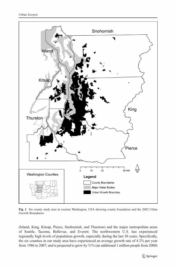
(Island, King, Kitsap, Pierce, Snohomish, and Thurston) and the major metropolitan areasof Seattle, Tacoma, Bellevue, and Everett. The northwestern U.S. has experiencedregionally high levels of population growth, especially during the last 30 years. Specifically,the six counties in our study area have experienced an average growth rate of 4.2% per yearfrom 1986 to 2007; and is projected to grow by 31% (an additional 1 million people from 2000)

Fig. 1 Six county study area in western Washington, USA showing county boundaries and the 2002 UrbanGrowth Boundaries

Urban Ecosyst

by 2025 (Office of Financial Management, State of Washington: http://www.ofm.wa.gov/pop/accessed 16 May 2010).

In 1990 the state of Washington legislature passed the “Growth Management Act”(GMA; “Growth management–planning by selected counties and cities”, RCW 36.70A),which mandated the use of comprehensive land use planning with the goal of preventingunplanned and haphazard land development—the type of growth that typically results indispersed development patterns and highly fragmented exurban development and is oftenlabeled as sprawl or urban sprawl. Counties of a certain size and growth rate (>50,000inhabitants with >10% in previous 10 years or counties with any population size and >20%growth rate) and the cities within them are required to develop comprehensive plans anddevelopment regulations guided by 14 goals covering various social, economic, andenvironmental elements. Section 36.70A.110 sets forth the designation of urban growthareas in comprehensive plans by setting boundaries within which growth is encouraged andoutside of which growth “can only occur if it is not urban in nature”. The Act does notexplicitly define “not urban in nature”, but it can be understood as single-family residentialon lots larger than ~0.5 acres. By October 1, 1993, the counties that met the growth criteriarequiring them to follow RCW 36.70A were expected to have provisional urban growthareas designated. Four of the six counties in our study area (King, Kitsap, Pierce, andSnohomish) began in 1993 to develop comprehensive plans in compliance with the GMA.By 1994 King County had adopted a comprehensive plan that designated urban growthareas and the four counties had formed the Puget Sound Regional Council through whichthe VISION 2020 document was developed that outlined regional planning policies thatwere in compliance with the GMA. Pierce, Thurston, and Snohomish Counties followedwith comprehensive plans enacted in 1995; Kitsap and Island Counties in 1998.

The GMA uses state funding of public works to encourage jurisdictional compliance,stating that, “only those jurisdictions in compliance with the review and revision schedulesof the growth management act are eligible to receive funds from the public works assistanceand water quality accounts in the state treasury” (36.70A.130 Notes: Intent 2005c294).However, many jurisdictions did not comply with original and subsequently reviseddeadlines, so that by 2005 the act was amended to allow jurisdictions making significantprogress towards compliance to be granted an additional 12 months of eligibility for funds(36.70A.130 Notes: Intent 2005c294). Because of the difficulty in determining the exactgrowth management boundaries for each jurisdiction and when each was enacted andenforced, we used a spatial database containing GMA boundaries available statewide withan effective date of 2002 when making comparisons of growth inside and outside ofdesignated urban growth boundaries.

Methods

Land cover data

We used 14-class land cover data for 1986, 1991, 1995, 1999, 2002, and 2007 developed from acombination of Landsat Thematic Mapper (TM) and Enhanced TM (ETM+) imagery(Hepinstall-Cymerman et al. 2009). Multiple methods were used to differentiate 14 landcover classes in each image. Supervised and unsupervised classifications were combined withspectral unmixing techniques on multi-season imagery for each date. Differences betweenleaf-on (June-July) and leaf-off images (March–April) were used to differentiate between landcover classes spectrally similar in one season and dissimilar in another (e.g., deciduous versus

Urban Ecosyst

coniferous forest, agriculture versus low-density urban). Multi-season data has beensuccessfully used in the past (Lunetta and Balogh 1999; Oetter et al. 2001) to differentiateland cover classes that may be spectrally similar in one season and dissimilar in another. Inaddition, the surface heterogeneity of urban areas leads to spectrally heterogeneous imagery atsmall spatial scales. Spectral unmixing of the leaf-on imagery was used to separate heavyurban (80–100% impervious area), medium urban (50–80% impervious), and light urban (20–50% impervious). The level of impervious area is an important determinant of manyecosystem processes (Lu and Weng 2006; Tang et al. 2005). Landscape trajectories, ortemporal patterns of land cover change, were used to correct for classification errors betweendates so that urban areas either stayed at the same level of imperviousness or became moreimpervious over time. Several land cover classes were derived from ancillary GIS layers(open water, non-forested wetland, shorelines, and ice/snow fields); we did not consider theseclasses in this study since they are constant throughout the land cover maps.

Comparing land cover composition and configuration over time and space

Land cover maps for each date were compared pixel-by-pixel to determine land coverchange during our study period (1986–2007). We calculated landscape composition (areaand percentage) and patch-based landscape composition metrics for three spatial strata: 1)the six county study area; 2) for each county by date; and 3) by U.S. census tract (2000)boundaries. We also calculated change between subsequent dates for each spatial stratum.Additionally, we calculated the same metrics separately for those areas inside (i.e., urbangrowth areas) and outside of the 2002 UGB (obtained from the State of WashingtonDepartment of Ecology) for each date and stratum. We calculated the area and percentage ofnew urban (pixels that were not an urban class in the previous time period but subsequentlybecame urban) for 1991–2007. We used Fragstats 3.3 (McGarigal et al. 2002) to calculatepatch-based “landscape metrics” or more broadly “spatial metrics” (Herold et al. 2003)measuring landscape configuration for all urban classes combined (Heavy, Medium, Light,Cleared for Development; Table 1). We selected metrics based on previous studies (Albertiet al. 2007; Hepinstall et al. 2008, 2009; Herold et al. 2003; Ji et al. 2006) and included

Table 1 Land cover classes used in this study

Final classification Abbreviation Class definition

Heavy intensity urban HIU >80% Impervious Area

Medium intensity urban MIU 50–80% Impervious Area

Light intensity urban & landcleared for development

LIU 20–50% Impervious Area class combined with Land thatwas vegetated in a previous time step and urban in alater time step

Grass GR Developed Grass and Grasslands

Agriculture AG Row Crops, Pastures

Deciduous and mixed forest DMF >80% Deciduous Trees, 10–80% each Decid./Conif. Trees

Coniferous forest CF >80% Coniferous Trees

Clearcut forest & regeneratingforest

CC & REG Clearcut Forest and Re-growing Forest combined

Other Other Water, Non-forested Wetlands, Shoreline (tidal areas bareduring low tide), and Snow/Ice/Bare Rock (high elevationareas with no vegetation or snow cover) combined

Urban Ecosyst

metrics that measure the amount of edge, the shape of patches, and aggregation of patches.Specifically, we calculated the following metrics for individual classes: number of patchesper unit area (PD) using 8-way neighbors to define patches; the amount of edge per unitarea (ED); shape of patches (LSI); and aggregation index (AI) which measures how oftenpixels are contiguous to pixels of the same class scaled from 1 to 100 (McGarigal et al.2002). In addition to the class-based landscape metrics, we calculated two metrics thatmeasured patterns across all 14 land cover classes at once (i.e., “landscape metrics” inFragstats) as an indication landscape patterns integrating all mapped classes: Shannon’sDiversity Index (SHDI) which measures the number of different land cover classes present;and Shannon’s Evenness Index (SHEI) which measures how evenly distributed (by area)the existing land cover classes are across the study area. In urbanizing rural or forestedlandscapes, SHDI will increase and SHEI will decrease; urbanizing suburban landscapeswill experience the opposite trend.

Measures of urban sprawl

To understand how increased urban land cover tracked with population (e.g., percapita land consumption), we calculated an annualized urban sprawl index (AUSI) asthe area (km2) of new urban land cover divided by the population change (in thousands)for the same time period (person per 0.10 ha), each annualized by the number of yearsrepresented. While there are many different measures of “sprawl” available, most requirefine-scaled data on specific landscape elements (e.g., number of cul-de-sacs, sidewalks)that were not available for our study area. Our AUSI metric is similar to the urban sprawlindex in Yuan et al. (2005) where we have annualized change to be able to compare acrossmultiple time periods. Population data by county were downloaded from the WashingtonState Office of Financial Management (http://www.ofm.wa.gov/pop accessed on 4 July2007 and 16 May 2010) and represent yearly estimates of the number of residents in eachcounty.

Results

Land cover composition

Between 1986 and 2007 urban areas spread out from the existing urban core cities ofSeattle, Bellevue, Tacoma, Olympia, Everett, and Bremerton, into the lower elevationsand up canyons. The area of land in urban classes has steadily increased at the sametime that grass, agriculture, and forested classes were decreasing (Table 2). Urban areaswere primarily converted from grass, agriculture, and deciduous and mixed forest. Someof these patterns are driven by changes in the yearly extent of snow when the images wereacquired and problems with classifying high elevation conifer that still had snow on theground. For example, the large differences between 2007 and 2002 in grass andconiferous forest are driven primarily by differences at high elevations and are likely dueto discrepancy in the land cover maps rather than actual land cover changes on the ground(not shown).

When comparing the total area of each class across time within and outside of the UGBwe observed that urban land cover increased from 1,167 km2 in 1986 to 1,936 km2 in 2007inside of the UGB, an increase of 65.9%, and representing 41.3% and 68.6% of the areainside the UGB (Table 2). Conversely, urban areas outside of the UGB, while covering less

Urban Ecosyst

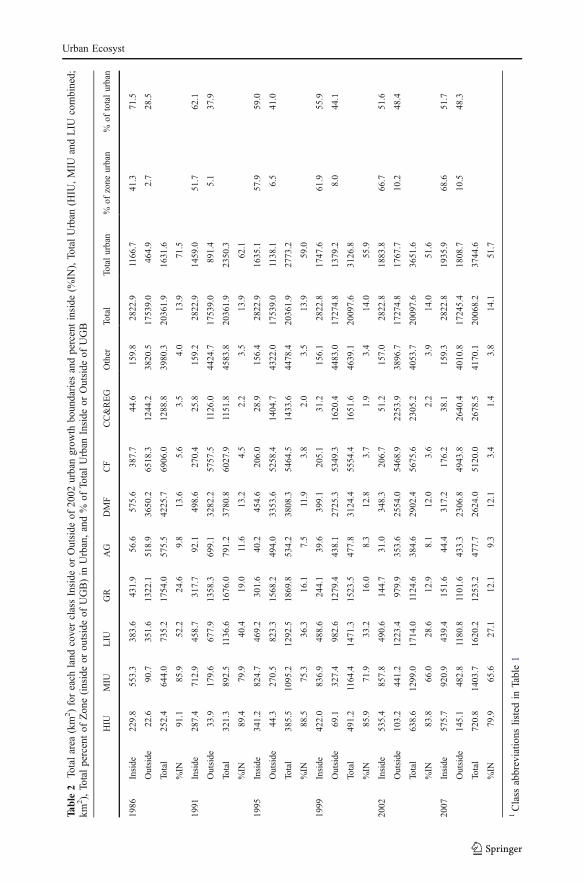
Table

2Totalarea

(km

2)foreach

land

coverclassInside

orOutside

of20

02urbangrow

thbo

undaries

andpercentinside

(%IN

),TotalUrban

(HIU

,MIU

andLIU

combined;

km2),Totalpercentof

Zon

e(insideor

outsideof

UGB)in

Urban,and%

ofTotalUrban

Inside

orOutside

ofUGB

HIU

MIU

LIU

GR

AG

DMF

CF

CC&REG

Other

Total

Totalurban

%of

zone

urban

%of

totalurban

1986

Inside

229.8

553.3

383.6

431.9

56.6

575.6

387.7

44.6

159.8

2822.9

1166.7

41.3

71.5

Outside

22.6

90.7

351.6

1322.1

518.9

3650.2

6518.3

1244.2

3820.5

17539.0

464.9

2.7

28.5

Total

252.4

644.0

735.2

1754.0

575.5

4225.7

6906.0

1288.8

3980.3

20361.9

1631.6

%IN

91.1

85.9

52.2

24.6

9.8

13.6

5.6

3.5

4.0

13.9

71.5

1991

Inside

287.4

712.9

458.7

317.7

92.1

498.6

270.4

25.8

159.2

2822.9

1459.0

51.7

62.1

Outside

33.9

179.6

677.9

1358.3

699.1

3282.2

5757.5

1126.0

4424.7

17539.0

891.4

5.1

37.9

Total

321.3

892.5

1136.6

1676.0

791.2

3780.8

6027.9

1151.8

4583.8

20361.9

2350.3

%IN

89.4

79.9

40.4

19.0

11.6

13.2

4.5

2.2

3.5

13.9

62.1

1995

Inside

341.2

824.7

469.2

301.6

40.2

454.6

206.0

28.9

156.4

2822.9

1635.1

57.9

59.0

Outside

44.3

270.5

823.3

1568.2

494.0

3353.6

5258.4

1404.7

4322.0

17539.0

1138.1

6.5

41.0

Total

385.5

1095.2

1292.5

1869.8

534.2

3808.3

5464.5

1433.6

4478.4

20361.9

2773.2

%IN

88.5

75.3

36.3

16.1

7.5

11.9

3.8

2.0

3.5

13.9

59.0

1999

Inside

422.0

836.9

488.6

244.1

39.6

399.1

205.1

31.2

156.1

2822.8

1747.6

61.9

55.9

Outside

69.1

327.4

982.6

1279.4

438.1

2725.3

5349.3

1620.4

4483.0

17274.8

1379.2

8.0

44.1

Total

491.2

1164.4

1471.3

1523.5

477.8

3124.4

5554.4

1651.6

4639.1

20097.6

3126.8

%IN

85.9

71.9

33.2

16.0

8.3

12.8

3.7

1.9

3.4

14.0

55.9

2002

Inside

535.4

857.8

490.6

144.7

31.0

348.3

206.7

51.2

157.0

2822.8

1883.8

66.7

51.6

Outside

103.2

441.2

1223.4

979.9

353.6

2554.0

5468.9

2253.9

3896.7

17274.8

1767.7

10.2

48.4

Total

638.6

1299.0

1714.0

1124.6

384.6

2902.4

5675.6

2305.2

4053.7

20097.6

3651.6

%IN

83.8

66.0

28.6

12.9

8.1

12.0

3.6

2.2

3.9

14.0

51.6

2007

Inside

575.7

920.9

439.4

151.6

44.4

317.2

176.2

38.1

159.3

2822.8

1935.9

68.6

51.7

Outside

145.1

482.8

1180.8

1101.6

433.3

2306.8

4943.8

2640.4

4010.8

17245.4

1808.7

10.5

48.3

Total

720.8

1403.7

1620.2

1253.2

477.7

2624.0

5120.0

2678.5

4170.1

20068.2

3744.6

%IN

79.9

65.6

27.1

12.1

9.3

12.1

3.4

1.4

3.8

14.1

51.7

1Class

abbreviatio

nslistedin

Table1

Urban Ecosyst

area in 1986 (465 km2) increased 289% by 2007 to 1,809 km2 (from 2.7% to 10.5% of thezone including unbuildable lands in the Cascade Mountains). Between 1986 and 2002inside the UGB, heavy and medium intensity urban classes increased (151% and 66%,respectively) more than light intensity urban (15%). Outside of the UGB the pattern wassimilar but the percentage change was much larger (HIU: 542%; MIU 432%; LIU 236%increase). The percentage of each urban class that was inside the UGB steadily decreased atthe same time the total area of urban land was increasing across the region; by 2007 thecombined area for all urban classes for our study area indicated the nearly 50% of all urbanland was located outside of the UGB. The increase in urban land cover came at the expenseof Grass, Deciduous and Mixed Forest, and Coniferous Forest which all decreased in totalarea and in the percentage within the UGB.

Because the Growth Management Act was passed in the early 1990’s, but notimplemented until after 1995 or 1998, depending on the county in our study area, wecompared annualized rates of increase in urban land cover across time to see if we coulddetect any patterns potentially attributable to the passage of comprehensive plans by eachjurisdiction. More land area was being converted to urban classes outside of the UGB thaninside the UGB across all dates with the greatest disparity in development occurringbetween 1999 and 2002 when we observed almost three times as much new urban landoutside the UGB as inside (Fig. 2). The annualized rates (Fig. 2 numbers within bars) showa large increase in both the total amount of new urban and the amount occurring outside ofthe UGB between 1999 and 2002.

Visualizing the patterns of change in urban land cover with respect to the UGB isdifficult given our large study area, the fine grain data, and the highly heterogeneouslandscape. To highlight changes, we selected only those areas that changed into an urbanclass from a non-urban class in the previous date and then compared the distribution ofthese areas of new urban inside and outside of the UGB. New urban areas werepredominately outside of the UGB, with 2002 representing the lowest percentage of newdevelopment occurring within the UGB; even while the amount of new urban increasedsubstantially from the 1995 to 1999 time period (Fig. 2). We have included a figuremapping the patterns of new urban in 1999, 2002, and 2007 with respect to existing urbanas of 1995 and the UGB for a small but representative section of King and Snohomishcounties including northern Seattle and Bellevue (Fig. 3). While a large portion of the

Fig. 2 New urban land coverdistribution (% of total newurban since last date of landcover) inside or outside of 2002Urban Growth Boundaries byyear. Numbers in bars indicatethe annualized area (km2) of newurban added inside or outside ofthe UGB since the previous date

Urban Ecosyst

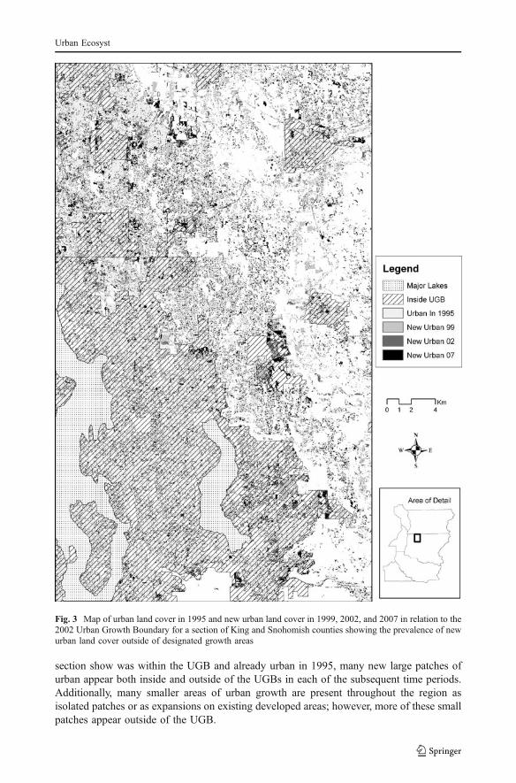
section show was within the UGB and already urban in 1995, many new large patches ofurban appear both inside and outside of the UGBs in each of the subsequent time periods.Additionally, many smaller areas of urban growth are present throughout the region asisolated patches or as expansions on existing developed areas; however, more of these smallpatches appear outside of the UGB.

Fig. 3 Map of urban land cover in 1995 and new urban land cover in 1999, 2002, and 2007 in relation to the2002 Urban Growth Boundary for a section of King and Snohomish counties showing the prevalence of newurban land cover outside of designated growth areas

Urban Ecosyst

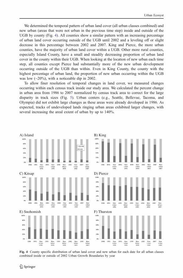
We determined the temporal pattern of urban land cover (all urban classes combined) andnew urban (areas that were not urban in the previous time step) inside and outside of theUGB by county (Fig. 4). All counties show a similar pattern with an increasing percentageof urban land cover occurring outside of the UGB until 2002 and a leveling off or slightdecrease in this percentage between 2002 and 2007. King and Pierce, the more urbancounties, have the majority of urban land cover within a UGB. Other more rural counties,especially Island County, have a small and steadily decreasing proportion of urban landcover in the county within their UGB. When looking at the location of new urban each timestep, all counties except Pierce had substantially more of the new urban developmentoccurring outside of the UGB than within. Even in King County, the county with thehighest percentage of urban land, the proportion of new urban occurring within the UGBwas low (~20%), with a noticeable dip in 2002.

To allow finer resolution of temporal changes in land cover, we measured changesoccurring within each census track inside our study area. We calculated the percent changein urban area from 1986 to 2007 normalized by census track area to correct for the largedisparity in track sizes (Fig. 5). Urban centers (e.g., Seattle, Bellevue, Tacoma, andOlympia) did not exhibit large changes as these areas were already developed in 1986. Asexpected, tracks of undeveloped lands ringing urban areas exhibited larger changes, withseveral increasing the areal extent of urban by up to 140%.

A) Island B) King

C) Kitsap D) Pierce

E) Snohomish F) Thurston

Fig. 4 County specific distribution of urban land cover and new urban for each date for all urban classescombined inside or outside of 2002 Urban Growth Boundaries by year

Urban Ecosyst

Land cover configuration

A previous study looked at changes in the patterns of landscape composition andconfiguration for this region from 1986 to 2002 using simple landscape metrics (Hepinstall-Cymerman et al. 2009). We extended this by including 2007 data and looking at moremetrics over different politically defined spatial partitions (county and census track). Here

Fig. 5 Map of change in urban amount in each census track from 1986 to 2007 normalized by census track area

Urban Ecosyst

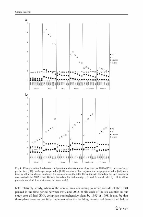
we focus on six metrics calculated for all urban classes combined. Within in the UGB from1986 to 2007, as the area of urban classes (CA) increased across all time periods (Table 2),LSI, ED, PD were decreasing and AI was increasing—all trends indicating that the overallpattern of urban growth was expansion of established urban areas and infill rather than theestablishment of new patches of urban land cover (Fig. 6a). Outside of the UGB thepatterns were more variable. Both PD and LSI generally peaked in 1991, and AI steadilyincreased from 1986 to 2007, indicating that the urban areas in this region were beginningto consolidate into larger patches (Fig. 6b). Edge Density, however, was increasing for allcounties from 1986 to 2007 outside the UGB indicating that new urban areas were notalways simply expansion.

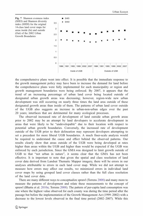
The overall composition and configuration of the landscape clearly changed during the studyperiod. Inside of the UGB, both the SHEI and SHDI decrease across all time periods indicatingthat the area inside the UGB was becoming less diverse and less even (Fig. 7). This trendmatches the increase in urban area and elimination of patches of non-urban classes depictedby county in Fig. 6a. Outside of the UGB the trend is the reverse with a steady increase inboth SHEI and SHDI over time, indicating both an increase in fragmentation (increasedevenness indicates more even distribution of patch types) and an increase in diversity of classtypes as urban classes expanded into previously undeveloped areas.

Per-capita land consumption

We compared how changes in human population have tracked changes in urban land area(Table 3). Populations increased consistently (yearly range: 800 for Island County between2002 and 2007 to 34,800 in King County between 1986 and 1991) across the six countiesin our study area. The area in urban land cover increased yearly and relatively consistentlyfor each county until the final time interval when the amount of change droppedsignificantly across all counties. Our basic annualized urban sprawl index (AUSI) indicatedthat new urban land cover was not clearly aligned with increased population across time orspace. Specifically, King, Pierce, and Snohomish counties show the highest AUSI between(1999 and 2002), and the lowest AUSI levels observed in the final time period (2002–2007).

Discussion

This six county region underwent a large increase in urban land between 1986 and 2007, atthe expense of grass, agriculture, and lowland deciduous and mixed forest. As the area ofurban land cover grew, it became more consolidated and continuous within urban growthareas, while at the same time continuing to increase in area and number of discrete patchesof new urban land cover outside of the urban growth areas. Similar patterns have beenobserved in other studies examining temporal changes in urban patterns (Ji et al. 2006;Torrens 2008)

Consistently across all dates, the percentage of new urban land that fell outside of theUGB was larger than the percentage of new urban land that fell within the UGB. The onlyexception was for Pierce County where the majority of land cover change to urban wasoccurring within the UGB for the county. Similarly, Carlson and Dierwechter (2007) foundthat the percentage of building permits in Pierce County that were located outside the UGBbetween 1991 and 2002 decreased from a high of 50% in 1993 to 23% by 2002 andattributed the change to the implementation of growth management beginning in 1995.Interestingly, between 1995 and 2007, the annual increase in urban area within the UGB

Urban Ecosyst

held relatively steady, whereas the annual area converting to urban outside of the UGBpeaked in the time period between 1999 and 2002. While each of the six counties in ourstudy area all had GMA-compliant comprehensive plans by 1995 or 1998, it may be thatthese plans were not yet fully implemented or that building permits had been issued before

0

1

2

3

4

5

6

1986

1991

1995

1999

2002

2007

1986

1991

1995

1999

2002

2007

1986

1991

1995

1999

2002

2007

1986

1991

1995

1999

2002

2007

1986

1991

1995

1999

2002

2007

1986

1991

1995

1999

2002

2007

Island King Kitsap Pierce Snohomish Thurston

PD

ED

LSI/100

AI/100

0

1

2

3

4

5

6

7

8

9

1986

1991

1995

1999

2002

2007

1986

1991

1995

1999

2002

2007

1986

1991

1995

1999

2002

2007

1986

1991

1995

1999

2002

2007

1986

1991

1995

1999

2002

2007

1986

1991

1995

1999

2002

2007

Island King Kitsap Pierce Snohomish Thurston

PD

ED

LSI/100

AI/100

a

b

Fig. 6 Changes in four land cover configuration metrics (number of patches per 100 ha [PD]; meters of edgeper hectare [ED]; landscape shape index [LSI]; number of like adjacencies—aggregation index [AI]) overtime for all urban classes combined for: a areas inside the 2002 Urban Growth Boundary for each county; bareas outside the 2002 Urban Growth Boundary for each county. (LSI and AI are divided by 100 to allowpresentation of all four metrics on the same scale)

Urban Ecosyst

the comprehensive plans went into effect. It is possible that the immediate response tothe growth management policy may have been to increase the demand for land beforethe comprehensive plans were fully implemented for each municipality or region andgrowth management boundaries were being enforced. By 2007, it appears that thetrend of an increasing percentage of urban land cover being located outside ofdesignated urban growth areas was decreasing; however, region-wide new urbandevelopment was still occurring on nearly three times the land area outside of thesedesignated growth areas than inside of them. The patterns of urban land cover outsideof the UGB also suggests an increase in urban-non-urban edges over the past20 years; interfaces that are detrimental for many ecological processes.

The observed increased rate of development of land outside urban growth areasprior to 2002 may be an attempt by land developers to accelerate development inareas that were likely to be “undevelopable” due to their location with respect topotential urban growth boundaries. Conversely, the increased rate of developmentoutside of the UGB prior to their delineation may represent developers attempting toset a precedent for more liberal UGB boundaries. A much finer-scale analysis wouldbe required to understand the cause and effect behind the observed patterns. Ourresults clearly show that areas outside of the UGB were being developed at rateshigher than areas within the UGB and higher than would be expected if the UGB wasenforced by each jurisdiction. Since the GMAwas designed to limit growth outside ofUGB to that “not urban in nature”, it seems clear that the GMA has not beeneffective. It is important to note that given the spatial and class resolution of landcover data derived from Landsat Thematic Mapper imagery, there will be errors in ouranalyses attributable to errors in each land cover map. While we did not attempt tomeasure how errors may affect our results, we minimized errors in individual landcover maps by using grouped land cover classes rather than the full class resolutionof the land cover data.

There are many different ways to conceptualize sprawl (Torrens 2008) and many more tomeasure the patterns of development and relate these measurements to the concept ofsprawl (Bhatta et al. 2010a; Torrens 2008). The pattern of per-capita land consumption wasone where the highest value observed for each county was during the time period after thepassage but before the implementation of the Growth Management Act (1999–2002) with adecrease to the lowest levels observed in the final time period (2002–2007). While this

0

0.5

1

1.5

2

2.5

3

3.5

1986 1991 1995 1999 2002 2007 1986 1991 1995 1999 2002 2007

Inside of UGB Outside of UGB

SHEI

SHDI

Fig. 7 Shannon evenness index(SHEI) and Shannon diversityindex (SHDI) for the original14-class land cover maps forareas inside (In) and outside(Out) of the 2002 UrbanGrowth Boundaries

Urban Ecosyst

Table3

Hum

anpo

pulatio

n(inthou

sand

s)andannualized

change

inthou

sands(Δ

pop/year),urbanland

coverarea

(km

2)andannualized

change

(Δkm

2/year)betweendates,

andan

annualized

urbansprawlindex(annualurbanarea

expansion/annual

populatio

nexpansion)

foreach

county

with

inthestudyarea

Pop

ulation(000)

1986

1991

Δpo

p/year

1995

Δpo

p/year

1999

Δpo

p/year

2002

Δpo

p/year

2007

Δpo

p/year

Island

5162

2.2

661.1

711.1

730.8

781.1

King

1,376

1,55

034

.81,62

518

.81,712

21.7

1,774

20.7

1,86

117

.4

Kitsap

167

197

5.9

218

5.3

230

2.8

235

1.7

245

2.0

Pierce

536

598

12.4

649

12.8

689

9.9

725

12.0

791

13.1

Snoho

mish

393

488

19.0

532

10.9

589

14.4

628

12.9

686

11.7

Thu

rston

143

168

4.9

186

4.7

203

4.2

212

3.0

238

5.1

Urban

land

cover(km

2)

1986

1991

Δkm

2/year

1995

Δkm

2/year

1999

Δkm

2/year

2002

Δkm

2/year

2007

Δkm

2/year

Island

61.1

93.9

6.6

116.7

5.7

143.1

6.6

189.2

15.4

170.3

MD1

King

679.6

874.2

38.9

979.9

26.4

1055.9

19.0

1171

.238

.412

26.0

10.9

Kitsap

111.8

188.6

15.4

228.8

10.1

258.6

7.5

323.4

21.6

329.1

1.1

Pierce

379.8

540.7

32.2

656.3

28.9

744.4

22.0

861.5

39.0

891.4

6.0

Snoho

mish

267.5

413.2

29.2

486.9

18.4

565.0

19.5

672.4

35.8

685.9

2.7

Thu

rston

131.9

238.9

21.4

300.3

15.4

361.2

15.2

439.7

26.2

442.0

0.4

Annualized

urbansprawlindex

86–91

91–95

95–99

99–02

02–0

7

Island

2.9

5.4

6.2

18.6

MD1

King

1.1

1.4

0.9

1.9

0.6

Kitsap

2.6

1.9

2.6

12.6

0.6

Pierce

2.6

2.3

2.2

3.2

0.5

Snoho

mish

1.5

1.7

1.4

2.8

0.2

Thu

rston

4.4

3.3

3.6

8.6

0.1

1MD—data

from

northern

Island

Countyismissing

from

the2007

land

covermap

precluding

comparisons

Urban Ecosyst

pattern is likely due to many different economic drivers including the housing boom of thelate 1990’s and early 2000’s followed by the housing slowdown starting in late 2006, thispattern may indicate a lower per capita land consumption due to the policies put in placewith the GMA and comprehensive planning.

In addition, the two rural counties (Island and Kitsap) within commuting distance to theregion’s large urban areas, had large increases in AUSI and the highest AUSI valueobserved between 1999 and 2002, suggesting large amounts of dispersed developmentoccurred during this time period in these two counties. Our AUSI values were much higherthan those observed between 1986 and 2002 in the Minneapolis-St Paul metropolitan area(Yuan et al. 2005), suggesting that Central Puget Sound growth was more dispersed in form.

Our measure of sprawl is a simple metric that does not differentiate between cause andeffect. For example, the available population data do not differentiate between single familyhouseholds and multi-family units, nor do the urban land cover classes in our maps onlyportray pixels of residential development. Others have warned against using population asthe sole indicator or urban development (Carlson and Dierwechter 2007; Ji et al. 2006) andwe acknowledge that our results represent one way of evaluating sprawl in the aggregate.Our results could be improved by using building permits or the number of residential unitsor commercial square footage built each year or by calculating some of the moresophisticated metrics in the literature (Bhatta et al. 2010b; Torrens 2008). Such data havebeen used to model past and predict future urban development using UrbanSim (Waddell2002), land cover change using the Land Cover Change Model (Hepinstall et al. 2008), andfuture avian diversity (Hepinstall et al. 2009).

Our land cover data for 2007 showed only a small increase in the urban land cover over2002 levels. While it is likely that this reflects a decrease in housing starts and commercialdevelopment, it is also possible that since 2007 is the last time point in our map series, therewas a slight under-classification of urban areas (although the reported accuracy wascomparable for all years), leading to incorrect AUSI numbers and conclusions regarding theefficacy of Growth Management Act’s Urban Growth Boundaries. Another possible sourceof error in our calculations was our use of the 2002 UGB spatial data since specificboundary locations were different both before and after that date. Reconstructing year-specific UGB, especially given the highly variable lag time between the application for abuilding permit and start or end of building related to that permit, may not allow a moreprecise calculation of AUSI or other sprawl metrics.

Conclusions

Monitoring changes in land cover across space and time is important to providing baselinedata for a region. In the Central Puget Sound urban land cover has increased dramaticallybetween 1986 and 2007, most often at the expense of forestlands. In addition, areas in grassand agricultural have declined in extent. Urban development has increased in areas wheregrowth management regulations were expected to limit new development. Specifically,more new development occurred outside of the urban growth boundaries than within duringour last time period (2002–2007), a pattern counter to what would be observed if thegrowth management policy had been effective in directing the location of newdevelopment. The observed changes have profound economic and ecological implicationssuch as reduced habitat and resulting loss of avian diversity for native forest species(Donnelly and Marzluff 2006; Hepinstall et al. 2008; Marzluff 2005; Marzluff et al. 2007).Companion studies have used these land cover maps and economic development models to

Urban Ecosyst

predict land cover change 25 years into the future (Hepinstall et al. 2008) and the potentialeffects of future land use and land cover change on avian communities (Hepinstall et al.2009). Access to temporal sequences of land cover maps for large regions is important formeasuring change, tracking trends, and calculating benchmarks of sustainable development(Li et al. 2009; Tregoning et al. 2002; Troyer 2002), and can be used for long-termmonitoring of the effectiveness of urban planning policies such as those targeted to mitigateadverse effects of unmanaged growth on biodiversity and human living standards. In addition tothe simple annualized urban sprawl index we calculated, land cover data can be used tocalculate other “sprawl indices” (Bhatta et al. 2010a, b; Ji et al. 2006; Torrens 2008).

Acknowledgements We thank three anonymous reviewers, Marina Alberti, and the Urban EcologyResearch Lab staff and students for critical input and Krista Merry for manuscript review.

References

Alberti M, Booth D, Hill K, Coburn B, Avolio C, Coe S et al (2007) The impact of urban patterns on aquaticecosystems: an empirical analysis in Puget lowland sub-basins. Landscape and Urban Planning 80:345–361

Alberti M, Marzluff JM, Shulenberger E, Bradley G, Ryan C, ZumBrunnen C (2003) Integrating humans intoecology: opportunities and challenges for studying urban ecosystems. Bioscience 53:1169–1179

Bento AM, Franco SF, Kaffine D (2006) The efficiency and distributional impacts of alternative anti-sprawlpolicies. Journal of Urban Economics 59:121–141

Bhatta B, Saraswati S, Bandyopadhyay D (2010a) Quantifying the degree-of-freedom, degree-of-sprawl, anddegree-of-goodness of urban growth from remote sensing data. Applied Geography 30:96–111

Bhatta B, Saraswati S, Bandyopadhyay D (2010b) Urban sprawl measurement from remote sensing data.Applied Geography 30:731–740

Boentje JP, Blinnikov MS (2007) Post-Soviet forest fragmentation and loss in the Green Belt aroundMoscow, Russia (1991–2001): a remote sensing perspective. Landscape and Urban Planning 82:208–221

Brown DG, Johnson KM, Loveland TR, Theobald DM (2005) Rural land-use trends in the conterminousUnited States, 1950–2000. Ecological Applications 15:1851–1863

Carlson T, Dierwechter Y (2007) Effects of urban growth boundaries on residential development in PierceCounty, Washington. The Professional Geographer 59:209–220

Chen S, Zeng S, Xie C (2000) Remote sensing and GIS for urban growth analysis in China. PhotogrammetricEngineering and Remote Sensing 66:593–598

Cho S-H, Poudyal N, Lambert DM (2008) Estimating spatially varying effects of urban growth boundarieson land development and land value. Land Use Policy 25:320–329

Ding C, Knaap GJ, Hopkins LD (1999) Managing urban growth with urban growth boundaries: a theoreticalanalysis. Journal of Urban Economics 46:53–68

Donnelly R, Marzluff J (2006) Relative importance of habitat quantity, structure, and spatial pattern to birdsin urbanizing environments. Urban Ecosystems 9:99–117

Epstein J, Payne K, Kramer E (2002) Techniques for mapping suburban sprawl. PhotogrammetricEngineering and Remote Sensing 68:913–918

Foley JA, DeFries R, Asner GP, Barford C, Bonan G, Carpenter SR et al (2005) Global consequences of landuse. Science 309:570–574

Gosnell H, Kline JD, Chrostek G, Duncan J (2011) Is Oregon’s land use planning program conserving forestand farm land? a review of the evidence. Land Use Policy 28:185–192

Grimm NB, Grove JM, Pickett STA, Redman CL (2000) Integrated approaches to long-term studies of urbanecological systems. BioScience 50:571–584

Hansen A, Neilson R, Dale V, Flather C, Iverson L, Currie D et al (2001) Global change in forests: responsesof species, communities, and biomes. Bioscience 51:765–779

Harvey T, Works MA (2002) Urban sprawl and rural landscapes: perceptions of landscape as amenity inPortland, Oregon. Local Environment 7:381–396

Hepinstall-Cymerman J, Coe S, Alberti M (2009) Using urban landscape trajectories to develop a multi-temporal land cover database to support ecological modeling. Remote Sensing 1:1353–1379

Urban Ecosyst

Hepinstall JA, Alberti M, Marzluff JM (2008) Predicting land cover change and avian community responsesin rapidly urbanizing environments. Landscape Ecology 28:1257–1276

Hepinstall JA, Marzluff JM, Alberti M (2009) Modeling bird responses to predicted changes in land cover inan urbanizing region models for planning wildlife conservation in large landscapes. Academic, SanDiego, pp 625–659

Herold M, Couclelis H, Clarke KC (2005) The role of spatial metrics in the analysis and modeling of urbanland use change. Computers, Environment and Urban Systems 29:369–399

Herold M, Goldstein NC, Clarke KC (2003) The spatiotemporal form of urban growth: measurement,analysis and modeling. Remote Sensing of Environment 86:286–302

Hobbs R, Wu J (2007) Perspectives and prospects of landscape ecology. Key topics in landscape ecology.Cambridge University Press, Cambridge, pp 3–8

Houghton RA (1994) The worldwide extent of land-use change. BioScience 44:305–313Imhoff ML, Bounoua L, Ricketts T, Loucks C, Harriss R, Lawrence WT (2004) Global patterns in

consumption of net primary production. Nature 429:870–873Ji CY, Lin P, Li X, Liu Q, Wang S (2001) Monitoring urban expansion with remote sensing in China.

International Journal of Remote Sensing 22:1441–1455Ji W, Ma J, Twibell RW, Underhill K (2006) Characterizing urban sprawl using multi-stage remote sensing

images and landscape metrics. Computers, Environment and Urban Systems 30:861–879Jun M-J, Hur J-W (2001) Commuting costs of “leap-frog” newtown development in Seoul. Cities 18:151–158Kline JD (2005) Forest and farmland conservation effects of Oregon’s (USA) land-use planning program.

Environmental Management 35:368–380Kline JD, Alig RJ (1999) Does land use planning slow the conversion of forest and farm lands? Growth and

Change 30:3–22Kunstler JH (1994) The geography of nowhere: the rise and decline of America’s man-made landscape.

Touchstone, New YorkLi F, Liu X, Hu D, Wang R, Yang W, Li D et al (2009) Measurement indicators and an evaluation approach

for assessing urban sustainable development: a case study for China’s Jining City. Landscape and UrbanPlanning 90:134–142

Lo CP, Yang X (2002) Drivers of lan-use/land-cover changes and dynamics modeling for the Atlanta, GeorgiaMetropolitan Area. Photogrammetric Engineering and Remote Sensing 68:1073–1082

Lu D, Weng Q (2006) Use of impervious surface in urban land-use classification. Remote Sensing ofEnvironment 102:146–160

Lunetta RS, Balogh ME (1999) Application of multi-date landsat 5 TIM Imagery for wetland identification.Photogrammetric Engineering and Remote Sensing 65:1303–1310

Marzluff JM (2005) Island biogeography for an urbanizing world: how extinction and colonization maydetermine biological diversity in human-dominated landscapes. Urban Ecosystems 8:157–177

Marzluff JM, Withy JC, Whittaker KA, Oleyar MD, Unfried TM, Rullman S et al (2007) Consequences ofhabitat utilization by nest predators and breeding songbirds across multiple scales in an urbanizinglandscape. Condor 109:516–534

McGarigal K, Cushman SA, Neel MC, Ene E (2002) FRAGSTATS: spatial pattern analysis program forcategorical maps. University of Massachusetts, Amherst

Meyer WB, Turner BL II (1992) Human population growth and global land-use/cover change. Annu RevEcol Syst 23:39–61

Millward H (2006) Urban containment strategies: a case-study appraisal of plans and policies in Japanese,British, and Canadian cities. Land Use Policy 23:473–485

Nelson AC, Moore T (1993) Assessing urban growth management: the case of Portland, Oregon, the USA’slargest urban growth boundary. Land Use Policy 10:293–302

Oetter DR, Cohen WB, Berterretche M, Maiersperger TK, Kennedy RE (2001) Land cover mapping in anagricultural setting using multiseasonal thematic mapper data. Remote Sensing of Environment 76:139–155

Pearson SM, Turner MG, Drake JB (1999) Landscape change and habitat availability in the SouthernAppalachian Highlands and Olympic Peninsula. 9: 1288–1304

Powell SL, Cohen WB, Yang Z, Pierce JD, Alberti M (2008) Quantification of impervious surface in theSnohomish water resources inventory area of Western Washington from 1972 to 2006. Remote SensEnviron 112:1895–1908

Radeloff VC, Hammer RB, Stewart SI (2005) Rural and suburban sprawl in the U.S. Midwest from 1940 to2000 and its relation to forest fragmentation. Conservation Biology 19:793–805

Real Estate Research Corp (1974) The costs of sprawl: environmental and economic costs of alternativeresidential development patterns at the urban fringe. U.S. Government Printing Office, Washington

Robinson L, Newell JP, Marzluff JM (2005) Twenty-five years of sprawl in the Seattle region: growthmanagment responses and implications for conservation. Landscape and Urban Planning 71:51–72

Urban Ecosyst

Sudhira HS, Ramachandra TV, Jagadish KS (2004) Urban sprawl: metrics, dynamics and modelling usingGIS. International Journal of Applied Earth Observation and Geoinformation 5:29–39

Sutton PC (2003) A scale-adjusted measure of “urban sprawl” using nighttime satellite imagery. Remote SensEnviron 86:353–369

Tang Z, Engel BA, Pijanowski BC, Lim KJ (2005) Forecasting land use change and its environmental impactat a watershed scale. Journal of Environmental Management 76:35–45

Theobald DM (2001) Land-use dynamics beyond the American urban fringe. Geographical Review 91:544–564Tomalty R (2002) Growth management in the Vancouver region. Local Environment 7:431–445Torrens P (2008) A toolkit for measuring sprawl. Applied Spatial Analysis and Policy 1:5–36Tregoning H, Agyeman J, Shenot C (2002) Sprawl, smart growth and sustainability. Local Environment

7:341–347Troyer ME (2002) A spatial approach for integrating and analyzing indicators of ecological and human

condition. Ecological Indicators 2:211–220Waddell P (2002) UrbanSim: modeling urban development for land use, transportation and environmental

planning. Journal of the American Planning Association 68:297–314Yang L, Xian G, Klaver JM, Deal B (2003) Urban land-cover change detection through sub-pixel

imperviousness mapping using remotely sensed data. Photogrammetric Engineering and Remote Sensing69:1003–1010

Yang X, Lo CP (2002) Using a time series of satellite imagery to detect land use and land cover changes inthe Atlanta, Georgia Metropolitan area. International Journal of Remote Sensing 23:1775–1798

Yuan F, Sawaya KE, Loeffelholz BC, Bauer ME (2005) Land cover classification and change analysis of theTwin Cities (Minnesota) Metropolitan Area by multitemporal Landsat remote sensing. Remote SensEnviron 98:317–328

Urban Ecosyst