Urban Green Space and Vibrant Communities: Exploring the

United States Department of Agriculture

Forest Service

Pacific Northwest Research Station

General Technical ReportPNW-GTR-905

April 2015

Urban Green Space and Vibrant Communities: Exploring the Linkage in the Portland-Vancouver AreaEdward A. Stone, JunJie Wu, and Ralph Alig

Pacific Northwest Research Station

Web site http://www.fs.fed.us/pnwTelephone (503) 808-2592Publication requests (503) 808-2138FAX (503) 808-2130E-mail [email protected] address Publications Distribution PacificNorthwestResearchStation P.O. Box 3890 Portland,OR97208-3890

AuthorsEdward A. Stone is a graduate research assistant and JunJie Wu is Emery N. Castle Chair in resource and rural economics, Department of Applied Economics, Oregon State University, 213 Ballard Extension Hall, 2591 SW Campus Way, Cor-vallis, OR 97331. Ralph Alig is a research forester emeritus, U.S. Department of Agriculture, Forest Service, Pacific Northwest Research Station, Forestry Sciences Laboratory, 3200 SW Jefferson Way, Corvallis, OR 97331.

This material is based upon work supported by USDA Forest Service Pacific North-west Research Station under Agreement No. 11-JV-11261985-073. Any opinions, findings, and conclusions or recommendations expressed in this material are those of the author(s) and do not necessarily reflect the views of their home institutions or the U.S. Department of Agriculture.

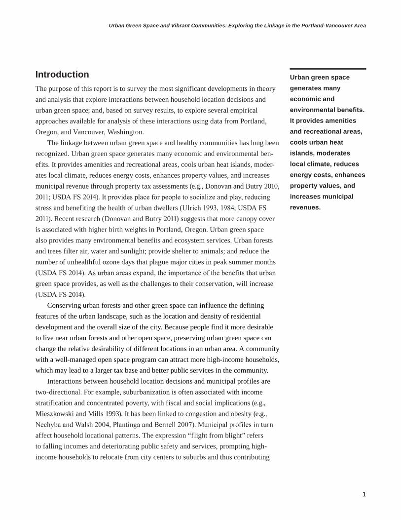
Cover: View of Portland’s 5,100-acre Forest Park adjacent to the city’s downtown and industrial core.

AbstractStone, Edward A.; Wu, JunJie; Alig, Ralph. 2015. Urban green space and vibrant

communities: exploring the linkage in the Portland-Vancouver area. Gen. Tech. Rep. PNW-GTR-905. Portland, OR: U.S. Department of Agriculture, Forest Service, Pacific Northwest Research Station. 43 p.

This report investigates the interactions between household location decisions and community characteristics, including green space. Household location decisions are a primary driver of land-use change, and collective location decisions affect community characteristics. At the same time, community characteristics affect location decisions. Neighborhoods or communities that have well-managed green space programs are more attractive to residents, a two-way interaction that tends to be self-reinforcing. Communities with high amenities and public services attract high-income residents, enhancing the tax base and the provision of amenities and services. This report surveys the literature investigating these interactions and explores several applicable empirical approaches for the Portland, Oregon, and Vancouver, Washington, metropolitan area.

The emergence of spatially explicit data and software facilitates the investiga-tion of relationships between location choice and community characteristics. Using data from Portland, Oregon, and Vancouver, Washington, this report details several possible empirical approaches, including instrumental variables, reduced-form estimation, and treatment effects. The primary challenge for the researcher is the endogeneity of community characteristics.

Keywords: Amenities, community characteristics, population change, residen-tial location choices, urban green space.

1

Urban Green Space and Vibrant Communities: Exploring the Linkage in the Portland-Vancouver Area

1

IntroductionThe purpose of this report is to survey the most significant developments in theory and analysis that explore interactions between household location decisions and urban green space; and, based on survey results, to explore several empirical approaches available for analysis of these interactions using data from Portland, Oregon, and Vancouver, Washington.

The linkage between urban green space and healthy communities has long been recognized. Urban green space generates many economic and environmental ben-efits. It provides amenities and recreational areas, cools urban heat islands, moder-ates local climate, reduces energy costs, enhances property values, and increases municipal revenue through property tax assessments (e.g., Donovan and Butry 2010, 2011; USDA FS 2014). It provides place for people to socialize and play, reducing stress and benefiting the health of urban dwellers (Ulrich 1993, 1984; USDA FS 2011). Recent research (Donovan and Butry 2011) suggests that more canopy cover is associated with higher birth weights in Portland, Oregon. Urban green space also provides many environmental benefits and ecosystem services. Urban forests and trees filter air, water and sunlight; provide shelter to animals; and reduce the number of unhealthful ozone days that plague major cities in peak summer months (USDA FS 2014). As urban areas expand, the importance of the benefits that urban green space provides, as well as the challenges to their conservation, will increase (USDA FS 2014).

Conserving urban forests and other green space can influence the defining features of the urban landscape, such as the location and density of residential development and the overall size of the city. Because people find it more desirable to live near urban forests and other open space, preserving urban green space can change the relative desirability of different locations in an urban area. A community with a well-managed open space program can attract more high-income households, which may lead to a larger tax base and better public services in the community.

Interactions between household location decisions and municipal profiles are two-directional. For example, suburbanization is often associated with income stratification and concentrated poverty, with fiscal and social implications (e.g., Mieszkowski and Mills 1993). It has been linked to congestion and obesity (e.g., Nechyba and Walsh 2004, Plantinga and Bernell 2007). Municipal profiles in turn affect household locational patterns. The expression “flight from blight” refers to falling incomes and deteriorating public safety and services, prompting high-income households to relocate from city centers to suburbs and thus contributing

Urban green space generates many economic and environmental benefits. It provides amenities and recreational areas, cools urban heat islands, moderates local climate, reduces energy costs, enhances property values, and increases municipal revenues.

2

General technical report pnw-Gtr-905

to suburbanization and sprawl. Conversely, high-income communities may enact zoning and tax regimes that affect land-use patterns by attracting new residents or restricting the pattern of development.

In many cases—and in many economic models (e.g., Wu 2006)—the interac-tion between household location choices and municipal profiles is self-reinforcing. “Flight from blight” further diminishes central city incomes and tax revenues, lead-ing to deteriorating public services and safety and thus more flight. High-income suburbs with better public services attract more high-income households. Other urban-development phenomena may also be self-reinforcing, including gentrifica-tion and urban revitalization.

Literature ReviewHousehold preferences and collective location decisions determine land use pat-terns and neighborhood characteristics. Two primary bodies of economic literature attempt to explain historical development patterns through the lens of household locational choice. The urban economics literature, in particular the monocentric city model with early incarnations by Alonso (1964), Mills (1967), and Muth (1969), explains changes in urban land use patterns in terms of rising incomes, falling commuting costs, and newer housing on the periphery. In contrast, the local public finance approach explains development patterns in terms of preferences for alterna-tive bundles of local taxes and public goods and services. This body of literature expands on Tiebout’s (1956) household sorting model.

Although urban economics models capture the primary drivers of the historical development pattern, they do not account for other factors that influence house-hold locational choice within a metropolitan area, including amenities and public finances (Nechyba and Walsh 2004). Local public finance models include these factors and better explain why many households moving to the suburbs prefer to form homogenous groups, but they are typically aspatial. Below we first review the literature on household location decisions and then focus on the interactions between location decisions and municipal profiles.

Household Location DecisionsSuburbanization has been a dominant trend in aggregate household location deci-sions and urban spatial development in the modern era. The classic monocentric city model offers important insights into this phenomenon. In this model (Alonso 1964, Mills 1967, Muth 1969), all employment lies within the central business district (CBD), households are differentiated by income, and the key difference between alternative household locations is distance to the CBD. Because housing

3


close to the employment center is relatively expensive, households face a tradeoff between commuting time and housing price. Those who choose to live farther away incur higher commuting costs but face lower housing prices and can thus afford to consume more housing. The primary driver behind suburbanization and modern urban spatial development has been falling commuting cost owing to the prolifera-tion of the automobile and the development of highway systems. Simple CBD models account for this driver and correctly predict expanding urban footprints in the face of decreasing transportation costs. However, simple CBD models do not account for a number of other relevant factors—including alternative transportation modes, locational amenities, and age of the housing stock—nor do they predict multicentric metropolitan areas and various historical development patterns that we observe. A number of researchers have relaxed assumptions and generalized CBD models to address these concerns.

LeRoy and Sonstelie (1983) incorporated two alternative transport modes—one fast and one slow—and demonstrated that when more affluent households are bet-ter able to afford the faster mode, they will tend to suburbanize more rapidly than others. They argued that this was the case early on with the automobile. However, as the cost of the faster mode falls (the vast majority of American households can now afford to commute by car), more affluent households lose this comparative advantage for suburbanizing. In fact, because wages—and thus opportunity cost of time—are higher for high-earners, LeRoy and Sonstelie (1983) predicted gen-trification by more affluent households as commuting costs fall and less affluent households suburbanize. According to this model, when high- and low-income households use the same transport mode, high-income households will tend to locate in the city center.

Brueckner et al. (1999) added natural and historical amenities to explain alternative income distributions across different cities. They observed the stark difference between most American cities, where high-income households tend to live in the suburbs, and many European cities, where the wealthy occupy the central city.1 Their model explains these differences in terms of differing levels of natural and historical amenities across cities. As with classic CBD models, the rich are pulled to the suburbs by their preference for more housing, which is available more

1 The simple CBD model is consistent both with higher income households locating in the center (the ratio of commuting cost per mile to housing consumption increases with income) and with higher income households locating in the suburbs (opposite). However, it seems implausible that the behavior of this ratio across countries differs enough to fully explain differences in spatial income distribution. See Brueckner et al. (1999) for a more complete discussion.

There is a stark difference between most American cities, where high-income households tend to live in the suburbs, and many European cities, where the wealthy occupy the central city.

4


cheaply on the periphery; simultaneously, they are pulled into the center by the high time-cost of commuting. However, this model also allows for heterogeneous levels of natural and historical amenities between the center and the suburbs. When the central city has high levels of amenities, like Paris, these constitute an additional attraction for the wealthy. On balance, the time-cost effect and the amenity effect outweigh the housing price effect, and the wealthy locate in the center. When the central city has low or even negative amenity value, such as in Detroit, the housing price effect dominates, and the wealthy locate in the suburbs. A key assumption of this model is that preferences for amenities rise with income.

Wu (2006) incorporated amenities in a different fashion. Distinguishing between exogenous amenities (natural and historical features) and endogenous amenities (e.g., local public services), this study incorporated exogenous amenities in a modified CBD model. Alternative locations within the city differ in terms of the distance to the employment center and the level of local amenities. In contrast to the model presented by Brueckner et al. (1999), spatially heterogeneous amenities in this model attract households to various suburbs. With this spatial heterogeneity in amenities, households may be willing to pay more for a nice location than for a short commute; thus, housing prices may not fall uniformly as we move away from the center. At a given distance from the center, higher income households will choose locations with better amenities. This model is consistent with noncontiguous development patterns and non-distance-based patterns of income segregation. Wu (2006) included a model incorporating endogenous amenities as well, discussed below with local public finance models.

Brueckner and Rosenthal (2009) posited that the age of housing stock is an important determinant of the location of high- and low-income households. The resulting model is consistent with both suburbanization and gentrification. In addition to short commutes and low housing prices, high-income households prefer newer housing. Commuting concerns pull households inward; housing price concerns pull them outward. The location of new or newly remodeled housing determines the direction of the housing-age effect. As a city grows, new housing is always available on the periphery. Some new housing is also available in the inte-rior—more so during periods of rapid redevelopment. If new housing is abundant in the interior city, it exerts an additional pull, causing some high-income households to locate in the center. Holding housing age constant, this model predicts a negative relationship between income and distance—the rich prefer to live in the center. Contrast this with the traditional CBD model, in which suburbanization by the rich implies a positive relationship between income and distance.

5


Central business district models, including those discussed above, assume monocentricity—that is, all firms (and thus all employment) locate in the CBD. Whereas household location is determined endogenously within the model, firm location is given exogenously. Ogawa and Fujita (1980) and Fujita and Ogawa (1982) relaxed this assumption and explored the conditions under which a non-monocentric city is the equilibrium urban spatial configuration. In addition to commuting cost, these models include a transaction cost parameter that measures the benefits of spatial clustering for firms. When transaction costs are high relative to marginal commuting costs, the incentive for firms to cluster outweighs the incen-tive for households to locate close to work. A monocentric city is the equilibrium spatial arrangement. Higher relative marginal commuting costs give rise to multiple dispersed employment centers, as households have increasingly strong incentives to minimize commuting distance. In the extreme case in which firms do not benefit from spatial proximity, the equilibrium spatial arrangement is a fully mixed city with firms and residences dispersed throughout.

Interactions Between Location Decisions and Municipal ProfilesLocal public finance models offer an alternative lens through which to examine household locational choice. Even broadened to include amenities, housing age, and transit considerations, CBD models do not fully capture the role of community characteristics. Dating back to Tiebout (1956), local public finance models endoge-nize the provision of public services. In other words, these models account for the interaction between household locational choice and the levels of local taxes and public services. Households choose a location based in part upon their preferences for various bundles of local taxes and public services at the community scale. They “vote with their feet.” Simultaneously, households influence the level of taxes and services in a community through the representative process and through their tax contributions and impacts on neighbors. A brief discussion of the link between household locational choice and community characteristics follows.

A household chooses a home based on income/wealth, owner preferences, home characteristics, and community characteristics. Based on their finances, families choose a preferred option from available house-community combinations. The role of community characteristics in this process is clear: families like nice, safe neigh-borhoods and good school districts. The link between household location decisions and community characteristics is more involved. Relevant community charac-teristics include tax rates and the levels of amenities and public services. Some community characteristics, primarily amenities, are truly unaffected by household location decision. Consider natural features, such as hills, lakes, or rivers, or a

6


well-established man-made attraction, like a historical site or a bustling commercial district. These types of sites exist prior to any location decisions and will persist regardless of those decisions. Other community characteristics are endogenous; they are affected by household location decisions.

Collective location decisions—and the preferences and characteristics of the resulting population—affect these endogenous community characteristics in three ways: voting, local public finance externalities, and peer externalities. First, community residents vote for their preferred bundle of taxes and services. As the voter base changes owing to household relocations, the results of these votes may change. Voting determines the local tax rate directly, but relocation decisions can alter the size of the tax base, affecting local public service provision indirectly. If high-income households move out of central cities and into suburbs in clas-sic “flight-from-blight,” we would expect an erosion of the city tax base and a strengthening of the suburban tax base, leading to deteriorating public services in the center and enhanced services in the suburbs. This is the local public finance externality. Collective location decisions that shift income distributions affect the ability of jurisdictions to provide services. Finally, peer externalities also affect the level or quality of service independently of finances. Consider public education, for example. Funding affects school quality, and wealthier school districts tend to be better-funded—the local public finance externality. Highly involved parents may also affect school quality. So, two comparably funded districts with different levels of parental engagement might expect different results. Peer externalities are present when the level of the public service provided depends on the characteristics of the population being served as well as the level of funding. Interestingly, peer externali-ties may preclude the possibility of leveling the playing field by increasing funding to lagging communities. Desire to take advantage of perceived peer externalities may influence location decision and has been put forth as an explanation for the formation of homogenous suburbs (Nechyba and Walsh 2004).

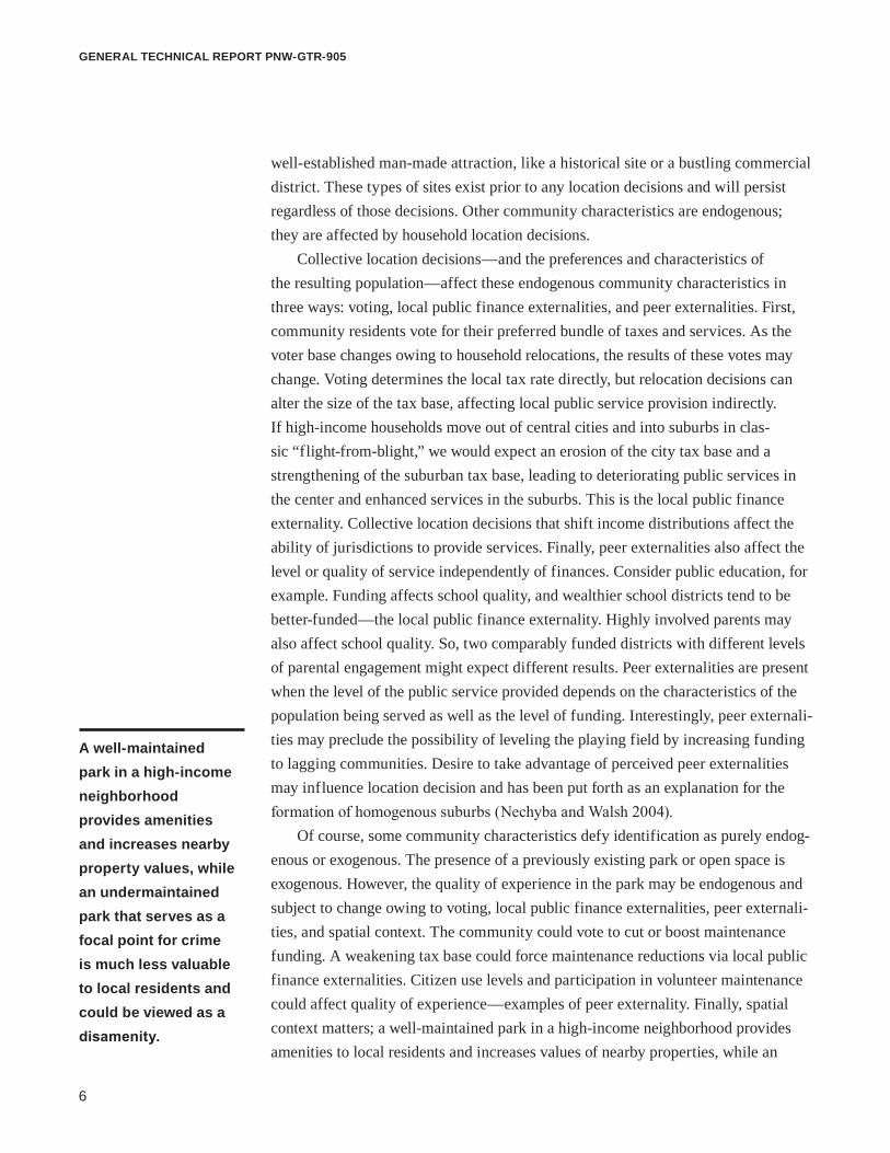
Of course, some community characteristics defy identification as purely endog-enous or exogenous. The presence of a previously existing park or open space is exogenous. However, the quality of experience in the park may be endogenous and subject to change owing to voting, local public finance externalities, peer externali-ties, and spatial context. The community could vote to cut or boost maintenance funding. A weakening tax base could force maintenance reductions via local public finance externalities. Citizen use levels and participation in volunteer maintenance could affect quality of experience—examples of peer externality. Finally, spatial context matters; a well-maintained park in a high-income neighborhood provides amenities to local residents and increases values of nearby properties, while an

A well-maintained park in a high-income neighborhood provides amenities and increases nearby property values, while an undermaintained park that serves as a focal point for crime is much less valuable to local residents and could be viewed as a disamenity.

7


undermaintained park that serves as a focal point for criminal behavior is much less valuable to local residents and could potentially be viewed as a disamenity (Ander-son and West 2006, Troy and Grove 2008).

By incorporating interaction between community characteristics and household location decisions, local public finance models go beyond their CBD counterparts. Following Tiebout’s seminal 1956 paper, other researchers expanded on Tiebout’s general equilibrium model. Ellickson (1971) derived the single-crossing property, a necessary condition for equilibrium characterized by income stratification. Epple et al. (1984) incorporated housing markets. Epple and Sieg (1999) developed a general method for estimating equilibrium models of local jurisdictions. Although these studies generate strong predictions of characteristics of communities in equilib-rium—including income stratification across communities or, more generally, income stratification across communities by preference—they ignored location.

Wu (2006) incorporated distance and exogenous amenities in a hybrid of CBD and local public finance models. The first model from this paper, mentioned above, simply adds exogenous amenities to a CBD model. A second model, however, includes both exogenously determined amenities and endogenously determined taxes and public services. This model predicts income stratification by amenity level for a given distance from the city center.

In addition to urban economics and local public finance, papers from several economic sub-genres informed our investigation of the link between land use and municipal profiles. Hedonic home pricing offers insight into the preferences driv-ing household location choice, which in turn drives land-use change. Oates (1969) introduced hedonic modeling to test Tiebout’s hypothesis, and a wide range of empirical studies use hedonics to estimate the value of community characteristics (both positive and negative) as capitalized in home sale prices (e.g., Anderson and West 2006, Bowes and Ihlanfeldt 2001, Cohen and Coughlin 2008, Troy and Grove 2008).

One clear message emerges from this literature: when one is estimating the effect of amenities (or disamenities) on home prices, spatial context matters. For example, Cohen and Coughlin (2008) found that the effect of proximity to an airport varies with distance. If you are too close, airport noise drives down home prices; if sufficiently far away to mitigate noise, proximity to the airport drives up home prices. Troy and Grove (2008) found that although some parks are amenities and exert a positive effect on home prices, parks in high crime areas may be seen as a disamenity or liability, and thus proximity to them may be correlated with lower home prices. In this case, negative spatial context renders the willingness to pay for proximity to a park negative. Other studies have found that the amenity value

8


of open space varies widely with distance from the city center (Geoghegan et al. 1997), whether the site is permanently designated as open space (Irwin and Bock-stael 2001), the type and proximity of open space (e.g., Anderson and West 2006, Smith et al 2002), and income and age structure of the neighborhood (Anderson and West 2006), to name a few. Recent research indicates that the presence of an additional bird species increases home prices by approximately $32,000 (Farmer et al. 2013). Similarly, Donovan and Butry (2010) found that the presence of street trees increases home sales price and reduces time on market. Investigating how households value particular community characteristics—and how those values vary depending on context—enhances our understanding of household location decisions.

Related research documents the positive effects of urban trees on home rental prices (Donovan and Butry 2011), crime (Donovan and Prestemon 2012), and health (Donovan et al. 2011). The Green Cities Research Alliance, a collaborative effort between the Forest Service and various research entities in the Pacific Northwest, is a good source for emerging research on the interaction between urban areas and the environment, including the studies listed above.

Beyond hedonics, a number of papers have focused on urban sprawl. The term sprawl has negative connotations and is often cited as an example of a land-use pat-tern with negative social implications. Nechyba and Walsh (2004) provided a com-prehensive review of the literature on sprawl. They argued that, despite its negative reputation, sprawl occurs because individual households are happier with the larger homes and lots that it offers. However, they did identify four costs: road congestion, vehicle pollution, loss of open space, and unequal service and public good provision across metropolitan areas resulting from self-segregation and associated pockets of affluence and poverty. Lopez (2004) and Plantinga and Bernell (2007) investigated the link between obesity and urban sprawl. These papers and most of the related literature focused on concrete impacts of sprawl: weight, emissions, and income distribution. Brueckner and Largey (2008) notably departed from this trend and focused on sprawl and the reduction of social interaction. They investigated the premise that low-density living reduces social interaction to the detriment of society as a whole.

A well-developed economics literature exists on household locational choice. Although less well studied, a number of papers focus on the role of race. For example, Bayer and McMillan (2005) developed a sorting model that includes race and conducted simulations to illustrate the effect of race. They found that racial sorting contributes to the racial disparity in neighborhood amenity consumption, though that sorting could be the result of discrimination or simply a preference to

9


live among like households. Ihlanfeldt and Sjoquist (2000) provided a review of related studies. This literature sheds light on our race results, described in detail below. The economic processes and implications involved will be the focus of future research.

In the sections that follow, we apply lessons from the above literature to inves-tigate a case study of household locational choice. First, we explore the data sources and processing methods. Then, we discuss appropriate econometric models and estimation challenges.

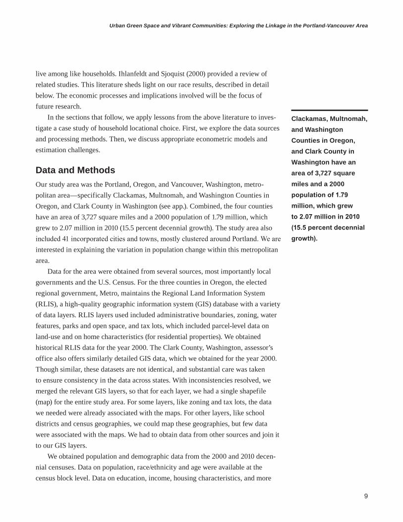
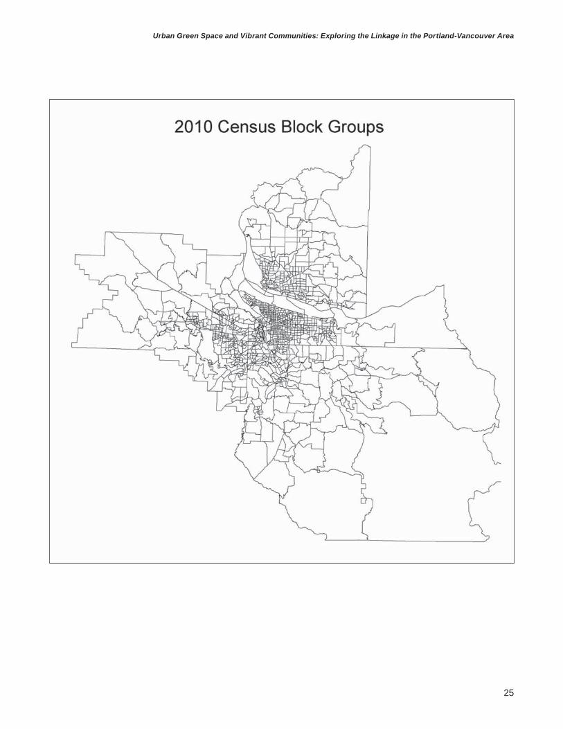
Data and MethodsOur study area was the Portland, Oregon, and Vancouver, Washington, metro-politan area—specifically Clackamas, Multnomah, and Washington Counties in Oregon, and Clark County in Washington (see app.). Combined, the four counties have an area of 3,727 square miles and a 2000 population of 1.79 million, which grew to 2.07 million in 2010 (15.5 percent decennial growth). The study area also included 41 incorporated cities and towns, mostly clustered around Portland. We are interested in explaining the variation in population change within this metropolitan area.

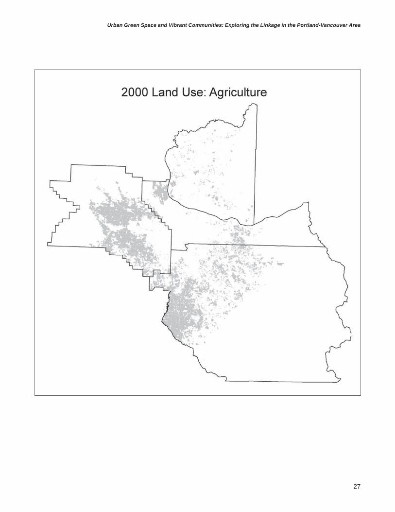
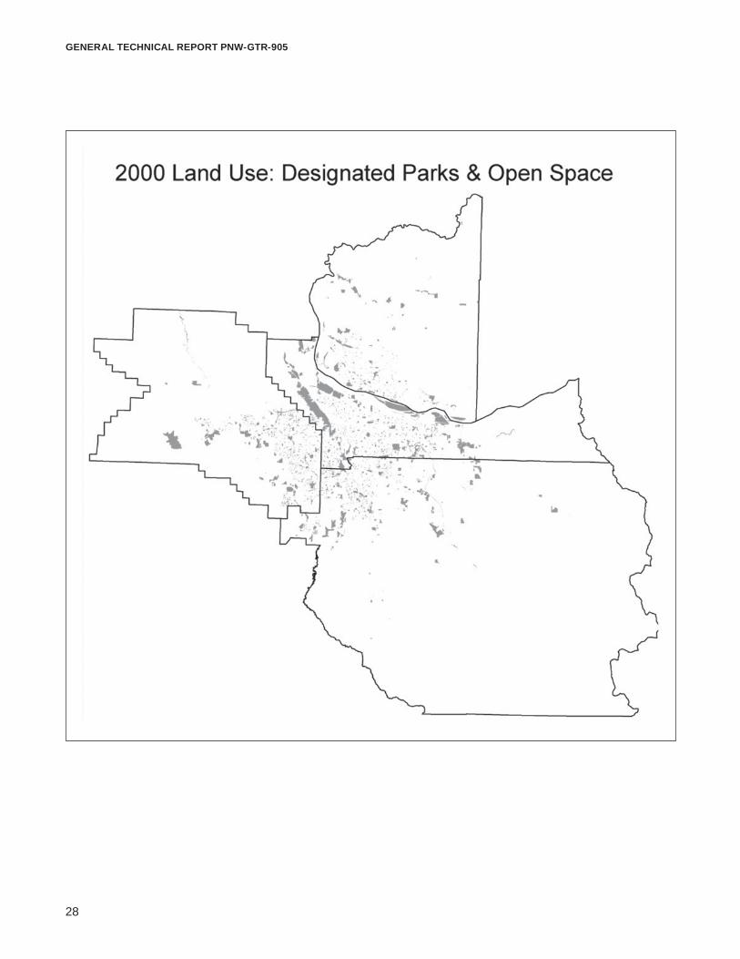
Data for the area were obtained from several sources, most importantly local governments and the U.S. Census. For the three counties in Oregon, the elected regional government, Metro, maintains the Regional Land Information System (RLIS), a high-quality geographic information system (GIS) database with a variety of data layers. RLIS layers used included administrative boundaries, zoning, water features, parks and open space, and tax lots, which included parcel-level data on land-use and on home characteristics (for residential properties). We obtained historical RLIS data for the year 2000. The Clark County, Washington, assessor’s office also offers similarly detailed GIS data, which we obtained for the year 2000. Though similar, these datasets are not identical, and substantial care was taken to ensure consistency in the data across states. With inconsistencies resolved, we merged the relevant GIS layers, so that for each layer, we had a single shapefile (map) for the entire study area. For some layers, like zoning and tax lots, the data we needed were already associated with the maps. For other layers, like school districts and census geographies, we could map these geographies, but few data were associated with the maps. We had to obtain data from other sources and join it to our GIS layers.

We obtained population and demographic data from the 2000 and 2010 decen-nial censuses. Data on population, race/ethnicity and age were available at the census block level. Data on education, income, housing characteristics, and more

Clackamas, Multnomah, and Washington Counties in Oregon, and Clark County in Washington have an area of 3,727 square miles and a 2000 population of 1.79 million, which grew to 2.07 million in 2010 (15.5 percent decennial growth).

10


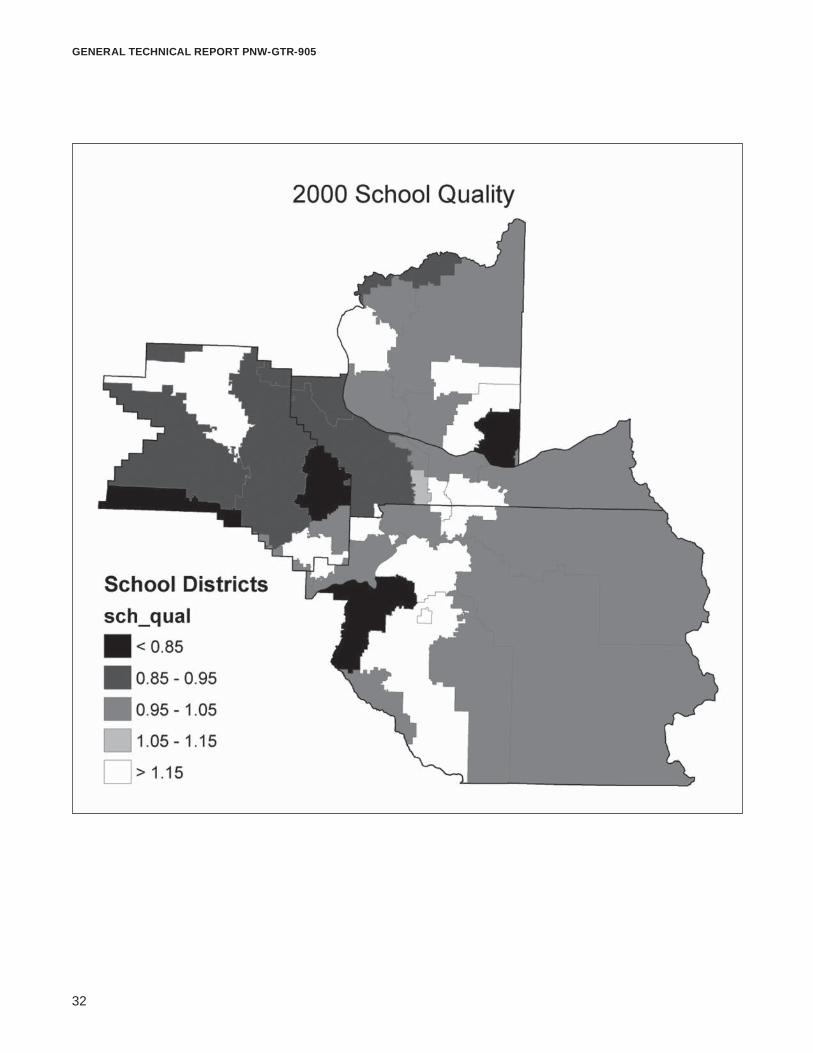
were available at the block group level. To give an idea of scale, in 2000 our study area contained 34,178 census blocks and 1,160 block groups. We also obtained redistricting data from the 2010 census, which included population and race/ethnic-ity data. Additional data sources included county governments for property tax levy rates, state departments of education for school quality data, and the USDA Forest Service for national forest maps.

With underlying data in place, the next step was choosing units of observation. Existing geographies tend to be problematic. Using counties would provide only four observations and ignore variation in population change and local municipal profiles within the counties. Using cities drops unincorporated areas and again ignores variation, particularly in the largest city, Portland. U.S. Census geographies, including census blocks and census block groups, are much smaller than coun-ties and cities and so can capture variation within cities and counties. However, a considerable proportion of census geographies shift boundaries over time, leading to consistency problems when measuring population change. Furthermore, the size of census geographies varies widely, as census blocks and block groups are drawn to have roughly equal populations. Thus rural census blocks with low population density are much larger than densely populated urban census blocks. Finally, census geography boundaries are not random, but tend to follow evident development pat-terns and form homogenous units. While these make sense as cohesive units within a city or county, nonrandom boundaries can lead to endogeneity issues and biased estimates (Banzhaf and Walsh 2008).

We avoided problems associated with existing geographies by adopting an approach suggested by Banzhaf and Walsh (2008). Specifically, a grid of 2-mile squares was laid over a map of the metro area, then a circle 2 miles in diameter was drawn centered in each square. We dropped circles that were not completely within our four counties, leaving a sample of 844 circular observations. We did not consider these to represent communities in any social or political sense. Rather, this method constituted an effective sampling methodology, which allowed us to take advantage of high-resolution spatial data.

Of course, a grid of circles 2 miles in diameter is not the only option. Alterna-tive diameters, shifting the grid incrementally, and random locations as opposed to a grid are possible. Using hexagons or squares rather than circles would provide full coverage of the study area. Comparing alternative units is a good strategy for testing the sensitivity of parameter estimates. Parameters which are highly sensitive to the spatial sampling unit should be viewed with skepticism.

With units selected, we used GIS software and data to quantify variables measuring characteristics for each observation. This procedure differs depending

11


on the data in question. Some GIS layers covered the entire study area, like census geographies, tax lots, zoning, and school districts. These layers each contained one or more potential explanatory variables. For each layer, a GIS script aggregated the variables of interest from the underlying geometry to our circular observations. Specifically, the script computed an area-weighted sum for each variable. The number of elements in this weighted sum varied with the data layer in question. For example, school districts tend to be large, so most circles fell into one or only a few school districts. On the other hand, tax lots are much smaller. In dense residential areas within the city, some circles may contain thousands of tax lots. The number of elements in the weighted sum also varies in space for the same data layer. For instance, census block groups are small in densely populated, central areas and big in less populated areas far from the city center. So, some more remote circles fall entirely within one block group while in the center a single circle intersected dozens of block groups.

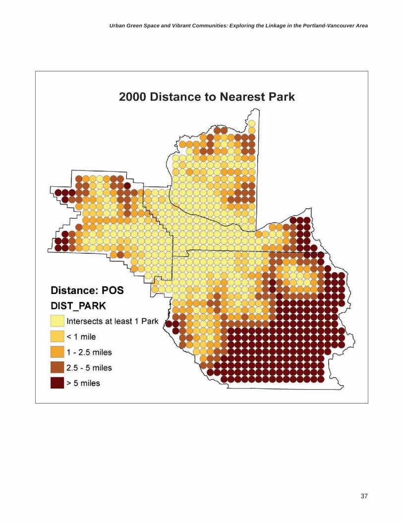
For GIS layers that contain only points, such as bus stops, the appropriate measure might be the number of bus stops in a circular observation. Access to parks is another example. We could measure access in a variety of ways: park acreage within the circle, distance to the nearest park, and number or acreage of parks within some distance, to name a few. Wu and Plantinga (2003) emphasized distance as a superior measure of open space access. Distances from each observation to the city center and the nearest parks and open spaces were also computed.

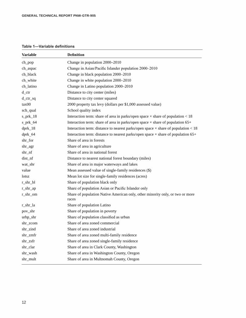
The final step in preparing our data was building interaction terms. The hedonics literature reveals variations in amenity values depending on many factors including income, proximity, age, urban density, and crime, to name a few. Interac-tion terms allow the researcher to model differential effects. For example, a park located in a low-income, high-crime neighborhood may not be valued as highly as a park in a high-income, low-crime neighborhood. A model including interaction terms between crime or income and park proximity might pick up this differential effect, whereas an alternative specification would not. Anderson and West (2006) provided a good discussion and a hedonic model with several classes of open space and multiple interaction terms. The interaction terms included in table 1 represent a small subset of the possible interaction terms.

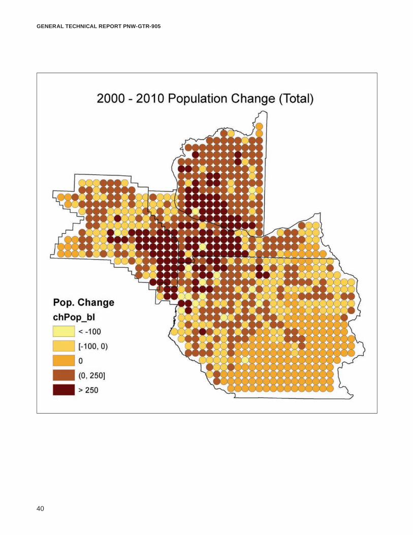
Table 1 defines our variables. Note that only our dependent variables and those explanatory variables included in our model appear, although we did consider and test a number of alternative specifications and alternative variables. Population changes for the entire population and by race are located above the line in table 1. Population change is our primary dependent-variable candidate, as it is a proxy for household locational choice, particularly with uniform circular observations.

12


Table 1—Variable definitions

Variable Definition

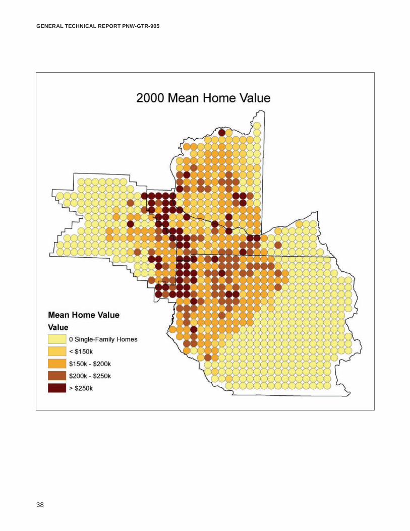
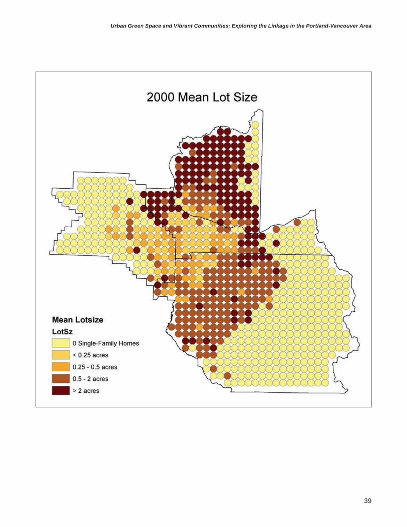
ch_pop Change in population 2000–2010ch_aspac Change in Asian/Pacific Islander population 2000–2010ch_black Change in black population 2000–2010ch_white Change in white population 2000–2010ch_latino Change in Latino population 2000–2010d_ctr Distance to city center (miles)d_ctr_sq Distance to city center squaredtax00 2000 property tax levy (dollars per $1,000 assessed value)sch_qual School quality indexs_prk_18 Interaction term: share of area in parks/open space × share of population < 18s_prk_64 Interaction term: share of area in parks/open space × share of population 65+dprk_18 Interaction term: distance to nearest parks/open space × share of population < 18dprk_64 Interaction term: distance to nearest parks/open space × share of population 65+shr_for Share of area in forestsshr_agr Share of area in agricultureshr_nf Share of area in national forestdist_nf Distance to nearest national forest boundary (miles)wat_shr Share of area in major waterways and lakesvalue Mean assessed value of single-family residences ($)lotsz Mean lot size for single-family residences (acres)r_shr_bl Share of population black onlyr_shr_ap Share of population Asian or Pacific Islander onlyr_shr_om Share of population Native American only, other minority only, or two or more

racesr_shr_la Share of population Latinopov_shr Share of population in povertyurbp_shr Share of population classified as urbanshr_zcom Share of area zoned commercialshr_zind Share of area zoned industrialshr_zmfr Share of area zoned multi-family residenceshr_zsfr Share of area zoned single-family residenceshr_clar Share of area in Clark County, Washingtonshr_wash Share of area in Washington County, Oregonshr_mult Share of area in Multnomah County, Oregon

13


Because all observations are identically sized and shaped, modeling population change is equivalent to modeling change in population density. We included popula-tion change by race as well, because preliminary ordinary least squares analysis (results omitted here due to sheer volume) indicated that race is a persistently significant factor affecting household location choice. Our raw school data was obtained from the state departments of education. Because the test scores vary by state, we constructed an index. In each school district, school quality was defined as the district score over the state average, so the values are bounded below by zero and centered around one. This is just one of several alternative indices we explored. A number of variables measure access to parks, open space, and natural amenities.

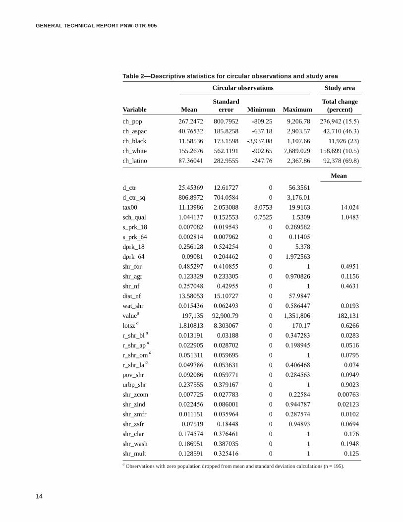
Table 2 provides descriptive statistics for both our circular observations and the study area. For our circles, note that the reported means are unweighted. Most means were taken across all 844 observations, but several omitted circles with zero population to avoid misleading results. Also, several means for the study area differed greatly from the means for our observations. This is not a problem. Rather it is an artifact of averaging spatially aggregated data. Consider lot size. For the study area mean, every residential property gets equal weight in the average. For the mean across our circular observations, we first calculated an average lot size for each circle, then averaged those values. This process in essence gave large lots more weight, as it took fewer of them to fill a circle.

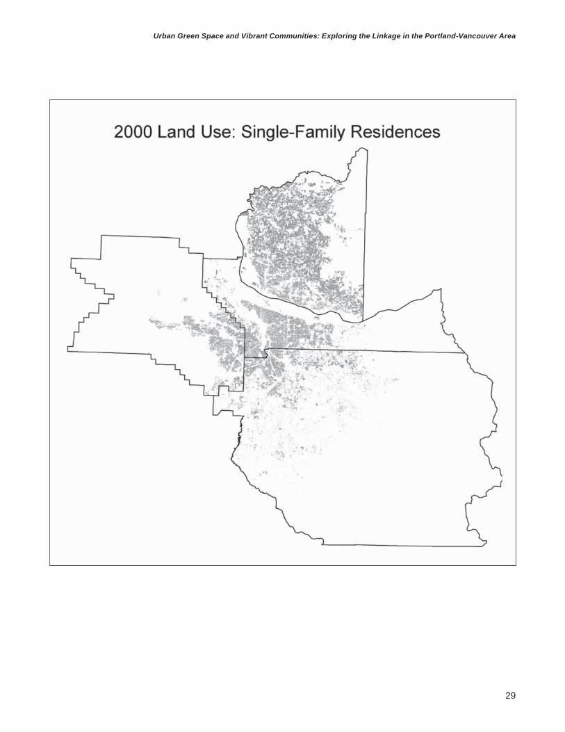
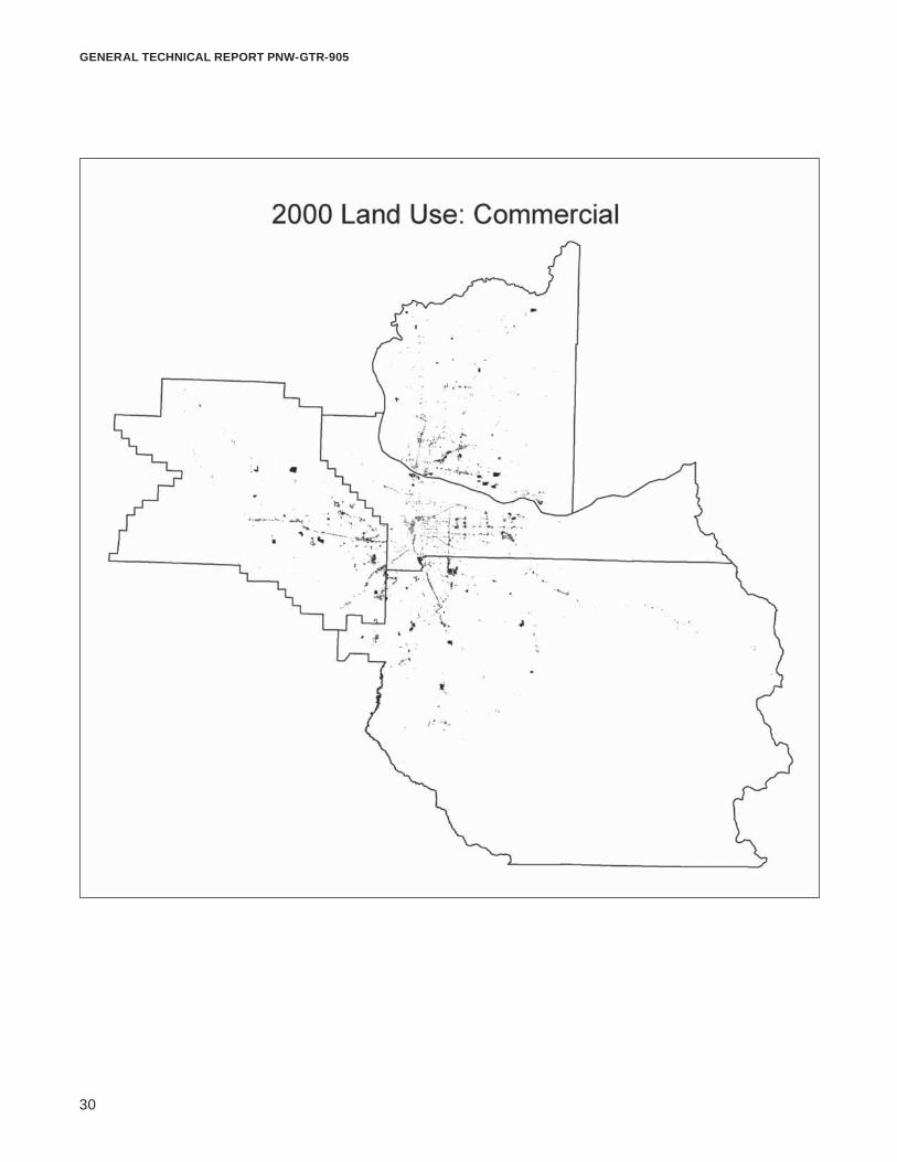
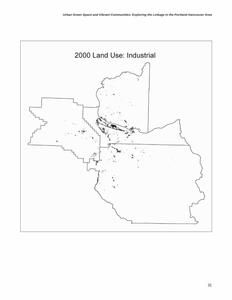
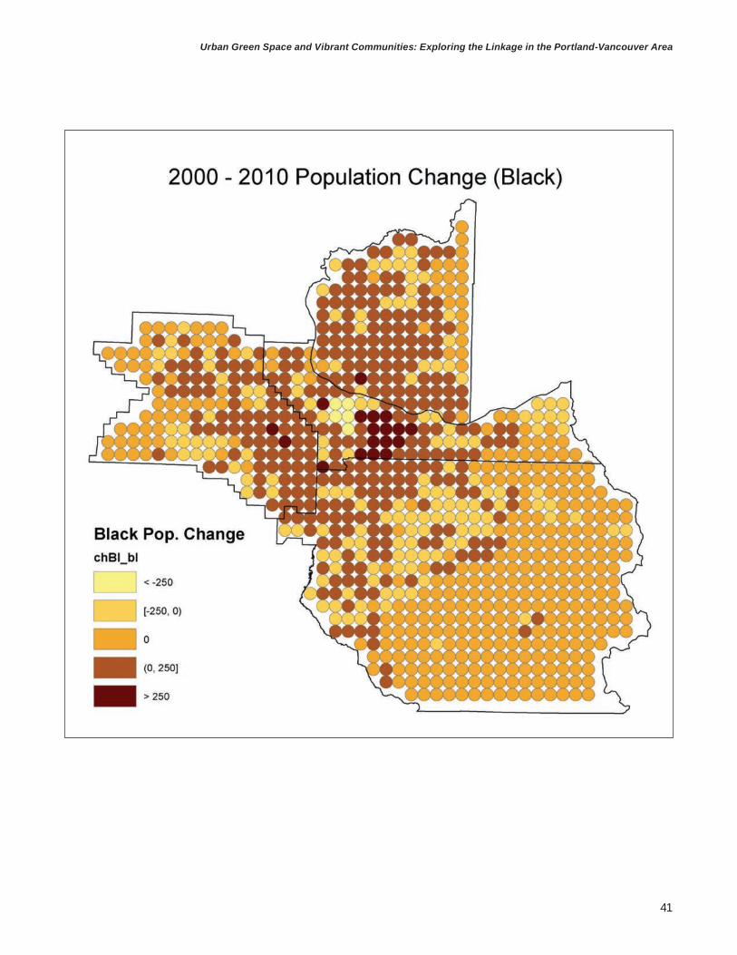
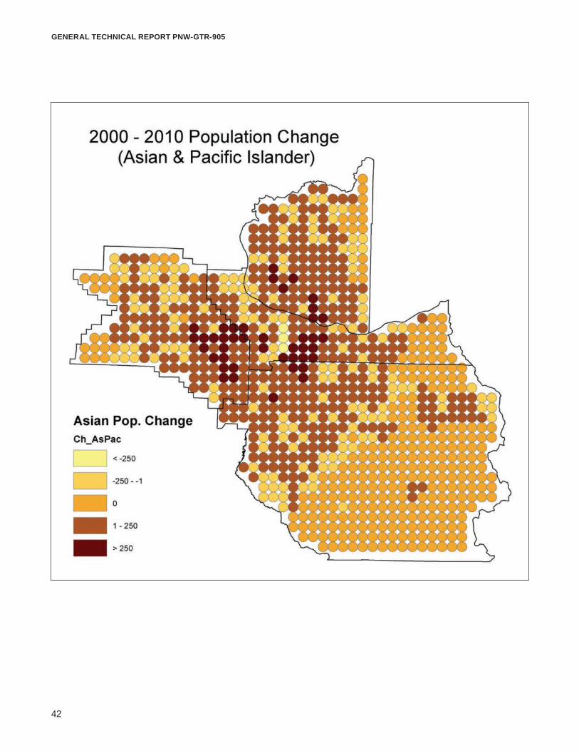
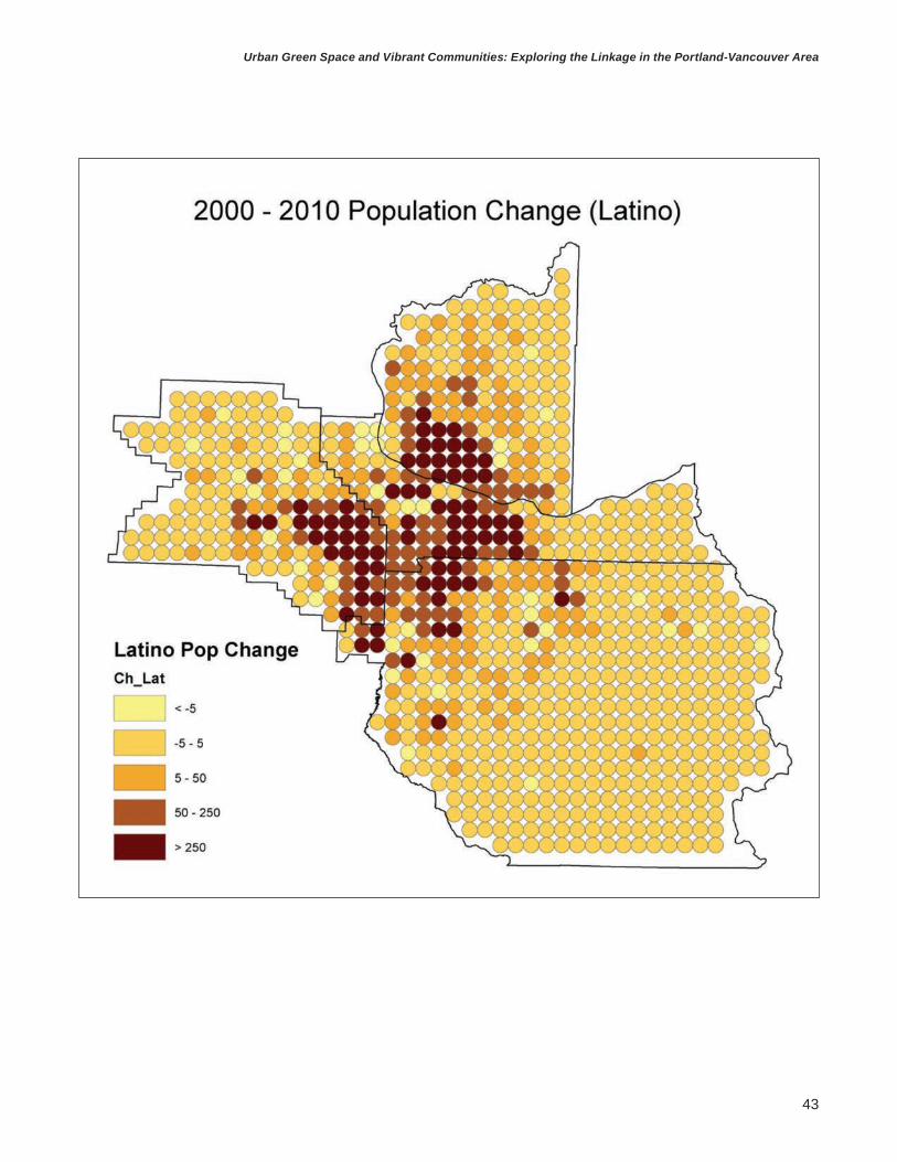
In many cases, these data are easiest to grasp visually in maps. A wide range of maps of both the underlying data and our 2-mile constructed observations are available in the appendix.

Estimation StrategiesThe previous section explored the process of data collection, construction of units of observation, and quantification of variables. Although specific to the Portland, Oregon, and Vancouver, Washington, metropolitan area, this process is applicable to other regions and research questions. With data in place, the challenge is to specify an appropriate model to identify the causal relationships between popula-tion change and various aspects of local municipal profile. Several estimation strategies are available to the researcher investigating household locational choice and municipal profiles.

Structural modeling— The appropriate estimation strategy depends upon the precise research question. In all cases, an appropriate estimation strategy must account for the fact that some variables measuring local municipal profiles are exogenous, while others are endog-enous. Examples of exogenous variables include natural features, parks and open

14


Table 2—Descriptive statistics for circular observations and study area

Circular observations Study area

Variable MeanStandard

error Minimum MaximumTotal change

(percent)

ch_pop 267.2472 800.7952 -809.25 9,206.78 276,942 (15.5)ch_aspac 40.76532 185.8258 -637.18 2,903.57 42,710 (46.3)ch_black 11.58536 173.1598 -3,937.08 1,107.66 11,926 (23)ch_white 155.2676 562.1191 -902.65 7,689.029 158,699 (10.5)ch_latino 87.36041 282.9555 -247.76 2,367.86 92,378 (69.8)

Mean

d_ctr 25.45369 12.61727 0 56.3561d_ctr_sq 806.8972 704.0584 0 3,176.01tax00 11.13986 2.053088 8.0753 19.9163 14.024sch_qual 1.044137 0.152553 0.7525 1.5309 1.0483s_prk_18 0.007082 0.019543 0 0.269582s_prk_64 0.002814 0.007962 0 0.11405dprk_18 0.256128 0.524254 0 5.378dprk_64 0.09081 0.204462 0 1.972563shr_for 0.485297 0.410855 0 1 0.4951shr_agr 0.123329 0.233305 0 0.970826 0.1156shr_nf 0.257048 0.42955 0 1 0.4631dist_nf 13.58053 15.10727 0 57.9847wat_shr 0.015436 0.062493 0 0.586447 0.0193valuea 197,135 92,900.79 0 1,351,806 182,131lotsz a 1.810813 8.303067 0 170.17 0.6266r_shr_bl a 0.013191 0.03188 0 0.347283 0.0283r_shr_ap a 0.022905 0.028702 0 0.198945 0.0516r_shr_om a 0.051311 0.059695 0 1 0.0795r_shr_la a 0.049786 0.053631 0 0.406468 0.074pov_shr 0.092086 0.059771 0 0.284563 0.0949urbp_shr 0.237555 0.379167 0 1 0.9023shr_zcom 0.007725 0.027783 0 0.22584 0.00763shr_zind 0.022456 0.086001 0 0.944787 0.02123shr_zmfr 0.011151 0.035964 0 0.287574 0.0102shr_zsfr 0.07519 0.18448 0 0.94893 0.0694shr_clar 0.174574 0.376461 0 1 0.176shr_wash 0.186951 0.387035 0 1 0.1948shr_mult 0.128591 0.325416 0 1 0.125a Observations with zero population dropped from mean and standard deviation calculations (n = 195).

15


space, and historical development patterns. Examples of endogenous variables in-clude median household income, school quality, and property tax rate. The quantity of urban trees in a given area and the extent of canopy cover are additional exam-ples of endogenous variables, as trees are cut and planted during the residential de-velopment (or redevelopment) process. In the absence of endogeneity, the researcher could simply regress population change on variables quantifying municipal profile. Owing to endogeneity, this simple approach would yield biased estimates. Because some of the explanatory variables are affected by the dependent variable and thus correlated with the error term, the model becomes a system of simultaneous equa-tions. In structural form, model looks like:

Y = Xnβn+Xsβ+εy, (1)

i i i i is y n n z xX Y X Zγ γ γ ε= + + + , i=1, 2, …, n (2)

where Y is the population change vector, Xn is exogenous municipal profile vari-ables such as elevation and total water area, 1 2( , ,..., )n

s s s sX X X X= is the endog-enous municipal profile variables such as school quality and acreage of green space,

iZ is a vector of variables that affect endogenous profile variable i, but do not affect household location choices directly, the β’s and γ’s are the respective coef-ficients, and the ε’s are the error terms. The structural model can be estimated in different ways, depending on the availability of appropriate instrumental variables and data.

If variables iZ can be identified for each endogenous profile variable, and data on iZ are available, then 1 2( , ,..., )nZ Z Z can serve as a set of instrumental variables because they are correlated with the endogenous explanatory variable and uncorrelated with the error term (i.e., causally unrelated to the dependent variable). In this case, the structural model can be estimated using second or third stage least squares or partial or full information maximum likelihood estimation methods. For example, using two-stage least squares, first regress each endogenous variable in Xs on all exogenous variables in the model 1 2( , ,..., )nZ Z Z and Xn) and obtain fitted values, 𝑋𝑋𝑋𝑋𝑠𝑠𝑠𝑠� . Then replace endogenous variables with fitted values in (1) in the second stage regression.

(3)

Estimates derived from instrumental variables and two-stage least squares are only as reliable as the instruments. If the chosen instruments are correlated with the error term, the bias problems encountered in the structural form remain unre-solved. If the chosen instruments are poor (weakly correlated with the endogenous variables they are replacing), the result is poor fitted values with little variation

𝑌𝑌𝑌𝑌 = 𝑋𝑋𝑋𝑋𝑛𝑛𝑛𝑛𝛽𝛽𝛽𝛽𝑛𝑛𝑛𝑛 + 𝑋𝑋𝑋𝑋𝑠𝑠𝑠𝑠�𝛽𝛽𝛽𝛽𝑠𝑠𝑠𝑠 + 𝜀𝜀𝜀𝜀𝑦𝑦𝑦𝑦

16


generated in the first stage. For this case study, appropriate instruments would need to be correlated with endogenous amenities, uncorrelated with the error term, and not included in the set of explanatory exogenous amenities. It can be challenging to identify such variables.

Reduced-form estimation— When appropriate instruments are not available, researchers may resort to estimating the reduced form of the structural model to uncover useful infor-mation about the effect of amenities on location choices. Solving for Y and

1 2( , ,..., )ns s s sX X X X= , one can derive each of these endogenous variables as a

function of 1 2( , ,..., )nZ Z Z and Xn. These reduced-form equations can then be estimated using an appropriate method. The related literature strongly suggests that exogenous natural amenities influence development patterns, and these devel-opment patterns in turn affect the level of endogenous social amenities (e.g., Wu 2006). Thus exogenous variables can be used to explain endogenous variables. The reduced form approach has a major drawback: estimation does not identify the structural coefficients found in equation 1. So, while estimating the reduced form in this case sheds light on how natural amenities affect the level of social amenities, it does not reveal the effects of various elements of municipal profile on population change.

The model specification in equation 1 potentially includes multiple endogenous covariates, e.g., tax rate, school quality, and park access. This case study has a broad research question. How do elements of municipal profile affect population change? By narrowing the research question to focus on a single endogenous covariate, asking instead how property tax rate affects population change, a number of other estimation strategies from the treatment effects literature become available. Ordinary least squares (OLS) estimation of treatment effects is typically biased because treatment effectiveness depends on factors that determine whether an observation gets treated. In a medical context, the effectiveness of medical interven-tion depends on the characteristics of the patient. At the same time, the character-istics of the patient determine whether the patient receives the treatment. Although a full discussion of treatment effects is beyond the scope of this paper, a number of measures developed for nonexperimental settings in the medical field are increas-ingly being adopted by economists.

Treatment effects— Two relevant estimation strategies from this literature are propensity score match-ing and difference-in-difference estimators, both described below in the context of

17


property taxes. Propensity score matching could be used to evaluate the effect of differential tax rates on population growth. Propensity score matching estimates the treatment effect by systematically comparing pairs of observations from the treat-ment and non-treatment groups that are otherwise alike. This method first estimates a model predicting likelihood of treatment and pairs observations for comparison based on the resulting fitted values. For property taxes, this would involve identi-fying low- and high-tax observations, regressing tax rate on variables thought to influence tax rate (e.g., income distribution, demographics), and calculating pre-dicted tax rates using the estimated coefficients. Each low-tax observation is paired with the high-tax observation with the closest predicted tax rate. By controlling across a number of relevant covariates, propensity score matching improves the likelihood that observed differences in population change are in fact the result of different tax rates. It should be mentioned that propensity score matching methods are most commonly applied to two groups of observations that differ in terms of a discrete treatment. For our tax example, we would need to define a dichotomous treatment based on a continuous tax rate. Propensity score matching directly con-trols for observables that affect both outcomes and the likelihood of treatment. Thus the researcher needs a dataset that includes all relevant observables. Difference-in-difference methods, on the other hand, control for unobserved time-invariant characteristics without the necessity of data collection. Difference-in-difference methods measure the effect of a treatment at a given point in time. The idea behind this method is to compare the treated group to itself before treatment as well as to some other untreated control group. Simply evaluating treated observations relative to themselves before treatment does not account for events or trends that occur dur-ing treatment and affect the entire treatment group. If the researcher fails to include a non-treatment control group, then changes attributable to trends affecting the general population will be attributed inappropriately to treatment. In the property tax context, local population changes should not be attributed to changes in local tax rates without first accounting for the population change trends in the region. If the region as a whole is growing, then it is likely misleading to attribute local popu-lation growth entirely to local changes in tax rate. The researcher can net out the regional trend by comparing the treated group to an untreated control group.

Spatial autocorrelation poses another challenge to the estimation and arises when changes in population and other profile variables in nearby communities directly affect each other or are affected by the same unobserved factors. The former situation is referred to in the literature as spatial lag dependence (or spatial interaction), and the latter situation is referred to as spatial error dependence. In

Propensity score matching estimates the treatment effect by systematically comparing pairs of observations from the treatment and non-treatment groups that are otherwise alike. Difference-in-difference methods compare the treated group to itself before treatment as well as to some other untreatred group.

18


the preceding case study, both types of spatial dependence may occur. Appropriate tests should be conducted to detect their existence. If found, appropriate estimation techniques must be used to address the issue.

The preceding case study details the data collection and processing used to construct a model of household locational choice (population change) in the Port-land, Oregon, metropolitan area. Geographic information system data and software facilitate creative solutions for data at conflicting geographies. Still, substantial care is necessary in model specification and estimation to avoid the pitfalls associated with interactions and endogeneity.

In fact, the organization of the case study, particularly the model estimation section closely follows the authors’ efforts to take advantage of rich data for the study area, while avoiding the aforementioned pitfalls. Although detailed presenta-tion of results is beyond the scope of this report, a brief discussion of the empirical work that provides the basis for the case study follows.

The initial focus of this research was causal links between municipal profile and land-use change, broadly, and, specifically, the effect of urban forest and open-space amenities on household location choice and community characteristics. The inclusion of a broad set of municipal attributes, some of which are undoubt-edly endogenous, precludes unbiased OLS estimation. Broad controls also render instrumental variable estimation infeasible in practice owing to the difficulties of identifying appropriate instruments. Without sacrificing broad controls, a reduced form model explaining endogenous municipal attributes in terms of exogenous attributes remains a feasible option. In this case, reduced-form estimation revealed that exogenous natural and historical amenities do indeed influence the level of endogenous municipal characteristics, including population change and density, median income, school quality, property taxes, and home values. Results indicated how natural characteristics (e.g., slope, elevation) and proximity to different natural amenities (e.g., water bodies, parks by type) influenced endogenous characteristics. Of course, reduced-form estimation does not shed light on the underlying relation-ships between location choice and endogenous municipal characteristics. Further-more, although they illustrate preferences, reduced-form results may have little policy relevance because natural features are difficult to change.

To quantify the underlying relationships in the absence of appropriate instru-ments, one alternative approach is to abandon broad controls and focus on a single municipal feature. In this case, though biased, preliminary OLS estimates high-lighted the impact of race/ethnicity on population change. Neighborhoods with high concentrations of black residents tended to shrink. Other minority neighborhoods grew fast, especially Asian neighborhoods, while majority neighborhoods grew

19


modestly. These observations gave rise to a more focused research question: how do minority concentrations affect local municipal profile or neighborhood quality?

Simple correlations revealed that high minority concentrations were associated with lower school quality and higher crime. However, this approach ignores sys-tematic differences between minority and majority groups, e.g., in terms of income and educational attainment. In order to isolate the effect of minority concentration from the effect of these systematic differences, a more sophisticated method was required. In this case, treatment effects methods, specifically propensity score matching, were appropriate. Under propensity score matching, pairs of observations that differed in terms of minority concentration but which were similar in other dimensions of municipal profile were compared. In this context, that meant that a higher minority observation was compared to the lower minority observation with the most similar characteristics. Controlling for other dimensions of municipal profile can yield strikingly different results than simple correlations. For example, once other relevant municipal attributes were controlled for, observations with higher concentrations of black residents exhibited significantly lower crime rates than observations with black-resident concentrations closer to the study area mean.

With a profusion of spatially explicit data available to the researcher at a variety of spatial resolutions, this report guides the reader through a fairly specific example of data collection and processing. Also provided is a general guide to estimation procedures and several descriptions of empirical applications. The fundamental challenge of modeling the relationships between residential location choices and municipal profiles is the interconnected nature of individual location decisions and outcomes at the neighborhood, city, or regional scale. Quality data do not preclude the fundamental challenges of identification in the presence of endogeneity.

ConclusionsLand use and social and environmental well-being are simultaneously determined. As households move, land use changes, affecting environmental quality and social welfare. Similarly, land-use change—and associated changes in natural amenities and community characteristics—affects residential location choice. For example, urban forests, whether designated open spaces or trees on streets and private lots, have amenity value and thus attract households, all else being equal. In turn, the resulting pattern of households in space affects the quantity and quality of urban forest, not to mention other characteristics by which we gauge the vibrancy of our communities. Household locational choice is a central element of this process, but there is a dearth of research investigating how households move within a metro-politan area in response to different community characteristics. In contrast, there

20


is a well-developed hedonic literature investigating the relationship between home price and community characteristics. The challenges presented by endogeneity are the primary reason for this research gap. This report reviews the literature related to community characteristics and household locational choice, illustrates the sorts of spatially explicit data available for research at a metropolitan scale, and explores various appropriate empirical methodologies.

Our study area, the Portland, Oregon, and Vancouver, Washington, metropoli-tan area, exhibits great heterogeneity in community characteristics. Furthermore, local governments make high-quality, spatially explicit data available at reasonable cost. Incorporating several other sources left us with a rich dataset, including many potential measures of community characteristics. Variables related to urban forests include land-use, open-space designation, and canopy cover. Future research may focus on adapting methodologies to investigate the effects of these variables on household location choice in the face of endogeneity.

By modeling household location choice, we can shed light on household prefer-ences for various community characteristics. These preferences, in conjunction with the supply of locations, determine the pattern of land use, with real social and environmental implications. The recent profusion of spatial data and analysis tools facilitates the investigation of location choice and land-use change within metropolitan areas. Enhanced understanding of household preferences could inform policymakers trying to achieve balance between economic development and environmental and open-space protections. For example, residential development in the wildland-urban interface is a significant source of land-use change and envi-ronmental impact in many communities. To mitigate this issue, policymakers need to understand which features of these locations households prefer and the strength of these preferences. Armed with this information, policymakers could create open space with similar amenities within the city to mitigate the outward pull of develop-able land. Conversely, policymakers could use information on the magnitude of the preferences to appropriately calibrate incentive-based policies like development impact fees to push development back to the center. Suburban households reveal their preference for their location, but deeper understanding of which attributes drive this preference would be helpful to policymakers aiming to protect forests, farmland, and other types of open space.

AcknowledgmentsWe thank Emery N. Castle, Dale J. Blahna, Josh Duke, Dave Lewis, and Seonghong Cho for their valuable comments and suggestions.

21


ReferencesAlonso, W. 1964. Location and land use. Cambridge, MA: Harvard University

Press. 204 p.

Anderson, S.T.; West, S.E. 2006. Open space, residential property values, and spatial context. Regional Science and Urban Economics. 36(6): 773–789.

Banzhaf, H.S.; Walsh, R.P. 2008. Do people vote with their feet? An empirical test of Tiebout. American Economic Review. 98(3): 843–863.

Bayer, P.; McMillan, R. 2005. Racial sorting and neighborhood quality. Working Paper 11813. Cambridge, MA: National Bureau of Economic Research. 50 p. http://www.nber.org/papers/w11813.pdf. (December 10, 2014).

Bowes, D.R.; Ihlanfeldt, K.R. 2001. Identifying the impacts of rail transit stations on residential property values. Journal of Urban Economics. 50(1): 1–25.

Brueckner, J.K.; Largey, A.G. 2008. Social interaction and urban sprawl. Journal of Urban Economics. 64(1): 18–34.

Brueckner, J.K.; Rosenthal, S.S. 2009. Gentrification and neighborhood housing cycles: will America’s future downtowns be rich? Review of Economics and Statistics. 91(4): 725–753.

Brueckner, J.K.; Thisse, J.F.; Zenou, Y. 1999. Why is Central Paris rich and downtown Detroit poor? European Economic Review. 43(1): 91–107.

Cohen, J.P.; Coughlin, C.C. 2008. Spatial hedonic models of airport noise, proximity, and housing price. Journal of Regional Science. 48(5): 859–878

Donovan, G.; Butry, D. 2010. Trees in the city: valuing street trees in Portland, OR. Landscape and Urban Planning. 94: 77–83.

Donovan, G.; Butry, D. 2011. The effect of urban trees on the rental price of single-family homes in Portland, OR. Urban Forestry and Urban Greening. 10(3): 163–168.

Donovan, G.; Michael, Y.; Butry, D.; Sullivan, A. 2011. Urban trees and the risk of poor birth outcomes. Health and Place. 17(1): 390–393.

Donovan, G.; Prestemon, J. 2012. The effect of urban trees on crime in Portland, OR. Environment and Behavior. 44(1): 3–30.

Ellickson, B. 1971. Jurisdictional fragmentation and residential choice” American Economic Review. 61(2): 334–339.

22


Epple, D.; Filimon, R.; Romer, T. 1984. Equilibrium among jurisdictions: toward an integrated treatment of voting and residential choice. Journal of Public Economics. 24(3): 281–308.

Epple, D.; Sieg, H. 1999. Estimating equilibrium models of local jurisdictions. Journal of Political Economy. 107(4): 645–681.

Farmer, M.; Wallace, M.; Shiroya, M. 2013. Bird diversity indicates ecological value in home prices. Urban Ecosystems. 16(1): 131–144.

Fujita, M.; Ogawa, H. 1982. Multiple equilibria and structural transition of non-monocentric urban configurations. Regional Science and Urban Economics. 12(2): 161–196.

Geoghegan, J.; Wainger, L.A.; Bockstael, N.E. 1997. Spatial landscape indices in a hedonic framework. Ecological Economics. 23(3): 251–264.

Ihlanfeldt, K.; Sjoquist, D. 2000. The spatial mismatch hypothesis: a review of recent studies and their implications for welfare reform. Housing Policy Debate. 9(4): 849–892.

Irwin, E.G.; Bockstael, N.E. 2001. The problem of identifying land use spillovers: measuring the effects of open space on residential property values. American Journal of Agricultural Economics. 83(3): 698–704.

LeRoy, S.F.; Sonstelie, J. 1983. Paradise lost and regained: transportation innovation, income, and residential location. Journal of Urban Economics. 13(1): 67–89.

Lopez, R. 2004. Urban sprawl and the risk for being overweight or obese. American Journal of Public Health. 94: 1574–1579.

Mieszkowski, P.; Mills, E.S. 1993. The causes of metropolitan suburbanization. Journal of Economic Perspectives. 7(3): 135–147.

Mills, E.S. 1967. An aggregative model of resource allocation in a metropolitan area. American Economic Review. 57: 197–210.

Muth, R.F. 1969. Cities and housing: the spatial pattern of urban residential land use. Chicago, IL: University of Chicago Press. 355 p.

Muth, R.F. 1971. Migration: chicken or egg? Southern Economic Journal. (27): 295-306.

23


Nechyba, T.J.; Walsh, R.P. 2004. Urban sprawl. Journal of Economic Perspectives. 18(4): 177–200.

Oates, W.E. 1969. The effects of property taxes and local public spending on property values: an empirical study of tax capitalization and the Tiebout Hypothesis. Journal of Political Economy. 77(6): 957–971.

Ogawa, H.; Fujita, M. 1980. Equilibrium land use patterns in a non-monocentric city. Journal of Regional Science. 20(4): 455–475.

Plantinga, A.J.; Bernell, S. 2007. The association between urban sprawl and obesity: is it a two-way street? Journal of Regional Science. 47(5): 857–879.

Smith, V.K.; Poulos, C.; Kim, H. 2002. Treating open space as an urban amenity. Resource and Energy Economics. 24(1): 107–129.

Tiebout, C.M. 1956. A pure theory of local expenditure. Journal of Political Economy. 64(5): 416–424.

Troy, A.; Grove, J.M. 2008. Property values, parks, and crime. Landscape and Urban Planning. 87(3): 233–245.

Ulrich, R.S. 1984. View through a window may influence recovery from surgery. Science. 224: 420–421.

Ulrich, R.S. 1993. Biophilia, biophobia, and natural landscapes. In: Kellert, S.R.; Wilson, E.O., eds. The Biophilia Hypothesis. Washington, DC: Shearwater Books/Island Press: 73–137.

U.S. Department of Agriculture, Forest Service [USDA FS]. 2011. Urban and community forestry. http://www.fs.fed.us/ucf/. (March 30, 2011).

U.S. Department of Agriculture, Forest Service [USDA FS]. 2014. Open space conservation. http://www.fs.fed.us/openspace/. (December 10, 2014).

Wu, J. 2006. Environmental amenities, urban sprawl, and community characteristics. Journal of Environmental Economics and Management. 52(2): 527–547.

Wu, J.; Plantinga, A. 2003. The influence of public open space on urban spatial structure. Journal of Environmental Economics and Management. 46(2): 288–309.

24


Appendix

25


26


27


28


29


30


31


32


33


34


35


36


37


38


39


40


41


42


43


Non-Discrimination Policy The U.S. Department of Agriculture (USDA) prohibits discrimination against its custom-ers, employees, and applicants for employment on the bases of race, color, national origin, age, disability, sex, gender identity, religion, reprisal, and where applicable, political beliefs, marital status, familial or parental status, sexual orientation, or all or part of an individual’s income is derived from any public assistance program, or protected genetic in-formation in employment or in any program or activity conducted or funded by the Depart-ment. (Not all prohibited bases will apply to all programs and/or employment activities.)

To File an Employment Complaint If you wish to file an employment complaint, you must contact your agency’s EEO Coun-selor (PDF) within 45 days of the date of the alleged discriminatory act, event, or in the case of a personnel action. Additional information can be found online at http://www.ascr.usda.gov/complaint_filing_file.html.

To File a Program Complaint If you wish to file a Civil Rights program complaint of discrimination, complete the USDA Program Discrimination Complaint Form (PDF), found online at http://www.ascr.usda.gov/complaint_filing_cust.html, or at any USDA office, or call (866) 632-9992 to request the form. You may also write a letter containing all of the information requested in the form. Send your completed complaint form or letter to us by mail at U.S. Department of Agricul-ture, Director, Office of Adjudication, 1400 Independence Avenue, S.W., Washington, D.C. 20250-9410, by fax (202) 690-7442 or email at [email protected].

Persons with Disabilities Individuals who are deaf, hard of hearing or have speech disabilities and you wish to file either an EEO or program complaint please contact USDA through the Federal Relay Service at (800) 877-8339 or (800) 845-6136 (in Spanish).

Persons with disabilities, who wish to file a program complaint, please see information above on how to contact us by mail directly or by email. If you require alternative means of communication for program information (e.g., Braille, large print, audiotape, etc.) please contact USDA’s TARGET Center at (202) 720-2600 (voice and TDD).

Supplemental Nutrition Assistance Program For any other information dealing with Supplemental Nutrition Assistance Program (SNAP) issues, persons should either contact the USDA SNAP Hotline Number at (800) 221-5689, which is also in Spanish or call the State Information/Hotline Numbers.

All Other Inquiries For any other information not pertaining to civil rights, please refer to the listing of the USDA Agencies and Offices for specific agency information.

U.S. Department of Agriculture Pacific Northwest Research Station 1220 SW 3rd Ave., Suite 1400 P.O. Box 3890 Portland, OR 97208-3890

Official Business Penalty for Private Use, $300

Documents

Urban Green Space and Vibrant Communities: Exploring the