Embed Size (px)
Citation preview
Urban Computing with Taxicabs Yu Zheng
1, Yanchi Liu
1,2, Jing Yuan
1, Xing Xie
1
1Microsoft Research Asia, Beijing, China
2University of Science and Technology Beijing, Beijing, China
{yuzheng, v-jinyua, xingx,}@microsoft.com, [email protected]
ABSTRACT
Urban computing for city planning is one of the most
significant applications in Ubiquitous computing. In this
paper we detect flawed urban planning using the GPS
trajectories of taxicabs traveling in urban areas. The
detected results consist of 1) pairs of regions with salient
traffic problems and 2) the linking structure as well as
correlation among them. These results can evaluate the
effectiveness of the carried out planning, such as a newly
built road and subway lines in a city, and remind city
planners of a problem that has not been recognized when
they conceive future plans. We conduct our method using
the trajectories generated by 30,000 taxis from March to
May in 2009 and 2010 in Beijing, and evaluate our results
with the real urban planning of Beijing.
Author Keywords
Urban computing, urban planning, GPS trajectory, taxicab
ACM Classification Keywords
H.2.8 [Database Management]: Database Applications -
data mining, Spatial databases and GIS;
General Terms
Algorithms, Experimentation.
INTRODUCTION
Ubiquitous computing has largely been applied either in
relatively homogeneous rural areas, where researchers have
added sensors in places such as forests and glaciers, or in
small-scale, well-defined patches of the built environment,
such as smart houses or rooms [7]. Attention has recently
been shifting to urban areas, which are regarded as the third
place between rural areas and houses, or the public place
between home and work [12]. Urban areas are more
complex and interesting spaces than the other two, as they
are navigated both through physical movement and
interpretations of social context. Though urban settings tend
to be far more dynamic in terms of what and who would
participate in an application or system, urban spaces also
bring us a lot of opportunities in exploring novel systems
and applications facilitating people’s life and serving the
city. Emerging in this circumstance, urban computing
comes up with the new ubiquitous computing concept
where every sensor, person, vehicle, building, and street in
urban areas can be used as a computing component for
serving the people and the city.
Urban computing for urban planning is one of the most
significant application scenarios in the urban spaces [7][12].
The advance of human civilization has given rise to the
need for urban planning that integrates land use planning
and transportation planning to improve the built, economic
and social environments of communities. Urbanization is
increasing at a faster pace than ever in many developing
countries, while some modern cities in developed countries
are engaging in urban reconstruction, renewal, and sub-
urbanization. Therefore, we need innovative technologies
that can automatically and unobtrusively sense urban
dynamics and provide crucial information to urban planners.
Naturally, big cities faced with the challenges to urban
planning usually have a large number of taxicabs traversing
in urban areas. For example, the numbers of taxis in Mexico
City, Beijing, Tokyo and Seoul are all over 60,000
respectively. Meanwhile, there are approximated 30 cities,
including New York City, Shanghai, Hong Kong, London,
and Paris that have more than 10,000 licensed taxis
individually. To enable efficient taxi dispatch and
monitoring, taxis are usually equipped with GPS sensors,
which enable them to report on their location to a
centralized server at regular intervals, e.g., 1~2 minutes. In
other words, a lot of GPS-equipped taxis already exist in
major cities around the world, generating huge volumes of
trajectories everyday [5][6][15].
Essentially, GPS-equipped taxicabs can be viewed as
ubiquitous mobile sensors constantly probing a city’s
rhythm and pulse, such as traffic flows on road surfaces and
city-wide travel patterns of people. For instance, Beijing
has approximately 67,000 licensed taxis generating over 1.2
million occupied trips per day (in terms of the recorded taxi
trajectories). Supposing each taxi transports 1.2 passengers
per trip on average, there are about 1.44 million personal
trips generated by these taxis in Beijing per day. This figure
is 4.2% of the total personal trips (35 million) created by all
kinds of transportations including buses, subways, taxis and
private vehicles within the Six Ring Road of Beijing City
(reported by Beijing transportation bureau July 2010). 4.2
percent is a significant sample reflecting people’s travel in
Permission to make digital or hard copies of all or part of this work for personal or classroom use is granted without fee provided that copies are
not made or distributed for profit or commercial advantage and that copies
bear this notice and the full citation on the first page. To copy otherwise, or republish, to post on servers or to redistribute to lists, requires prior
specific permission and/or a fee.
UbiComp’11, September 17-21, 2011, Beijing, China. Copyright 2011 ACM 978-1-4503-0630-0/11/09...$10.00.
the city. Meanwhile, the traffic flow on a road can be well
modeled by the mobility of taxis traveling on the road
together with a large number of private vehicles and buses.
In this paper we aim to detect the flawed and less effective
urban planning in a city according to the GPS trajectories of
taxicabs recorded in a certain period, such as 3 months.
There are two main challenges involved in this work: 1)
Modeling the city-wide traffic and travel of people using
taxi trajectories; 2) Embodying the flawed planning to
reveal the relationship among these flaws. In our method,
we first partition a city into some disjoint regions using
major roads. Then, we project the taxi trajectories of each
day into these regions and formulate transitions between
each pair of regions. Later, we detect the salient region
pairs having heavy traffic beyond the capacity of the
existing connections between them. The region pairs
frequently detected across many days will be regarded as
the flawed planning. At the same time, we associate the
individual flaws into a series of graphs reflecting the global
defects of the urban planning according to the spatial and
temporal properties of these flaws. The contribution of this
report lies in three aspects:
Traffic modeling: We model the city-wide traffic of
taxis of each day using a matrix of regions. Each item
in the matrix consists of a set of features representing
the effectiveness of the connection between two
different regions. The values of these features are
derived from the taxi traces passing the two regions.
Flaw detection: We seek the possibly flawed region
pairs (called a skyline) from the matrix of each day
using a skyline operator. We associate the skylines (of
a day) into some graphs (representing global flawed
planning), and mine the frequent sub-graph patterns
from the graphs across a certain number of days. The
mined results consist of both flawed planning and the
relationship between them.
Real evaluation: We evaluate our method using a
series of large-scale real GPS trajectories generated by
30,000 taxis in Beijing from March to May in 2009
and 2010. As a result, we find strong data from the
real urban planning of Beijing, justifying the
effectiveness of our method.
The rest of the paper is organized as follows. Section 2
overviews the problem and our solution. Section 3 presents
the process for modeling city-wide traffic. Section 4
describes the detection of the flawed planning. In Section 5
we evaluate our work. After summarizing the related work
in Section 6, we draw our conclusions in Section 7.
OVERVIEW
Definition 1 (Taxi Trajectory): A taxi trajectory is a
sequence of time-ordered GPS points, , where each point consists of a geospatial coordinate set,
a timestamp, and a state of occupation (with passengers or
not), e. g., .
Definition 2. (Region): The map of a city is partitioned into
disjoint regions ( ) bounded by high level (i.e. major) roads.
Each region may consist of a number of road segments and
lands. Refer to Figure 2 for an example.
Definition 3. (Transition): Given a trajectory , a directional transition is generated
between and if is the first point (from ) falling in
region and is the first point (from ) falling in region
( ). A transition is associated with a leaving time
( ), an arriving time ( ), and a travel distance and
speed calculated according to Equation 1 and 2.
∑ , (1)
⁄ , (2)
denotes the Euclidian distance between two
consecutive GPS points.
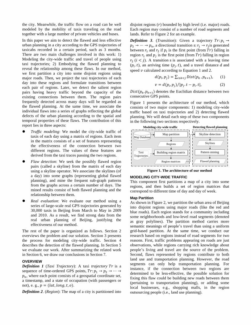
Figure 1 presents the architecture of our method, which
consists of two major components: 1) modeling city-wide
traffic based on taxi trajectories and 2) detecting flawed
planning. We will detail each step of these two components
in the following two sections respectively.
Figure 1. The architecture of our method
MODELING CITY-WIDE TRAFFIC
This component first partitions a map of a city into some
regions, and then builds a set of region matrices that
correspond to different time of day and day of week.
Map Partition
As shown in Figure 2, we partition the urban area of Beijing
into disjoint regions using major roads (like the red and
blue roads). Each region stands for a community including
some neighborhoods and low-level road segments (denoted
as gray polylines). The partition method carries more
semantic meanings of people’s travel than using a uniform
grid-based partition. At the same time, we conduct our
research based on regions instead of road segments for two
reasons. First, traffic problems appearing on roads are just
observations, while regions carrying rich knowledge about
people’s living and travel are the source of the problem.
Second, flaws represented by regions contribute to both
land use and transportation planning. However, the road
segments can only help transportation planning. For
instance, if the connection between two regions are
determined to be less-effective, the possible solution for
fixing this flaw could be building new roads between them
(pertaining to transportation planning), or adding some
local businesses, e.g., shopping malls, in the region
outsourcing people (i.e., land use planning).
Taxi
Trajectories
Region matrices
Map DatabaseMap partition
Building region matrix
Regions
Skyline detection
Pattern mining
Flawed planning
Modeling city-wide traffic Detecting flawed planning
Skylines

Here, we employ Connected Components Labeling (an
image segment method) [11] to segment a map into regions
effectively and efficiently, as the problem of subdivisions in
a polygonal region is NP-complete.
Figure 2. Heat map of the partitioned regions in Beijing
Building Region Matrix
This process is comprised of the following three steps.
1) Temporal partition: In this step, we first partition the taxi
trajectories into two parts according to workday and rest
day (consisting of weekends and public holidays) since
people’s travel on these two types of days are different.
Then, we further segment time of day into some slots in
terms of the traffic conditions in the city.
First, in the same time slot, the traffic conditions and the
semantic meaning of people’s travel are similar. For
example, Figure 3 A) shows the average travel speed of all
the taxis (with passengers) in Beijing at different times of
workdays. The average travel speed of the entire city of
Beijing as defined previously in time slot 7:00-10:30am is
lower than that of the entire day. This matches the generally
accepted assumption that people are going to work during
the morning rush hours. Likewise, the time slot of 4pm-
7:30pm corresponds to the evening rushing hour in the
workday when people go home. Second, if we do not
respectively explore the trajectories from different time
slots, we will miss some actually flawed planning as the
detected results could be dominated by some regions only
having heavy traffic in a particular time slot. Third, the time
partition enables us to explore the temporal relations
between the results detected from continuous time slots,
helping us deeply understand the flaws. We will further
justify the temporal partition later.
A) Workday B) Rest day
Figure 3. Traffic conditions in Bejing changing over time
According to Figure 3, we obtain the time slots shown in
Table 1. Later, we build a region matrix for each time slot
of each day (refer to the following paragraphs).
Time Work day Rest day
Slot 1 7:00am-10:30am 9:00am-12:30pm
Slot 2 10:30am-4:00pm 12:30pm-7:30pm
Slot 3 4:00pm-7:30pm 7:30pm-9:00am
Slot 4 7:30pm-7:00am
Table 1. Time partition for workdays and rest days
2) Transition construction: We pick out the effective trips
with passengers from taxi trajectories in terms of the
occupancy state associated with a sample (a weight sensor
is embedded in a taxi to detect whether there are additional
persons beside a driver in the taxi). So, an effective taxi
trajectory represents a passenger’s trip. Then, we project
these trajectories onto the map and construct transitions
between two regions according to definition 3. As
demonstrated in Figure 4, two trajectories, and ,
respectively traversing and , formulate
four transitions: , , , and ,
denoted as the blue arrows. Note that, a trajectory
discontinuously traversing two regions, such as in
, still formulate a transition between the two regions.
The distance of this transition is ∑ ,
and the travel speed is approximately .
Figure 4. Transfer a trajectory into transitions
Definition 4 (Region Pair). A region pair is a pair of
regions having a set of transitions (between
them). By aggregating the transitions, each region pair is
associated with the following three features: 1) volume of
traffic between these two regions, i.e., the count of
transitions , and 2) expectation of these transitions’
speeds , and 3) ratio between the expectation of the
actual travel distance and the Euclidian distance
between the centroids of two regions, .
∑
, (3)
∑
, (4)
⁄ , (5)
Where is the collection of transitions between and .
Figure 5 plots the region pairs from a time slot 7-10:30am
in a workday in the space. A black point
represents a region pair. The projections of these region
pairs on XZ and YZ spaces are also visualized with green
and blue plots. Note that the value of a given could be
smaller than 1 as taxis might cross two adjacent regions
with a distance shorter than that between the two centroids.
Some might be concerned with the transitions generated by
the trajectories discontinuously passing two regions, e.g.,
8:0
0
10
:00
12
:00
14
:00
16
:00
18
:00
20
:00
22
:00
24
26
28
30
32
34
36
38
40
42
Sp
ee
d (
km
/h)
Time of day
Speed
Average Speed
8:0
0
10:0
0
12:0
0
14:0
0
16:0
0
18:0
0
20:0
0
22:0
0 --
28
30
32
34
36
38
40
42
44
46
48
Sp
ee
d (
km
/h)
Time of day
Speed
Average Speed
p2
Tr2
Tr1
p1
p6
p3
r1
r2
r3p4 p7
p0
p8
r1 r2 r3
r1 r3Tr1:
Tr2:p5

traveling from to in Figure 4, in which a taxi
visited several other regions before reaching . We can
analyze this problem from two perspectives. First, the
connectivity of the two regions should be represented by all
the possible routes between them instead of the fast (or
direct) transitions. Sometimes, reaching a region through a
roundabout route passing other regions is also a good
choice to avoid traffic jams. Second, these discontinuous
transitions do not bias the and . If there is an
effective shortcut between two regions (e.g., ), most
taxis intending to travel from to will still take the
shortcut instead of the roundabout route. That is, the mount
of discontinuous travel is only a small portion in the
transition set. As a result, and are still close to the
real travel speed and ratio that people could travel from to
. On the contrary, if all the taxis have to reach by
passing additional regions, e.g., , that means the route
directly connecting and is not very effective.
Figure 5. Distribution of region pairs in the workday
3) Build region matrix: We formulate a matrix of regions ,
as demonstrated in Figure 6, for each time slot in each day.
An item in the matrix is a tuple, ,
denoting the number of transitions, expectation of travel
speed, and between region and . Supposing there are
workdays and rest days, matrices will be built
if using the scheme of the time slots shown in Table 1.
Figure 6. Region matrix and the properties of each item
DETECTING FLAWED URBAN PLANNING
We first detects the skyline of each region matrix in terms
of the values of each tuple. Then, we mine graph patterns
representing flawed planning from these skylines.
Skyline Detection
will model the connectivity and the traffic
between two regions. Specifically, captures the geometric
property of the connection between a pair of regions. A
region pair with a big means people have to take a long
detour traveling from one region to the other. and represent the features of traffic. A big and small
imply heavy traffic carried by the existing routes between
two regions. In this step, we aim to retrieve the region pairs
with a big , small and large , which indicate
flawed urban planning.
We first select the region pairs having the number of
transitions above the average from a matrix . Then, we
find the skyline set from these selected region pairs
according to and , using skyline operator [1].
Definition 5. (Skyline): The skyline is defined as those
points which are not dominated by any other point. A point
dominates another point if it is as good or better in all
dimensions and better in at least one dimension.
Specifically, in our application, each is not
dominated by others, , in terms of
and . That is, there is no region pair having a
lower speed and bigger than . Figure 7 A) depicts
an example of the skyline set using a blue dash line where
a point denotes a region pair. Clearly, no blank points
simultaneously have a smaller and bigger than the
points from the .
Figure 7. An example of skyline detection
Figure 7 B) shows the process for seeking the skyline. For
example, point 1 does not pertain to the skyline because it is
dominated by point 2. However, point 2 does not dominate
point 3 as point 3 has a bigger than point 2. Likewise,
point 5 and 8 are detected as the skyline while point 4, 6,
and 7 are dominated by the skyline.
The detected skyline is comprised of three kinds of region
pairs. 1) A region pair with a very small and ,
illustrated in Figure 8 A). This means two regions are
connected with some direct routes while the capacity of
these routes are not sufficient as compared to the existing
traffic between the two regions. The small and also
indicate that people have no other choice (even if it is a
detour) but to take these ineffective routes for traveling
between the two regions. Otherwise, the will become
bigger. 2) A region pair with a small and big ,
shown in Figure 8 B). This denotes that people have to take
detours for travelling between two regions while these
010
2030
4050
6070
0
200
400
600
800
1000
-1
0
1
2
34
|S|
E(V) (km/h)
r0 r1 rj rnrn-1
r0
r1
ri
rn
rn-1
ai,jai,1
an,0
a0,1
a1,0
a0,n
a1,n
an-1,0 an-1,n
ai,nai,0M =
ɵ
E(V
)
E(V) ɵ24 1.6
20 2.4
30 2.8
22 2.0
18 1.4
34 2.4
30 2.0
36 3.2
skyline
A) A skyline B) Seeking a skyline
point
1
2
3
4
5
6
7
8

detours suffer from heavy traffic leading to a slow speed.
This is the worst case among these three situations. 3) A
region pair with a big and big , depicted in Figure 8
C). These two values imply that people travel between two
regions by taking some far detours which are fast, e.g., a
high way. Though the speed is not slow, the long distance
will cost people a lot of time and gas. So, the connectivity
between such kinds of regions still has flaws.
Figure 8. Three kinds of region pairs in a skyline
Note that we focus on finding the most salient flawed urban
planning instead of all the poor ones. Seeking the skyline
from the region pairs with a large volume of traffic ( is
above the average), we guarantee 1) the detected skyline is
related to many people’s travel and 2) each ( , ) is
calculated based on a large number of observations.
Pattern Mining from Skylines
In this step, we first build a skyline graph for each day by
connecting the region pairs in the skylines of different time
slots. Then, we detect the sub-graph patterns from these
graphs using a graph pattern mining algorithm [13].
1) Formulating skyline graphs: As demonstrated in Figure 9,
there is a skyline in each time slot (denoted as a row) of
each day (represented by a column). Two region pairs from
two consecutive slots are connected if they are spatially
close to each other. For example, in Day 1 we connect the
region pair from slot 1 to from slot 2,
because these two region pairs share the same node and
appear in the consecutive time slots of the same day.
Likewise, to from these two slots are
connected. However, from slot 1 and
from slot 3 cannot be connected as they are not temporally
close. The built skyline graphs are shown in the fourth
column. Note that, there could be multiple isolated graphs
pertaining to a day like day 2.
2) Mining frequent sub-graph patterns: We mine the
frequent sub-graph patterns from the skyline graphs
across a certain number of days for two reasons. One is to
avoid any false alteration. Sometimes, a region pair with
effective connectivity could be detected as a part of skyline
because of some anomaly events, such as traffic accidents.
The other is to provide a deeper understanding of the
flawed planning. By associating individual region pairs, we
can find the causality and relation among these regions,
which is more valuable for understanding how a problem is
derived. The bottom of Figure 9 shows the mined skyline
patterns using different supports. Here, the support of a sub-
graph pattern is calculated as Equation 6, where is a
skyline graph containing the sub-graph and is the
collection of skyline graphs across days. The denominator
denotes the number of days that the dataset across.
, (6)
For instance, the support of is 1 since it appears
in the skyline graphs of all three days while that of is 2/3 as it only appears in Day 2 and Day 3. Given a
threshold we can choose the patterns with the support .
These patterns represent the flawed urban planning which is
salient and appears frequently.
Figure 9. Mining frequent skyline patterns
Besides, we mine the association rules among these patterns
according to Equation 7 and 8 where denotes the
number of days that and co-occurred and means
the number of days having . Two patterns formulate an
association rule, denoted as , if the support of
and its confidence (a given threshold).
, (7)
. (8)
For example, as depicted in Figure 9, whose support is 2/3 and confidence is 2/3, while the
confidence of is 1.
The mined association rules can consist of over 2 patterns.
For instance, , i. e., has a very high
probability (conditioned by and ) to occur when and
appear simultaneously. Meanwhile, these association
rules may not be geospatially close to each other, hence
revealing the causality and correlation between the flawed
planning that seems to have no relationship in the geo-
spaces. The experiments include more examples.
EVALUATION
Settings
In this section, we carry out our method with a large-scale
taxi trajectory dataset generated in Beijing in the past two
years, and evaluate the detected results based on the real
urban planning published by the government of Beijing.
r1 r2r1 r2 r1 r2
A) E(V)↓, ɵ↓ B) E(V)↓, ɵ↑ C) E(V)↑, ɵ↑
Day 1 Day 2 Day 3
Slo
t 1
Slo
t 2
Sk
yli
ne
Gra
ph
s
r1 r2 r4
r5r3
r2 r8
r5 r7
r8
r4r9
r1 r2
r3
r8
r4
r9
r5 r7
r3
r1 r2
r4 r5
r2
r5 r8
r8
r4
r3
r6
r1 r2 r5r8
r4
r3 r6
r1 r2
r4 r5
r2
r4 r8
r4
r3
r8
r1 r2
r4
r5
r3
r8
r6
Slo
t 3
r1 r2 r8 r4
r4 r5
Support=1.0 Support=2/3
r1 r2 r8 r5r4
r3 r8 r4 r3 r6Patt
ern
s
r2
Ste
p (1
)
Step (2)
Bu
ildin
g sk
ylin
e gra
ph
s
Mining skyline patterns
r4
Taxi trajectories: Table 2 shows the properties of the two
trajectory datasets that we used for evaluating our method.
We select the data from the same time span within a year in
case people have different travel patterns in different
seasons. The latter is slightly larger and denser as some
expired taxis are replaced by new taxis with better facilities.
Datasets 2009. 3-5 2010.3-6
Number of taxis 29,286 30,121
Effective days 89 116
Number of
points
Total 679M 1,730M
Per taxi/day 306 528
Distance
(KM)
Total 310M 600M
Per taxi/day 128 171
Average sampling rate (s) 100 74
Ave. dist. between two points (m) 457 349
Table 2. Two datasets of taxi trajectories used for evaluation
Map data: We use the road network data of Beijing, which
has 106,579 road vertices and 141,380 road segments. We
pick out 25,262 major road segments with level 0, 1, and 2
(0 is the highest level representing highways, 6 is the lowest
denoting small streets) to partition the urban area of Beijing
into some regions. As a result, we obtain 444 regions.
We verify the detected flaws in the following two ways:
1) We select some urban planning, such as new subway
lines and roads, which has been implemented for use
between the times of the two datasets, and study whether
the carried out planning reduces the flaws existing in the
former dataset.
2) We check if some flaws that have been detected in both
two datasets by our method embodied in the future urban
planning of Beijing (i. e., the problem of these regions has
been recognized by the city planner).
We compare our approach with a baseline method which
retrieves the top hottest regions in Beijing according to the
following metric , where denotes the road segments
falling in the region .
∑ ; (9)
This metric represents the density of taxis sending people to
a region in a unit time slot (hour). Here, the total length of
road (in a region) makes more sense beyond the area size of
the region since the length (and capacity) of roads reflect
the real spaces that vehicles can travel. Meanwhile, we do
not differentiate the capacities of the road segments in a
region any longer as all of them are local streets. We will
show the heat maps of Beijing in terms of this metric later.
Results
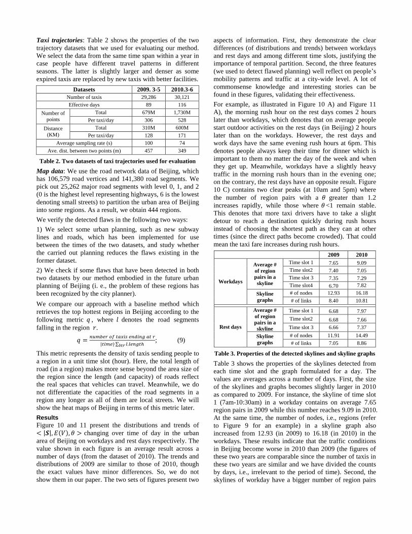
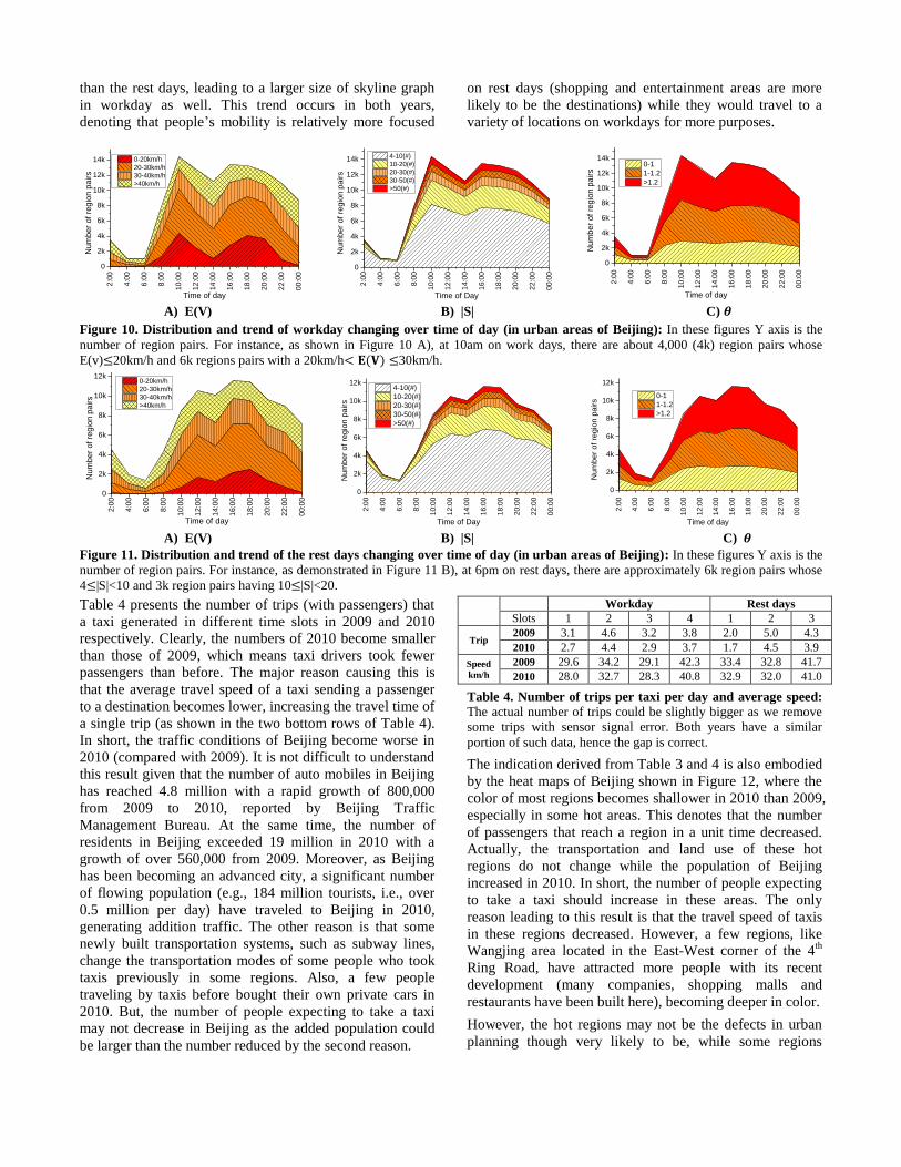
Figure 10 and 11 present the distributions and trends of
changing over time of day in the urban
area of Beijing on workdays and rest days respectively. The
value shown in each figure is an average result across a
number of days (from the dataset of 2010). The trends and
distributions of 2009 are similar to those of 2010, though
the exact values have minor differences. So, we do not
show them in our paper. The two sets of figures present two
aspects of information. First, they demonstrate the clear
differences (of distributions and trends) between workdays
and rest days and among different time slots, justifying the
importance of temporal partition. Second, the three features
(we used to detect flawed planning) well reflect on people’s
mobility patterns and traffic at a city-wide level. A lot of
commonsense knowledge and interesting stories can be
found in these figures, validating their effectiveness.
For example, as illustrated in Figure 10 A) and Figure 11
A), the morning rush hour on the rest days comes 2 hours
later than workdays, which denotes that on average people
start outdoor activities on the rest days (in Beijing) 2 hours
later than on the workdays. However, the rest days and
work days have the same evening rush hours at 6pm. This
denotes people always keep their time for dinner which is
important to them no matter the day of the week and when
they get up. Meanwhile, workdays have a slightly heavy
traffic in the morning rush hours than in the evening one;
on the contrary, the rest days have an opposite result. Figure
10 C) contains two clear peaks (at 10am and 5pm) where
the number of region pairs with a greater than 1.2
increases rapidly, while those where <1 remain stable.
This denotes that more taxi drivers have to take a slight
detour to reach a destination quickly during rush hours
instead of choosing the shortest path as they can at other
times (since the direct paths become crowded). That could
mean the taxi fare increases during rush hours.
2009 2010
Workdays
Average #
of region
pairs in a
skyline
Time slot 1 7.65 9.09
Time slot2 7.40 7.05
Time slot 3 7.35 7.29
Time slot4 6.70 7.82
Skyline
graphs
# of nodes 12.93 16.18
# of links 8.40 10.81
Rest days
Average #
of region
pairs in a
skyline
Time slot 1 6.68 7.97
Time slot2 6.68 7.66
Time slot 3 6.66 7.37
Skyline
graphs
# of nodes 11.91 14.49
# of links 7.05 8.86
Table 3. Properties of the detected skylines and skyline graphs
Table 3 shows the properties of the skylines detected from
each time slot and the graph formulated for a day. The
values are averages across a number of days. First, the size
of the skylines and graphs becomes slightly larger in 2010
as compared to 2009. For instance, the skyline of time slot
1 (7am-10:30am) in a workday contains on average 7.65
region pairs in 2009 while this number reaches 9.09 in 2010.
At the same time, the number of nodes, i.e., regions (refer
to Figure 9 for an example) in a skyline graph also
increased from 12.93 (in 2009) to 16.18 (in 2010) in the
workdays. These results indicate that the traffic conditions
in Beijing become worse in 2010 than 2009 (the figures of
these two years are comparable since the number of taxis in
these two years are similar and we have divided the counts
by days, i.e., irrelevant to the period of time). Second, the
skylines of workday have a bigger number of region pairs
than the rest days, leading to a larger size of skyline graph
in workday as well. This trend occurs in both years,
denoting that people’s mobility is relatively more focused
on rest days (shopping and entertainment areas are more
likely to be the destinations) while they would travel to a
variety of locations on workdays for more purposes.
A) E(V) B) |S| C)
Figure 10. Distribution and trend of workday changing over time of day (in urban areas of Beijing): In these figures Y axis is the
number of region pairs. For instance, as shown in Figure 10 A), at 10am on work days, there are about 4,000 (4k) region pairs whose
E(v) 20km/h and 6k regions pairs with a 20km/h 30km/h.
A) E(V) B) |S| C)
Figure 11. Distribution and trend of the rest days changing over time of day (in urban areas of Beijing): In these figures Y axis is the
number of region pairs. For instance, as demonstrated in Figure 11 B), at 6pm on rest days, there are approximately 6k region pairs whose
4 |S|<10 and 3k region pairs having 10 |S|<20.
Table 4 presents the number of trips (with passengers) that
a taxi generated in different time slots in 2009 and 2010
respectively. Clearly, the numbers of 2010 become smaller
than those of 2009, which means taxi drivers took fewer
passengers than before. The major reason causing this is
that the average travel speed of a taxi sending a passenger
to a destination becomes lower, increasing the travel time of
a single trip (as shown in the two bottom rows of Table 4).
In short, the traffic conditions of Beijing become worse in
2010 (compared with 2009). It is not difficult to understand
this result given that the number of auto mobiles in Beijing
has reached 4.8 million with a rapid growth of 800,000
from 2009 to 2010, reported by Beijing Traffic
Management Bureau. At the same time, the number of
residents in Beijing exceeded 19 million in 2010 with a
growth of over 560,000 from 2009. Moreover, as Beijing
has been becoming an advanced city, a significant number
of flowing population (e.g., 184 million tourists, i.e., over
0.5 million per day) have traveled to Beijing in 2010,
generating addition traffic. The other reason is that some
newly built transportation systems, such as subway lines,
change the transportation modes of some people who took
taxis previously in some regions. Also, a few people
traveling by taxis before bought their own private cars in
2010. But, the number of people expecting to take a taxi
may not decrease in Beijing as the added population could
be larger than the number reduced by the second reason.
Workday Rest days
Slots 1 2 3 4 1 2 3
Trip 2009 3.1 4.6 3.2 3.8 2.0 5.0 4.3
2010 2.7 4.4 2.9 3.7 1.7 4.5 3.9
Speed
km/h
2009 29.6
4
34.2
6
29.1
8
42.3
7
33.4
5
32.8
4
41.7
6 2010 28.0
0
32.7
2
28.3
4
40.8
0
32.9
2
32.0
6
41.0
7 Table 4. Number of trips per taxi per day and average speed: The actual number of trips could be slightly bigger as we remove
some trips with sensor signal error. Both years have a similar
portion of such data, hence the gap is correct.
The indication derived from Table 3 and 4 is also embodied
by the heat maps of Beijing shown in Figure 12, where the
color of most regions becomes shallower in 2010 than 2009,
especially in some hot areas. This denotes that the number
of passengers that reach a region in a unit time decreased.
Actually, the transportation and land use of these hot
regions do not change while the population of Beijing
increased in 2010. In short, the number of people expecting
to take a taxi should increase in these areas. The only
reason leading to this result is that the travel speed of taxis
in these regions decreased. However, a few regions, like
Wangjing area located in the East-West corner of the 4th
Ring Road, have attracted more people with its recent
development (many companies, shopping malls and
restaurants have been built here), becoming deeper in color.
However, the hot regions may not be the defects in urban
planning though very likely to be, while some regions
2:0
0
4:0
0
6:0
0
8:0
0
10
:00
12
:00
14
:00
16
:00
18
:00
20
:00
22
:00
00
:00
0
2k
4k
6k
8k
10k
12k
14k
Nu
mb
er
of
regio
n p
air
s
Time of day
0-20km/h
20-30km/h
30-40km/h
>40km/h
2:0
0
4:0
0
6:0
0
8:0
0
10
:00
12
:00
14
:00
16
:00
18
:00
20
:00
22
:00
00
:00
0
2k
4k
6k
8k
10k
12k
14k
Num
ber
of
regio
n p
air
s
Time of Day
4-10(#)
10-20(#)
20-30(#)
30-50(#)
>50(#)
2:0
0
4:0
0
6:0
0
8:0
0
10
:00
12
:00
14
:00
16
:00
18
:00
20
:00
22
:00
00
:00
0
2k
4k
6k
8k
10k
12k
14k
Num
ber
of
regio
n p
air
s
Time of day
0-1
1-1.2
>1.2
2:0
0
4:0
0
6:0
0
8:0
0
10
:00
12
:00
14
:00
16
:00
18
:00
20
:00
22
:00
00
:00
0
2k
4k
6k
8k
10k
12k
Nu
mb
er
of
regio
n p
air
s
Time of day
0-20km/h
20-30km/h
30-40km/h
>40km/h
2:0
0
4:0
0
6:0
0
8:0
0
10
:00
12
:00
14
:00
16
:00
18
:00
20
:00
22
:00
00
:00
0
2k
4k
6k
8k
10k
12k
Num
ber
of
regio
n p
air
s
Time of Day
4-10(#)
10-20(#)
20-30(#)
30-50(#)
>50(#)
2:0
0
4:0
0
6:0
0
8:0
0
10
:00
12
:00
14
:00
16
:00
18
:00
20
:00
22
:00
00
:00
0
2k
4k
6k
8k
10k
12k
Nu
mb
er
of
regio
n p
air
s
Time of day
0-1
1-1.2
>1.2
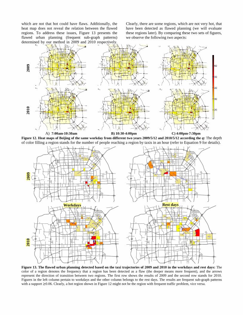
which are not that hot could have flaws. Additionally, the
heat map does not reveal the relation between the flawed
regions. To address these issues, Figure 13 presents the
flawed urban planning (frequent sub-graph patterns)
determined by our method in 2009 and 2010 respectively.
Clearly, there are some regions, which are not very hot, that
have been detected as flawed planning (we will evaluate
these regions later). By comparing these two sets of figures,
we observe the following two aspects:
A) 7:00am-10:30am B) 10:30-4:00pm C) 4:00pm-7:30pm
Figure 12. Heat maps of Beijing of the same workday from different two years 2009/5/12 and 2010/5/12 according the : The depth
of color filling a region stands for the number of people reaching a region by taxis in an hour (refer to Equation 9 for details).
Figure 13. The flawed urban planning detected based on the taxi trajectories of 2009 and 2010 in the workdays and rest days: The
color of a region denotes the frequency that a region has been detected as a flaw (the deeper means more frequent), and the arrows
represent the direction of transition between two regions. The first row shows the results of 2009 and the second row stands for 2010.
Figures in the left column pertain to workdays and the other column belongs to the rest days. The results are frequent sub-graph patterns
with a support 0.06. Clearly, a hot region shown in Figure 12 might not be the region with frequent traffic problem, vice versa.
20
09
20
10
20
10
20
09
Workdays Rest days
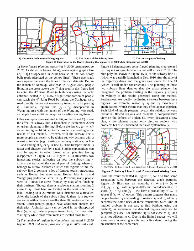
A) New roads built around Wangjing area B) The launch of the Subway line 4 C) The central part of Beijing
Figure 14 Illustration on the flawed planning that appeared in 2009 while disappearing in 2010
1) Some flawed planning occurring in 2009 disappeared in
2010. As shown in Figure 14 A), some region graphs like
disappeared in 2010 because of the two newly
built roads (depicted as the yellow lines). These two roads
were opened between the times of the two datasets. Before
the launch of Nanhuqu west road in August 2009, people
living in the areas above the 4th
ring road in this figure had
to enter the 4th
Ring Road (a high way) using the only
entrance located in . Now, a significant portion of people
can reach the 4th
Ring Road by taking the Nanhuqu west
road directly; hence not necessarily travel to by passing
. Similarly, regions like disappeared in
Wangjing area with the launch of the Wangjing west road,
as people have additional ways for traveling among them.
Other examples demonstrated in Figure 14 B) and C) reveal
the effect of subway line 4 (launched in September 2009)
on urban planning in Beijing. Before the launch,
shown in Figure 14 B) had traffic problems according to the
results of our method. However, with the subway line 4
more people can reach by taking subway systems with a
one-stop transfer (e.g., starting at subway station in line
10 and ending at or in line 4). This transport mode is
faster and cheaper than by a taxi. Similar explanations can
also be applied to other flawed urban planning having
disappeared in Figure 14 B). Figure 14 C) illustrates two
interesting stories, reflecting on how the subway line 4
affects the traffic of the central part of Beijing, where
belongs to central business district and regions within the
subway line 2 contains a lot of famous tourist attractions,
such as Houhai bar street along Houhai lake in and
Wangfujing pedestrian street in . Previous, many people
went to Houhai bar street from by taxis after finishing
their business. Though there is a subway station on line 2
close to , most bars are located in the west side of the
lake, leading to a 20-minute walk distance to a traveler.
After the launch of the subway line 4, there is a subway
station with a distance smaller than 500 meters to the bar
street. Consequently, people have additional choices for
their trips. A similar story can be found in the disappeared
flaw , where people travel to for diner after
visiting while most restaurants are located close to .
2) The number of regions having defects increased in 2010
beyond 2009 and some flaws occurring in 2009 still exist.
Figure 15 demonstrates some flawed planning (represented
by frequent sub-graph patterns) that still exists in 2010. The
blue polyline shown in Figure 15 A) is the subway line 15
(which was partially launched in Dec. 2010 after the time of
the trajectory data), and the green one stands for line 14
(which is still under construction). The planning of these
two subway lines denotes that the urban planner has
recognized the problem existing in the regions, justifying
the validity of the results generated using our method.
Furthermore, we specify the linking structure between these
regions. For example, region , and formulate a
graph pattern, which means that they often appear together.
Such kind of graph patterns reveals the relation between
individual flawed regions and presents a comprehensive
view on the defects of a plan. So, when designing a new
plan, a city planner cannot only discover regions with
problems but also understand the flaws systematically.
Figure 15. Subway Lines 14 and 15 and related existing flaws
From the result presented in Figure 13, we also find some
association rules between the detected graph patterns.
Figure 16 illustrates an example, , ] with support=0.05 and confidence=0.7. In
short, and have a probability of 0.7 to
appear if occurs. This pattern suggests that many
people leaving are heading to regions and while
becomes the bottle-neck of these transitions. Such kind of
implied problem is not easy to find (without using our
method), as sometimes the detected regions may not be
geospatially close. For instance, is not close to , and
is not adjacent to . Due to the limited spaces, we will
show more interesting results and a live demo during the
presentation at the conference.
The 4th
ring road Entrance
Nan
hu
qu
west
Ro
ad
r1r2
Wan
gjin
g w
est
Ro
ad
r3
r4
Subway line 4
Subway line 10
r1
r2
r3
r4
s1
s2
s3
s4
<500m
Subway line 1
Subway line 2
Su
bw
ay
lin
e 4
r2
r1
r3
r4
s1
s2
s3
s4
s5 s6
A) overview B) Line 14 and 15 in Wangjing C) Line 14 passing New CBD
Su
bw
ay
lin
e 1
5
Sub
way
line
14
Su
bw
ay
Lin
e 1
4
r2
r1
Su
bw
ay
lin
e 1
4
r3

Figure 16. Association rules mined from the data of 2010
RELATED WORK
Mining Taxi Trajectories
A significant number of published documents have
presented work aiming to mine the trajectories of taxicabs
since the trajectory data has recently become widely
available. They [5][10] studied taxi drivers’ pick-up
behavior in creating higher profit (e.g., how to easily find
passengers) by analyzing fleet trajectories. Paper [16]
presents some probabilistic models predicting a driver's
destination and route based on historical GPS trajectories.
Paper [6] estimates the real-time traffic flows on some road
segments in terms of the recently received taxi trajectories.
Yuan et al. [14][15] learn the practical, driving path to a
destination from taxi trajectories, considering that taxi
drivers are experienced drivers. Different from the above-
mentioned work, we mine taxi trajectories for supporting
urban planning instead of for an end user. We are the first
team to carry out such studies for this purpose.
Urban Computing
The advances of ubiquitous computing technology have
brought considerable attention to urban computing in recent
years [7][12]. Most literature discusses the urban computing
from the perspective of social computing in the urban area,
e.g., estimating the similarity between users in terms of
their location histories [2][3][9], extracting social structures
from mobile phone data [4], enabling friend and location
recommenders in the real world [17][18], and studying the
influence of pervasive systems on people in urban spaces
[8]. Different from these studies, we explore the urban
computing from the perspective of urban planning, sensing
people’s mobility in a city unobtrusively with taxis and
detect flaws with implicit engagement of citizens.
CONCLUSION
In this paper, we detect the flaws in the existing urban
planning of a city using the GPS trajectories of taxis
traveling in the urban areas. The detected results are
comprised of two sets of findings. One is the frequent sub-
graph patterns consisting of region pairs with salient traffic
problems and the linking structure among these regions.
The other is the association relations between these patterns.
These results can first evaluate the effectiveness of the
carried urban planning, and second provide a
comprehensive view on the existing problem for decision-
making when city planners conceive future plans. We
executed our method based on real data generated by
30,000 taxis in Beijing in 2009 and 2010, and evaluated the
validity of our results using real urban planning of Beijing,
including the newly built subway lines and roads and city
projects that are still under construction. Some interesting
discoveries are revealed from the data as well.
In the future, we might analyze how the detected flaws are
derived from the existing urban planning by 1) studying the
geographic features of a region, such as the road segments
and points of interests, and 2) the purpose of people’s travel,
e.g., for shopping, sports, work etc.
REFERENCES 1. Börzsönyi, S., Kossmann, D., Stocker, K. The skyline operator.
In Proc. ICDE 2001. IEEE Press: 421-430.
2. Cranshaw, J., Toch, E., Hong, J. Kittur, A., Sadeh, N. Bridging
the gap between the Physical Location and Online Social Networks. In Proc. Ubicomp’10, ACM Press (2010): 119-128.
3. Eagle, N., and Pentland, A. Reality mining: sensing complex
social systems. Personal Ubiquitous Computing, 10, 4 (2006):
255–268.
4. Eagle, N., Montjoye, Y. D., and Bettencourt, L. Community
Computing: Comparisons between Rural and Urban Societies using Mobile Phone Data, IEEE Social Computing, 144-150.
5. Ge, Y., Xiong, H., Tuzhilin, A., Xiao, K., Gruteser M., Pazzani
M. J. An Energy-Efficient Mobile Recommender System. In Proc. KDD 2010, ACM Press (2010): 899-908.
6. Guehnemann A., Schaefer R. P., Thiessenhusen K. U., Wagner
P. Monitoring traffic and emissions by floating car data. Institute of transport studies Australia; 2004.
7. Kindberg, T., Chalmers, M., Paulos, E. Gest editors’
introduction: Urban computing. Pervasive computing. 6, 3 (2007), 18-20.
8. Kostakos V., O’Neill, E. Cityware: Urban computing to bridge
online and real-world social networks. Handbook of Research
on Urban Informatics, 2008.
9. Li, Q., Zheng, Y., Xie, X., Chen, Y., Liu, W., Ma, W.Y.
Mining user similarity based on location history. In Proc. GIS 2008, ACM Press (2008): 1-10.
10. Liu, L., Andris, C., Biderman, A. and Ratti, C. Uncovering
cabdrivers’ behavior patterns from their digital traces. Computers, Environment and Urban Systems, 2010.
11. Rosenfeld, A. Connectivity in digital pictures. Journal of the
ACM (JACM), 17, 1(1970): 146-160.
12. Shklovski, I., Chang, M. F. Urban Computing-Navigating Space and Context. IEEE Computer Society. 39, 9 (2006), 36.
13. Yan, X., and Han, J. Discovery of frequent substructures. Wiley-Interscience, 2007. 99-113
14.Yuan J., Zheng Y., Xie, X., Sun, G. Driving with Knowledge from the Physical World. In Proc. KDD 2011, ACM Press 2011.
15. Yuan J., Zheng Y., Zhang C. Y., Xie, W., Xie, X., Sun, G. and
Huang, Y. T-Drive: Driving Directions Based on Taxi Trajectories. In Proc. GIS 2010. ACM Press (2010), 99-108.
16. Ziebart, B., Maas, A., Dey, A. and Bagnell, J. Navigate like a
cabbie: Probabilistic reasoning from observed context-aware behavior. In Proc. Ubicomp 2008, ACM Press (2008): 322.
17. Zheng, Y., Xie, X. and Ma, W. Y. GeoLife: A Collaborative
Social Networking Service among User, Location and Trajectory. IEEE Date Engineer Bulletin, 33, 2 (2010), 32-40.
18. Zheng, Y., Zhang, L., Ma, Z., Xie, X., and Ma, W. Y.
Recommending friends and locations based on individual
location history. ACM Trans. on the Web, 5, 1 (2011), 1-44.
Th
e 3
rd r
ing
ro
ad
Guomao Bridge
Th
e 4
th r
ing
ro
ad
r2r1
r3
r4