Upper-ocean variability in Drake Passage and the Weddell Seagordy/G_Stephenson_dissertation.pdf · 2012-08-29 · Upper-ocean variability in Drake Passage and the Weddell Sea: Measuring

UNIVERSITY OF CALIFORNIA, SAN DIEGO

Upper-ocean variability in Drake Passage and the Weddell Sea:

Measuring the oceanic response to air-sea and ice-ocean interactions

A dissertation submitted in partial satisfaction of the

requirements for the degree

Doctor of Philosophy

in

Oceanography

by

Gordon Ronald Stephenson, Jr.

Committee in charge:

Sarah T. Gille, Co-ChairJanet Sprintall, Co-ChairJan KleisslRobert PinkelDan RudnickMaria Vernet

2012

Copyright

Gordon Ronald Stephenson, Jr., 2012

All rights reserved.

The dissertation of Gordon Ronald Stephenson, Jr. is

approved, and it is acceptable in quality and form for

publication on microfilm and electronically:

Co-Chair

Co-Chair

University of California, San Diego

2012

iii

DEDICATION

Dedicated to my uncle John Stephenson and to my parents, Gordon

and Liz.

iv

EPIGRAPH

The world is always full of the sound of waves. ... The little fishes, abandoning

themselves to the waves, dance and sing and play, but who knows the heart of the

sea, a hundred feet down? Who knows its depth?

— excerpt from Musashi by Eiji Yoshikawa

v

TABLE OF CONTENTS

Signature Page . . . . . . . . . . . . . . . . . . . . . . . . . . . . . . . . . . iii

Dedication . . . . . . . . . . . . . . . . . . . . . . . . . . . . . . . . . . . . . iv

Epigraph . . . . . . . . . . . . . . . . . . . . . . . . . . . . . . . . . . . . . v

Table of Contents . . . . . . . . . . . . . . . . . . . . . . . . . . . . . . . . . vi

List of Figures . . . . . . . . . . . . . . . . . . . . . . . . . . . . . . . . . . viii

Acknowledgements . . . . . . . . . . . . . . . . . . . . . . . . . . . . . . . . xiv

Vita and Publications . . . . . . . . . . . . . . . . . . . . . . . . . . . . . . xvi

Abstract of the Dissertation . . . . . . . . . . . . . . . . . . . . . . . . . . . xvii

Chapter 1 Introduction . . . . . . . . . . . . . . . . . . . . . . . . . . . . 1

Chapter 2 Seasonal variability of upper ocean heat content in Drake Passage 62.1 Abstract . . . . . . . . . . . . . . . . . . . . . . . . . . . 72.2 Introduction . . . . . . . . . . . . . . . . . . . . . . . . . 72.3 Data . . . . . . . . . . . . . . . . . . . . . . . . . . . . . 10

2.3.1 XBT and XCTD profiles . . . . . . . . . . . . . . 102.3.2 Heat Fluxes . . . . . . . . . . . . . . . . . . . . . 11

2.4 Measures of upper-ocean variability . . . . . . . . . . . . 132.4.1 Mixed-layer depth . . . . . . . . . . . . . . . . . . 142.4.2 Upper-ocean heat content . . . . . . . . . . . . . 17

2.5 Seasonal heating and cooling of the upper ocean . . . . . 202.6 Summary . . . . . . . . . . . . . . . . . . . . . . . . . . 232.7 Acknowledgments . . . . . . . . . . . . . . . . . . . . . . 37

Chapter 3 Interannual variability of upper-ocean heat content in DrakePassage . . . . . . . . . . . . . . . . . . . . . . . . . . . . . . 383.1 Abstract . . . . . . . . . . . . . . . . . . . . . . . . . . . 393.2 Introduction . . . . . . . . . . . . . . . . . . . . . . . . . 393.3 Data . . . . . . . . . . . . . . . . . . . . . . . . . . . . . 42

3.3.1 Temperature transects . . . . . . . . . . . . . . . 423.3.2 Eddy database . . . . . . . . . . . . . . . . . . . 433.3.3 Heat fluxes and wind fields . . . . . . . . . . . . . 443.3.4 Climate indices . . . . . . . . . . . . . . . . . . . 44

3.4 Upper-ocean heat content . . . . . . . . . . . . . . . . . 453.5 Variability due to atmospheric forcing . . . . . . . . . . . 47

vi

3.6 Variability due to eddies and meanders . . . . . . . . . . 523.7 Significant contributors to H400 . . . . . . . . . . . . . . 593.8 Summary and Conclusions . . . . . . . . . . . . . . . . . 593.9 Acknowledgments . . . . . . . . . . . . . . . . . . . . . . 77

Chapter 4 Subsurface melting of a free-floating iceberg in the Weddell Sea 784.1 Abstract . . . . . . . . . . . . . . . . . . . . . . . . . . . 794.2 Introduction . . . . . . . . . . . . . . . . . . . . . . . . . 794.3 Background . . . . . . . . . . . . . . . . . . . . . . . . . 81

4.3.1 Turbulent mixing of meltwater . . . . . . . . . . . 814.3.2 Double-diffusive mixing of meltwater . . . . . . . 82

4.4 Data and Methods . . . . . . . . . . . . . . . . . . . . . 834.5 Water masses of Powell Basin . . . . . . . . . . . . . . . 844.6 Results and Discussion . . . . . . . . . . . . . . . . . . . 85

4.6.1 A meltwater estimate from turbulent processes . . 864.6.2 A meltwater estimate from double-diffusive pro-

cesses . . . . . . . . . . . . . . . . . . . . . . . . . 914.7 Conclusions . . . . . . . . . . . . . . . . . . . . . . . . . 954.8 Acknowledgments . . . . . . . . . . . . . . . . . . . . . . 106References . . . . . . . . . . . . . . . . . . . . . . . . . . . . . 107

vii

LIST OF FIGURES

Figure 2.1: Map of Drake Passage showing the locations of the XBT (blackdots) and XCTD (red Xs) casts. The climatological mean frontalpositions (Orsi et al., 1995) of (from north to south) the Sub-antarctic Front, Polar Front, and Southern Antarctic Circum-polar Current Front are indicated (dashed lines). . . . . . . . . 28

Figure 2.2: Monthly heat flux climatologies for NCEP (red), J-OFURO(blue), and OAFlux (black) over regions north (solid line) andsouth (dashed line) of the climatological position of the PolarFront. Vertical lines indicate the two-sigma standard error of a30-day average. . . . . . . . . . . . . . . . . . . . . . . . . . . . 29

Figure 2.3: (a) A section of temperature (◦C) from XBT casts during aDrake Passage transect 18-23 September 2009. The position ofthe Polar Front is indicated by the dashed magenta line. Mixed-layer depth (MLD) is indicated by the black line. The latitudeof example casts in Figures 2.4 and 2.5 are also indicated (tri-angles). (b) Mixed-layer heat content (solid black) and heatcontent integrated to 400 m (dashed line) for XBT casts fromthe transect in (a). . . . . . . . . . . . . . . . . . . . . . . . . . 30

Figure 2.4: Profiles from XCTD casts collected during the transect shownin Figure 2.3 on 20 September 2009 (a,b,c) near 58.5◦ S, 63.7◦

W and on 19 September 2009 (d,e,f) near 56.5◦ S, 64.1◦ W.Profiles show temperature (◦C, a, d), salinity (psu, b, e), andpotential density (kg m−3, c, f). MLDT is shown by the dashedline (a,b,d,e) and MLDρ is shown by the dash-dot lines (b,c,e,f).Dotted lines show differences in MLDT (a,d) and MLDρ (c,f)after ∆T and ∆ρ are changed by ±10%, respectively. In panels(a) and (c), these lines lie very close to the dashed line indicatingMLDT . Note also that the x-axis scale is different for the upperand lower panels. . . . . . . . . . . . . . . . . . . . . . . . . . 31

Figure 2.5: (a) Cumulative distribution functions (CDFs) of the differencebetween MLDT and MLDρ (i.e. MLDT -MLDρ) and (b) CDFsof the change in MLDT in response to a ± 10% perturbation to∆T for XCTD casts collected in winter (solid line) and summer(dotted line), north (red) or south (blue) of the Polar Front. . . 32

Figure 2.6: Temperature (◦C) profiles with depth (m) taken 10 km and lessthan one hour apart at (a) 57.4◦ S and (b) 57.3◦ S near 64.0◦ W,19 September 2009, during the transect illustrated in Figure 2.2.Mixed-layer depths (MLDT , gray dashed line) of (a) 263 m and(b) 118 m were determined using a 0.2◦ C temperature threshold. 33

viii

Figure 2.7: (a) Standard deviation of heat content in 50-m layers north(solid) and south (dashed) of the Polar Front. (b) The corre-lation of heat content in the shallowest layer (0-50 m, black)and in the deepest layer (750-800 m, blue) with heat content inother layers north (solid) and south (dashed) of the Polar Front.The gray bar indicates correlations that are not significant andthe red dotted line delineates 400 m depth. . . . . . . . . . . . 34

Figure 2.8: (a) HML, mean heat content over the mixed layer and (b) H400,heat content in the upper 400 m of the water column for castsnorth (red) and south (blue) of the Polar Front for 85 XBTtransects are plotted against the median year-day of the cruise.Error bars (gray) represent the standard error of the mean. Asinusoidal annual cycle (dashed lines) is least-squares fit to eachtimeseries. Surface heat fluxes drive an annual cycle in heatcontent (green line, offset by 4 GJ m−2) made by integratingdaily net heat flux anomalies (annual mean removed) from NCEP. 35

Figure 2.9: (a) Amplitude and (b) phase of a sinusoidal annual cycle fitto Hz0

north (solid) and south (dashed) of the Polar Front forvalues of z0 ranging from 50 to 800 m in 50 m increments. (c)The fraction of the variance in Hz0

explained by an annual cyclein heat fluxes. The red dotted line indicates 400 m depth. . . . 36

Figure 3.1: Bathymetric map of Drake Passage showing the locations ofXBTs (black dots). The climatological mean frontal positions(Orsi et al., 1995) of (from north to south) the SubantarcticFront, Polar Front, and Southern Antarctic Circumpolar Cur-rent Front are indicated (dashed lines). . . . . . . . . . . . . . . 62

Figure 3.2: Temperature transects from June cruises in (a) 2006 and (b)2009. Transects of heat content from 0-400 m, h400, across (c)the June 2006 transect and (d) the June 2009 transect withaverage heat content north of the Polar Front (HN , red dottedline), south of the Polar Front (HS, blue dotted line), and overthe entire transect (H400, black dotted line). The latitude ofthe Polar Front is indicated by a magenta line (a,b,c,d). Mapsof daily sea surface height anomaly (e) 12 June 2006 and (f)30 June 2009 and locations of XBT casts (black x). Centerlocation and approximate length scale of cyclonic (blue) andanticyclonic (red) eddies identified in the Chelton et al. (2011b)database. Apparent overlap of eddies may be caused by linearinterpolation of eddy position or by approximation of the eddiesas circular. . . . . . . . . . . . . . . . . . . . . . . . . . . . . . 63

ix

Figure 3.3: Transect-averaged H400 (black x) and an annual cycle fitting anannual and semiannual cycle (red curve). H′

400(black circles)

are the residuals relative to the annual cycle. . . . . . . . . . . 64Figure 3.4: Linear regression red (dotted line) of H′

400onto (a) HN (r =0.506),

(b) HS (r =0.292) and (c) latitude of the Polar Front (φPF , r =-0.599). . . . . . . . . . . . . . . . . . . . . . . . . . . . . . . . . 65

Figure 3.5: (a) A map of the correlation between H′400

and Q′net 75 days

prior (Q75d) shows a maximum near 60oS, 289oE. The intervalbetween contours is 0.05. (b) The correlation between Q′

net at60oS, 289oE and H′

400reaches a maximum at ∼75 days. Positive

time lag indicates Q′net precedes H′

400. . . . . . . . . . . . . . . 66

Figure 3.6: (a) Correlation of NCEP Reanalysis 1 heat flux anomalies (Q′net)

with meridional wind anomalies. (b) Regression coefficients ofQ′

net onto meridional wind anomalies. Climatological positionof the ACC fronts (dashed lines)are, from north to south, theSubantarctic Front, Polar Front, and southern ACC Front. Lo-cations of XBT casts (black dots) are indicated. . . . . . . . . . 67

Figure 3.7: Correlations between the ENSO index (black line) or the SAMindex (blue line) and (a) H′

400, (b)φPF , (c) H′

N , and (d) H′S.

Positive time lags indicate the ENSO or SAM index precedes theXBT transect. Red dotted lines indicate the 0.95 significancelevel. . . . . . . . . . . . . . . . . . . . . . . . . . . . . . . . . . 68

Figure 3.8: (a) Upper-ocean heat content anomalies, h′400

, relative to a sea-sonal cycle and a spatial mean (binned by latitude). The lati-tude of cold-core (blue circle) and warm-core (red circle) eddiesthat intersect an XBT transect are indicated, as well as the lo-cation of the Polar Front (black x) (b) A schematic depictingdetermination of the heat content anomaly associated with atransect crossing an eddy, he. The length, L, of the intersectionbetween a transect (magenta line) and an eddy (black circle)depends on the minimum distance, d, from the center of theeddy to the transect and the length scale, R, of the eddy. . . . . 69

Figure 3.9: Spatial distribution of h′400

in (a) a composite cylonic (cold-core)eddy and (c) a composite anticyclonic (warm-core) eddy. Forheat content measurements near an eddy, values of h′

400were

normalized by the eddy’s amplitude (units are GJ m−2 per cmeddy amplitude) and binned by position relative to the eddycenter. Zonal and meridional displacement from the center ofthe eddy are scaled by the effective length-scale of the eddy. Thestandard error of the bin average is shown for (b) the cycloniceddy and (d) the anticyclonic eddy. Contour intervals are 0.05(a,c) or 0.01 (b,d) GJ m−2 per cm. . . . . . . . . . . . . . . . . 70

x

Figure 3.10: (a) The heat content anomaly associated with the eddy is a func-tion of distance from the eddy center and the length scale andamplitude, A, of the eddy. For measurements located within aneddy, h′

400was normalized by the amplitude of the eddy; binned

averages of h′400

/A were computed at d/R ranging from 0.1 to2. Mean (black line) ± one standard error (dotted lines) andmedian (red) h′

400/A decrease from maxima near 0.3R from the

eddy center to 0 at 1 to 1.3R from the center. A truncatedGaussian curve (blue line) as in equation (3.4) approximatesf(r, A). (b) A scatterplot of h′

400against the value of f(r, A) at

each measurement point (black circles), with a one-to-one linefit (dashed line). . . . . . . . . . . . . . . . . . . . . . . . . . . 71

Figure 3.11: Peak amplitude of the functional fit (black x) computed as forFigure 3.10 for depths between 0 and 600 m. The increasewith depth is approximated by an exponential curve (blue line)described by (0.33 × (1 − ez0/634)). . . . . . . . . . . . . . . . . 72

Figure 3.12: A scatterplot of H′400

against the sum of heat content anomaliesdue to eddies (E). A linear regression (red dashed line) has aslope of 0.80±0.22. Uncertainties in E (gray lines) are computedas discussed in Section 3.7. . . . . . . . . . . . . . . . . . . . . 73

Figure 4.1: (a) Powell Basin is in the northwest Weddell Sea, just east ofDrake Passage and the Antarctic Peninsula, south of the ScotiaSea. (b) C-18a travelled clockwise around the Powell Basin; theestimated positions on March 11 (I), March 22 (II), March 31(III), and April 10 (IV) are indicated. CTD casts were collectednear C-18a on March 10-17 (red), March 18-22 (blue), March 29-April 2 (green), and April 10-11 (magenta). Sampling occurredin Iceberg Alley (IA, orange) April 4-9. Outside of IA, caststhat were more than 50 km from C-18a at the time of surveyare grouped together (cyan) and include casts taken April 3-7at or en route to a reference station (C) and one cast taken∼74 km from C-18a on March 29 (near III). . . . . . . . . . . . 98

Figure 4.2: T-S curves for 56 CTD profiles are grouped by location and timeand color-coded as in Fig. 4.1. CTD casts were collected near C-18a on March 10-17 (red), March 18-22 (blue), March 29-April2(green), April 10-11 (magenta), in Iceberg Alley (orange), andfar from ice (cyan). A seasonal thermocline lies between theAASW and WW. A permanent thermocline separates WW fromWDW. . . . . . . . . . . . . . . . . . . . . . . . . . . . . . . . 99

xi

Figure 4.3: The freezing temperature of seawater (Tfp, solid line at left),temperature (solid) and salinity (dash-dot) profiles with 1 ◦Cand 0.5 psu offsets (left to right) 0.85 km, 2.78 km, 4.63 km,6.48, and 8.96 km west of C-18a collected over a 6-hour periodApril 10-11 (Region IV, magenta in Fig. 4.1b). The WinterWater layer in the cast 0.85 km from C-18a is highlighted in red.100

Figure 4.4: (a) T-S diagrams of casts taken 10-11 April (IV, magenta inFig. 4.1). The cast 0.85 km from C-18a (see Fig. 4.3) showswarm and salty anomalies in the temperature-minimum layer(red). (b) Expanded view of a warm, salty anomaly (i) boundedby points a and b, illustrating the meltwater estimation proce-dure outlined in the text. A point p in the anomaly is modeledas an along-isopycnal mixture of water at d from the meltwa-ter mixing line, L1, and water at e from a linear approximationto the ambient T-S relation, L2. The temperature and salinityrequired for basal melting to produce the anomaly (i) occurswhere L1 intersects the ambient T-S curve at c. Two additionalanomalies (ii and iii) are evident in this cast. . . . . . . . . . . 101

Figure 4.5: (a) The freezing temperature (red line, left) and profiles of tem-perature (red) and potential density (black) in two casts takenone hour apart 0.4 km (left) and 1.4 km (right) south of C-18a,March 22 (blue in Fig. 4.1b). The profile on the right is offset2 ◦C and 0.2 kg m−3. Isopycnals (dotted line) slant upwardsaway from the ice in 50-100 m depth range, so that steps intemperature and potential density in the cast at 0.4 km areevident at the same potential densities in the cast at 1.4 km,shifted vertically by ∼ 12 m. (b) Expanded view of a step intemperature (red), salinity (blue) and potential density (offsetby -992.99 kg m−3) (black) in the cast 0.4 km from C-18a (leftprofile in (a)), illustrating the step-finding procedure outlinedin the text. The interfaces at f and m have lower bounds atg and n, respectively, at depths indicated by the dotted lines.A minimum in ∂σ/∂z is found at q. R is drawn tangent tothe salinity/depth profile at the depths of g and n. The areabetween R and the salinity-depth profile (blue line) defines thesalinity deficit. . . . . . . . . . . . . . . . . . . . . . . . . . . . 102

xii

Figure 4.6: (a) Observed layer thickness (x) and layer thickness predictedfrom equation (4.2) (solid line), calculated from temperatureand salinity data for the profile at 0.4 km in Fig. 4.5a. Layerthickness is at a minimum in the temperature minimum layerand increases below 200 m. (b) Mean observed (red) and pre-dicted (blue) layer thicknesses binned by depth for all layersidentified in potential density profiles. Where layers were ob-served, predicted layer thickness (red) is calculated as the aver-age value of h in equation (4.2) over the depth range of the layer.Black lines indicate standard error. Layer thickness agrees mostclosely in the 40-100 m depth range, averaging about 5 m. . . . 103

xiii

ACKNOWLEDGEMENTS

Working with Sarah Gille and Janet Sprintall has been an honor. I have

benefited greatly from their guidance and their thoughtful and insightful com-

ments. I am grateful for their kindness and dedication, their persistence through

many revisions, and especially for their patience, which has withstood all the tests

I put to it.

I am also thankful for the support of the other members of my committee.

I would like to thank Maria Vernet for her enthusiasm and for introducing me to

the world of icebergs, Dan Rudnick and Rob Pinkel for their guidance as I planned

my research, and Jan Kleissl for his help as I finished my research. I would also

like to thank my former committee member, Paul Linden, for his input on Chapter

IV as it was being prepared.

The help and support of SIO staff has been invaluable. Special thanks go

to Tomomi Ushii and Phil Moses, who have helped me throughout my time at

SIO. Thanks also go to April Fink for helping me with fellowship applications,

to Gilbert Bretado for helping organize my defense, and to the rest of the SIO

graduate office.

My life has been greatly enriched by the support and friendship of my peers.

So thank you to all my mates. My office mates Tamara and Dian, who for years

has been an unending source of chocolate and laughter. My hall mates Jim and

Kyla, who inspired me by the examples they set. A note in the acknowledgments is

insufficient to express thanks for my classmates; San, Yvonne, Peter, Ben, Aneesh,

Mike, James, Shang, and Tom made up much of my day-to-day world, and it

was a good one. I have also been fortunate to have wonderful housemates; thank

you Anais, Jason, James, and Kaushik, for cooking and sharing and late-night

discussions. Thanks also to my shipmates during the iceberg cruise on the N.B.

Palmer, in particular to Ron and John and Maria, who have since been my co-

authors and collaborators. And thanks to my teammates, the Pier Gladiators, for

spending 300 hours of toe-breaking, mind-clearing soccer on the beach.

Finally, thank you to my family for their love and support, and to Claire,

who understands.

xiv

Chapter II, in full, is a reprint with no modifications to content of the article

as it appears in Journal of Geophysical Research-Oceans, 2012, G.R. Stephenson

Jr., S.T. Gille, and J. Sprintall, reproduced with permission of American Geo-

physical Union. The dissertation author was the primary researcher and author of

this manuscript. Janet Sprintall provided the XBT/XCTD data and directed and

supervised the research along with Sarah Gille.

Chapter III, in full, is a manuscript in preparation for publication. I was the

primary researcher and author of this material, with contributions from co-authors

Sarah Gille and Janet Sprintall.

Chapter IV, in its entirety, is a reprint with no modifications to content of

the article as it appears in Deep-Sea Research II, 2011, G.R. Stephenson Jr., J.

Sprintall, S.T. Gille, M. Vernet, J.J. Helly, and R.S. Kaufmann, reproduced with

permission of Elsevier. I was the primary researcher and author of this manuscript.

Maria Vernet, John Helly, and Ron Kaufmann contributed to the field component

of the research which forms the basis of this chapter. Janet Sprintall and Sarah

Gille supervised the analysis and writing of the manuscript.

xv

VITA

2006 B.S., Mathematics and Atmospheric and Oceanic Sciences,University of Wisconsin-Madison

2012 Ph.D., OceanographyScripps Institution of Oceanography,University of California, San Diego.

PUBLICATIONS

Stephenson G.R. Jr., Gille S.T., and J. Sprintall, [in prep]: Interannual variabilityof upper ocean heat content in Drake Passage.

Stephenson G.R. Jr., Gille S.T., and J. Sprintall, 2012: Seasonal variability ofupper ocean heat content in Drake Passage. J. Geophys. Res., 117, C04019.

Stephenson G.R., Sprintall J., Gille S.T., Vernet M., Helly J.J., and R.S. Kauf-mann, 2011: Subsurface melting of a free-floating Antarctic iceberg. Deep-Sea Res.

II., 58(11-12), 1336–1345.

Helly J.J., Kaufmann R.S., Vernet M., and G.R. Stephenson, 2011: Spatial char-acterization of the meltwater field from icebergs in the Weddell Sea. Proc. of the

Nat. Acad. of Sci., 108(14), 5492–5497.

Helly J.J., Kaufmann R.S., Stephenson G.R., and M. Vernet, 2011: Cooling, di-lution and mixing of ocean water by free-drifting icebergs in the Weddell Sea.Deep-Sea Res. II., 58(11-12), 1346–1363.

Gille, S.T., A. Lombrozo, J. Sprintall, G. Stephenson and R. Scarlet, 2009: Anoma-lous spiking in spectra of XCTD temperature profiles. J. Atmos. Ocean. Tech.,26(6), 1157–1164.

Fukumura, K., D. Kazanas, and G. Stephenson, 2009. Quasi-periodic oscillationsfrom random X-ray bursts around rotating black holes. The Astrophysical Journal,695, 1199-1209.

Seemann, S., E. Borbas, R. Knuteson, H.-L. Huang, and G. Stephenson, 2008:Global infrared emissivity for clear sky atmospheric regression retrievals. J. Appl.

Meteorol. Climatol., 47(1), 108–123.

Lehman-Ziebarth, N., P. Heideman, R. Shapiro, S. Stoddart, C. Hsiao, G. Stephen-son, P. Milewski, and A. Ives, 2005: Evolution of Periodicity in Periodical Cicadas.Ecology, 86(12), 3200–3211.

xvi

ABSTRACT OF THE DISSERTATION

Upper-ocean variability in Drake Passage and the Weddell Sea:

Measuring the oceanic response to air-sea and ice-ocean interactions

by

Gordon Ronald Stephenson, Jr.

Doctor of Philosophy in Oceanography

University of California, San Diego, 2012

Sarah T. Gille, Co-ChairJanet Sprintall, Co-Chair

In the first part of this dissertation, reanalysis heat flux products and

profiles from a 15 year time series of high-resolution, near-repeat expendable

bathythermograph / expendable conductivity-temperature-depth (XBT/XCTD)

sampling in Drake Passage are used to examine sources of upper-ocean variability,

with a focus on the nature of MLD variations and their impact on a first-order,

one-dimensional heat budget for the upper ocean in the regions north and south

of the Polar Front. Results show that temperature and density criteria yield dif-

ferent MLD estimates, and that these estimates can be sensitive to the choice of

threshold. The difficulty of defining MLD in low-stratification regions, the large

xvii

amplitude of wintertime MLD (up to 700 m in Drake Passage), and the natural

small-scale variability of the upper ocean result in considerable cast-to-cast vari-

ability in MLD, with changes of up to 200 m over 10 km horizontal distance. In

contrast, the heat content over a fixed-depth interval of the upper ocean shows

greater cast-to-cast stability and clearly measures the ocean response to surface

heat fluxes. In particular, an annual cycle in upper ocean heat content is in good

agreement with the annual cycle in heat flux forcing, which explains 24% of the

variance in heat content above 400 m depth north of the Polar Front and 63% of

the variance in heat content south of the Polar Front. At interannual timescales,

the primary drivers of interannual variations in upper-ocean heat content in Drake

Passage are advective processes; up to 40% of the variance of cross-Passage aver-

age upper-ocean heat content is due to meanders of the Polar Front, while 14%

of the variability results from mesoscale eddies. Heat flux anomalies contribute

less variance (5-10%) on interannual timescales. Teleconnections with ENSO and

SAM contribute to anomalies in meridional winds and heat fluxes. As a result,

ENSO and SAM contribute variability in upper ocean heat content at near-zero

lags; ENSO and SAM are also correlated with upper ocean heat content anomalies

on timescales of ∼2-5 years.

The second part of this dissertation explores a melting iceberg as a source of

upper-ocean variability. Observations near a large tabular iceberg in the Weddell

Sea in March and April 2009 show evidence that water from ice melting below the

surface is dispersed in two distinct ways. Warm, salty anomalies in T-S diagrams

suggest that water from the permanent thermocline is transported vertically as a

result of turbulent entrainment of meltwater at the iceberg’s base. Stepped profiles

of temperature, salinity, and density in the seasonal thermocline are more char-

acteristic of double-diffusive processes that transfer meltwater horizontally away

from the vertical ice face. These processes contribute comparable amounts of

meltwater–O(0.1 m3) to the upper 200 m of a 1 m2 water column–but only basal

melting results in significant upwelling of water from below the Winter Water layer

into the seasonal thermocline. This suggests that these two processes may have

different effects on vertical nutrient transport near an iceberg.

xviii

Chapter 1

Introduction

1

2

As anthropogenic forcing alters atmospheric conditions worldwide, the ef-

fects on the global ocean are mediated by interactions between the atmosphere,

cryosphere, and ocean. The Southern Ocean serves as an entry point for deep-

ocean sequestration of carbon (Caldeira and Duffy, 2000), and Southern Ocean

warming is implicated in the future response of global atmospheric temperatures

to increased radiative forcing associated with increasing atmospheric CO2 concen-

trations (Boe et al., 2009). Predicted changes in Antarctic climate associated with

anthropogenic warming include strengthening of the circumpolar westerly winds

and a southward shift in Southern Ocean storm tracks (Bracegirdle et al., 2008).

Global changes in large-scale atmospheric forcing have been associated with shifts

in the frequency or intensity of climate modes such as El Nino / Southern Oscilla-

tion (ENSO) and the Southern Annular Mode (SAM) (e.g., Meredith et al., 2008),

and significant responses to these modes of atmospheric variability have been seen

in the Southern Ocean (e.g., Meredith et al., 2008; Sprintall, 2008; Sallee et al.,

2008) and in the sea-ice along the coast of Antarctica (e.g., Yuan and Martinson,

2000; Kwok and Comiso, 2002; Sprintall, 2008). The response of the Antarctic

Circumpolar Current (ACC) in particular has been shown to affect global water

mass properties (Naveira Garabato et al., 2009), and the global meridional over-

turning circulation (Wolfe and Cessi, 2010; Marini et al., 2011). The global ocean

heat budget is sensitive to the amount of energy taken up by the Southern Ocean

(see, e.g., Trenberth and Fasullo, 2010; Gille, 2008; Levitus et al., 2009); however,

the remoteness and extreme conditions of the Southern Ocean have led to a histor-

ical scarcity of in situ measurements in the region, and there remains considerable

uncertainty in the basic heat budget of the upper ocean in the region (Dong et al.,

2007). This dissertation examines several different ways to measure the effects

of air-sea or ice-ocean interactions so that we can better identify the mechanisms

that govern upper ocean variability in the Southern Ocean and better predict the

changes that might occur as a result of a changing climate.

One of the primary objectives of Chapter 2 is to identify a robust way to

measure the response of the upper ocean to surface forcing. Mixed-layer depth

(MLD) is commonly used to define the lower limit of direct atmospheric forcing in

3

the ocean, but MLD is also a major source of uncertainty in the Southern Ocean

heat budgets (Dong et al., 2007). The variability of MLD estimates is strongly

affected by oceanic conditions; low stratification and interleaving layers contribute

to high variability north of the Polar Front, while a strong permanent pycnocline

limits MLD variability south of the Polar Front. Thus, MLD is an unreliable

measure of the effects of surface forcing on the upper ocean, as the response of

MLD to a given atmospheric input is inconsistent. A more robust measure of the

response of the upper ocean to atmospheric forcing is found to be the heat content

of the upper ocean over a fixed depth range. Heat content is directly forced by

surface heat fluxes, and results show that on seasonal time scales, a climatological

seasonal cycle in surface heat fluxes is sufficient to explain ∼24% of the variance

in upper ocean heat content above 400 m depth in the region north of the Polar

Front in Drake Passage and ∼63% of the variance in upper ocean heat content in

the region south of the Polar Front in Drake Passage (Stephenson et al., 2012).

Chapter III continues the exploration of upper ocean heat content variabil-

ity in Drake Passage with the goal of identifying the mechanisms governing vari-

ability in upper ocean heat content at interannual time scales. An effort is made

to distinguish between two types of interannual variability: variability governed

by changes in surface forcing on interannual time scales and variability intrinsic

to the ocean, such as frontal meanders and mesoscale eddies. On interannual time

scales, heat flux anomalies upstream of Drake Passage make a small (5-10%) but

significant contribution to upper ocean heat content variability. These heat flux

anomalies are strongly linked to meridional wind anomalies, as other studies have

also shown (e.g., Meredith et al., 2008; Naveira Garabato et al., 2009). Meridional

wind anomalies, in turn, have been linked to ENSO and, in the southeast Pacific,

to SAM (Turner, 2004). The response of upper-ocean heat content in Drake Pas-

sage to ENSO and SAM generally compares favorably with the response of surface

or near-surface temperatures seen in other studies in locations in or near Drake

Passage (Meredith et al., 2008; Sprintall, 2008; Naveira Garabato et al., 2009). The

contribution of mesoscale eddies and frontal meanders to interannual variations in

upper ocean heat content is examined using a database of tracked eddies (Chelton

4

et al., 2011b). Mesoscale variability appears to play a dominant role in governing

upper ocean heat content in Drake Passage; eddies and meanders explain nearly

half of the interannual variability of upper ocean heat content averaged across

Drake Passage. Together, heat fluxes, ENSO variability, mesoscale eddies and

frontal meanders explain ∼84% of the total (seasonal and interannually-varying)

variance in average heat content above 400 m in Drake Passage.

The remainder of the dissertation focuses on ice-ocean interactions. Calving

from glaciers in Antarctica accounts for 2,000 Gt of yearly freshwater input into

the Southern Ocean, half of which takes the form of large tabular icebergs (Jacobs

et al., 1992). Changes in upper ocean temperatures and circulation near the coast

of Antarctica have the potential to rapidly melt ice sheets (Jacobs et al., 2011).

Recent large ice-shelf break-ups, such as the Wilkens Ice Shelf in spring 2009 and

Larsen B in 2002, were followed by an intense period of iceberg spawning. Due

to the potential sea level rise associated with melting of ice shelves and ice sheets,

considerable effort has been undertaken to understand how oceanic conditions and

atmospheric conditions contribute to melting, calving, and ice-shelf break-up (e.g.,

Jacobs et al., 2011). The influence of icebergs on the ocean is less well understood.

Drifting icebergs redistribute heat and freshwater, and transport trace metals and

phytoplankton (Smith et al., 2007). Recent studies have shown that the wake of an

iceberg is associated with an increase in surface chlorophyll concentration (Schwarz

and Schodlok, 2009), and their effect on surface temperature and salinity may affect

rates of sea-ice formation and Antarctic Bottom Water formation (Jongma et al.,

2009). In regions with high iceberg concentrations, such as the Weddell Sea, iceberg

meltwater is a larger term in the freshwater balance than the precipitation minus

evaporation, and large icebergs greater than 10 nautical miles in one dimension

are thought to be responsible for most of the transport of freshwater north of 63◦ S

(Silva et al., 2006). Models that include icebergs often consider them as sources of

surface freshwater(e.g., Jongma et al., 2009). While icebergs do have a net cooling

and freshening effect on the surface ocean (Helly et al., 2011a) over distances of

tens of kilometers (Helly et al., 2011b), they also have a vertical extent of tens to

hundreds of meters. Melting that occurs below the sea surface produces meltwater

5

that can be dispersed in complicated ways.

Chapter IV presents a detailed case study of the effects of one large tab-

ular iceberg on the upper-ocean in the northwest Weddell Sea in March-April

2009. Subsurface melting at the sides and base of an iceberg introduces iron-rich

meltwater to the surrounding ocean in two ways (Stephenson et al., 2011). Double-

diffusive processes at the iceberg’s sidewalls lead to the formation of stepped fea-

tures in temperature and density profiles that may transport meltwater horizon-

tally over tens of kilometers. Meltwater formed at the base of an iceberg appears to

mix turbulently with surrounding Weddell Deep Water, resulting in an injection

of relatively warm, nutrient-rich water to the base of the thermocline, present-

ing possibilities for vertical nutrient transport that may contribute to observed

productivity increases in the wake of large icebergs (Schwarz and Schodlok, 2009).

Chapter 2

Seasonal variability of upper

ocean heat content in Drake

Passage

6

7

2.1 Abstract

Mixed-layer depth (MLD) is often used in a mixed-layer heat budget to

relate air-sea exchange to changes in the near-surface ocean temperature. In this

study, reanalysis heat flux products and profiles from a 15-year time series of

high-resolution, near-repeat XBT/XCTD sampling in Drake Passage are used to

examine the nature of MLD variations and their impact on a first-order, 1-D heat

budget for the upper ocean in the regions north and south of the Polar Front.

Results show that temperature and density criteria yield different MLD estimates,

and that these estimates can be sensitive to the choice of threshold. The difficulty

of defining MLD in low-stratification regions, the large amplitude of wintertime

MLD (up to 700 m in Drake Passage), and the natural small-scale variability of

the upper ocean result in considerable cast-to-cast variability in MLD, with changes

of up to 200 m over 10 km horizontal distance. In contrast, the heat content over

a fixed-depth interval of the upper ocean shows greater cast-to-cast stability and

clearly measures the ocean response to surface heat fluxes. In particular, an annual

cycle in upper-ocean heat content is in good agreement with the annual cycle in

heat flux forcing, which explains ∼24% of the variance in heat content above 400 m

depth north of the Polar Front and ∼63% of the variance in heat content south of

the Polar Front.

2.2 Introduction

The Southern Ocean has experienced statistically significant warming over

the past few decades (Boning et al., 2008; Gille, 2008; Levitus et al., 2009). Warm-

ing of the interior ocean contributes to thermosteric sea level rise (Church et al.,

2011), but heat uptake by the ocean may also act to slow the warming of the

atmosphere associated with anthropogenic forcing (Boe et al., 2009). Intermediate

water properties of much of the world ocean are set by air-sea interactions in the

Southern Ocean (Hanawa and Talley, 2001). In recent decades, Subantarctic Mode

Water and Antarctic Intermediate Water have shown changes consistent with sur-

face warming and increased precipitation in their Southern Ocean source regions

8

(Bindoff and McDougall, 2000; Durack and Wijffels, 2010). Understanding the

rate at which heat is transferred from the atmosphere through the upper layers of

the Southern Ocean will help us better determine the effects of global warming on

both the ocean and the atmosphere.

In many studies of air-sea exchange, the limit of the upper-ocean is defined

to be the mixed layer. The mixed-layer depth (MLD) can be used to relate near-

surface temperature changes to the heat fluxes in and out of the mixed layer (e.g.

Kuhnel and Henderson-Sellers, 1991; Qiu and Kelly, 1993; Dong et al., 2007). In

the Southern Ocean, several mixed-layer depth climatologies have been developed

(e.g. Kara et al., 2003; de Boyer Montegut et al., 2004; Dong et al., 2008; Holte and

Talley, 2009). However, the MLD values in these climatologies differ depending

on the methods (e.g. threshold difference, gradient, hybrid algorithm) (Holte and

Talley, 2009) and parameters (e.g. temperature vs. density) (de Boyer Montegut

et al., 2004) that are used to determine MLD. In the Southern Ocean, weak

stratification or temperature inversions are common (Dong et al., 2008) and may

contribute to the disagreement between estimates of MLD. Differences in Southern

Ocean MLD estimates contribute to uncertainty not only in Southern Ocean heat

budgets (Dong et al., 2007) but in global climate models as well. For example,

MLD differences are a major cause of inter-model spread in the projected rate of

heat transfer to the ocean interior and hence to the projected rate of increase of

globally-averaged surface air temperature in the next 100 years (Boe et al., 2009).

This underscores the importance of determining accurate and reliable estimates of

vertical heat transfer in the Southern Ocean.

In fact, the choice to use MLD as the representative length scale for vertical

mixing of heat within the upper ocean is not obvious. In their seminal paper, Price

et al. (1986) introduced a vertical-mixing model (known as “PWP”) that is now

widely used to study the temporal evolution of the upper ocean, including the

mixed layer. In the same study, Price et al. (1986) acknowledged some limitations

of MLD. Calculating MLD is an attempt to define a quasi-homogeneous layer,

where water properties (often temperature or density) are roughly uniform; the

degree of desired homogeneity can be tuned by requiring that water properties

9

vary by less than a specified amount. When stratification in the upper ocean is

weak, MLD estimates can be sensitive to the specified degree of non-homogeneity.

Price et al. (1986) addressed this limitation and discussed two other vertical length

scales: “trapping depth” is the weighted average depth of the temperature anomaly

above a reference depth; “penetration depth” is a depth derived by relating the

rate of change of near-surface temperature to changes in the upper-ocean heat

content. In the following, we will show that upper-ocean heat content itself can be

a useful measure of ocean uptake of heat from the atmosphere.

Surface forcing is one of the main drivers of upper-ocean variability, pro-

viding the energy input for seasonal cycles in oceanic heating and cooling. A

good measure of upper-ocean variability will reflect the changes in ocean state

corresponding to such forcing; however, other processes can also influence the

upper-ocean. Horizontal advection in the form of eddies and frontal meanders, for

example, can cause a strong warming or cooling signal through the upper 1000 m

of the water column (e.g., Joyce et al., 1981). Vertical entrainment and mixing

within the upper ocean redistribute heat internally and are a source of upper-ocean

variability. To the extent that these processes are occurring in the upper ocean,

the relationship between surface forcing and parameters representing the state of

the upper ocean becomes less immediate and more difficult to discern.

This study will compare the characteristics of several measures of upper-

ocean variability and evaluate their utility as measures of the ocean’s response to

surface heating. We focus on the Drake Passage, where a 15-year time-series of pro-

file data from expendable probes along a near-repeat transect allows estimation of

the seasonal patterns of surface heat forcing and the oceanic response. Section 2.3

describes the upper-ocean data and the heat flux products used in the analysis.

Section 2.4 compares characteristics of MLD and heat content. Section 2.5 relates

seasonal patterns in surface forcing, mixed-layer heat content and upper-ocean

heat content. We present a simplified two-term (temperature tendency and total

heat flux) seasonal heat budget for the upper ocean and assess its validity in the

Drake Passage. Section 2.6 summarizes our findings.

10

2.3 Data

2.3.1 XBT and XCTD profiles

Variability in the upper ocean is examined using data collected as part

of the high-resolution eXpendable Bathythermograph (XBT) / eXpendable Con-

ductivity, Temperature, Depth (XBT/XCTD) sampling program (Sprintall, 2003)

in Drake Passage (Fig. 2.1). Since 1996, approximately 6-7 XBT transects have

been undertaken each year, resulting in a total of 91 transects to February 2010.

Each transect typically takes 2-3 days to complete. Approximately 70 XBTs are

dropped per transect. XBT casts are spaced 10-15 km apart, except when crossing

the Subantarctic Front and the Polar Front, where casts are spaced 6-10 km apart.

XBTs return temperature at 2 m vertical resolution to a depth of ∼850 m. The

fall-rate correction of Hanawa et al. (1995) has been applied to each profile. Most

transects after 2001 also include ∼10-12 XCTD profiles, spaced 25-50 km apart

(Fig. 2.1). XCTDs return profiles to ∼1100 m of temperature (T) and conduc-

tivity, from which salinity (S) and density (ρ) can be calculated. The effective

vertical resolution of the XCTDs is at best about 0.7 m (Gille et al., 2009). In

this analysis, we have smoothed the XCTD T, S, and ρ to an effective resolution

of 2 m using a low-pass filter (11 point least-squares, pass band = 0.07, stop band

= 0.10) and then sub-sampled at 2 m depth increments.

When an XBT or XCTD is deployed, the probe requires a few seconds

to equilibrate to the seawater temperature. Hence, the top 10 m of a cast may

contain spurious temperatures. For this study, temperature values shallower than

10 m were replaced with the 11-m temperature value; one result of this replacement

is that temperature is assumed to be well-mixed to at least 11 m depth.

Of the 91 XBT/XCTD transects, three cruises (September 1999, June 2000,

and January 2009) deviated significantly from the typical crossings outlined in

Figure 2.1 and another three (February 1998, May 1998, and July 1999) surveyed

only the northern half of Drake Passage, likely due to sea-ice or foul weather. Data

from these cruises have been omitted from our analysis (accounting for 372 XBT

casts and 11 XCTD casts). In addition, while 70% of casts reached 800 m depth,

11

casts that do not reach at least 400 m depth are omitted as they may not fully

resolve the mixed layer. From the 85 XBT/XCTD transects we considered for this

study, we have included 5071 of a possible 5637 XBT casts and 343 of a possible

360 XCTD casts. Of these, 2668 XBT and 213 XCTD casts were collected north

of the Polar Front, defined here as the northward extent of the 2 ◦C isotherm at

200 m depth (Orsi et al., 1995), and 2403 XBT casts and 130 XCTD casts were

collected south of the Polar Front.

2.3.2 Heat Fluxes

In situ meteorological observations needed to determine the air-sea ex-

changes that comprise surface heat fluxes are sparse in the Southern Ocean. Several

remote-sensing and reanalysis products provide estimates of the net heat flux into

the ocean, but these products may differ by more than their uncertainties (e.g.

Dong et al., 2007). Furthermore, systematic errors in estimates of high-latitude

cloud cover cause a positive bias in the reanalysis surface heat fluxes over the

Southern Ocean (Trenberth and Fasullo, 2010). As a result, surface heat fluxes are

a major source of error in Southern Ocean heat budgets. To allow for the expected

differences between heat flux products, we compared the daily, gridded heat fluxes

of three products: NCEP-NCAR reanalysis, a ∼1.9◦ x 1.9◦ resolution product

that we have sampled over 1 January 1996 - 31 December 2010; Japanese Ocean

Flux dataset with Use of Remote Observations (J-OFURO, Kubota et al., 2002),

at 1◦ x 1◦ resolution from 1 January 1997 to 31 December 2006; and Objectively

Analyzed Fluxes (OAFlux, Yu and Weller, 2007), at 1◦ x 1◦ resolution from 1

January 1996 to 31 December 2007. Only the dataset from the NCEP-NCAR re-

analysis overlapped the full time span of the XBT/XCTD transects (1996-2010);

however, both J-OFURO and OAFlux flux products spanned 10 or more years,

which should be sufficient to examine the annual cycle.

For each heat flux product, spatial averages were computed for regions

north (56-59◦ S, 60-64◦ W) and south (59-62◦ S, 60-64◦ W) of the climatological

position of the Polar Front (Orsi et al., 1995) in Drake Passage. The climatological

position of the Polar Front was used rather than the instantaneous position because

12

we are also interested in determining the heat accumulating in the time intervals

between transects, when there are no XBT data available to confirm the location

of the Polar Front. Since the heat fluxes are fairly smooth (Dong et al., 2007),

small shifts in the location of the Polar Front should not affect our results. For

each heat flux product and region (north or south of the Polar Front), a monthly

climatology of Qnet values was constructed (Fig. 2.2). The maximum heat input

into the ocean (∼150 to 200 W m−2) occurs in December, while the greatest heat

loss from the ocean surface (-100 to -50 W m−2) occurs in June (Fig. 2.2). The

annual cycle in heat fluxes is nearly sinusoidal; to quantify the amplitude and phase

of the seasonal cycle, we least-squares fit a sinusoid with a period of 365.25 days

to the timeseries of heat fluxes; this fit explained 64% of the variance in NCEP

heat fluxes, 73% of the variance in OAFlux, and 74% of the variance in J-OFURO

fluxes. Uncertainties were computed by multiplying the error estimates from the

least-squares fitting procedure by the standard deviation of the heat flux values.

A Monte-Carlo method with N=105 was used to calculate the uncertainty on the

date of maximum amplitude.

The mean annual heat flux is positive (into the ocean) for all of the heat

flux products (Table 2.1), with OAFlux indicating the largest mean net heat flux

into the ocean both north and south of the Polar Front. All heat flux products

show that the mean net heat flux is greater south of the Polar Front than north

(Table 2.1). This north-south difference is greatest for J-OFURO (16 W m−2).

NCEP fluxes, with lower spatial resolution, showed a cross-frontal difference of only

2 W m−2, which was smaller than the uncertainties in the annual mean. Despite

the differences in the annual mean values of net air-sea heat flux, the amplitudes

(∼130 W m−2) and phases (maximum within a few days of December 25) of the

seasonal cycles in surface heating were remarkably similar between all products

(Fig. 2.2, Table 2.1) and for the regions north and south of the Polar Front. In

situ observations in Drake Passage have also found no significant differences in the

seasonal cycle of turbulent heat fluxes across the Polar Front (Dong et al., 2007;

Jiang et al., 2011). In this study, we examine the seasonal cycle in heat flux after

the annual mean (Table 2.1) has been removed. After removing an annual mean,

13

we found little difference between heat flux products or between regions north and

south of the Polar Front; therefore, in the following we will use only the results

from NCEP heat fluxes north of the Polar Front to represent the annual cycle in

heat flux forcing in Drake Passage.

2.4 Measures of upper-ocean variability

In Drake Passage, the Polar Front represents a boundary between two re-

gions with distinct water mass characteristics. The difference is clearly visible in a

section of temperature across Drake Passage, collected in late September 2009 at

the end of austral winter (Fig. 2.3a). South of the Polar Front, Antarctic Surface

Water (AASW) of the upper layer is colder than the upper Circumpolar Deep Wa-

ter immediately below it. In summer, this cold layer is capped by warmer water,

but a temperature minimum (inversion) at ∼150 m is nearly always present. The

temperature inversion is density-compensated by salinity that increases with depth

(Sprintall, 2003). North of the Polar Front, temperature stratification is weak and

temperature generally decreases as depth increases, although occasionally small-

amplitude inversions related to water mass interleaving and eddy mixing occur at

depth (e.g., Sprintall, 2003). The differences in water-column structure north and

south of the Polar Front complicate efforts to understand the upper-ocean vari-

ability of both regions using MLD. This section explores the robustness and the

small-scale spatial variability of MLD as compared to the use of upper-ocean heat

content.

Two other parameters that measure upper-ocean variability, trapping depth

(DT ) and penetration depth (Dp), were also explored. DT is essentially the mean

depth of the temperature anomaly in the upper ocean (Price et al., 1986),

DT =1

T (zref ) − T (0)

∫

0

−zref

z (T (z) − T (0)) dz, (2.1)

where T is temperature and zref is a lower reference depth. South of the Polar

Front, the permanent temperature inversion makes the denominator in (2.1) close

to zero or negative for zref ≥200 m, leading to spurious values for DT . Hence DT

14

does not provide a useful measure of upper-ocean variability in Drake Passage. Dp

infers the depth to which heat fluxes are mixed by tracking changes in sea surface

temperature (SST) and upper-ocean heat content. This requires a time series with

more regular sampling than is available from our XBT timeseries in Drake Passage,

so Dp is also not suited to the purposes of this study.

2.4.1 Mixed-layer depth

Two methods are typically employed to identify mixed-layer depth. The

threshold (also known as finite-difference) method defines MLD as the depth at

which a water property differs by a fixed amount from its surface value. In con-

trast, gradient methods determine MLD by locating a strong vertical gradient in

a water property. The two methods often give different MLDs even in an idealized

upper-ocean density profile, as they rely on choices of predetermined threshold and

gradient (e.g. Holte and Talley, 2009). In the real ocean, the threshold method is

more stable than the gradient method because profiles of the vertical derivatives

of temperature or salinity are generally noisier than the properties themselves

(Brainerd and Gregg, 1995). Holte and Talley (2009) developed a hybrid approach

that applies several techniques, including threshold and gradient methods, to iden-

tify candidate MLDs and then selects one based on physical characteristics of the

profile. To simplify comparison with mixed-layer climatologies, in this study we

present results using the threshold method. The simplicity of the threshold differ-

ence also enables us to identify the cause of variations in MLD estimates between

different profiles. Qualitatively similar results are obtained if MLD is calculated

with the gradient method or the algorithm of Holte and Talley (2009).

We consider two variants of the threshold method of determining MLD. The

first, MLDT , is computed using a temperature threshold and is defined so that the

base of the mixed layer at zML is the shallowest depth such that |T (zML) − T0| ≥∆T , where T0 is the near-surface temperature (at 11 m), and ∆T is the difference

threshold. The presence of temperature inversions (Fig. 2.3a) makes the absolute

value in this definition necessary. The second, MLDρ, is computed using a density

threshold, finding zML such that |ρ(zML) − ρsfc| ≥ ∆ρ. While Holte and Talley

15

(2009) found that MLD estimates based on density are generally more accurate

than those based only on temperature, the abundance of temperature profiles

and relative lack of density profiles make consideration of both types of MLD

estimates necessary. Following other studies of MLD in the Southern Ocean (e.g.

de Boyer Montegut et al., 2004; Dong et al., 2008), we use a temperature threshold

(∆T ) of 0.2 ◦C and a potential density threshold (∆ρ) of 0.03 kg m−3.

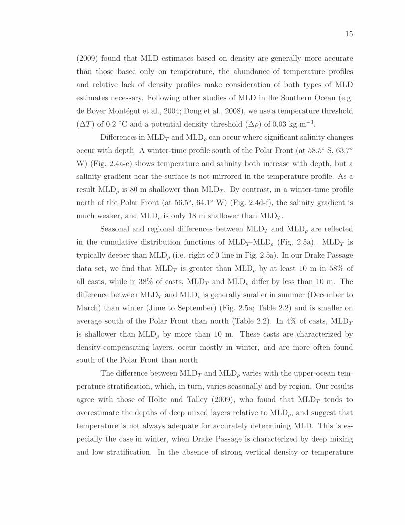
Differences in MLDT and MLDρ can occur where significant salinity changes

occur with depth. A winter-time profile south of the Polar Front (at 58.5◦ S, 63.7◦

W) (Fig. 2.4a-c) shows temperature and salinity both increase with depth, but a

salinity gradient near the surface is not mirrored in the temperature profile. As a

result MLDρ is 80 m shallower than MLDT . By contrast, in a winter-time profile

north of the Polar Front (at 56.5◦, 64.1◦ W) (Fig. 2.4d-f), the salinity gradient is

much weaker, and MLDρ is only 18 m shallower than MLDT .

Seasonal and regional differences between MLDT and MLDρ are reflected

in the cumulative distribution functions of MLDT -MLDρ (Fig. 2.5a). MLDT is

typically deeper than MLDρ (i.e. right of 0-line in Fig. 2.5a). In our Drake Passage

data set, we find that MLDT is greater than MLDρ by at least 10 m in 58% of

all casts, while in 38% of casts, MLDT and MLDρ differ by less than 10 m. The

difference between MLDT and MLDρ is generally smaller in summer (December to

March) than winter (June to September) (Fig. 2.5a; Table 2.2) and is smaller on

average south of the Polar Front than north (Table 2.2). In 4% of casts, MLDT

is shallower than MLDρ by more than 10 m. These casts are characterized by

density-compensating layers, occur mostly in winter, and are more often found

south of the Polar Front than north.

The difference between MLDT and MLDρ varies with the upper-ocean tem-

perature stratification, which, in turn, varies seasonally and by region. Our results

agree with those of Holte and Talley (2009), who found that MLDT tends to

overestimate the depths of deep mixed layers relative to MLDρ, and suggest that

temperature is not always adequate for accurately determining MLD. This is es-

pecially the case in winter, when Drake Passage is characterized by deep mixing

and low stratification. In the absence of strong vertical density or temperature

16

gradients, it can be difficult to unambiguously determine the true depth of mixing

using MLD. To test the robustness of MLD estimates to the choice of threshold,

we perturbed ∆T by ±0.02 ◦C and ∆ρ by ±0.003 kg m−3, a ±10% change to the

threshold criteria used to compute MLDT and MLDρ, respectively. This proce-

dure is equivalent to perturbing the near-surface temperature or density by the

same amount, making this test also a measure of how much MLD might change in

response to a small surface heat or buoyancy exchange.

An example of the 10% perturbation in threshold is shown for a typical

winter profile from an XCTD cast north of the Polar Front (at 56.5◦ S, 64.1◦ W)

(Fig. 2.4d-f). MLDT has been computed using the original threshold criteria of

∆T = 0.20 ◦C (dashed line in Fig. 2.4d), and the 10% pertubations ∆T = 0.18 ◦C

(top dotted line in Fig. 2.4d) and ∆T = 0.22 ◦C (lower dotted line in Fig. 2.4d).

Decreasing the temperature threshold ∆T reduces MLDT from 242 m to 240 m,

while increasing ∆T deepens MLDT to 258 m (Fig. 2.4d). MLDρ is much more

sensitive to the change in ∆ρ threshold; reducing ∆ρ from 0.030 to 0.027 kg m−3

decreased MLDρ from 220 m to 120 m (Fig. 2.4f), while increasing ∆ρ increased

MLDρ to 230 m. By contrast, for the cast collected south of the Polar Front (at

58.5◦ S, 63.7◦ W) a 10% perturbation to ∆T and ∆ρ changed MLDT and MLDρ

by less than 2 m (Fig. 2.4a-c).

The average MLDT change in response to a threshold perturbation is larger

north of the Polar Front than south and is larger in winter than summer (Table 2.2).

A cumulative distribution function of changes in MLDT shows that perturbing the

threshold results in a small (5 m or less) change in MLDT ∼85% of the time, except

during winter (June-September) north of the Polar Front (Fig. 2.5b). The reduced

sensitivity south of the Polar Front may be a result of the stronger permanent

thermocline that provides a lower bound on MLD and results in smaller maximum

∆MLDT . Stronger near-surface temperature gradients in summer account for the

reduced summer-time sensitivity to threshold. On average, MLDρ and MLDT are

equally sensitive to threshold perturbations north of the Polar Front, and MLDρ

is a little more sensitive than MLDT south of the Polar Front (Table 2.2).

Because MLD is sensitive to small-amplitude noise, small differences be-

17

tween two adjacent profiles may result in large differences in MLD. Two tempera-

ture profiles from XBTs deployed only 10 km (∼1 hour) apart north of the Polar

Front (at 57.3◦ S and 57.4◦ S, 64.0◦ W on 19 September 2009) have MLDT of 263 m

(Fig. 2.6a) and 118 m (Fig. 2.6b). While these profiles share many features, such

as alternating warm and cold layers, a slight warming at 120 m is observed in the

southernmost profile (Fig. 2.6b), resulting in MLDs that differ by >100 m.

To quantify the cast-to-cast variability of MLD as observed in Figure 2.6,

we computed the root-mean-square (RMS) change in MLDT from one cast to the

next. We selected 5010 pairs of casts that occurred less than one hour apart

(typically <10 km spacing). The cast-to-cast difference in MLDT (± one standard

error) is much greater in winter (54±3 m) than summer (20±1 m) and is greater

north (40±1 m) than south (24±1 m) of the Polar Front. This agrees with the

examples shown in Figures 2.3a and 2.6; south of the Polar Front, MLD variations

are small, whereas large MLD changes over short spatial scales are common north

of the Polar Front.

2.4.2 Upper-ocean heat content

We expect heat content to show a more direct relationship to heat flux

forcing than MLD and to be less affected by cross-frontal differences in temperature

stratification than MLD. Potentially, this makes heat content a more consistent,

more robust, and less noisy measure of upper-ocean variability. In this section,

we examine whether upper-ocean heat content estimated from the Drake Passage

data set fulfills this expectation.

We define Hz0, the upper-ocean heat content integrated from the surface to

a depth z0, to be

Hz0=

∫

0

−z0

ρ0 cp T (z) dz, (2.2)

where ρ0 = 1030 kg m−3 is a reference density, cp = 3895 J kg −1◦C−1 is the

specific heat capacity of seawater, T (z) is the depth-varying temperature, and z0

is an integration depth to be determined so as to capture the full effect of surface

forcing. To assess an appropriate integration depth, the heat content within 50 m

18

layers between 0 and 800 m depth was computed. Figure 2.7a shows the standard

deviation of the heat content over each depth interval for all casts, binned north and

south of the Polar Front. South of the Polar Front, the amplitude of variations

is small below about 200 m depth, while north of the Polar Front heat content

variability has more significant amplitude down to ∼600 m.

Figure 2.7b shows the correlation of heat content in the surface layer (0-

50 m) with heat content deeper in the water column. South of the Polar Front,

this correlation appears similar to the standard deviation (Fig. 2.7a); surface heat

content changes are significantly correlated with heat content changes in layers

above 200 m. North of the Polar Front, significant correlation with surface layer

heat content are found in layers above ∼350 m. Changes below this depth are

uncorrelated with heat content changes in the surface layer (Fig. 2.7b), but still

represent a significant fraction of the variability present north of the Polar Front

(Fig. 2.7a). The vertical coherence of this additional heat content variability below

350 m is shown by the correlation of heat content in the layer at 750-800 m, the

deepest layer for which we had reliable XBT profiles, with heat content in the

rest of the water column (Fig. 2.7b). Heat content changes at 750-800 m are

well-correlated (r > 0.8) with heat content changes in layers below ∼300 m depth

south of the Polar Front and below ∼200 m depth north of the Polar Front. This

level of vertical coherence is typical of the low-stratification environment of the

Southern Ocean and is often associated with advective processes (Sokolov and

Rintoul, 2009).

This study aims to test the adequacy of a 1-D heat budget in Drake Passage,

forced only by surface heat fluxes; other processes, such as advection, may degrade

the validity of this first-order heat balance. The choice of integration depth, z0 in

equation (2.2), reflects a trade-off between capturing as much of the surface-forced

signal as possible while avoiding variability unrelated to surface heat fluxes. Based

on Figure 2.7b, a choice of z0= 400 m is likely to reflect all of the heat content

signal that is significantly correlated with the surface layer; 400 m is deeper than

99% of the MLDT estimates. As noted above, vertically-coherent and presumably

advective processes below 200 m depth contribute significantly to heat content

19

variability north of the Polar Front. Selecting z0= 400 m rather than a deeper

integration depth reduces the weight of this variability relative to surface-forced

variability, but does not exclude variability resulting from other processes. For

z0= 400 m, 77% of the vertically-integrated temporal and spatial variance in heat

content is captured north of the Polar Front and 92% is captured south of the Polar

Front. The sensitivity of our results to this choice of z0 is discussed in section 2.5.

As noted in the introduction, a number of previous studies have examined

the heat budget within the mixed layer (e.g. Qiu and Kelly, 1993; Dong et al.,

2007). To directly compare the variability of heat content in equation (2.2) with

MLD, we also examine the heat content within the mixed layer. Mixed-layer heat

content, HML, is defined as

HML = ρ0 cp TML hML, (2.3)

where hML is the depth of the mixed layer (MLDT ), and TML is the mixed-layer

temperature. This quantity is not always directly computed in mixed-layer heat

budgets, which more often use MLD to relate heat fluxes to the rate of change of

the mixed-layer temperature, but it provides a good analog for Hz0because the

units are the same. Mixed-layer heat budgets often assume that the mixed layer is

isothermal, and equation (2.3) represents the mixed-layer heat content under this

assumption.

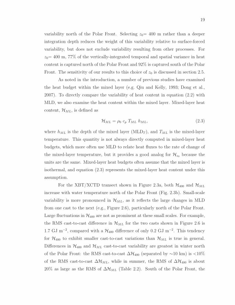
For the XBT/XCTD transect shown in Figure 2.3a, both H400 and HML

increase with water temperature north of the Polar Front (Fig. 2.3b). Small-scale

variability is more pronounced in HML, as it reflects the large changes in MLD

from one cast to the next (e.g., Figure 2.6), particularly north of the Polar Front.

Large fluctuations in H400 are not as prominent at these small scales. For example,

the RMS cast-to-cast difference in HML for the two casts shown in Figure 2.6 is

1.7 GJ m−2, compared with a H400 difference of only 0.2 GJ m−2. This tendency

for H400 to exhibit smaller cast-to-cast variations than HML is true in general.

Differences in H400 and HML cast-to-cast variability are greatest in winter north

of the Polar Front: the RMS cast-to-cast ∆H400 (separated by ∼10 km) is <10%

of the RMS cast-to-cast ∆HML, while in summer, the RMS of ∆H400 is about

20% as large as the RMS of ∆HML (Table 2.2). South of the Polar Front, the

20

differences in cast-to-cast RMS variability are not as extreme; in winter the RMS

of ∆H400 is about 20% as large as ∆HML, while in summer the RMS ∆H400 is

30% as large as RMS ∆HML (Table 2.2). Not only does H400 exhibit smaller

RMS cast-to-cast variability than HML, but it is also more consistent from season

to season. Cast-to-cast variability in HML is 3-4 times greater in winter than

in summer; for H400, RMS cast-to-cast variability in winter is less than twice as

great as in summer (Table 2.2). This demonstrates one way in which the use of

MLDT may present a distorted picture of seasonal variability that enhances the

apparent upper-ocean variability in winter relative to summer. Use of H400, with

its smaller season-to-season differences in RMS cast-to-cast variability, may reduce

this distortion.

2.5 Seasonal heating and cooling of the upper

ocean

As a first step towards understanding the seasonal variability of upper-ocean

heat content, we examined the annual pattern of heat fluxes and the expected

changes in heat content. As shown in Table 2.1, the amplitude of the seasonal

cycle in heat fluxes is approximately 130 W m−2, with a maximum around 25

December. If a heat flux forcing with this amplitude and phase is integrated in

time, it yields an annual cycle in heat content of ∼0.66 GJ m−2 that peaks on 25

March (green line, Fig. 2.8a,b). In this section, we test whether the mixed-layer

and upper-ocean heat budgets reflect this seasonal surface heat input.

For our heat budget, we use a simplified first-order relationship between

the heat content H and the surface forcing Qnet in which

∂H∂t

= Qnet. (2.4)

This relationship neglects the effects of advection and vertical entrainment on

upper-ocean heat content. Although these other factors may be important to

mixed-layer heat budgets (e.g., Qiu and Kelly, 1993; Dong et al., 2007), our main

focus here is to isolate the influence of air-sea heat exchange on the ocean to

21

examine the expected first-order terms in the Southern Ocean.

In our estimate of the seasonal cycle in upper-ocean heat content, we av-

eraged casts that were collected north of the Polar Front separately from those

south of the Polar Front for each of the 85 transects (averages denoted by H). The

date of each cruise average was assigned as the median date of the casts from each

transect. A least-squares fit to an annual cycle was made for the time series of

HML (Fig. 2.8a) and H400 (Fig. 2.8b). North of the Polar Front, a seasonal cycle in

HML accounts for 38% of the variance and has an amplitude of 0.77 GJ m−2 with

a maximum occurring July 4, in the middle of austral winter (Fig. 2.8a). South of

the Polar Front, a seasonal cycle in HML with amplitude 0.47 GJ m−2 peaks on

March 7 and explains 83% of the variance in heat content. For H400 north of the

Polar Front, an annual cycle with amplitude 0.51 GJ m−2 peaks on April 8 and

explains 24% of the variance (Fig. 2.8b). South of the Polar Front, the annual cycle

has an amplitude of 0.58 GJ m−2, peaks on March 19, and explains 63% of the

variance. There are a number of reasons why the seasonal cycle explains a larger

fraction of the variance in HML than in H400. South of the Polar Front, MLD is

generally much less than 400 m, so that HML reflects variability nearer the surface,

where the seasonal pattern of heating and cooling is stronger. North of the Polar

Front, a large seasonal change in MLD, from very shallow in summer to very deep

in winter, contributes to the stronger seasonality in HML. In terms of phase, the

deep winter MLDs result in a mid-winter (August, Fig. 2.8a) maximum in HML

that occurs about 4 months after the date at which the cumulative heat input has

reached its maximum (March). Thus the phase of the seasonal surface heat input

agrees with the phase of H400 better than with the phase of HML (Fig. 2.8a).

We tested whether surface heat input and Hz0agreed similarly well for

other values of the integration depth z0. A least-squares fit to a sinusoidal annual

cycle was made for Hz0with z0 ranging from 50 to 800 m varying in 50 m incre-

ments. South of the Polar Front, the amplitude of the seasonal cycle changes only

slightly with depth below ∼100 m (Fig. 2.9a). As z0 increases, the date of the

maximum heat content south of the Polar Front is slightly delayed: at z0=50 m

the cycle peaks in early March, whereas at z0=800 m the peak occurs in late March

22

(Fig. 2.9b). South of the Polar Front, the heat fluxes explain 80% of the variance

at z0=100, decreasing to 27% at z0=800 m (Fig. 2.9c). North of the Polar Front,

the amplitude of the seasonal cycle in heat content changes more with increasing

z0, from 0.33 GJ m−2 at z0=100 m to 0.62 GJ m−2 at z0=750 m (Fig. 2.9a). The

peak heat content at z0=800 m occurs in late April, almost 8 weeks later than for

z0=100 m in late February (Fig. 2.9b). Heat fluxes explain 55% of the variance in

Hz0at z0=100 m, while less than 25% of the variance is explained for z0 >400 m

(Fig. 2.9c). At all depths, the amplitude of the annual cycle in heat content was

smaller than the 0.66 GJ m−2 annual cycle in heat input from surface fluxes. Tren-

berth and Fasullo (2010) note that reanalysis heat fluxes over the Southern Ocean

have a seasonally-varying bias that is greater in summer than winter. Removing

such a bias would reduce the amplitude of the annual cycle in heat flux input and

may lead to better agreement between the annual cycles in heat content and heat

input by surface fluxes.

These results are consistent with the patterns of temperature variance

(Fig. 2.7a) that show temperature variations to have higher amplitudes north of

the Polar Front than south, illustrating the differences in vertical heat transfer in

the two regions. South of the Polar Front, most heat content fluctuations occur

above 200 m (Fig. 2.7a); integrating deeper than 200 m adds very little new infor-

mation and so changes the seasonal cycle in heat content only slightly. North of

the Polar Front, however, a clear depth limit to heat content fluctuations is less

evident. Heat concentrates in the upper 100 m during the spring restratification,

but this heat is gradually mixed downward. The downward mixing of heat away

from the surface results in heating at depth that is delayed relative to the surface

(Fig. 2.9b). The maximum temperatures at 650-700 m north of the Polar Front,

for example, occur in late May (not shown); however, because we have integrated

over the whole water column above this depth, the average date of the maximum

in H700 north of the Polar Front occurs in April. Wintertime cooling at the surface

results in a nearly isothermal, cool, water column in the upper 800 m north of the

Polar Front around September, following which warming and restratification begin

anew. The combination of the abrupt cooling in September and the delay in heat

23

transfer from the surface to depth is part of the reason the sinusoidal fit to the in-

tegrated heat fluxes in Figure 2.8 explains less variance as z0 increases (Fig. 2.9c).

The amplitude of the seasonal cycle in surface heating also decreases with depth.

This suggests that the 1-D balance between heat fluxes and heat content degrades

as z0 increases, and the relative importance of other processes, such as horizontal

heat advection, may come into play. Finally, these results may also have implica-

tions for the choice of the integration depth z0 such that Hz0reflects the surface

forcing. South of the Polar Front, a choice of z0 >200 m appears to provide a

sufficient constraint. However, north of the Polar Front the relative importance

of surface heating to other processes in determining Hz0varies more greatly with

depth and suggests greater sensitivity in this region to the choice of z0.

The delay of heating with depth in the phase of the seasonal cycle can be

used to estimate an effective mixing rate in the upper ocean. In more vigorous

mixing regions, surface heating is transported downward quicker, and so less phase

change with depth is observed. Conversely, where mixing is less active, surface

heating takes longer to propagate downward, resulting in a longer delay of heating

with depth. To relate phase to mixing rate, we modeled mixing as an effective

diffusivity and numerically solved the heat equation for a system forced at the

surface by a sinusoidal annual cycle for a range of diffusivities, κeff . A relationship

was derived between κeff and the vertical gradient in phase of the resulting Hz0.

Our results indicate an annual average of κeff ≈ 10−3 m2s−1 over the upper 200

m of the water column in Drake Passage. While effective diffusivity may be an

incomplete representation of a broad array of upper-ocean mixing processes that

are not strictly diffusive (e.g. entrainment), our value compares favorably to other

measures of vertical diffusivities in this region (e.g., O(10−3 m2s−1) Thompson

et al., 2007).

2.6 Summary

In this study, we have used XBT/XCTD profiles and reanalysis heat flux

products to examine air-sea heat exchange in Drake Passage on a seasonal timescale.

24

We compared mixed-layer depth and heat content as two methods for measuring

the response of the upper-ocean to surface heat forcing. Results of this study show

that upper-ocean heat content is a robust indicator of upper-ocean variability due

to surface heat flux forcing in Drake Passage.

Regional differences and temporal variability in Drake Passage stratification

make it difficult to define MLD such that it is a true measure of the vertical extent

of air-sea forcing. Estimates of MLDT and MLDρ can disagree, suggesting that

temperature alone is inadequate to unambiguously determine MLD. Further, as

a result of low winter-time stratification, MLD estimates are not always robust;

low-amplitude forcing or slight changes to the criteria used to define MLD can lead

to large changes in MLD estimates. Perhaps as a consequence of the sensitivity of

MLD calculations to small differences in temperature profiles, MLDT also shows

considerable variability at small horizontal scales.

In contrast to MLD, upper-ocean heat content is a robust measure of upper-

ocean variability. Average cast-to-cast differences in H400 were 3 to 10 times smaller

than in HML; the cast-to-cast variability in H400 also changed less with season

and less between the zones north and south of the Polar Front than cast-to-cast

variability in HML. This suggests that H400 is a consistent measure of upper-ocean

variability north and south of the Polar Front and in both winter and summer.

A first-order heat balance between the seasonal cycles of anomalous heat

fluxes (minus the annual mean) and upper-ocean heat content explains a large

fraction (∼63%) of the variance of upper-ocean heat content to 400 m depth south

of the Polar Front and to a lesser extent (∼24%) north of the Polar Front. In

contrast, an annual cycle that used heat content over the mixed layer did not match

the surface-flux driven annual cycle as well in phase or in amplitude. However,

the phase and amplitude of the seasonal cycle in Hz0are somewhat sensitive to

the choice of integration depth, z0, particularly north of the Polar Front, where

the amplitude increases and the date of the maximum heat content is delayed as

integration depth increases. This is a result of heat mixing more deeply north of

the Polar Front than south.

Although we found reasonable agreement between seasonal cycles in upper-

25

ocean heat content and heat fluxes, the simple 1-D heat budget employed in this

study may not be a complete picture of the processes governing upper-ocean vari-

ability. Horizontal advection, whether zonal advection by the mean ACC flow

or meridional Ekman transport, is likely to be an important component of a full

upper-ocean heat budget. Particularly north of the Polar Front, advection of ed-

dies through Drake Passage may represent a large but transient departure from the

seasonal cycles of upper-ocean heat content we have calculated here. These pro-

cesses will be important to consider in constructing a more complete understanding

of the upper-ocean response to air-sea fluxes.

We have shown that upper-ocean heat content can be a useful measure of

the effects of air-sea heat flux forcing and may be more suitable for this purpose

than MLD. One of the attractions of using MLD in studies of the Southern Ocean

is the ability to couple remote-sensing observations of SST to an upper-ocean heat

budget. As in situ data in the Southern Ocean become more widely available, the

need for this proxy measurement of MLD that remotely-sensed SST provides may

be reduced. With the advent of Argo profiling floats, for example, there are now

a few thousand profiles collected each year in the Southern Ocean, offering the

prospect to observe the impact of upper-ocean heating and cooling directly.

26

Table 2.1: The annual mean net heat fluxes computed from NCEP, J-OFURO,and OAFlux heat flux products, averaged over gridpoints north (56-59◦ S) andsouth (59-62◦ S) of the climatological position of the Polar Front in the longituderange 60-64◦ W. A least-squares fit to a sinusoid with period 365.25 days gives theamplitude and phase of the annual cycle. One-sigma uncertainties were computedby multiplying the error estimates from the least-squares fitting procedure by thestandard deviation of the heat flux values. A Monte-Carlo method with N=105

was used to calculate the uncertainty on the date of maximum amplitude.

Heat FluxProduct

Region Annual MeanQnet (W m−2)

Amplitude ofcycle (W m−2)

Date of max.amplitude

NCEP North of PF 29.5±1.6 130±3.2 25 Dec. ±1day

South of PF 31.7±1.6 131±3.2 24 Dec. ±1day

J-OFURO North of PF 22.1±1.8 131±3.6 27 Dec. ±1day


OAFlux North of PF 39.4±1.7 137±3.4 25 Dec. ±1day


27

Table 2.2: Characteristics of MLD and heat content are described by region (north or south of the Polar Front) andseason (winter or summer). The average difference in MLD defined using temperature and density criteria (MLDT -MLDρ)was computed from XCTD casts. ∆ MLDT and ∆ MLDρ are the average changes in calculated MLD in response to a10% change in the thresholds used to calculate MLD with temperature (MLDT ) and density (MLDρ), respectively. Theuncertainties represent one standard error. Cast-to-cast ∆HML and ∆H400 are the RMS differences in mixed-layer heatcontent and heat content over 400 m depth respectively, over pairs of casts collected less than 1 hour (about 10 km) apart.N is the number of cast-pairs used to compute ∆HML and ∆H400.

Region Season MLDT -MLDρ ∆ MLDT ∆ MLDρ RMS cast-to-cast ∆HML

(GJ m−2)(N)

RMS cast-to-cast ∆H400

(GJ m−2)(N)North of PF Summer 13±2 m 2.4±0.6 m 3.0±1.1 m 0.56 (609) 0.12 (609)

Winter 48±7 m 7.1±1.5 m 8.2±2.2 m 1.99 (429) 0.16 (429)South of PF Summer 6±2 m 1.8±0.4 m 2.4±0.6 m 0.36 (643) 0.12 (643)

Winter 34±5 m 4.0±0.8 m 5.2±1.3 m 0.95 (560) 0.20 (560)

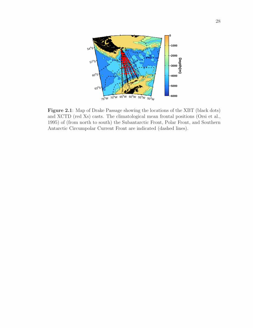
28

75oW 70oW 65oW 60oW 55oW 50oW

63oS

60oS

57oS

54oS

Depth(m

)

−6000

−5000

−4000

−3000

−2000

−1000

0

Figure 2.1: Map of Drake Passage showing the locations of the XBT (black dots)and XCTD (red Xs) casts. The climatological mean frontal positions (Orsi et al.,1995) of (from north to south) the Subantarctic Front, Polar Front, and SouthernAntarctic Circumpolar Current Front are indicated (dashed lines).

29

F M A M J J A S O N D

−100

−50

0

50

100

150

200

Qne

t (W

m−2

)

Figure 2.2: Monthly heat flux climatologies for NCEP (red), J-OFURO (blue),and OAFlux (black) over regions north (solid line) and south (dashed line) of theclimatological position of the Polar Front. Vertical lines indicate the two-sigmastandard error of a 30-day average.

30

Dep

th (

m)

−62 −61 −60 −59 −58 −57 −56 −55−600

−400

−200

0

Temperature ( o C)

−1 0 1 2 3 4 5 6

−62 −61 −60 −59 −58 −57 −56 −55−2

0

5

10

Hea

t con

tent

(G

J m

−2)

Latitude

a)

b)

Figure 2.3: (a) A section of temperature (◦C) from XBT casts during a DrakePassage transect 18-23 September 2009. The position of the Polar Front is indi-cated by the dashed magenta line. Mixed-layer depth (MLD) is indicated by theblack line. The latitude of example casts in Figures 2.4 and 2.5 are also indicated(triangles). (b) Mixed-layer heat content (solid black) and heat content integratedto 400 m (dashed line) for XBT casts from the transect in (a).

31

a) b) c)

d) e) f)

0 1 2−400

−300

−200

−100

0

Dep

th (

m)

34 34.5 27.2 27.3 27.4

3.6 3.8 4−400

−300

−200

−100

0

Dep

th (

m)

T (oC)34.05 34.1 34.15

S (psu) 27.05 27.1

σ (kg m −3)

Figure 2.4: Profiles from XCTD casts collected during the transect shown inFigure 2.3 on 20 September 2009 (a,b,c) near 58.5◦ S, 63.7◦ W and on 19 September2009 (d,e,f) near 56.5◦ S, 64.1◦ W. Profiles show temperature (◦C, a, d), salinity(psu, b, e), and potential density (kg m−3, c, f). MLDT is shown by the dashedline (a,b,d,e) and MLDρ is shown by the dash-dot lines (b,c,e,f). Dotted linesshow differences in MLDT (a,d) and MLDρ (c,f) after ∆T and ∆ρ are changed by±10%, respectively. In panels (a) and (c), these lines lie very close to the dashedline indicating MLDT . Note also that the x-axis scale is different for the upperand lower panels.

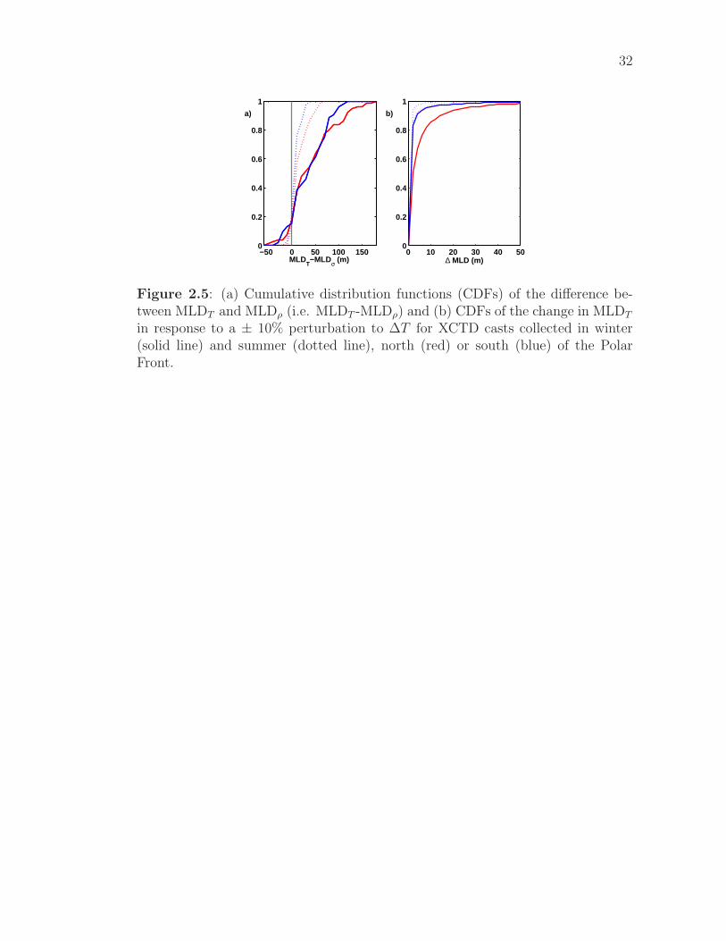
32

a) b)

−50 0 50 100 1500

0.2

0.4

0.6

0.8

1

MLDT−MLDσ (m) 0 10 20 30 40 50

0

0.2

0.4

0.6

0.8

1

∆ MLD (m)

Figure 2.5: (a) Cumulative distribution functions (CDFs) of the difference be-tween MLDT and MLDρ (i.e. MLDT -MLDρ) and (b) CDFs of the change in MLDT

in response to a ± 10% perturbation to ∆T for XCTD casts collected in winter(solid line) and summer (dotted line), north (red) or south (blue) of the PolarFront.

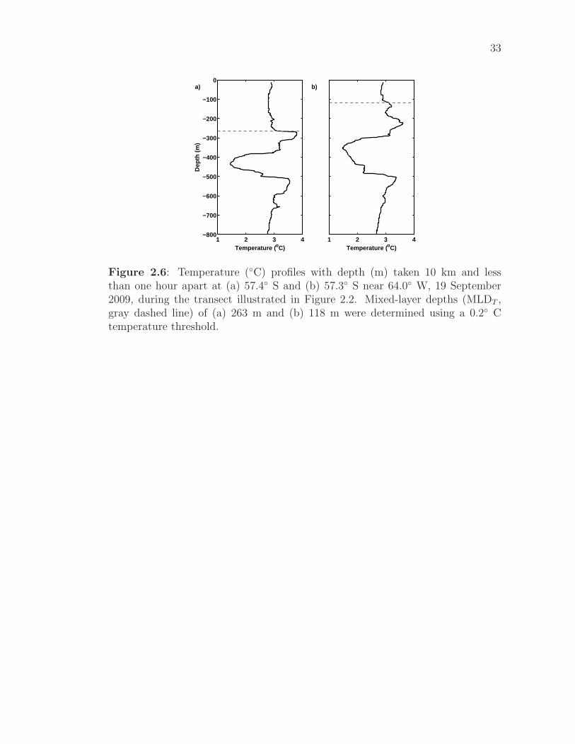
33

1 2 3 4−800

−700

−600

−500

−400

−300

−200

−100

0

Temperature ( oC)

Dep

th (

m)

1 2 3 4Temperature ( oC)

a) b)

Figure 2.6: Temperature (◦C) profiles with depth (m) taken 10 km and lessthan one hour apart at (a) 57.4◦ S and (b) 57.3◦ S near 64.0◦ W, 19 September2009, during the transect illustrated in Figure 2.2. Mixed-layer depths (MLDT ,gray dashed line) of (a) 263 m and (b) 118 m were determined using a 0.2◦ Ctemperature threshold.

34

0 0.1 0.2 0.3−800

−700

−600

−500

−400

−300

−200

−100

0

Dep

th (

m)

Std. Dev. (GJ m−2)0 0.5 1

Correlation

a) b)

Figure 2.7: (a) Standard deviation of heat content in 50-m layers north (solid)and south (dashed) of the Polar Front. (b) The correlation of heat content in theshallowest layer (0-50 m, black) and in the deepest layer (750-800 m, blue) withheat content in other layers north (solid) and south (dashed) of the Polar Front.The gray bar indicates correlations that are not significant and the red dotted linedelineates 400 m depth.

35

J F M A M J J A S O N D−2

0

2

4

HM

L (

GJ

m−2

)

J F M A M J J A S O N D0

2

4

6

8

10

H40

0 (G

J m

−2)

a)

b)

Figure 2.8: (a) HML, mean heat content over the mixed layer and (b) H400, heatcontent in the upper 400 m of the water column for casts north (red) and south(blue) of the Polar Front for 85 XBT transects are plotted against the median year-day of the cruise. Error bars (gray) represent the standard error of the mean. Asinusoidal annual cycle (dashed lines) is least-squares fit to each timeseries. Surfaceheat fluxes drive an annual cycle in heat content (green line, offset by 4 GJ m−2)made by integrating daily net heat flux anomalies (annual mean removed) fromNCEP.

36

0 0.5 1−800

−700

−600

−500

−400

−300

−200

−100

0

Dep

th (

m)

Amp. (GJ m −2)Mar Apr May

Date 0 50 100

% Var.

a) b) c)

Figure 2.9: (a) Amplitude and (b) phase of a sinusoidal annual cycle fit to Hz0

north (solid) and south (dashed) of the Polar Front for values of z0 ranging from50 to 800 m in 50 m increments. (c) The fraction of the variance in Hz0

explainedby an annual cycle in heat fluxes. The red dotted line indicates 400 m depth.

37

2.7 Acknowledgments

Data collection and analysis for this project was funded by NSF grants

to STG (ARRA OCE08050350) and JS (ANT0943818) and a NASA grant to

STG (NNX08AI82G). GRS would like to acknowledge a NASA Earth and Space

Science Fellowship and the ARCS Foundation for their support. STG acknowledges

sabbatical support from the French Centre National de la Recherche Scientifique.

Chapter II, in full, is a reprint with no modifications to content of the article

as it appears in Journal of Geophysical Research-Oceans, 2012, G.R. Stephenson

Jr., S.T. Gille, and J. Sprintall, reproduced with permission of American Geo-

physical Union. The dissertation author was the primary researcher and author of

this manuscript. Janet Sprintall provided the XBT/XCTD data and directed and

supervised the research along with Sarah Gille.

Chapter 3

Interannual variability of

upper-ocean heat content in

Drake Passage

38

39

3.1 Abstract

A 16-year record of expendable bathythermograph (XBT) transects across

Drake Passage is used to examine interannual variability in upper ocean heat con-

tent. The response of upper ocean heat content to anomalous heat fluxes, winds,

and two large-scale climate indices is examined. Results suggest that interannual

variations in surface heat fluxes explain ∼5-10% of the variability in upper-ocean

heat content. Anomalous surface heat fluxes are linked to meridional wind anoma-

lies upstream of Drake Passage, which are, in turn, linked to forcing by El Nino

/ Southern Oscillation (ENSO) and the Southern Annular Mode (SAM). ENSO

and SAM are correlated with upper ocean heat content at near-zero lags, although

relationships at longer time scales are also evident. Furthermore, differences in

response time scales to ENSO and the SAM are evident for heat content south

of the Polar Front versus north of the Polar Front. Interannual variability in up-

per ocean heat content due to mesoscale eddies and meanders is explored using

a tracked eddy database. An empirical relationship is constructed relating upper

ocean heat content anomalies to eddy length scales and amplitudes. Eddies and

meanders are estimated to account for more than one third of the interannual

variability in upper-ocean heat content in Drake Passage.

3.2 Introduction

In recent decades, the Southern Ocean has undergone significant warming

(e.g., Gille, 2008). Although heat uptake by the Southern Ocean may retard pro-

jected increases in global atmospheric temperatures over the next century (Boe

et al., 2009), an increase in sea water temperatures near the Antarctic continent

will also contribute to increased ice sheet melting and accelerated sea level rise (Ja-

cobs et al., 2011). More frequent positive El Nino / Southern Oscillation (ENSO)

events in recent decades (Kwok and Comiso, 2002) and a positive shift in the in-

dex of the Southern Annular Mode (SAM) (Thompson and Wallace, 2000) have

fuelled inquiries into the mechanisms that link large-scale atmospheric forcing to

Southern Ocean warming (e.g., Turner, 2004; Meredith et al., 2008; Ciasto and

40

England, 2011).

The mechanisms by which ENSO and the SAM affect the upper-ocean are

complex and inter-related. The major mode of atmospheric variability in the

Southern Ocean is the SAM, which manifests itself as a strengthening of the merid-

ional pressure gradient around Antarctica (Thompson and Wallace, 2000). With

this increase in the sea level pressure gradient comes an intensification and pole-

ward shift of the circumpolar winds (Hall and Visbeck, 2002). ENSO-derived

changes in sea surface temperature (SST) anomalies in the tropical Pacific lead

to atmospheric Rossby wave trains that propagate poleward as alternating cy-

clonic and anticyclonic (atmospheric) eddies (Turner, 2004; Meredith et al., 2008).

These atmospheric waves affect zonal and meridional surface winds and cloud

cover, and thereby influence surface heat fluxes over the Antarctic Circumpolar

Current (ACC); this results in cold SST anomalies near Drake Passage and a

warm SST anomaly ∼5000 km upstream (Meredith et al., 2008). Advection of the

upstream anomalies leads to a positive SST anomaly in Drake Passage ∼2 years

later (Meredith et al., 2008). Coupled anomalies in cloud cover, wind, SST, and

sea ice concentration have been associated with the Antarctic Circumpolar Wave

(ACW), an eastward propagating mode 2 wave in the ACC seen in data from

1985-1994 (White and Peterson, 1996), and the Antarctic Dipole (ADP), a mode

of heightened contrast between the southeast Pacific and the southwest Atlantic

(Yuan and Martinson, 2000). It has been suggested that the ACW and ADP, when

they occur, may be partly driven by ENSO variability (Yuan and Martinson, 2000;

Peterson and White, 1998).

To some extent, ENSO and SAM also covary; ENSO explains ∼25% of

the variance of SAM in austral summer (L’Heureux and Thompson, 2006). The

response of the ocean to forcing by ENSO and SAM occurs at many timescales and

varies geographically. The general response to a positive SAM is a poleward shift

in the position of the fronts of the ACC as a result of the corresponding poleward

shift in the wind (e.g., Hall and Visbeck, 2002; Sallee et al., 2008). In the southeast

Pacific, however, increased Ekman pumping and northward transport of cold, fresh

water associated with the shift in circumpolar winds leads to a northward shift

41

in the location of the fronts of the ACC (Sen Gupta and England, 2006; Sallee

et al., 2008). In the same region, a positive ENSO index (El Nino conditions)

is associated with a poleward displacement of ACC fronts (Sallee et al., 2008).

Observations suggest that eddy kinetic energy (EKE) in the ACC responds to the

SAM and ENSO after a 1-3 year lag, albeit with a response that varies regionally

(Morrow et al., 2010). Positive SAM index leads to an increase in EKE in the

south Pacific after a 2-3 year lag (Morrow et al., 2010). Negative ENSO (La

Nina conditions) tend to increase EKE after a 1-2 year lag, while positive ENSO

decreases EKE after a 1-2 year lag (Morrow et al., 2010). The increased EKE may

result in increased meridional heat transport (e.g., Boning et al., 2008), potentially

of sufficient magnitude to account for the observed warming of the Southern Ocean

(Hogg et al., 2008). Such changes in the Southern Ocean meridional transport

have global effects, as forcing by the SAM may alter the strength of the meridional

overturning circulation on decadal timescales (e.g., Sijp and England, 2009; Marini

et al., 2011).

Drake Passage is a good location for studies of the effects of ENSO and the

SAM on the upper ocean, as heat content anomalies in the south Pacific must pass

through Drake Passage to reach the other ocean basins. In this study, we identify

the effects of ENSO and SAM on upper ocean heat content and evaluate the impor-

tance of these two modes of atmospheric forcing to the overall variability in heat

content of the ocean. Other processes are likely to be equally important. Previous

work has shown that in Drake Passage seasonal surface heat fluxes explain ∼24%

of the variance in upper-ocean heat content north of the Polar Front and ∼63%

of the variance in upper-ocean heat content south of the Polar Front (Stephen-

son et al., 2012). A good one-dimensional balance between heat fluxes and upper

ocean heat content exists on seasonal time scales (Stephenson et al., 2012). It is

unclear how well this balance will hold on interannual time scales, since meanders

of the ACC fronts and advection of eddies are likely to be significant contributors

to upper ocean variability in the Drake Passage region (Sprintall, 2003; Lenn et al.,

2007; Sprintall, 2008). The goal of this study is to assess the contributions of each

of these sources of interannual variability to the upper-ocean in Drake Passage.

42

Section 3.3 describes the data sets used in this work. In Section 3.4, we review

the characteristics of upper-ocean temperature variability in Drake Passage and

describe upper-ocean heat content anomalies. In Section 3.5, the temporal and

spatial scales relating atmospheric variability and climate forcing to heat content

anomalies are determined using linear correlations at various time lags. Section 3.6

addresses upper-ocean variability due to eddies and frontal meanders identified in

the Chelton et al. (2011b) tracked eddy database. In Section 3.7, we estimate the

relative contributions of heat fluxes, meanders and eddies, and forcing by ENSO

and the SAM to upper ocean heat content. Section 3.8 summarizes our findings

and presents our conclusions.

3.3 Data

3.3.1 Temperature transects

The heat content of the upper several hundred meters of the water column

is examined using temperature transects from the Scripps High Resolution expend-

able bathythermograph / expendable conductivity, temperature, depth (XBT/XCTD)

program. Since September 1996, operations on the ASRV L. M. Gould have in-

cluded underway deployment of XBTs on 6-7 Drake Passage crossings each year

(Fig. 3.1). The use of expendable devices makes routine hydrographic measure-

ments possible even in adverse weather conditions without unduly impacting nor-

mal ship operations, such that XBT transects across Drake Passage have been

performed in all seasons. Each transect takes 2-3 days, during which ∼70 XBTs

are deployed at 10-15 km spacing, or 6-10 km spacing across the Subantarctic and

Polar Fronts. The Polar Front is defined here as the northward extent of the 2 ◦C

isotherm at 200 m depth (Orsi et al., 1995). XBT probes typically return temper-

ature profiles to their rated depth of 850 m. The fall-rate correction of Hanawa

et al. (1995) has been applied to each profile, and profiles are averaged to 2 m

vertical resolution. Between September 1996 and August 2011, 99 transects were

collected. Of these, three transects terminated north of 60oS (September 1997,

February 1998, and July 1999) and three transects deviated significantly from the

43

typical crossings shown in Figure 3.1 (September 1999, June 2000, and January

2009). Data from these cruises have been excluded from our analysis. For each

of the remaining 93 transects, temperature fields from the XBTs have been objec-

tively mapped onto a regular grid with 10 m vertical resolution and 0.1o latitude

horizontal spacing (Sprintall, 2003).

3.3.2 Eddy database

Sea surface height fields can be used to identify mesoscale eddies. The

simplest methods involve identifying constant contours of sea surface height (e.g.,

Sprintall, 2003; Fang and Morrow, 2003) or calculating Okubo-Weiss parameters

(e.g., Isern-Fontanet et al., 2003). In this study, we use the database of eddies

identified in weekly, gridded AVISO SSH fields by Chelton et al. (2011b). Their

algorithm uses a range of thresholds to search a map of SSH anomaly for eddies

with areas between 8 and 1000 pixels containing a local maximum or minimum,

with amplitude of at least 1 cm. This algorithm for eddy identification differs from

prior methods in that no thresholds (of SSH or other parameters) need be specified

since a wide range of possible values are searched and the SSH fields do not need

to be smoothed or differentiated. Eddy-like features are tracked from one weekly

SSH field to the next; only those features lasting at least 4 weeks are included in

the database.

The database includes information about eddies such as their center latitude

and longitude, effective length scale and amplitude. The boundary of an eddy is

identified as the location of the maximum current averaged along a contour. The

area of the bounded region is calculated and the “effective length scale” of the

eddy is reported as the radius of a circle whose area equals the bounded area.

Amplitude is given by difference between the sea surface height anomaly at the

center of the eddy and the sea surface height anomaly at the boundary (Chelton

et al., 2011b). Thus, cyclonic (cold-core) eddies have a negative amplitude, and

anti-cyclonic (warm-core) eddies have a positive amplitude. The eddies in the

Chelton et al. (2011b) database were identified using AVISO fields from October

1992 through January 2011, providing information about eddies in all but the

44

three most recent cruises we examined. To identify XBT transects that intersected

eddies, we interpolated eddy positions and properties (length scale and amplitude)

linearly in time to match the median date of the XBT transect. We determined

that an eddy was sampled if the distance from the eddy center to one or more

XBT casts was less than the eddy’s effective length scale.

3.3.3 Heat fluxes and wind fields

Stephenson et al. (2012) examined three heat flux products in Drake Passage–

NCEP-NCAR Reanalysis 1 heat fluxes (Kalnay et al., 1996), Objectively Analyzed

fluxes (Yu and Weller, 2007), and Japanese Ocean Fluxes with Use of Remote-

sensing Observations (Kubota et al., 2002)–and found them to be similar on sea-

sonal timescales. For this study, we employed NCEP-NCAR Reanalysis 1 heat

fluxes, a daily, gridded product with resolution ∼1.9◦ x 1.9◦ sampled over 1 Jan-

uary 1996 - 31 December 2011, as this heat flux product overlaps the entire time

span of the XBT transect time series. Heat fluxes in the vicinity of Drake Pas-

sage (270-305oE, 54-65oS) were smoothed with a 60-day running mean. Heat flux

anomalies were computed relative to a daily climatology of fluxes at each gridpoint.

Interannual variability in wind forcing was explored using wind fields from

the same NCEP-NCAR Reanalysis 1 fields (Kalnay et al., 1996). The 10 m zonal

and meridional components of the wind were smoothed with a 60-day Loess filter.

Wind anomalies were computed relative to a daily climatology at each gridpoint.

3.3.4 Climate indices

To examine the influence of major modes of climate variability, we used

lagged correlations of upper-ocean heat content with climate indices. We use a

monthly, multivariate ENSO index based on principal component analysis of six

observed variables in the tropical Pacific (Wolter and Timlin, 1998): sea-level

pressure, two components of surface wind, sea surface temperature, surface air

temperature, and cloud fraction. For the SAM index we use the monthly values

based on zonally-averaged sea level pressure differences between 40oS and 70oS

45

(Nan and Li, 2003).

3.4 Upper-ocean heat content

Drake Passage is a dynamically active region where transport of ∼140 Sv

(Cunningham et al., 2003; Firing et al., 2011) passes through a 700 km wide gap.

The strong flow is accompanied by strong temperature gradients at the ACC fronts

(Orsi et al., 1995; Sokolov and Rintoul, 2009). The Subantarctic Front, Polar Front,

and southern ACC Front, divide Drake Passage into regions with very different

temperature and density stratification (Orsi et al., 1995; Sprintall, 2003). South of

the Polar Front, cold Antarctic Surface Water (AASW) lies above a warmer, more

saline Circumpolar Deep Water (CDW) (Figure 3.2a,b). North of the Polar Front,

temperature stratification is much lower, with near-vertical isotherms possible to

depths >800 m (Figure 3.2a,b).

The upper ocean heat content is a useful measure for understanding upper-

ocean variability (e.g., Willis et al., 2004; Stephenson et al., 2012). In this study,

we define upper-ocean heat content over the upper 400 m of the water column of

a single profile, h400, as

h400 =

∫

0

−400

ρ0cpT (z)dz, (3.1)

where ρ0 = 1030 kg m−3 is the density of seawater, cp = 3985 J kg m−3 is the

heat capacity of seawater, and T (z) is the temperature at depth z. The choice of

400 m as an integration depth is motivated by the following considerations: first,

temperature variations are small below 400 m south of the Polar Front; second,

while more variability is present below 400 m north of the Polar Front, temperature

changes at 400 m were strongly correlated with changes down to 800 m, so most of

the variability in upper-ocean heat content can be understood by considering h400

(Stephenson et al., 2012).

Two winter transects illustrate interannual variability in h400 in the region.

In the first transect, sampled 10-12 June 2006 (Figure 3.2a), the Polar Front is

found at 58.3oS. In the second transect, sampled 28-30 June 2009 (Figure 3.2b), the

Polar Front is located ∼50 km farther south at 58.8oS. The minimum temperature

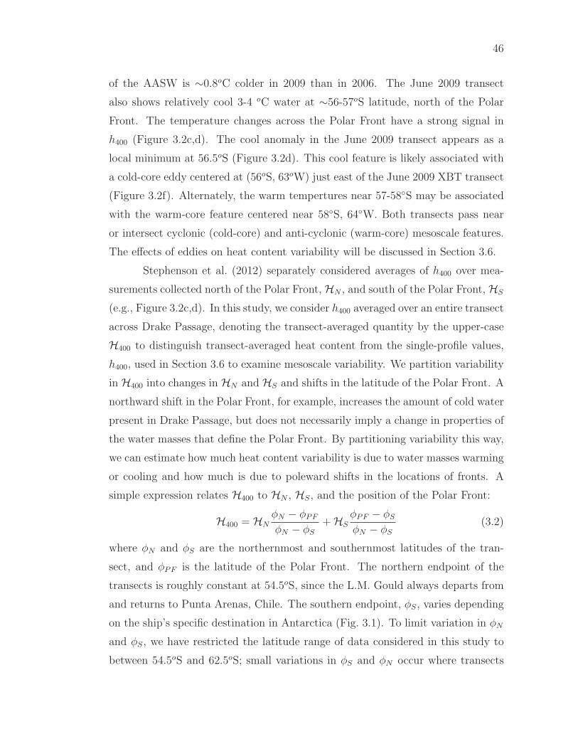
46

of the AASW is ∼0.8oC colder in 2009 than in 2006. The June 2009 transect

also shows relatively cool 3-4 oC water at ∼56-57oS latitude, north of the Polar

Front. The temperature changes across the Polar Front have a strong signal in

h400 (Figure 3.2c,d). The cool anomaly in the June 2009 transect appears as a

local minimum at 56.5oS (Figure 3.2d). This cool feature is likely associated with

a cold-core eddy centered at (56oS, 63oW) just east of the June 2009 XBT transect

(Figure 3.2f). Alternately, the warm tempertures near 57-58◦S may be associated

with the warm-core feature centered near 58◦S, 64◦W. Both transects pass near

or intersect cyclonic (cold-core) and anti-cyclonic (warm-core) mesoscale features.

The effects of eddies on heat content variability will be discussed in Section 3.6.

Stephenson et al. (2012) separately considered averages of h400 over mea-

surements collected north of the Polar Front, HN , and south of the Polar Front, HS

(e.g., Figure 3.2c,d). In this study, we consider h400 averaged over an entire transect

across Drake Passage, denoting the transect-averaged quantity by the upper-case

H400 to distinguish transect-averaged heat content from the single-profile values,

h400, used in Section 3.6 to examine mesoscale variability. We partition variability

in H400 into changes in HN and HS and shifts in the latitude of the Polar Front. A

northward shift in the Polar Front, for example, increases the amount of cold water

present in Drake Passage, but does not necessarily imply a change in properties of

the water masses that define the Polar Front. By partitioning variability this way,

we can estimate how much heat content variability is due to water masses warming

or cooling and how much is due to poleward shifts in the locations of fronts. A

simple expression relates H400 to HN , HS, and the position of the Polar Front:

H400 = HNφN − φPF

φN − φS

+ HSφPF − φS

φN − φS

(3.2)

where φN and φS are the northernmost and southernmost latitudes of the tran-

sect, and φPF is the latitude of the Polar Front. The northern endpoint of the

transects is roughly constant at 54.5oS, since the L.M. Gould always departs from

and returns to Punta Arenas, Chile. The southern endpoint, φS, varies depending

on the ship’s specific destination in Antarctica (Fig. 3.1). To limit variation in φN

and φS, we have restricted the latitude range of data considered in this study to

between 54.5oS and 62.5oS; small variations in φS and φN occur where transects

47

are terminated within this range. For the 93 Drake Passage transects, HN , HS,

and φPF (as in equation 3.2) each contribute roughly one third of the variability

in H400 (Table 3.1).

To define heat content anomalies associated with interannual variability, we

remove a seasonal cycle from the transect-averaged heat content (Figure 3.3). A

least-squares fit was made to annual and semi-annual harmonics; this fit explained

∼50% of the variability in H400. Similarly constructed fits explain ∼30% and

∼70% of the variability in HN and HS, respectively (Table 3.1). The residuals left

when seasonal cycles are removed are denoted H′400

(Fig. 3.3), H′N , and H′

S. We

note that H′S has a standard deviation (0.37 GJ m−2) half as large as that of H′

N

(0.68 GJ m−2). Movements of the Polar Front explain ∼34% of the interannual

variability in H′400

, whereas H′N explains ∼26% of the variance in H′

400and HS

explains only 9% of the variance in H′400

(Table 3.1). This implies that on interan-

nual timescales changes in water temperature south of the Polar Front contribute

less to the overall variability of upper ocean heat content in Drake Passage than

shifts in the Polar Front location and changes in heat content north of the Polar

Front.

3.5 Variability due to atmospheric forcing

Atmosphere-ocean interactions at the sea surface are a primary driver of

upper-ocean variability. On seasonal timescales, upper-ocean heat content appears

to be governed by surface heat flux forcing (Stephenson et al., 2012). Interannual

variability in surface heat fluxes is also expected to have a direct influence on upper-

ocean heat content. A number of studies have found a response of the upper ocean

to modes of large-scale atmospheric variability, in the form of frontal movements or

SST changes (e.g., Sallee et al., 2008; Meredith et al., 2008). ENSO and the SAM

have also been tied to changes in surface wind stress (Turner, 2004) and surface and

Ekman heat fluxes in the Southern Ocean (Ciasto and England, 2011). This section

examines contributions to interannual upper-ocean heat content variability arising

from changes in surface heat input, and links heat flux anomalies to meridional

48

wind anomalies upstream of Drake Passage. Finally, we examine the response

of H′400

to large-scale forcing using linear correlations with the ENSO and SAM

indices.

Heat fluxes represent a time rate of change of upper-ocean heat content.

The change in ocean heat content resulting from surface heat fluxes, ∆H, can be

expressed as a simple time integral

∆H =

∫ t2

t1

Q′net dt (3.3)

from time t1 to t2, where Q′net is the net surface heat flux anomaly defined in

Section 3.3.3. This is potentially a highly simplified expression. In a highly ad-

vective region, such as the ACC, heat anomalies due to local surface heat fluxes

are advected downstream, affecting heat content downstream at a time offset that

depends on the distance and speed of the advection. Furthermore, since ∆H has

no explicit depth scale and vertical mixing within the water column may distribute

heat flux input to depths deeper than 400 m, the relationship between Q′net and

H′400

may be weakened. Therefore, this calculation requires careful consideration of

the horizontal, vertical, and temporal scales over which a signal is likely to persist.

Nontheless, prior work suggests that more than 75% of the upper-ocean thermal

variability occurs above 400 m depth (Stephenson et al., 2012).

To determine where heat flux anomalies contribute most to heat content in

Drake Passage, we constructed a map of the correlation between H′400

and Q′net

at points in and upstream of Drake Passage over a range of time offsets. The

maximum correlation was found for Q′net at 60oS, 289oE at a time offset of 75 days

(i.e., heat flux anomalies 75 days prior to a transect, Q75d) (r =0.42, Fig. 3.5a). In

fact, lagged correlations of Q′net at this location with H′

400have significant positive

correlations spanning a range of time offsets from 55-80 days (Fig. 3.5b). At these

time offsets, significant positive correlations cover a large area upstream (from

∼58-64oS, 277-300oE) of Drake Passage (Fig. 3.5a). We thus conclude that this

correlation is not overly sensitive to the time offset or location. The regression

coefficient between heat fluxes at 60oS, 289oE and H′400

is 7.6±4.6×10−3 GJ W−1

(significant at p=0.99); this is equivalent to the heat accumulated by a constant

1 W m−2 heat flux over a time period of 88±53 days, or roughly 3±2 months.

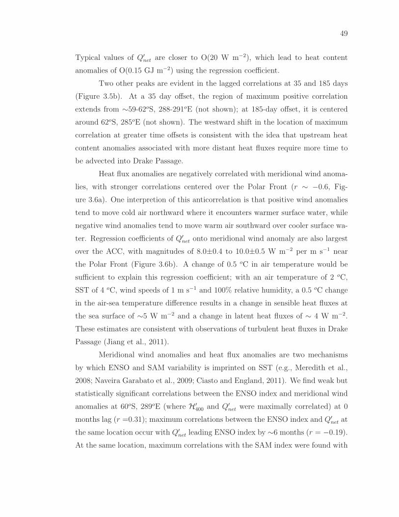
49

Typical values of Q′net are closer to O(20 W m−2), which lead to heat content

anomalies of O(0.15 GJ m−2) using the regression coefficient.

Two other peaks are evident in the lagged correlations at 35 and 185 days

(Figure 3.5b). At a 35 day offset, the region of maximum positive correlation

extends from ∼59-62oS, 288-291oE (not shown); at 185-day offset, it is centered

around 62oS, 285oE (not shown). The westward shift in the location of maximum

correlation at greater time offsets is consistent with the idea that upstream heat

content anomalies associated with more distant heat fluxes require more time to

be advected into Drake Passage.

Heat flux anomalies are negatively correlated with meridional wind anoma-

lies, with stronger correlations centered over the Polar Front (r ∼ −0.6, Fig-

ure 3.6a). One interpretion of this anticorrelation is that positive wind anomalies

tend to move cold air northward where it encounters warmer surface water, while

negative wind anomalies tend to move warm air southward over cooler surface wa-

ter. Regression coefficients of Q′net onto meridional wind anomaly are also largest

over the ACC, with magnitudes of 8.0±0.4 to 10.0±0.5 W m−2 per m s−1 near

the Polar Front (Figure 3.6b). A change of 0.5 oC in air temperature would be

sufficient to explain this regression coefficient; with an air temperature of 2 oC,

SST of 4 oC, wind speeds of 1 m s−1 and 100% relative humidity, a 0.5 oC change

in the air-sea temperature difference results in a change in sensible heat fluxes at

the sea surface of ∼5 W m−2 and a change in latent heat fluxes of ∼ 4 W m−2.

These estimates are consistent with observations of turbulent heat fluxes in Drake

Passage (Jiang et al., 2011).

Meridional wind anomalies and heat flux anomalies are two mechanisms

by which ENSO and SAM variability is imprinted on SST (e.g., Meredith et al.,

2008; Naveira Garabato et al., 2009; Ciasto and England, 2011). We find weak but

statistically significant correlations between the ENSO index and meridional wind

anomalies at 60oS, 289oE (where H′400

and Q′net were maximally correlated) at 0

months lag (r =0.31); maximum correlations between the ENSO index and Q′net at

the same location occur with Q′net leading ENSO index by ∼6 months (r = −0.19).

At the same location, maximum correlations with the SAM index were found with

50

Q′net leading the SAM by 2 months (r =0.17) and with meridional wind anomalies

leading the SAM by 1 month (r =0.20).

To observe the oceanic response to general forcing by ENSO and SAM, we

calculated lagged correlations of the ENSO and SAM indices with H′400

, φPF , H′N ,

and H′S (Figure 3.7) at time offsets from -6 months to +6 years. To accommodate

the irregular temporal sampling of the XBT transects, we linearly interpolated the

monthly ENSO and SAM indices so as to keep the time offset from the date of the

XBT transects constant for each correlation. Positive lags indicate that a transect

occurs after the climate index.

The strongest correlations with ENSO occur when H′400

leads the ENSO

index by 1-3 months (r =-0.45, Fig. 3.7a). At this time lag, El Nino is associated

with cooling of H′400

, a northward shift of the Polar Front, and cooling of H′S

(Fig. 3.7). Similarly, La Nina is associated with warming of H′400

, a southward

shift of the Polar Front, and warming of H′S (Fig. 3.7). This relationship may

be explained by anomalous heat flux input upstream of Drake Passage. Recall

that Q′net at 60oS, 289oE leads the ENSO index by 6 months; if the resulting heat

content anomalies require 2-3 months (∼75 days) to reach Drake Passage, we would

expect a signal in H′400

that leads the ENSO index by 3-4 months. The time scale

of this response also shows good agreement with results by Meredith et al. (2008);

they found a negative response of SST near South Georgia Island, ∼1500 km

east of Drake Passage, at a lag of 5 months, but estimated that SST anomalies

advected by the ACC would require 5-6 months to reach South Georgia Island

from the western Antarctic Peninsula. We also find significant correlations at time

lags of 4.5 years (54 months), when ENSO and H′400

are negatively correlated

(r =-0.27), ENSO and φPF are positively correlated (r =0.31) and ENSO and

H′N are negatively correlated (r =-0.24). Meredith et al. (2008) found a negative

correlation of South Georgia SST with ENSO at a lag of 60 months. So if the signal

from ENSO is advected to South Georgia from Drake Passage in 5-6 months, a

minimum in the correlation of Drake Passage heat content with ENSO would be

expected at 54 months lag, consistent with what we observe. At a time lag of

10-11 months, ENSO and H′400

are positively correlated (r =0.24, Fig. 3.7a), as

51

are ENSO and H′N (r =0.26, Fig. 3.7c). The mechanism responsible for the time

scale of this correlation is not clear. The atmospheric Rossby waves associated

with ENSO are thought to imprint an SST anomaly in the south Pacific, but

advection of this anomaly from the south Pacific to Drake Passage is expected

to take ∼2 years (Meredith et al., 2008). South of the Polar Front, upper ocean

heat content responds to ENSO on a different time scale. Correlations of H′S with

ENSO have a peak at a lag of ∼3 years (r =0.27), when correlations of ENSO with

H′400

, φPF and H′N are not significant. This response is slower than the expected

∼2 years (Trathan and Murphy, 2002; Meredith et al., 2008); positive correlations

between ENSO and H′S at a 3 year lag are consistent with a similar response of

Winter Water layer temperatures to ENSO at 3 year lag (Sprintall, 2008). The

response of H′S to forcing by ENSO may be mediated by interactions between the

upper ocean and sea-ice, as sea-ice extent near the western Antarctic Peninsula

is positively correlated with ENSO forcing at lags of 18-30 months (Yuan and

Martinson, 2000), comparable to the ∼3 year response of H′S.

The response of H′400

to forcing by the SAM occurs at two timescales

(Fig. 3.7). Near zero lag, positive correlations occur when H′400

leads the SAM

by 1 month (r =0.22) or lags the SAM by 3 months (r =0.22). The maximum cor-

relation of the SAM with H′N occurs when H′

N leads the SAM by 1-5 months, with

warm anomalies in H′N being associated with a positive SAM and cold anoma-

lies being associated with a negative SAM (r =0.27). These responses may be

driven by heat fluxes or meridional wind anomalies associated with the SAM. The

positive response of H′400

and H′N to the SAM on short timescales mirror similar

relationships between the SAM and SST (e.g., Kwok and Comiso, 2002; Liu et al.,

2004) and between the SAM and temperatures at depths of 0 to 400 m north of

the Polar Front (Sprintall, 2008). A second response to the SAM is seen at a lag

of ∼38 months, when correlations with H′400

and H′N are negative (r =-0.23 and

r =-0.24, respectively) and correlation with φPF is positive (r =0.20), correspond-

ing to a northward movement of the Polar Front in response to a positive SAM

index 38 months prior or a southward movement of the Polar Front in response

to a negative SAM index 38 months prior. At a lag of 2 years, Sprintall (2008)

52

found that the SAM was associated with cooler near-surface temperatures north

of the Polar Front. One expected response to the SAM is an increase in EKE

(Morrow et al., 2010) and meridional heat transport (Hogg et al., 2008). Nega-

tive correlations of H′400

and H′N with the SAM at this lag are consistent with

this possibility; increased EKE can lead to upwelling north of the Polar Front and

an increase in the northward transport of Winter Water / Antarctic Intermedi-

ate Water (Naveira Garabato et al., 2009). Both processes are compatible with

cooling north of the Polar Front. The response of heat content south of the Polar

Front occurs at shorter time lags; our results show peaks in the correlations of the

SAM with H′S at lags of 6 months (r =0.27) and 18-24 months (r =0.40). Warm

anomalies in H′S may result from increased upwelling of warm upper Circumpolar

Deep Water in response to increased zonal wind stress associated with the SAM.

Several studies have also emphasized the importance of interactions between atmo-

spheric forcing, sea-ice extent along the western Antarctic Peninsula, and resulting

changes to the upper ocean (e.g., Yuan and Martinson, 2000; Meredith et al., 2008;

Sprintall, 2008; Naveira Garabato et al., 2009). A positive SAM index has been

linked to increased rates of sea-ice growth in the Pacific sector at lags of 0 and

1 year (Holland et al., 2005); interaction of sea-ice with the upper ocean south

of the Polar Front may explain the presence of two peaks one year apart in the

correlation of the SAM with H′S. A one year time scale may also results from the

“memory” effect of heat content (Alexander and Deser, 1995; Deser et al., 2003),

in which temperature anomalies below the mixed layer persist from one winter to

the next.

3.6 Variability due to eddies and meanders

As in other regions of the Southern Ocean, upper ocean variability in Drake

Passage at interannual time scales is dominated by mesoscale eddies and meanders

of the fronts of the ACC (Sprintall, 2003, 2008). However, the degree to which

the Southern Ocean is eddy-saturated, and hence the response of meridional heat

transport in the ACC to changing ENSO and SAM remains a subject of inquiry

53

(e.g., Boning et al., 2008; Hogg et al., 2008). The goal of this section is to quan-

tify the interannual heat content anomalies associated with mesoscale eddies and

meanders of the Polar Front in Drake Passage. We first construct composite cold-

core and warm-core eddies from eddies identified in a tracked eddy database and

sampled by the XBT transects, then we determine the mesoscale anomalies in heat

content associated with an eddy. Finally, we calculate the contribution of eddies

and meanders to variability in H′400

. Because the Chelton et al. (2011b) database

is derived from sea surface height anomalies, it does not distinguish between tran-

sient eddies and frontal meanders, so for the purposes of this study, we treat eddies

and meanders identically. A southward meander of the Polar Front, for example,

appears as a large positive anomaly in sea surface height and has a positive effect

on the heat content similar to a warm-core eddy.

To examine the mesoscale variability in upper-ocean heat content associ-

ated with eddies, we calculated the spatially-varying heat content, h400 (equa-

tion 3.1), and formed anomalies (henceforth h′400

) relative to a seasonal cycle and

a meridionally-varying mean. The meridional mean was constructed by averaging

at each 0.1◦ latitude point over all 93 objectively-mapped temperature transects,

not only the 90 transects coinciding with the period of the (Chelton et al., 2011b)

eddy database. For points located north of the Polar Front, the seasonal cycle

corresponding to HN was removed; for points south of the Polar Front, a seasonal

cycle in HS was removed. The resulting field of h′400

shows considerable mesoscale

activity, with strong anomalies near the latitude of the Polar Front (Figure 3.8a).

To identify mesoscale features associated with eddies and meanders, we

classified a transect as crossing or intersecting an eddy where the distance from

the eddy center to a point in the transect (d, as illustrated in Fig. 3.8b) is less

than the length scale (R, as shown in Fig. 3.8b) associated with the eddy in the

Chelton et al. (2011b) database. Most of the XBT transects crossed at least one

eddy (Figure 3.2, Figure 3.8a), with a total of 95 warm-core and 90 cold-core

eddies sampled. Two distinct bands of eddy activity are noted: one band located

between 56oS and 59.5oS and another cluster near 61oS (Figure 3.8a). The largest,

most intense eddies occur near or to the north of the Polar Front, while eddies

54

south of the Polar Front are smaller and have lower amplitude (Table 3.2). These

results agree with measurements in Drake Passage that show greater EKE north

of the Polar Front than south (Lenn et al., 2007); this is thought to indicate that

mesoscale features are more frequent and intense north of the Polar Front than

south.

Eddies and meanders contribute significantly to regional variations in upper

ocean heat content. The net effects of warm- or cold-core eddies on upper ocean

heat content were evaluated by averaging values of H′400

, H′N , H′

S over six categories

of transects: transects that intersected any warm-core eddies, any cold-core eddies,

warm-core eddies north of the Polar Front, warm-core eddies south of the Polar

Front, cold-core eddies north of the Polar Front or cold-core eddies south of the

Polar Front (Table 3.3). There is some overlap between the set of transects used

to compute averages in each column. For example, transects that intersected

both warm- and cold-core eddies contribute to the averages in the warm-core total

and cold-core total columns in Table 3.3. On average, transects that intersected

any warm-core eddy showed a slight increase in H′N . Transects that intersected

warm-core eddies north of the Polar Front exhibit significant increases in H′400

, a

southward displacement of the Polar Front, and an increase in H′N (Table 3.3).By

contrast, transects that intersected a warm-core eddy south of the Polar Front

were associated with cool anomalies in H′400

and H′N but did not show significant

differences in H′S or ∆φPF (Table 3.3). The difference in response may reflect

differences in the number, size, and types of eddies intersected north as opposed

to south of the Polar Front. Warm-core eddies south of the Polar Front are fewer,

smaller and lower in amplitude than warm-core eddies north of the Polar Front

(Table 3.2), and so may not contribute to significant warming. Transects in which

cold-core eddies are intersected south of the Polar Front show overall cooling of

H′400

and a northward shift in φPF . When cold-core eddies are encountered north

of the Polar Front, they decrease H′N but do not have a significant impact on

H′400

; they also result in a southward displacement of the Polar Front and a slight

warming of H′S (Table 3.3).

Although we can not explicitly distinguish between eddies and meanders in

55

our identification criteria, we expect that they will have different effects on H′N and

H′S. Southward (warm) meanders of the Polar Front may be included in our anal-

ysis as warm-core eddies located north of the Polar Front, while northward (cold)

meanders of the Polar Front may be classed with cold-core eddies located south

of the Polar Front. In Section 3.4, we showed that while meanders of the Polar

Front are strongly linked to changes in H′400

, they are not significantly correlated

with changes in H′N or H′

S (Table 3.1). Similar results are shown in Table 3.3;

significant changes in H′400

are evident in the averages that include potential me-

anders (warm-core north of the Polar Front or cold-core south of the Polar Front),

while transects that include cold-core eddies north of the Polar Front show a large

decrease in H′N but do not have a significant effect on H′

400(Table 3.3).

The spatial structure of typical eddies is examined by the construction of

composite eddies. To make composite cold-core and warm-core eddies, we calcu-

lated zonal and meridional displacement of XBT casts from the centers of nearby

eddies, with distances normalized by the length scale of the eddy. In total, ∼200

measurements were collected within 1 eddy radius of the center. Heat content

anomalies were binned by distance (bin sizes of 0.5×R) and direction (60◦ bins)

from the center of the eddy to the measurement location, with cold-core and warm-

core eddies considered separately (Fig. 3.9). The resulting composites show that

the eddy length scale is a good scaling to describe heat content variations associ-

ated with mesoscale eddies; most of the cold or warm anomaly is contained within

a circle of radius equal to the eddy length scale (Figure 3.9).

Eddies appear to be rotationally and east-west asymmetric. In the compos-

ite cold-core eddy, a cold anomaly of -0.29±0.10 GJ m−2 per cm eddy amplitude

is concentrated on the west side of the composite eddy, but a warm anomaly is

found along the eddy’s eastern edge (Figure 3.9a). The warm-core composite eddy

has a smaller peak temperature anomaly, 0.14±0.03 GJ m−2 per cm and has a

cold anomaly along its western edge (Figure 3.9c). The counterclockwise spiral of

the cool temperatures at the edge of the warm-core eddy is consistent with anti-

cyclonic movement in the Southern Hemisphere (Figure 3.9c). The warm anomaly

along the edge of the cold-core eddy (and similarly the cold anomaly at the edge

56

of the warm-core eddy) gives the composite eddy a dipole structure. Although the

standard error in the mean heat content anomaly is large for some bins, portions

of the dipole shape appear to be significant at 2 standard errors in both the cold-

and warm-core eddies (Fig. 3.9b and 3.9d, respectively). A similar structure has

been noted in ocean color maps of composite eddies. The chlorophyll a dipole may

result from effects of advection due to clockwise rotation around the cold eddy

core or counterclockwise advection around a warm eddy core or the dipole may

indicate local upwelling induced by eddy pumping (Chelton et al., 2011a).

In order to estimate the net contribution of eddies to upper-ocean heat

content, we consider a simplified model of a rotationally-symmetric eddy where

h′400

is a function, f(r, A), of the distance from the eddy center, r, and the eddy

amplitude, A. We normalized h′400

by the (signed) amplitude, A, of the eddy and

normalized distance from the eddy center by the length-scale of the eddy, R. The

mean and median values of h′400

/A were computed over bins of width 0.2 × R

(Figure 3.10a). The mean normalized heat content anomaly decreases from a peak

of 0.12±0.02 GJ m−2 in the interior of an eddy to 0.03±0.02 GJ m−2 at a distance

equal to the eddy length scale. The median heat content anomaly crosses zero at

a distance of ∼1.3×R from the eddy center. We approximate these curves by a

truncated Gaussian given by the expression

f(r, A) = 0.15A(

2e−r2/2R2 − 1)

(3.4)

over distances |r| < 1.2R and zero outside this range (Fig. 3.10a). Because the eddy

length-scale is defined by the area bounded by the maximum azimuthally-averaged

velocity (see Section 3.3.2) a strong gradient is appropriate at a distance r = R from

the eddy center. A coefficient of 0.15± 0.02 (99% confidence interval) comes from

a linear regression of h′400

/A onto f(r, A) (Figure 3.10b). There is good agreement

between the functional fit and observed values of h′400

(r =0.82, Fig. 3.10b), and

results are not critically dependent on the functional form of f(r, A); for example,

assuming a cylindrical eddy with constant amplitude A where r < R also gives a

good correlation (r =0.77, not shown).

How realistic are these coefficients relating heat content to eddy amplitude?

Thermosteric expansion of seawater contributes significantly to sea surface height

57

variability. For typical conditions in Drake Passage (salinity ∼34 psu, temperature

ranging from -1 to 8 oC), the thermal expansion coefficient, α ≈5-10×10−5 oC−1.

A warming of 1 oC over a water column 400 m deep is equivalent to an increase

of 1.6 GJ m−2 of heat over a sea surface height increase of ∼2-4 cm; equivalent to

h′400

/A ≈0.4-0.8 GJ m−2 per cm sea surface height anomaly. The peak value of the

functional fit in equation (3.4) relating heat content anomaly to eddy amplitude

is 0.15 ± 0.02 GJ m−2 per cm, ∼20-40% of the value expected due to thermal

expansion. The difference can be explained if eddies extend over the upper 1000-

2000 m of the water column; this is not implausible, as some Southern Ocean eddies

have been classed as “equivalent barotropic,” extending nearly top-to-bottom in

the ACC (e.g., Firing et al., 2011).

To test the dependence of this regression coefficient on the 400 m depth con-

sidered, we performed similar regressions for heat content anomalies calculated over

a range of depths between 0 and 600 m, where we denote the heat content anomaly

above a depth z0 by h′z0

. For these regressions, the functional form and length scale

representing the eddy were fixed constant while we solved for the amplitude, i.e.

the peak value of a functional fit as in in equation (3.4) (see also, Fig. 3.10a). The

coefficient relating heat content anomaly to eddy amplitude increases with depth

(Fig. 3.11). The increase of h′z0

/ A with depth was approximated by an exponen-

tial of the form C1 × (1 − ez0/C2). We solved for C1 = 0.33 GJ m−2 cm−1 (with

a range of 0.29-0.40) and C2 = 634 m (with a range of 520-830 m) by minimizing

the RMS difference between h′z0

/A and the exponential fit. Uncertainty ranges

were estimated by considering values of C1 and C2 for which the RMS difference

between h′z0

/ A and the fit were less than 0.023, twice the minimum RMS misfit.

These results suggest that the vertical variations of heat content anomalies within

an eddy may have an approximate e-folding scale between 520 and 830 m.

Based on the functional fit in equation (3.4), a typical eddy near 57oS with

amplitude 20±1 cm and length scale 85±3 km (Table 3.2) represents a total, area-

integrated anomaly of 25 ± 3 × 1018 J in the upper 600 m; a typical eddy near

60oS, with amplitude 10±1 cm and length scale 71±4 km, represents an anomaly

of only 9±2×1018 J. The contribution of any single eddy to the transect-averaged

58

heat content, H400, is a function not only of the eddy’s amplitude and length-scale,

but also of the length of the overlap of the transect with the eddy which, in turn,

is prescribed by the proximity of the eddy to the transect and the length scale of

the eddy. A schematic depicting this relationship is shown in Figure 3.8b. For a

circular eddy, the length of the overlap, L, of the transect and the eddy can be

expressed as

L = 2 ×√

R2 − d2, (3.5)

where R is the length-scale of the eddy, and d is the minimum distance from the

eddy to the transect.

The total heat content anomaly associated with sampling a single eddy, he,

can be expressed as an integral along the portion of the transect that lies within a

distance R of the eddy’s center (Figure 3.8b):

he =

∫

√R2−d2

−√

R2−d2

f(√

d2 + l2, A)dl, (3.6)

where the integration variable l ranges from +L/2 to −L/2 (as in equation 3.5).

The total heat content anomaly due to eddies and meanders in a transect, E , is

the sum of he (equation 3.6) along segments where a transect intersects individual

eddies divided by the length of the transect. A regression of E onto H′400

(Fig. 3.12)

shows that the amplitude of heat content anomalies due to eddies and meanders

closely matches amplitude of the observed heat content anomalies. Variations in Eare also well correlated with H′

400(r =0.604, Table 3.1). The effects of uncertainty

in the amplitude of f(r, A) on he were modeled as a fixed percentage of the total

of ±13% of he, based on the uncertainty in the amplitude of the function f(r, A)

of ±.02 GJ m−2 per cm relative to a value of 0.15 GJ m−2 per cm at r = 0. We

also estimated the sensitivity of he to a ±10 km change in d for R ranging from 20

to 90 km and d ranging from 0 to R; this represents uncertainty in the location of

the center of the eddy. Averaged over the ∼850 km length of a typical transect,

uncertainty in the eddy position contributes an additional uncertainty in E of less

than 4×10−3 GJ m−2 per eddy.

59

3.7 Significant contributors to H400

This study has explored several contributors to interannual variability in

upper-ocean heat content in Drake Passage. We estimate the contribution of each

factor to the overall variability in H′400

by computing linear regressions between

H′400

and several variables: shifts in the latitude at which transects cross the Po-

lar Front (φPF , Section 3.4), heat flux anomalies (Q′75d, Section 3.5), ENSO and

SAM (Section 3.5), and heat content anomalies associated with mesoscale eddies

and meanders (E , Section 3.6). These variables are not entirely independent of

each other; meanders of the Polar Front are represented in both φPF and E , and

heat flux anomalies have been linked to both ENSO and SAM. The single best

predictor of H′400

is E (r =0.60), followed by φPF (r =0.55), Q75d (r =0.42), ENSO

(r =-0.45), and SAM(r =0.21). Considering several terms together improves the

fit; a multiple-linear regression of H′400

onto E and φPF together gives a much

higher correlation (r = 0.70). Including ENSO increases the correlation to 0.78

and including Q75d increases the correlation to 0.80, corresponding to 64% of the

variability in H′400

explained by a combination of E , φPF , ENSO, and Q75d. In-

cluding the SAM in the regression does not appreciably increase the fraction of

variance explained. If we consider upper ocean heat content variability at all time

scales, as represented by H400, we find that the weighted sum of five terms (E , φPF ,

the ENSO index at -45 day lag, Q75d and the seasonal cycle in H400 computed in

Section 3.4) is correlated at 0.92 with H400.

3.8 Summary and Conclusions

A 16-year record of temperature transects was used to examine interannual

variations in upper ocean heat content in Drake Passage. The oceanic variability

present in the form of mesoscale eddies and the response to climate forcing was

found to be different for regions north and south of the Polar Front. Interannual

variability in the amount of heat above 400 m depth in Drake Passage was shown

to be largely a result of shifts in the location of the Polar Front and changes in

heat content north of the Polar Front, with changes in heat content south of the

60

Polar Front making a smaller contribution.

On the >2 month time scales we examined, anomalous heat fluxes are a sig-

nificant source of interannual variability in upper ocean heat content. In particular,

we found a maximum in correlation between H′400

and heat flux anomalies ∼250 km

west 2-3 months prior to a transect. Heat flux anomalies appear to be closely re-

lated to meridional wind anomalies in the Southern Ocean, as others studies have

also noted (e.g., Kwok and Comiso, 2002; Meredith et al., 2008; Naveira Garabato

et al., 2009). Both heat fluxes and wind anomalies are affected by atmospheric

teleconnections to ENSO and by large-scale forcing related to the state of the

SAM. ENSO and SAM are correlated with heat content at several time offsets.

Our results are broadly consistent with other studies that have looked at the ef-

fects of ENSO and SAM on Southern Ocean temperatures (Kwok and Comiso,

2002; Liu et al., 2004; Meredith et al., 2008; Sprintall, 2008; Naveira Garabato

et al., 2009), although the time lags differ in some cases from these other results.

Qualitative differences in ocean forcing associated with individual ENSO events in-

cluded or excluded from these studies that cover different time periods may explain

the range of temporal response scales observed. We find significant correlations

between ENSO and H′400

at lags of -1 to -2 months, as well as 10-11 months and

4.5 years; significant correlations are found between the SAM and H′400

at time

lags of ∼0 and 3 years. Important differences are seen in the response to ENSO

and SAM of upper ocean heat content south of the Polar Front. H′S responds to

ENSO at ∼0 and 3 year lags and responds to the SAM at 6 month, 18 month,

and 4.5 year lags. While the mechanisms responsible for the difference in response

north and south of the Polar Front are not clear, interactions of the atmosphere

and ocean with sea ice may contribute to the observed regional variation (Yuan

and Martinson, 2000; Holland et al., 2005).

Meanders and eddies have been suggested as the dominant source of upper-

ocean variability in Drake Passage (Sprintall, 2003, 2008). Our results support

these claims. Sources of mesoscale variability in the form of eddies or meanders

were identified using the Chelton et al. (2011b) tracked eddy database. In 90

transects for which a tracked eddy database was available, 95 warm-core and 90

61

cold-core eddies were sampled by XBTs and composite cold- and warm-core eddies

were constructed. The composite pictures of the heat content anomaly of an eddy

show a number of well-known features of eddies: rotational and east-west asymme-

try, spiral shapes, and warm or cold heat content anomalies near the edge of the

eddy with an opposite sense to that of the eddy likely associated with upwelling

or advection (Chelton et al., 2011a). A fit was made to the heat content in an

eddy as a function of distance from the center; variations in the coefficient asso-

ciated with this fit suggest that temperature anomalies within a composite eddy

are “equivalent barotropic,” perhaps extending top-to-bottom in Drake Passage.

Based on the functional fit and eddy characteristics from the Chelton et al. (2011b)

database, the contribution of eddies and meanders to upper ocean heat content

was estimated to be more than one third of the interannual variability.

In total, heat fluxes (seasonal and interannual), meanders, eddies, and

ENSO variability explain ∼84% of the variance of heat content in Drake Passage

at all timescales, with the largest contributions coming from the seasonal cycle in

surface heat fluxes and the variability associated with mesoscale eddies and frontal

meanders. ENSO teleconnections have a significant effect on upper ocean heat

content, but the response may be only partially explained by ENSO-driven mod-

ifications to the surface heat fluxes and meridional wind field. Different physical

processes acting north and south of the Polar Front may modulate the time scales

of the oceanic response in each region. Further inquiry is needed to better describe

the mechanisms by which air-sea-ice interactions govern the oceanic variability we

observe in response to climate modes.

62


63oS

60oS

57oS

54oS

Depth (m

)

−6000

−5000

−4000

−3000

−2000

−1000

0

Figure 3.1: Bathymetric map of Drake Passage showing the locations of XBTs(black dots). The climatological mean frontal positions (Orsi et al., 1995) of (fromnorth to south) the Subantarctic Front, Polar Front, and Southern Antarctic Cir-cumpolar Current Front are indicated (dashed lines).

63

a) b)

c) d)

Dep

th (

m)

H40

0 (G

J m

−2)

Latitude

−800

−600

−400

−200

0

−62 −61 −60 −59 −58 −57 −56 −55

−2

0

5

10

Latitude

−800

−600

−400

−200

0

−62 −61 −60 −59 −58 −57 −56 −55

−2

0

5

10

Temperature ( oC)

0 2 4 6

e) f)


63oS

60oS

57oS

54oS


63oS

60oS

57oS

54oS


63oS

60oS

57oS

54oS


63oS

60oS

57oS

54oS

SSHA (cm)

−40 −20 0 20 40

Figure 3.2: Temperature transects from June cruises in (a) 2006 and (b) 2009.Transects of heat content from 0-400 m, h400, across (c) the June 2006 transectand (d) the June 2009 transect with average heat content north of the Polar Front(HN , red dotted line), south of the Polar Front (HS, blue dotted line), and overthe entire transect (H400, black dotted line). The latitude of the Polar Front isindicated by a magenta line (a,b,c,d). Maps of daily sea surface height anomaly(e) 12 June 2006 and (f) 30 June 2009 and locations of XBT casts (black x).Center location and approximate length scale of cyclonic (blue) and anticyclonic(red) eddies identified in the Chelton et al. (2011b) database. Apparent overlap ofeddies may be caused by linear interpolation of eddy position or by approximationof the eddies as circular.

64

Jan Apr Jul Oct Jan−2

−1

0

1

2

3

4

5

6

H40

0 (G

J m

−2)

Figure 3.3: Transect-averaged H400 (black x) and an annual cycle fitting anannual and semiannual cycle (red curve). H′

400(black circles) are the residuals

relative to the annual cycle.

65

a) b) c)

−2 0 2−2

−1

0

1

2

H40

0 (G

J m

−2)

HN

(GJ m−2)−1 0 1 2

−2

−1

0

1

2

HS (GJ m−2)

−60 −59 −58 −57−2

−1

0

1

2

φPF

Figure 3.4: Linear regression red (dotted line) of H′400

onto (a) HN (r =0.506),(b) HS (r =0.292) and (c) latitude of the Polar Front (φPF , r =-0.599).

66

a)

b)

270 275 280 285 290 295 300−64

−62

−60

−58

−56

Longitude

Latit

ude

−0.5

0

0.5

−100 −50 0 50 100 150 200 250 300 350 400−0.5

0

0.5

Time lag (days)

Cor

rela

tion

Figure 3.5: (a) A map of the correlation between H′400

and Q′net 75 days prior

(Q75d) shows a maximum near 60oS, 289oE. The interval between contours is 0.05.(b) The correlation between Q′

net at 60oS, 289oE and H′400

reaches a maximum at∼75 days. Positive time lag indicates Q′

net precedes H′400

.

67

a)

b)

Latit

ude

270 275 280 285 290 295 300−64

−62

−60

−58

−56

−0.6

−0.5

−0.4

−0.3

−0.2

−0.1

Longitude

Latit

ude

270 275 280 285 290 295 300−64

−62

−60

−58

−56

W m

−2 p

er m

s−1

−10

−8

−6

−4

−2

Figure 3.6: (a) Correlation of NCEP Reanalysis 1 heat flux anomalies (Q′net) with

meridional wind anomalies. (b) Regression coefficients of Q′net onto meridional

wind anomalies. Climatological position of the ACC fronts (dashed lines)are, fromnorth to south, the Subantarctic Front, Polar Front, and southern ACC Front.Locations of XBT casts (black dots) are indicated.

68

a)

b)

c)

d)

−0.3

0

0.3

−0.3

0

0.3

−0.3

0

0.3

−1 0 1 2 3 4 5 6

−0.3

0

0.3

Time lag (years)

Figure 3.7: Correlations between the ENSO index (black line) or the SAM index(blue line) and (a) H′

400, (b)φPF , (c) H′

N , and (d) H′S. Positive time lags indicate

the ENSO or SAM index precedes the XBT transect. Red dotted lines indicatethe 0.95 significance level.

69

a) b)

1997 2000 2002 2005 2007 2010

−62

−61

−60

−59

−58

−57

−56

−55

h40

0 ano

mal

y (G

J~m

−2)

−5

−4

−3

−2

−1

0

1

2

3

4

290 295 300 305

−62

−61

−60

−59

−58

−57

−56

−55

L

d

R

Longitude

Latit

ude

Figure 3.8: (a) Upper-ocean heat content anomalies, h′400

, relative to a seasonalcycle and a spatial mean (binned by latitude). The latitude of cold-core (bluecircle) and warm-core (red circle) eddies that intersect an XBT transect are indi-cated, as well as the location of the Polar Front (black x) (b) A schematic depictingdetermination of the heat content anomaly associated with a transect crossing aneddy, he. The length, L, of the intersection between a transect (magenta line) andan eddy (black circle) depends on the minimum distance, d, from the center of theeddy to the transect and the length scale, R, of the eddy.

70

Figure 3.9: Spatial distribution of h′400

in (a) a composite cylonic (cold-core) eddyand (c) a composite anticyclonic (warm-core) eddy. For heat content measurementsnear an eddy, values of h′

400were normalized by the eddy’s amplitude (units are

GJ m−2 per cm eddy amplitude) and binned by position relative to the eddy center.Zonal and meridional displacement from the center of the eddy are scaled by theeffective length-scale of the eddy. The standard error of the bin average is shownfor (b) the cyclonic eddy and (d) the anticyclonic eddy. Contour intervals are 0.05(a,c) or 0.01 (b,d) GJ m−2 per cm.

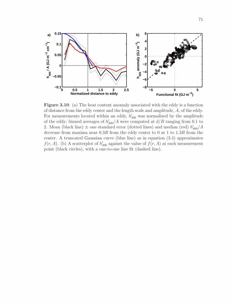
71

a) b)

0 0.5 1 1.5 2 2.5−0.1

−0.05

0

0.05

0.1

0.15

Normalized distance to eddy

h40

0′

/ A

(G

J m

−2 c

m−1

)

−5 0 5−8

−6

−4

−2

0

2

4

6

Functional fit (GJ m −2)

h40

0 ano

mal

y (G

J m

−2)

Figure 3.10: (a) The heat content anomaly associated with the eddy is a functionof distance from the eddy center and the length scale and amplitude, A, of the eddy.For measurements located within an eddy, h′

400was normalized by the amplitude

of the eddy; binned averages of h′400

/A were computed at d/R ranging from 0.1 to2. Mean (black line) ± one standard error (dotted lines) and median (red) h′

400/A

decrease from maxima near 0.3R from the eddy center to 0 at 1 to 1.3R from thecenter. A truncated Gaussian curve (blue line) as in equation (3.4) approximatesf(r, A). (b) A scatterplot of h′

400against the value of f(r, A) at each measurement

point (black circles), with a one-to-one line fit (dashed line).

72

0 0.05 0.1 0.15 0.2 0.25−600

−500

−400

−300

−200

−100

0

Peak amplitude of h ′z

0

/ A (GJ m −2 / cm)

z 0 (m

)

Figure 3.11: Peak amplitude of the functional fit (black x) computed as for Fig-ure 3.10 for depths between 0 and 600 m. The increase with depth is approximatedby an exponential curve (blue line) described by (0.33 × (1 − ez0/634)).

73

−1 −0.5 0 0.5 1−1.5

−1

−0.5

0

0.5

1

1.5

2

Σ he (GJ m−2)

H40

0′

(G

J m

−2)

Figure 3.12: A scatterplot of H′400

against the sum of heat content anomaliesdue to eddies (E). A linear regression (red dashed line) has a slope of 0.80±0.22.Uncertainties in E (gray lines) are computed as discussed in Section 3.7.

74

Table 3.1: The upper part of the table shows correlations of the transect-averagedupper-ocean heat content (H400) with average upper-ocean heat content north(HN) and south (HS) of the Polar Front and with the latitude of the Polar Front(φPF ), as well as the correlation of each variable with a two-harmonic fit to theseasonal cycle in each. The lower part of the table shows correlations of the residualheat content when a seasonal cycle has been removed (H′

400, H′

N , H′S) and φPF

with H′400

, φPF , the average heat flux anomaly upstream of Drake Passage 75 daysprior to a transect (Q75d, defined in Section 3.5) and heat content anomaly due tomesoscale eddies and meanders (E , defined in Section 3.6). Significant correlationsappear as bold text.

H400 HN HS φPF

H400 1 0.642 0.681 -0.591

seasonal cycle 0.705 0.552 0.833 .311

H′400

H′N H′

S φPF

H′400

1 0.506 0.292 -0.599

φPF -.599 0.037 0.025 1Q75d .416 0.147 0.101 -0.213

E 0.604 0.340 -0.065 -0.420

75

Table 3.2: Mean properties of eddies from the Chelton et al. (2011b) databaseintersected by an XBT transect: the number of each type of eddy (N), the averageamplitude (A), effective length scale (R) and latitude. Averages are computed overall warm- or cold-core eddies, or over eddies north or south of the Polar Front and± one standard error is reported for all quantities.

warm core total N of PF S of PFN 95 57 38A (cm) 14.4±1.0 18.2±1.2 8.6±1.1R (km) 79.3±2.3 84.6±2.7 71.3±3.8Lat. (◦S) 58.4±0.2 57.2±0.1 60.0±0.2cold core total N of PF S of PFN 90 18 72A (cm) -13.1±0.9 -15.8±1.7 -12.4±1.1R (km) 75.7±2.6 73.4±4.0 76.3±3.0Lat. (◦S) 59.1±0.2 56.7±0.2 59.7±0.2

76

Table 3.3: Averages of H400′ , H′N , and H′

S for all transects that intersected warm-or cold-core eddies and for transects that intersected warm- or cold-core eddiesnorth or south of the Polar Front. The displacement of the Polar Front (∆φPF ) iscomputed relative to the mean latitude of the Polar Front (58.5oS) over the 93 XBTtransects. Error bounds are one standard error, and bold values are significant atone standard error.

warm core All N of PF S of PFN 74 60 26H′

400(GJ m−2) 0.06±0.06 0.15±0.06 -0.17±0.09

H′N (GJ m−2) 0.14±0.07 0.23±0.08 -0.13±0.11

HS′ (GJ m−2) 0.00±0.04 −0.00±0.05 0.04±0.06∆φPF (km) -8±9 −18±9 14±17cold core All N of PF S of PFN 65 34 45H′

400(GJ m−2) -0.06±0.06 -0.08±0.08 -0.10±0.08

H′N (GJ m−2) 0.00±0.08 −0.24±0.11 0.10±0.10

HS′ (GJ m−2) 0.02±0.05 0.12±0.08 -0.04±0.05∆φPF (km) 5±9 -20±10 20±11

77

3.9 Acknowledgments

Data collection and analysis for this project was funded by NSF grants

to STG (ARRA OCE08050350) and JS (ANT0943818) and a NASA grant to

STG (NNX08AI82G). GRS would like to acknowledge a NASA Earth and Space

Science Fellowship and the ARCS Foundation for their support. STG acknowledges

sabbatical support from the French Centre National de la Recherche Scientifique.

NCEP Reanalysis 1 data were provided by the NOAA/OAR/ESRL PSD, Boulder,

Colorado, USA, from their Web site at http://www.esrl.noaa.gov/psd/.

Chapter III, in full, is a manuscript in preparation for publication. I was the

primary researcher and author of this material, with contributions from co-authors

Sarah Gille and Janet Sprintall.

Chapter 4

Subsurface melting of a

free-floating iceberg in the

Weddell Sea

78

79

4.1 Abstract

Observations near a large tabular iceberg in the Weddell Sea in March and

April 2009 show evidence that water from ice melting below the surface is dispersed

in two distinct ways. Warm, salty anomalies in T-S diagrams suggest that water

from the permanent thermocline is transported vertically as a result of turbulent

entrainment of meltwater at the iceberg’s base. Stepped profiles of temperature,

salinity, and density in the seasonal thermocline are more characteristic of double-

diffusive processes that transfer meltwater horizontally away from the vertical ice

face. These processes contribute comparable amounts of meltwater–O(0.1 m3)

to the upper 200 m of a 1 m2 water column–but only basal melting results in

significant upwelling of water from below the Winter Water layer into the seasonal

thermocline, suggesting that these two processes may have different effects on

vertical nutrient transport near an iceberg.

4.2 Introduction

Calving from glaciers in Antarctica accounts for 2,000 Gt of yearly fresh-

water input into the Southern Ocean, half of which takes the form of large tabular

icebergs (Jacobs et al., 1992). Icebergs with a major axis larger than 10 nautical

miles are responsible for most of the transport of freshwater north of 63◦ S (Silva

et al., 2006). Drifting icebergs redistribute heat and freshwater and transport trace

metals (Smith et al., 2007). Their effects on surface temperature and salinity alter

local stratification and may affect rates of sea-ice formation and Antarctic Bottom

Water formation (Jongma et al., 2009). Because icebergs tend to follow well-

defined tracks determined by prevailing winds and currents, they have enhanced

impacts on specific regions (Jenkins, 1999). For example, in regions with high

iceberg concentrations, such as the Weddell Sea, iceberg meltwater can contribute

as much to the freshwater balance as precipitation minus evaporation (Silva et al.,

2006).

Recent studies have shown that the wake of an iceberg is associated with an

increase in surface chlorophyll concentration (Schwarz and Schodlok, 2009). Melt-

80

ing ice contains biologically important micronutrients such as iron (Lin et al., 2011)

and may be enriched in nitrate and nitrite (Vernet et al., 2011). Concentrations

of other nutrients, such as phosphate and silicate, generally increase with depth

in the Weddell Sea (Vernet et al., 2011; Neshyba, 1977). Icebergs can therefore

increase nutrient supply near the surface directly in their meltwater (Smith et al.,

2007), or by melting at their base that entrains deep water and causes it to upwell

(Neshyba, 1977). There has been considerable debate, however, concerning the

location where most melting occurs, the vertical displacement of meltwater, and

the amount of ambient water entrained by upwelling meltwater.

Donaldson (1978) summarized three possibilities for meltwater distribution

from ice melting below the ocean surface. First, if little entrainment of surrounding

water occurs, meltwater will rise in a relatively thin layer and spread horizontally

at the surface as a lens of freshwater. Cooling and freshening of surface water near

an iceberg is discussed by Helly et al. (2011a). Second, meltwater that entrains

a large amount of ambient water from below the permanent thermocline can rise

and appear as a T-S anomaly higher in the water column. Such anomalies have

been observed near Pine Island Glacier (Jenkins, 1999). Third, meltwater can

spread horizontally in stratified layers, resulting in steps in hydrographic profiles.

These steps are a common feature of profiles in the Weddell Sea (Huppert and

Turner, 1980, hereafter HT80) and have also been measured near the edge of the

Erebus Glacier Tongue (Jacobs et al., 1981) and near an iceberg frozen into fast

ice (Ohshima et al., 1994).

Here, we present evidence for upwelled meltwater mixtures and horizontal

motion of meltwater in stratified layers observed near a free-floating iceberg in

the Weddell Sea. These two types of melting are identified in T-S diagrams and

potential density profiles and their freshwater contributions to the ocean near the

iceberg are estimated.

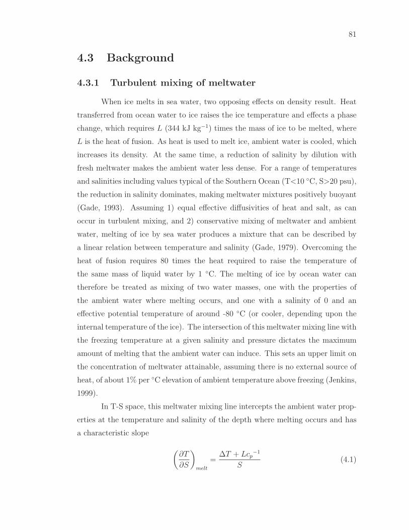
81

4.3 Background

4.3.1 Turbulent mixing of meltwater

When ice melts in sea water, two opposing effects on density result. Heat

transferred from ocean water to ice raises the ice temperature and effects a phase

change, which requires L (344 kJ kg−1) times the mass of ice to be melted, where

L is the heat of fusion. As heat is used to melt ice, ambient water is cooled, which

increases its density. At the same time, a reduction of salinity by dilution with

fresh meltwater makes the ambient water less dense. For a range of temperatures

and salinities including values typical of the Southern Ocean (T<10 ◦C, S>20 psu),

the reduction in salinity dominates, making meltwater mixtures positively buoyant

(Gade, 1993). Assuming 1) equal effective diffusivities of heat and salt, as can

occur in turbulent mixing, and 2) conservative mixing of meltwater and ambient

water, melting of ice by sea water produces a mixture that can be described by

a linear relation between temperature and salinity (Gade, 1979). Overcoming the

heat of fusion requires 80 times the heat required to raise the temperature of

the same mass of liquid water by 1 ◦C. The melting of ice by ocean water can

therefore be treated as mixing of two water masses, one with the properties of

the ambient water where melting occurs, and one with a salinity of 0 and an

effective potential temperature of around -80 ◦C (or cooler, depending upon the

internal temperature of the ice). The intersection of this meltwater mixing line with

the freezing temperature at a given salinity and pressure dictates the maximum

amount of melting that the ambient water can induce. This sets an upper limit on

the concentration of meltwater attainable, assuming there is no external source of

heat, of about 1% per ◦C elevation of ambient temperature above freezing (Jenkins,

1999).

In T-S space, this meltwater mixing line intercepts the ambient water prop-

erties at the temperature and salinity of the depth where melting occurs and has

a characteristic slope

(

∂T

∂S

)

melt

=∆T + Lcp

−1

S(4.1)

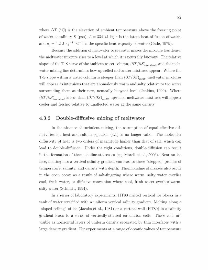
82

where ∆T (◦C) is the elevation of ambient temperature above the freezing point

of water at salinity S (psu), L = 334 kJ kg−1 is the latent heat of fusion of water,

and cp = 4.2 J kg−1 ◦C−1 is the specific heat capacity of water (Gade, 1979).

Because the addition of meltwater to seawater makes the mixture less dense,

the meltwater mixture rises to a level at which it is neutrally buoyant. The relative

slopes of the T-S curve of the ambient water column, (∂T/∂S)ambient, and the melt-

water mixing line determines how upwelled meltwater mixtures appear. Where the

T-S slope within a water column is steeper than (∂T/∂S)melt, meltwater mixtures

will appear as intrusions that are anomalously warm and salty relative to the water

surrounding them at their new, neutrally buoyant level (Jenkins, 1999). Where

(∂T/∂S)ambient is less than (∂T/∂S)melt, upwelled meltwater mixtures will appear

cooler and fresher relative to unaffected water at the same density.

4.3.2 Double-diffusive mixing of meltwater

In the absence of turbulent mixing, the assumption of equal effective dif-

fusivities for heat and salt in equation (4.1) is no longer valid. The molecular

diffusivity of heat is two orders of magnitude higher than that of salt, which can

lead to double-diffusion. Under the right conditions, double-diffusion can result

in the formation of thermohaline staircases (eg. Morell et al., 2006). Near an ice

face, melting into a vertical salinity gradient can lead to these “stepped” profiles of

temperature, salinity, and density with depth. Thermohaline staircases also occur

in the open ocean as a result of salt-fingering where warm, salty water overlies

cool, fresh water, or diffusive convection where cool, fresh water overlies warm,

salty water (Schmitt, 1994).

In a series of laboratory experiments, HT80 melted vertical ice blocks in a

tank of water stratified with a uniform vertical salinity gradient. Melting along a

“sloped ceiling” of ice (Jacobs et al., 1981) or a vertical wall (HT80) in a salinity

gradient leads to a series of vertically-stacked circulation cells. These cells are

visible as horizontal layers of uniform density separated by thin interfaces with a

large density gradient. For experiments at a range of oceanic values of temperature

83

and salinity, HT80 derived an empirical equation for layer thickness, h,

h =0.65 [ρ(Tfp, S) − ρ(T, S)]

∂ρ∂z

, (4.2)

where density, ρ, is a function of the depressed freezing point near the ice, Tfp, the

unperturbed salinity, S, and the unperturbed temperature, T .

Each circulation cell draws in ambient, unperturbed water near the top

of the cell (Malki-Epshtein et al., 2004). This water cools near the ice face, is

freshened slightly by entrainment of meltwater, and flows out near the bottom of

the cell. As water flows out, it is warmed by thermal diffusion across the lower

interface and rises slightly. Water flowing in along the tops of cells is cooled in a

similar fashion, giving a tilt to the isopycnal layers. Most of the meltwater coming

off the ice ends up vertically displaced to 2-3 layer thicknesses above where it

formed (Malki-Epshtein et al., 2004).

In this paper, we use equation (4.1) to identify water in T-S diagrams

and equation (4.2) to identify water in density profiles that has been influenced

by two modes of melting (turbulent or double-diffusive, respectively). We then

estimate where each type of melting occurs and gauge the amount of contributed

meltwater and the direction (vertical or horizontal) of transport. Our ultimate

goal is to understand the implications of iceberg meltwater for nutrient transport

and biological productivity.

4.4 Data and Methods

In March and April 2009, a cruise on the RV/IB Nathaniel B. Palmer (NBP)

to the Powell Basin (Fig. 4.1) in the Weddell Sea east of the Antarctic Peninsula

was undertaken to assess the impacts of icebergs on their biological, chemical,

and physical environment. The main object of study was a large tabular iceberg

designated C-18a. The iceberg C18 calved from the Ross Ice Shelf in 2002; C-18a is

a fragment of C18 that has been tracked by satellite since 2005 (Stuart and Long,

2011). Helly et al. (2011a) estimated the size of C-18a at about 35 km by 6 km

with an average height above the water line of 28 m. During the cruise, Sherlock

84

et al. (2011) used a remote operated vehicle (ROV) to examine the subsurface face

of C-18a directly. The maximum depth of ice recorded by a sonar onboard the

ROV was 190 m. Since melting is likely to be greater at the edge of the iceberg,

where this measurement was taken, the base of C-18a may have been deeper closer

to the center of the iceberg. C-18a travelled about 200 km from March 9 to April 1,

following a clockwise path around the Powell Basin (Fig. 4.1b). The approximate

position of C-18a was estimated from a combination of the ship’s location while

circumnavigating the iceberg, position fixes from the navigational radar of the

NBP, and interpolation in time and space when no direct measurements were

available.

This paper focuses on temperature and salinity profiles from 65 CTD casts

taken over the course of the cruise. Results from measurements of Fe and other

nutrients are reported elsewhere in this issue (Lin et al., 2011; Vernet et al., 2011).

Sampling centered around C-18a followed the same general trajectory as the iceberg

(Fig. 4.1b), resulting in CTD casts spread across the basin, divided here into four

regions : I. March 10-17 (red), II. March 18-22 (blue), III. March 29 - April 2

(green). IV. April 10-11 (magenta). Of the 65 CTD casts performed during the

cruise, 56 were deeper than 250 m, with most of these profiles going deeper than

500 m. Of the 56 casts deeper than 250 m, 37 occurred within 20 km of C-18a.

Of those 37 casts, 23 were between 0.4 and 2 km from the iceberg and 14 were

between 2 and 20 km from C-18a. In a region commonly referred to as “Iceberg

Alley” (IA, orange) (Ballantyne, 2002; Schodlok et al., 2006), characterized by a

high concentration of small icebergs 15 m to 2 km in length, sampling occurred

April 4-9 and included 12 CTD casts deeper than 250 m. An additional 7 CTD

profiles collected outside of IA and farther than 50 km from C-18a at the time of

survey occurred March 29 and April 3-7; these casts are grouped together (cyan).

4.5 Water masses of Powell Basin

Three main water masses—Warm (or Weddell) Deep Water (WDW), Win-

ter Water (WW), and Antarctic Surface Water (AASW)—comprise the upper 500

85

m of the water column in Powell Basin (Fig. 4.2). Around 500 m, water prop-

erties are characteristic of WDW, with a temperature of 0.5 ◦C and salinity of

34.6 psu (Solomon et al., 2000). This water mass, a form of Circumpolar Deep

Water that is cooled in the Weddell Gyre (Orsi et al., 1993; Rutgers van der

Loeff, 1994), varies little across the basin. In the permanent thermocline above

the WDW, both temperature and salinity increase with increasing depth with a

slope of around 6 ◦C psu−1. A temperature minimum, also known as the WW, is

found in the remnant of the winter mixed layer. Temperature in the WW shows

regional variability, with a general decrease to the south, reaching a minimum

around -1.7 ◦C (region IA), compared to -1.3 ◦C in the north (region III), but all

temperature minima occupy a relatively narrow salinity range around 34.4 psu.

In the seasonal thermocline, above the WW layer, temperature increases while

salinity decreases with a slope ranging from -1.25 ◦C psu−1 in IA to -4 ◦C psu−1 in

regions II and III. Surface water properties range from -1 ◦C in IA to 0.5 ◦C near

regions II and III with surface salinities near ∼33.8-33.9 psu.

The three water masses (WDW, WW, and AASW) form end members to a

typical CTD profile in Powell Basin, with the seasonal and permanent thermoclines

describing a “V” in T-S space. Deviations from a V-shape occurred in casts taken

near the sill separating Powell Basin from the Scotia Sea (Fig. 4.2, blue), where

large intrusions characteristic of interleaving water masses occur in the surface

layer above the temperature minimum, suggesting that bathymetry or advection

of water from the Scotia Sea may influence general water properties.

4.6 Results and Discussion

A series of five casts taken over 6 hours on a transect from 0.85 to 8.96 km

west of C-18a shows a clear impact of ice melt on the subsurface water column

(Fig. 4.3). Over the 8 km of the transect, the WW layer, marked in red in the

left-most, closest cast (Fig. 4.3), decreases in thickness from 150 m to 50 m. The

average salinity at 50 to 300 m depth increases with distance from C-18a. Cooler,

fresher water near the iceberg suggests the presence of meltwater. To examine the

86

source of this meltwater, we first examine T-S anomalies consistent with meltwa-

ter that is turbulently mixed at depth and upwelled. We then characterize the

thermohaline steps that indicate melting along a vertical ice face into a salinity

gradient. Finally, we make an approximate calculation of the amount of meltwater

attributable to each process.

4.6.1 A meltwater estimate from turbulent processes

Although the thick, well-mixed layer in the profile nearest C-18a in Fig-

ure 4.3 (WW marked in red) is cooler and fresher than water at the same depth

in the other casts from the transect, when T-S properties are compared along

isopycnals, this cast appears anomalously warm and salty (Fig. 4.4a). We use the

T-S curve from this cast to illustrate our method for estimating the amount and

concentration of meltwater in the vertical profiles due to turbulent basal melting

(Fig. 4.4b).

To identify water within the warm, salty anomaly, two local temperature

minima (points a and b in Figure 4.4b) are selected to define the line L2, where

L2 is a linear approximation to the “unperturbed” T-S relation. Points on the

observed T-S curve between a and b are therefore anomalously warm and salty

relative to L2. Points a and b also define the vertical extent of the warm intrusion;

for the cast shown in Figure 4.4b, they correspond to the depth range from (a)

84 m to (b) 97 m.

For mixing to produce water with the T-S properties of this anomaly re-

quires the upward displacement of warm, salty water from below the WW layer.

We expect melting at the base of the iceberg to produce fresh, cold water. If this

water mixes turbulently with ambient water, the resulting water will have a tem-

perature that falls along a line of slope (∂T/∂S)melt, defined by equation (4.1). The

right-hand side of equation (4.1) is calculated using the temperature and salinity

data for each cast. The mean value of (∂T/∂S)melt over the upper 300 m of a

profile is then used as the slope of the meltwater mixing line, L1. For the exam-

ple shown in Figure 4.4b, the mean value of (∂T/∂S)melt over this depth range is

2.36 ± 0.05 ◦C psu−1, where the uncertainty is computed as twice the standard

87

deviation of (∂T/∂S)melt over the upper 300 m. In equation (4.1), changes in ∆T

and S are small relative to L and the mean value of S, so variations in (∂T/∂S)melt

are small.

The meltwater mixing line, L1, serves as an upper bound to the anomalous

T-S region found between a and b. A line with slope (∂T/∂S)melt can pass through

each point in the anomaly between a and b. Here we choose the line L1 that is

tangent to the T-S anomalies such that the intercept at S = 0 occurs at the

maximum possible value for T . For the intrusion between a and b in the cast

shown in Figure 4.4b, the meltwater line L1 is defined by:

T (S) = (2.36 ± 0.05) × S − 82.4 ± 0.2, (4.3)

where T has units of ◦C and S is the salinity. The uncertainty in the intercept

is twice the standard deviation of all possible T -intercept values for lines passing

through the T − S points between a and b.

The minimum temperature and salinity required for basal melting to pro-

duce the observed anomaly occurs where L1 intersects the ambient T-S curve at

point c (Fig. 4.4b). Point c defines the location in the permanent thermocline

where the absolute value of the temperature difference between the ambient T-S

curve and the T-S values defined by L1 is a minimum. Uncertainties in the temper-

ature and salinity at point c (Tc and Sc) are estimated by propagating uncertainties

in the equation for L1 to the intersection point c. The depth of point c then defines

the minimum source depth, Zsource, of the upwelled meltwater. The uncertainty in

Zsource is estimated as the uncertainty in Tc divided by the mean ∂T/∂z calculated

over a 20 m depth range centered at Zsource. In the case shown in Figure 4.4b,

Tc = -1.02 ± 0.18 ◦C, Sc = 34.50 ± 0.04 psu and Zsource = 253 ± 20 m.

To estimate the amount of meltwater contained in the anomalous T-S region

between a and b, we consider water properties along L1 as a dilution of the ambient

water at c. Thus, the concentration of meltwater, M , is determined by

M(S) =Sc

S− 1, (4.4)

where S is the salinity along L1. In Figure 4.4b, for the small range of S (34.36-

34.43 psu) for which intrusions occur, M ranges from 0.20-0.41%. The uncertainty

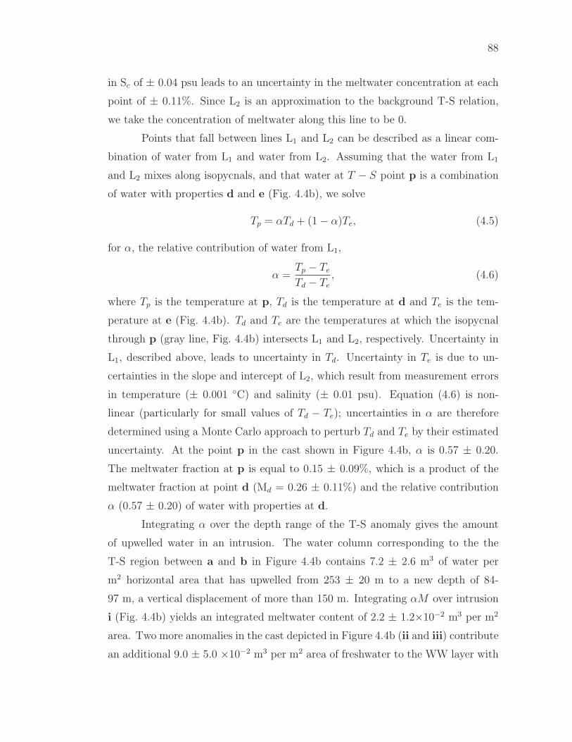
88

in Sc of ± 0.04 psu leads to an uncertainty in the meltwater concentration at each

point of ± 0.11%. Since L2 is an approximation to the background T-S relation,

we take the concentration of meltwater along this line to be 0.

Points that fall between lines L1 and L2 can be described as a linear com-

bination of water from L1 and water from L2. Assuming that the water from L1

and L2 mixes along isopycnals, and that water at T − S point p is a combination

of water with properties d and e (Fig. 4.4b), we solve

Tp = αTd + (1 − α)Te, (4.5)

for α, the relative contribution of water from L1,

α =Tp − Te

Td − Te

, (4.6)

where Tp is the temperature at p, Td is the temperature at d and Te is the tem-

perature at e (Fig. 4.4b). Td and Te are the temperatures at which the isopycnal

through p (gray line, Fig. 4.4b) intersects L1 and L2, respectively. Uncertainty in

L1, described above, leads to uncertainty in Td. Uncertainty in Te is due to un-

certainties in the slope and intercept of L2, which result from measurement errors

in temperature (± 0.001 ◦C) and salinity (± 0.01 psu). Equation (4.6) is non-

linear (particularly for small values of Td − Te); uncertainties in α are therefore

determined using a Monte Carlo approach to perturb Td and Te by their estimated

uncertainty. At the point p in the cast shown in Figure 4.4b, α is 0.57 ± 0.20.

The meltwater fraction at p is equal to 0.15 ± 0.09%, which is a product of the

meltwater fraction at point d (Md = 0.26 ± 0.11%) and the relative contribution

α (0.57 ± 0.20) of water with properties at d.

Integrating α over the depth range of the T-S anomaly gives the amount

of upwelled water in an intrusion. The water column corresponding to the the

T-S region between a and b in Figure 4.4b contains 7.2 ± 2.6 m3 of water per

m2 horizontal area that has upwelled from 253 ± 20 m to a new depth of 84-

97 m, a vertical displacement of more than 150 m. Integrating αM over intrusion

i (Fig. 4.4b) yields an integrated meltwater content of 2.2 ± 1.2×10−2 m3 per m2

area. Two more anomalies in the cast depicted in Figure 4.4b (ii and iii) contribute

an additional 9.0 ± 5.0 ×10−2 m3 per m2 area of freshwater to the WW layer with

89

91.6 ± 29.0 m3 of water upwelled from 246 ± 2 m into the depth range 97-240 m.

This estimate of the amount of water upwelled due to meltwater injection at the

base of the iceberg is sufficient to explain the 100 m increase in WW layer thickness

in this cast relative to casts farther away (Fig. 4.3).

Meltwater intrusions similar to that shown in Figure 4.4b were identified in

11 of the 23 casts closer than 2 km to C-18a, in 5 of the 12 casts in Iceberg Alley,

and in 1 cast 17 km from C-18a (Table 4.1). These T-S anomalies are smaller

than the large excursions hypothesized as due to water mass interleaving found in

casts near the sill to the northwest of Powell Basin (see for example blue casts in

Fig. 4.2). The slopes of the T-S anomalies due to meltwater intrusions are generally

close to the ∼2.4 ◦C psu−1 typical of meltwater mixing lines. Their appearance

in casts close to icebergs and absence in casts in the same region but farther from

icebergs suggest a local source. Most meltwater intrusions were found in region I

(Fig. 4.1b, red). The meltwater intrusion identified in the cast 17 km from C-18a

may be associated with a smaller iceberg observed in the vicinity at the time of

the CTD cast.

A summary of the depth range of meltwater intrusions observed in these

casts, the associated volume of meltwater and upwelled water, and the estimated

source depth of meltwater is presented in Table 4.1. Warm, salty anomalies in T-S

diagrams occurred primarily within the WW layer and at the base of the seasonal

thermocline. For casts closer than 2 km to C-18a, the anomalies occurred over a

range of depths from 67 m to 240 m, although the typical vertical extent of melt-

water intrusions was ∼27 m. Three casts that were less than 1 km from C-18a

showed multiple meltwater intrusions within one profile. Estimates of Zsource from

casts within 2 km from C-18a ranged from 163-305 m, with a median depth of

∼233 m, consistent with the iceberg keel depth of at least 190 m from direct ob-

servations (Helly et al., 2011a). In Iceberg Alley, which was populated by icebergs

much smaller than C-18a, intrusions occurred in a narrower depth range of about

76-158 m (Table 4.1) and were typically ∼25 m thick. Estimates of Zsource for the

cast 17 km from C-18a and casts in IA were generally much shallower than those

near C-18a, ranging from 124-164 m, at a median depth of ∼138 m (Table 4.1).

90

Smaller icebergs in IA are likely to have shallower keels than C-18a, consistent

with these estimates of meltwater source depth.

The apparent source depth of meltwater intrusions near C-18a showed de-

pendence on the position of a cast relative to fixed points on the iceberg. Although

C-18a rotated and translated over the course of the study, when CTD cast loca-

tions are considered relative to the iceberg’s major axis, a pattern emerges. To

describe these variations, we use a north-south orientation of the iceberg’s major

axis (as depicted near region I, Fig. 4.1b) to describe the positions of CTD casts

with meltwater intrusions (Table 4.1). Beginning with casts near the northwestern

tip of C-18a and moving counter-clockwise, estimates of Zsource ranged from 270-

305 m, decreased to 228-253 m at the midpoint of the iceberg’s long edge and had

a minimum of 163 m near the southern tip. Continuing counter-clockwise from

the southern tip, Zsource increased to 180-213 m at the midpoint of the iceberg’s

eastern edge and to 240 m in casts taken near the northeast corner of C-18a. These

variations in source depth may indicate that the northwest side of C-18a (in the

north-south orientation depicted near region I) was thicker than the southeast side.

These differences in thickness could have originated before C-18 initially calved,

as a result of melting at the seaward edge of the iceshelf. Enhanced melting along

the leading edge of the iceberg, ahead of the iceberg’s direction of motion, could

also lead to preferential thinning along that side of the iceberg.

Variations in Zsource could also result from variations in the depth of the

permanent thermocline. We have assumed that each cast is representative of the

conditions where melting occurs, but as Figure 4.3 shows, the permanent ther-

mocline may shoal with distance from C-18a. Because water at a given source

temperature and salinity is likely to be shallower in a cast farther from C-18a than

in a closer cast, shallower estimates of Zsource may simply reflect differences in

thermocline depth with distance from the iceberg. Thermocline depth may also

vary with position around the iceberg, reflecting varying degrees of impact by the

iceberg on water ahead or behind the direction of motion of the iceberg. Water

ahead of the iceberg’s leading edge may be less influenced by meltwater (although

it contains upwelled intrusions), have a shallower permanent thermocline, and as

91

a result produce shallower estimates of Zsource.

The volume of meltwater in any one profile due to these upwelled intrusions

spanned an order of magnitude from 0.6-13.5 ×10−2m3 per m2 (Table 4.1). The

volume of upwelled water was also highly variable, and was 2-3 orders of magnitude

higher than the volume of meltwater, reflecting the low concentrations of meltwa-

ter within an intrusion. In a typical meltwater intrusion near C-18a, O(10 m3)

water from the permanent thermocline is vertically displaced by O(100 m). Larger

volumes of meltwater and upwelled water occurred in those casts less than 2 km

from C-18a, where the median meltwater content in an intrusion was ∼2.8×10−2m3

per m2 horizontal area and the median volume of upwelled water was ∼11.3 m3,

displaced vertically by ∼93 m. Farther from C-18a and in IA, the volume of melt-

water in a typical intrusion was ∼1 ×10−2m3 per m2, with an associated ∼8.7 m3

per m2 of water in the permanent pycnocline displaced ∼30 m upwards.

An intermittent physical mechanism for these meltwater intrusions could

explain their localization and the variability of their meltwater content. If meltwa-

ter at the base of an iceberg is well-mixed, it would produce a less dense mixture

of meltwater whose upward motion is constrained by the keel of the iceberg. This

positively buoyant water would occasionally “spill” upwards from the edge of the

iceberg and rise to a depth at which it is neutrally buoyant. Mixing with wa-

ter as it rises or at its new density level would move the T-S properties away

from the meltwater mixing line, resulting in T-S anomalies whose core has a slope

near 2.4◦C psu−1 and whose sides relax towards the ambient T-S curve. Several

discrete upwelling events like this could explain the casts that exhibited multiple

intrusions; such an intermittent mechanism would also explain why many casts

close to icebergs did not display these intrusions and why such a large range of

upwelled volumes was observed.

4.6.2 A meltwater estimate from double-diffusive processes

Melting along the vertical sides of an iceberg is a second source of freshwater

that can ultimately be entrained into horizontally stratified layers. Unlike the

intrusions associated with upwelled basal meltwater, these layers are not evident

92

in T-S diagrams, but are instead visible as steps in profiles of temperature, salinity,

and density. As an example, steps are evident in profiles of potential density in two

casts taken an hour apart at distances 0.4 km (Fig. 4.5a, left) and 1.3 km (Fig. 4.5a,

right) from C-18a on 22 March 2009 (at 51.59◦ W, 61.68◦ S and 51.59◦ W, 61.67◦ S,

respectively, blue in Fig. 4.1b). These thermohaline steps possess several of the

qualities found in laboratory studies (HT80). One expected feature of layers formed

by sidewall melting in a salinity gradient is an upward tilt away from the cooling

source (HT80; Malki-Epshtein et al., 2004). In both casts in Figure 4.5a, steps

appear at the same potential densities, but are displaced upwards by ∼12 m in

the more distant cast (Fig. 4.5a, right), suggesting that layers are coherent over

a distance of at least 0.9 km. The two casts shown in Figure 4.5 confirm that

isopycnals slope upwards away from the ice face, as suggested by HT80. Another

expected feature of the circulation cells is freshening with depth within a layer due

to entrainment of meltwater into the outward-flowing circulation (HT80; Malki-

Epshtein et al., 2004). Here we find negative values of the salinity gradient with

depth, ∂S/∂z, occur over short depth intervals within a generally positive salinity

gradient (eg. at 113-115 m depth in Fig. 4.5b, Table 4.2), showing evidence of

local freshening.

The circulation cells set up by double-diffusion at an ice face consist of

layers of uniform density, bounded above and below by interfaces, where strong

gradients occur. To identify possible interfaces in the 56 CTD casts deeper than

250 m, we determined local maxima in the vertical gradient of potential density,

∂σ/∂z, (points f and m in Fig. 4.5b). We considered only points where ∂σ/∂z

exceeded a threshold of 4×10−3 kg m−3 dbar−1, approximately twice the mean

of ∂σ/∂z over the upper 300 m of casts close to C-18a. Furthermore, a layer

was identified only if the minimum value of ∂σ/∂z (q in Fig. 4.5b) between two

adjacent interfaces was at least 4×10−3 kg m−3 dbar−1 smaller than ∂σ/∂z at both

interfaces (f and m in Fig. 4.5b). Use of a smaller threshold increased the number

of layers identified as steps and resulted in smaller average step sizes. A larger

threshold had the opposite effect, finding fewer, larger steps. However, varying the

threshold by 1×10−3 kg m−3 dbar−1, resulted in no significant change in estimates

93

of the salinity deficit, nor in the resulting freshwater estimate associated with

the steps. In some instances where potential density gradients were small, such as

below ∼150 m, the use of the 4×10−3 kg m−3 dbar−1 threshold caused two or more

step-like features separated by a weak gradient to be counted as one layer. Prior

studies (eg Jacobs et al., 1981; Ohshima et al., 1994) that observed small steps

embedded in larger steps identified the main layers with the stronger gradients as

steps; where such steps occurred, we have done likewise.

The thickness of a layer bounded by the two interfaces (f and m in Fig. 4.5b)

is measured from the bottom of the upper interface (g) to the bottom of the lower

interface (n). The bottom (g or n) of an interface (f or m) is identified as the

shallowest local minimum in ∂2σ/∂z2 where ∂σ/∂z is less than the mean potential

density gradient between the two interfaces (f or m). Given the 1 m resolution of

the CTD data, the minimum observable layer thickness with this method is 2 m.

In the upper 300 m of the 56 CTD casts considered, 850 layers were iden-

tified using this methodology. In Table 4.2 we compare step properties for casts

at different distances from the iceberg: closer than 2 km from C-18a; in a range

2-20 km from C-18a; in IA (orange, Fig. 4.1b); and in casts far from ice (cyan

in Fig. 4.1b). Typically, ∼15 layers were found in each cast, irrespective of dis-

tance from the iceberg. Layers were characterized by average changes in temper-

ature of approximately -0.05 ◦C, changes in potential density of approximately

0.023 kg m−3, and salinity changes of approximately 0.027 psu on average, ex-

cept in IA which had larger salinity and density changes and smaller temperature

changes (Table 4.2). Layers most commonly appeared above the WW with a mean

depth of ∼84 m, except in IA where the mean depth of the isopycnal layers was

∼57 m (Table 4.2). The mean layer thickness agreed within two standard errors,

ranging from 7.3 ± 7.9 m in the casts far from the iceberg (C in Fig. 4.1b) to

9.1 ± 6.3 m for those casts less than 2 km from C-18a. The average minimum

salinity gradient, ∂S/∂z, was weakly negative (∼-2.4 ± 2.0×10−3 psu m−1) for

those casts closer than 2 km to C-18a. Farther from C-18a and in IA, the average

minimum ∂S/∂z in a layer was not significantly different from zero. This suggests

that freshening with depth within a layer, a feature of circulation cells suggested

94

by HT80, is more evident in casts closer to C-18a.

To test the predictions of layer thickness made by HT80, we computed h

from equation (4.2) using the temperature and salinity from each cast and the

freezing temperature calculated using the salinity-pressure profile. Potential den-

sity was used in place of density in equation (4.2), and for each cast the vertical

gradient in potential density, ∂σ/∂z, was averaged with a 50-point running mean.

While the laboratory experiments of HT80 were performed in a uniform

density gradient and at constant temperature, the environment of the Weddell

Sea has neither of these features. Variations in salinity, temperature, and ∂σ/∂z

with depth (eg. Fig. 4.5a) lead to a vertically varying predicted layer thickness,

h (Fig. 4.6a). Predicted layer thickness reaches a minimum of about 2.5 m in the

temperature-minimum layer, where water as cool as -1.5 ◦C is already close to the

depressed freezing point (Fig. 4.5a).

For each step identified in the potential density profiles, the observed and

predicted layer thickness were binned by depth and averaged (Fig. 4.6b). Agree-

ment between observed and predicted layer thickness is best from 40 to 100 m

depth (Fig. 4.6b). In the surface mixed layer, air-sea heat flux and wind forcing

mix out any stratified step structure, resulting in very few layers being identified

in the upper 50 m. The resulting low stratifications in the surface mixed-layer

lead to a breakdown in equation (4.2). This suggests that, in the surface layer, the

dominant direction of meltwater motion is upwards, and also that double-diffusive

melting into stratified layers may not be a relevant mixing process in this part of

the water column.

Thicker layers observed below the temperature minimum (130-180 m in

Fig. 4.5a) could be due to merging of two or more smaller layers with distance

from the iceberg. Greater buoyancy of meltwater at depth results in meltwater

that rises more quickly, which could lead to thicker layers at greater depth. Below

the temperature minimum, water that is cool and fresh overlies warmer, saltier

water and diffusive convection can occur, rather than salt fingering, which may

also enhance layer thickness.

Following Jacobs et al. (1981), we estimate the amount of meltwater present

95

in the thermohaline steps by assuming that a salt deficit can be defined by the area

between the salinity-depth profile of a typical thermohaline step and a line drawn

tangent (R in Fig. 4.5b) between the bases of the two interfaces (g and m) that

define the step (dashed lines in Fig. 4.5b). Water at the tops of the circulation

cells (at g and m) is ambient water cooled slightly as it is drawn in towards the

ice; it has the salinity of the ambient water, making line R a linear approximation

to the background salinity profile.

Physically, we also assume that the observed steps are formed by the addi-

tion of freshwater to the water column and are not due to a rearrangement of T and

S within the water column. Where the water column is diffusively stable (warm,

fresh water over cool, salty water), as it is in the seasonal thermocline above the

WW layer, diffusive convection and salt-fingering do not occur, suggesting that

sidewall melting could be the predominant cause of the steps. The salinity deficit

for the case pictured in Figure 4.5b is 0.05 psu m, equivalent to a deficit of about

0.05 g cm−2 salt or the addition of 1.5×10−2m3 freshwater to a 1 m2 area of the

water column.

In casts closer than 2 km to C-18a (Table 4.2), steps with a mean (± 2

standard errors) salinity deficit of 0.042 ± 0.035 g cm−2 imply a freshwater excess

of 1.23 ± 1.03 cm per step. The amount of freshwater in layers at other sites agreed

within two standard error bars (Table 4.2), but the average freshwater excess in

a typical layer in IA was not significantly different from zero. Integrating the

freshwater excess over each cast, we find that the total freshwater contribution in

the upper 300 m of a 1 m2 water column due to sidewall melting is O(0.1-0.2 m3).

4.7 Conclusions

At least two modes of meltwater mixing appear to contribute freshwater

to the region near C-18a. Warm, salty anomalies appear primarily in CTD casts

taken less than 2 km from the iceberg. The amount of meltwater, the proximity

to the iceberg, and the close match in T-S space with the slope of the predicted

meltwater mixing line are consistent with upwelled mixtures of basal melt and

96

ambient water near the base of the iceberg. Upwelled basal meltwater is highly

variable in space, and appears to be localized; intrusions are detectable mostly

within about 2 km of the iceberg. Only half of the casts within 2 km of C-18a

exhibited these intrusions, suggesting that upwelling of meltwater mixtures may be

an intermittent process. Where basal melting occurs, it appears to be responsible

for O(0.1 m3) of freshwater in a 1 m2 water column. A small amount of ice is

melted, cooling and freshening a much larger volume of water from the permanent

thermocline. This water does not rise all the way to the surface, but instead finds

a neutrally buoyant level at the base of the seasonal thermocline, where it forms

a thick layer of water that, although slightly warmer than the ambient WW at

the same density, is cool relative to the AASW and WDW. This supports the idea

suggested by Jacobs et al. (1979) that icebergs may play a role in maintaining the

WW layer.

The highly variable nature of the upwelling basal meltwater mixtures may

contribute to the observed patchiness in micronutrient supply (Lin et al., 2011)

and in the phytoplankton (Vernet et al., 2011) and zooplankton (Kaufmann et al.,

2011) communities near C-18a. Vertical nutrient transport can stimulate primary

production, but the initial effect of a large injection of deeper water (from ∼200 m)

into the euphotic zone (estimated to be 50-100 m deep (Vernet et al., 2011)) is

likely to be a dilution of phytoplankton populations. This may be a factor in the

delay between passage of an iceberg and increased productivity in its wake (eg.

Schwarz and Schodlok, 2009; Helly et al., 2011a).

Thermohaline steps consistent with melting from a vertical ice face are

ubiquitous in profiles in this region, especially in the depth range 40-100 m. These

steps exhibit many of the properties of the meltwater layers observed in the tank

experiments of HT80. The average thickness of layers associated with steps in

the seasonal thermocline matches that predicted by equation (4.2). Layers appear

to be continuous over short distances and tilt upwards with distance from the

iceberg. Freshening towards the bottom of the steps is also observed. The amount

of freshwater contained in thermohaline steps within a 1 m2 water column is ∼0.1-

0.2 m3, similar to the estimated freshwater ascribed to upwelled basal meltwater

97

mixtures. This value is 2-3 times larger than the 0.06 m3 per m2 that Jacobs et al.

(1981) observed near the Erebus Glacier Tongue, where conditions were much

cooler.

The appearance of these steps in all of the casts we examined, even far from

ice, and in a diffusively-stable part of the water column suggests that they are sta-

ble and that the influence of melting ice is discernible across the Powell Basin.

Horizontal spread of meltwater and associated nutrients by double-diffusive circu-

lation cells provides a means by which the seasonal thermocline can be enriched

in nutrients from ice melt over a much larger area than turbulent upwelling with-

out diluting microbial and planktonic populations. Near an ice face, where ice is

actively melting, advection by shear flow between cells could contribute to the for-

mation of thin, vertically-stacked layers in existing patches of plankton, and could

act to enhance horizontal dispersal of such patches.

This study confirms that both basal and sidewall melting contribute signifi-

cant amounts of freshwater to the upper ocean near icebergs. No single mechanism

dominates subsurface ice melt. Basal melt induces vertical transport of potentially

nutrient-rich water, while sidewall melting has the potential to enrich the thermo-

cline in micronutrients over a large areal extent. The data collected in this study

were not sufficient to characterize horizontal variations in subsurface meltwater

or the detailed advection of meltwater relative to the iceberg. These issues will

require further detailed field work.

98

a)

72oW 66oW 60oW 54oW 48oW 42 o

W

68oS

64oS

60oS

56oS

52oS

Depth (m

)

−6000

−5000

−4000

−3000

−2000

−1000

0

b)

52oW 51oW 50oW 49oW 48oW 63oS

40’

20’

62oS

40’

20’

61oS

−3000−3000

−3000

−3000

−3000

−3000

−3000

−2000

−2000

−2000

−2000

−1000

−1000

I

IIIII

IV

IA

C

Figure 4.1: (a) Powell Basin is in the northwest Weddell Sea, just east of DrakePassage and the Antarctic Peninsula, south of the Scotia Sea. (b) C-18a travelledclockwise around the Powell Basin; the estimated positions on March 11 (I), March22 (II), March 31 (III), and April 10 (IV) are indicated. CTD casts were collectednear C-18a on March 10-17 (red), March 18-22 (blue), March 29-April 2 (green),and April 10-11 (magenta). Sampling occurred in Iceberg Alley (IA, orange) April4-9. Outside of IA, casts that were more than 50 km from C-18a at the time ofsurvey are grouped together (cyan) and include casts taken April 3-7 at or en routeto a reference station (C) and one cast taken ∼74 km from C-18a on March 29(near III).

99

Figure 4.2: T-S curves for 56 CTD profiles are grouped by location and time andcolor-coded as in Fig. 4.1. CTD casts were collected near C-18a on March 10-17(red), March 18-22 (blue), March 29-April 2(green), April 10-11 (magenta), in Ice-berg Alley (orange), and far from ice (cyan). A seasonal thermocline lies betweenthe AASW and WW. A permanent thermocline separates WW from WDW.

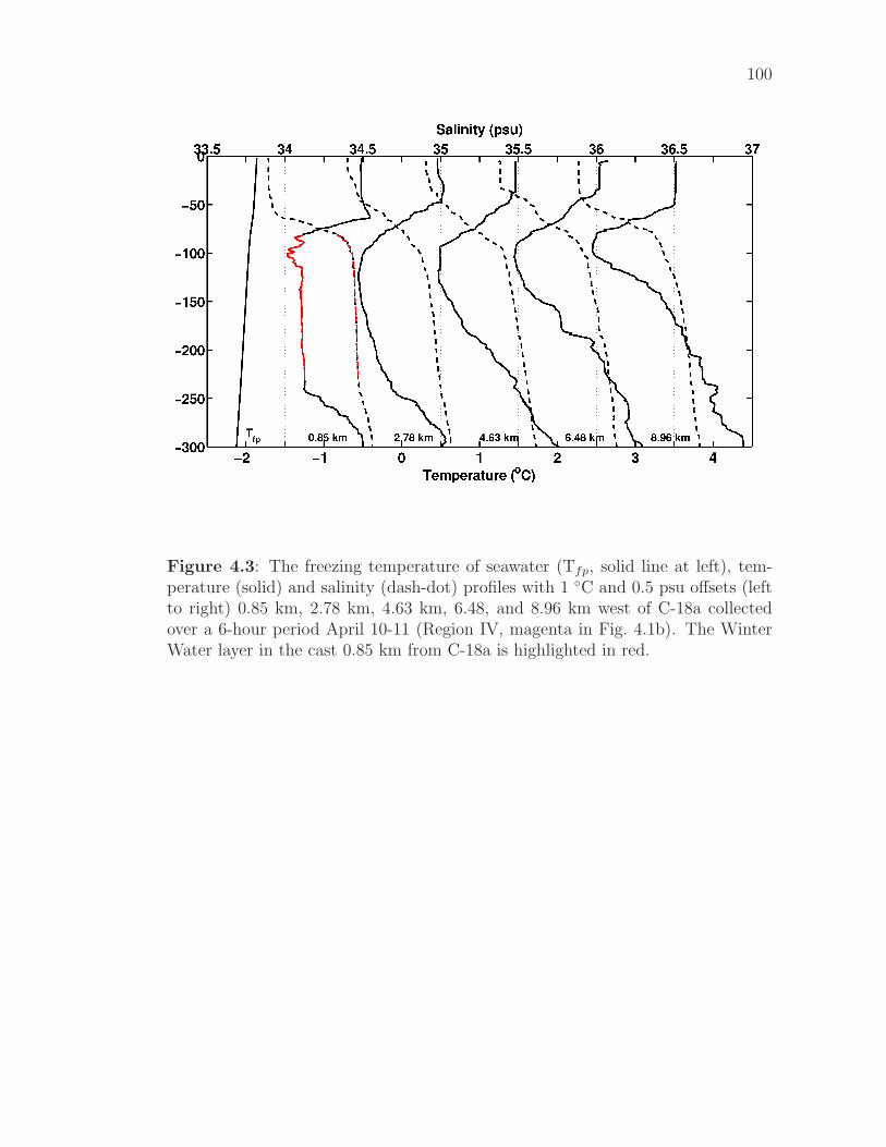
100

Figure 4.3: The freezing temperature of seawater (Tfp, solid line at left), tem-perature (solid) and salinity (dash-dot) profiles with 1 ◦C and 0.5 psu offsets (leftto right) 0.85 km, 2.78 km, 4.63 km, 6.48, and 8.96 km west of C-18a collectedover a 6-hour period April 10-11 (Region IV, magenta in Fig. 4.1b). The WinterWater layer in the cast 0.85 km from C-18a is highlighted in red.

101

a)

Salinity (psu)

Tem

pera

ture

(oC

)

33.8 34 34.2 34.4 34.6

−1.5

−1

−0.5

0

0.5

Figure 4.4: (a) T-S diagrams of casts taken 10-11 April (IV, magenta in Fig. 4.1).The cast 0.85 km from C-18a (see Fig. 4.3) shows warm and salty anomalies in thetemperature-minimum layer (red). (b) Expanded view of a warm, salty anomaly(i) bounded by points a and b, illustrating the meltwater estimation procedureoutlined in the text. A point p in the anomaly is modeled as an along-isopycnalmixture of water at d from the meltwater mixing line, L1, and water at e froma linear approximation to the ambient T-S relation, L2. The temperature andsalinity required for basal melting to produce the anomaly (i) occurs where L1

intersects the ambient T-S curve at c. Two additional anomalies (ii and iii) areevident in this cast.

102

a)

−3 −2 −1 0 1 2 3−400

−300

−200

−100

0

Temperature ( oC)

Dep

th (

m)

26.6 26.8 27 27.2 27.4 27.6 27.8

−400

−300

−200

−100

0

Potential Density (kg/m 3)

Dep

th (

m)

Temperatureσ

b)

−1.5 −1.4 −1.3 −1.2 −1.1−122

−120

−118

−116

−114

−112

−110

−108

−106

Temperature ( oC)

34.24 34.26 34.28 34.3 34.32

−122

−120

−118

−116

−114

−112

−110

−108

−106

Salinity (psu) or σ + offset (kg m −3)

R

f

m

g

n

q

Dep

th (

m)

Figure 4.5: (a) The freezing temperature (red line, left) and profiles of tempera-ture (red) and potential density (black) in two casts taken one hour apart 0.4 km(left) and 1.4 km (right) south of C-18a, March 22 (blue in Fig. 4.1b). The profileon the right is offset 2 ◦C and 0.2 kg m−3. Isopycnals (dotted line) slant upwardsaway from the ice in 50-100 m depth range, so that steps in temperature and po-tential density in the cast at 0.4 km are evident at the same potential densities inthe cast at 1.4 km, shifted vertically by ∼ 12 m. (b) Expanded view of a step intemperature (red), salinity (blue) and potential density (offset by -992.99 kg m−3)(black) in the cast 0.4 km from C-18a (left profile in (a)), illustrating the step-finding procedure outlined in the text. The interfaces at f and m have lower boundsat g and n, respectively, at depths indicated by the dotted lines. A minimum in∂σ/∂z is found at q. R is drawn tangent to the salinity/depth profile at the depthsof g and n. The area between R and the salinity-depth profile (blue line) definesthe salinity deficit.

103

a)

0 10 20 30 40 50−400

−300

−200

−100

0

Layer Thickness (m)

Dep

th (

m)

b)

0 10 20 30 40 50−250

−200

−150

−100

−50

0

Layer thickness (m)

Dep

th (

m)

observedpredicted

Figure 4.6: (a) Observed layer thickness (x) and layer thickness predicted fromequation (4.2) (solid line), calculated from temperature and salinity data for theprofile at 0.4 km in Fig. 4.5a. Layer thickness is at a minimum in the temperatureminimum layer and increases below 200 m. (b) Mean observed (red) and predicted(blue) layer thicknesses binned by depth for all layers identified in potential densityprofiles. Where layers were observed, predicted layer thickness (red) is calculatedas the average value of h in equation (4.2) over the depth range of the layer. Blacklines indicate standard error. Layer thickness agrees most closely in the 40-100 mdepth range, averaging about 5 m.

104

Table 4.1: Properties of meltwater intrusions in 11 casts closer than 2 km toC-18a, 1 cast 17 km from C-18a, and 5 casts in Iceberg Alley. The intrusion depthrange of the warm, salty T-S anomalies are indicated. Source depth of meltwatermixtures and the volumes (per m2 area) of meltwater and upwelled water in theintrusion are estimated as described for Figure 4.4b in the text. Error bars arecomputed as described in the text.

Cast#

Dist.to C-18a(km)

Region IntrusionDepth (m)

Zsource (m) Vol. Melt.(10−2 m3)

UpwelledVol. (m3)

19 0.4 II 130 to 154 270 ± 18 6.0 ± 2.5 11.2 ± 4.725 0.4 III 67 to 88 241 ± 7 4.8 ± 1.3 8.8 ± 4.72 0.6 I 83 to 135 234 ± 24 10.2 ± 4.5 19.2 ± 10.4

135 to 175 205 ± 7 3.3 ± 1.7 19.2 ± 7.39 0.6 I 72 to 77 163 ± 14 1.4 ± 0.5 2.7 ± 1.01 0.7 I 97 to 120 244 ± 6 2.6 ± 0.9 5.7 ± 5.5

120 to 150 231 ± 4 7.6 ± 2.0 21.6 ± 5.8150 to 189 220 ± 7 2.7 ± 1.1 11.5 ± 6.5

10 0.7 I 83 to 107 228 ± 20 2.7 ± 0.9 6.2 ± 4.265 0.85 IV 84 to 97 253 ± 20 2.2 ± 1.2 7.2 ± 2.6

97 to 101 241 ± 11 0.3 ± 0.2 2.0 ± 0.9101 to 240 246 ± 3 8.7 ± 4.8 89.6 ± 28.1

5 1.2 I 97 to 165 180 ± 7 5.3 ± 2.9 24.4 ± 11.530 1.7 III 202 to 208 305 ± 32 0.9 ± 0.5 1.9 ± 1.36 1.8 I 97 to 134 202 ± 7 4.6 ± 2.1 17.4 ± 6.816 1.8 II 136 to 182 213 ± 8 2.9 ± 1.2 12.8 ± 8.53 17.2 I 81 to 90 132 ± 5 0.6 ± 0.3 3.7 ± 2.241 – IA 76 to 98 145 ± 7 1.3 ± 0.7 6.9 ± 4.250 – IA 92 to 118 136 ± 3 1.1 ± 0.5 10.2 ± 4.551 – IA 82 to 106 124 ± 10 1.6 ± 0.7 9.8 ± 4.652 – IA 121 to 158 164 ± 2 0.7 ± 0.3 8.7 ± 7.155 – IA 96 to 117 125 ± 2 0.8 ± 0.3 8.7 ± 3.6

105

Table 4.2: Mean properties (± twice the standard error) of themohaline steps inprofiles of potential density from CTD casts less than 2 km from C-18a, between2 and 20 km from C-18a, in Iceberg Alley, and other casts far from ice. Thereported depth of a layer is the depth of its midpoint. Layer thickness is thedistance between the bases of the interfaces that define the layer. ∆σ, ∆T and ∆Sare the change in potential density, temperature, and salinity across a layer. Theminimum salinity gradient, ∂S/∂z, observed within each layer is averaged over thecasts in each group. The salinity deficit within a layer is computed as outlined inthe text. The freshwater excess is the amount of freshwater required to accountfor the integrated salinity deficit in each cast.

Profile Group < 2 km 2 to 20 km Iceberg Alley OtherNumber of Casts 23 14 12 7# of Layers per Cast 16.7±1.7 14.9±2.1 12.4±1.2 15.6±1.6Depth of Layers (m) 89.5±20.1 78.9±15.7 57.2±12.4 82.9±14.1Layer Thickness (m) 9.1±6.3 7.3±5.3 7.4±6.3 7.3±7.9∆σ (10−2 kg m−3) 2.2±0.9 2.3±0.8 3.1±1.0 2.5±0.9∆ T (10−2 ◦C) -5.4±4.7 -5.6±4.9 -2.1±6.0 -3.5±8.8∆ S (10−2 psu) 2.6±1.0 2.7±1.0 3.9±1.2 3.0±1.2Minimum of ∂S/∂z(10−3 psu m−1)

-2.4±2.0 -2.0±2.6 0.6±2.0 -1.9±2.6

Salinity deficit / step(10−2 g cm−2)

4.2±3.5 3.3±2.6 4.0±5.0 2.2±1.3

Freshwater excess /cast (10−2m3 per m2)

18.5±4.7 12.9±4.1 13.5±4.7 9.1±1.5

106

4.8 Acknowledgments

We are grateful to the staff from Raytheon Polar Services and the captain

and crew of the RV/IB Nathaniel B. Palmer for their support in the field. We

would also like to thank Yvonne Firing for her feedback during the manuscript

preparation. The field component of this research was funded by a NSF award to

M. Vernet (ANT - 0636730). Data analysis was funded by a NSF award to S. Gille

and J. Sprintall (NSF ARRA OCE0850350) and a NASA Earth and Space Science

Fellowship to G. Stephenson.

Chapter IV, in its entirety, is a reprint with no modifications to content of

the article as it appears in Deep-Sea Research II, 2011, G.R. Stephenson Jr., J.

Sprintall, S.T. Gille, M. Vernet, J.J. Helly, and R.S. Kaufmann, reproduced with

permission of Elsevier. I was the primary researcher and author of this manuscript.

Maria Vernet, John Helly, and Ron Kaufmann contributed to the field component

of the research which forms the basis of this chapter. Janet Sprintall and Sarah

Gille supervised the analysis and writing of the manuscript.

References

Alexander, M. A., and Deser, C., 1995: A mechanism for the recurrence ofwintertime midlatitude SST anomalies. J. Phys. Oceanogr., 25, 122137. doi:10.1175/1520-0485(1995)025<0122:AMFTRO>2.0.CO;2.

Ballantyne, J., 2002: A multidecadal study of the number of Antarctic ice-bergs using scatterometer data. Brigham Young University online report,http://www.scp.byu.edu/data/iceberg/IcebergReport.pdf.

Bindoff, N. L., and McDougall, T. J., 2000: Decadal changes along an Indian Oceansection at 32◦CS and their interpretation. J. Phys. Oceanogr., 30, 1207–1222.

Boe, J., Hall, A., and Qu, X., 2009: Deep ocean heat uptake as a majorsource of spread in transient climate change simulations. Geophys. Res. Let-

ters, 36(L22791). doi:10.1029/2009GL040845.

Boning, C. W., Dispert, A., Visbeck, M., Rintoul, S. R., and Schwarzkopf, F. U.,2008: The response of the Antarctic Circumpolar Current to recent climatechange. Nature Geoscience, 1, 864–869.

Bracegirdle, T. J., Connolley, W., and Turner, J., 2008: Antarctic climatechange over the twenty first century. J. Geophys. Res., 113(D03103),doi:10.1029/2007JD008933.

Brainerd, K. E., and Gregg, M. C., 1995: Surface mixed and mixing layers. Deep

Sea Res., 42, 1521–1543.

Caldeira, K., and Duffy, P. B., 2000: The role of the Southern Ocean in uptakeand storage of anthropogenic carbon dioxide. Science, 287, 620–622.

Chelton, D. B., Gaube, P., Schlax, M. G., Early, J. J., and Samelson, R. M., 2011a:The influence of nonlinear mesoscale eddies on oceanic chlorophyll. Science, 334,328–332.

Chelton, D. B., Schlax, M. G., and Samelson, R. M., 2011b: Global observationsof nonlinear mesoscale eddies. Prog. Oceanogr., 91, 167–216.

107

108

Church, J., Gregory, J., White, N., Platten, S., and Mitrovica, J., 2011: Under-standing and projecting sea level change. Oceanography, 24, 130–143.

Ciasto, L. M., and England, M. H., 2011: Observed ENSO teleconnections toSouthern Ocean SST anomalies diagnosed from a surface mixed layer heat bud-get. Geophys. Res. Lett., 38(L09701). doi:10.1029/2011GL046895.

Cunningham, S. A., Alderson, S. G., King, B. A., and Brandon, M. A., 2003:Transport and variability of the Antarctic Circumpolar Current in Drake Pas-sage. J. Geophys. Res.-Oceans, 108. doi:10.1029/2001JC001147.

de Boyer Montegut, C., Madec, G., Fischer, A. S., Lazar, A., and Iudicone, D.,2004: Mixed layer depth over the global ocean: An examination of profiledata and a profile-based climatology. J. Geophys. Res., 109(C12003). doi:10.1029/2004JC002378.

Deser, C., Alexander, M. A., and Timlin, M. S., 2003: Understanding the per-sistence of sea surface temperature anomalies in mid-latitudes. J. Climate, 16,57–72.

Donaldson, P. B., 1978: Melting of Antarctic icebergs. Nature, 275, 305–306.

Dong, S., Gille, S. T., and Sprintall, J., 2007: An assessment of the SouthernOcean mixed layer heat budget. J. Climate, 20, 4425–4442.

Dong, S., Sprintall, J., Gille, S. T., and Talley, L., 2008: Southern Ocean mixed-layer depth from Argo float profiles. J. Geophys. Res., 113(C6), C06013.

Durack, P. J., and Wijffels, S. E., 2010: Fifty-year trends in global ocean salinitiesand their relationship to broad-scale warming. J. Climate, 23, 4342–4362.

Fang, F., and Morrow, R., 2003: Evolution, movement and decay of warm-coreLeeuwin Current eddies. Deep-Sea Res. Part II., 50, 2245–2261.

Firing, Y. L., Chereskin, T. K., and Mazloff, M. R., 2011: Vertical structureand transport of the Antarctic Circumpolar Current in Drake Passage fromdirect velocity observations. J. Geophys. Res.-Oceans, 116(C08015). doi:10.1029/2011JC006999.

Gade, H. G., 1979: Melting of ice in sea water: A primitive model with applicationto the Antarctic ice shelf and icebergs. J. Phys. Oceanogr., 9, 189–198.

Gade, H. G., 1993: When ice melts in sea water: A review. Atmosphere-Oceans,31, 139–165.

Gille, S. T., 2008: Decadal-scale temperature trends in the Southern Hemisphereocean. J. Climate, 21, 4749–4765.

109

Gille, S. T., Lombrozo, A., Sprintall, J., Stephenson, G., and Scarlet, R., 2009:Anomalous spiking in spectra of XCTD temperature profiles. J. Atm. Oceanic

Technol., 26, 1157–1164.

Hall, A., and Visbeck, M., 2002: Synchronous variability in the Southern Hemi-sphere atmosphere, sea ice, and ocean resulting from the annular mode. J.

Climate, 15, 3043–3057.

Hanawa, K., Rual, P., Bailey, R., Sy, A., and Szabados, M., 1995: A new depth-time equation for Sippican or TSK T-7, T-6 and T-4 expendable bathythermo-graphs (XBT). Deep-Sea Res., 42, 1423–1451.

Hanawa, K., and Talley, L. D., 2001: Mode waters. In Ocean Circulation and

Climate, editors G. Siedler, and J. Church, 373–386. Academic Press.

Helly, J. J., Kaufmann, R., Stephenson, Jr., G. R., and Vernet, M., 2011a: Cooling,dilution and mixing of ocean water by free-drifting icebergs in the Weddell Sea.Deep-Sea Res. II, 58, 1346–1363.

Helly, J. J., Kaufmann, R. S., Vernet, M., and Stephenson, Jr., G. R., 2011b:Spatial characterization of the meltwater field from icebergs in the Weddell Sea.Proc. Nat. Acad. Sci., 108, 5492–5497.

Hogg, A. M. C., Meredith, M. P., Blundell, J. R., and Wilson, C., 2008: Eddy heatflux in the Southern Ocean: Response to variable wind forcing. J. Climate, 21,608–620.

Holland, M. M., Bitz, C. M., and Hunke, E. C., 2005: Mechanisms forcing anAntarctic Dipole in simulated sea ice and surface ocean conditions. J. Climate,18, 2052–2066.

Holte, J., and Talley, L., 2009: A new method for finding mixed layer depths withapplications to Subantarctic Mode Water and Argo. J. Atmosph. Oceanic Tech.,26, 1920–1939.

Huppert, H. E., and Turner, J. S., 1980: Ice blocks melting into a salinity gradient.J. Fluid Mech., 100, 367–384.

Isern-Fontanet, J., Garcia-Ladona, E., and Font, J., 2003: Identification of marineeddies from altimetric maps. J. Atmos. Oceanic Technol., 20, 772–778.

Jacobs, S. S., Gordon, A. L., and Amos, A. F., 1979: Effect of glacial ice meltingon the Antarctic Surface Water. Nature, 277, 469–471.

Jacobs, S. S., Helmer, H. H., Doake, C. S. M., Jenkins, A., and Frolich, R. M.,1992: Melting of ice shelves and the mass balance of Antarctica. J. Glaciol., 38,375–387.

110

Jacobs, S. S., Huppert, H. E., Holdsworth, G., and Drewry, D. J., 1981: Ther-mohaline steps induced by melting of the Erebus Glacier Tongue. J. Geophys.

Res., 86(C7), 6547–6555.

Jacobs, S. S., Jenkins, A., Giulivi, C. F., and Dutrieux, P., 2011: Stronger oceancirculation and increased melting under Pine Island Glacier ice shelf. Nature

Geoscience, 4, 519–523.

Jenkins, A., 1999: The impact of melting ice on ocean waters. J. Phys. Oceanogr.,29, 2370–2381.

Jiang, C., Gille, S., Sprintall, J., Yoshimura, K., and Kanamitsu, M., 2011: Spatialvariation in turbulent heat fluxes in Drake Passage. J. Climate, 25, 1470–1488.

Jongma, J. J., Driesschaert, E., Fichefet, T., Goosse, H., and Renssen, H., 2009:The effect of dynamic-thermodynamic icebergs on the Southern Ocean climatein a three-dimensional model. Ocean Modelling, 26, 104–113.

Joyce, T. M., Paterson, S. L., and Millard, R. C., 1981: Anatomy of a cyclonicring in the Drake Passage. Deep-Sea Res., 28A, 1265–1287.

Kalnay, E., Kanamitsu, M., Kistler, R., Collins, W., Deaven, D., Gandin, L.,Iredell, M., Saha, S., White, G., Woollen, J., Zhu, Y., Chelliah, M., Ebisuzaki,W., Higgins, W., Janowiak, J., Mo, K. C., Ropelewski, C., Wang, J., Leetmaa,A., Reynolds, R., Jenne, R., and Joseph, D., 1996: The NCEP/NCAR 40-yearreanalysis project. Bull. Amer. Meteor. Soc., 77(3), 437–471.

Kara, A. B., Rochford, P. A., and Hurlburt, H. E., 2003: Mixed layer depthvariability over the global ocean. J. Geophys. Res., 108(3079).

Kaufmann, R. S., Robison, B. H., Sherlock, R. E., Reisenbichler, K. R., and Os-born, K. J., 2011: Composition and structure of macrozooplankton and mi-cronekton communities in the vicinity of free-drifting Antarctic icebergs. Deep-

Sea Res. II, 58, 1469–1484.

Kubota, M., Iwasaka, N., Kizu, S., Konda, M., and Kutsuwada, K., 2002: Japaneseocean flux datasets with use of remote sensing observations(J-OFURO). J.

Oceanogr., 58, 213–225.

Kuhnel, I., and Henderson-Sellers, B., 1991: Mixed layer modeling with respect toocean-atmosphere interactions in the eastern Indian Ocean. Meteorol. Atmos.

Phys., 46(1-2), 51–64.

Kwok, R., and Comiso, J. C., 2002: Spatial patterns of variability in Antarctic sur-face temperature: Connections to the Southern Hemisphere Annular Mode andthe Southern Oscillation. Geophys. Res. Lett., 29(1705). doi:10.1029/GL015415.

111

Lenn, Y.-D., Chereskin, T. K., Sprintall, J., and Firing, E., 2007: Mean jets,mesoscale variability and eddy momentum fluxes in the surface layer of theAntarctic Circumpolar Current in Drake Passage. J. Mar. Res., 65, 27–58.

Levitus, S., Antonov, J. I., Boyer, T. P., Locarnini, R. A., Garcia, H. E., andMishonov, A. V., 2009: Global ocean heat content 1955-2008 in light of recentlyrevealed instrumentation problems. Geophys. Res. Letters, 36(L07608).

L’Heureux, M. L., and Thompson, D. W. J., 2006: Observed relationships betweenEl Nino-Southern Oscillation and the extratropical zonal-mean circulation. J.

Climate, 19, 276–287.

Lin, H., Rauschenberg, S., Hexel, C. R., Shaw, T. J., and Twining, B. S., 2011:Free-drifting icebergs as sources of iron to the Weddell Sea. Deep-Sea Res. II,58, 1392–1406.

Liu, J., Curry, J., and Martinson, D. G., 2004: Interpretation of recent Antarcticsea ice variability. Geophys. Res. Lett., 31(L02205). doi:10.1029/2003GL018732.

Malki-Epshtein, L., Phillips, O. M., and Huppert, H. E., 2004: The growth andstructure of double-diffusive cells adjacent to a cooled sidewall in a salt-stratifiedenvironment. J. Fluid Mech., 518, 347–362.

Marini, C., Frankignoul, C., and Mignot, J., 2011: Links between the SouthernAnnular Mode and the Atlantic meridional overturning circulation in a climatemodel. J. Climate, 24, 624–640.

Meredith, M. P., Murphy, E. J., Hawker, E. J., King, J. C., and Wallace, M. I.,2008: On the interannual variability of ocean temperatures around South Geor-gia, Southern Ocean: forcing by El Nino / Southern Oscillation and the SouthernAnnular Mode. Deep Sea Res. II., 55, 2007–2022.

Morell, J. M., Corredor, J. E., and Merryfield, W. J., 2006: Thermohaline stair-cases in a Caribbean eddy and mechanisms for staircase formation. Deep-Sea

Res. II, 53, 128–139.

Morrow, R., Ward, M. L., Hogg, A. M., and Pasquet, S., 2010: Eddy re-sponse to Southern Ocean climate modes. J. Geophy. Res., 115(C10030). doi:10.1029/2009JC005894.

Nan, S., and Li, J., 2003: The relationship between summer precipitation in theYangtze River valley and the previous Southern Hemisphere Annular Mode.Geophys. Res. Lett., 30, 2266.

Naveira Garabato, A. C., Jullion, L., Stevens, D. P., Heywood, K. J., and King,B. A., 2009: Variability of Subantarctic Mode Water and Antarctic Interme-diate Water in Drake Passage during the late-twentieth and early-twenty-firstcenturies. J. Climate, 22, 3661–3688.

112

Neshyba, S., 1977: Upwelling by icebergs. Nature, 267, 507–508.

Ohshima, K. I., Kawamura, T., Takizawa, T., and Ushio, S., 1994: Step-like struc-ture in temperature and salinity profiles, observed near icebergs trapped by fastice, Antarctica. J. Oceanogr., 50, 365–372.

Orsi, A., Whitworth, III, T., and W. D. Nowlin, Jr., 1995: On the meridionalextent and fronts of the Antarctic Circumpolar Current. Deep-Sea Res., 42(5),641–673.

Orsi, A. H., W. D. Nowlin, Jr., and Whitworth, III, T., 1993: On the circulationand stratification of the Weddell Gyre. Deep-Sea Res. II, 40(1), 167–203.

Peterson, R. G., and White, W. B., 1998: Slow oceanic teleconnections linking theAntarctic circumpolar wave with the tropical El Nino-Southern Oscillation. J.

Geophys. Res., 103, 24573–24583.

Price, J. F., Weller, R. A., and Pinkel, R., 1986: Diurnal cycling: Observationsand models of the upper ocean response to diurnal heating, cooling, and windmixing. J. Geophys. Res., 91, 8411–8427.

Qiu, B., and Kelly, K. A., 1993: Upper-ocean heat balance in the Kuroshio Exten-sion region. J. Phys. Oceanogr., 23, 2027–2041.

Rutgers van der Loeff, M. M., 1994: 228 Ra and 228 Th in the Weddell Sea.In The Polar Oceans and Their Role in Shaping the Global Environment, The

Nansen Centennial Volume, editors O. M. Johannessen, R. D. Muench, and J. E.Overland, 177–186. American Geophysical Union, Washington, D.C.

Sallee, J. B., Speer, K., and Morrow, R., 2008: Response of the Antarctic Cir-cumpolar Current to atmospheric variability. J. Climate, 21, 3020–3039. doi:1175/2007JCLI1702.1.

Schmitt, R. W., 1994: Double-diffusion in oceanography. Annu. Rev. Fluid Mech.,26, 255–285.

Schodlok, M. P., Hellmer, H. H., Rohardt, G., and Fahrbach, E., 2006: Weddell Seaiceberg drift: five years of observations. J. Geophys. Res.-Oceans, 111(C06018).

Schwarz, J. N., and Schodlok, M. P., 2009: Impact of drifting icebergs on surfacephytoplankton biomass in the Southern Ocean: Ocean colour remote sensingand in situ iceberg tracking. Deep Sea Res. I, 56, 1727–1741.

Sen Gupta, A., and England, M. H., 2006: Coupled ocean-atmosphere-ice responseto variations in the Southern Annular Mode. J. Climate, 19, 4457–4486.

113

Sherlock, R. E., Reisenbichler, K. R., Bush, S. L., Osborn, K. J., and Robison,B. H., 2011: Near-field zooplankton and ice-face biota of free-drifting Antarcticicebergs. Deep-Sea Res., 58, 1457–1468.

Sijp, W. P., and England, M. H., 2009: Southern hemisphere westerly wind controlover the ocean’s thermohaline circulation. J. Climate, 22, 1277–1286.

Silva, T. M., Bigg, G. R., and Nicholls, K. W., 2006: Contribution of giant icebergsto the Southern Ocean freshwater flux. J. Geophys. Res., 111(C03004).

Smith, K., Robison, B. H., Helly, J. J., Kaufmann, R. S., Ruhl, H. A., Shaw,T. J., Twining, B. S., and Vernet, M., 2007: Free-drifting icebergs: Hot spots ofchemical and biological enrichment in the Weddell Sea. Science, 317, 478–482.

Sokolov, S., and Rintoul, S. R., 2009: Circumpolar structure and distribution ofthe Antarctic Circumpolar Current fronts: 2. Variability and relationship to seasurface height. J. Geophys. Res., 114(C11019). doi:10.1029/2008JC005248.

Solomon, H., Ushida, K., and Suzuki, T., 2000: Interannual variability of Antarc-tic hydrographic structure and frontal zones along meridional sections betweenSyowa station and southern Africa. J. Oceanogr., 56, 1–16.

Sprintall, J., 2003: Seasonal to interannual upper ocean variability in the DrakePassage. J. Mar. Res., 61, 27–57.

Sprintall, J., 2008: Long-term trends and interannual variability of temperature inDrake Passage. Progress in Oceanography, 77, 316–330.

Stephenson, G. R., Jr., Sprintall, J., Gille, S. T., Vernet, M., Helly, J. J., andKaufmann, R. S., 2011: Subsurface melting of a free-floating Antarctic iceberg.Deep-Sea Research II, 58, 1336–1345. doi:10.1016/j.dsr2.2010.11.009.

Stephenson, J., G. R., Gille, S. T., and Sprintall, J., 2012: Seasonal variability ofupper ocean heat content in Drake Passage. J. Geophys. Res., 117(C04019).doi:10.1029/2011JC007772.

Stuart, K. M., and Long, D. G., 2011: Tracking large tabular icebergs using theSeaWinds scatterometer. Deep-Sea Res., 58, 1285–1300.

Thompson, A. F., Gille, S. T., MacKinnon, J. A., and Sprintall, J., 2007: Spa-tial and temporal patterns of small-scale mixing in Drake Passage. J. Phys.

Oceanogr., 37, 572–592.

Thompson, D. W. J., and Wallace, J. M., 2000: Annular modes in the extratropicalcirculation. Part I: month-to-month variability. J. Climate, 13, 1000–1016.

114

Trathan, P. N., and Murphy, E. J., 2002: Sea surface temperature anomalies nearSouth Georgia: relationships with the Pacific El Nino regions. J. Geophys. Res.,108(C4). doi:doi:10.1029/2000JC000299.

Trenberth, K., and Fasullo, J. T., 2010: Tracking Earth’s energy. Science, 328,316–317.

Turner, J., 2004: The El Nino-Southern Oscillation and Antarctica. Int. J. Cli-

matol., 24, 1–31.

Vernet, M., Sines, K., Chakos, D., Cefarelli, A. O., and Ekern, L., 2011: Impactson phytoplankton dynamics by free-drifting icebergs in the NW Weddell Sea.Deep-Sea Res. II, 58, 1422–1435.

White, W. B., and Peterson, R. G., 1996: An Antarctic circumpolar wave in surfacepressure, wind, temperature, and sea ice extent. Nature, 380, 699–702.

Willis, J. K., Roemmich, D., and Cornuelle, B., 2004: Interannual variability inupper ocean heat content, temperature, and thermometric expansion on globalscales. J. Geophys. Res., 109(C12036). doi:doi:10.1029/2003JC002260.

Wolfe, C. L., and Cessi, P., 2010: What sets the mid-depth stratification in eddyingocean models? J. Phys. Oceanogr., 40, 1520–1538. doi:10.1175/2010JPO4393.1.

Wolter, K., and Timlin, M. S., 1998: Measuring the strength of ENSO - how does1997/98 rank? Weather, 53, 315–324.

Yu, L., and Weller, R., 2007: Objectively analyzed air-sea heat fluxes for the globalice-free oceans (1981-2005). Bull. Amer. Meteor. Soc., 88, 527–539.

Yuan, X., and Martinson, D. G., 2000: Antarctic sea ice extent variability and itsglobal connectivity. J. Climate, 13, 1697–1717.

Documents

Upper-ocean variability in Drake Passage and the Weddell Seagordy/G_Stephenson_dissertation.pdf · 2012-08-29 · Upper-ocean variability in Drake Passage and the Weddell Sea: Measuring