Update and Synthesis of Higher Trophic Level Research in

Florida Bay, 2003 to PresentJoan A. Browder

Southeast Fisheries Science CenterNOAA Fisheries Service

Miami, FL

Continuing InvestigationsSubject Approach Entity InvestigatorLobster, sponge, octocoral

Model, field, lab

ODU, UF, FWRI

Butler, Behringer, Hunt, Zito, Childress

Spotted seatrout

Field NOAA, UM-CIMAS

Kelble, Browder

Shrimp Model, field NOAA, UM-CIMAS, USGS

Robblee, Criales, Johnson, Browder

Spoonbill & wetland fish

HSI, field Audubon, NOAA

Lorenz, Bartell, Nuttle, Serafy

Crocodile HSI, Field UF Mazzotti, Brandt

New InitiativesSubject Approach Entity Investigator

Gobies Field, lab USGS Schofield

Fishery stocks HSI, field UM Ault, Smith

Forage fish Lab FIU Rand, Bachmann

Hardbottom Field FWRI Tellier, Bertelsen

Oysters Field FGCU Volety, Savarese

Rivulus Field USGS McIvor, Silverman

Mesozooplankton

Chris Kelbleand

Peter Ortner

Increased abundance and number of functional groups at oceanic and higher salinities is contrary to previous lab and field observations (Putland and Iverson 2007, Greenwald and Hurlbert 1993).

This increase in mesozooplankton at hypersalinity must be due to increased prey availability or decreased predation.

Anchoa mitchelli, Western Florida Bay

Date1/1994 1/1995 1/1996 1/1997 1/1998 1/1999

Abun

danc

e (lo

g 10 no

100

0m-2

+1)

0

1

2

3

4

Anchoa mitchelli, Central Florida Bay

Date1/1994 1/1995 1/1996 1/1997 1/1998 1/1999

Abu

ndan

ce (l

og10

no

1000

m-2

+1)

0

1

2

3

4North Central BaySouth Central Bay

Anchoa mitchelli, Eastern Florida Bay

Date1/1995 1/1996 1/1997 1/1998 1/1999

Abun

danc

e (lo

g 10 no

100

0m-2

+1)

0

1

2

3

4The distinct mesozooplankton community 1994 through May 1997 was accompanied by a high abundance of Anchoa mitchilli, which became the dominant planktivorous fish in Florida Bay (Thayer et al 1999).

Mesozooplankton Conclusions

• Mesozooplankton in Florida Bay respond to regional and bay-wide processes.– A distinct short-term mesozooplankton assemblage

follows a tropical cyclone.• Salinity is the water quality parameter most

strongly correlated with mesozooplankton, and reduced salinities decrease mesozooplankton abundance and diversity.– Top-down control may be important.

• If Everglades Restoration results in decreased salinities, it is likely to result in decreased mesozooplankton diversity and abundance (dependent upon predator response).

• Documented changes in sponge community structure

• Documented changes in juvenile lobster population structure,shelter use, & seasonal recruitment at local, regional, & Keys-wide scales

• Hypothesized ecological linkages: blooms → sponges → lobster

1991-1992 Sponge Die-off Studies by Butler & Colleagues

Photo Credit: Rod Bertelsen

Hard-bottom Monitoring: 2002 - 2007Sites• 132 sites in 2002; 32 -40 sites in 2003-2007

Methods• surveyed annually in June/July• 4 permanent 2 x 25m transects/site• 16 permanent 1m2 quadrats/site

Measurements• Abundance of 55 taxa (24 spp. sponge)• Size structure selected sponges & octocorals• Lobster population structure & disease

2002 - 20072002 Only

Pre-bloom & Post-bloom HB Surveys 2007 -2008

Survey locations

• 18 sites chosen from central region of ODU / FMRI hard-bottom monitoring sites

• Sessile fauna surveys: July & Oct 2007• Lobster surveys: July 2007 & Mar 2008

Moderate ImpactsSevere ImpactsModerate ImpactsSevere ImpactsModerate ImpactsSevere Impacts

Loggerhead sponges: ↓ 67%Vase sponges: ↓ 90%Other sponges: ↓ 50%Commercial sponges: ↓ 95%

Severe Impacts- 22 of 24 sponge species killed

Severe Impacts- 22 of 24 sponge species killed

Loggerhead sponges: ↓ 100%Vase sponges: ↓ 100%Other sponges: ↓ 90%Commercial sponges: ↓ 100%

Moderate ImpactSevere ImpactModerate ImpactSevere Impact

Little or No Impact

-0.06 -0.04 -0.02 0.00 0.02 0.04 0.06-0.12

-0.08

-0.04

0.00

0.04

0.08

IvAasp

Ti

SggSg

GE

SbdSv

Other

Hl

Sp_Cmplx

Is

Cv

Ic

Sb

Lsp ApspNe Csp

Adsp

CaHm

Other_smHsp

Tc

NOXNH4

TNDINTON

TPSRP

APA

CHLA

TOC

TURB

SAL

TEMPDO

Group 2

Group 1

Group 3

-0.06 -0.04 -0.02 0.00 0.02 0.04 0.06 0.08-0.06

-0.04

-0.02

0.00

0.02

0.04

0.06

Iv

Aasp

Ti

SggSg

GE

Sbd

SvOtherHl

Sp_CmplxIs

Cv

Ic

Sb

Lsp

ApspNe

Csp Adsp

CaHm

Other_smHsp

TcNOX

NH4

TN

DIN

TONTP

SRPAPA

CHLATOC

TURBSAL

TEMP

DO Group 1

Group 2

Group 3

ODU / FMRI Hard-bottom Monitoring Sites

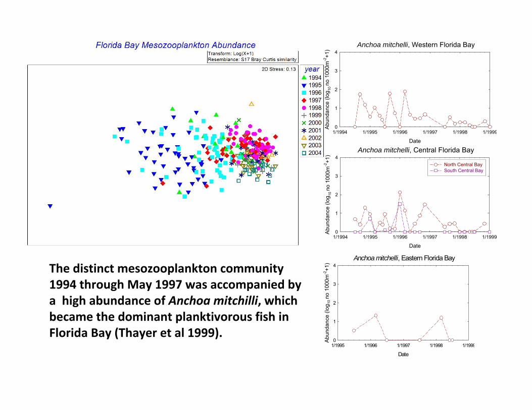
Canonical Correspondence Analysis of water quality (FIU) and sponge community distribution (ODU/FMRI) data at sites throughout the region reveal three sponge groups with similar water quality requirements or tolerances.

• Group 1: low TP, DO, TEMP, and TURB and high variability in all N measures

• Group 2: low levels of DIN, TON, and TOC and high variability in P and ChlA

• Group 3: high Nox, high salinity and highly variable salinity and DO

Water Quality - Sponge Distribution Association

Butler & Weisz unpub.

Summary of 2007 Bloom Effects on Sponges

• Impact of blooms on hard-bottom communities appears to be similar to that in 1991-1992, although bloom genesis different

• Sponge die-off widespread in middle Florida Keys (200 km2 area) and full recovery will take decades if no further blooms

• Sponge tolerance may be related to species-specific difference in filtration efficiencies

• Ecosystem filtration capacity and habitat structure is greatly diminished in impacted areas, with cascading effects on juvenilelobster abundance and aggregation with possible effects on theirpredator-prey and disease dynamics

Butler & Behringer unpubl.

Sponge & Octocoral Salinity Tolerance Experiments:

•All sponges tested survived sub-optimal salinities better in winter than summer; the reverse was true of octocorals.

•Sponge & Octocoral survival was similar whether exposed to low salinity for a few days or a few weeks (i.e., press vs. pulse experiments).

0

25

50

75

100

C. alloclada H. lachne I. campana I. variabilis S. vesparium

15 ppt 25 ppt 30 ppt 35 ppt

% S

urv

ived

Species

0

25

50

75

100

C. alloclada H. lachne I. campana I. variabilis S. vesparium

15 ppt 25 ppt 35 ppt 45 ppt

% S

urv

ived

Species

Butler unpubl. data

Angular Sea WhipPurple Sea Plume

n = 6 - 16 per treatment

15 20 453525

NoneSurvived

Salinity (psu)

20

40

60

80

100

0

Perc

ent S

urvi

val

n = 8 per treatment

15 20 4535

NoneSurvived

25

NoneSurvived

NoneSurvived NA

Salinity (psu)

Spongessummer

winter

Octocorals

summer winter

Behringer & Butler 2006 Oecologia

Stable isotope analysis of representative benthic macrofauna from hard-bottom habitat in Florida Bay suggests that:• algae, not seagrass, is the major source of primary productivity for hard-bottom higher trophic webs (sponge, mollusc, echinoderm, lobster)

• effect of plankton blooms on trophic structure not evident ~ 5 yrs later

Viral Transmission: Laboratory Trials• Inoculation: 95% transmission in 80d

• Ingestion: 42% transmission in 80 d

• Waterborne: 10 – 50% transmission in 80d;effectiveness declines with lobster size & distance

No transmission tosympatric decapodsvia inoculation

Spotted SpinyLobster

Spider Crab Stone Crab

• Contact: 11 – 63% transmission in 80d;transmission decreases withsize

Contact Transmission

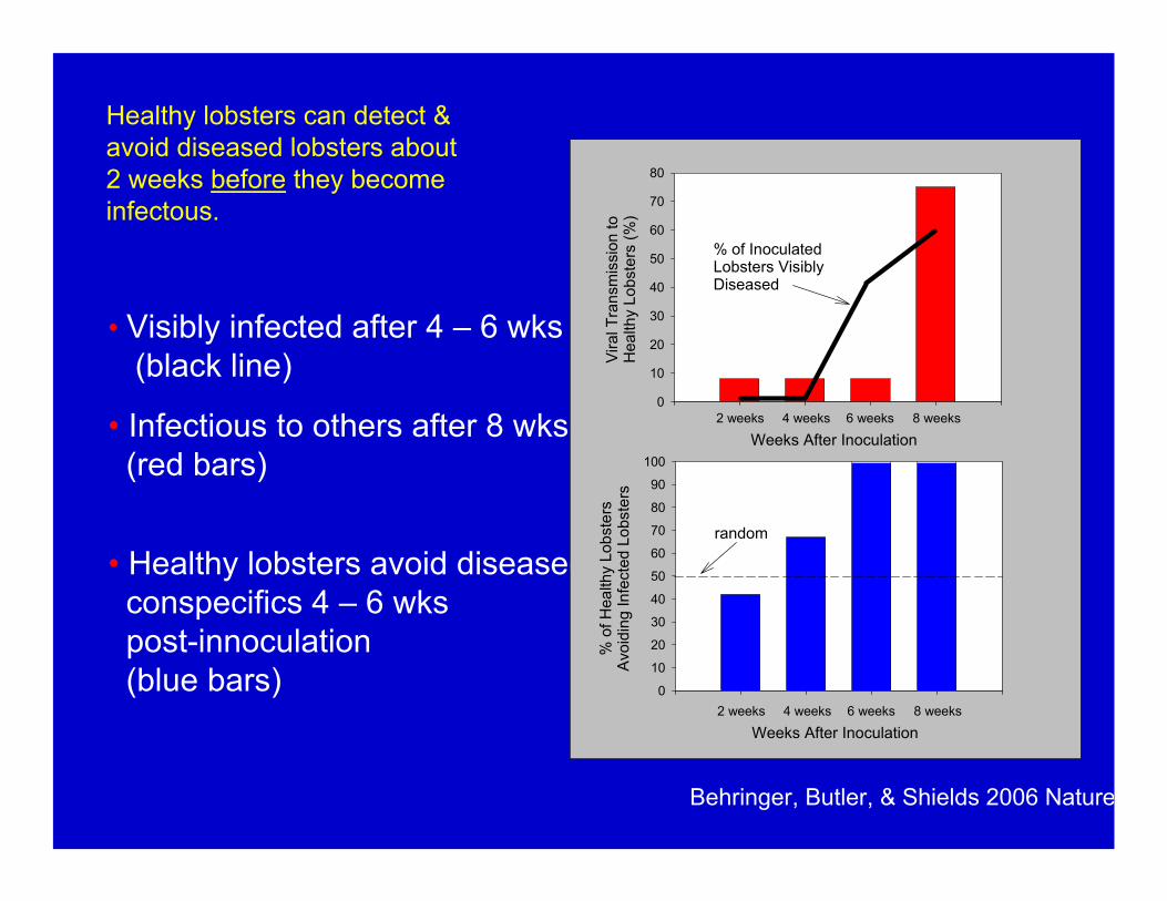
Healthy lobsters can detect &avoid diseased lobsters about2 weeks before they becomeinfectous.

• Visibly infected after 4 – 6 wks (black line)

• Infectious to others after 8 wks (red bars)

• Healthy lobsters avoid diseased conspecifics 4 – 6 wkspost-innoculation (blue bars)

Vira

l Tra

nsm

issi

on to

H

ealth

y Lo

bste

rs (%

)

0

10

20

30

40

50

60

70

80

2 weeks 4 weeks 6 weeks 8 weeks

Weeks After Inoculation

% of InoculatedLobsters Visibly Diseased

% o

f Hea

lthy

Lobs

ters

A

void

ing

Infe

cted

Lob

ster

s

0

10

20

30

40

50

60

70

80

90

100

2 weeks 4 weeks 6 weeks 8 weeks

Weeks After Inoculation

random

Behringer, Butler, & Shields 2006 Nature

(Paris, Butler, Cowen, unpubl.data)

Lobster Caribbean matrix spawning: June 2004

Where do Florida’s Lobster Come From and Go To?

• Simulations using a coupled bio-physical oceanographic model developed for reef fish (modified for lobster to include larval behavior & PLD) are less surprising for Florida than elsewhere in Caribbean and suggest:

• Florida’s lobster recruits come from all over the Caribbean …

… whereas the larvae spawned by lobsters in Florida are lost from the system

Fish and Invertebrate Assessment Network (FIAN)

Michael B. RobbleeJoan A. Browder

CERP-RECOVER-MAP

Region-wide Pink Shrimp Density, by MAP Collection

Fish and Invertebrate Monitoring Network (FIAN)

Pink Shrimp Abundance Metrics Over Time in Johnson Key Basin

Fall Pink Shrimp Density vs. Salinity in Johnson Key Basin

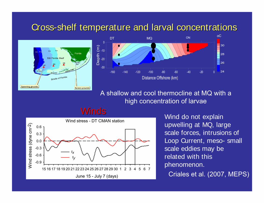
CrossCross--shelf temperature and larval concentrationsshelf temperature and larval concentrations

-160 -140 -120 -100 -80 -60 -40 -20 0

Distance Offshore (km)

-30

-20

-10

0

De

pth

(m

)

24

26

28

30

oCDT ONMQ

WindsWindsWind do not explain upwelling at MQ, large scale forces, intrusions of Loop Current, meso- small scale eddies may be related with this phenomenon.

Wind stress - DT CMAN station

June 15 - July 7 (days)

15 16 17 18 19 20 21 22 23 24 25 26 27 28 29 30 1 2 3 4 5 6 7Win

d st

ress

(dyn

e cm

-2)

-0.9

-0.6

-0.3

0.0

0.3

0.6

tx ty

Criales et al. (2007, MEPS)

A shallow and cool thermocline at MQ with a high concentration of larvae

Linear internal tides (LIT)A shallow thermocline with strong density

gradients and high frequency motions of ~ 12 h

Strong vertical shear, vertical turbulent mixing

High concentration of larvae at the shallow thermocline

LIT don’t contribute to onshore transport but convergent current may concentrate larvae at the upper layer

From 17:30h to 15:30h

Temperature

-20

-18

-16

-14

-12

-10

-8

-6

-4

-2

Dept

h (

m)

From 17:30h to 15:30h

Salinity

-20

-18

-16

-14

-12

-10

-8

-6

-4

-2

From 17:30hto 15:30h

Density

-20

-18

-16

-14

-12

-10

-8

-6

-4

-2

Marquesas, July 3-4, 2004

Temperature, salinity Temperature, salinity and density and density

C urren t shear (10 -4 s -2 )

0 10 20 30 40

(du /dz)2

(dv/dz)2

R ichardson num bers0.0 0 .5 1 .0 1 .5 2 .0

D ens ity grad ient (kg m -3)-0 .2-0 .10 .0

Dep

th (m

)

0

5

10

15

20

Density, shear and Richardson numbersDensity, shear and Richardson numbers

Cur

spd

(cm

s-1

)

-60

-30

0

30

60

0

40

80

120

0

100

200

300

0

40

80

120

160

Protozoeae Myses Postlarvae

17192123 1 3 5 7 9 111315

Larv

al fl

ux(l

* 100

m-2

s-1

)

-6

-3

0

3

6

July 3-4, 2004 (h)

17192123 1 3 5 7 9 111315 17192123 1 3 5 7 9 111315

(+) onshore

(-) offshore

Larval fluxes and onshore transport

Dep

th (m

)

-12

-8

-4

0

WMD

Evidence of a Flood Tidal Transport (FTT) a type of STSTfor myses and postlarvae at ~ 80 km from nursery grounds

Investigation of Factors Influencing the Distribution of Clown and Code Gobies

• The hypothesis was that M. gulosus would be more tolerant to salinity shifts than G. robustum.

• M. gulosus inhabits northeastern Florida Bay where salinity is more variable than in the habitat over which G. robustum is distributed.

• To test this hypothesis, acute (e.g., “plunge-type”) salinity tolerance tests were performed with both species.

• Both species were remarkably tolerant to rapid shifts in salinity, and there was no compelling evidence for differences in acute salinity tolerance.

Clown goby occurs more in seagrass than sand in absence of code goby, but more in sand than seagrass in presence of code goby.

Code goby occurs more in seagrass than in sand whether or not clown goby is present.

Clown goby

Code goby

Evidence for species interactions and dominance:

Code goby is the dominant species.

Juvenile Spotted Seatrout Monitoring Areas

Chris Kelble, Allyn Powell, Joan Browder

Juvenile spotted Seatrout, Cynoscion nebulosus, density and frequency of occurrence vary interannually and geographically

Frequency of occurrence is inversely related to salinity in 3 of the 4 sub-regions, indicating susceptibility to changes in hydrology.

Temperature bins (C)

Trou

t den

sity

<26.0 26.0-28.7 28.7-30.5 >30.50.00.51.01.52.02.5

estimate+/- 2 S.E.

Salinity bins (ppt)

Trou

t den

sity

<33.0 33.0-36.4 36.4-39.5 >39.50.00.51.01.52.02.5

Seagrass biomass bins (dry g/m^2)

Trou

t den

sity

<17.9 17.9-45.8 45.8-93.9 >93.90.00.51.01.52.02.5

Based on AIC, the best GLM for predicting seatrout density included all three explanatory variables (water temperature, salinity, and seagrass biomass). Estimated seatrout density increased with greater temperature, decreased with greater salinity, and increased but saturated with greater seagrass biomass.

Fish-Habitat Suitability usingGeneralized Linear Models

Example: Spotted Seatrout (Cynoscion nebulosus)General Model

Fish Abundance = f (Habitat Variables)Data

Source: FWC fishery-independent surveys

Location: Charlotte Harbor

Time Period: 1989-2000

Season: Late summer through fall

Sampling Effort: n=106 to 307 each year-season

Key Biological Data: Catch-per-unit-effort (CPUE) and length composition

Key Environmental Data: Depth, bottom type, salinity, temperature

Target Seatrout Lifestage: Early juvenile (age 1-4 months, length 15-80 mm

Key Processing Step: CPUE data inter-calibrated among different samplinggears (seines, trawls, dropnets, etc.)

Jerald S. Ault, Steven G. Smith & William B. Perry

Two-Stage Model Fitting Procedure

Two-Stage Generalized Linear Model (GLM) Development1) Develop single habitat variable functions, e.g.,

p = f (depth) or u= f ( salinity)

Rationale: Two-stage estimation necessary due to high frequency of zerocatches common in fishery-independent survey data

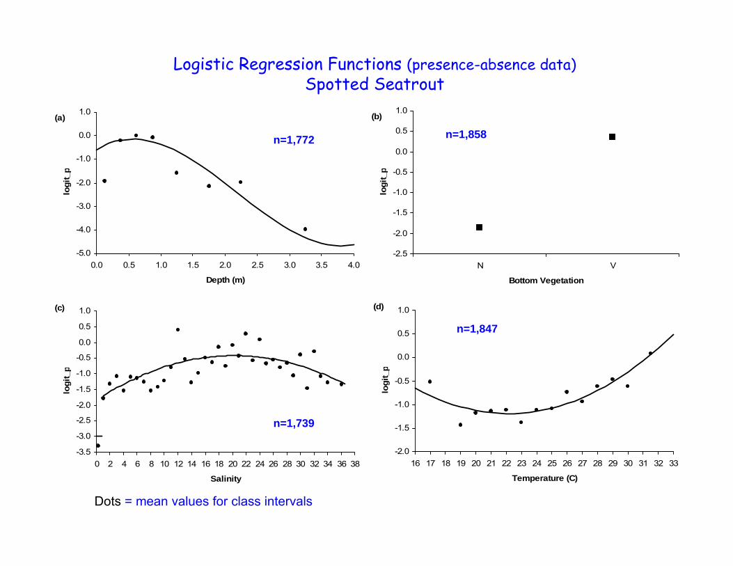
Stage 1: Logistic regression model using presence-absence data (p),p = f (habitat variables)

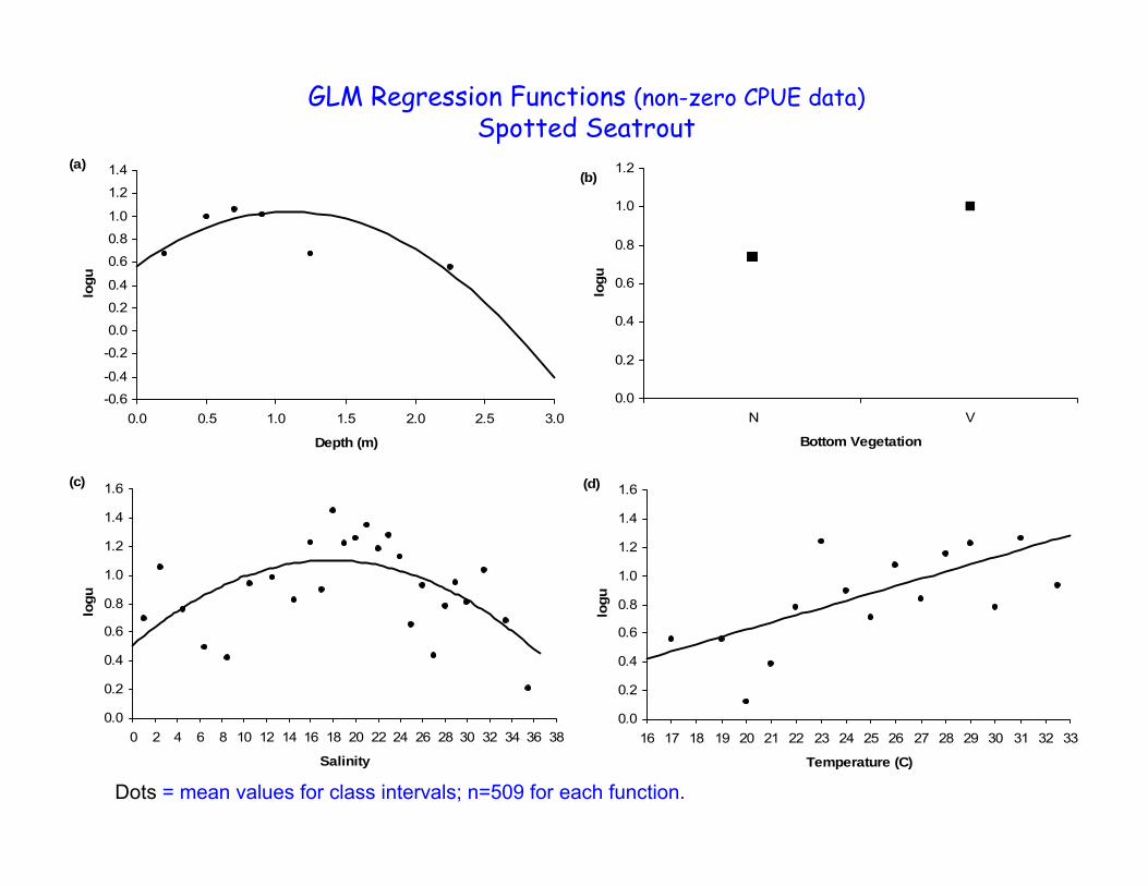
Stage 2: Generalized linear regression model using non-zero CPUE data (u),u = f (habitat variables)

Overall Prediction Model: CPUE = p x u

-5.0

-4.0

-3.0

-2.0

-1.0

0.0

1.0

0.0 0.5 1.0 1.5 2.0 2.5 3.0 3.5 4.0

Depth (m)

logi

t_p

(a)

-2.5

-2.0

-1.5

-1.0

-0.5

0.0

0.5

1.0

N V

Bottom Vegetation

logi

t_p

(b)

-3.5

-3.0

-2.5

-2.0

-1.5

-1.0

-0.5

0.0

0.5

1.0

0 2 4 6 8 10 12 14 16 18 20 22 24 26 28 30 32 34 36 38

Salinity

logi

t_p

(c)

-2.0

-1.5

-1.0

-0.5

0.0

0.5

1.0

16 17 18 19 20 21 22 23 24 25 26 27 28 29 30 31 32 33

Temperature (C)

logi

t_p

(d)

Logistic Regression Functions (presence-absence data)Spotted Seatrout

Dots = mean values for class intervals

n=1,739

n=1,772 n=1,858

n=1,847

-0.6

-0.4

-0.2

0.0

0.2

0.4

0.6

0.8

1.0

1.2

1.4

0.0 0.5 1.0 1.5 2.0 2.5 3.0

Depth (m)

logu

(a)

0.0

0.2

0.4

0.6

0.8

1.0

1.2

N V

Bottom Vegetation

logu

(b)

0.0

0.2

0.4

0.6

0.8

1.0

1.2

1.4

1.6

0 2 4 6 8 10 12 14 16 18 20 22 24 26 28 30 32 34 36 38

Salinity

logu

(c)

0.0

0.2

0.4

0.6

0.8

1.0

1.2

1.4

1.6

16 17 18 19 20 21 22 23 24 25 26 27 28 29 30 31 32 33

Temperature (C)

logu

(d)

GLM Regression Functions (non-zero CPUE data)Spotted Seatrout

Dots = mean values for class intervals; n=509 for each function.

Model Development (cont.)2) Combine single variable functions into multiple variable functions:

p = f (depth, bottom type, salinity, temperature) for logistic regression and

u= f ( depth, bottom type, salinity, temperature) for GLM regression

Florida Bay CPUE MappingUse fish-habitat regression models to predict CPUE for each 200 x 200 m

grid cell of the digital composite habitat map

Mud Banks

ModelGrid

200 x 200 m

ENP Boundary

Seagrass

Hardbottom

No Vegetation

Florida Bay Benthic Habitats

Rsmas_grid_g.shp-1.332 - -1.056

-1.056 - -0.952

-0.952 - -0.862

-0.862 - -0.789

-0.789 - -0.724

-0.724 - -0.659

-0.659 - -0.592

-0.592 - -0.527

-0.527 - -0.464

-0.464 - -0.4

-0.4 - -0.315

-0.315 - -0.207

-0.207 - -0.083

-0.083 - 0.017

FloridaBay

Florida Bay Bathymetry

Hsm_resp.shp0

0

0.001 - 1

1.001 - 20

20.001 - 33.29

33.3 - 33.8

33.8 - 34.3

34.3 - 35.2

35.2 - 35.7

35.7 - 36.1

36.1 - 36.6

36.6 - 37.2

37.2 - 37.3

37.3 - 37.7

37.7 - 37.8

37.8 - 38

38 - 38.1

38.1 - 38.3

38.3 - 38.4

38.4 - 38.6

38.6 - 38.8

38.8 - 39.1

39.1 - 39.2

39.2 - 40.7

40.7 - 40.8

40.8 - 41.7

41.7 - 41.8

41.8 - 41.9

41.9 - 42.2

42.2 - 43.2

43.2 - 45.7

45.7 - 45.8

45.8 - 46.5

46.5 - 50

50 - 53.1

53.1 - 54.5

54.5 - 62.7

62.7 - 72.1

72.1 - 72.8

FATHOM – Salinity April 2001

Hsm_resp.shp0

0

0.001 - 1

1.001 - 20

20.001 - 33.299

33.3 - 33.8

33.8 - 34.3

34.3 - 35.2

35.2 - 35.7

35.7 - 36.1

36.1 - 36.6

36.6 - 37.2

37.2 - 37.3

37.3 - 37.7

37.7 - 37.8

37.8 - 38

38 - 38.1

38.1 - 38.3

38.3 - 38.4

38.4 - 38.6

38.6 - 38.8

38.8 - 39.1

39.1 - 39.2

39.2 - 40.7

40.7 - 40.8

40.8 - 41.7

41.7 - 41.8

41.8 - 41.9

41.9 - 42.2

42.2 - 43.2

43.2 - 45.7

45.7 - 45.8

45.8 - 46.5

46.5 - 50

50 - 53.1

53.1 - 54.5

54.5 - 62.7

62.7 - 72.1

72.1 - 72.8

72.8 - 79.6

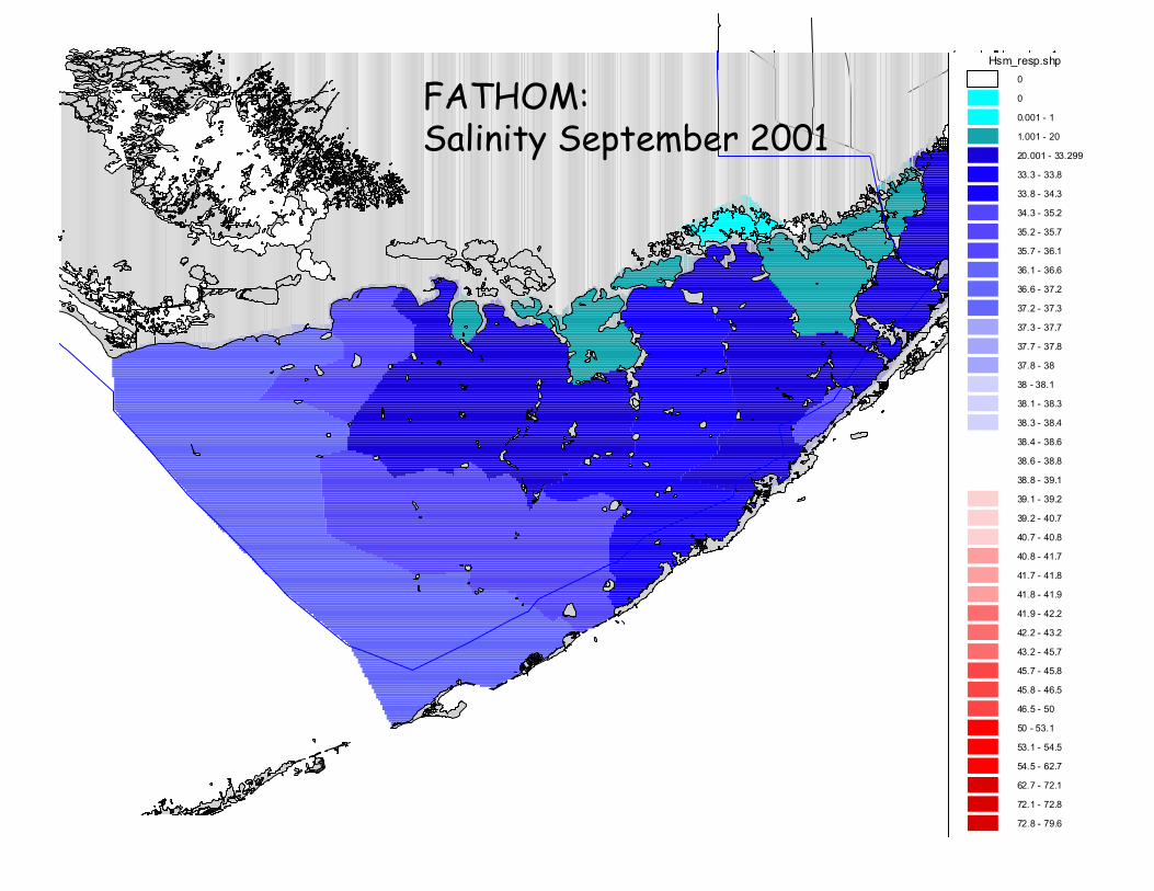
FATHOM:Salinity September 2001

Hsm_resp.shp0

0

0.001 - 1

1.001 - 20

20.001 - 33.299

33.3 - 33.8

33.8 - 34.3

34.3 - 35.2

35.2 - 35.7

35.7 - 36.1

36.1 - 36.6

36.6 - 37.2

37.2 - 37.3

37.3 - 37.7

37.7 - 37.8

37.8 - 38

38 - 38.1

38.1 - 38.3

38.3 - 38.4

38.4 - 38.6

38.6 - 38.8

38.8 - 39.1

39.1 - 39.2

39.2 - 40.7

40.7 - 40.8

40.8 - 41.7

41.7 - 41.8

41.8 - 41.9

41.9 - 42.2

42.2 - 43.2

43.2 - 45.7

45.7 - 45.8

45.8 - 46.5

46.5 - 50

50 - 53.1

53.1 - 54.5

54.5 - 62.7

62.7 - 72.1

72.1 - 72.8

72.8 - 79.6

FATHOM – Salinity June 2001

Hsm_resp.shp0 - 0.05

0.05 - 0.1

0.1 - 0.15

0.15 - 0.2

0.2 - 0.25

0.25 - 0.3

0.3 - 0.35

0.35 - 0.4

0.4 - 0.45

0.45 - 0.5

0.5 - 0.55

, 0.6

0.6 - 0.65

0.65 - 0.7

0.7 - 0.75

0.75 - 0.8

0.8 - 0.85

0.85 - 0.9

0.9 - 0.95

0.95 - 1

FloridaBay

Predicted Florida Bay Habitat SuitabilityJuvenile Seatrout -- June 2001

Hsm_resp.shp0 - 0.05

0.05 - 0.1

0.1 - 0.15

0.15 - 0.2

0.2 - 0.25

0.25 - 0.3

0.3 - 0.35

0.35 - 0.4

0.4 - 0.45

0.45 - 0.5

0.5 - 0.55

, 0.6

0.6 - 0.65

0.65 - 0.7

0.7 - 0.75

0.75 - 0.8

0.8 - 0.85

0.85 - 0.9

0.9 - 0.95

0.95 - 1

FloridaBay

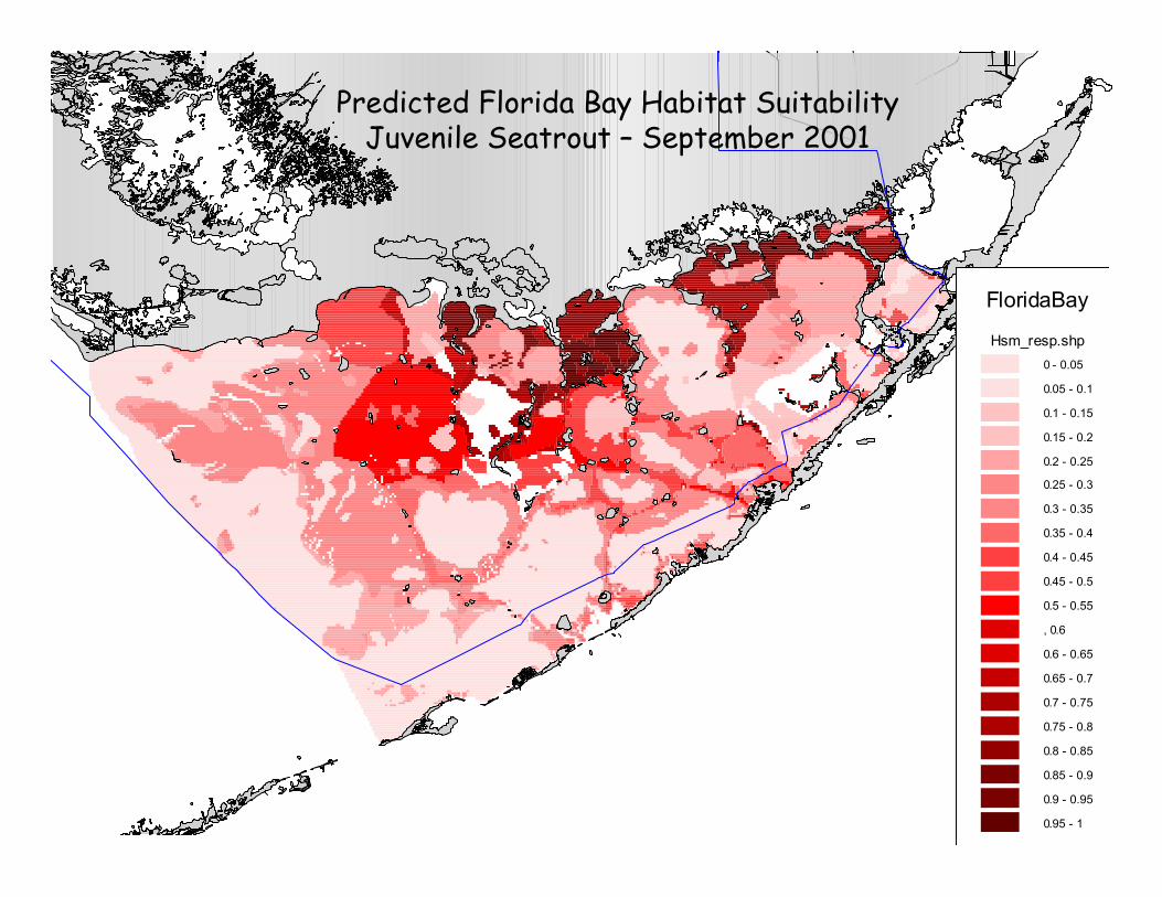
Predicted Florida Bay Habitat SuitabilityJuvenile Seatrout – September 2001

Effects of Hurricane-Induced Fragmentation of Mangrove Forest on

Habitat and Fish

Carole C. McIvor1, Noah Silverman,1,2

and Victor Levesque3

1 USGS, FISC, St Petersburg, FL2 ETI Professionals, Tampa FL3 USGS, FISC, Tampa, FL

Funding: USGS Global Climate Change, USGS Priority Ecosystem Science

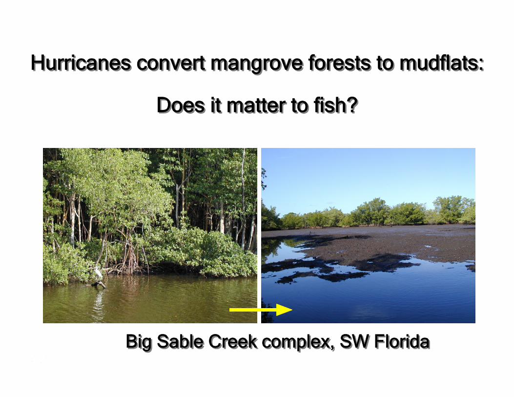
Hurricanes convert mangrove forests to mudflats:

Does it matter to fish?

Hurricanes convert mangrove forests to mudflats:

Does it matter to fish?

Big Sable Creek complex, SW FloridaBig Sable Creek complex, SW Florida

Nek

ton

(indi

vidu

als)

100

m-3

of w

ater

Mangrove Mudflat

Wet

Dry

Per volume of water, mangrove forests contain higher numbers and greater biomass of fish than do mudflatsn

u

ConclusionsHurricane-Driven Fragmentation of Mangroves

Found

• Water-column fish replaced benthic fish on mudflats

• Decreased fish density, biomass

Given

• Rising sea level

• Probable increased hurricane intensity

Expect

• Increased forest fragmentation at landfall

• Decreasing fisheries productivity at impact site

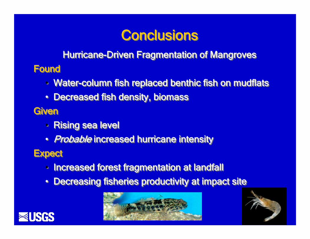
ConclusionsHurricane-Driven Fragmentation of Mangroves

Found

• Water-column fish replaced benthic fish on mudflats

• Decreased fish density, biomass

Given

• Rising sea level

• Probable increased hurricane intensity

Expect

• Increased forest fragmentation at landfall

• Decreasing fisheries productivity at impact site

OverviewContinuing and new research is sharpening our understanding of the processes that shape the ecology of Florida Bay and the influence of salinity on the distribution and abundance of faunal indicators—essential to CERP.Specific thresholds, preferences, or optima for individual species that can be directly used in evaluation of alternative CERP scenarios:

SpongesLittle fishes (Rand and Bachmann ) -- the FIU salinity tolerance experiments But rainwater killifish still neededMore trials at upper limits of salinity needed

Future work should focus especially on acquiring and improving specific information about the relationship of species and communities to salinity, as well as other potential influencing factors (e.g., nutrients, turbidity) on faunal species and communities that may be changed by CERP. Basic ecological studies such those on hardbottom habitat are needed for other important habitats of Florida Bay.More research and monitoring attention should be given to the lower southwest Florida coast:

Whitewater Bay to Lostmans RiverChokoloskee BayPicayune Strannd (Fakahatchee, Faka Union, and Pumpkin)

Acknowledgments and Apologies

I would particularly like to thank Savanna Howington of Everglades National Park for sharing information and materials from the National Park Service CESI Program. I also thank the many investigators who provided slides to illustrate discussion of their work. I apologize for any inadvertent slips in interpretation of their work. I also apologize for any omissions.