research papers

568 doi:10.1107/S1600577514001416 J. Synchrotron Rad. (2014). 21, 568–579

Journal of

SynchrotronRadiation

ISSN 1600-5775

Received 24 April 2013

Accepted 17 February 2014

# 2014 International Union of Crystallography

Unsupervised cell identification onmultidimensional X-ray fluorescence datasets

Siwei Wang,a* Jesse Ward,b Sven Leyffer,a Stefan M. Wild,a Chris Jacobsenb,c,d and

Stefan Vogtb

aMathematics and Computer Science Division, Argonne National Laboratory, 9700 South Cass

Avenue, Argonne, IL 60439, USA, bAdvanced Photon Source, Argonne National Laboratory,

9700 South Cass Avenue, Argonne, IL 60439, USA, cDepartment of Physics and Astronomy,

Northwestern University, 2145 Sheridan Road, Evanston, IL 60208, USA, and dChemistry of Life

Processes Institute, Northwestern University, 2170 Campus Drive, Evanston, IL 60208, USA.

*E-mail: siweiw@gmail.com

A novel approach to locate, identify and refine positions and whole areas of cell

structures based on elemental contents measured by X-ray fluorescence

microscopy is introduced. It is shown that, by initializing with only a handful

of prototypical cell regions, this approach can obtain consistent identification

of whole cells, even when cells are overlapping, without training by explicit

annotation. It is robust both to different measurements on the same sample and

to different initializations. This effort provides a versatile framework to identify

targeted cellular structures from datasets too complex for manual analysis, like

most X-ray fluorescence microscopy data. Possible future extensions are also

discussed.

Keywords: X-ray fluorescence microscopy (XFM); unsupervised object recognition;cell identification; trace element distributions; modeling overlapping cells.

1. Introduction

X-ray fluorescence microscopy (XFM) provides submicro-

meter-resolution information on the localization and quantity

of all but the lightest elements. For studies of micrometer-thick

biological specimens, it provides this information with lowest

dose for a given elemental sensitivity (Kirz, 1980), so that it

has emerged as a powerful method for studies in biology and

medicine (Paunesku et al., 2006). By using high-resolution

optics such as Fresnel zone plates, multi-keV X-rays are

focused to a small spot through which the specimen is scanned.

Absorption of these X-rays leads to the ejection of core shell

electrons, and photons at characteristic elemental fluorescence

energies are emitted as outer-shell electrons fill the core shell

vacancies. A competing process of emission of Auger electrons

reduces the fluorescence yield (i.e. the efficiency of conversion

of electron holes to characteristic X-ray fluorescence, in

particular for the lighter elements). Even then, X-ray fluor-

escence detection is still the preferred mode of contrast for

elemental mapping because the escape depth of Auger elec-

trons from the sample is extremely limited (Tan et al., 1982).

An energy-dispersive detector is used to record the energy

of individual X-ray fluorescence photons, thus providing

information on elemental content at that pixel location. These

multispectral data typically contain 1000 or more energy

channels per pixel, which in our case have been analyzed to

obtain concentrations of chemical elements as described in x3.

We are not the first to recognize that scientific capability for

intuitive understanding is being overwhelmed by the volume

and complexity of data generated in modern microscopies.

In light microscopy, Swedlow et al. (2009) have noted that

‘multidimensional imaging has driven a revolution in modern

biology, yet the significant data management and analysis

challenges presented by these new complex datasets remain

largely unsolved’. In recognition of these challenges, we have

already made some progress. Members of our team have

written a program called MAPS (Vogt, 2003) for quantifica-

tion and fitting of multidimensional X-ray fluorescence images

and a cluster-analysis-based program PCA_GUI for classifi-

cation and analysis in soft X-ray spectromicroscopy (Lerotic et

al., 2004, 2005) (this program has migrated to an open-source

project at http://code.google.com/p/spectromicroscopy).

MAPS carries out the analysis required to go from per-pixel

fluorescence spectra to per-pixel elemental concentration,

along with analysis through the manual generation of spatial

regions of interest; enhancements to include principal

component analysis and clustering are promising but not yet

reliable enough for unsupervised analysis of large datasets.

PCA_GUI provides cluster analysis but suffers from negative

unphysical weightings in some analyses (now being addressed

through the use of non-negative matrix factorization). Other

software packages have also been developed to analyze X-ray

fluorescence datasets, for example PyMCA (Sole et al., 2007)

as well as GeoPIXE (Ryan et al., 2002). Each of these

packages tends to have specific areas they are optimized for;

but, overall, these efforts do not yet appear to be as advanced

as clustering and machine-learning analysis implemented in

optical microscopy (Ljosa & Carpenter, 2009) or hyperspec-

tral analysis used in aircraft and satellite imaging (Plaza et al.,

2004). Our goal here is to provide object recognition directly

from X-ray fluorescence spectra with no subsequent higher-

level processing required, so as to greatly enhance how we

approach and understand the rich data sets generated from

X-ray fluorescence excitation in electron, proton and X-ray

excitation microscopy methods.

Based on optical microscopy, magnetic resonance imaging

and other medical imaging modalities, many object recogni-

tion methods are proposed to automatically (Wolz et al., 2010;

Arteta et al., 2012; Cortes & Amit, 2008) or semi-automatically

(Aydin et al., 2010; McCullough et al., 2008; Lin et al., 2003)

identify cellular structures. However, cell identification using

XFM has unique challenges. Firstly, it requires modeling a

large number of chemical elements simultaneously. Most of

the methods focused on optical microscopy can only deal with

one or several independent intensity channels. Secondly, there

is no known manual annotation dataset to serve as a large-

scale training example, hence most supervised learning

approaches [support vector machines (Kasson et al., 2005; Tao

et al., 2007; Wang et al., 2007), Markovian random fields, min-

max flow graph cut (Wolz et al., 2010; Yin et al., 2010), Potts

model (Russell et al., 2007)] are not applicable. Thirdly,

modeling overlapping cellular structures in XFM datasets is

more challenging compared with that in other related imaging

problems; an XFM dataset provides pixel-level localization

and quantity of elements. Therefore, it is necessary to model

how different cells overlap with each other. Nevertheless, most

known methods do not model cell overlap explicitly; instead

they either generate nonoverlapping regions from overlapping

cells (Arteta et al., 2012; Lin et al., 2003) or only process cells

at most touching at their boundaries (Bergeest & Rohr, 2011,

2012). In x7, we will discuss the difference between our

method and a representative cell counting routine (‘analyze

particle’ from ImageJ) in more detail.

We propose here a novel unsupervised cell identification

approach to tackle these unique challenges of XFM datasets.

Without manual annotations, our approach can locate, identify

and refine positions and areas of cellular structures (including

overlapping cells) based on their elemental content from a

large number of elements simultaneously.

To demonstrate this approach, we apply it to a dataset of

three intermixed cell types. We begin by using MAPS to

reduce the acquired fluorescence spectra into quantitative

concentrations of nine chemical elements. As input para-

meters for subsequent analysis, the approach accepts lower

bounds of cell sizes, averages and standard deviations of cell

contents from a few hand-drawn regions of interest (ROIs) for

each type. (These hand-drawn ROIs can in the future be

replaced by representative contents from other reference data

or learned automatically.) Then we use a generalized like-

lihood ratio test to model the configuration of multiple over-

lapping cells. Afterward, we apply two procedures [boundary

delineation (x4.3) and pixel refinement (x4.4)] to further

improve the boundaries of identified cells.

The paper is organized as follows. In x2, we provide a high-

level description of the components of our problem and

approach. In x3, we discuss sample preparation, data acquisi-

tion and the datasets we employed in evaluating the consis-

tency and robustness of this approach. We will also provide

specific assumptions for our test dataset with respect to our

general assumptions in x2. In x4, we introduce the four

underlying procedures in detail: preprocessing, estimating

group configuration, boundary delineation and pixel refine-

ment. Currently, each procedure can be viewed as solving an

optimization problem, the solution of which is then passed

as an input to the next procedure. However, this approach can

be modified such that the output of the last step can serve as

the input to the first step. We report our results in x5 and

demonstrate that this approach generates robust statistics of

cell populations with respect to initial parameters in x6. Since

this cell identification approach is in early stages of develop-

ment, many opportunities for improvement remain, and we

will discuss some of them in x7.

2. Problem and overview

We address the fundamental question: ‘Where are the (whole)

cells?’ based on recorded elemental content in an XFM

dataset. The goal of our approach is to identify cells of

different types, while also allowing for multiple cells to

overlap. We give a broad overview of our approach here,

which is described in detail in x4.

A key difficulty here is that often no manual annotation is

available to serve as a reference; we only know both the total

elemental contents of the whole cell areas and shape, and size

of cells of a given type can be employed as salient features. We

use the following two classes of expert-informed cell features

to initialize this approach:

(i) Morphology. We assume that all cells of a specific type

have somewhat similar sizes and shapes.

(ii) Content. We assume that cells of a specific type have

similar total content in their characteristic elements, and that

these characteristic elemental contents are distinct compared

with cells of other types.

The initial inputs for this approach are thus information on

the morphology and content features. Preprocessing of the

putative cells (x4.1) is done by image segmentation.

We first divide pixels of the image of a given characteristic

element into foreground and background components (i.e.

based on their intensity). We then partition all foreground

pixels into groups via the recursive min-cut algorithm (Dhillon

et al., 2007) and then fit a minimum-area ellipse around each

of these segments as the initial guess of cell areas. Here, we

deliberately initialize the partitioning algorithm so that we

oversegment (i.e. all actual cells are covered with at least one

group). We chose this algorithm because it is unsupervised

and oversegmentation is straightforward.

This oversegmentation conditions the configuration esti-

mation procedure in x4.2 to focus on evaluating group

research papers

J. Synchrotron Rad. (2014). 21, 568–579 Siwei Wang et al. � Unsupervised cell identification 569

configurations with potentially reduced number of cell groups.

This estimation procedure determines whether merging two

groups or deleting a group will represent the total content

better than the current configuration. We represent the total

content criteria with Gaussian distributions (specified by a

mean and diagonal covariance) obtained from the given

content inputs.

After we estimate the configuration of cell groups, we refine

these putative cell groups by adjusting their boundaries based

on a total elemental content criteria (see x4.3). This procedure

aims at recovering pixels that are within a cell but were

initially relegated to the background because of thresholding.

For every boundary we obtain by this procedure, we

compensate for potential smoothness discrepancies using a

pixel refinement procedure (see x4.4). This procedure ensures

that the resulting areas cover the group of pixels best for their

corresponding cells.

This multistep approach is versatile and can be applied to

a broad class of identification problems. The components

described here can also be employed independently or

combined to answer different scientific questions. An over-

view of this approach is presented in Procedure 1. Table 1 in

the supporting information illustrates all steps of this proce-

dure.1

Procedure 1. Overview of the approach.

Inputs: pixels P of an XFM dataset, cell types T , characteristic

element et and lower bound of size st for all t 2 T , means and

standard deviations of representative cell contents;

� Preprocessing;

for all t 2 T

Obtain foreground and background of et ;

Partition foreground pixels using elemental map of et , such

that all segments contain at most st pixels;

Obtain groups Gt of type t by using minimum-area ellipses

to cover all individual segments;

end for

� Estimation of group configuration: obtain groups GG from

initial groups G = [tGt by either merge or deletion;

� Optimization of group boundaries: delineate boundaries

of all groups g 2 GG using both morphology and content

features;

� Local pixel refinement: refine pixel boundaries of all

g 2 GG.

3. Sample and data

We deliberately chose a combination of very different cell

types to verify that the algorithm is able to work with this

diversity, and to make sure a human observer can easily test

the accuracy of the algorithm (differentiation between two

very similar subpopulations can be achieved by statistically

analyzing extracted elemental content resulting from our

algorithm). The specific cell types were chosen on the basis of

availability, use as model systems elsewhere in biology, and

expected differences in elemental content, cell size and

morphology. Red blood cells have a well known dumbbell

shape, and were expected to contain relatively more iron than

other cell types because of the presence of heme iron in

hemoglobin (Hawkins et al., 1954), and little else. By

comparison, yeast cells are expected to be smaller, and have

high Zn as well as P content (Marvin et al., 2012). As a third

cell type with a complementary elemental content we chose

the green algae Chlamydomonas with high manganese levels

because of the presence of manganese in photosystem II

(Dismukes, 1986).

Washed and pooled rabbit red blood cells (rbc) at 10%

hematocrit were purchased from Lampire Biological

Laboratories (Pipersville, PA, USA). A 1 ml volume sample

was drawn and centrifuged for 10 min at 600g. The super-

natant was discarded, and cells were resuspended in a solution

of 200 mM sucrose and 10 mM PIPES (Good et al., 1966), both

from Sigma-Aldrich (St Louis, MO, USA). Yeast cells were

inoculated in 2.5 ml of sterile YPD media (Lundblad & Struhl,

2001) and grown in a shaking incubator at 303 K and

300 r.p.m. for 24 h. A 1 ml volume sample was drawn and

centrifuged for 10 min at 600g. The supernatant was discarded,

and cells were resuspended in a solution of 200 mM sucrose

and 10 mM PIPES.

Algae cells were provided by Qiaoling Jin (Argonne). The

wild-type strain of Chlamydomonas reinhardtii was purchased

from ATCC (Manassas, VA, USA) and grown mixotrophically

in TAP medium (Gorman & Levine, 1965) on a rotary shaker

(120 r.p.m) at 298 K and in the presence of �100 mmol

photons m�2 s�1 of photosynthetically active light. A 1 ml

volume sample was drawn and centrifuged for 2 min at 600g.

The supernatant was discarded, and cells were resuspended

in a solution of 200 mM sucrose and 10 mM PIPES. Equal

volumes of red blood cells, yeast cells and algae cells were

suspended in 200 mM sucrose and 10 mM PIPES and then

mixed together. A 2 mL volume was spotted onto a 200 nm-

thick silicon nitride window (Silson Ltd, Northampton, UK)

and allowed to air dry overnight.

X-ray fluorescence imaging was performed at beamline 2-

ID-E at the Advanced Photon Source at Argonne, USA.

Undulator-produced X-rays at 10 keV incident energy were

focused to a spot size of 0.8 mm by 0.8 mm using Fresnel zone

plate optics (Xradia Inc., Pleasanton, CA, USA). Samples

were raster-scanned through the X-ray beam in fly-scanning

mode, covering about a (200 mm)2 area with a pixel size � =

0.3 mm in each direction, 666 � 667 pixels, and an effective

dwell time of 100 ms per pixel. Full fluorescence spectra were

detected at each pixel using a four-segment silicon drift

detector (Vortex-ME4, Hitachi High-Technologies Science

America, Northridge, CA, USA), with each detector segment

collecting a slightly different signal because of angular varia-

tions in scattered signals, different self-absorption paths to the

segment, and so on. These differences, resulting from the 15�

angle between the sample and the detector, are negligible for

high-Z elements, but can be significant for low-Z elements

(e.g. 50% for P).

research papers

570 Siwei Wang et al. � Unsupervised cell identification J. Synchrotron Rad. (2014). 21, 568–579

1 Supporting information for this paper is available from the IUCr electronicarchives (Reference: WA5055).

Every pixel in the XFM dataset originally contains the full

X-ray spectra recorded from the four detector segments.

These spectra were then processed by MAPS (Vogt, 2003),

which involves a fitting procedure and calibration based on a

standard with known elemental concentration to yield quan-

titative maps of elemental concentration in mg/cm2. Those

quantitative maps for the elements P, S, Cl, K, Ca, Mn, Fe and

Zn provided the input data for the analysis procedures

described here (Fig. 1).

Based on this specific information, we can derive the

following features for identifying cells in this test dataset:

(i) Morphology: all cells can be modeled as ellipses with

different sizes and shapes.

(ii) Content: all cells have consistent content in all nine

elements (P, S, Cl, K, Ca, Mn, Fe, Cu, Zn) resembling Gaussian

distributions. For each cell type, there is a characteristic

element which provides signature elemental content infor-

mation, i.e. Fe for red blood cells, Zn for yeast cells and Mn

for algae cells.

4. Detailed description of our approach

Here, we describe four individual components of Procedure 1

in detail. For a given image, we let P denote the set of pixels in

the image, with each pixel indexed by a pair of (column, row)

indices (x, y). We use uppercase roman letters to denote sets

of pixels and use calligraphic letters to refer to other types of

sets (e.g. index sets, elements, cell types) throughout the

sequel.

Let F and B denote disjoint sets of foreground and back-

ground pixels, respectively, so that P = F [ B. We designate a

group of pixels by Gg, where g 2 G denotes a group index.

Each group will have an associated type t 2 T ; in this paper

T = {algae, rbc, yeast}. Groups will ultimately be used to

define a cell, but we use the term ‘group’ to acknowledge that,

particularly in the initial steps of this approach, there may not

be a one-to-one correspondence between groups and cells.

The collection of all groups defines the foreground pixels as

F = [g2GGg. Associated with each group Gg will be a set of

local background pixels Bg, more formally defined in x4.1.2.

A region Rr (with r 2 R) consists of pixels belonging to one

or more groups and their local backgrounds. We let Gr � G

denote the set of groups belonging to region Rr so that Rr =

[g2GrðGg [ BgÞ. The sets Gr form a partitioning of G. We

denote the local background of region Rr by Br (defined in

x4.1.2).

In this paper, we limit the content computation to jEj = 9

elements, E = {P, S, K, Cl, Ca, Mn, Fe, Cu, Zn}. For a general set

of pixels Z, we define ceðZÞ to be the total content of Z in e

by summing over all pixels in Z using the elemental map for

element e 2 E. For example, for a single pixel Z = (x, y), we

use ceðx; yÞ to denote the content using the content map for

element e 2 E (see x3).

Using these notations, we organize our approach as follows:

(i) Preprocessing and image segmentation. Specify

elemental contents for each cell type, identify the foreground

pixels F, divide the foreground into jGj possibly overlapping

groups, and aggregate the groups into jRj disjoint regions

(x4.1). The putative groups serve as an initialization; they may

research papers

J. Synchrotron Rad. (2014). 21, 568–579 Siwei Wang et al. � Unsupervised cell identification 571

Figure 1Elemental maps for K, P, Mn, Fe and Zn, and visible-light micrograph of a mixture of three cell types (red blood cells, algae, yeast) used for subsequentanalysis. The quantified elemental content per pixel is shown in mg/cm2 in the intensity scale next to each map. The maps of particular elements obtainedby X-ray fluorescence microscopy hint at the characteristics of the different cell types: Mn is prevalent in algae and Fe in red blood cells, while Zn and Pare indicative of yeast cells. The visible-light micrograph was acquired at one focal plane and thus does not show all cells; slight distortions in relative cellpositions between the X-ray fluorescence maps and the visible-light micrograph are due to differences in viewing angles.

be deleted or merged to other groups in subsequent cell

identification procedures (see Fig. 4).

(ii) Estimation of group configuration. Given a set of groups

G and a set of disjoint regions R, adjust the number and areas

of groups of each type within each region to best match the

observed elemental contents (x4.2).

(iii) Optimization of group boundaries. Given putative cell

groups in each region, determine smooth curves to serve as

boundaries of the cells (x4.3).

(iv) Local pixel refinement. For the smooth boundaries in a

region that do not satisfy local optimality conditions, refine

each associated group so the content of its discrete set of

pixels best matches the content in a cell (x4.4).

To seed our preprocess procedure, we use per-hand iden-

tification of ROIs around a few isolated cells of each type. This

was appropriate for an initial study, though in the future the

seeding could be done from literature values for elemental

composition and area st.

In our case, the ROIs provide twofold information: (i) the

element or combination of elements provides characteristic

elemental maps that distinguish each specified cell type, and

(ii) the content from these ROIs is employed as representative

total elemental content of these cells. We use the former

information to preprocess the dataset and obtain initial

guesses for the areas of putative cells (x4.1.1). We use the

latter to refine these putative cells (x4.1.4).

4.1. Preprocessing and image segmentation

The first procedure is responsible for producing the repre-

sentative elemental distributions, a set of initial groups G and

regionsR, and the local backgrounds for each of these groups

and regions.

4.1.1. Initial group formation.. The input of the image

segmentation algorithm are the individual elemental maps

based on hand-drawn ROIs and the segment area bound st; for

purposes of oversegmentation, st is taken to be the smallest

cell area from the hand-selected ROI. The three cell types

have somewhat different sizes. We therefore set the st value of

each type t 2 T for subsequent analysis: we used st = 200

pixels (or 18 mm2) for red blood and algae cells, and st = 30

pixels (or 2.7 mm2) for yeast cells.

Using the individual elemental maps and segment area

bound st for all types in T , we then perform an image

segmentation using images from three characteristic elements

(Mn for algae, Fe for red blood cells and Zn for yeast). The

resulting segments (shown in Fig. 2) each locate a possible

area for a cell of type t.

Based on these segmentations, we form minimum-area

ellipses to cover pixels belonging to the same segment.

Ellipses are appropriate for the cell types considered here;

more complicated shapes can also be considered. The pixels

in each ellipse are used to define an initial group Gg. By

construction, all groups contain a contiguous set of pixels.

4.1.2. Region formation and background content. As

previously described, a region is defined as an area of groups

and their local backgrounds. Here, the local background Bg of

a group Gg is defined as a set of pixels within a distance � > 0

of the group,

Bg � fðx; yÞ 2 B : jx � xxj þ jy � yyj �

for some ðxx; yyÞ 2 Ggg; ð1Þ

where we recall that the foreground is defined as F = [g2GGg

and the background is defined as B = P \ F.

Therefore, a region Rr = [g2GrðGg [ BgÞ contains groups

that are either overlapping with each other or overlapping in

their local backgrounds. The local background of a region is

then defined in analogy to equation (1) as the background

outside of the region that is within a distance � of the region,

or

Br � fðx; yÞ 2 B \ Rr : jx � xxj þ jy � yyj �

for some ðxx; yyÞ 2 Rrg: ð2Þ

Although groups (as well as their backgrounds) may overlap,

the regions are disjoint. Thus a region provides a convenient

partitioning of the image into semi-independent structures,

while groups allow for the modeling of overlapping cells.

Initial groups, regions and local backgrounds for the entire test

dataset are illustrated in Fig. 3.

The primary purpose of obtaining local backgrounds is to

adaptively estimate the local background content. Knowledge

of the background content is important in XFM analysis.

When using energy-dispersive detectors to record the fluor-

escence signal, there will be some contribution at all energies

as a result of inelastic scattering and incomplete collection of

the charge deposited in the detector by fluorescence photons

(ideally this is resolved by the fitting procedure of MAPS as

described in x3). There may also be some signal as a result of

elements in the medium in which the cells where prepared.

The inhomogeneous background (see, for example, the K

channel in Fig. 1) in many of the elemental maps introduces

challenges for cell identification and for generating statistics

on elemental content of various cell types.

Analogous to total cell content introduced in x2, we also use

Gaussians to describe per-pixel local background content. For

research papers

572 Siwei Wang et al. � Unsupervised cell identification J. Synchrotron Rad. (2014). 21, 568–579

Figure 2Image segmentation result used to form the initial groups for yeast andred blood cells based on the markers Zn (a) and Fe (b), respectively.Algae cells are not shown because there are only five cells. All pixels ofthe same color belong to the same segment, hence they are treated as onesingle putative cell group in subsequent procedures.

example, �er denotes the mean (per-pixel) content of element

e in the local background of region Rr and is defined as

�er �1

jBrjceðBrÞ ¼

1

jBrj

Xðx;yÞ2Br

ceðx; yÞ: ð3Þ

We similarly define the sample variance in the local back-

ground Br,

�2er �

1

jBrj � 1

Xðx;yÞ2Br

ceðx; yÞ �1

jBrjceðBrÞ

� �2

: ð4Þ

4.1.3. Representative cell elemental content. For the

subsequent procedures we require statistics of the content of

each type of cell to broadly characterize the types of cells.

In the current approach, we represent the distribution of the

total elemental content in a cell as a truncated (imposing non-

negativity) Gaussian. Although other distributions can be

used in our framework, we focus on Gaussians here to illus-

trate the method based on a small number of distributional

parameters. In particular, if we assume that the contents for

cells of different types and elements are independent, we need

only to specify means and variances ð�et; �2etÞ for all e 2 E

and t 2 T .

If such information is unavailable, it can be estimated by

using a small number of expert hand-selected cells, particu-

larly those that are well separated from other cells in this

particular example. Given a collection G0ðtÞ of hand-selected

groups corresponding to cells of type t, we can use the sample

mean

��et ¼1

jG0ðtÞj

Xg2G 0ðtÞ

ceðGgÞ ð5Þ

and sample variance

�� 2et ¼

1

jG0ðtÞj � 1

Xg2G 0ðtÞ

ceðGgÞ � ��et

� �2ð6Þ

as estimates for �et and � 2et, respectively.

4.1.4. Content computation for groups. Here we describe

how to compute content for groups. Because we allow groups

to overlap, it is necessary to apportion the content given by an

elemental map among overlapping groups. A naıve way to

distribute the content ceðx; yÞ would be to split it equally

among the groups that contain the pixel ðx; yÞ. The approach

that we take is to account for the relative abundance of the

element with respect to the group’s type. Another way to

describe this is to split pixel content between groups which

contain that pixel weighted to the mean content per group and

type. For this we employ the representative means �et as

estimated in x4.1.3.

Formally, we let Gtðx; yÞ � G denote the set of groups of

type t 2 T that contain pixel ðx; yÞ. A single group of type t

containing ðx; yÞ is thus assigned the fraction of content

fetðx; yÞ ¼�etP

t 02T

Gt 0 ðx; yÞ�� ���et 0

: ð7Þ

By construction, the content from an elemental map is

preserved: summing over all groups containing ðx; yÞ yields

the elemental map content ceðx; yÞ. Taking into account the

background’s contribution and using this weighting, we define

the assigned content of element e 2 E for group g 2 G of type

t 2 T by

cegt ¼Pðx;yÞ2Gg

fetðx; yÞ ceðx; yÞ � �er

� �; ð8Þ

where r 2 R denotes the region that group Gg belongs to.

4.2. Estimation of group configuration

The image segmentation in x4.1 is used to provide an initial

group configuration (i.e. numbers and areas of groups).

However, two drawbacks prevent this configuration from

serving as putative cell areas: (i) only a single trace element for

each cell type is taken into account, whereas cells are usually

represented with multiple elements in XFM datasets; and (ii)

overlapping cells of the same type are not taken into account.

We now introduce an iterative procedure for adjusting this

initial group configuration to a more realistic configuration. In

each iteration, the current configuration is updated to better

match the region content with respect to the representative

cell contents (from x4.1.3). We use a generalized likelihood

ratio (GLR) test to determine whether such an update would

improve the configuration for region Rr. This GLR test is

formulated as (Wasserman, 2003)

max�0

LðH0jcrÞ

max�C

0

LðH 0jcrÞ: ð9Þ

The null hypothesis parameter space �0 = fH0g has the current

group configuration as its only hypothesis; the complementary

parameter space �C0 has alternative hypotheses with reduced

research papers

J. Synchrotron Rad. (2014). 21, 568–579 Siwei Wang et al. � Unsupervised cell identification 573

Figure 3(a) Illustration of groups (foreground pixels), regions and backgroundswith corresponding mathematical notations. The innermost solidboundaries represent the union of groups, the next boundaries (black,orange fill) represent the regions, and the outermost boundaries (pink)represent the union of regions and region backgrounds. (b) Overlayshowing distributions of Fe (red), Mn (green), Zn (blue) and the regionboundaries (white). Note that (a) illustrates a � = 2 pixel distance; we usea � = 5 pixel distance for both group and region background estimationin our experiments.

numbers of groups. We need only to consider alternative

hypotheses with fewer groups jG 0r j< jGrj (Wu & Nevatia, 2009)

because of the oversegmentation discussed in x4.1.

Even if we only reduce the number of groups, testing all

possible configurations is still prohibitive. To make this GLR

test computationally tractable, we limit the parameter space

�C0 to alternative hypotheses of exactly jGrj � 1 groups, either

through merging two groups g; g0 2 Gr (forming a new group

from Gg [Gg0) or deleting a group g 2 Gr .

The data here are the elemental content cr = ðcreÞ of all

pixels in region Rr. Assuming the contents of groups in a

region are independent, we can cast cr as the sum of the

contents [cg = ðcegtÞ] in the groups g 2 Gr and the contents

[cbr = ðcebrÞ] in the respective local backgrounds [g2GrBg.

Formally, for all e 2 E we have

cre ¼P

ðx;yÞ2fGg:g2Grg

ceðx; yÞ ¼ cebr þP

g2Gr

cegt; ð10Þ

where cegt is defined in equation (8). The likelihood of our null

hypothesis is thus evaluated as

LðH0jcrÞ ¼Q

g2Gr

LðH0jcgÞ

" #LðH0jcbrÞ: ð11Þ

The mean and variance of element e for group g (of type t) in

region Rr are defined by

~��egr ¼ �er Gg

�� ��þ ��et and ~�� 2egr ¼ �

2er Gg

�� ��þ �� 2et;

where ��et and �� 2et are defined in equations (5) and (6). The

likelihood L of group g is

LðH0jcgÞ ¼Ye2E

2� ~�� 2egr

!�1=2

exp �1

2

Xe2E

ðcegt � ~��egrÞ2

~��2egr

" #:

ð12Þ

The likelihood of the background is defined similarly, with the

background mean and variance of element e defined by

~��ebr ¼ �er

[g2Gr

Bg

���������� and ~��2

ebr ¼ �2er

[g2Gr

Bg

����������:

The likelihood of an alternative hypothesis H 0 is evaluated

similarly to the null hypothesis in equation (11). In the

merging and deleting operations, we now need only to modify

the appropriate terms corresponding to the configuration

differences between H0 and H0:

(i) Merging. If H 0 corresponds to merging adjacent groups

ðg; g0Þ, by convention the resulting group inherits the type t

from the first group g [we also consider the pair ðg0; gÞ]. The

new group has content computed by using the pixels Gg [Gg0

in equation (8). The updated means and variances for the new

group g00 are given by

~��eg00r ¼ �er Gg0 [Gg

�� ��þ ��et and ~�� 2eg00r ¼ �

2er Gg0 [Gg

�� ��þ �� 2et:

(ii) Deleting. If H 0 corresponds to deleting group g, then we

expand the background with all pixels only in group g. Those

pixels are

Gg � fðx; yÞ 2 Gg : 8g0 2 Gr \ fgg; ðx; yÞ =2 Gg0 g: ð13Þ

In the evaluation of joint likelihood, we drop the term with

respect to cg and update background means ~��eb0r and

variances ~�� 2eb0r as

~��eb0r ¼ �er

[g2Gr

Bg

[Gg

���������� and ~�� 2

eb0r ¼ �2

er

[g2Gr

Bg

[Gg

����������:

An example of how merging and deleting operations update

the group configuration in a region is shown in Fig. 4. The

outcome of this procedure (summarized in Procedure 2) is

a group configuration that better describes the elemental

content in every region.

Procedure 2. Estimation of group configurations (see x4.2).

Given regions R, groups G, elemental content cr, and mean

and variance of elemental content [e.g. from equations (5) and

(6)];

for all regions r 2 R do

repeat

Set NumRegChanged = 0;

Evaluate null hypothesis LðH0jcrÞ;

Find LðH0jcrÞ :¼ maxLðHjcrÞ over H 2 �C0 ;

if LðH 0jcrÞ > LðH0jcrÞ then

NumRegChanged = 1;

Update Gr according to H 0;

until NumRegChanged = 0.

4.3. Optimization of group boundaries

The goal of our third procedure is to refine the area and

location of each group so that the final shape and location best

matches the elemental content for a particular type of cell to

the given representative elemental content; see, for example,

equations (5) and (6). We formulate this problem as an opti-

research papers

574 Siwei Wang et al. � Unsupervised cell identification J. Synchrotron Rad. (2014). 21, 568–579

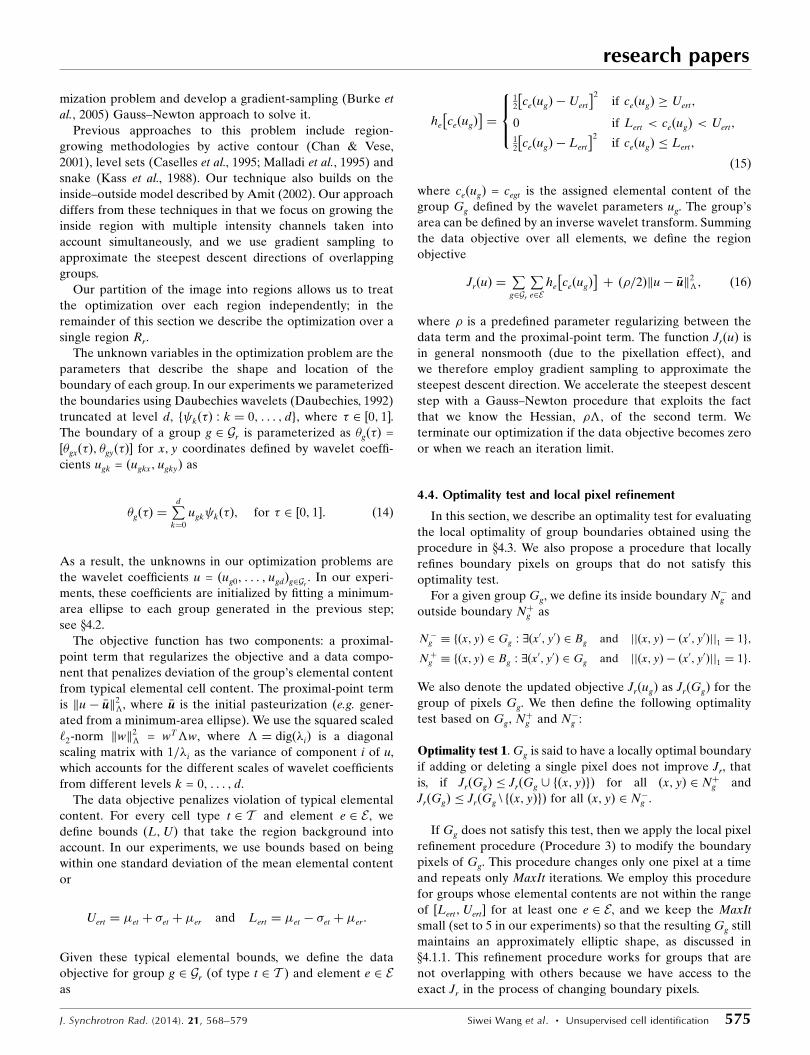
Figure 4Example of the progress of group merging and deleting operations. (a)Initial configuration; (b), (c) merging two red blood cell groups;(d), (e), (g) merging two yeast cell groups; ( f ) deleting a yeast cell group.The overlay of Mn (green), Fe (red) and Zn (blue) elemental maps (h)shows that this area contains four red blood cells and one yeast cell, whichoverlaps one of the red blood cells. The end configuration in (g) showsthat the estimation procedure identifies this configuration correctly.Group boundaries are shown as ellipses for illustration only; alloperations are based on taking the union of pixels.

mization problem and develop a gradient-sampling (Burke et

al., 2005) Gauss–Newton approach to solve it.

Previous approaches to this problem include region-

growing methodologies by active contour (Chan & Vese,

2001), level sets (Caselles et al., 1995; Malladi et al., 1995) and

snake (Kass et al., 1988). Our technique also builds on the

inside–outside model described by Amit (2002). Our approach

differs from these techniques in that we focus on growing the

inside region with multiple intensity channels taken into

account simultaneously, and we use gradient sampling to

approximate the steepest descent directions of overlapping

groups.

Our partition of the image into regions allows us to treat

the optimization over each region independently; in the

remainder of this section we describe the optimization over a

single region Rr.

The unknown variables in the optimization problem are the

parameters that describe the shape and location of the

boundary of each group. In our experiments we parameterized

the boundaries using Daubechies wavelets (Daubechies, 1992)

truncated at level d, f kð�Þ : k ¼ 0; . . . ; dg, where � 2 ½0; 1�.

The boundary of a group g 2 Gr is parameterized as �gð�Þ =

½�gxð�Þ; �gyð�Þ� for x; y coordinates defined by wavelet coeffi-

cients ugk = ðugkx; ugkyÞ as

�gð�Þ ¼Pdk¼0

ugk kð�Þ; for � 2 ½0; 1�: ð14Þ

As a result, the unknowns in our optimization problems are

the wavelet coefficients u = ðug0; . . . ; ugdÞg2Gr. In our experi-

ments, these coefficients are initialized by fitting a minimum-

area ellipse to each group generated in the previous step;

see x4.2.

The objective function has two components: a proximal-

point term that regularizes the objective and a data compo-

nent that penalizes deviation of the group’s elemental content

from typical elemental cell content. The proximal-point term

is ku� �uuk2�, where �uu is the initial pasteurization (e.g. gener-

ated from a minimum-area ellipse). We use the squared scaled

‘2-norm kwk2� = wT�w, where � ¼ digð�iÞ is a diagonal

scaling matrix with 1=�i as the variance of component i of u,

which accounts for the different scales of wavelet coefficients

from different levels k = 0; . . . ; d.

The data objective penalizes violation of typical elemental

content. For every cell type t 2 T and element e 2 E, we

define bounds ðL;UÞ that take the region background into

account. In our experiments, we use bounds based on being

within one standard deviation of the mean elemental content

or

Uert ¼ �et þ �et þ �er and Lert ¼ �et � �et þ �er:

Given these typical elemental bounds, we define the data

objective for group g 2 Gr (of type t 2 T ) and element e 2 E

as

he ceðugÞ� �

¼

12 ceðugÞ � Uert

� �2if ceðugÞ � Uert;

0 if Lert < ceðugÞ < Uert;12 ceðugÞ � Lert

� �2if ceðugÞ Lert;

8><>:

ð15Þ

where ceðugÞ = cegt is the assigned elemental content of the

group Gg defined by the wavelet parameters ug. The group’s

area can be defined by an inverse wavelet transform. Summing

the data objective over all elements, we define the region

objective

JrðuÞ ¼P

g2Gr

Pe2E

he ceðugÞ� �

þ ð=2Þku� �uuk2�; ð16Þ

where is a predefined parameter regularizing between the

data term and the proximal-point term. The function JrðuÞ is

in general nonsmooth (due to the pixellation effect), and

we therefore employ gradient sampling to approximate the

steepest descent direction. We accelerate the steepest descent

step with a Gauss–Newton procedure that exploits the fact

that we know the Hessian, �, of the second term. We

terminate our optimization if the data objective becomes zero

or when we reach an iteration limit.

4.4. Optimality test and local pixel refinement

In this section, we describe an optimality test for evaluating

the local optimality of group boundaries obtained using the

procedure in x4.3. We also propose a procedure that locally

refines boundary pixels on groups that do not satisfy this

optimality test.

For a given group Gg, we define its inside boundary N�g and

outside boundary Nþg as

N�g � fðx; yÞ 2 Gg : 9ðx0; y0Þ 2 Bg and jjðx; yÞ � ðx0; y0Þjj1 ¼ 1g;

Nþg � fðx; yÞ 2 Bg : 9ðx0; y0Þ 2 Gg and jjðx; yÞ � ðx0; y0Þjj1 ¼ 1g:

We also denote the updated objective JrðugÞ as JrðGgÞ for the

group of pixels Gg. We then define the following optimality

test based on Gg, Nþg and N�g :

Optimality test 1. Gg is said to have a locally optimal boundary

if adding or deleting a single pixel does not improve Jr, that

is, if JrðGgÞ JrðGg [ fðx; yÞgÞ for all ðx; yÞ 2 Nþg and

JrðGgÞ JrðGg \ fðx; yÞgÞ for all ðx; yÞ 2 N�g .

If Gg does not satisfy this test, then we apply the local pixel

refinement procedure (Procedure 3) to modify the boundary

pixels of Gg. This procedure changes only one pixel at a time

and repeats only MaxIt iterations. We employ this procedure

for groups whose elemental contents are not within the range

of ½Lert;Uert� for at least one e 2 E, and we keep the MaxIt

small (set to 5 in our experiments) so that the resulting Gg still

maintains an approximately elliptic shape, as discussed in

x4.1.1. This refinement procedure works for groups that are

not overlapping with others because we have access to the

exact Jr in the process of changing boundary pixels.

research papers

J. Synchrotron Rad. (2014). 21, 568–579 Siwei Wang et al. � Unsupervised cell identification 575

Procedure 3. Local pixel refinement (see x4.4).

Given pixel sets Gg, N�g and Nþg ;

for iter < MaxIt do

Let ðxþ; yþÞ ¼ argminðx;yÞ2Nþg

JrðGg [ fðx; yÞgÞ

and set Jþr ¼ JrðGg [ fðxþ; yþÞgÞ;

Let ðx�; y�Þ ¼ argminðx;yÞ2N�g

JrðGg \ fðx; yÞgÞ

and set J�r ¼ JrðGg \ fðx�; y�ÞgÞ;

if JrðGgÞ minðJþr ; J�r Þ then

Locally optimal: return;

else if J�r < Jþr then

Remove pixel ðx�; y�Þ from Gg;

else

Add pixel ðxþ; yþÞ to Gg;

iter = iter + 1.

5. Results

In this section, we present the results obtained from applying

our approach to the test data set described in x3. Since the

focus of using X-ray fluorescent microscopy is to study

elemental contents of cells and we do not have manual

annotations to compare with individual cells, our key metric of

success is how well the elemental content distributions of the

identified cell populations match the truncated Gaussian with

their means represented by elemental content based on hand-

drawn ROIs.

We evaluate the resulting cell populations based on the

elemental distributions of each cell’s characteristic elements

and multiple elements of well measurable quantities (e.g. yeast

cells contain P, K, Zn, etc.). In addition, we are interested

in how different the elemental contents from identified cell

populations comparing with those from the hand-drawn ROIs,

especially if these ROIs are informative enough for identifying

the entire cell population. We expect contents of well

measurable elements in given cell populations to be well

above the estimated background derived from neighboring

background pixels (x4.1.2) in their respective cell populations.

Hence, as a byproduct, we also evaluate how well the back-

ground estimation works.

In Fig. 5, we show color-coded elemental content distribu-

tions (P, K, Mn, Fe, Zn) for the three cell types. These

elemental distributions are the net contents after removal of

estimated background. We also include an additional row

showing the estimated background distributions. We observe

the following:

(i) If a cell population contains well measurable amounts of

specific elements, then the corresponding net contents (after

removing background using neighbor background pixels) are

well above zero. For example, the characteristic elements (Mn,

Fe and Zn) are distinctly high in their respective cell popu-

lations; yeast cells also show high contents in P and K simul-

taneously. For those elements whose contents in cells are close

to detection limits, their net content distributions can have

both positive and negative values. This is because (a) the

statistical nature of the collected signal can lead to negative

numbers when two nearly equal signals are subtracted; (b)

some of these elements contain ‘halo’ regions: if the identified

cells do not contain large quantities of these elements and they

are inside of these regions (e.g. K content in red blood cells),

we can obtain negative net contents.

(ii) The distances between the magenta and black lines

show how much the initial guesses from a few hand-drawn

ROIs differ from the means of the cell populations determined

by our method. The mean contents from the identified cell

populations (>100 cells) are within 20% ranges compared with

the mean contents from hand-drawn ROIs, which include no

more than ten cells. This indicates that the cell populations in

our dataset have consistent elemental contents, especially in

their respective characteristic elements.

(iii) We observe that the iron content values we obtained

are in a reasonably good agreement with literature values. For

example, for red blood cells we measure a mean Fe content of

about 50 fg per cell (see Fig. 5), which compares with 60–80 fg

per cell as reported by Jones (1975) and Hewitt et al. (1989).

The difference may be due to possible elemental redistribu-

tion due to the sample preparation procedure, the limited

statistics we employed, an underestimate of cell size, or an

overestimate of background contribution.

To summarize, we observe that all identified cells have

significant contents that match their respective biological

expectations. These elemental contents are different from the

mean contents of the hand-drawn ROIs by about 20%.

Furthermore, our background estimation works well for

research papers

576 Siwei Wang et al. � Unsupervised cell identification J. Synchrotron Rad. (2014). 21, 568–579

Figure 5P, K, Mn, Fe, Zn content distributions of identified algae (green), yeast(blue) and red blood (red) cells. The light blue, pink and light greenpoints indicate the estimated background (Bg) contents of the respectivecell areas. The horizontal axis (log scale) shows net elemental content,and the points are distributed randomly within bounds in the verticaldirection in order to provide separation. The magenta and black linesshow, respectively, the initialized means from hand-drawn regions ofinterest, and the means of the actual cell populations in the characteristicelements. As expected, the cells tend to have high elemental content intheir characteristic elements: red blood cells have high Fe content, andyeast cells contain significant amounts of P and Zn. Some elements canshow negative content for some cells (the K channel in red blood cells,for example); this is because of the need to subtract substrate andbackground signals from the raw elemental content to calculate the actualelemental content for a given cell. In case the signal is close to zero, thestatistical nature of the collected signal can lead to negative numberswhen two nearly equal signals are subtracted.

elements with well measurable amounts in given cell popula-

tions.

6. Discussion and validation

The cell identification results we report in x5 use the sum of

the four detector measurements, where each detector segment

records the fluorescence signal from a slightly different

viewing angle. This can lead to slight variations in calculated

elemental concentration because of variations in scattering

background and absorption of fluorescence signal along the

viewing path. To validate that the identified cell areas do

contain cells, we applied this approach to each elemental

concentration map separately and compared the elemental

distributions of all resulting cell populations. Our assumption

is that if an area contains actual cells, all four detectors will

measure significant elemental signals from it. In this case, if

our approach identifies similar cells from all four individual

measurements and the sum of them, this identification

agreement provides evidence that our approach finds cells

correctly.

Fig. 6 shows the elemental content from the resulting red

blood and yeast cells (there are only five algae cells). These

scatterplots show that the Fe distributions of resulting red

blood cells and the Zn distributions of resulting yeast cells are

similar. An ANOVA test (Rice, 1995) determines that none of

the five cell populations has statistically significant differences

in elemental distribution. Hence we conclude that this iden-

tification approach using different measurements of the same

sample recognizes similar elemental distributions of each

resulting cell population.

We also examined the dependence on the initial determi-

nation of foreground and background regions. In the

preprocessing step, we divide pixels into foreground and

background components based on the thresholding pixel

intensity in the their characteristic elemental maps. We eval-

uate the robustness of our approach by varying the threshold

20%. This thresholding variation changes the initial group

configurations.

We would like to evaluate whether we can obtain similar

cell identification results using initial group configurations

from these three different thresholds. If we obtain similar cell

identification result, we believe that our approach is robust

with respect to threshold variation in the 20% range.

The up/down thresholding changes the number of initial

groups (‘Initial’ in Fig. 7) by 15–20%, whereas the numbers of

cells among all resulting cell populations (‘Result’ in Fig. 7)

differ only by 5–8%. For example, the preprocessing proce-

dure obtains 288 initial yeast cell groups using the original

threshold, and there are 197 yeast cells in the resulting

cell population; using downthresholding, the preprocessing

obtains 347 initial (a 20% difference) and 209 final (a 6%

difference) yeast cell groups. These results illustrate that our

research papers

J. Synchrotron Rad. (2014). 21, 568–579 Siwei Wang et al. � Unsupervised cell identification 577

Figure 8Boxplots showing (a) Fe distributions in red blood cell populations and(b) Zn distributions in yeast cell populations resulting from threedifferent initial elemental thresholding choices. The similarity of resultsshows that the results obtained are robust against changes in initialparameters. The central mark is the median, the edges of the boxesdenote the 25th and 75th percentiles, the whiskers extend to the mostextreme data points not considered outliers, and the outliers are plottedindividually.

Figure 6(a) Boxplot of Fe distributions from red blood cells obtained using theseparate detector segments as well as their sum. (b) Boxplot of Zndistributions from yeast cells obtained using separate detector segmentsas well as their sum. This figure demonstrates that elemental contentsobtained by separate analysis from the different detector segments aresimilar, adding confidence in the robustness of our results. The centralmark is the median, the edges of the boxes denote the 25th and 75thpercentiles, the whiskers extend to the most extreme data points notconsidered outliers, and the outliers are plotted individually.

Figure 7Test of the total number of red blood cells (a) and yeast cells (b) identifiedas the initial choice for elemental thresholding is changed over a 20%range. Of course the initial threshold choice has a strong direct effect onthe initial number of putative cells found by the algorithm. The effect ofthis initial parameter choice is greatly reduced at the end of our analysissequence, as is shown by the comparative robustness of the resulting cellnumber.

final cell populations are relatively insensitive to the different

thresholding; the final results change only by 8%.

We also compare the elemental contents of cell populations

resulting from the three different initial threshold choices. The

scatterplots in Fig. 8 show that both the Zn distributions of the

resulting yeast cell populations and Fe distributions of the

resulting red blood cells are insensitive to the different

thresholding. Furthermore, we found no significant difference

in the means of all three Zn (and Fe) distributions using a one-

way ANOVA test.

These results show that our approach is able to estimate

elemental content of cell populations very well, with final

results being insensitive to modest changes in initial input

parameters.

7. Conclusion and future work

We describe here an approach for identifying cells of complex

configurations (including heavily overlapping cells) in multi-

dimensional XFM datasets. Without explicit expert knowledge

and training using manual annotation, we demonstrate that

this approach can identify and differentiate multiple cell types

based on their respective trace elemental content. The

generalized likelihood ratio test is robust in determining cell

configurations using initial putative groups generated by using

various elemental content thresholds. Furthermore, our

approach shows consistent performance in processing regions

with overlapping structures, where it is difficult or impossible

to obtain reliable cell identification manually, and easily deals

with the volume and complexity of current microscopy data.

On a large dataset such as the test dataset shown here, our

algorithm takes about an hour of total processing time on a

personal laptop, with segmentation taking about 5 min, esti-

mation of regions about 45 min, and boundary delineation and

pixel refinement another 10 min. The computing time scales

linearly with the number of regions, and exponentially with

the number of cells in each region. (This is ten times faster

compared with the MAPS routine in obtaining fitted data.

Also, our segmentation runs in seconds, which is comparable

with running the ‘analyze particle’ routine in ImageJ.)

As we discussed in x1, our method extends other unsuper-

vised cell identification methods in that we incorporate into

the likelihood test as many independent elements simulta-

neously as needed, and model overlapping cells to determine

their respective elemental content. For example, the common

cell counting routine ‘analyze particles’ in ImageJ (Abramoff

et al., 2004) only processes one independent intensity channel

at a time, whereas we use all nine elemental maps simulta-

neously to determine cells. In addition, its approach to cell

shape estimation, namely the generation of cell segments

based on the thresholding and subsequent clustering based on

pixel positions, is similar to our preprocessing segmentation.

Our approach extends this by effectively incorporating cell

properties such as total elemental content and cell

morphology to identify whole cells (i.e. noncontiguous nearby

pixels are not mistakenly identified as multiple cells).

Extensions that we plan to integrate into this methodology

include the modeling of cell size and shape, adapting the

covariance matrix according to the cell size, and in particular

making this approach iterative so that the result from the pixel

refinement is fed back to the estimation of group configura-

tions to further improve the identification. From the compu-

tational perspective, our next step will be to exploit the mutual

independence of regions to parallelize our algorithm, as well

as to optimize the code for processing speed.

We are aware that this test dataset contains cells with

distinct elemental contents. This condition simplifies the

initialization part of our cell identification. A natural exten-

sion would be to expand the scope of our algorithm in order to

study more complicated cases, including cells with arbitrary

shapes, sizes and heterogeneous (i.e. non-Gaussian) elemental

content distributions, and to analyze full XFM spectra. In

addition, we are interested in developing metrics to measure

quantitatively the performance of this type of unsupervised

approach, possibly aided by image registration with other

types of images (e.g. from optical microscopy).

This work was supported by the US Department of Energy,

Office of Science, Advanced Scientific Computing Research,

and Basic Energy Sciences program (DE-AC02-06CH11357).

We thank Qiaoling Jin and Sophie-Charlotte Gleber for

helpful suggestions. We are grateful for comments from the

referees, which have helped the presentation.

References

Abramoff, M. D., Magelhaes, P. J. & Ram, S. J. (2004). Biophoton. Intl,11, 36–42.

Amit, Y. (2002). 2D Object Detection and Recognition: Models,Algorithms and Networks. Cambridge: MIT Press.

Arteta, C., Lempitsky, V., Noble, J. A. & Zisserman, A. (2012).Proceedings of the 15th International Conference on Medical ImageComputing and Computer-Assisted Intervention (MICCAI12), pp.348–356. Berlin: Springer-Verlag.

Aydin, Z., Murray, J., Waterston, R. & Noble, W. (2010). BMCBioinformatics, 11, 1–13.

Bergeest, J.-P. & Rohr, K. (2011). Lect. Notes Comput. Sci. 6891, 645–652.

Bergeest, J.-P. & Rohr, K. (2012). Med. Image Anal. 16, 1436–1444.Burke, J. V., Lewis, A. S. & Overton, M. L. (2005). SIAM J. Optim. 15,

751–779.Caselles, V., Kimmel, R. & Sapiro, G. (1995). Intl J. Comput. Vis. 22,

61–79.Chan, T. & Vese, L. (2001). IEEE Trans. Image Process. 10, 266–277.Cortes, L. & Amit, Y. (2008). IEEE Trans. Pattern Anal. Mach. Intell.

30, 1998–2010.Daubechies, I. (1992). Ten Lectures on Wavelets, CBMS-NSF

Regional Conference Series in Applied Mathematics. Philadelphia:SIAM.

Dhillon, I., Guan, Y. & Kulis, B. (2007). IEEE Trans. Pattern Anal.Mach. Intell. 29, 1944–1957.

Dismukes, G. C. (1986). Photochem. Photobiol. 43, 99–115.Good, N. E., Winget, G. D., Winter, W., Connolly, T. N., Izawa, S. &

Singh, R. M. (1966). Biochemistry, 5, 467–477.Gorman, D. S. & Levine, R. P. (1965). Proc. Natl Acad. Sci. USA, 54,

1665–1669.Hawkins, W. W., Speck, E. & Leonard, V. G. (1954). Blood, 9, 999–

1007.

research papers

578 Siwei Wang et al. � Unsupervised cell identification J. Synchrotron Rad. (2014). 21, 568–579

Hewitt, C., Innes, D., Savory, J. & Wills, M. (1989). Clin. Chem. 35,1777–1779.

Jones, R. (1975). Lab. Anim. 9, 143–147.Kass, M., Witkin, A. & Terzopoulos, D. (1988). Intl J. Comput. Vis. 1,

321–331.Kasson, P. M., Huppa, J. B., Davis, M. M. & Brunger, A. T. (2005).

Bioinformatics, 21, 3778–3786.Kirz, J. (1980). Ultrasoft X-ray Microscopy: Its Application to

Biological and Physical Sciences, edited by D. F. Parsons, Annalsof the New York Academy of Sciences, pp. 273–287. New York,USA.

Lerotic, M., Jacobsen, C., Gillow, J., Francis, A., Wirick, S., Vogt, S. &Maser, J. (2005). J. Electron Spectrosc. Relat. Phenom. 144–147,1137–1143.

Lerotic, M., Jacobsen, C., Schafer, T. & Vogt, S. (2004). Ultramicro-scopy, 100, 35–57.

Lin, G., Adiga, U., Olson, K., Guzowski, J. F., Barnes, C. A. &Roysam, B. (2003). Cytometry A, 56A, 23–36.

Ljosa, V. & Carpenter, A. E. (2009). PLoS Comput. Biol. 5, e1000603.Lundblad, V. & Struhl, K. (2001). Current Protocols in Molecular

Biology, pp. 13.0.1–13.0.4. Hoboken: John Wiley.McCullough, D. P., Gudla, P. R., Harris, B. S., Collins, J. A., Meaburn,

K. J., Nakaya, M. A., Yamaguchi, T. P., Misteli, T. & Lockett, S. J.(2008). IEEE Trans. Med. Imaging, 27, 723–734.

Malladi, R., Sethian, J. & Vemuri, B. (1995). IEEE Trans. PatternAnal. Mach. Intell. 17, 158–175.

Marvin, R., Wolford, J., Kidd, M., Murphy, S., Ward, J., Que, E.,Mayer, M., Penner-Hahn, J., Haldar, K. & O’ Halloran, T. (2012).Chem. Biol. 19, 731–741.

Paunesku, T., Vogt, S., Maser, J., Lai, B. & Woloschak, G. (2006).J. Cell. Biochem. 99, 1489–1502.

Plaza, A., Martinez, P., Perez, R. & Plaza, J. (2004). Pattern Recognit.37, 1097–1116.

Rice, J. A. (1995). Mathematical Statistics and Data Analysis, 2nd ed.Belmon: Duxbury Press.

Russell, C., Metaxas, D., Restif, C. & Torr, P. (2007). 2007 IEEEInternational Conference on Computer Vision, pp. 2362–2369.

Ryan, C., van Achterbergh, E., Yeats, C., Win, T. T. & Cripps, G.(2002). Nucl. Instrum. Methods Phys. Res. B, 189, 400–407.

Sole, V., Papillon, E., Cotte, M., Walter, P. & Susini, J. (2007).Spectrochim. Acta B, 62, 63–68.

Swedlow, J. R., Goldberg, I. G. & Eliceiri, K. W. (2009). Annu. Rev.Biophys. 38, 327–346.

Tan, M., Braga, R. A., Fink, R. W. & Rao, P. V. (1982). Phys. Scr. 25,536.

Tao, C. Y., Hoyt, J. & Feng, Y. (2007). J. Biomol. Screen. 12, 490–496.

Vogt, S. (2003). J. Phys. IV, 104, 635–638.Wang, M., Zhou, X., Li, F., Huckins, J., King, R. W. & Wong, S. T. C.

(2007). Bioinformatics, 24, 94–101.Wasserman, L. (2003). All of Statistics: A Concise Course in Statistical

Inference. Berlin: Springer.Wolz, R., Heckemann, R. A., Aljabar, P., Hajnal, J. V., Hammers,

A., Lotjonen, J. & Rueckert, D. (2010). NeuroImage, 52, 109–118.

Wu, B. & Nevatia, R. (2009). Intl J. Comput. Vis. 82, 185–204.Yin, Z., Bise, R., Chen, M. & Kanade, T. (2010). IEEE International

Symposium on Biomedical Imaging (ISBI), pp. 125–128.

research papers

J. Synchrotron Rad. (2014). 21, 568–579 Siwei Wang et al. � Unsupervised cell identification 579