Unstructured Jumps and Compressed Size as Defect ... · 3 Structured Gotos are ... as software engineering metrics, ... routine maintenance and two other metrics of software development

Unstructured Jumps and CompressedSize as Defect-Prediction Metrics

Eli Sennesh

Technion - Computer Science Department - M.Sc. Thesis MSC-2015-09 - 2015


Unstructured Jumps and CompressedSize as Defect-Prediction Metrics

Research Thesis

Submitted in partial fulfillment of the requirements

for the degree of Master of Science in Computer Science

Eli Sennesh

Submitted to the Senate

of the Technion — Israel Institute of Technology Shvat

5775 Haifa February 2015



This research was carried out under the supervision of Prof. Yossi Gil, in the Faculty of Computer

Science.

ACKNOWLEDGEMENTS

My most heartfelt thanks to my parents for always encouraging me, to my advisor Yossi for

never giving up on me, and my fiancee Alexa for never doing the sensible thing and leaving.

The Technion’s funding of this research is hereby acknowledged.



Contents

List of Figures

List of Tables

Abstract 1

1 Introduction 31.1 Questions and Contributions . . . . . . . . . . . . . . . . . . . . . . . . . . . 7

2 Preliminaries 92.1 Code Corpora . . . . . . . . . . . . . . . . . . . . . . . . . . . . . . . . . . . 9

2.1.1 Corpus Selection Process . . . . . . . . . . . . . . . . . . . . . . . . . 9

2.2 Metrics . . . . . . . . . . . . . . . . . . . . . . . . . . . . . . . . . . . . . . 11

2.2.1 Independent Variables: Code Metrics . . . . . . . . . . . . . . . . . . 11

2.2.2 Dependent Variables: Metrics for Development Effort . . . . . . . . . 13

2.2.3 Distribution of Code Metrics . . . . . . . . . . . . . . . . . . . . . . . 14

2.3 Statistical Tests . . . . . . . . . . . . . . . . . . . . . . . . . . . . . . . . . . 14

2.3.1 Kendall’s τb correlation coefficient . . . . . . . . . . . . . . . . . . . . 14

3 Structured Gotos are (Slightly) Harmful 173.1 Initial Hypotheses . . . . . . . . . . . . . . . . . . . . . . . . . . . . . . . . . 17

3.2 Preliminary χ2 Tests . . . . . . . . . . . . . . . . . . . . . . . . . . . . . . . 17

3.3 Predictive power of code metrics . . . . . . . . . . . . . . . . . . . . . . . . . 18

3.3.1 Metrics predicting Defects . . . . . . . . . . . . . . . . . . . . . . . . 18

3.3.2 Metrics predicting Churn . . . . . . . . . . . . . . . . . . . . . . . . . 18

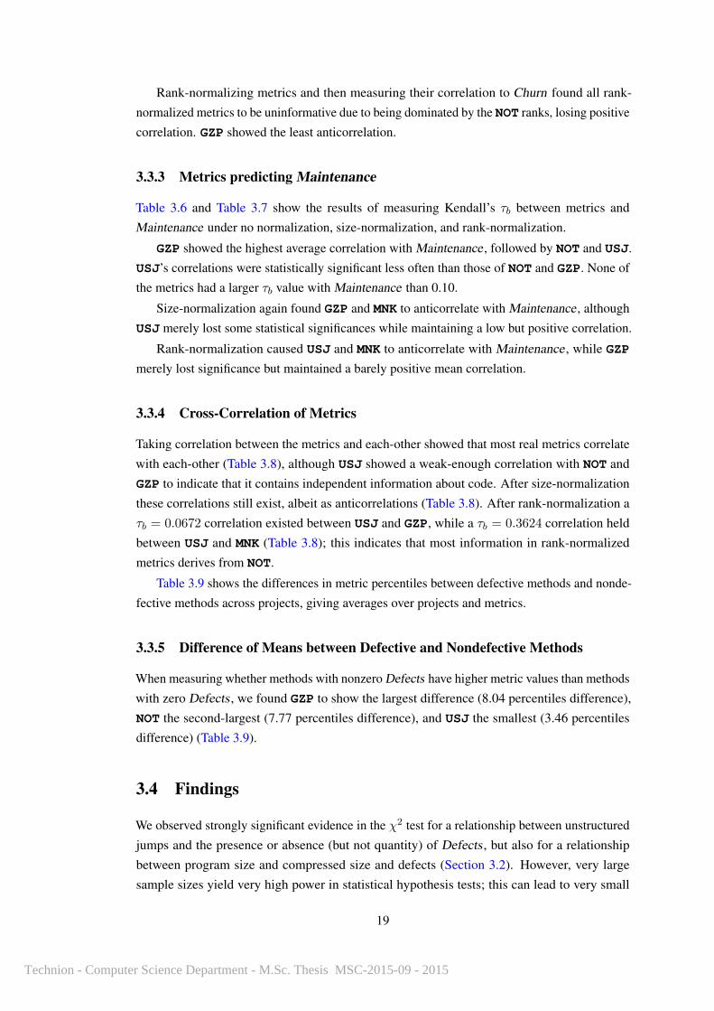
3.3.3 Metrics predicting Maintenance . . . . . . . . . . . . . . . . . . . . . 19

3.3.4 Cross-Correlation of Metrics . . . . . . . . . . . . . . . . . . . . . . . 19

3.3.5 Difference of Means between Defective and Nondefective Methods . . 19

3.4 Findings . . . . . . . . . . . . . . . . . . . . . . . . . . . . . . . . . . . . . . 19

4 The Rediscovery of the Bug-Density Paradox 294.1 Prior Expectations . . . . . . . . . . . . . . . . . . . . . . . . . . . . . . . . . 29

4.2 Related Work . . . . . . . . . . . . . . . . . . . . . . . . . . . . . . . . . . . 30


4.3 Densities Plotted and Correlations Measured . . . . . . . . . . . . . . . . . . . 31

4.3.1 Cumulative Defect Likelihood functions . . . . . . . . . . . . . . . . . 31

4.3.2 Empirical Defect Densities . . . . . . . . . . . . . . . . . . . . . . . . 33

4.3.3 Predictive Power of Metric Values for Defect Densities . . . . . . . . . 37

4.3.4 A Transformed Metric for Flat Defect Density . . . . . . . . . . . . . 37

4.3.5 The Transformed Metric’s Predictive Power . . . . . . . . . . . . . . . 39

4.4 Discussion . . . . . . . . . . . . . . . . . . . . . . . . . . . . . . . . . . . . . 40

5 Conclusion and open questions 495.1 Gotos are Sometimes Somewhat Harmful . . . . . . . . . . . . . . . . . . . . 49

5.2 Defects are Concentrated in Smaller Methods . . . . . . . . . . . . . . . . . . 50

Hebrew Abstract i


List of Figures

1.1 Prominent entry to 1987 International Obfuscated C Contest . . . . . . . . . . 4

1.2 An example of using labeled break and continue to write unstructured

jumps in Java . . . . . . . . . . . . . . . . . . . . . . . . . . . . . . . . . . . 5

4.1 In a model where each token in a method has an independent chance of contain-

ing a defect, the cumulative probability of the method as a whole containing a

defect eventually rises to unity. . . . . . . . . . . . . . . . . . . . . . . . . . . 30

4.2 Cumulative probability method contains a defect vs NOT percentiles . . . . . . 32

4.3 Cumulative probability method contains a defect vs GZP percentiles . . . . . . 32

4.4 Defects per token (absolute defect density) vs. NOT . . . . . . . . . . . . . . . 33

4.5 Defects per compressed byte (absolute defect density) vs. GZP . . . . . . . . . 34

4.6 Defects per token rank percentile (relative defect density) vs. NOT percentiles . 35

4.7 Defects per compressed byte rank percentile (relative defect density) vs. GZP

percentiles . . . . . . . . . . . . . . . . . . . . . . . . . . . . . . . . . . . . . 36

4.8 Mean Kendall’s τb over all projects of defect density with respect to the metric

raised to a power ε vs ε . . . . . . . . . . . . . . . . . . . . . . . . . . . . . . 38

4.9 Mean Kendall’s τb value over all projects of defect density with respect to the

metric plugged into the formula nlogε(n) vs ε . . . . . . . . . . . . . . . . . . 39



List of Tables

2.1 Software corpora constituting the dataset (in descending number of source

files inspected), and information on the sampled time-frame and the number of

developers involved . . . . . . . . . . . . . . . . . . . . . . . . . . . . . . . . 10

2.2 Essential statistics on the size and commit history of the corpora in our dataset

(in descending order by number of files inspected) . . . . . . . . . . . . . . . . 12

2.3 p-values from the Kolmogorov-Smirnov test of uniformity for metric values . . 16

3.1 p-values for the χ2 test of independence between methods with defect Proneness

of 1 and methods with defect Proneness of 0 . . . . . . . . . . . . . . . . . . . 22

3.2 Predictability of Defects from unnormalized metric values, measured by Kendall’s

τb. Values range between -1.0 and 1.0. . . . . . . . . . . . . . . . . . . . . . . 22

3.3 Predictability of Defects from size-normalized and rank-normalized metric

values, measured by Kendall’s τb. Values range between -1.0 and 1.0. . . . . . 23

3.4 Predictability of Churn from unnormalized metric values, measured by Kendall’s

τb. Values range between -1.0 and 1.0. . . . . . . . . . . . . . . . . . . . . . . 24

3.5 Predictability of Churn from size-normalized and rank-normalized metric values,

measured by Kendall’s τb. Values range between -1.0 and 1.0. . . . . . . . . . 25

3.6 Predictability of Maintenance from unnormalized metric values, measured by

Kendall’s τb. Values range between -1.0 and 1.0. . . . . . . . . . . . . . . . . . 26

3.7 Predictability of Maintenance from size-normalized and rank-normalized metric

values, measured by Kendall’s τb. Values range between -1.0 and 1.0. . . . . . 27

3.8 Predictability of unnormalized, size-normalized, and rank-normalized metric

values from each-other (from left to right), measured by Kendall’s τb. Values

range from -1.0 to 1.0. . . . . . . . . . . . . . . . . . . . . . . . . . . . . . . 27

3.9 Defective methods have a mean percentile metric-value several percentage

points higher than that of non-defective methods. . . . . . . . . . . . . . . . . 28

4.1 p-values for the Kolmogorov-Smirnov test of uniformity for metric densities . . 42

4.2 Mean defect densities at individual size-metric values across corpora . . . . . . 42

4.3 Mean defect densities at size-metric percentiles across corpora . . . . . . . . . 42

4.4 Predictability of defect density from size-metric values, measured by Kendall’s

τb. Values range between -1.0 to 1.0. . . . . . . . . . . . . . . . . . . . . . . . 43


4.5 Predictability of defect Proneness from size metrics and size metrics transformed

by f(n) = nlog−5.9(n), measured by Kendall’s τb. Values range from -1.0 to 1.0. 44

4.6 Predictability of Defects from size metrics and size metrics transformed by

f(n) = nlog−5.9(n), measured by Kendall’s τb. Values range from -1.0 to 1.0. . 45

4.7 Predictability of Churn from size metrics and size metrics transformed by


4.8 Predictability of Versions from size metrics and size metrics transformed by


4.9 Predictability of Maintenance from size metrics and size metrics transformed

by f(n) = nlog−5.9(n), measured by Kendall’s τb. Values range from -1.0 to 1.0. 48


Abstract

With the advent of easier to parse languages such as Java, and the availability on the Internet of

open-source software repositories, complete with versioning histories, empirical studies at scale

of software engineering metrics and measurements have become possible and feasible.

We take up the questions of if and how “structured goto” statements impact defect prone-

ness, and of which what concept of size yields a superior metric for defect prediction. We view

the topic through the lens of evidence-based language design, following the drive ignited by

Markstrum [22].

Both the goto keyword and large methods are traditionally “considered harmful,” so much

so that programmers are advised to avoid them in all cases. Despite this traditional view, modern

languages still contain constructs for branching to nonadjacent syntax-tree nodes, which we

term unstructured jumps. We count these goto-like unstructured jumps, alongside method size

and compressed method size, as software engineering metrics, and examine the evolution of

26 open-source code corpora in relation to those metrics. We employ five different measures

of defectiveness and development effort. We measure the statistical quality of our metrics as

predictors of our defect measurements.

We show that the number of unstructured jumps is a predictor of defects, routine maintenance

and two other metrics of software development effort. The correlation between unstructured

jumps and development effort is positive, and it remains so even after accounting for the effect

of code size. We also show that between uncompressed and compressed code size, compressed

size is the superior predictor of defect proneness, maintenance, version increase, and code churn,

while uncompressed size only predicts better when measuring accumulated defects.

The number of unstructured jumps is superior to code size, both compressed and uncom-

pressed, in its predictive power of accumulated defects. Compressed size, however, provides

the best predictor for churn and routine maintenance. Uncompressed size provides the best

predictor for the density of defects throughout methods of fixed size.

We also find that size metrics do not predict defects as a linear function of method size.

Defect density, the quantity of defects per unit of method size, is nonuniform across method

lengths, and displays a statistically significant negative correlation with method length overall.

When relative method size is considered instead of absolute method size, we find that defects

cluster densely in the smallest and largest methods, with very low defect densities in between.

Attempts to propose a transformation on a size metric which would yield a new, metric

with constant defect density, contrary to expectations, yielded strictly worse predictors than the

1


original size metrics.

2


Chapter 1

Introduction

Anecdotally, the presence of a single extra goto statement in C [16] code recently caused a

major software failure 1. This anecdote can scarcely help but bring to mind the ancient debate

on the goto construct. In this research, we further debate and revisit debate this issue.

Dijkstra advocated eliminating goto statements from code as early as 1968 [10], holding

that its usage

“has an immediate consequence that it becomes terribly hard to find any meaningful

set of coordinates in which to describe the process progress.”

To give an example of how goto can make programs difficult to reason about, we present

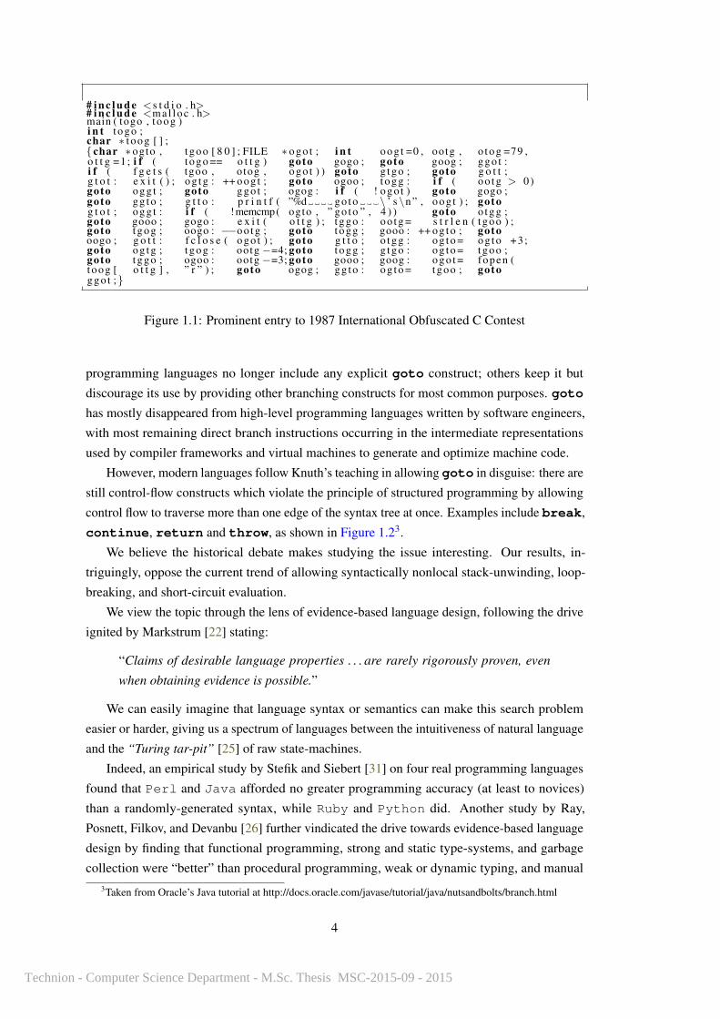
the entry noted for “Worst Style” in the 1987 International Obfuscated C Contest in Figure 1.1.

It purportedly (we have not actually run it) “[C]ounts goto’s, all ids anagrams of ‘goto’, all

flow w goto” [sic]2.

“Structured programming”, in contrast, consists in having control flow only through adjacent

nodes in the abstract syntax tree.

The case against goto usage is not limited to mere argumentation. goto increases a

program’s cyclomatic complexity [23]. It makes control-flow graphs irreducible [2], thereby

complicating static analysis and compiler-level optimization of the code. goto statements

are also formally unnecessary, as demonstrated by Bohm and Jacopini [8], whose structured

programming theorem shows how to take any program using goto and construct an equivalent

but structured program without goto.

The primary advantage of goto over higher-level control-flow constructs is its simpler

translation into single, unconditional branch instructions, and thus its greater efficiency. Indeed,

Knuth [17] proposed using goto for exactly this purpose, arguing that certain uses of goto

are in harmony with structured programming. And, in “TEX: the program” [19], the canonical

example of “literate programming” [18], Knuth demonstrated the use of goto to realize more

modern constructs such as continue and return.

Another advocate for goto was Rubin [27], who suggested that goto itself had no effect

on code quality independent of the competence of its users. Despite this claim, most modern1http://www.wired.com/threatlevel/2014/02/gotofail/2http://www.ioccc.org/1987/hines.hint

3


http://www.wired.com/threatlevel/2014/02/gotofail/

http://www.ioccc.org/1987/hines.hint

# i n c l u d e <s t d i o . h># i n c l u d e <ma l l oc . h>main ( togo , t oog )i n t t ogo ;char ∗ t oog [ ] ;{ char ∗ogto , t goo [ 8 0 ] ; FILE ∗ ogo t ; i n t oog t =0 , ootg , o tog =79 ,o t t g =1; i f ( t ogo == o t t g ) goto gogo ; goto goog ; ggo t :i f ( f g e t s ( tgoo , otog , ogo t ) ) goto g tgo ; goto g o t t ;g t o t : e x i t ( ) ; og tg : ++ oog t ; goto ogoo ; togg : i f ( oo tg > 0)goto ogg t ; goto ggo t ; ogog : i f ( ! ogo t ) goto gogo ;goto gg to ; g t t o : p r i n t f ( ”%d go to \ ’ s\n ” , oog t ) ; gotog t o t ; ogg t : i f ( !memcmp( ogto , ” go to ” , 4 ) ) goto o tgg ;goto gooo ; gogo : e x i t ( o t t g ) ; t ggo : oo tg = s t r l e n ( tgoo ) ;goto t gog ; oogo : −−oo tg ; goto t ogg ; gooo : ++ og to ; gotooogo ; g o t t : f c l o s e ( ogo t ) ; goto g t t o ; o tgg : og to = og to +3;goto og tg ; t gog : ootg −=4; goto t ogg ; g tgo : og to = tgoo ;goto t ggo ; ogoo : ootg −=3; goto gooo ; goog : ogo t = fopen (toog [ o t t g ] , ” r ” ) ; goto ogog ; gg to : og to = tgoo ; gotoggo t ;}

Figure 1.1: Prominent entry to 1987 International Obfuscated C Contest

programming languages no longer include any explicit goto construct; others keep it but

discourage its use by providing other branching constructs for most common purposes. goto

has mostly disappeared from high-level programming languages written by software engineers,

with most remaining direct branch instructions occurring in the intermediate representations

used by compiler frameworks and virtual machines to generate and optimize machine code.

However, modern languages follow Knuth’s teaching in allowing goto in disguise: there are

still control-flow constructs which violate the principle of structured programming by allowing

control flow to traverse more than one edge of the syntax tree at once. Examples include break,

continue, return and throw, as shown in Figure 1.23.

We believe the historical debate makes studying the issue interesting. Our results, in-

triguingly, oppose the current trend of allowing syntactically nonlocal stack-unwinding, loop-

breaking, and short-circuit evaluation.

We view the topic through the lens of evidence-based language design, following the drive

ignited by Markstrum [22] stating:

“Claims of desirable language properties . . . are rarely rigorously proven, even

when obtaining evidence is possible.”

We can easily imagine that language syntax or semantics can make this search problem

easier or harder, giving us a spectrum of languages between the intuitiveness of natural language

and the “Turing tar-pit” [25] of raw state-machines.

Indeed, an empirical study by Stefik and Siebert [31] on four real programming languages

found that Perl and Java afforded no greater programming accuracy (at least to novices)

than a randomly-generated syntax, while Ruby and Python did. Another study by Ray,

Posnett, Filkov, and Devanbu [26] further vindicated the drive towards evidence-based language

design by finding that functional programming, strong and static type-systems, and garbage

collection were “better” than procedural programming, weak or dynamic typing, and manual3Taken from Oracle’s Java tutorial at http://docs.oracle.com/javase/tutorial/java/nutsandbolts/branch.html

4


c l a s s ContinueWithLabelDemo {p u b l i c s t a t i c vo id main ( S t r i n g [ ] a r g s ) {

S t r i n g searchMe = ” Look f o r a s u b s t r i n g i n me” ;S t r i n g s u b s t r i n g = ” sub ” ;boolean f o u n d I t = f a l s e ;i n t max = searchMe . l e n g t h ( ) −

s u b s t r i n g . l e n g t h ( ) ;t e s t :

f o r ( i n t i = 0 ; i <= max ; i ++) {i n t n = s u b s t r i n g . l e n g t h ( ) ;i n t j = i ;i n t k = 0 ;whi le ( n−− != 0 ) {

i f ( searchMe . c ha rA t ( j ++) != s u b s t r i n g . c ha r At ( k ++) ) {c o n t i nu e t e s t ;

}}f o u n d I t = t rue ;

break t e s t ;}System . o u t . p r i n t l n ( f o u n d I t ? ” Found i t ” : ” Didn ’ t f i n d i t ” ) ;

}}

Figure 1.2: An example of using labeled break and continue to write unstructured jumpsin Java

memory management. They also found that “the defect proneness of languages in general is not

associated with software domains.” In short, some language designs can in fact make the search

problem easier, often by abstracting away implementation details about which the specification

requires nothing in particular.

In addition to viewing programming to a specification as a search problem, we can view

defect prediction as a classification problem, an approach covered quite well in the existing

literature [29]. Finding good metrics then becomes a problem of selecting and generating

features which yield good classification performance. When choosing from among already

available features, the problem of assembling an optimal feature-set is NP-hard in general [7],

but sorting features by their correlation with the class data, according to some correlation

coefficient, is an accepted heuristic.

In this thesis, we thus study a more modern concept:

Definition 1.0.1. Structured goto (alternately: unstructured jump): jump instructions which

violate the structured programming criterion, giving a syntactic block more than one entry or

exit point, or which jump across multiple edges in the abstract-syntax tree.

We take up the questions of if and how “structured goto” statements impact defect prone-

ness, and of which what concept of size yields a superior metric for defect prediction. Our

contribution is not by haranguing: we treat these “structured goto” statements as a metric and

analyze empirically their correlation with other empirical measures of defects.

The advent of easier to parse languages such as JAVA [3], and the availability on the Internet

of open-source repositories, along with their history, made our study (and many others) not only

possible, but also feasible.

5


Findings We investigate the use of unstructured jumps in a dataset comprised of a variety of

professionally-developed software projects. We show that the number of unstructured jumps

is a predictor of defects, routine maintenance and two other metrics of software development

effort. The correlation between unstructured jumps and development effort is positive, and it

remains so even after accounting for the effect of code size.

Curiously, the number of unstructured jumps is (minutely) superior to code size in its

predictive power of code defects. Among size metrics, GZP better predicts defects overall, while

NOT better predicts the density of defects. Defect density declines overall with respect to both

size metrics, although it declines more quickly with respect to NOT than with respect to GZP.

Curiously, when viewed in terms of metric percentiles instead of raw metric values, defects

appear to be clustered into the shortest and longest methods, with very little defect density in

the middle ranges of method sizes; this effect occurs with respect to both size metrics.

Based on these findings, we argue that unstructured jumps, which are already more structured

than goto, display a harmful impact on defect rates. Our findings point against Knuth’s and

Rubin’s suggestion that “structuring” goto or using it competently would render it harmless.

Even the disciplined use of unstructured jumps has its “harms”, and “incompetence” does not

yield falsifiable hypotheses in examining empirical data.

Cautions Since the term “harmful” has not been given a rigorous, empirically evaluable

definition in the previous literature, nor in our work, neither our work nor any other existing

empirical study can confirm or refute “harmfulness”.

In addition, our results come with the normal warning that “correlation does not imply

causation” (just conditional dependency, without granting knowledge of the dependency’s

direction). Theoretically, it could be the case that programmers tend to result to unstructured

jumps at innately complex points in their code. However, even if this “devil’s advocate” claim is

true, we can still argue that unstructured jumps indicate that more development effort is required

to get the code right. Programmers could, in that light, be encouraged to rewrite their code

in more robust designs that discourage the necessity of goto and other unstructured jumps.

From the programming-language design point of view, the elimination of all “structured goto’s”

would force programmers to perform such rewrites the first time around, and to think through

their designs more clearly from the beginning.

Finally, the “harmfulness” we have measured is not immense. Smoking may double the

likelihood of lung cancer, but goto does not appear to double the likelihood of a defect

appearing in code. Yet to take the other side again, despite the apparent increase in necessary

programming effort being small, it is statistically significant.

A language designer considering whether to include goto, or other unstructured jumps, in

his language, or any software-engineering manager considering forbidding their usage, should

weigh the increase in programming effort correlated with goto according to the cost they assign

to human effort.

6


1.1 Questions and Contributions

Programming-language design is inevitably a matter of preference rather than a well-posed

optimization problem with a unique solution, or even local maxima. As such, there is no way

to formally prove the use of unstructured jumps “correct” or “incorrect”, since we have no

specification to which language designs must conform. However, preference decisions can be

informed by empirical investigation, and the recent advent of ubiquitous open-source code,

distributed version-control, and Java have generated sufficient data to open the question of

unstructured jumps to such empirical investigation.

How, then, to empirically measure the impact of unstructured jumps on development? In

empirical software-engineering studies, code defects, development effort, and other quantities

are often measured relative to source-code metrics, computable at compile-time from source

code. Since we wanted to know whether the ostensible harms caused by unstructured jumps are

noticeable to development teams before a product ships, we investigated by treating the count of

unstructured jumps in a piece of code as a source-code metric, alongside traditional size and

compressed-size metrics.

The investigation by Shivaji, Whitehead, Akella, and Kim [30] showed that errors in the struc-

ture of algorithm implementations were some of the most influential features in discriminatively

predicting defects; our investigation is one of the first to treat usage of a programming-language

feature as a metric and examine its utility in defect prediction.

The trends we identify hold across a body of 26 different open-source software packages

written in Java. We measured in a mere 26 Java corpora because we only wanted to observe

effects relevant to development teams working on one to three projects, rather than having such

a high statistical power (Π-value) that we detect effects too minor to be seen in an industrial

setting.

The main body of this thesis is organized around the following research questions.

• RQ1: Do defective and nondefective methods show two different distributions of their

metric values? In other words, do our metrics, taken as independent variables, show a

valid statistical relationship with our dependent variables?

• A1 Contribution: yes, the χ2 test of independence demonstrated significant difference in

metric values between defective and non-defective methods (Section 3.2).

• RQ2: Does the usage of unstructured jumps correlate significantly with defect proneness,

and if so, positively or negatively?

• A2: Contribution: yes, unstructured jump usage does correlate, significantly and positively,

with accumulated defects, when measured by Kendall’s τb rank-correlation coefficient

(Section 3.3).

• RQ3: Do defective methods have higher metric values, on average, than nondefective

methods?

7


• A3: Contribution: yes, defective methods show higher mean metric ranks across all

metrics than nondefective methods (Section 3.3).

• RQ4: Are defects distributed evenly throughout methods of a fixed size?

• A4: No. In fact, defects are more densely distributed in smaller methods than in larger

ones (Section 4.3); defect density per unit of size metric drops as metric values rise,

as measured with Kendall’s τb correlation coefficient between size-metrics and defect

density (Subsection 4.3.3).

• RQ5: Can another metric better account for the tendency of defect density to fall off as

method size rises, and thus better predict defects than mere size?

• A5: We attempt to construct such a metric, but find that it performs strictly worse than

the original metrics.

Outline Chapter 2 describes the data set used (Section 2.1), the development effort metrics

measured (Subsection 2.2.2), the code metrics measured (Subsection 2.2.1), and the statistical

tests we employed (Section 2.3). Chapter 3 addresses research questions RQ1-RQ3. Chapter 4

addresses research questions RQ4-5. Chapter 5 concludes.

8


Chapter 2

Preliminaries

2.1 Code Corpora

The term “corpus” refers to a software artifact augmented with its revision history. Our dataset

comprises twenty-six such corpora, which are either full blown applications, libraries, or

frameworks. Each corpus contains a substantial number of software modules, and is managed

as a distinct project in a version control system. The individual corpora are identified by the

capital letters of the Latin alphabet: ‘A’, ‘B’, . . . , ‘Z’.

Although we selected the precise number of corpora in the study for notational efficiency,

we chose its order of magnitude more deliberately. We feel that a one-digit number of corpora,

as was common in the previous decade, provides too little data to be of significance.

However, despite the technology being available to sample hundreds or thousands of corpora,

we believed a very large dataset to also have drawbacks. Although large samples do offer a

greater statistical power, they would also allow us to defect effects so weak that they would never

be statistically significant at the level of a single corpus: if we can reject the null hypothesis

when analyzing a dataset consisting of thousands of corpora, but cannot reject it when analyzing

only tens of corpora or single corpora, the test and effect provide no help to humans whose

experience in software rarely spans more than 50 corpora. Such findings would be meaningless

for practical purposes.

2.1.1 Corpus Selection Process

Table 2.1 summarizes the essential historical and authorial data regarding the 26 corpora

constituting our study’s dataset.

We assigned the single-letter corpus identifiers in a descending order of corpus size in files

of Java source code. For the sake of reproducibility, the table lists the time frames sampled for

each corpus in the dataset. These times range between about one year (corpora T and U) to just

over 13 years (corpus J). The average time frame is about five years, and altogether, our study

covers over a century of development history.

The number of active developers in each project ranged from only a dozen (corpus K) to 16

9


Table 2.1: Software corpora constituting the dataset (in descending number of source filesinspected), and information on the sampled time-frame and the number of developers involved

Id Project FirstVersion

LastVersion

#Days #Authors

A wildfly ’10-06-08 ’14-04-22 1 413 194B hibernate-orm ’09-07-07 ’14-07-02 1 821 150C jclouds ’09-04-28 ’14-04-25 1 823 100D hadoop-common ’11-08-25 ’14-05-03 982 62E elasticsearch ’11-10-31 ’14-06-20 963 129F hazelcast ’09-07-21 ’14-07-05 1 809 65G spring-framework ’10-10-25 ’14-01-28 1 190 53H hbase ’12-05-26 ’14-01-30 613 25I netty ’11-12-28 ’14-01-28 762 72J voldemort ’01-01-01 ’14-04-28 4 865 56K guava ’11-04-15 ’14-02-25 1 047 12L openmrs-core ’10-08-16 ’14-06-18 1 401 119M CraftBukkit ’11-01-01 ’14-04-23 1 208 156N Essentials ’11-03-19 ’14-04-27 1 134 67O docx4j ’12-05-12 ’14-07-04 783 19P atmosphere ’10-04-30 ’14-04-28 1 459 62Q k-9 ’08-10-28 ’14-05-04 2 014 81R mongo-java-driver ’09-01-08 ’14-06-16 1 984 75S lombok ’09-10-14 ’14-07-01 1 721 22T RxJava ’13-01-23 ’14-04-25 456 47U titan ’13-01-04 ’14-04-17 468 17V hector ’10-12-05 ’14-05-28 1 270 95W junit ’07-12-07 ’14-05-03 2 338 91X cucumber-jvm ’11-06-27 ’14-07-22 1 120 93Y guice ’07-12-19 ’13-12-11 2 184 16Z jna ’11-06-22 ’14-07-07 1 110 46

Total 37 938 1 924Average 1 459 74Median 1 239 66

times that many (corpus A). In total, our study examined the code of over two thousand software

developers.

In selecting corpora, we tried to eliminate niche projects, and to identify the profile common

to projects which make “top lists” among open-source repositories. Specifically, we applied the

following criteria in building the dataset: public availability, programming language uniformity,

longevity, community of developers, non-meager development effort, and reasonable recency.

• Public Availability: For the sake of reproducibility, among other reasons, all projects

are open-source. Moreover, we required that both the source and its history be available

through a publicly accessible version management repository; specifically all corpora

were drawn from two well-known repositories: GitHub1 and Google Code2.

• Programming Language Uniformity: The primary programming language of all corpora

is JAVA3.1http://github.com/2https://code.google.com/3while it is possible for a corpus to contain non-JAVA code (e.g., shell scripts), we only analysed JAVA code.

10


http://github.com/

https://code.google.com/

• Longevity: The duration of recorded corpus evolution is at least a year.

• Community of Developers: The software development involved at least ten authors.

• Non-Meager Development Effort: At least 100 files were added during the history of each

corpus we trace, and at least 300 commit operations were performed. (Observe that even

the smallest projects in the table are in the same order of magnitude as that of the entire

data set used in seminal work of Abreu, Goulao and Esteves [9] on the “MOOD” metric

set.)

• Reasonable Recency: Project is in active development (most recent change was no longer

than a year ago4).

In selecting corpora for our dataset, we scanned - in no particular order or priority - the JAVA

projects in GitHub’s Trending repositories5 and the list provided by the GitHub JAVA Corpus of

Charles and Allamanis [1]6, selecting corpora that match the above criteria.

Table 2.2 summarizes the size, in files and in version-control commits, of our dataset.

Our corpora ranged in size from approximately 300 source files (corpus Z) to approximately

8300 files (corpus A). As stated above, the one-letter corpus identifiers were assigned in

accordance with the total number of files inspected. In terms of commits, the longest versioning

history belonged to corpus A, with 7705 commits, and the shortest to corpus Y, with 316

commits. The average and median commits-per-file were identical, although corpus N had an

unusually high quantity of commits for each file.

2.2 Metrics

2.2.1 Independent Variables: Code Metrics

We employed an unstructured-jump metric (USJ), a program-size metric (NOT), and a com-

pressed size metric (GZP). We also included a control metric containing randomly-generated

numbers (MNK), which was expected to correlate significantly with defects only at the alpha

level (for example, 5% of the time when α = 0.05).

1. Unstructured Jumps (USJ): a count of all return statements outside tail-position, all

break and continue statements within loops, all infix Boolean operators with short-

circuit evaluation, and all throw statements found within each method.

2. Number of Tokens (NOT): The number of tokens in each method, representing method

size. This metric was preferred over the more traditional lines of code (LOC) for being

robust to formatting conventions and the presence of comments.

4Our dataset was assembled in the course of 2014.5https://github.com/trending?l=java&since=monthly6http://groups.inf.ed.ac.uk/cup/javaGithub/

11


https://github.com/trending?l=java&since=monthly

http://groups.inf.ed.ac.uk/cup/javaGithub/

Table 2.2: Essential statistics on the size and commit history of the corpora in our dataset (indescending order by number of files inspected)

Id #Repo.commits

#Filesinspected

#Filesin firstversion

#Filesin lastversion

#Filesadded

Mediancommitsper file

Maxcommitsper file

A 7705 36 045 1 8374 8373 2 182B 2355 27 445 8 7615 7607 4 116C 2545 25 281 9 4655 4646 5 146D 4830 26 626 1836 5282 3446 2 458E 3663 26 406 3 3764 3761 5 93F 4353 20 417 1 2430 2429 5 338G 1773 20 223 1 5405 5404 4 39H 2177 12 081 672 2074 1402 3 214I 2080 9924 286 1062 776 6 177J 2446 9413 3 954 951 5 249K 1849 8803 337 1665 1328 4 86L 2406 7589 972 1495 523 3 197M 1979 7618 7 541 534 6 255N 2702 6714 99 367 268 11 292O 618 5493 2348 2776 428 2 31P 2554 5210 58 335 277 8 329Q 2638 5492 44 347 303 3 492R 1514 4153 42 359 317 5 194S 832 3323 2 702 700 2 93T 1001 3524 1 450 449 4 575U 637 2833 202 534 332 4 69V 745 2670 182 459 277 4 74W 866 2566 205 386 181 3 89X 745 2492 19 462 443 2 116Y 316 1793 10 511 501 3 41Z 525 1788 188 303 115 3 90

Total 55 854 285 922 7536 53 307 45 771 108 5035Average 2148 10 997 289 2050 1760 4 193Median 2029 7151 43 828 528 4 161

3. GZIP (GZP): The compressed size of each method, measured in bytes of gzipped source

code.

4. Monkey Metric (MNK): A randomly generated real number, used for control and sanity

check.

We employed the number of tokens (NOT) in a method as our length metric rather than the

number of lines of code it contains due to the greater robustness of tokens over lines against

different coding and formatting styles.

It is a commonly held view, though mostly falsified by Fenton and Neil [12], that the single

strongest predictor of defect proneness is a function’s length. On this basis, we also normalized

our metric values in three different ways to remove the effect of method length upon them:

1. Size Normalization: metric values for a method are divided by the method-length metric

(NOT) value at that method and revision

12


2. Rank Normalization: metric values for each method at each revision are transformed into

ranks, and each metric-value rank is divided by the corresponding method-length metric

(NOT) rank for the same method and revision

3. Compressed Size Normalization: metric values for a method are divided by the compress-

size metric (GZP) value at that method and revision

2.2.2 Dependent Variables: Metrics for Development Effort

Unfortunately, the overwhelming majority of available software corpora do not include bug-

tracking data, and actually existing bug reporting is not always accurate. We therefore employed

five different measurements for development effort, relying on their consensus to satisfactorily

approximate real defect rates.

The analysis was method-based (rather than file-, or class-based).

1. Defect Proneness: whether or not a revision under examination had a commit message

matching a regular expression which searches for words such as “fix” and “bug” case-

insensitively, as well as numbers preceded by #-signs (to denote bug-report numbers).

Proneness provides a direct way of measuring the presence of defects, even if it always

undercounts relative to human assessments of defect presence [13].

2. Defects: the accumulated number of times a revision under examination had a commit

message matching a regular expression which searches for words such as “fix” and

“bug” case-insensitively, as well as numbers preceded by #-signs (to denote bug-report

numbers). Defects provides a direct way of measuring the quantity of defects, even if it

must necessarily undercount.

3. Versions: the accumulated number of times a method’s source code was changed. Versions

provides a measurement of how often development effort had to be expended on a method.

4. Churn: the accumulated lines of code changed in a method’s source code, inspired

directly by the work of Nagappan and Ball [24], in which relative churn was found to be

a good predictor of defects. Churn also measures how much development effort had to be

expended on a method.

5. Maintenance: the accumulated lines of code changed in defective revisions, effectively a

relative-churn metric for only those methods with boolean-true defect Proneness . Simi-

larly to Proneness and Defects , Maintenance necessarily undercounts defect presence.

These measures of software evolution are computable directly from git logs, and therefore

represent phenomena which were visible to the programmers who ordered the commits in the

first place. By comparing defect measures in relation to metrics, we approximate the relationship

between those metrics and the true defect rate, despite the lack of reliable direct defect reports.

The Churn measurement in particular was inspired directly by the work of Nagappan [24], in

which relative churn was found to be a good predictor of defects.

13


Take note that as usual in statistical studies of an existing population, these variables are not

strictly independent, e.g., code size is obviously driven by factors such as development culture,

individual style, etc. In addition, defect rates detected or predicted statically, using metrics, have

been found to underestimate real defect rates [13].

2.2.3 Distribution of Code Metrics

We applied our code metrics to individual methods rather than to whole JAVA source files.

Barkmann, Lincke, and Lowe [4] previously observed that metric values tend to be distributed

neither normally nor uniformly. We confirmed this by performing the Kolmogorov-Smirnov test

of uniformity on all metric values, of which the results are displayed in Table 2.3. USJ, NOT,

and GZP all reject the null hypothesis of uniformity in all corpora, with p < 0.001. The only

metric which does not reject the null hypothesis of uniformity is MNK, defined as a real number

uniformly sampled from the interval [0, 1].

2.3 Statistical Tests

Given the expected, and observed, non-normal, non-uniform distribution of metric values [4],

we used exclusively nonparametric statistical tools.

We tested a null hypothesis that metric values and Defects proneness (whether or not an

individual method at an individual revision is marked as defective) have no relationship. We

employed the χ2 test of independence for discrete variables at α levels α = 0.05, α = 0.01,

and α = 0.001.

We also tested the null hypothesis that metric values are uniformly distributed across some

range. To test this, we rank-normalized all metric values into the zero-one interval, and then

tested them for uniformity using the Kolmogorov-Smirnov test at α levels α = 0.05, α = 0.01,

and α = 0.001.

For each metric and each dataset, we also converted the series of metric values into a series

of percentiles within the original series, then took the means of those, and then took their

difference between defective and nondefective methods. A greater resulting difference indicated

a higher mean percentile among changed methods than unchanged methods, and therefore a

greater likelihood of a method containing a defect given an incremental rise in its metric value.

2.3.1 Kendall’s τb correlation coefficient

We measured Kendall’s τb correlation coefficient between our four defect measurements

(Defects, Versions, Churn, and Maintenance) and the metric values (un-normalized, size-

normalized, and rank-normalized). We tested the statistical significance of the τb coefficients by

deriving the standard-normally-distributed zb statistic, testing with α = 0.05 and α = 0.01. We

also used Kendall’s τb to test for correlations between metric values (this time un-normalized,

size-normalized, and compressed-size-normalized) and both the total and per-metric-unit densi-

ties of defect Proneness .

14


The reason for the selection of Kendall’s correlation coefficient (rather than those of Pearson

or Spearman) was that the values that this coefficient provides are meaningful to our clientele in

a direct way:

Consider a method m1 which has more unstructured jumps than method m2. Then, if

unstructured jumps are meaningless for development effort, the probability of m1 requiring

more such effort than m2 is 0.50 (with the tacit presumption that m1 and m2 are selected

at random). If this is the case, then Kendall’s coefficient is 0. Conversely, any value of the

coefficient which is greater than 0, is a measure of the ability to predict which method requires

greater development effort.

Take note that the use of the τb variant, along with the (rather rarely used) zb statistic is

crucial; as clear from the density plots of the metrics, repetitions are the norm rather than the

exception.

15


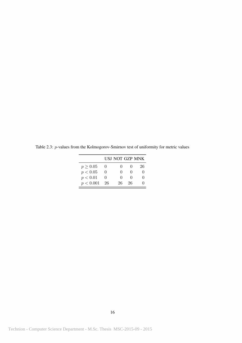
Table 2.3: p-values from the Kolmogorov-Smirnov test of uniformity for metric values

USJ NOT GZP MNK

p ≥ 0.05 0 0 0 26p < 0.05 0 0 0 0p < 0.01 0 0 0 0p < 0.001 26 26 26 0

16


Chapter 3

Structured Gotos are (Slightly)Harmful

3.1 Initial Hypotheses

Dijkstra’s strident advocacy for the elimination of goto [10] has long-since been accepted as

conventional wisdom among software engineers. On this basis, we conjectured that unstructured

jumps (USJ) would correlate with defects and, more generally, with other development-effort

metrics. We conjectured that this correlation could even be stronger than that of method size

in tokens (NOT) or compressed method size in bytes (GZP). We of course expected the control

metric (MNK) to show little to no correlation.

3.2 Preliminary χ2 Tests

We performed a χ2 test of independence to see the likelihood that defect Proneness is condition-

ally independent from all our code metrics, displaying the results in Table 3.1.

Under the χ2 test’s null hypothesis, defect Proneness and code metrics have no relation, and

defect-prone methods should thus exhibit the same distributions of metric values as non-defective

methods. If we reject the null hypothesis, the alternative is that defective and nondefective

methods have significantly different distributions of metric values.

The table shows the following. Defect Proneness in all corpora presents a very strong

significant relationship with USJ. 22 showed very strong significance (and 1 regular significance)

against NOT, and 24 showed very strong significance (and 1 regular significance) against GZP.

As expected for p < 0.05, two out of the 26 corpora (7.7%) showed a significant relationship

with the random MNK metric. Most of the relationships we found were extremely strong, with

p < 0.001 being the mode likelihood of the null hypothesis.

17


3.3 Predictive power of code metrics

Kendall’s τb is a rank-correlation coefficient that measures the similarity of ordering between two

random variables. In paired samples of the form (xi, yi) from two random variables, samples

are concordant when xi ≤ xj and yi ≤ yj , discordant when xi ≤ xj but yj ≤ yi, and neither

otherwise. The tau coefficient is then defined by subtracting the number of discordant pairs

from the number of concordant pairs and dividing by a normalization constant to bring the result

between -1 and +1. The tau coefficient’s distribution has an expected-value of 0, and becomes

approximately normal (with mean of 0, again) with large sample sizes. Since our sample size

is in the thousands, we employed the normal approximation to perform a hypothesis test for

significant deviation from the null hypothesis of no rank-correlation.

Each of our τb tables lists corpora as its rows and metrics as its columns, giving per-metric

mean τb values at the bottom to tell us how well the metric predicted the matching measurement

(of code defects or development effort) on average. The values range from -1.0 for deterministic

anticorrelation to 1.0 for deterministic correlation.

3.3.1 Metrics predicting Defects

Table 3.2 and Table 3.3 show the results of measuring Kendall’s τb between metrics and Defects

under no normalization, size-normalization, and rank-normalization.

USJ best predicted Defects, but only very slightly compared to NOT. The vast majority

of the correlations were statistically significant, with MNK showing a significant (p < 0.05)

correlation only once among all 26 corpora.

Size-normalizing the metrics added information to their values from NOT, which explains

their all maintaining or even gaining statistical significance, even MNK. USJ maintains a no-

ticeable mean correlation with Defects, while GZP and MNK had their information content

dominated by that of NOT and became anticorrelated with Defects. Rank-normalizing the

correlations between metrics and Defects had a similar but stronger effect, with only USJ

maintaining a positive 0.0136 correlation.

3.3.2 Metrics predicting Churn

Table 3.4 and Table 3.5 show the results of measuring Kendall’s τb between metrics and Churn

under no normalization, size-normalization, and rank-normalization.

GZP most strongly predicted Churn , followed closely by NOT and then, with a lower mean

τb by nearly 0.10, USJ. All correlations were significant in all corpora, except for those with

MNK, for which p < 0.05 was obtained only twice in 26 corpora.

Size-normalization once again resulted in USJ being the only metric to hold on to positive

correlation rather than becoming dominated by NOT’s information content: USJ had a positive

and substantial mean taub after size normalization while all other metrics anticorrelated. Statis-

tical significances were again maintained, and added to MNK by the information content of the

normalization.

18


Rank-normalizing metrics and then measuring their correlation to Churn found all rank-

normalized metrics to be uninformative due to being dominated by the NOT ranks, losing positive

correlation. GZP showed the least anticorrelation.

3.3.3 Metrics predicting Maintenance

Table 3.6 and Table 3.7 show the results of measuring Kendall’s τb between metrics and

Maintenance under no normalization, size-normalization, and rank-normalization.

GZP showed the highest average correlation with Maintenance , followed by NOT and USJ.

USJ’s correlations were statistically significant less often than those of NOT and GZP. None of

the metrics had a larger τb value with Maintenance than 0.10.

Size-normalization again found GZP and MNK to anticorrelate with Maintenance , although

USJ merely lost some statistical significances while maintaining a low but positive correlation.

Rank-normalization caused USJ and MNK to anticorrelate with Maintenance, while GZP

merely lost significance but maintained a barely positive mean correlation.

3.3.4 Cross-Correlation of Metrics

Taking correlation between the metrics and each-other showed that most real metrics correlate

with each-other (Table 3.8), although USJ showed a weak-enough correlation with NOT and

GZP to indicate that it contains independent information about code. After size-normalization

these correlations still exist, albeit as anticorrelations (Table 3.8). After rank-normalization a

τb = 0.0672 correlation existed between USJ and GZP, while a τb = 0.3624 correlation held

between USJ and MNK (Table 3.8); this indicates that most information in rank-normalized

metrics derives from NOT.

Table 3.9 shows the differences in metric percentiles between defective methods and nonde-

fective methods across projects, giving averages over projects and metrics.

3.3.5 Difference of Means between Defective and Nondefective Methods

When measuring whether methods with nonzero Defects have higher metric values than methods

with zero Defects, we found GZP to show the largest difference (8.04 percentiles difference),

NOT the second-largest (7.77 percentiles difference), and USJ the smallest (3.46 percentiles

difference) (Table 3.9).

3.4 Findings

We observed strongly significant evidence in the χ2 test for a relationship between unstructured

jumps and the presence or absence (but not quantity) of Defects, but also for a relationship

between program size and compressed size and defects (Section 3.2). However, very large

sample sizes yield very high power in statistical hypothesis tests; this can lead to very small

19


effects becoming significant. The randomized MNK metric having achieved significance twice in

the χ2 test shows that this may have occurred in our experiment.

In Subsection 3.3.1 we measured the ability of metrics to predict Defects . Our correlation

measurements found USJ to be, slightly but significantly, the strongest predictor of Defects,

to lose only 0.0279 points of correlation under size-normalization while all other metrics gain

anticorrelation, and to maintain a τb = 0.0136 correlation under rank-normalization when all

other metrics gain anticorrelation.

Although corpora G, M, P, V, and W showed outlying (τb < 0.0500) correlations with NOT

and GZP, these corpora still showed their strongest Defects-correlation with USJ; P, V, and W

still showed τb ≥ 0.0500 with USJ. M, the only corpus to fail a significance test for correlation

between NOT and Defects, still rejected the null hypothesis with p < 0.01 when testing the

link between USJ and Defects . Likewise, M and V showed significant anticorrelation between

compressed program size and Defects , but still both showed significance between Defects and

USJ. As in all other corpora, the links between USJ and Defects in these corpora are almost

entirely maintained under size-normalization and appear to increase under rank-normalization.

Overall, it appears that USJ provides slight but significant power to predict Defects, not

only independently from NOT but even when NOT cannot predict very well itself.

When we measured in terms of Churn instead of Defects in Subsection 3.3.2, we find that

GZP becomes the best predictor, while under size-normalization USJ loses only 0.0460 points

of its correlation. Under rank-normalization, GZP returns to being the best predictor, with only

-.0003 anticorrelation. A priori, since Churn measures the cumulative number of lines of code

that were changed in a method across its lifetime, we expect it to correlate more strongly with

size metrics such as NOT and GZP rather than specific programming constructs like USJ. The

performance of USJ under size-normalization does provide weak evidence in its favor as a

predictor, however.

Measuring in terms of Maintenance (changed lines in code with nonzero Defects) would

be expected to again correlate closely with program size or compressed size, and so it did in

Subsection 3.3.3. GZP showed the most predictive power against Maintenance prior to any

normalizations, and again kept its correlation under rank-normalization.

P and S were outlier corpora; in the former there were no significant correlations, and in the

latter USJ showed the largest correlation with Maintenance and the only statistical significance.

P showed a significant positive correlation between GZP and Maintenance after the size and rank

normalizations, and S showed a link between USJ and Maintenance after size-normalization

while linking GZP and Maintenance after rank-normalization.

In contrast to GZP, USJ kept its positive correlations with Maintenance under size-normalization,

losing only 0.0092 points of correlation. In some cases, it even maintained a statistically signifi-

cant positive correlation with Maintenance under rank-normalization.

In Subsection 3.3.5 we found that methods possessing nonzero Defects tend to have higher

average metric-value percentiles than those with zero Defects. However, this difference is

smaller in USJ than in NOT and GZP.

Overall, it appears that goto may deserve to be “considered harmful”. If this conclusion

20


appears trivially intuitive, we still benefit from having empirical evidence in its favor. However,

our results are not entirely trivial: instead of finding that goto is very strongly harmful (as

Dijkstra held) or not harmful at all (as Knuth and others held), we find that it is weakly harmful,

but with great statistical significance. We also found, more often than not, that rather than NOT

having the greatest predictive power, either USJ (unstructured jumps) or GZP (compressed size)

did.

21


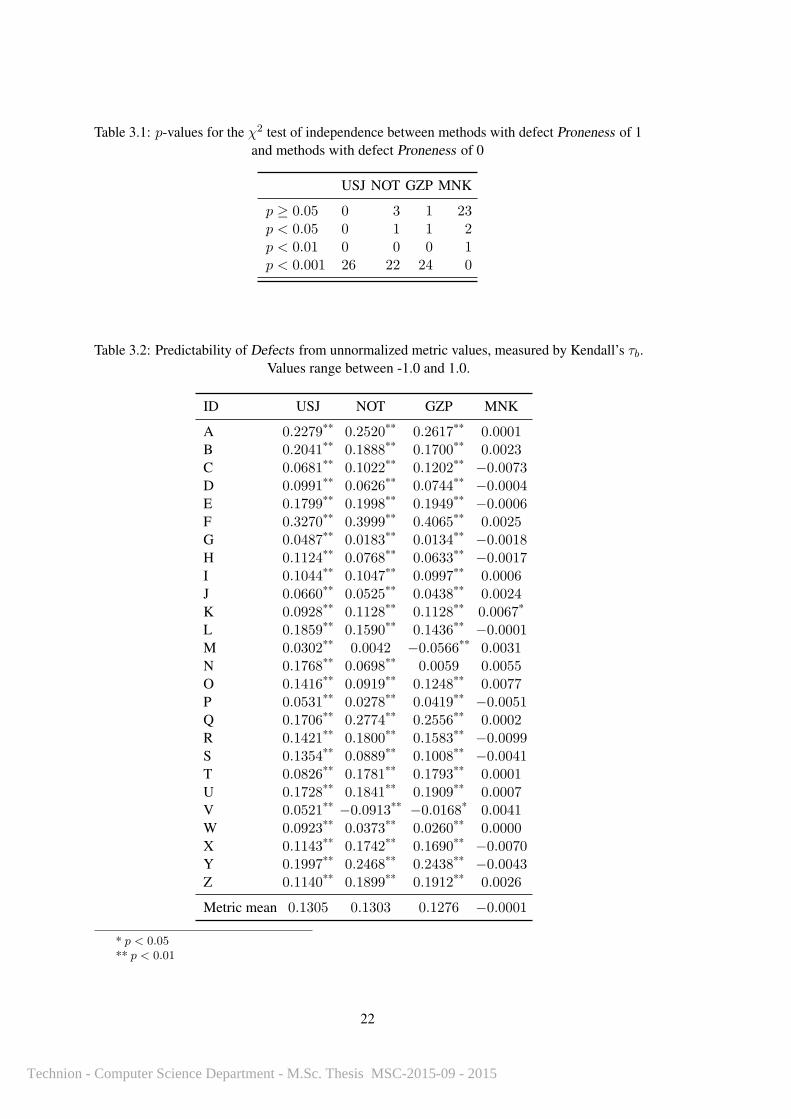
Table 3.1: p-values for the χ2 test of independence between methods with defect Proneness of 1and methods with defect Proneness of 0

USJ NOT GZP MNK

p ≥ 0.05 0 3 1 23p < 0.05 0 1 1 2p < 0.01 0 0 0 1p < 0.001 26 22 24 0

Table 3.2: Predictability of Defects from unnormalized metric values, measured by Kendall’s τb.Values range between -1.0 and 1.0.

ID USJ NOT GZP MNK

A 0.2279** 0.2520** 0.2617** 0.0001B 0.2041** 0.1888** 0.1700** 0.0023C 0.0681** 0.1022** 0.1202** −0.0073D 0.0991** 0.0626** 0.0744** −0.0004E 0.1799** 0.1998** 0.1949** −0.0006F 0.3270** 0.3999** 0.4065** 0.0025G 0.0487** 0.0183** 0.0134** −0.0018H 0.1124** 0.0768** 0.0633** −0.0017I 0.1044** 0.1047** 0.0997** 0.0006J 0.0660** 0.0525** 0.0438** 0.0024K 0.0928** 0.1128** 0.1128** 0.0067*

L 0.1859** 0.1590** 0.1436** −0.0001M 0.0302** 0.0042 −0.0566** 0.0031N 0.1768** 0.0698** 0.0059 0.0055O 0.1416** 0.0919** 0.1248** 0.0077P 0.0531** 0.0278** 0.0419** −0.0051Q 0.1706** 0.2774** 0.2556** 0.0002R 0.1421** 0.1800** 0.1583** −0.0099S 0.1354** 0.0889** 0.1008** −0.0041T 0.0826** 0.1781** 0.1793** 0.0001U 0.1728** 0.1841** 0.1909** 0.0007V 0.0521** −0.0913** −0.0168* 0.0041W 0.0923** 0.0373** 0.0260** 0.0000X 0.1143** 0.1742** 0.1690** −0.0070Y 0.1997** 0.2468** 0.2438** −0.0043Z 0.1140** 0.1899** 0.1912** 0.0026

Metric mean 0.1305 0.1303 0.1276 −0.0001

* p < 0.05** p < 0.01

22


Table 3.3: Predictability of Defects from size-normalized and rank-normalized metric values,measured by Kendall’s τb. Values range between -1.0 and 1.0.

Size USJ GZP MNK

A 0.16** −0.19** −0.20**

B 0.17** −0.20** −0.16**

C 0.05** −0.06** −0.08**

D 0.08** −0.04** −0.06**

E 0.16** −0.18** −0.16**

F 0.16** −0.35** −0.32**

G 0.05** −0.02** −0.02**

H 0.10** −0.06** −0.06**

I 0.09** −0.09** −0.08**

J 0.05** −0.06** −0.04**

K 0.07** −0.08** −0.09**

L 0.18** −0.14** −0.13**

M 0.03** −0.11** 0.00N 0.17** −0.17** −0.05**

O 0.13** −0.02* −0.07**

P 0.05** 0.00 −0.02*

Q 0.11** −0.27** −0.23**

R 0.08** −0.18** −0.15**

S 0.11** −0.05** −0.07**

T 0.04** −0.13** −0.14**

U 0.15** −0.11** −0.14**

V 0.05** 0.10** 0.07**

W 0.09** −0.04** −0.03**

X 0.09** −0.14** −0.14**

Y 0.16** −0.21** −0.20**

Z 0.09** −0.15** −0.15**

Metric mean 0.10 −0.11 −0.10

Rank USJ GZP MNK

A 0.04** 0.06** −0.15**

B −0.04** −0.06** −0.11**

C −0.02 0.01 −0.07**

D 0.07** 0.02** −0.03**

E 0.00 0.00 −0.13**

F −0.13** 0.05** −0.26**

G 0.09** −0.03** 0.00H 0.04** −0.04** −0.05**

I 0.06** −0.02** −0.07**

J 0.02** −0.02** −0.03**

K 0.00 0.01 −0.06**

L 0.05** −0.02 −0.10**

M 0.10** −0.19** −0.01**

N 0.02** −0.18** −0.04**

O 0.07** 0.05** −0.05**

P 0.15** 0.03** −0.02*

Q −0.22** −0.02** −0.16**

R −0.02* −0.06** −0.11**

S 0.03** 0.01 −0.06**

T −0.06** 0.05** −0.11**

U 0.07** 0.02** −0.12**

V 0.11** 0.02* 0.06**

W 0.15** −0.04** −0.03**

X 0.04** 0.01 −0.11**

Y −0.11** −0.01* −0.16**

Z −0.10** 0.03** −0.12**

Metric mean 0.02 −0.01 −0.08

a* p < 0.05b** p < 0.01

23


Table 3.4: Predictability of Churn from unnormalized metric values, measured by Kendall’s τb.Values range between -1.0 and 1.0.

ID USJ NOT GZP MNK

A 0.3299** 0.4073** 0.4223** −0.0017B 0.2398** 0.2266** 0.1937** −0.0032C 0.1801** 0.3026** 0.3033** −0.0160D 0.1287** 0.1230** 0.1300** −0.0069E 0.2111** 0.3241** 0.3124** 0.0012F 0.4153** 0.5341** 0.5350** −0.0035G 0.1734** 0.1377** 0.1452** −0.0062H 0.2184** 0.3960** 0.3966** −0.0033I 0.2160** 0.3290** 0.3281** −0.0007J 0.1244** 0.1986** 0.1925** 0.0033K 0.2100** 0.3588** 0.3557** −0.0027L 0.3052** 0.4437** 0.4417** 0.0065M 0.1451** 0.2038** 0.1452** 0.0001N 0.1786** 0.1941** 0.1439** 0.0035O 0.2215** 0.3948** 0.4396** −0.0044P 0.1996** 0.3031** 0.3239** −0.0175*

Q 0.3433** 0.5422** 0.5234** 0.0054R 0.3936** 0.5559** 0.5453** −0.0084S 0.2614** 0.3632** 0.3723** −0.0139*

T 0.2002** 0.2710** 0.2711** −0.0008U 0.3282** 0.3947** 0.4049** 0.0022V 0.0738** 0.1583** 0.3188** −0.0012W 0.2402** 0.2959** 0.3260** −0.0039X 0.2196** 0.3165** 0.3287** 0.0021Y 0.3039** 0.5038** 0.5002** −0.0050Z 0.2446** 0.3741** 0.3656** 0.0025

Metric mean 0.2348 0.3328 0.3371 −0.0028

* p < 0.05** p < 0.01

24


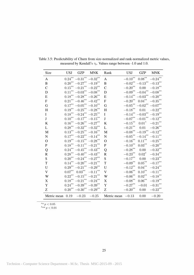
Table 3.5: Predictability of Churn from size-normalized and rank-normalized metric values,measured by Kendall’s τb. Values range between -1.0 and 1.0.

Size USJ GZP MNK

A 0.24** −0.31** −0.32**

B 0.20** −0.27** −0.19**

C 0.15** −0.21** −0.22**

D 0.11** −0.03** −0.08**

E 0.18** −0.28** −0.26**

F 0.21** −0.46** −0.42**

G 0.17** −0.05** −0.10**

H 0.19** −0.25** −0.28**

I 0.18** −0.24** −0.25**

J 0.10** −0.17** −0.15**

K 0.16** −0.26** −0.27**

L 0.28** −0.32** −0.32**

M 0.13** −0.25** −0.16**

N 0.17** −0.22** −0.14**

O 0.19** −0.15** −0.28**

P 0.18** −0.11** −0.21**

Q 0.24** −0.45** −0.43**

R 0.28** −0.40** −0.43**

S 0.20** −0.24** −0.27**

T 0.14** −0.20** −0.21**

U 0.29** −0.21** −0.29**

V 0.07** 0.03** −0.11**

W 0.22** −0.15** −0.21**

X 0.18** −0.21** −0.24**

Y 0.24** −0.39** −0.39**

Z 0.20** −0.30** −0.29**

Metric mean 0.19 −0.23 −0.25

Rank USJ GZP MNK

A −0.10** 0.08** −0.24**

B −0.02** −0.13** −0.13**

C −0.20** 0.00 −0.18**

D −0.09** −0.04** −0.08**

E −0.14** −0.03** −0.20**

F −0.20** 0.04** −0.35**

G −0.05** −0.02** −0.07**

H −0.18** 0.01 −0.22**

I −0.14** −0.03** −0.19**

J −0.07** −0.01** −0.12**

K −0.15** 0.01* −0.21**

L −0.21** 0.01 −0.26**

M −0.08** −0.19** −0.12**

N −0.05** −0.14** −0.11**

O −0.16** 0.11** −0.25**

P −0.10** 0.03** −0.20**

Q −0.28** 0.00 −0.32**

R −0.23** 0.02* −0.34**

S −0.17** 0.00 −0.23**

T −0.09** 0.05** −0.17**

U −0.12** 0.04** −0.24**

V −0.06** 0.10** −0.11**

W −0.06** 0.02** −0.18**

X −0.08** 0.06** −0.19**

Y −0.27** −0.01 −0.31**

Z −0.20** 0.00 −0.22**

Metric mean −0.13 0.00 −0.20

a* p < 0.05b** p < 0.01

25


Table 3.6: Predictability of Maintenance from unnormalized metric values, measured byKendall’s τb. Values range between -1.0 and 1.0.

ID USJ NOT GZP MNK

A 0.0750** 0.1048** 0.1125** 0.0002B 0.0780** 0.0886** 0.1050** 0.0007C 0.0081 0.0335** 0.0399** 0.0110D 0.0774** 0.0619** 0.0571** −0.0009E 0.0502** 0.0639** 0.0653** 0.0071*

F 0.0843** 0.1036** 0.1027** 0.0049G 0.0071 0.0802** 0.0800** 0.0065H 0.0457** 0.0794** 0.0722** 0.0081I 0.0266** 0.0631** 0.0656** −0.0002J 0.0784** 0.0993** 0.0935** 0.0037K 0.0355** 0.0701** 0.0803** 0.0003L 0.0745** 0.0828** 0.0771** −0.0076M 0.0247** 0.0396** 0.0379** 0.0027N 0.0344** 0.0484** 0.0449** 0.0066*

O 0.1052** 0.0913** 0.0997** −0.0012P 0.0141 −0.0105 0.0012 −0.0101Q 0.0549** 0.0590** 0.0530** −0.0101R 0.0554** 0.0437** 0.0340** −0.0131S 0.0226* 0.0050 0.0099 0.0080T 0.0363** 0.0802** 0.0730** −0.0102*

U 0.0092 0.0419** 0.0524** 0.0073V −0.0023 0.0070 0.0342** 0.0181*

W 0.0387** 0.0201** 0.0085** −0.0032X 0.0394** 0.1212** 0.1154** −0.0003Y 0.0319** 0.0483** 0.0573** −0.0067Z 0.0334** 0.0630** 0.0673** −0.0031

Metric mean 0.0438 0.0611 0.0631 0.0007

* p < 0.05** p < 0.01

26


Table 3.7: Predictability of Maintenance from size-normalized and rank-normalized metricvalues, measured by Kendall’s τb. Values range between -1.0 and 1.0.

Size USJ GZP MNK

A 0.05** −0.07** −0.08**

B 0.06** −0.04** −0.07**

C 0.00 −0.01 −0.02D 0.07** −0.05** −0.05**

E 0.05** −0.05** −0.05**

F 0.04** −0.09** −0.08**

G 0.00 −0.04** −0.05**

H 0.04** −0.06** −0.06**

I 0.02** −0.04** −0.05**

J 0.07** −0.09** −0.08**

K 0.03** −0.03** −0.06**

L 0.07** −0.07** −0.06**

M 0.02** −0.01** −0.02**

N 0.03** −0.04** −0.03**

O 0.09** −0.04** −0.07**

P 0.01 0.03** 0.00Q 0.04** −0.06** −0.05**

R 0.04** −0.06** −0.04**

S 0.02* 0.01 0.01T 0.02** −0.07** −0.07**

U 0.00 0.00 −0.03**

V 0.00 0.02** 0.01W 0.04** −0.03** −0.02**

X 0.02* −0.11** −0.10**

Y 0.03** −0.02** −0.04**

Z 0.02** −0.04** −0.05**

Metric mean 0.03 −0.04 −0.05

Rank USJ GZP MNK

A 0.04** 0.02** −0.06**

B −0.07** 0.07** −0.05**

C −0.03* 0.01 −0.02D 0.01* 0.00 −0.03**

E 0.00 0.01** −0.04**

F −0.04** 0.00 −0.07**

G −0.05** 0.01* −0.04**

H −0.01 −0.01 −0.05**

I 0.01** 0.01** −0.04**

J −0.06** −0.01 −0.06**

K −0.02** 0.03** −0.04**

L 0.00 0.00 −0.05**

M 0.00 0.00 −0.03**

N −0.08** −0.01 −0.03**

O −0.01 0.04** −0.06**

P 0.08** 0.03** 0.00Q −0.11** 0.01 −0.04**

R −0.01 −0.01 −0.02*

S −0.01 0.02** 0.01T −0.02** 0.01 −0.05**

U 0.05** 0.02** −0.03**

V 0.02* 0.02* 0.00W 0.07** −0.03** −0.01**

X −0.04** 0.00 −0.07**

Y −0.02** 0.03** −0.04**

Z −0.05** 0.02** −0.04**

Metric mean −0.01 0.01 −0.04

a* p < 0.05b** p < 0.01

Table 3.8: Predictability of unnormalized, size-normalized, and rank-normalized metric valuesfrom each-other (from left to right), measured by Kendall’s τb. Values range from -1.0 to 1.0.

USJ NOT GZP MNK

USJ 1.00** 0.38** 0.36** 0.00NOT 0.38** 1.00** 0.79** 0.00GZP 0.36** 0.79** 1.00** 0.00MNK 0.00 0.00 0.00 1.00**

USJ GZP MNK

USJ 1.00** −0.25** −0.25**

GZP −0.25** 1.00** 0.44**

MNK −0.25** 0.44** 1.00**

USJ GZP MNK

USJ 1.00** 0.06** 0.35**

GZP 0.06** 1.00** 0.04**

MNK 0.35** 0.04** 1.00**

* p < 0.05** p < 0.01

27


Table 3.9: Defective methods have a mean percentile metric-value several percentage pointshigher than that of non-defective methods.

Metric A B C D E F G H I J K L M N O P Q R S T U V W X Y Z MeanMedianMinMax

USJ 0 7 0 18 6 6 0 2 4 4 5 4 6 2 6 0 3 2 1 2 0 0 3 2 1 6 3.46 2.5 0 18NOT 1 11 4 30 13 9 14 9 8 8 17 8 9 8 10−1 4 1 0 9 5 0 2 12 3 8 7.77 8 −1 30GZP 2 13 5 29 13 9 14 8 8 8 19 7 9 7 11 0 4 0 0 8 6 4 1 11 4 9 8.04 8 0 29MNK −1 0 0 2 0 1 0 0 0 0 0 0 0 0 0 0 0 0 0−1 0 1 0 0 1 0 0.12 0 −1 2

Mean 0 7 2 19 8 6 7 4 5 5 10 4 6 4 6 0 2 0 0 4 2 1 1 6 2 5 4 4 0 19Median 0 9 2 23 9 7 7 5 6 6 11 5 7 4 8 0 3 0 0 5 2 0 1 6 2 7 5 5 0 23Min −1 0 0 2 0 1 0 0 0 0 0 0 0 0 0−1 0 0 0−1 0 0 0 0 1 0 0 0 −1 2Max 2 13 5 30 13 9 14 9 8 8 19 8 9 8 11 0 4 2 1 9 6 4 3 12 4 9 8 8 0 30

28


Chapter 4

The Rediscovery of the Bug-DensityParadox

A hypothesis is sometimes advanced for why shorter code should be preferred: that all pro-

grammers produce some fixed number of bugs in any fixed-size unit of code they write. It

is thus reasoned that writing longer code creates more places for bugs to slip in undetected.

Whether this occurs independently of the program’s complexity (measured by any means) does

not appear to have been tested in the literature, nor the implied hypothesis that the likelihood

of a function or method containing a bug should rise linearly or almost linearly with its length

before asymptotically converging to unity.

Hence the usage of size metrics to predict defects, some of the most common and widely-

used of all software metrics. What, however, do they actually tell their users about defect

proneness, and in what ranges of values? Which size metrics are better at predicting defect

proneness?

4.1 Prior Expectations

Consider a method with n tokens (the smallest atomic unit of program source code as distinct

from raw text) and a uniform probability p that each token of code has a defect in it, with the

defect proneness of any two tokens being conditionally independent. The cumulative probability

that any such method has a defect in it can then be expressed simply as:

P (defect|n, p) = 1− (1− p)n (4.1)

As p becomes small:

P (defect|n, p) = fp(n) = 1− e−np (4.2)

The function given in Equation 4.2 is parameterized over p and, for any given value, rises

steeply before smoothing out into an asymptote. Varying p to higher values leads to a steeper

rise and an earlier asymptote, while reducing the value of p leads to a shallower rise and later

29


asymptote. In fact, where p is very small, the shallowly rising portion of the function can even

appear linear, though it will level off into an asymptote eventually.

0

0.2

0.4

0.6

0.8

1

0 500 1000 1500

Cum

ulat

ive

defe

ctpr

obab

ility

Method size (tokens)

Defect proneness for p = 0.003

P (n)np

Figure 4.1: In a model where each token in a method has an independent chance of containing a

defect, the cumulative probability of the method as a whole containing a defect eventually rises

to unity.

The naıve hypothesis of defect occurrence given above also suggests that defects cluster

with an even density in methods of all sizes, with new defects occurring at some fixed rate

as method length increases. Since defect density at some method length n is defined by the

number of metric-units (for example, the metric units for NOT are tokens, and those for GZP

are bytes) containing defects in a method n units long, defect density has been measured as

Defective lines of code per revision/n.

Since Maintenance, both within and across revisions, is expected to rise with the length

of the method, the naıve hypothesis predicts that defect density should appear uniform across

actual method sizes.

Figure 4.1 shows an example of how a constant per-token bug probability ought to raise

the cumulative probability of a defect as method size grows, with an example probability of

p = 0.0030.

4.2 Related Work

Fenton and Neil [12]’s comprehensive survey on the use of metrics in software engineering

argued (among other things) that size is not necessarily the single most important quality

30


indicator. Still, further studies by El Emam, Melo, and Machado [11] and Zhou, Leung, and

Xu [34] showed that size strongly confounds the use of other metrics, and others such as

Subramanyam and Krishnan [33] and Benlarbi, El Emam, and Goel [6] have required great

efforts to eliminate this effect.

Of course, the naıve hypothesis, being naıve, has been examined before, although at the

level of modules rather than individual methods. Basili and Perricone [5] measured the quantity

of lines of code in a module, in contrast to our tokens and compressed bytes in a method, and

found that defect density declined as module size increased; this was later corroborated by Shen,

Yu, Thebaut, and Paulsen [28] showing that the decline comes to an asymptote. Later work by

Hatton [14] showed that medium-sized modules have a lower defect density than either small

or large modules, whereas we have found that defect density across tokens is higher in the

relatively smallest and largest methods – our data shows only a noisy, gradual decline of defect

density when measured in terms of absolute size rather than relative.

Malaiya and Denton [21] fitted an asymptotic model to the previous studies’ data and found

that defect density increased from its low point after an optimal module size; they gave a

parametric model for finding this optimal size. We do not have a parametric model, and found a

trend of lower defect density near the median of method sizes rather than at any specific absolute

size.

4.3 Densities Plotted and Correlations Measured

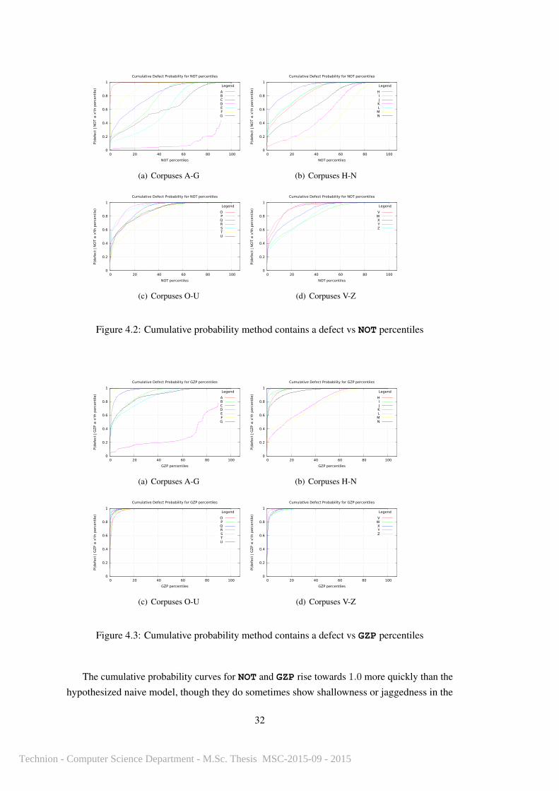
4.3.1 Cumulative Defect Likelihood functions

In order to test whether real software corpora conformed to our naive hypothesis, Figure 4.2

and Figure 4.3 show the per-method cumulative distribution functions for defect Proneness,

conditioned on size metric values.

31


0

0.2

0.4

0.6

0.8

1

0 20 40 60 80 100

P(d

efe

ct |

NO

T ≤

x't

h p

erc

enti

le)

NOT percentiles

Cumulative Defect Probability for NOT percentiles

Legend

ABCDEFG

(a) Corpuses A-G

0

0.2

0.4

0.6

0.8

1

0 20 40 60 80 100

P(d

efe

ct |

NO

T ≤

x't

h p

erc

enti

le)

NOT percentiles


Legend

HIJ

KLMN

(b) Corpuses H-N

0

0.2

0.4

0.6

0.8

1

0 20 40 60 80 100

P(d

efe

ct |

NO

T ≤

x't

h p

erc

enti

le)

NOT percentiles


Legend

OPQRSTU

(c) Corpuses O-U

0

0.2

0.4

0.6

0.8

1

0 20 40 60 80 100

P(d

efe

ct |

NO

T ≤

x't

h p

erc

enti

le)

NOT percentiles


Legend

VWXYZ

(d) Corpuses V-Z

Figure 4.2: Cumulative probability method contains a defect vs NOT percentiles

0

0.2

0.4

0.6

0.8

1

0 20 40 60 80 100

P(d

efe

ct |

GZ

P ≤

x't

h p

erc

enti

le)

GZP percentiles

Cumulative Defect Probability for GZP percentiles

Legend

ABCDEFG

(a) Corpuses A-G

0

0.2

0.4

0.6

0.8

1

0 20 40 60 80 100

P(d

efe

ct |

GZ

P ≤

x't

h p

erc

enti

le)

GZP percentiles


Legend

HIJ

KLMN

(b) Corpuses H-N

0

0.2

0.4

0.6

0.8

1

0 20 40 60 80 100

P(d

efe

ct |

GZ

P ≤

x't

h p

erc

enti

le)

GZP percentiles


Legend

OPQRSTU

(c) Corpuses O-U

0

0.2

0.4

0.6

0.8

1

0 20 40 60 80 100

P(d

efe

ct |

GZ

P ≤

x't

h p

erc

enti

le)

GZP percentiles


Legend

VWXYZ

(d) Corpuses V-Z

Figure 4.3: Cumulative probability method contains a defect vs GZP percentiles

The cumulative probability curves for NOT and GZP rise towards 1.0 more quickly than the

hypothesized naive model, though they do sometimes show shallowness or jaggedness in the

32


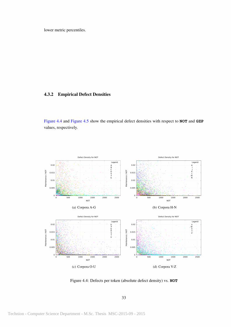
lower metric percentiles.

4.3.2 Empirical Defect Densities

Figure 4.4 and Figure 4.5 show the empirical defect densities with respect to NOT and GZP

values, respectively.

0

0.005

0.01

0.015

0.02

0 500 1000 1500 2000 2500

Main

tenance

/ N

OT

NOT

Defect Density for NOT

Legend

ABCDEFG

(a) Corpora A-G

0

0.005

0.01

0.015

0.02

0 500 1000 1500 2000 2500

Main

tenance

/ N

OT

NOT


Legend

HIJ

KLMN

(b) Corpora H-N

0

0.005

0.01

0.015

0.02

0 500 1000 1500 2000 2500

Main

tenance

/ N

OT

NOT


Legend

OPQRSTU

(c) Corpora O-U

0

0.005

0.01

0.015

0.02

0 500 1000 1500 2000 2500

Main

tenance

/ N

OT

NOT


Legend

VWXYZ

(d) Corpora V-Z

Figure 4.4: Defects per token (absolute defect density) vs. NOT

33


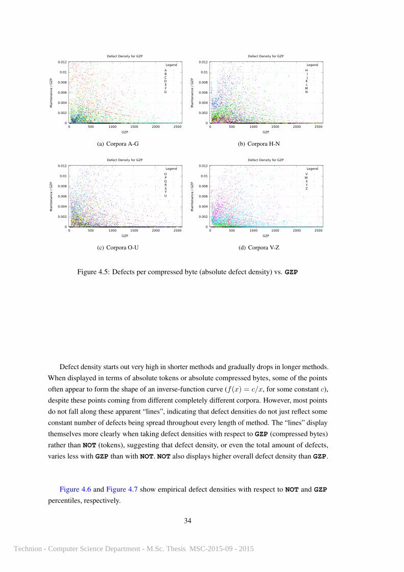
0

0.002

0.004

0.006

0.008

0.01

0.012

0 500 1000 1500 2000 2500

Main

tenance

/ G

ZP

GZP

Defect Density for GZP

Legend

ABCDEFG

(a) Corpora A-G

0

0.002

0.004

0.006

0.008

0.01

0.012

0 500 1000 1500 2000 2500

Main

tenance

/ G

ZP

GZP


Legend

HIJ

KLMN

(b) Corpora H-N

0

0.002

0.004

0.006

0.008

0.01

0.012

0 500 1000 1500 2000 2500

Main

tenance

/ G

ZP

GZP


Legend

OPQRSTU

(c) Corpora O-U

0

0.002

0.004

0.006

0.008

0.01

0.012

0 500 1000 1500 2000 2500

Main

tenance

/ G

ZP

GZP


Legend

VWXYZ

(d) Corpora V-Z

Figure 4.5: Defects per compressed byte (absolute defect density) vs. GZP

Defect density starts out very high in shorter methods and gradually drops in longer methods.

When displayed in terms of absolute tokens or absolute compressed bytes, some of the points

often appear to form the shape of an inverse-function curve (f(x) = c/x, for some constant c),

despite these points coming from different completely different corpora. However, most points

do not fall along these apparent “lines”, indicating that defect densities do not just reflect some

constant number of defects being spread throughout every length of method. The “lines” display

themselves more clearly when taking defect densities with respect to GZP (compressed bytes)

rather than NOT (tokens), suggesting that defect density, or even the total amount of defects,

varies less with GZP than with NOT. NOT also displays higher overall defect density than GZP.

Figure 4.6 and Figure 4.7 show empirical defect densities with respect to NOT and GZP

percentiles, respectively.

34


0

0.5

1

1.5

2

2.5

0 20 40 60 80 100

Main

tenance

/ N

OT p

erc

enti

les

NOT percentiles

Defect Density for NOT percentiles

Legend

ABCDEFG

(a) Corpora A-G

0

0.5

1

1.5

2

2.5

0 20 40 60 80 100

Main

tenance

/ N

OT p

erc

enti

les

NOT percentiles


Legend

HIJ

KLMN

(b) Corpora H-N

0

0.5

1

1.5

2

2.5

0 20 40 60 80 100

Main

tenance

/ N

OT p

erc

enti

les

NOT percentiles


Legend

OPQRSTU

(c) Corpora O-U

0

0.5

1

1.5

2

2.5

0 20 40 60 80 100

Main

tenance

/ N

OT p

erc

enti

les

NOT percentiles


Legend

VWXYZ

(d) Corpora V-Z

Figure 4.6: Defects per token rank percentile (relative defect density) vs. NOT percentiles

35


0

0.05

0.1

0.15

0.2

0.25

0.3

0.35

0 20 40 60 80 100

Main

tenance

/ G

ZP p

erc

enti

les

GZP percentiles

Defect Density for GZP percentiles

Legend

ABCDEFG

(a) Corpora A-G

0

0.05

0.1

0.15

0.2

0.25

0.3

0.35

0 20 40 60 80 100

Main

tenance

/ G

ZP p

erc

enti

les

GZP percentiles


Legend

HIJ

KLMN

(b) Corpora H-N

0

0.05

0.1

0.15

0.2

0.25

0.3

0.35

0 20 40 60 80 100

Main

tenance

/ G

ZP p

erc

enti

les

GZP percentiles


Legend

OPQRSTU

(c) Corpora O-U

0

0.05

0.1

0.15

0.2

0.25

0.3

0.35

0 20 40 60 80 100

Main

tenance

/ G

ZP p

erc

enti

les

GZP percentiles


Legend

VWXYZ

(d) Corpora V-Z

Figure 4.7: Defects per compressed byte rank percentile (relative defect density) vs. GZP

percentiles

We see in the graphs that when taking defect densities with respect to metric percentiles,

we found most defect density to be concentrated in the shortest and the longest methods, with

much lower densities in between. We no longer see clear trends of an apparent functional form.

We can, however, again see that NOT displays higher overall defect densities with respect to its

percentiles (rank-normalized NOT) than GZP. This suggests that relative method size may more

accurately measure defect density, with less conformity to a functional form predetermined

by the method of measurement, than absolute method size, whether measured in tokens or

compressed information content.

Table 4.1 displays the results of a Kolmogorov-Smirnov Test of Uniformity on defect

densities, used to check whether or not defect densities are significantly nonuniform.

The Kolmogorov-Smirnov test of uniformity falsified its null hypothesis in all corpora, for

both NOT and GZP, with p < 0.001, indicating that metric densities are very unlikely to be

drawn from a uniform distribution.

We compiled average empirical defect densities across size metrics and corpora into Ta-

ble 4.2, and also measured the average empirical defect densities across size-metric percentiles

and corpora, shown in Table 4.3.

NOT yielded a larger average defect density, and a larger standard deviation of defect density,

36


than GZP. While most defect-density values fell within the thousandths, Corpus A had an

unusually high defect density with respect to NOT, of 0.015.

NOT percentiles still yielded larger defect densities on average, and a larger standard

deviation of defect density, while GZP showed fewer average defects-per-percentile and less

variation. Corpora A and N stood out as having unusually high defect densities: a defects-per-

GZP-percentile of 0.143 for Corpus A, and a defects-per-NOT-percentile of 0.905 for Corpus

N.

4.3.3 Predictive Power of Metric Values for Defect Densities

As empirical data tends not to be smooth, we measured how defect density changes with size

metrics via Kendall’s τb correlation coefficient, and compiled the results into Table 4.4.

The τb correlations for defect density yielded substantial and negative correlations for both

metrics, with NOT showing stronger correlation, although correlation between GZP and defect

density varied more. In corpus D the τb for NOT was very small and statistically insignificant; in

all others it was large and achieved statistical significance with p < 0.01. All corpora yielded

statistically significant correlations with both size metrics with p < 0.01.

4.3.4 A Transformed Metric for Flat Defect Density

Based on the initial findings from these measurements, we proceeded to try to construct

a transformed size metric whose resultant defect density would not correlate significantly

with the original size metric – a metric for which defect density is (relatively) uniform. We

applied the transformation of raising a size-metric value to a given power, and varied that

power between -10.0 and +10.0, measuring the mean Kendall’s τb coefficient across projects

between the original size metric and the defect density constructed from the transformed

size metric: these measurements are displayed in Figure 4.8. We also did likewise with a

transformation of form nlogε(n), where n ranges across size-metric values: these measurements

are displayed in Figure 4.9. We used these plots to locate the points where the correlation

between the transformed metric and defect density with respect to that transformed metric

become insignificant or even zero: the points where additional units of the metric do not imply

anything about the defect density, and thus where additional units of the metric can be taken to

straightforwardly indicate the presence of additional defects.

37


Figure 4.8: Mean Kendall’s τb over all projects of defect density with respect to the metric

raised to a power ε vs ε

38


Figure 4.9: Mean Kendall’s τb value over all projects of defect density with respect to the metric

plugged into the formula nlogε(n) vs ε

Our measurement of the mean Kendall’s τb correlation between metric values and density

with respect to metric values transformed by nε produced no zeroes, with the lowest absolute

value for both metrics occurring at ε = 10.0, with τb for NOT hitting 0.10 and τb for GZP hitting

approximately 0.07. The plot of τb values for the nlogε(n) transformation yielded a zero for

NOT at approximately -5.9 (ε = −5.9 and τb = −0.006) and a zero for GZP at approximately

-6.5 (ε = −6.5 and τb = −0.006).

4.3.5 The Transformed Metric’s Predictive Power

We then checked the effectiveness of this new transformed metric by calculating Kendalls τbbetween size metrics, transformed size metrics, and the defect measurements: defect Proneness ,

Defects , Versions , Churn , and Maintenance . The results are displayed in Table 4.5, Table 4.6,

Table 4.7, Table 4.8 and Table 4.9.

We found that in all cases, the regular GZP yields a higher absolute value for τb, while the

transformed GZP yields a lower one:

1. Proneness: 0.0542 for regular GZP vs -0.0520 for transformed GZP

2. Defects: 0.1276 for regular GZP vs -0.1130 for transformed GZP

3. Churn: 0.3371 for regular GZP vs -0.3173 for transformed GZP

39


4. Versions: 0.0906 for regular GZP vs -0.0774 for transformed GZP

5. Maintenance: 0.0631 for regular GZP vs -0.0598 for transformed GZP

4.4 Discussion

Our naive hypothesis made one assumption: each token has some probability p of containing

a defect. Thus, cumulative defect probability would eventually converge to unity as method

length rises, while defect density would remain uniform across method sizes. While we did

find cumulative defect probability to quickly converge towards unity in Subsection 4.3.1, our

defect density measurements showed that defects are distributed more densely in the shortest

and longest methods in Subsection 4.3.2. Average defect densities appear higher with NOT than

with GZP, and also have nonuniform distribution with p < 0.001. Whether GZP or NOT showed

more deviation from the mean in correlation with defect density depended upon whether we

considered absolute method size or method-size percentiles.

In Subsection 4.3.3 we found that defect density within a method of fixed size falls with

increasing GZP, although less steeply than with NOT, with statistical significance but sizeable

variance across all corpora.

In contrast to previous studies of defect density, which examined module sizes, we studied

two different size metrics of individual methods. Unlike Basili and Perricone [5], we found

that defect densities rise from their low point when we examine the largest methods, rather

than showing an asymptotic relationship as in Shen et al. [28]. This fits with the findings by

Hatton [14], Malaiya and Denton [21] that there exists a module or method size with locally

minimal defect density: a “Goldilocks Principle” in which defect density concentrates in the

shortest and longest methods, while remaining very low almost everywhere in-between, as we

saw in Subsection 4.3.2. This could potentially contribute to the general decrease in defect

density as method size metrics (NOT and GZP) rise, although it remains itself unexplained. This

“Goldilocks Principle” appears to occur with respect to both the absolute size metric NOT and

with respect to the compressed-size metric GZP.

The naive hypothesis is most likely false: the probability of a defect in any given unit of

method size is very unlikely to be uniform as the size of a method rises. Not only that, but

defects grow sparser as method length in tokens (NOT) rises than as compressed size in bytes

(GZP) rises.

In Subsection 4.3.3 we found that NOT better predicts defect density than GZP, and in

Subsection 4.3.4 we showed that NOT holds more correlation to defect density than GZP when

exponentiated. We also saw that NOT, transformed by nlogε(n), attains zero correlation at a

lower absolute value of ε than GZP.

We believed that if we possessed a size metric with which defect density did not vary, it

would predict defects better than metrics with varying defect densities. Towards that purpose,

40


we proposed the following as a new size metric for defect prediction:

DenseNOT = NOT ∗ log−5.9(NOT) (4.3)

Unfortunately, our measurement of the correlation between DenseNOT found that it cannot

predict any of our defect measurements as well as the un-transformed NOTmetric, let alone better

than GZP. To the contrary, our measurements in Subsection 4.3.5 showed that untransformed

GZP is the superior predictor of most defect and development-effort measurements.

We find ourselves faced with a strange paradox: on the one hand, NOT predicts defect density

more strongly than GZP, but on the other hand, GZP predicts actual defect measurements more

strongly than both the original NOT and the density-invariant DenseNOT. The information content

of a method, taken in total, predicts its defectiveness, but marginal increases to its length in

tokens are more likely to change how densely or sparsely defects occur in the method.

41


Table 4.1: p-values for the Kolmogorov-Smirnov test of uniformity for metric densities

USJ NOT GZP MNK

p ≥ 0.05 3 0 0 0p < 0.05 1 0 0 0p < 0.01 2 0 0 0p < 0.001 20 26 26 26

Table 4.2: Mean defect densities at individual size-metric values across corpora

ID A B C D E F G Metric µ+ /− σ

NOT 1.50 · 10−2 2.42 · 10−3 3.89 · 10−3 1.28 · 10−3 8.97 · 10−4 4.08 · 10−3 2.34 · 10−3 4.27 · 10−3 +/- 4.50 · 10−3

GZP 7.36 · 10−3 1.59 · 10−3 1.43 · 10−3 5.23 · 10−4 6.62 · 10−4 2.44 · 10−3 9.62 · 10−4 2.14 · 10−3 +/- 2.22 · 10−3

ID H I J K L M N Metric µ+ /− σ

NOT 6.27 · 10−3 3.32 · 10−3 7.51 · 10−3 8.96 · 10−4 6.25 · 10−3 1.08 · 10−3 2.54 · 10−3 3.98 · 10−3 +/- 2.48 · 10−3

GZP 2.76 · 10−3 1.69 · 10−3 4.15 · 10−3 4.08 · 10−4 2.77 · 10−3 5.45 · 10−4 1.29 · 10−3 1.95 · 10−3 +/- 1.25 · 10−3

ID O P Q R S T U Metric µ+ /− σ

NOT 5.94 · 10−3 6.16 · 10−3 3.93 · 10−3 4.97 · 10−3 6.30 · 10−3 4.66 · 10−3 1.92 · 10−3 4.84 · 10−3 +/- 1.44 · 10−3

GZP 2.11 · 10−3 2.50 · 10−3 1.94 · 10−3 2.77 · 10−3 3.06 · 10−3 2.12 · 10−3 8.65 · 10−4 2.20 · 10−3 +/- 6.56 · 10−4

ID V W X Y Z Metric µ+ /− σ

NOT 4.98 · 10−3 1.16 · 10−3 6.24 · 10−3 4.80 · 10−3 2.21 · 10−3 3.88 · 10−3 +/- 1.89 · 10−3

GZP 2.05 · 10−3 5.69 · 10−4 3.18 · 10−3 2.48 · 10−3 1.30 · 10−3 1.92 · 10−3 +/- 9.09 · 10−4

* p < 0.05** p < 0.01

Table 4.3: Mean defect densities at size-metric percentiles across corpora


NOT 5.71 · 10−2 2.40 · 10−2 1.74 · 10−2 8.10 · 10−3 6.93 · 10−3 2.94 · 10−2 1.60 · 10−2 2.27 · 10−2 +/- 1.59 · 10−2

GZP 1.43 · 10−1 1.18 · 10−2 1.04 · 10−2 6.15 · 10−3 1.17 · 10−2 8.65 · 10−2 8.54 · 10−3 3.98 · 10−2 +/- 5.00 · 10−2


NOT 1.96 · 10−2 2.46 · 10−2 4.00 · 10−2 5.83 · 10−3 1.45 · 10−2 5.11 · 10−3 9.05 · 10−1 1.45 · 10−1 +/- 3.10 · 10−1

GZP 4.11 · 10−2 2.33 · 10−2 5.29 · 10−2 5.04 · 10−3 1.56 · 10−2 4.19 · 10−3 7.99 · 10−2 3.17 · 10−2 +/- 2.58 · 10−2


NOT 1.85 · 10−2 1.66 · 10−2 2.97 · 10−2 2.17 · 10−2 3.38 · 10−2 2.40 · 10−2 1.02 · 10−2 2.21 · 10−2 +/- 7.38 · 10−3

GZP 2.31 · 10−2 4.34 · 10−2 4.15 · 10−2 2.40 · 10−2 2.51 · 10−2 4.70 · 10−2 1.11 · 10−2 3.07 · 10−2 +/- 1.23 · 10−2


NOT 1.80 · 10−2 5.20 · 10−3 3.04 · 10−2 5.93 · 10−2 3.33 · 10−2 2.92 · 10−2 +/- 1.80 · 10−2

GZP 2.40 · 10−2 1.83 · 10−2 2.54 · 10−2 4.65 · 10−2 5.51 · 10−2 3.39 · 10−2 +/- 1.43 · 10−2

* p < 0.05** p < 0.01

42


Table 4.4: Predictability of defect density from size-metric values, measured by Kendall’s τb.Values range between -1.0 to 1.0.


NOT −5.19 · 10−1** −3.82 · 10−1** −4.39 · 10−1** −1.55 · 10−1** −4.21 · 10−1** −4.06 · 10−1** −4.18 · 10−1** −3.92 · 10−1 +/- 1.04 · 10−1

GZP −4.31 · 10−1** −3.32 · 10−1** −2.91 · 10−1** −7.26 · 10−2** −3.48 · 10−1** −3.35 · 10−1** −3.38 · 10−1** −3.07 · 10−1 +/- 1.03 · 10−1


NOT −3.09 · 10−1** −4.93 · 10−1** −4.79 · 10−1** −4.34 · 10−1** −3.59 · 10−1** −4.87 · 10−1** −4.35 · 10−1** −4.28 · 10−1 +/- 6.48 · 10−2

GZP −1.94 · 10−1** −4.35 · 10−1** −3.71 · 10−1** −3.37 · 10−1** −2.92 · 10−1** −4.57 · 10−1** −3.62 · 10−1** −3.50 · 10−1 +/- 8.21 · 10−2


NOT −3.03 · 10−1** −4.45 · 10−1** −4.10 · 10−1** −3.64 · 10−1** −4.63 · 10−1** −3.92 · 10−1** −4.35 · 10−1** −4.02 · 10−1 +/- 5.09 · 10−2

GZP −1.69 · 10−1** −3.77 · 10−1** −3.78 · 10−1** −3.06 · 10−1** −3.79 · 10−1** −3.27 · 10−1** −3.59 · 10−1** −3.28 · 10−1 +/- 6.99 · 10−2


NOT −3.84 · 10−1** −4.87 · 10−1** −2.59 · 10−1** −4.46 · 10−1** −4.78 · 10−1** −4.11 · 10−1 +/- 8.41 · 10−2

GZP −1.66 · 10−1** −4.38 · 10−1** −2.00 · 10−1** −3.88 · 10−1** −4.23 · 10−1** −3.23 · 10−1 +/- 1.16 · 10−1

* p < 0.05** p < 0.01

43


Table 4.5: Predictability of defect Proneness from size metrics and size metrics transformed byf(n) = nlog−5.9(n), measured by Kendall’s τb. Values range from -1.0 to 1.0.

Proneness NOT GZP f(NOT) f(GZP)

A 0.0277** 0.0316** −0.0287** −0.0430**

B 0.0851** 0.1021** −0.0809** −0.0821**

C 0.0312** 0.0374** −0.0313** −0.0392**

D 0.0619** 0.0570** −0.0609** −0.0187**

E 0.0631** 0.0645** −0.0600** −0.0447**

F 0.0886** 0.0875** −0.0783** −0.0563**

G 0.0801** 0.0794** −0.0801** −0.0767**

H 0.0737** 0.0665** −0.0723** −0.0394**

I 0.0592** 0.0617** −0.0576** −0.0413**

J 0.0927** 0.0869** −0.0924** −0.0824**

K 0.0696** 0.0799** −0.0675** −0.0443**

L 0.0716** 0.0659** −0.0719** −0.0668**

M 0.0392** 0.0376** −0.0394** −0.0378**

N 0.0473** 0.0441** −0.0470** −0.0370**

O 0.0844** 0.0909** −0.0819** −0.0406**

P −0.0161 −0.0041 0.0161 0.0056Q 0.0439** 0.0380** −0.0428** −0.0123*

R 0.0171 0.0078 −0.0130 0.0208*

S −0.0052 −0.0005 0.0051 −0.0003T 0.0775** 0.0698** −0.0767** −0.0532**

U 0.0392** 0.0493** −0.0383** −0.0241**

V 0.0060 0.0309** −0.0058 −0.0023W 0.0196** 0.0076* −0.0194** 0.0018X 0.1149** 0.1091** −0.1066** −0.0740**

Y 0.0348** 0.0447** −0.0349** −0.0409**

Z 0.0590** 0.0635** −0.0567** −0.0389**

Metric mean 0.0525 0.0542 −0.0509 −0.0372

* p < 0.05** p < 0.01

44


Table 4.6: Predictability of Defects from size metrics and size metrics transformed byf(n) = nlog−5.9(n), measured by Kendall’s τb. Values range from -1.0 to 1.0.

Defects NOT GZP f(NOT) f(GZP)

A 0.2520** 0.2617** −0.2341** −0.1086**

B 0.1888** 0.1700** −0.1841** −0.1346**

C 0.1022** 0.1202** −0.1022** −0.1058**

D 0.0626** 0.0744** −0.0597** −0.0007E 0.1998** 0.1949** −0.1923** −0.1228**

F 0.3999** 0.4065** −0.3843** −0.2858**

G 0.0183** 0.0134** −0.0176** −0.0046H 0.0768** 0.0633** −0.0718** −0.0086I 0.1047** 0.0997** −0.0936** −0.0242**

J 0.0525** 0.0438** −0.0483** −0.0244**

K 0.1128** 0.1128** −0.1046** −0.0417**

L 0.1590** 0.1436** −0.1575** −0.1116**

M 0.0042 −0.0566** −0.0035 0.0563**

N 0.0698** 0.0059 −0.0678** 0.0057O 0.0919** 0.1248** −0.0862** −0.0429**

P 0.0278** 0.0419** −0.0278** −0.0368**

Q 0.2774** 0.2556** −0.2195** −0.0311**

R 0.1800** 0.1583** −0.1584** −0.0141S 0.0889** 0.1008** −0.0875** −0.0679**

T 0.1781** 0.1793** −0.1728** −0.1256**

U 0.1841** 0.1909** −0.1636** −0.0149**

V −0.0913** −0.0168* 0.0906** 0.1153**

W 0.0373** 0.0260** −0.0368** −0.0040X 0.1742** 0.1690** −0.1588** −0.0906**

Y 0.2468** 0.2438** −0.2042** −0.0644**

Z 0.1899** 0.1912** −0.1741** −0.0707**

Metric mean 0.1303 0.1276 −0.1200 −0.0523

* p < 0.05** p < 0.01

45


Table 4.7: Predictability of Churn from size metrics and size metrics transformed byf(n) = nlog−5.9(n), measured by Kendall’s τb. Values range from -1.0 to 1.0.

Churn NOT GZP f(NOT) f(GZP)

A 0.4073** 0.4223** −0.3791** −0.2171**

B 0.2266** 0.1937** −0.2128** −0.1424**

C 0.3026** 0.3033** −0.3023** −0.2785**

D 0.1230** 0.1300** −0.1211** −0.0706**

E 0.3241** 0.3124** −0.2962** −0.1883**

F 0.5341** 0.5350** −0.5091** −0.3773**

G 0.1377** 0.1452** −0.1366** −0.1114**

H 0.3960** 0.3966** −0.3891** −0.2794**

I 0.3290** 0.3281** −0.3054** −0.1477**

J 0.1986** 0.1925** −0.1924** −0.1508**

K 0.3588** 0.3557** −0.3343** −0.1704**

L 0.4437** 0.4417** −0.4417** −0.3779**

M 0.2038** 0.1452** −0.1976** −0.1059**

N 0.1941** 0.1439** −0.1914** −0.1027**

O 0.3948** 0.4396** −0.3860** −0.2760**

P 0.3031** 0.3239** −0.3031** −0.3154**

Q 0.5422** 0.5234** −0.4763** −0.2271**

R 0.5559** 0.5453** −0.5123** −0.3042**

S 0.3632** 0.3723** −0.3593** −0.3147**

T 0.2710** 0.2711** −0.2630** −0.1905**

U 0.3947** 0.4049** −0.3693** −0.1507**

V 0.1583** 0.3188** −0.1559** −0.1250**

W 0.2959** 0.3260** −0.2929** −0.2283**

X 0.3165** 0.3287** −0.2988** −0.2155**

Y 0.5038** 0.5002** −0.4442** −0.2128**

Z 0.3741** 0.3656** −0.3543** −0.2008**

Metric mean 0.3328 0.3371 −0.3163 −0.2108

* p < 0.05** p < 0.01

46


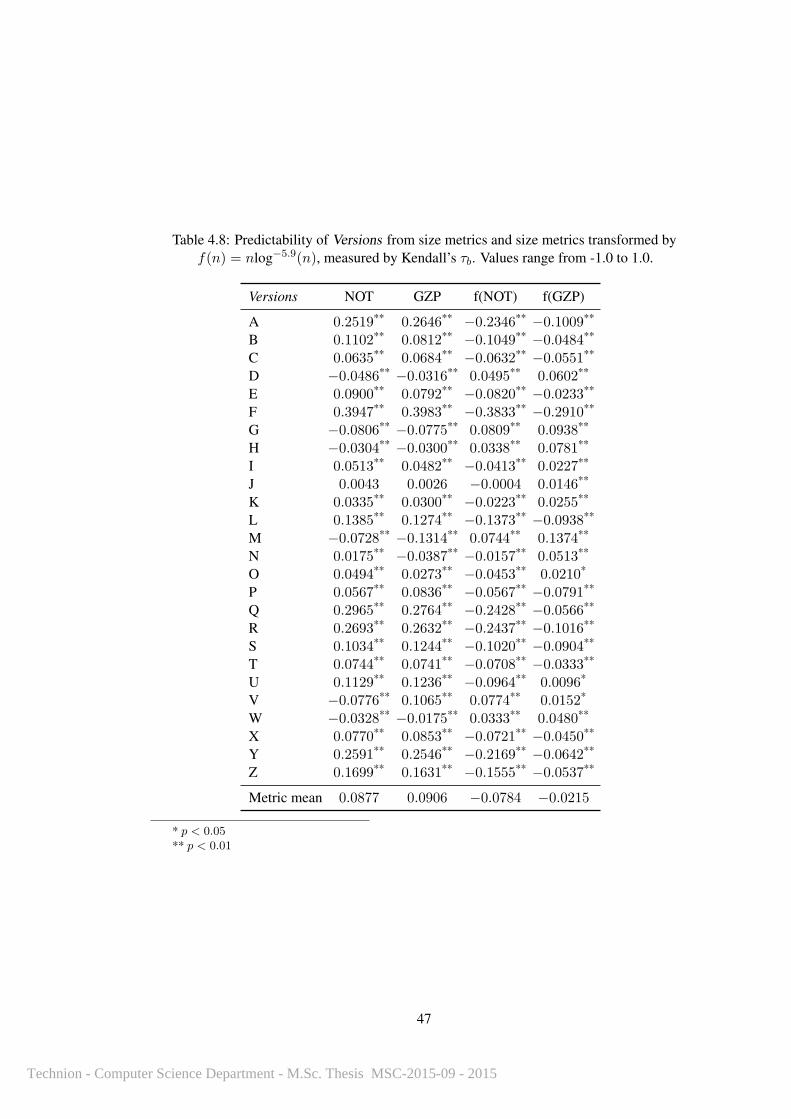
Table 4.8: Predictability of Versions from size metrics and size metrics transformed byf(n) = nlog−5.9(n), measured by Kendall’s τb. Values range from -1.0 to 1.0.

Versions NOT GZP f(NOT) f(GZP)

A 0.2519** 0.2646** −0.2346** −0.1009**

B 0.1102** 0.0812** −0.1049** −0.0484**

C 0.0635** 0.0684** −0.0632** −0.0551**

D −0.0486** −0.0316** 0.0495** 0.0602**

E 0.0900** 0.0792** −0.0820** −0.0233**

F 0.3947** 0.3983** −0.3833** −0.2910**

G −0.0806** −0.0775** 0.0809** 0.0938**

H −0.0304** −0.0300** 0.0338** 0.0781**

I 0.0513** 0.0482** −0.0413** 0.0227**

J 0.0043 0.0026 −0.0004 0.0146**

K 0.0335** 0.0300** −0.0223** 0.0255**

L 0.1385** 0.1274** −0.1373** −0.0938**

M −0.0728** −0.1314** 0.0744** 0.1374**

N 0.0175** −0.0387** −0.0157** 0.0513**

O 0.0494** 0.0273** −0.0453** 0.0210*

P 0.0567** 0.0836** −0.0567** −0.0791**

Q 0.2965** 0.2764** −0.2428** −0.0566**

R 0.2693** 0.2632** −0.2437** −0.1016**

S 0.1034** 0.1244** −0.1020** −0.0904**

T 0.0744** 0.0741** −0.0708** −0.0333**

U 0.1129** 0.1236** −0.0964** 0.0096*

V −0.0776** 0.1065** 0.0774** 0.0152*

W −0.0328** −0.0175** 0.0333** 0.0480**

X 0.0770** 0.0853** −0.0721** −0.0450**

Y 0.2591** 0.2546** −0.2169** −0.0642**

Z 0.1699** 0.1631** −0.1555** −0.0537**

Metric mean 0.0877 0.0906 −0.0784 −0.0215

* p < 0.05** p < 0.01

47


Table 4.9: Predictability of Maintenance from size metrics and size metrics transformed byf(n) = nlog−5.9(n), measured by Kendall’s τb. Values range from -1.0 to 1.0.

Maintenance NOT GZP f(NOT) f(GZP)

A 0.1048** 0.1125** −0.0988** −0.0690**

B 0.0886** 0.1050** −0.0836** −0.0825**

C 0.0335** 0.0399** −0.0335** −0.0415**

D 0.0619** 0.0571** −0.0609** −0.0186**

E 0.0639** 0.0653** −0.0605** −0.0445**

F 0.1036** 0.1027** −0.0919** −0.0637**

G 0.0802** 0.0800** −0.0803** −0.0767**

H 0.0794** 0.0722** −0.0777** −0.0416**

I 0.0631** 0.0656** −0.0608** −0.0417**

J 0.0993** 0.0935** −0.0983** −0.0853**

K 0.0701** 0.0803** −0.0678** −0.0438**

L 0.0828** 0.0771** −0.0830** −0.0752**

M 0.0396** 0.0379** −0.0397** −0.0379**

N 0.0484** 0.0449** −0.0480** −0.0373**

O 0.0913** 0.0997** −0.0882** −0.0431**

P −0.0105 0.0012 0.0105 0.0005Q 0.0590** 0.0530** −0.0552** −0.0182**

R 0.0437** 0.0340** −0.0364** 0.0056S 0.0050 0.0099 −0.0049 −0.0089T 0.0802** 0.0730** −0.0790** −0.0536**

U 0.0419** 0.0524** −0.0404** −0.0233**

V 0.0070 0.0342** −0.0068 −0.0032W 0.0201** 0.0085** −0.0199** 0.0017X 0.1212** 0.1154** −0.1110** −0.0738**

Y 0.0483** 0.0573** −0.0464** −0.0432**

Z 0.0630** 0.0673** −0.0602** −0.0397**

Metric mean 0.0611 0.0631 −0.0586 −0.0407

* p < 0.05** p < 0.01

48


Chapter 5

Conclusion and open questions

5.1 Gotos are Sometimes Somewhat Harmful

In Section 3.2 we found that USJ also achieved statistical significance in the relationship between

its values and the defect Proneness of methods most often among all the metrics. Section 3.3

presented evidence from the τb coefficients between unnormalized, size-normalized, and rank-

normalized metrics and Defects to show USJ to be a strong predictor of defect proneness, even

after accounting for the influence of absolute and relative method size. In Subsection 3.3.5 we

found that the differences in average ranks of metric values between defective and nondefective

methods are approximately five percentiles higher for NOT and GZP than for USJ.

The unstructured jumps we examined may correlate only weakly with defect proneness

because they lump together several different aspects of the code’s real semantics: noncontextual

unstructured jumps contain both ordinary short-circuit evaluation and the throw statement.

goto-like statements may be particularly unharmful in JAVA thanks to several compile-time

checks: all methods with non-void type must return a value in all their code paths, and all

possible exceptions must be declared in method signatures. Languages such as C++ [32], which

allow for the same kind of programming without performing these checks, may have more bugs

in goto-filled code than JAVA.

goto may increase defect rates by making control-flow graphs less modular (a greater

value for McCabe’s essential complexity [23]). Unusual looping constructs would then be

“considered harmful” less than employing goto or goto-like statements to make the control-

flow graph more connected as a whole, or decide which expressions (with relevant side-effects)

to evaluate at all. They could also increase defect rates by increasing the program string’s length

or descriptive complexity in ways irrelevant to the original program semantics, leaving more

locations for defects to occur by random mistake.

A priori, we did not know how much code’s length and its information content would

correlate. Empirically, in Subsection 3.3.4 we found a 0.7945 correlation coefficient (with

p < 0.01) between NOT and GZP.

49


5.2 Defects are Concentrated in Smaller Methods

What we and most previous researchers have investigated is the relationship between defects and

metrics over ordinary source code, such as length or syntactic structure. However, we believe

that engineering metrics over ordinary source code are potentially deceptive: in the real world,

after all, a programming language is considered more powerful precisely when it allows more

semantic information to be encoded in shorter code. We should thus expect that some tokens or

lines of code will be “more equal than others” in almost all real programming languages.

This conjecture is born out by the examination of defect density: defect density declines

as both NOT and GZP rise, with larger methods clearly having their defects more sparsely

distributed than shorter methods and NOT predicting defect density more strongly than GZP, as

stated in Subsection 4.3.3. Both size metrics suffer from a declining marginal power to predict

defects. However, GZP predicts Proneness , Churn , Versions , and Maintenance better than NOT,

and Subsection 4.3.4 and Subsection 4.3.5 showed that even a density-invariant transformed

NOT does strictly worse than its original.

GZP predicting our defect measurements better than NOT aligns with the speculation in

Jbara and Feitelson [15] that code comprehensibility, and thus perhaps defect proneness, comes

from the information content of code rather than from specific properties of its control-flow

graph. However, this theory would have predicted that GZP would show a consistently higher

defect density and strongly predict defect density, which Subsection 4.3.2 and Subsection 4.3.3

showed it not to do.

One way to study this counterintuitive phenomenon in-depth would be to examine software

metrics in code stored as intermediate representation (such as Java/.NET byte-code, GNU

Compiler Collection1 intermediate representation, or LLVM [20] intermediate code). Intermedi-

ate representations carry syntactic and semantic information about code structure, but with a

relatively more uniform level of such information adhering to each individual instruction.

1http://www.gnu.org/software/gcc/index.html

50


Bibliography

[1] Miltiadis Allamanis and Charles Sutton. Mining source code repositories at massive scale

using language modeling. In Proceedings of the Tenth International Workshop on Mining

Software Repositories, pages 207–216. IEEE Press, 2013.

[2] Frances E. Allen. Control flow analysis. SIGPLAN Notices, 5(7):1–19, July 1970. ISSN

0362-1340. doi: 10.1145/390013.808479. URL http://doi.acm.org/10.

1145/390013.808479.

[3] Ken Arnold and James Gosling. The JAVA Programming Language. The Java Series.

Addison-Wesley, Reading, Massachusetts, 1996. ISBN 0-201-63455-4.

[4] H. Barkmann, R. Lincke, and W. Lowe. Quantitative evaluation of software quality

metrics in open-source projects. In Advanced Information Networking and Applications

Workshops, 2009. WAINA ’09. International Conference on, pages 1067–1072, May 2009.

doi: 10.1109/WAINA.2009.190.

[5] Victor R. Basili and Barry T. Perricone. Software errors and complexity: An empirical

investigation0. Communications of the ACM, 27(1):42–52, January 1984. ISSN 0001-

0782. doi: 10.1145/69605.2085. URL http://doi.acm.org/10.1145/

69605.2085.

[6] Saida Benlarbi, Khaled El Emam, and Nishith Goel. Issues in validating object-oriented

metrics for early risk prediction. by Cistel Technology, 210, 1999.

[7] Avrim L. Blum and Pat Langley. Selection of relevant features and examples in ma-

chine learning. Artificial Intelligence, 97(1-2):245–271, December 1997. ISSN 0004-

3702. doi: 10.1016/S0004-3702(97)00063-5. URL http://dx.doi.org/

10.1016/S0004-3702(97)00063-5.

[8] Corrado Bohm and Giuseppe Jacopini. Flow diagrams, Turing machines and languages

with only two formation rules. Communications of the ACM, 9(5):366–371, May 1966.

ISSN 0001-0782. doi: 10.1145/355592.365646. URL http://doi.acm.org/

10.1145/355592.365646.

[9] Fernando Brito e Abreu, Miguel Goulao, and Rita Esteves. Toward the design quality eval-

uation of object-oriented software systems. In 5th International Conference on Software

Quality (5ICSQ), Austin, Texas, USA, pages 44–57. ASQ, 1995.

51


http://dx.doi.org/10.1145/390013.808479

http://doi.acm.org/10.1145/390013.808479

http://doi.acm.org/10.1145/390013.808479

http://dx.doi.org/10.1109/WAINA.2009.190

http://dx.doi.org/10.1145/69605.2085

http://doi.acm.org/10.1145/69605.2085

http://doi.acm.org/10.1145/69605.2085

http://dx.doi.org/10.1016/S0004-3702(97)00063-5

http://dx.doi.org/10.1016/S0004-3702(97)00063-5

http://dx.doi.org/10.1016/S0004-3702(97)00063-5

http://dx.doi.org/10.1145/355592.365646

http://doi.acm.org/10.1145/355592.365646

http://doi.acm.org/10.1145/355592.365646

[10] Edsger W. Dijkstra. Letters to the editor: GOTO statement considered harmful. Commu-

nications of the ACM, 11(3):147–148, March 1968. ISSN 0001-0782. doi: 10.1145/

362929.362947. URL http://doi.acm.org/10.1145/362929.362947.

[11] Khaled El Emam, Walcelio Melo, and Javam C Machado. The prediction of faulty classes

using object-oriented design metrics. Journal of Systems and Software, 56(1):63–75, 2001.

[12] Norman E. Fenton and Martin Neil. A critique of software defect prediction models. IEEE

Trans. Softw. Eng., 25(5):675–689, September 1999. ISSN 0098-5589. doi: 10.1109/

32.815326. URL http://dx.doi.org/10.1109/32.815326.

[13] D. Gray, D. Bowes, Neil Davey, Yi Sun, and Bruce Christianson. Software defect prediction

using static code metrics underestimates defect-proneness. In Neural Networks (IJCNN),

The 2010 International Joint Conference on, pages 1–7, July 2010. doi: 10.1109/

IJCNN.2010.5596650.

[14] Les Hatton. Reexamining the fault density-component size connection. IEEE Software, 14

(2):89–97, March 1997. ISSN 0740-7459. doi: 10.1109/52.582978. URL http:

//dx.doi.org/10.1109/52.582978.

[15] Ahmad Jbara and Dror G. Feitelson. On the effect of code regularity on comprehension. In

Proceedings of the 22nd International Conference on Program Comprehension, ICPC 2014,

pages 189–200, New York, NY, USA, 2014. ACM. ISBN 978-1-4503-2879-1. doi: 10.

1145/2597008.2597140. URL http://doi.acm.org/10.1145/2597008.

2597140.

[16] Brian W. Kernighan and Dennis M. Ritchie. The C Programming Language. Software

Series. Prentice-Hall, second edition, 1988.

[17] D. Knuth. Structured programming with GOTO statements. In Edward Nash Yourdon, ed-

itor, Classics in software engineering, pages 257–321. Yourdon Press, Upper Saddle River,

NJ, USA, 1979. ISBN 0-917072-14-6. URL http://dl.acm.org/citation.

cfm?id=1241515.1241535.

[18] Donald E. Knuth. Literate programming. Computer Journal, The, 27(2):97–111, May

1984. ISSN 0010-4620. doi: 10.1093/comjnl/27.2.97. URL http://dx.doi.

org/10.1093/comjnl/27.2.97.

[19] Donald Ervin Knuth. TEX: The Program, volume B of Computers & Typesetting. Addison-

Wesley, Reading, Massachusetts, 1986. ISBN 0-201-13437-3.

[20] Chris Lattner and Vikram Adve. LLVM: A Compilation Framework for Lifelong Program

Analysis & Transformation. In Proceedings of the 2004 International Symposium on Code

Generation and Optimization (CGO’04), Palo Alto, California, Mar 2004.

52


http://dx.doi.org/10.1145/362929.362947

http://dx.doi.org/10.1145/362929.362947

http://doi.acm.org/10.1145/362929.362947

http://dx.doi.org/10.1109/32.815326

http://dx.doi.org/10.1109/32.815326

http://dx.doi.org/10.1109/32.815326

http://dx.doi.org/10.1109/IJCNN.2010.5596650

http://dx.doi.org/10.1109/IJCNN.2010.5596650

http://dx.doi.org/10.1109/52.582978

http://dx.doi.org/10.1109/52.582978

http://dx.doi.org/10.1109/52.582978

http://dx.doi.org/10.1145/2597008.2597140

http://dx.doi.org/10.1145/2597008.2597140

http://doi.acm.org/10.1145/2597008.2597140

http://doi.acm.org/10.1145/2597008.2597140

http://dl.acm.org/citation.cfm?id=1241515.1241535


http://dx.doi.org/10.1093/comjnl/27.2.97



[21] Y.K. Malaiya and J. Denton. Module size distribution and defect density. In Software

Reliability Engineering, 2000. ISSRE 2000. Proceedings. 11th International Symposium

on, pages 62–71, 2000. doi: 10.1109/ISSRE.2000.885861.

[22] Shane Markstrum. Staking claims: A history of programming language design claims and

evidence: A positional work in progress. In Evaluation and Usability of Programming

Languages and Tools, PLATEAU ’10, pages 7:1–7:5, New York, NY, USA, 2010. ACM.

ISBN 978-1-4503-0547-1. doi: 10.1145/1937117.1937124. URL http://doi.

acm.org/10.1145/1937117.1937124.

[23] Thomas J. McCabe. A complexity measure. In Proceedings of the 2Nd International

Conference on Software Engineering, ICSE ’76, pages 407–, Los Alamitos, CA, USA,

1976. IEEE Computer Society Press. URL http://dl.acm.org/citation.cfm?

id=800253.807712.

[24] Nachiappan Nagappan and Thomas Ball. Use of relative code churn measures to predict

system defect density. In Proceedings of the 27th International Conference on Software

Engineering, ICSE ’05, pages 284–292, New York, NY, USA, 2005. ACM. ISBN 1-

58113-963-2. doi: 10.1145/1062455.1062514. URL http://doi.acm.org/

10.1145/1062455.1062514.

[25] Alan J. Perlis. Special feature: Epigrams on programming. SIGPLAN Not., 17(9):7–

13, September 1982. ISSN 0362-1340. doi: 10.1145/947955.1083808. URL

http://doi.acm.org/10.1145/947955.1083808.

[26] Baishakhi Ray, Daryl Posnett, Vladimir Filkov, and Premkumar Devanbu. A large scale

study of programming languages and code quality in github. In Proceedings of the ACM

SIGSOFT 20th International Symposium on the Foundations of Software Engineering, FSE

’14. ACM, 2014.

[27] Frank Rubin. “goto considered harmful” considered harmful. Communications of the

ACM, 30(5):350–355, May 1987. ISSN 0001-0782. doi: 10.1145/22899.315729.

URL http://doi.acm.org/10.1145/22899.315729.

[28] V.Y. Shen, T.-J. Yu, S.M. Thebaut, and L.R. Paulsen. Identifying error-prone software – an

empirical study. IEEE Transactions on Software Engineering, SE-11(4):317–324, April

1985. ISSN 0098-5589. doi: 10.1109/TSE.1985.232222.

[29] M. Shepperd, D. Bowes, and T. Hall. Researcher bias: The use of machine learning in

software defect prediction. Software Engineering, IEEE Transactions on, 40(6):603–616,

June 2014. ISSN 0098-5589. doi: 10.1109/TSE.2014.2322358.

[30] S. Shivaji, E.J. Whitehead, R. Akella, and Sunghun Kim. Reducing features to improve

code change-based bug prediction. Software Engineering, IEEE Transactions on, 39(4):

552–569, April 2013. ISSN 0098-5589. doi: 10.1109/TSE.2012.43.

53


http://dx.doi.org/10.1109/ISSRE.2000.885861

http://dx.doi.org/10.1145/1937117.1937124

http://doi.acm.org/10.1145/1937117.1937124

http://doi.acm.org/10.1145/1937117.1937124



http://dx.doi.org/10.1145/1062455.1062514

http://doi.acm.org/10.1145/1062455.1062514

http://doi.acm.org/10.1145/1062455.1062514

http://dx.doi.org/10.1145/947955.1083808

http://doi.acm.org/10.1145/947955.1083808

http://dx.doi.org/10.1145/22899.315729

http://doi.acm.org/10.1145/22899.315729

http://dx.doi.org/10.1109/TSE.1985.232222



[31] Andreas Stefik and Susanna Siebert. An empirical investigation into programming language

syntax. Transactions on Computer Education, 13(4):19:1–19:40, November 2013. ISSN

1946-6226. doi: 10.1145/2534973. URL http://doi.acm.org/10.1145/

2534973.

[32] Bjarne Stroustrup. The C++ Programming Language. Addison-Wesley, Reading, Mas-

sachusetts, third edition, 1997. ISBN 0-201-88954-4.

[33] Ramanath Subramanyam and Mayuram S. Krishnan. Empirical analysis of ck metrics for

object-oriented design complexity: Implications for software defects. Software Engineer-

ing, IEEE Transactions on, 29(4):297–310, 2003.

[34] Yuming Zhou, Hareton Leung, and Baowen Xu. Examining the potentially confounding ef-

fect of class size on the associations between object-oriented metrics and change-proneness.

Software Engineering, IEEE Transactions on, 35(5):607–623, 2009.

54


http://dx.doi.org/10.1145/2534973

http://doi.acm.org/10.1145/2534973

http://doi.acm.org/10.1145/2534973

על (במקצת) עדיף מובנות הבלתי הקפיצות למספר ביחס התקלות כמות החיזוי כוח מפתיע, באופןומספר בכלל, תקלות בחיזוי יותר טוב דחוס גודל גודל, מטריקות בין הקוד. גודל של החיזוי כוחמטריקות בשתי גידול עם יורד התקלות צפיפות התקלות. צפיפות חיזוי עבור עדיף האסימוניםבוחנים כאשר הדחוס. לגודל ביחס מאשר האסימונים למספר ביחס מהר יותר יורד הוא אבל הגודל,מספר של אשכולות שישנם מעניין גולמיים, מטריקות בערכי במקום באחוזונים המטריקות אתהביניים בטווח נמצא התקלות מצפיפות מאוד מעט והארוכות. הקצרות המתודות בתוך התקלות

הגודל. מטריקות שתי לגבי קיימת הזאת התופעה מטריקות. גודלי של

מובנות יותר היותן למרות בלתי־מובנות, שקפיצות זה בחיבור טוען אני אלה, ממצאים בעקבותושל קנות׳ של להצעותיהם אישוש מצאתי לא התקלות. שיעורי על לרעה משפיעות רגיל, gotoמ־ממושמע שימוש שאפילו נראה בו. הטמון הנזק את מסלק gotoב־ ״מובנה״ או מאופק ששימוש רוביןבחקירת להפרכה הניתן כהסבר משמש אינו ״חוסר־כישרון״ של והטיעון ל״נזקים״, מביא gotoב־

בלתי־מובנות. קפיצות של השפעתן

הסתייגויות

בספרות לא גם אמפירי: הפרכה או לאימות שניתנת כזאת מדוייקת, הגדרה קיבל לא ״מזיק״ הביטויאו לאושש יכול זה, מחקר כולל אמפירי, מחקר שאף מפני זאת הזאת. בתיזה לא וגם הקיימת,

ל״הזיק״. הנטייה את להפריך

תלות גורר רק (הוא סיבתיות״ גורר אינו ש״מתאם הידועה באזהרה מלוות שלנו המסקנות בנוסף,לשימוש לפנות יותר נוטים שמתכנתים ייתכן תאורטי, באופן התלות). לכיוון סימן בלי מותנית,הזה מסתברא איפכא טיעון אם אפילו מאליהן. מסובכות שהן בקוד בנקודות בלתי־מובנות בקפיצותקוד ביצירת לדייק כדי נחוץ נוסף פיתוח שמאמץ מראות בלתי־מובנות שקפיצות לטעון ניתן צודק,gotoב־ מהצורך שמרתיע עמיד תכנון עם הקוד את לשכתב מתכנתים לעודד ניתן זו, גישה לפי נכון.gotoב־ השימושים כל ביעור תכנות, שפות תכנון של המבט מנקודת אחרות. בלתי־מובנות וקפיצותמראש בבהירות ולחשוב שכתובים, ללא מראש, איכותית תוכנה לכתוב המתכנתים את יכריח מובנה

שלהם. התכנונים לגבי

לסרטן הסבירות את מכפיל אולי העישון עצומה. אינה שמדדנו ל״נזק״ הנטייה דבר, של בסופולמרות גיסחא, מאידך אך בקוד. לתקלה (likelihood) הנראות את מכפיל אינו gotoה־ אבל ריאות,

סטטיסטית. מובהקות לו יש ,gotoב־ בשימוש הנחוץ התכנות במאמץ לכאורה המועט הגידול

וכאשר בונה, שהוא בשפה אחרות בלתי־מובנות קפיצות או goto הכללת שוקל שפה מתכנן כאשרהתכנות במאמץ הגידול את לשקול עליהם בהם, השימוש על לאסור שוקל תוכנה פיתוח מנהל

אנושי. מאמץ של העלות לפי gotoב־ הכרוך

iii


מובנה: תכנות של הבסיסי העיקרון את מפרות שכולן ,throwו־ break ,continue ,return כוללותמ)נקודת יותר ו(לא בלבד אחת (entry point) כניסה נקודת תהי מורכבת, או אטומית פקודה, לכל

אחת. (exit point) יציאה

בתוצאות רבה סקרנות מעוררת וגם נושא, בחקירת עניין מעוררת הדיון של ההיסטוריה מבחינתי,ובשיערוכי־קצר (sequencing constructs) רצף בתבניות שימוש התרת של הנוכחית למגמה המנוגדות

.(short-circuit evaluation)

בהתאם בתוכנה, תקלות של העדרן או וקיומן התוכנה, של הכללית הנכונות סוגיית את גם אבחן אניהניתן למפרט התאמה לפי מוגדרת (correctness) נכונות כאשר – נכונה תוכנה ולשפה. למתכנתסדריות של מסויימת קבוצה ידי על לביטוי ניתנת – בלתי־פורמלית לבדיקה או פורמלי לאימותמרטין־לוף פר של (במובן אקראיות הן כלשהי פורמלית בשפה המחרוזות רוב עקא, דא בלבד.המתאימה ביותר הקצרה התוכנה היא מסויימת שתוכנה ביותר קטנים והסיכויים ,((Per Martin-Lof)

בלתי־ הנן מרטין־לוף) פר של במובנו (שוב אלגוריתמית האקראיות התוכנות כל כמעט למפרט.קטנה. דפוס טעות אפילו פשוטה, טעות בעקבות עולה מחרוזת של התיאורית והסיבוכיות תקינות,המחשבה קווי בלתי־זניחה. חיפוש בעיית כלל בדרך הנה ונכונות משמעות בעל קוד כתיבת כן, אםהתקלות מספר חיזוי לצורך המובילה למטריקה נהיה הקוד יחידת שגודל כך לידי הביאו האלה

במערכת.

הנטייה על משפיעים הם וכיצד האם מובנה״: goto״ משפטי לגבי בשאלות אדון אני זו, בתיזהעדשת דרך הנושא את נבחן התקלות. לחיזוי עדיפה מטריקה נותנת גודל של הגדרה ואיזו לתקלות,

:(Shane Markstrum) מארקסטרום שיין של דרכו לפי ראיות, מבוסס שפה תכנון

ניתן אם גם בדקדקנות, מוכחות רצויות שפה תכונות לגבי טענות רחוקות לעתים ״רקראיות.״ להן למצוא

פתוח, קוד מאגרי של ברשת וזמינותם ,Java כמו תחבירי לניתוח הקלות שפות של בואן בעקבותרק לא נהיה אחרים) (ושל שלי המחקר גרסאות, ניהול במערכות המאגרים של ההיסטוריה עם יחד

מעשי. גם אלא אפשרי,

ממצאים

בלתי־מובנית״ ״קפיצה שנקרא ממה שונה מעט שרק מושג לציון כאן משמש מובנה״ goto״ הביטוילתבניות מיוחסות שאינן המטרה בקוד הקפיצה הוראות הן בלתי־מובנות קפיצות אחרים. במקורות

מובנות. תוכנה

הקוד מבסיס המורכב מידע במאגר בלתי־מובנות בקפיצות השימוש את אחקר אני זה, בחיבוראת חוזה הבלתי־מובנות הקפיצות שמספר מראה אני מקצועית. שפותחו תוכנה מוצרי מספר שלשקשורות התוכנית גודל למדידת מטריקות שתי ועוד שוטפת, בתחזוקה הצורך את התקלות, מספרחיובי ונשאר חיובי, הנו פיתוח מאמץ לבין בלתי־מובנות קפיצות בין המתאם תכנה. בפיתוח למאמץ

בחשבון. מובא הקוד שגודל לאחר גם

ii


תקציר

מבוא

במערכת משמעותית לנפילה גרם C בקוד בודד מיותר goto משפט קצר: זמן לפני שהיה מעשהבמחקר .gotoה־ תבנית לגבי היומין העתיק הדיון את הקוראים למקצת יזכיר ודאי זה סיפור תוכנה.

הדיון. את לקדם כדי האלה הידועות לסוגיות אחזור זה,

החל תוכנה מקוד goto משפטי של מוחלט בביעור תמך (Edsger Dijkstra) דייג׳קסטרה אדסגר:gotoב־ השימוש לטעמו, ב־1968.

משמעות בעלת קואורדינטות קבוצת למצוא מאוד שקשה המיידית לתוצאה ״מביאהתהליך.״ התקדמות את לתאר ניתן שבאמצעותה

הסיבוכיות את מגדיל gotoב־ השימוש בלבד. תלמודיזם בבחינת אינו gotoב־ השימוש נגד הטיעוןהיה לא מובנה״ ״תכנות בו במקום בקרה זרימת בגרף קשת יצירת ידי על התוכנה של הציקלומטיתובכך לרדוקציה ניתנות אינן זרימה בקרת שגרפי לכך מביא gotoב־ השימוש כזו. קשת מאפשרמיותרים גם הם goto משפטי המהדר. בשכבת הקוד אופטימיזציית ואת הסטטי הניתוח את מסבךמראה המובנה התכנות משפט .(Corrado Bohm) בוהם קוראדו שהראה כפי פורמלית, מבחינה

.goto ללא מובנית, אבל שקולה ממנה תוכנית ולבנות gotoב־ המשתמשת תוכנה כל לקחת כיצד

הפשוט בתרגום הוא אחרות (control constructs) בקרה תבניות לעומת goto של העיקרי היתרוןיותר. יעילות גם ובכך ובלתי־מותנות, בודדות שהן (branching instructions) סיעוף לפקודות יותרששימושים באומרו זו, למטרה בדיוק gotoב־ להשתמש הציע (Donald Knuth) קנות׳ דונאלד למעשה,הדוגמה TEX״, the Program״ בספרו המובנה. התכנות עם אחד בקנה עומדים goto של מסוימיםהדגים קנות׳ ,(literate programming) משכיל״ ״תכנות בשם הידוע התכנות סגנון של מופת שמהווה

.returnו־ continue כמו חדשות תבניות לממש כדי gotoב־ השימוש את

יוצר gotoב־ רשלני שימוש שרק שהציע ,(Frank Rubin) רובין פרנק הוא gotoל־ גם נוסף סניגורתבנית כוללות אינן רבות מודרניות תכנות שפות אלה, טיעונים למרות תקלות. של יותר רב שיעורgoto מעשיים, לצרכים בו. מהשימוש להרתיע בניסיונות מסתפקות אחרות שפות מפורשת; goto

הידור מערכות של (intermediate representations) ביניים בייצוגי הסיעוף בפקודות לרוב הוחלףשונים. (runtime libraries) זמן־ריצה וספריות

דוגמאות .gotoב־ מוסווה לשימוש רשות בנותנם קנות׳ של בתורתו הולכות מודרניות שפות אולם,

i



המחשב. למדעי בפקולטה גיל, יוסי פרופ׳ של בהנחייתו בוצע המחקר

תודות

ומעל עליי, ויתר שלא יוסי, למנחה, אותי, מלעודד חדלו שלא להורי הנאמנות תודותיי את נותן אניאותי. לעזוב – לעשותו לכאורה ראוי שהיה מה את עשתה שלא מקינזי אלקסה לארוסתי כולם,

רוח.״ רעיון הינו שלא ידעתי ושכלות הוללות ודעת חכמה לדעת ליבי ״ואתנה

זה. מחקר מימון על לטכניון מסורה תודה הכרת



דחוס וגודל בלתי־מובניות קפיצותתוכנה תקלות לחיזוי כמטריקות

מחקר על חיבור

התואר לקבלת הדרישות של חלקי מילוי לשםהמחשב במדעי למדעים מגיסטר

סנש אלי

לישראל טכנולוגי מכון — הטכניון לסנט הוגש2015 פברואר חיפה ה׳תשע״ה שבט



דחוס וגודל בלתי־מובניות קפיצותתוכנה תקלות לחיזוי כמטריקות

סנש אלי


Documents

Unstructured Jumps and Compressed Size as Defect ... · 3 Structured Gotos are ... as software engineering metrics, ... routine maintenance and two other metrics of software development