PNNL-13249

UNSAT-H Version 3.0:Unsaturated Soil Water and Heat Flow Model

Theory, User Manual, and Examples

M. J. Fayer

June 2000

Prepared forthe U.S. Department of Energyunder Contract DE-AC06-76RLO 1830

Pacific Northwest National LaboratoryRichland, Washington 99352

Please be aware that all of the Missing Pages in this document wereoriginally blank pages

DISCLAIMER

This report was prepared as an account of work sponsoredby an agency of the United States Government. Neitherthe United States Government nor any agency thereof, norany of their employees, make any warranty, express orimplied, or assumes any legal liability or responsibility forthe accuracy, completeness, or usefulness of anyinformation, apparatus, product, or process disclosed, orrepresents that its use would not infringe privately ownedrights. Reference herein to any specific commercialproduct, process, or service by trade name, trademark,manufacturer, or otherwise does not necessarily constituteor imply its endorsement, recommendation, or favoring bythe United States Government or any agency thereof. Theviews and opinions of authors expressed herein do notnecessarily state or reflect those of the United StatesGovernment or any agency thereof.

DISCLAIMER

Portions of this document may be illegiblein electronic Image products. Images areproduced from the best available original

document

Summary

The UNSAT-H model was developed at Pacific Northwest National Laboratory (PNNL) to assess thewater dynamics of arid sites and, in particular, estimate recharge fluxes for scenarios pertinent to wastedisposal facilities. During the last 4 years, the UNSAT-H model received support from the ImmobilizedWaste Program (IWP) of the Hanford Site's River Protection Project. This program is designing andassessing the performance of on-site disposal facilities to receive radioactive wastes that are currentlystored in single- and double-shell tanks at the Hanford Site (LMHC 1999). The IWP is interested inestimates of recharge rates for current conditions and long-term scenarios involving the vadose zonedisposal of tank wastes. Simulation modeling with UNSAT-H is one of the methods being used toprovide those estimates (e.g., Rockhold et al. 1995; Fayer et al. 1999).

To achieve the above goals for assessing water dynamics and estimating recharge rates, theUNSAT-H model addresses soil water infiltration, redistribution, evaporation, plant transpiration, deepdrainage, and soil heat flow as one-dimensional processes. The UNSAT-H model simulates liquid waterflow using Richards' equation (Richards 1931), water vapor diffusion using Fick's law, and sensible heatflow using the Fourier equation.

This report documents UNSAT-H Version 3.0. The report includes the bases for the conceptualmodel and its numerical implementation, benchmark test cases, example simulations involving layeredsoils and plants, and the code manual. Version 3.0 is an.enhanced-capability update of UNSAT-HVersion 2.0 (Fayer and Jones 1990). New features include hysteresis, an iterative solution of head andtemperature, an energy balance check, the modified Picard solution technique, additional hydraulicfunctions, multiple-year simulation capability, and general enhancements.

This report includes eight example problems. The first four are verification tests of UNSAT-Hcapabilities, three of which are repeats of the tests used for previous versions of UNSAT-H. The first testexamines the ability of UNSAT-H to simulate infiltration compared to separate analytical and numericalsolutions. This test was repeated using the modified Picard solution technique. The second test examinesthe ability of UNSAT-H to simulate drainage compared to measurements and a numerical solution. Thethird test examines the ability of UNSAT-H to simulate heat conduction compared to an analyticalsolution. The fourth test is new for UNSAT-H and examines the ability of UNSAT-H to simulatehysteresis compared to measurements and a numerical solution. The results of all four tests showed thatthe tested processes were correctly implemented in UNSAT-H. The repeat of the first test with themodified Picard solution technique successfully demonstrated a 104 to 105 reduction in mass balanceerrors.

The second four example problems are demonstrations of real-world situations. The first three arerepeat problems from previous versions of UNSAT-H. The first demonstration involves a 1-yearsimulation of the water dynamics of a layered soil without heat flow or plants. The second demonstrationrepeats the first for a 3-day period but with the addition of heat flow. This demonstration was repeated

111

with the new energy balance check; a 4x reduction in the heat balance error was obtained. The thirddemonstration involves a 1-year simulation of the water dynamics of a sandy soil with plants. The fourthand final demonstration is a 35-year simulation of the water dynamics of a sandy loam soil without plantsto highlight the new multiyear capability.

IV

Acknowledgments

Before acknowledging those who helped with this document, I want to express my appreciation tothose who worked with me on previous versions of UNSAT-H, primarily Tim Jones and Glendon Gee.UNSAT-H Version 3.0 was built on the work of folks like these. For help specifically on Version 3.0,1want to thank Bob Lenhard for his help incorporating his hysteresis model. I want to thank Gary Streileof PNNL for providing a technical review of the report. I am grateful to the editor, Jan Tarantino, and thetext processing team for their help transforming my initial rough draft into a polished final report.Finally, my appreciation goes to all those who sent in suggestions for changes and improvements to thecode. Many of the suggestions were excellent and some were implemented in Version 3.0. For thosesuggestions that did not make it into Version 3.0,1 will consider them for implementation in futureversions.

Glossary

Roman Symbols

c Fractional cloud cover, unitless

ce Unit conversion factor, cm s m'1 hr"1

C Soil water capacity (i.e., d&dh), I/cm

Ch Volumetric heat capacity of moist soil, J m'3 K"1

Cha Volumetric heat capacity of air, J m"3 K"1

Chs Volumetric heat capacity of dry soil particles, J m"3 K"1

Chv Volumetric heat capacity of water vapor, Jm' 3K"'

Chw Volumetric heat capacity of liquid water, J m"3 K"1

d Zero plane displacement, m

D Drainage, cm

D Water vapor diffusivity in soil, cm2 hr"1

Da Water vapor diffusivity in air, cm2 s"1

E Evaporation, cm

Ep Potential evaporation, cm

e Evaporation flux density, cm/hr

ea Saturation vapor pressure at the mean air temperature, mb

ed Actual vapor pressure of air, mb

g Gravitational acceleration, cm/s2

G Soil surface heat flux density, J s"1 m"2

vu

h Soil water matric suction, cm

hc Matric suction at which the modified van Genuchten retention function is equal to 9S, cm

hd Matric suction at which the water content is zero in the Rossi and Nimmo retention functions, cm

he Air-entry matric suction, cm

hi Coefficient of the Rossi and Nimmo soil water retention functions, cm

hm Matric suction at which the water content is zero in the modified Brooks-Corey and van

Genuchten functions, cm

ho Coefficient of the Rossi and Nimmo soil water retention functions, cm

H Hydraulic head, cm

H Soil surface sensible heat flux density, J s"1 m"2

HR Relative humidity, unitless

/ Infiltration, cm

ILA Leaf area index, unitless

J Day of the year from 1 to 366

k von Karman's constant, unitless

kh Thermal conductivity of soil, J s"1 cm"' K"1

KL Hydraulic conductivity, cm/hr

Ks Saturated hydraulic conductivity, cm/hr

KT Total hydraulic conductivity relative to a matric suction gradient and represented by the sum

of KL and Kvh, cm/hrKvh Equivalent hydraulic conductivity of water vapor in response to a matric suction gradient,

cm/hr

KvT Equivalent hydraulic conductivity of water vapor in response to a temperature gradient, cm/hr

£ Pore interaction term, unitless

viii

Lo Volumetric latent heat of vaporization of water, J cm"3

LE Latent heat flux density, J s"1 m"2

M Molecular weight of water, g mole'1

qh Heat flux density, J hr"1 cm"2

qi Flux density of liquid water, cm/hr

qv Flux density of water vapor (the sum of qvh and qvT), cm/hr

qVh Flux density of water vapor due to the matric suction gradient, cm/hr

qvT Flux density of water vapor due to the temperature gradient, cm/hr

Qo Potential daily solar radiation, J s"1 m"2

rh Boundary layer resistance to heat transfer, s/m

rv Boundary layer resistance to water vapor transfer, s/m

R Gas constant, erg mole"1 K"1

Rn Net radiation, J s"1 m"2

Rni Isothermal net radiation, J s"1 m"2

Runoff, cm

Slope of the saturation vapor pressure-temperature curve, mb K"1

Sink term that represents plant water uptake, 1/hr

Solar constant, i.e., the flux density of solar radiation at the outside edge of the earth'satmosphere on a plane normal to the flux of solar radiation, J s"1 m"2

Heat storage relative to To, J cm"3

'Snr Maximum volumetric air content that becomes trapped as the soil is wetted from an air drycondition to satiation, cm3 cm"3

Spot Potential plant water uptake sink term, 1/hr

IX

St Solar radiation at the soil surface, J s"1 m"2

Sw Soil water storage, cm

t Time, hr

td Time of day, hr (in 24-hr clock)

T Transpiration, cm

T Soil temperature, K

Ta Air temperature, K

Tamp Daily amplitude of the soil surface temperature, K

Tmean Daily mean soil surface temperature, K

To Reference temperature, K

Tp Potential transpiration, cm

Ts Soil surface temperature, K

T, Transmission coefficient, i.e., the ratio of measured to potential solar radiation

u Wind speed, m/s

U 24-hr wind run, km/d

U* Friction velocity, m s"!

z Soil depth, positive downward, cm

zd Damping depth, which is the soil depth at which a temperature fluctuation at the soil surfacehas been reduced to 37%, cm

zh Roughness height for sensible heat transport, m

zm Roughness height for momentum transfer, m

ZT Height of air temperature measurement, m

zu Height of wind speed measurement, m

x

Greek Symbols

a Soil hydraulic property coefficient, units are model dependent

ad van Genuchten a coefficient for the drainage path in the hysteresis model, I/cm

Of Plant water uptake factor that relates actual uptake to potential uptake, unitless

a, van Genuchten a coefficient for the imbibition path in the hysteresis model, I/cm

as Soil surface albedo, unitless

J3 Soil hydraulic property coefficient, units are model dependent

X Soil hydraulic property coefficient for describing vapor adsorption, unitless

5 Solar declination, radians

sa Clear-sky emissivity, unitless

Sac Cloudy-sky emissivity, unitless

ss Soil surface emissivity, unitless

y Psychrometric constant, mb K"1

77 Enhancement factor for thermal vapor diffusion, unitless

<p Latitude, radians

A Coefficient of the Rossi and Nimmo (1994) soil hydraulic property models

7t Mathematical symbol "pi"

6 Volumetric water content, cm3 cm"3

6a Coefficient of the modified Brooks-Corey and modified van Genuchten hydraulic property

functions, cm3 cm"3

6d Volumetric water content above which plant water withdrawal is at the optimal rate andbelow which plant water withdrawal is increasingly less than the potential withdrawal rate,cm3 cm"3

xi

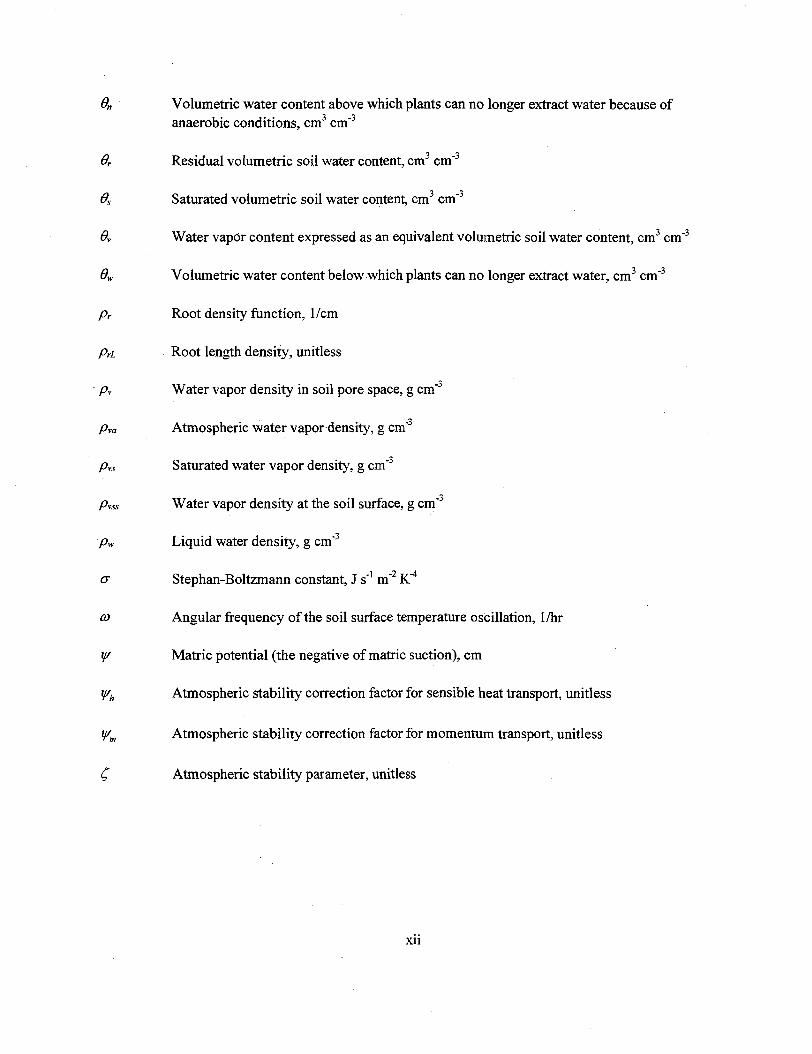
On Volumetric water content above which plants can no longer extract water because ofanaerobic conditions, cm3 cm"3

0r Residual volumetric soil water content, cm3 cm"3

0s Saturated volumetric soil water content, cm3 cm"3

By W a t e r vapor con ten t expressed as an equivalent volumetr ic soil water content , cm 3 cm"3

9V Vo lumet r i c wa t e r content be low which plants can no longer extract water , cm 3 cm"3

p r Roo t density function, I/cm

pTL Root length density, unitless

pv Water vapor density in soil pore space, g cm"3

pva Atmospheric water vapor density, g cm'3

pvs Saturated water vapor density, g cm"3

Pvss Water vapor density at the soil surface, g cm"3

pw Liquid water density, g cm"3

<y S tephan-Bol tzmann constant, J s"1 m"2 K"4

co Angular frequency of the soil surface temperature oscillation, 1/hr

y/ Matr ic potential ( the negative of matric suction), cm

y/h Atmospher ic stability correction factor for sensible heat transport, unitless

y/m Atmospher ic stability correction factor for m o m e n t u m transport, unitless

£ Atmospher ic stability parameter, unitless

XII

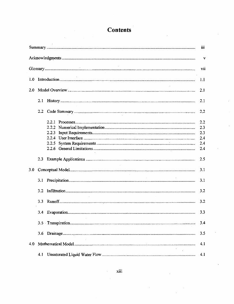
Contents

Summary iii

Acknowledgments v

Glossary vii

1.0 Introduction 1.1

2.0 Model Overview 2.1

2.1 History 2.1

2.2 Code Summary 2.2

2.2.1 Processes 2.2

2.2.2 Numerical Implementation 2.32.2.3 Input Requirements 2.32.2.4 User Interface 2.42.2.5 System Requirements 2.42.2.6 General Limitations 2.4

2.3 Example Applications 2.5

3.0 Conceptual Model 3.1

3.1 Precipitation 3.1

3.2 Infiltration 3.2

3.3 Runoff 3.2

3.4 Evaporation 3.3

3.5 Transpiration 3.4

3.6 Drainage 3.5

4.0 Mathematical Model 4.1

4.1 Unsaturated Liquid Water Flow 4.1

xin

4.2 Vapor Diffusion 4.3

4.3 Heat Flow : 4.6

4.4 Constitutive Relationships 4.7

4.4.1 Hydraulic Properties 4.7

4.4.2 Vapor Properties 4.13

4.4.3 Thermal Properties 4.13

4.5 Evaporation 4.13

4.6 Transpiration 4.15

4.7 Boundary Conditions..... 4.20

5.0 Numerical Implementation 5.1

5.1 Finite Difference Approximation of Water Flow 5.1

5.1.1 Interior Nodes 5.3

5.1.2 Surface Boundary Node 5.45.1.3 Lower Boundary Node 5.75.1.4 Mass Balance Error 5.8

5.2 Finite Difference Approximation of Heat Flow 5.8

5.2.1 Interior Nodes 5.105.2.2 Surface Boundary Node 5.115.2.3 Lower Boundary Node 5.135.2.4 Heat Balance Error 5.14

5.3 Time Steps 5.15

6.0 Code Design, Problem Formulation, and Code Operation 6.1

6.1 Code Design 6.1

6.1.1 DATAINH 6.2

6.1.2 UNSATH 6.26.1.3 DATAOUT 6.4

6.2 Problem Formulation 6.9

xiv

6.3 Code Operation : 6.12

7.0 Example Simulations 7.1

7.1 Verification of Infiltration 7.1

7.1.1 Problem Description 7.1

7.1.2 Results '. 7.2

7.2 Verification of Drainage 7.3

7.2.1 Problem Description 7.3

7.2.2 Results 7.5

7.3 Verification of Heat Flow 7.5

7.3.1 Problem Description 7.6

7.3.2 Results 7.6

7.4 Hysteresis 7.7

7.4.1 Problem Description 7.8

7.4.2 Results 7.8

7.5 Layered Soil Simulation 7.8

7.5.1 Problem Description 7.8

7.5.2 Results 7.9

7.6 Layered Soil Simulation with Heat Flow 7.10

7.6.1 Problem Description 7.10

7.6.2 Results 7.11

7.7 Transpiration Simulation 7.13

7.7.1 Problem Description 7.13

7.7.2 Results 7.13

7.8 Multiyear Simulation 7.14

7.8.1 Problem Description 7.15

7.8.2 Results 7.16

xv

8.0 References 8.1

Appendix A-UNSAT-H Version 3.0 Input Manual '. A.I

Appendix B - Input and Output Files for Example Simulations B.I

xvi

Figures

4.1 Effect of Hysteresis on Water Retention During Drying and Wetting of Silt Loam 4.10

4.2 The Ratio of Potential Transpiration to Potential Evapotranspiration as a

Function of Leaf Area Index 4.16

4.3 Relationship Between the Ratio of Transpiration to Net Radiation and Day of the Year 4.17

4.4 Root Mass at the End of the 1974 Growing Season Cheatgrass and Bluebunch

Wheatgrass Communities of the Hanford Site 4.18

4.5 The Sink Term Reduction Factor a/as a Function of Water Content 4.20

6.1 Format of the *.bin File Created by DATAINH for Input to UNSATH 6.4

6.2 Operations Flow of UNSATH 6.6

6.3 Operations Flow of DELSUB Loop in UNSATH 6.7

6.4 Format of the *.ms Output File Created by UNSATH 6.8

6.5 Example Problem Formulation: a) Site Description, b) Model Representation 6.10

6.6 Parameter Dimensions Associated with UNSAT-H Version 3.0 6.13

7.1 Infiltration Rate and Cumulative Infiltration Versus Time as Determined Using the

Philip Solution, the Numerical Code of Haverkamp et al., and UNSAT-H 7.3

7.2 Cumulative Drainage Versus Time as Determined by Kool et al. and UNSAT-H 7.5

7.3 Soil Temperature as a Function of Time (a) and Depth (b) as Determined Using an

Analytic Solution and UNSAT-H 7.77.4 Degree of Saturation Measured, Predicted by Lenhard et al., and Predicted

by UNSAT-H 7.9

7.5 Water Content Profiles Within a Layered Soil 7.10

7.6 Simulation Results for Water and Heat Flow in a Layered Soil 7.12

7.7 Soil Hydraulic Properties for the 200 Area Lysimeter 7.14xvii

7.8 Plant Parameters 7.15

7.9 Variation in Annual Deep Drainage for the Multiyear Simulation Example 7.16

Tables

4.1 Cheatgrass Root-Biomass Data, Root-Length Density, and Root Density Function 4.19

6.1 Data Flow, Program Tasks, and Subroutines 6.1

6.2 Definition of Computer Variables Used in Section 6 6.2

6.3 Subroutines in DATAINH 6.3

6.4 Subroutines in UNSATH 6.5

6.5 Subroutines in DATAOUT 6.9

6.6 Logical Unit Assignments 6.12

7.1 Parameters Used in the Infiltration Simulations 7.1

7.2 Impact of Using the Modified Picard Solution Technique 7.4

7.3 Hydraulic Property Parameters for Silt Loam Soil and Ceramic Plate 7.4

7.4 Parameters Used in the Multiyear Simulation 7.16

xvni

1.0 Introduction

The accelerating pace of development throughout the world places increasing demands on the vadosezone, which is that portion of the earth's surface that encompasses the soil and unsaturated sediments thatlie above the water table. On a site-specific basis, the vadose zone affects the movement of water,nutrients, chemicals, pathogens, and contaminants to (and sometimes from) the water table. Of specialimportance from a vadose-zone perspective are contaminants (e.g., low-level, mixed, transuranic [TRU]wastes) that have been buried in or released to the vadose zone, or the contaminants that have been or willbe disposed in special vadose zone facilities (e.g., lined landfills, vaults). In most cases, the dominantmechanism for movement is the liquid water flux, and to some extent in drier regions, the vapor flux(exceptions include nonaqueous phase liquids and gases). Thus, the successful assessment of the quantityand quality of groundwater resources depends, in part, on the ability to predict the flux of water thatmoves into and through the vadose zone. These fluxes, loosely called recharge rates, are the primarymechanism for transporting vadose zone contaminants to the groundwater. The acceptability ofcontaminants in the vadose zone is contingent on a credible demonstration that recharge rates to the watertable are less than those that would transport sufficient quantities of soluble contaminants to create anenvironmental or risk hazard.

Numerical modeling is one of the methods used to estimate the flux of water moving through thevadose zone. Field measurements of recharge rates are ideal but often expensive and of limited spatialand temporal scope. For example, the data do not exist for many of the disposal scenarios underconsideration and the data certainly do not exist for the disposal time frame of 1000 years or more. Inlieu of actual data, a recharge model can be used to assess any scenario or cover design and to makepredictions of future recharge rates given estimates of future climate and vegetation conditions.

The UNSAT-H model was developed at Pacific Northwest National Laboratory (PNNL) for assessingthe water dynamics of arid sites and, in particular, estimating recharge fluxes for scenarios pertinent towaste disposal facilities at the Hanford Site. The UNSAT-H model accomplishes this goal by simulatingsoil water infiltration, redistribution, evaporation, plant transpiration, deep drainage, and soil heat flow.

The UNSAT-H model was developed during the last several years to support the Immobilized WasteProgram (IWP) of the Hanford Site's River Protection Project. This program is designing and assessingthe performance of on-site disposal facilities to receive radioactive wastes that are currently stored insingle- and double-shell tanks at the Hanford Site (LMHC 1999). Specifically, the wastes in the tankswill be separated into high- and low-activity fractions. The high-activity fraction will be vitrified and sentto a national repository. The low-activity fraction will be vitrified, renamed immobilized low-activitywaste (ILAW), and stored in a disposal facility at Hanford. PNNL assists the IWP in performanceassessment (PA) activities associated with the ILAW disposal facility. One of the PNNL tasks is toprovide estimates of recharge rates for current conditions and long-term scenarios involving the vadosezone disposal of ILAW. Simulation modeling with UNSAT-H is one of the methods being used toprovide those estimates (e.g., Rockhold et al. 1995; Fayer et al. 1999).

1.1

This report documents XJNSAT-H Version 3.0. The report includes the bases for the conceptualmodel and its numerical implementation, benchmark test cases, example simulations involving layeredsoils and plants, and the code manual. Version 3.0 is an enhanced-capability update of UNSAT-HVersion 2.0 (Fayer and Jones 1990). New features include hysteresis, an iterative solution of head andtemperature, an energy balance check, the modified Picard solution technique, additional hydraulicfunctions, multiple year simulation capability, and general enhancements. As UNSAT-H Version 3.0 isused and evaluated, the documentation represented by this report will provide the basis for furtherevaluations and potential enhancements.

1.2

2.0 Model Overview

The two major objectives of UNSAT-H are to estimate deep drainage rates (which can then be used incontaminant transport and water resources analyses) and assist in optimizing barrier design. Toaccomplish these objectives, the model must be able to predict the near-surface water dynamics at thepertinent sites for current and postulated future climatic conditions.

2.1 History

The history of UNSAT-H begins with the UNSAT model (Gupta etal. 1978). The purpose of theUNSAT model was to predict the water dynamics of agricultural land. In 1979, the UNSAT model wasbrought to the Hanford Site and modified for waste management. The result was UNSAT-H Version 1.0,with the "H" being added to signify Hanford (Fayer et al. 1986). Although most of the mathematical andnumerical formulations of the UNSAT model that related to liquid water flow were retained in UNSAT-HVersion 1.0, the model was changed to include isothermal vapor flow, an empirical cheatgrass-transpiration algorithm, and additional hydraulic property functions.

In 1990, new capabilities were added to UNSAT-H to create Version 2.0 (Fayer and Jones 1990).These new capabilities allowed the model user to simulate soil heat flow, thermal vapor flow, and actualevaporation directly, as well as represent soil hydraulic properties with the van Genuchten water retentionfunction and the Mualem conductivity function.

Subsequent to publication of UNSAT-H Version 2.0, several revisions of the code were released toreflect error corrections and capability additions. Version 2.03, which was available for several years,was the last version to use single-precision REAL variables. Starting with Version 2.04, which was madeavailable in July 1998, double-precision REAL variables were used to achieve greater accuracy,particularly when fluxes were very low. Version 2.04 also allowed the user to modify the equation usedto partition potential evapotranspiration (PET) to reflect more accurately the transpiration rate of plantcommunities with a low leaf area index. Version 2.05 was released in April 1999 to include a couple ofminor updates and to fix a rare time-step error that led to an infinite loop. Version 2.05 represents the lastrelease prior to the release of Version 3.0.

For Version 3.0 (this report), the UNSAT-H code was modified to include hysteresis, an iterativesolution of head and temperature, an energy balance check, the modified Picard solution technique,additional hydraulic functions, multiple year simulation capability, and general enhancements. For theremainder of this report, comments concerning UNSAT-H will refer to Version 3.0, unless statedotherwise.

2.1

2.2 Code Summary

The UNSAT-H code is designed to simulate water and heat flow processes in one dimension(typically vertical). UNSAT-H can simulate the isothermal flow of liquid water and water vapor, thethermal flow of water vapor, the flow of heat, the surface energy balance, soil-water extraction by plants,and deep drainage. Information about where to find the code, updates, and lessons learned can be foundat http://hydrology.pnl.gov/.

2.2.1 Processes

Infiltration. The UNSAT-H model simulates infiltration in a two-step process. First, infiltration isset equal to the precipitation rate during each time step. Second, if the surface soil saturates, the solutionof that time step is repeated using a Dirichlet boundary condition (with the surface node saturated). Theresulting flux from the surface into the profile is the infiltration rate.

Runoff. The UNSAT-H model does not simulate runoff explicitly. Instead, it equates runoff to theprecipitation rate that is in excess of the infiltration rate. There is no provision for run-on or surfacedetention.

Soil Water and Heat Flow. The UNSAT-H model simulates liquid water flow using the Richardsequation, water vapor diffusion using Fick's law, and sensible heat flow using the Fourier equation.Convective airflow is not considered. Options for describing soil water retention include linkedpolynomials, the Haverkamp function, the Brooks and Corey function, the van Genuchten function, andseveral special functions that account for water retention of very dry soils. In addition, the van Genuchtenfunction can also be treated hysteretically. Options for describing hydraulic conductivity include linkedpolynomials, the Haverkamp model, the Mualem model, and the Burdine model.

Drainage and Lower Boundary Heat Flow. The UNSAT-H model has several options for theboundary conditions. For water flow, the user can specify Dirichlet or Neumann conditions, or a unithydraulic gradient condition. For heat flow, the user can specify Dirichlet or Neumann conditions, or atemperature gradient.

Evaporation. The UNSAT-H model simulates evaporation in two ways. In the isothermal mode,UNSAT-H uses the PET concept. The user supplies either daily values of PET or daily weather data,with which the code calculates daily PET values using the Penman equation. During each time step, thecode attempts to apply the potential evaporation rate. If the soil surface dries to or above a user-definedmatric potential limit, the time step is re-solved using a Dirichlet condition at the surface. In thissituation, the surface potential is held constant at the matric potential limit and evaporation is set equal tothe flux from below.

In the thermal mode, UNSAT-H calculates evaporation as a function of the vapor density differencebetween the soil and the reference height (the height at which air temperature and wind speed aremeasured) and the resistance to vapor transport. The resistance to vapor transport is a function of severalfactors, including air temperature, wind speed, and atmospheric stability.

2.2

Transpiration. The UNSAT-H model simulates the effects of plant transpiration using the PETconcept. There is no provision to simulate both water and heat flow in a plant canopy. Plant informationis supplied to the code to partition the PET into potential evaporation and potential transpiration. Thepotential transpiration is applied to the root zone using the root distribution to apportion it among thecomputational nodes that have roots. The withdrawal of water from a particular node is dependent on thesuction head of the node. The user provides suction head values that define how the potential transpira-tion rate applied to a particular node is reduced. Below the minimum value, sometimes known as thewilting point, transpiration is unable to remove any water. When all nodes with roots reach this level ofsuction head, transpiration is reduced to zero.

2.2.2 Numerical Implementation

The mathematical equations that describe the state and dynamics of the modeled system are written inan implicit finite-difference form. The user must specify an averaging scheme for internodal hydraulicand vapor conductivities; choices include arithmetic (and arithmetic-weighted), geometric, and harmonic.Heat internpdal conductances are calculated as arithmetic means. The resulting equations are solvedusing an iteration technique (either standard or modified Picard) with the Thomas algorithm. The solutionstrategy for each iteration is to solve the water flow equations, then solve the heat flow equations. Afterthe second and subsequent iterations, the convergence criteria are checked.

The user controls the spatial detail of the solution by specifying the node spacing in the input file.The user also controls the temporal detail by specifying the minimum and maximum time step size. Theuser can control the solution accuracy by specifying acceptance criteria for the solution to a particulartime step. The available criteria include change in water content, mass balance error, absolute change inhead, relative change in head, and heat balance error.

2.2.3 Input Requirements

The following list is a subset of the information needed to run UNSAT-H (see Appendix A for acomplete list). Not all of these inputs are needed for every simulation. Instructions for formulating aproblem to be solved and running the code are given in Section 6.0. The format for entering the data islisted in Appendix A.

Simulation Information. This information includes simulation options. Simulation options includenumber of nodes (up to 250 nodes in the compiled version), node depths and associated material types (upto 10 materials in the compiled version), boundary condition choices, output frequencies, and maximumand minimum time step size.

Constitutive Relationships. This information includes the parameters needed to describe thehydraulic, hysteretic, and thermal properties of each material, depending on the options chosen.

Initial Conditions. This information includes the initial suction head profiles and soil temperatureprofiles (if simulating heat flow).

2.3

Plant Parameters. This information includes details about the seasonal variation of leaf area indexand maximum rooting depth, root density variations with depth, and suction head limits that impact thewithdrawal efficiency of plants. UNSAT-H also has a specific function for partitioning PET intoevaporation and transpiration for Bromus tectorum (cheatgrass).

Boundary Conditions. This information includes daily PET values; daily weather conditions (e.g.,temperature, wind speed, solar radiation, precipitation); and lower boundary condition choices (e.g., waterfluxes, temperature gradient).

2.2.4 User Interface

The UNSAT-H code comprises three programs. DATAINH is used to read the text input file, processthe information, and create a binary input file. UNSATH is the main program; it reads the binary inputfile, performs the simulation, and creates a binary output file. The user runs DATAOUT to read thebinary output file. The output file contains daily (and less-than-daily if selected by the user) summariesof water content, suction head, water flow, temperature, heat flow, and plant water use as a function ofdepth. The file also contains cumulative totals of the water and heat balance components (e.g., storage,precipitation, evaporation, transpiration, drainage, net radiation, and the sensible, latent, and soil heatfluxes). The user can then view the output on screen or write the output to a text file for manipulationwith a spreadsheet or graphics program.

2.2.5 System Requirements

The UNSAT-H code is written in Compaq Visual Fortran,(a) which is based on American NationalStandard FORTRAN 77 (ANSI X3.9-1978) and FORTRAN 90 (ANSI X3.198-1992). Althoughextensions to FORTRAN 77 are available, limited use has been made of them to keep UNSAT-H close tostandard FORTRAN 77 form. The UNSAT-H code may not compile cleanly with other compilers. Theremoval of this restriction may be considered in the next revision of UNSAT-H.

The executable images for a PC require a total of 1.5 megabytes of storage. The storage required fora given output file depends on the number of nodes and length of time simulated. For the 250-nodeCLAY example in Section 7.1, the output file required 537 kilobytes of storage for the 41-day simulationusing daily output.

2.2.6 General Limitations

Features of UNSAT-H that may limit its application include one dimensionality, the use of empiricalplant transpiration algorithms, and the lack of algorithms for snowmelt, freezing soil, and the temperaturedependence of soil properties. Use of UNSAT-H is considered valid where flow is assumed to be strictlyvertical, such as in fairly level terrain or the central portion of a landfill surface cover. For steeper terrainor the edge of an elevated surface cover with sideslopes, lateral flow could be significant and thus not beamenable to analysis with a one-dimensional model. Although the one-dimensional nature of UNSAT-H

(a) Compaq Computer Corporation, P. O. Box 692000, Houston, Texas 77269-2000.

2.4

constitutes a well-defined limitation on the types of problems that can be solved, the other limitationslisted above do not. The severity of each of these limitations with respect to the intended uses of the codeis being evaluated by validation testing, which is the process by which model predictions are objectivelycompared to field or laboratory data. Testing by Fayer et al. (1992), Fayer and Gee (1997), and Khireet al. (1997) has begun to demonstrate the reliability of UNSAT-H predictions.

2.3 Example Applications

UNSAT-H can be used to solve a variety of water and heat flow problems in unsaturated soils andsediments. With proper accounting for site-specific features, recharge can be estimated as a function ofvariations in soil type or layering, plant cover and type, and climate. The applications described belowrepresent a small sample of those available. These examples are intended to give the reader a sense ofwhat has been accomplished.

The first major use of UNSAT-H was for the cover analyses used to support the Hanford DefenseWaste Environmental Impact Statement (DOE 1987). The simulations illustrated the impact of soil typeand layer thickness, the presence of plants, and weather variations on drainage through the cover. For allof these simulations, the precipitation rate was increased to twice normal (30.1 cm/yr) to evaluate whatwas then considered a worst-case situation. The results showed that coarse-textured soils such as sandswere ineffective at preventing drainage under these conditions whereas fine-textured soils were effective.The results also showed that a coarse-textured layer was needed beneath the fine-textured layer to create acapillary break. If this "break" was too deep (e.g., 3.0 m) or not present at all, the fine-textured soil couldnot prevent significant drainage from occurring.

Baca and Magnuson (1990) conducted verifications and benchmark tests of UNSAT-H. In additionto repeating the tests reported by Fayer and Jones (1990), they conducted additional tests that includedhorizontal infiltration, imposition of a constant heat flux at the surface, infiltration into a stratified vadosezone, and coupled heat and water flow in a field test plot. Baca and Magnuson judged UNSAT-H to befully operational.

Fayer and Gee (1992) used UNSAT-H to demonstrate the sensitivity of predicted drainage tohydraulic property descriptions and vapor flow. They used drainage and water content data collectedfrom a sand-filled lysimeter at the Hanford Site for comparison. They found that, of the 10 hydraulicproperty cases evaluated, 9 cases yielded drainage predictions within 10% of the measured value whenvapor flow was included. Without vapor flow, only one case yielded a drainage prediction within 10% ofmeasured value. Fayer and Gee (1992) concluded that vapor flow was a necessary process to be includedin simulations of drainage in sandy soil in semiarid climates.

Fayer et al. (1992) tested the UNSAT-H model using data from a 1.7-m deep lysimeter containing aspecific cover design. They found that the model reproduced much of the observed water balancechanges. The largest discrepancies occurred in winter (when evaporation was overpredicted) and summer(when evaporation was underpredicted). Fayer et al. (1992) demonstrated the model sensitivity to thesaturated hydraulic conductivity (K,), the pore interaction term, PET, and the presence of a snow cover(mimicked by setting PET to zero). When optimal values of these parameters were used in a single

2.5

simulation, i.e., the calibrated model, the root-mean-square error was reduced by 63% from thatdetermined with the uncalibrated model. Additional simulations were performed that indicated thathysteresis is also important to modeling of covers.

Magnuson (1993) used UNSAT-H simulations to evaluate two landfill cover designs for a disposalfacility in Idaho. He examined the sensitivity of UNSAT-H to changes in the hydraulic propertyparameters of the cover soil and the underlying gravel and cobble layers. In most cases, the changes werefactors of 0.5 and 2.0 about the base value. Drainage through this cover during the 10-year simulationswas nil, so he used the maximum predicted storage as a surrogate measure of performance, reasoning thatdrainage was most likely under those conditions when storage was at a maximum. Magnuson found thatthe hydraulic properties of the surface soil layer had the greatest impact on maximum storage. Changingthe saturated water content (#v) by 0.1 cm3/cm3 yielded a 10% change in maximum storage. Increasingthe air-entry suction head (he) of the surface soil decreased maximum storage, whereas increasing thevalue for the gravel or cobble layers increased maximum storage slightly. Changing the Ks value of thesurface soil decreased maximum storage. Apparently, precipitation could infiltrate the soil more deeply,but it was easier for evaporation to extract that water later. Changes to the Ks of the gravel and cobblelayers had no discernible effect on maximum storage.

Magnuson (1993) also evaluated the sensitivity to the same parameters for the case where the coverwas a single soil material with no layering. For these simulations, drainage was detectable so it was usedas the performance measure. Magnuson found that drainage changed inversely with changes in 0,. Forexample, as 0S was changed from 0.5 to 0.4, drainage increased by 89% (from 1.36 to 2.58 cm/yr).Changing the residual water content (0r) from 0.007 to 0.056 increased drainage by 36%. Increasing he

from 21 to 60 cm reduced drainage by 91%. Magnuson looked at a second soil type and found that themodel responses to the changes were sometimes different. For example, increasing the Ks of the secondsoil type increased drainage, in contrast to the first soil type in which drainage decreased with increasingKx. The importance of this result is that parameter sensitivities can be dependent on the conceptual modeland so should be determined on a case-by-case basis.

Fayer and Gee (1997) used a 6-year record of water storage, suction, and drainage data to testUNSAT-H. This comparison was an extension of the work by Fayer et al. (1992). The data werecollected from a non-vegetated weighing lysimeter containing 1.5 m of silt loam over sand and gravel.This capillary-break layering configuration was designed to promote water storage in the upper layer foreasier removal by evapotranspiration. Four simulations were conducted: 1) standard parameters,2) calibrated parameters, 3) heat flow, and 4) hysteresis. The water storage results showed littledifference among the four simulations; the root mean square (RMS) errors were all between 23.4 and23.7 mm. Fayer et al. (1992) reported an RMS error of 8.1 mm for the calibrated simulation during thefirst 1.5 years. Beyond the calibration period, however, the calibrated model was not much moresuccessful than the other models in predicting total water storage.

The standard parameters, heat flow, and hysteresis simulations had the largest maximum storagedifference (75 to 80 mm); the calibrated simulation had the smallest (59.3 mm). This result may be onebenefit of the calibration, the goal of which was to match the peak water storage in winter. In contrast,

2.6

the calibrated simulation had the largest mean and median differences (19.6 and 16.4 mm, respectively).The other simulations had values between -6.0 and 3.0 mm.

All of the simulations almost always overpredicted suction heads, more so in the summer than thewinter. The hysteresis simulation gave the best qualitative match of suction heads throughout the 6-yearperiod. At times, the predictions coincided with the measurements, most importantly during the one andonly drainage event observed in 6 years. The other three simulations predicted suction heads that weregenerally at least a factor of 3 greater than the measured values.

The hysteresis simulation was the only one to predict drainage. The predicted cumulative drainagewas within 52% of the measured amount and the timing matched the observations. Fayer and Gee (1997)attributed the success of the drainage prediction to the ability to simulate suction heads at the interface.They suggested that suction head is better than water storage as an indicator of conditions at the silt loam-sand interface that control drainage.

Based on the comparisons, Fayer and Gee (1997) reached several conclusions. First, UNSAT-H canreasonably predict the water balance components of a capillary-break type cover. The predictionsimprove if the hysteresis phenomenon is included. Second, the inclusion of heat flow has only a minoreffect on surface evaporation and vapor flow within the soil. The impacts of heat flow on snowaccumulation and melt and on soil freezing were not evaluated, but Fayer and Gee (1992) speculated thatthese impacts could be important. Finally, a calibrated model will not necessarily apply well outside ofthe calibration period. Fayer and Gee (1997) offered suggestions for improving the calibration process:1) include a more complete conceptual model (e.g., including hysteresis), 2) use multiple performancemeasures, and 3) calibrate with a period of time sufficiently long to encompass the range of conditionsenvisioned for the design life of the cover.

Khire et al. (1997) applied the UNSAT-H and HELP models to resistive barrier test cells at theGreater Wenatchee Regional Landfill in Washington and the Live Oak Landfill in Georgia. TheWenatchee landfill is in a semiarid climate; the Live Oak landfill is in a humid climate. The authorstested the models using a 3-year record of dataihat included overland flow, soil water storage,evapotranspiration, and percolation. The results, in the form of time series plots, showed that the modelsgenerally mimicked the seasonal trends. The authors stated that the UNSAT-H predictions tended to bemore accurate that those using HELP. With respect to UNSAT-H, the authors noted several conceptualfeatures that were important to the Wenatchee site but were not included in the model: snow cover, snowmelt, and freezing soil. Based on their experience with simulating these two landfills, Khire et al. (1997)suggested that practitioners use a simpler model (e.g., HELP) during the iterative design phase and a morecomplex model (e.g., UNSAT-H) for final checks.

Fayer et al. (1999) conducted a set of simulations to estimate recharge rates for scenarios pertinent tothe 2001 ILAW PA. The scenarios included the surface cover (1 m of silt loam over sand and gravel) andtwo surrounding soil types, as well as two types of surface cover degradation. The simulations wereconducted using a 41-year sequence of weather collected at the Hanford Site from 1957 to 1997. Thesimulation results indicated that the surface cover would limit drainage to < 0.1 mm/yr, which is lowerthan the cover design goal of 0.5 mm/yr. The cover maintained this performance level for almost all

2.7

scenarios evaluated, including plant removal, wetter and cooler climate, and erosion of 20 cm of the siltloam layer. The cover also maintained this performance when 20 cm of windblown sand was depositedon the cover under current climate conditions. Under 7 of the 8 future climate scenarios, the predicteddrainage rates continued to be < 0.1 mm/yr. Only under the future climate scenario of wetter and coolerweather was significant drainage (16.9 mm/yr) simulated, even though shrub-steppe vegetation waspresent. This simulation was intended to stress the system. While the record indicates periods of coolerweather and periods of wetter weather, the record does not indicate their concurrent occurrence. Instead,cooler weather appears to result in drier conditions. Additional simulations highlighted modelsensitivities to further variations in climate, soil hydraulic properties, plant parameters, and irrigation.

2.8

3.0 Conceptual Model

A conceptual model of the near-surface water dynamics of a site identifies the features and processesthat are thought to significantly influence the flow of water in soil. The development of a site-specificconceptual model for water flow in unsaturated soil begins by formulating a site-specific water balanceequation to partition the water at a site into three categories: input, output, and storage. On the soilsurface, precipitation (P) represents the input and infiltration (I) and runoff (Rotf, the amount that runs offthe surface) represent the outputs. Overland flow that runs onto a site (i.e., run-on) would be an input tothe system, but this process is not included in the UNSAT-H conceptual model. Precipitation couldcollect in depressions on the soil surface or on the surfaces in the plant canopy, but these water storagemechanisms are not included in the UNSAT-H conceptual model. With no water storage allowed, theequation for the water balance above the soil surface becomes

0 = P-I-Roff (3.1)

Once water has infiltrated the soil, the soil water balance equation that forms the basis of theUNSAT-H conceptual model is

ASW=I-E-T-D (3.2)

where ASW is the change in soil water storage during an interval of time. Water storage is the averagevolumetric water content of the soil multiplied by the depth of soil. The water balance equation simplystates that the change in the amount of water stored in the soil profile is equal to the total infiltrationminus the amount of water that is lost to evaporation, E; transpiration, T; and drainage, D.

The second step in developing the conceptual model is to identify the environmental processes andphysical principles controlling each term in Equation (3.2). For example, the flow of heat to the soilsurface affects the rate of evaporation. Based on the interrelationships among terms in Equation (3.2),any attempt to solve for the value of one term will be limited by the accuracy of the other terms.

3.1 Precipitation

Annual precipitation at the Hanford Site has averaged about 17.3 cm since 1946, ranging from lessthan 7.6 cm to 31.3 cm (Hoitink et al. 1999). In addition to low annual rates, precipitation at the HanfordSite is highly seasonal, with an average of 60% of the annual total coming between October and February.During these months, a significant percentage of precipitation may occur as snow. In fact, snow typicallyaccounts for 22% of the annual precipitation and 37% of the winter total.

The seasonal character of precipitation and the significant proportion as snow raise two issues thatmust be addressed by the conceptual model. The first issue is whether to explicitly account for snowfalland snowmelt, or to treat snow as an equivalent amount of rain. Snow covers the ground at the HanfordSite an average of 22 days per year, but may range from 0 to 60 days. The presence of a snow cover may

3.1

both delay the entry of water into the soil and affect evaporation rates. The present conceptual modelincorporated into UNSAT-H, however, views snow as an equivalent amount of rain. The UNSAT-Hmodel does not attempt to simulate snowmelt or the effects of snow cover on evaporation, nor does itaccount for sublimation.

The second issue related to winter precipitation is how frozen soil affects infiltration, redistribution,evaporation, and runoff. If the climate at the Hanford Site were such that precipitation were negligibleduring winter months,' then the effects of soil freezing would likely be small. However, the presence ofsignificant precipitation during winter months means that frozen soil may need to be considered. Themonthly weather records for the Hanford Site indicate that average temperatures at the 38-cm depth havebeen as low as -3.6°C. The need for future modifications of UNSAT-H (e.g., to simulate snowmelt andfrozen soil) is being investigated.

3.2 Infiltration

Infiltration is the process of water entry into soil. The instantaneous infiltration rate, called the soilinfiltrability, is a function of several factors, including the time from the onset of precipitation (or irriga-tion), the initial water content, the hydraulic properties of the surface soil, and the hydraulic properties oflayers deeper within the profile (Hillel 1980). At the start of an infiltration event, the instantaneousinfiltration rate is maximal. In time, the rate decreases asymptotically to a value approaching thesaturated conductivity of the surface soil. As the wetted depth of soil increases, the infiltration ratedecreases asymptotically and approaches the saturated conductivity of the most impeding layer within thewetted portion of the profile. The process can be viewed in two stages. In the first stage, infiltration iscontrolled by the supply of water (i.e., supply-controlled or flux-controlled). This situation is typical ofnearly all precipitation events at the Hanford Site. In the second stage, infiltration is controlled by the soilprofile conditions. Many algebraic equations have been developed to estimate infiltration rates duringthis second stage. However, the UNSAT-H conceptual model does not use an infiltration equation.Instead, infiltration is determined directly by calculating the ability of the soil profile to transmit waterdownward. Section 3.6 describes the conceptual model for soil water redistribution within the profile.

3.3 Runoff

When the precipitation rate exceeds the infiltration rate, water begins to accumulate on the soilsurface. Overland flow occurs when the soil's water-detention capacity is exceeded and the surface isslightly sloped. Overland flow is unlikely to occur during rainfall at the Hanford Site because theinfiltration capacities of most of the soils exceed several centimeters per hour, in contrast to the 1000-yearstorm intensity of less than 3 cm/hr for 1 hr (Hoitink et al. 1999). Higher storm intensities are probable,but for shorter periods of time. Regardless of precipitation intensity, overland flow may occur when asnow cover melts quickly and the soil beneath is frozen (such that the soil's infiltrability is severelyrestricted). Localized overland flow has been observed at the Hanford Site under such conditions.

Overland flow is not addressed by the UNSAT-H conceptual model, partly because the processoccurs so rarely, but mostly because UNSAT-H is a one-dimensional model. When overland flow does

3.2

occur, it is caused, in part, by variable surface topography. Overland flow is a multidimensional processthat a one-dimensional model cannot describe. For a one-dimensional model to be applicable, theproblem must be formulated such that water is applied uniformly over the surface. Therefore, UNSAT-Hcan be applied only to areas for which local run-on/runoff processes can be represented by a uniformprecipitation rate over the entire area of interest, or to areas in which overland flow is prevented, such asin lysimeters.

3.4 Evaporation

Evaporation is the process of water loss from soil and/or plant surfaces to the atmosphere.Evaporation of water from the soil surface is controlled by the flow of heat to and from the soil surface,the flow of water to the soil surface from below, and the transfer of water vapor from the soil surface tothe atmosphere (Hillel 1980). If any of these processes is altered, evaporation will change accordingly.

An integrated form of Fick's law of diffusion (the equation used to model vapor flow within the soilprofile) addresses the interrelationships of these three processes and, therefore, has the structure necessaryto predict evaporation. This form of Fick's law simply states that the evaporation rate is equal to thedeficit in vapor density between the soil surface and the atmosphere divided by the atmosphericboundary-layer resistance. The atmospheric boundary layer is defined as the region of the atmospherethat is directly affected by the shearing forces originating at the surface. Rosenberg et al. (1983) refer tothis layer as the turbulent surface layer. Air temperature, vapor density, and wind speed are measuredwithin the atmospheric boundary layer.

The integrated form of Fick's law accounts for the potential effects that each of the three processesidentified above may have on evaporation. For the first process, heat flow, a rising soil-surfacetemperature causes the vapor density at the soil surface to increase. This increased vapor density, in turn,increases the vapor density deficit between the soil surface and the atmosphere, and a higher evaporationrate thus ensues. Falling surface temperature has the opposite effect of reducing the deficit, thus loweringthe evaporation rate.

In the second process, water flow, a decrease in the supply of water to the surface leads to surfacedrying. A drier surface has a lower vapor density; hence, the vapor density deficit is smaller andevaporation is reduced. An increased supply of water to the soil surface would have the opposite effect.

The third process, transporting water vapor from the soil surface to the atmosphere, is controlled byboth the atmospheric vapor density and the atmospheric boundary-layer resistance. Generally, the soilsurface is wetter (higher vapor density) than the air. If the atmosphere is moist, however, such as duringthe early morning when temperatures approach the dew point or following precipitation, the increasedatmospheric vapor density decreases the surface-air vapor deficit and, therefore, decreases evaporation.Another way that the transfer of water vapor from the soil surface to the atmosphere can be reduced is bydecreased wind speed or reduced eddy diffusion caused by high atmospheric stability.

UNSAT-H has an alternate conceptual model for evaporation in which the soil is isothermal. For thisconceptual model, the diffusion equation for evaporation can be shown to be equivalent to Penman-type

3.3

equations. The Penman equation and its derivatives (Monteith 1980) are attempts to rewrite the diffusionequation to exclude the explicit dependence of the rate of diffusion on soil-surface temperature. Penman-type equations attempt to replace the need for data on soil surface temperature with information on netradiation and soil heat flux.

When the soil surface is very wet, as immediately after a heavy rainfall, the evaporation rate will be ata maximum. This maximum rate, termed potential evaporation (Ep), is determined largely by atmosphericparameters that control the supply of energy to and from the surface and the transport of water vaporaway from the surface. The isothermal conceptual model in UNSAT-H assumes that Ep can be calculatedsolely based on atmospheric parameters, thus ignoring the effects of soil surface temperature and watercontent on the evaporation rate.

Given this conceptual model, the actual evaporation rate from a soil surface is equal to Ep for only thefew hours immediately following rainfall. More often, the evaporation rate is much lower than Ep

because, as water evaporates from the soil, the soil profile begins to dry, particularly near the surface.Dry soil is a poor conductor of water and cannot readily transmit water from the moist, deeper layers tothe evaporating surface at a rate sufficient to maintain the Ep rate. Thus, drying of the soil limits actualevaporation to a rate that is generally a small fraction of Ep. Because of the dryness of Hanford Site soils,an important concept in this evaporation model is that the evaporation rate is limited primarily by soilconditions, rather than atmospheric conditions.

At times, usually nighttime, the atmospheric vapor density can exceed the soil surface vapor densityand result in the formation of dew. This form of water addition to the soil is not part of the currentUNSAT-H conceptual model.

3.5 Transpiration

Transpiration is the evaporation of water from plants. When the soil surface is well vegetated withactive plants, transpiration is usually the dominant mode of water loss from the soil profile. Even whenthe surface is only sparsely vegetated, transpiration can rival evaporation as the primary source of waterloss from the soil. Exceptions to the above may occur during certain times of the year when plants aredormant or reacting to extreme water stress.

In their Hanford Site characterization report to satisfy the requirements of the National EnvironmentalPolicy Act, Neitzel et al. (1999) identified shrublands as the areally predominant vegetation community atthe Hanford Site. This community, commonly called shrub-steppe, includes big sagebrush, three-tipsagebrush, bitterbrush, gray rabbitbrush, and spiny hopsage. Grasses and forbs typically make up theunderstory in these communities. Grasslands are another areally extensive community. Bluebunchwheatgrass dominates at the upper elevations and shares space with Sandberg's bluegrass and cheatgrass(an alien species) at the lower elevations. At many locations, particularly those that have been disturbed,cheatgrass has become the dominant species. This change is important because cheatgrass, which hasshallow roots, tends to crowd out the native species, some of which can have deep roots. Gee and Heller(1985) reported that rooting depths range from less than 100 cm for cheatgrass to 200 cm for sagebrush,

3.4

220 cm for rabbitbrush, and 300 cm for bitterbrush. Gee (1987) reported that this rooting-depthdifference can lead to increased recharge under cheatgrass communities.

Annual water loss by transpiration at the Hanford Site is less than potential transpiration (Tp), just asannual evaporation is less than Ep. The reduction of transpiration below the potential rate is causedprimarily by two mechanisms. The first mechanism involves a decrease in plant biomass, primarily leafarea; the second mechanism involves stomatal closure.

When plants are stressed by lack of water, they may lose leaves, shoots, and roots. This reduction inplant tissue means that less water is necessary to maintain the remaining biomass. Reduction of plantbiomass is a relatively slow mechanism that responds to climatic conditions averaged over weeks ormonths. On a short-term (e.g., hourly) basis, water loss can be reduced by stomatal closure. Closing ofstomata (small openings in the leaves) drastically reduces plant water loss. In addition, closure of thestomata reduces carbon dioxide uptake, which limits photosynthesis and reduces overall plantmetabolism.

The UNSAT-H conceptual model of transpiration relies on estimates of a potential evapotranspirationrate (PET) that is calculated from climate data. That potential rate is then modified by a "crop" coeffi-cient that is a function of either leaf area or time of year. The resulting Tp is applied to specific depthswithin the soil profile in proportion to the fraction of roots at these respective depths.

UNSAT-H currently allows for a fixed distribution of roots in the profile throughout the year and avariable maximum depth of root penetration. This conceptual model of transpiration offers someflexibility to vary transpiration during the simulation, but only in a predetermined way, and never solelyin response to the conditions of the specific simulation. Some of the plant communities at the HanfordSite are mixed. That is, they include perennial as well as annual species, each with its own life cycle androoting characteristics that influence the composite annual transpiration distribution. Caution should beexercised when the UNSAT-H model is applied to such plant communities until more information isavailable on the behavior of mixed plant communities.

3.6 Drainage

The final term of Equation (3.2) is drainage, which is the movement of water downward through thebottom of the zone being simulated. Of particular interest is the drainage water that reaches the watertable. This specific type of drainage is known as groundwater recharge. As a practical matter, once waterdrains below the root zone, there is little chance of it being drawn upward again. Therefore, recharge isoften defined as drainage below the root zone. Recharge is perhaps the water balance term of mostinterest for waste management because of its potential to move contaminants out of waste-disposal sites.A primary objective of any waste-disposal facility is to reduce recharge, and thus reduce the potential fordrainage of water through the waste material.

Drainage results from the redistribution of water through a soil system in response to gradients in theenergy state of the water. Other mechanisms that might induce water redistribution, such as geothermalgradients and barometric pressure fluctuations, have been shown to be minor contributors to water flow in

3.5

soils at the Hanford Site (Reisenauer et al. 1975; Jones 1978; Gee and Simmons 1979). The energy stateof water is expressed as a potential energy, commonly assumed to consist of a gravitational potential,pressure or matric potential, and solute potential. All of these potentials are expressed relative to theenergy state of pure water at atmospheric pressure and a reference elevation.

Pressure or matric potential describes the water pressure difference from atmospheric pressure. Whenthe water pressure is greater than the atmospheric pressure, the soil is saturated and the term pressurepotential is used. When the water pressure is less than the atmospheric pressure, the soil is unsaturatedand the term matric potential is used. Nearly all applications of UNSAT-H will be for unsaturatedproblems; consequently, the convention is to use matric potential.

The solute potential, which is the drop in potential energy caused by the presence of solutes, iseffective in contributing to water flow only when there is a differential restriction of solute movementrelative to water. In the absence of a semipermeable membrane, the solute potential is commonlyneglected. In the conceptual model, therefore, the energy state of water is described by the sum of thegravitational and matric potentials; the sum is usually called the hydraulic potential. Water continuallyredistributes from areas of high hydraulic potential to areas of low hydraulic potential, regardless ofdirection.

A question that must be addressed by the conceptual model is whether to include the flow of watervapor in the redistribution and drainage calculations. The above discussion of water redistribution inresponse to potential gradients applies mainly to water in the liquid phase. In unsaturated soils, water isalso present in the vapor phase. Water vapor moves and redistributes within the soil in response to vaporpressure gradients. These vapor pressure gradients can arise from matric and osmotic potential gradientsin the liquid phase and from temperature gradients within the soil. In the absence of a semipermeablemembrane that could produce osmotic potential gradients, osmotic potential is not part of the UNSAT-Hconceptual model. Water vapor flow induced by matric potential gradients is known as isothermal vaporflow. Vapor flow induced by thermal gradients is known as thermal flow.

Analyses like that of Campbell (1985) imply that isothermal vapor flow can affect the near-surface(top 10 cm) water-content profile, although it is unclear how this would affect long-term simulations ofthe water balance. Thermal vapor flow affects evaporation when the surface soil is dry and steep thermalgradients are present, a condition that occurs frequently at the semiarid Hanford Site. Hammel et al.(1981) reported that exclusion of thermal vapor flow resulted in a higher predicted evaporative loss andpoorer agreement between measured and predicted moisture profiles in a seed zone. Therefore,UNSAT-H can recognize that vapor flow has a thermal component.

Water redistribution (and thus drainage) is dependent on the soil hydraulic properties, which aredescribed using mathematical functions. In some cases, a property is significantly affected by its priorvalues in addition to the current state of the system. This non-uniqueness of a property is calledhysteresis. Soil hydraulic properties that are hysteretic have been shown to affect soil water flow in somesituations (Gillham et al. 1979; Kool and Parker 1987; Lenhard et al. 1991). One of the available

3.6

hydraulic functions (the van Genuchten function) is implemented in a hysteresis model within UNSAT-H.The remaining soil hydraulic property functions in the UNSAT-H conceptual model are unique (i.e., theyexhibit no hysteresis).

Soil hydraulic properties and the diffusion coefficient of water vapor through air are somewhatdependent on temperature. Nimmo and Miller (1986) determined that the temperature dependence ofwater potential is much greater than that which would result from just the dependence of surface tensionon temperature. Currently, however, the soil properties of the UNSAT-H conceptual model are assumedto be independent of temperature.

Deep below the soil surface, temperature gradients are assumed to have a negligible effect onredistribution of water. Near the soil surface, however, steep temperature gradients can exist and be thedominant cause of water vapor diffusion. Heat flow near the surface also plays a major role in deter-mining the evaporation rate. Heat may be transferred within the soil by different mechanisms. Heattransported by conduction or by convection within moving liquid, vapor, or air is known as sensible heat.Heat associated with a phase change is known as latent heat. The latent heat associated with the phasechange between liquid and vapor may be transported convectively or diffusively by water vapor. Thelatent heat associated with melting ice can be transported convectively by moving liquid water. Heat canalso be transmitted through radiative transfer. All materials at a temperature above absolute zero radiateenergy in the form of heat.

The current conceptual model of heat flow within the soil includes the conduction and convection ofsensible heat and the diffusive transport of latent heat of vaporization. The UNSAT-H conceptual modeldoes not address the convective transport of latent heat associated with soil freezing or thawing, radiativeheat transfer within the soil profile, or ice formation. The contribution from these processes to the soilenergy balance is assumed to be small. At the soil surface, convective and radiative heat flow processesbetween the soil and atmosphere are considered in the conceptual model.

3.7

4.0 Mathematical Model

The mathematical model consists of a set of differential equations and boundary conditions thatquantify the conceptual model by describing the processes depicted in Equation (3.2). In this section, themathematical models for unsaturated liquid water flow, vapor flow, heat flow, evaporation, andtranspiration are presented.

In discussions of soil water flow for unsaturated conditions, hydraulic potential is calculated as thesum of the gravitational and matric potentials. The fundamental expression of potential is in terms ofenergy per unit mass. It is much more convenient and common, however, to replace the term potentialwith head, which is energy per unit weight and has units of centimeters. Therefore, the total potential isgiven as the hydraulic head, H; the gravitational potential as the gravitational head, Z; and the matricpotential as the matric head, ij/.

4.1 Unsaturated Liquid Water Flow

The differential equation for liquid water flow is a modified form of Richards' equation (Richards1931). This equation describes the change in water storage, redistribution, and plant water uptake atevery point within the soil profile. The flow of water across either boundary of the profile is representedby specifying a flux (e.g., precipitation, evaporation, or drainage) or by calculating a flux either directly(e.g., evaporation as a diffusive flux) or indirectly (e.g., holding the value of the boundary-node headconstant for such boundary conditions as a ponded surface, evaporation, or a water table).

The development of the modified Richards' equation begins with Darcy's law. In its original form,Darcy's law represented an empirical relationship between the rate of flow in saturated sand and thehydraulic head gradient. The one-dimensional differential form of Darcy's law (Hillel 1980) is

T. oH ,, , ,K C41)

where qL is flux density of water, cm hr"1; Ks is saturated hydraulic conductivity, cm hr"1; and z is depthbelow the soil surface, cm. Darcy's law can be extended to unsaturated flow by replacing the saturatedconductivity term with liquid conductivity, KL, as a function of matric head, yielding

qL=-KL{yf)~ (4.2)dz

Equation (4.2) must be combined with the continuity equation to describe transient flow. The continuityequation states that the change in water content of a volume of soil must equal the difference between fluxinto and out of the soil volume. For one-dimensional flow, the continuity equation is

4.1

dt dz( 4 .3 )

where 0is the volumetric water content, cm3 cm"3; and / is time, hr. Combining Equations (4.2) and (4.3)yields

de a [ F , m\-z- = T \KL(V)—\ (4-4)dt dz L d J

UNSAT-H has two sign conventions that relate to heads. The first convention concerns gravitationalhead. With the soil surface as the reference elevation, the gravitational head at a point in the soil is theelevation of the point with respect to the soil surface and thus is negative. Because depth measured fromthe surface is positive, the gravitational head equals the negative of soil depth. Therefore, in UNSAT-H, zis replaced with -z. The second convention concerns matric head, which is a negative number forunsaturated soil conditions. In UNSAT-H, matric head is replaced with suction head, h, which is thenegative of matric head. Thus, a positive suction head represents a matric head, and a negative suctionhead represents a pressure head. The calculation of hydraulic head then changes from H= y/ + Z to theUNSAT-H form

H = -(h + z) • (4.5)

Using the chain rule of differentiation, dd/dt in Equation (4.4) can be replaced by C(h) (dh/dt), where C(h)represents dO/dh (i.e., the negative of the specific moisture capacity). With this manipulation and theincorporation of the identity h = -y/, Equation (4.4) becomes

Combining Equations (4.5) and (4.6) and adding a sink term, S, for water uptake by plants gives

C(A)—= - — KL(h{— + l\ -S(z,t) (4.7)dt dz\_ \dz J

where S(z,t) indicates that the sink term is a function of depth and time. With slight rearrangement,Equation (4.7) is the same as that in Gupta et al. (1978), Gee and Simmons (1979), and Simmons and Gee(1981).

The assumptions that led to Equation (4.7) are

• fluid is incompressible

• air phase is continuous

4.2

• air phase is at constant pressure

• flow is one-dimensional

• liquid water flow is isothermal

• vapor flow is negligible.

The first three assumptions are routinely made for modeling of soil water under unsaturatedconditions and are considered valid for the Hanford Site. The fourth assumption, one-dimensional flow,is considered valid for most near-surface modeling efforts, provided the surface is uniform and nearlylevel, no overland flow exists, and soil properties are homogeneous and isotropic within each defined soillayer. The fifth assumption, isothermal liquid flow, is considered valid for the Hanford Site. The finalassumption, that vapor flow in negligible, is not considered valid. Soils at the Hanford Site dry outsignificantly during the summer and liquid-water conductivities decrease dramatically, to a point at whichdiffusion of water vapor from the soil to the atmosphere can be the dominant mode of water loss. Vaporflow is considered in the next section.

4.2 Vapor Diffusion

The fundamental equation used to calculate the diffusion of water vapor in soils is Fick's law ofdiffusion, which can be written as

* f <>Pw dz

where qv = flux density of water vapor, cm hr"!

pw = density of liquid water, g cm"3

D = vapor diffusivity in soil, cm2 hr"1

pv = vapor density, g cm"3.

When applying Fick's law to soils, adjustments must be made to account for the tortuous diffusionpath and the reduced cross-sectional area available for flow. The need for both adjustments arises fromthe three-phase nature of soils. The usual way these adjustments are included in Equation (4.8) is to writethe diffusivity term as

D = a{6s-e)Da (4.9)

where a is the tortuosity factor; Da is the diffusivity of water vapor in air, cm2 s"1; and the quantity (9s-6)represents the air-filled porosity. Many variations of Equation (4.9) exist (Marshall 1959; Currie 1965;Troeh et al. 1982); however, they generally treat or as a constant or as a function of air-filled porosity.The most common formulation is to set a equal to 0.66 (Penman 1940; van Bavel 1952).

4.3

Fick's law can be written to explicitly include gradients for suction head and temperature by using thechain rule of differentiation to rewrite the vapor density gradient. Equation (4.8) becomes

Dd£d±Ddp&L ( 4 1 Q )

pw dh dz pw dT dz

where T is the temperature, K.

The vapor density at a specific point in the soil can be related to the saturated vapor density, pvs, andrelative humidity, HR, by

PV=PVSHR (4-11)

Because water vapor density is a function of relative humidity and temperature, Equation (4.10) can berewritten. Combining Equations (4.10) and (4.11), using the product rule for differentiation and assuming8HR/dT = 0 (Philip and deVries 1957), Fick's law can be written as

f.f (4.12)dT dpw dz pw

Equation (4.12) explicitly includes the effect of soil temperature on vapor diffusion. The first termrepresents isothermal vapor diffusion. The second term represents thermal vapor diffusion. From the soilsuction head, the relative humidity can be determined using (Campbell 1985)

HR = exp| -hMg

RT(4.13)

where Mis the molecular weight of water, g mole'1; g is the gravitational constant, cm s"2; and R is the gasconstant, erg mole'1 K"1.

Much work has been published that evaluates the validity of Eiquation (4.12), particularly the thermalvapor diffusion term. Experimental measurements show that Equation (4.12) underpredicts water vaporflow. This deficiency is particularly apparent when temperature gradients are present (Gurr et al. 1952;Taylor and Cavazza 1954; Philip and de Vries 1957; Cassel et al. 1969; Cass et al. 1984). Mostresearchers have assumed that the problem is with the thermal vapor diffusion term of Equation (4.12);however, Scotter (1976) presents evidence that the isothermal term is also incomplete.

The most widely accepted explanation of why Equation (4.12) fails was proposed by Philip and deVries (1957). They suggest two features that could be responsible for vapor diffusion greater than thatpredicted by Fick's law. The first is that the measured temperature gradient in a soil underestimates thetemperature gradient within the air phase of the soil pores, and this "microscopic" temperature gradient isthe more appropriate value to use in Fick's law. Second, Philip and de Vries (1957) propose that vapor iseffectively transported through the liquid phase by condensation and evaporation processes operating

4.4

within individual pores. These processes would have the effect of increasing the cross-sectional areaavailable for vapor diffusion to a value larger than that for air-filled porosity and of decreasing thetortuosity or path length for diffusion. Philip and deVries (1957) proposed adding an enhancement factor,rj, to the thermal vapor diffusion term in Equation (4.12) to account for these two processes.

Substituting the enhancement factor into Equation (4.12) and expressing the HR gradient in terms ofthe gradient in h gives the following formulation of Fick's law:

.....(4.14)

This law explicitly accounts for the effect of temperature gradients and enhanced vapor diffusion in soil.

The first term on the right-hand side of Equation (4.14) is referred to as the isothermal vapor fluxdensity, qv/,- Although considered the isothermal flux, it does allow for the saturated vapor densitythroughout the soil to vary according to the simulated soil temperature, rather than being a constant basedon a fixed value of soil temperature. The second term on the right-hand side of Equation (4.14) isreferred to as the thermal vapor flux density, qvr.

The qVh and qrj terms in Equation (4.14) are similar to the flux equation for liquid flow. As such,most of the parameters can be combined to yield vapor conductivity terms. The isothermal vaporconductivity term, Kvh, is

_Kvh= PwK1

The thermal vapor conductivity term, KrT, is

Equation (4.7) can now be rewritten to include the contribution of vapor flow

C(h)^ = -piKT(h)^ + KL(h) + qvT}-S(z,t) (4.17)at az\_ oz J

where Kj is Ki + KVf,. Equation (4.17) is the modified Richards' equation that serves as the primarydifferential equation solved by UNSAT-H; it describes changes in water storage, isothermal redistributionof liquid water, nonisothermal redistribution of water vapor, and water uptake by plants. This equation isapplied at every point in the interior of the soil profile.

4.5

4.3 Heat Flow

Calculation of soil temperature requires solving the energy balance equations in much the samemanner that the soil water-balance equations are solved to obtain soil water potential. The constitutiveequation describing the conduction of sensible heat is Fourier's law of heat conduction

where qh is the heat flux density, J cm"2 hr"1; and kh is the thermal conductivity of soil, J cm"1 hr"1 K'1.

The latent heat transported by vapor flow is equal to the product of the latent heat of vaporization andthe flux density of water vapor, which is calculated using Equation (4.14). The heat convected by waterflow is equal to the product of the heat capacity of water, the flux density of water, and the soiltemperature. Adding latent and convective heat transport to Equation (4.18) gives the steady-state heatflux density (Jury 1973):

qh=-kh— + Loqv+Chv{T-To)qv+Chw{T-To)qL (4.19)

where Lo is the volumetric latent heat of vaporization of water, J cm"3, at the reference temperature T,» andChv and Chw are the volumetric heat capacities of water vapor and liquid, J cm"3 K"1.

Relative to the reference temperature, the storage of heat (Sh) in the soil is

Sh =Chs{T-To) + Lo0v+Chv{T-To)0v+Chw(T-To)e (4.20)

where Chs is the volumetric heat capacity of dry soil particles, J cm"3 K"1, and 6V is the volumetric vaporcontent expressed as an equivalent water content. The continuity equation for the conservation of energyin one dimension is (Jury 1973)

(4.21)dt dz

Combining the continuity equation with Equation (4.19) gives the soil temperature equation to be solvedbyUNSAT-H:

Ch-Z7 + Lo - r ~ + chv\T - TO)-T- + chw\T - ro,J-r- =dt dt dt dt

(4.22)

4.6

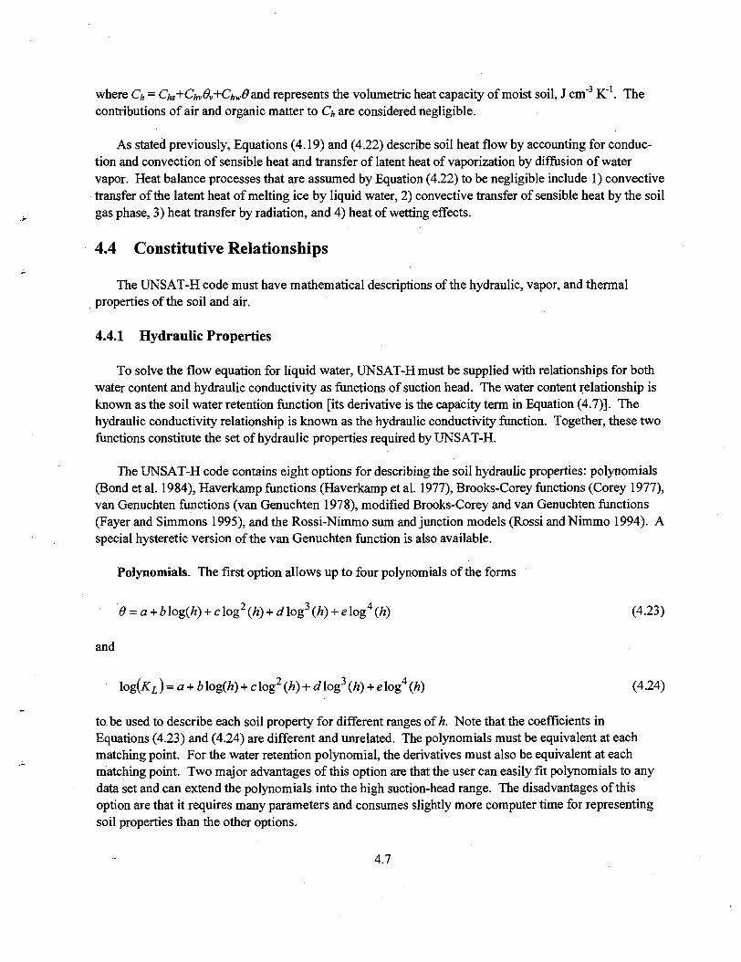
where Cy, = Chs+CfoOv+Chwd and represents the volumetric heat capacity of moist soil, J cm'3 K"1. Thecontributions of air and organic matter to C/, are considered negligible.

As stated previously, Equations (4.19) and (4.22) describe soil heat flow by accounting for conduc-tion and convection of sensible heat and transfer of latent heat of vaporization by diffusion of watervapor. Heat balance processes that are assumed by Equation (4.22) to be negligible include 1) convectivetransfer of the latent heat of melting ice by liquid water, 2) convective transfer of sensible heat by the soilgas phase, 3) heat transfer by radiation, and 4) heat of wetting effects.

4.4 Constitutive Relationships

The UNSAT-H code must have mathematical descriptions of the hydraulic, vapor, and thermalproperties of the soil and air.

4.4.1 Hydraulic Properties

To solve the flow equation for liquid water, UNSAT-H must be supplied with relationships for bothwater content and hydraulic conductivity as functions of suction head. The water content relationship isknown as the soil water retention function [its derivative is the capacity term in Equation (4.7)]. Thehydraulic conductivity relationship is known as the hydraulic conductivity function. Together, these twofunctions constitute the set of hydraulic properties required by UNSAT-H.

The UNSAT-H code contains eight options for describing the soil hydraulic properties: polynomials(Bond et al. 1984), Haverkamp functions (Haverkamp et al. 1977), Brooks-Corey functions (Corey 1977),van Genuchten functions (van Genuchten 1978), modified Brooks-Corey and van Genuchten functions(Fayer and Simmons 1995), and the Rossi-Nimmo sum and junction models (Rossi andNimmo 1994). Aspecial hysteretic version of the van Genuchten function is also available.

Polynomials. The first option allows up to four polynomials of the forms

0 = a + Mog(fc) + clog2(/*) + tflog3(/z) + elog4(ft) (4.23)

and

{) 2 Xh) (4.24)

to be used to describe each soil property for different ranges of h. Note that the coefficients inEquations (4.23) and (4.24) are different and unrelated. The polynomials must be equivalent at eachmatching point. For the water retention polynomial, the derivatives must also be equivalent at eachmatching point. Two major advantages of this option are that the user can easily fit polynomials to anydata set and can extend the polynomials into the high suction-head range. The disadvantages of thisoption are that it requires many parameters and consumes slightly more computer time for representingsoil properties than the other options.

4.7

Haverkamp Functions. The second option uses the Haverkamp functions (Haverkamp et al. 1977)to describe soil properties by equations of the forms

= 9,

h>K

h<ho

(4.25)

and

K-L ~Ks

h>hp

h<K

(4.26)

where 9, is the residual water content measured in cm3 cm"3, 6̂ is the saturated water content measured incm3 cm"3, he represents the air-entry suction head (the point at which the soil begins to desaturate), and a,P, A, and B are curve-fitting parameters. The option exists in UNSAT-H to replace the h term inEquation (4.25) with ln(/z).

Brooks-Corey Functions. The third option uses the Brooks-Corey function (Corey 1977) to describesoil properties with equations of the forms

o=er+{e,-dr)\-±\ h>he

Ub

0 = 6.

(4.27)

h<ho

and

KL=Ks+\-^2+b'/b

(4.28)

h<ho

where b is a curve-fitting parameter (which is the inverse of the original Brooks-Corey parameter A). Forthe Burdine conductivity model (Burdine 1953), b' represents 1 + £, where I is the exponent (usually 2) ofthe pore interaction term. For the Mualem model (Mualem 1976), b' represents 2 + £, where £ is usually0.5.

van Genuchten Function. The fourth option uses the van Genuchten (1978) function to describe soilwater retention as

4.8

6 = 6r + {6S - 6r) [l + {ahf \m (4.29)

where a, n, and m are curve-fitting parameters. When this function is combined with the Burdineconductivity model (Burdine 1953),

( 4 - 3 0 )

where it is usually assumed that m = 1 - l/«. When the van Genuchten function is combined with theMualem conductivity model (Mualem 1976)

11

where it is usually assumed that m = 1 - \ln.

The UNSAT-H code allows use of the van Genuchten function to describe non-hysteretic hydraulicproperties. In addition, for the van Genuchten function option, UNSAT-H also allows a hystereticdescription of the hydraulic properties. The hysteresis model described by Lenhard et al. (1991) wasadded to UNSAT-H (Fayer 1993). The basis for this hysteresis model is that the internal scanning curvescan be scaled from either the primary drainage curve or the primary imbibition curve. The scanningcurves and the primary imbibition curve are further scaled according to the amount of entrapped air.

The Lenhard et al. (1991) hysteresis model was chosen for its simplicity: only two parameters arerequired. The first parameter is 'Snr (superscript / refers to imbibition) the maximum amount of air thatbecomes entrapped when the soil is wetted from an air dry condition to satiation, a condition whereby thesediment has a suction head of zero but is not necessarily completely saturated. The other parameter is a;(subscript / refers to imbibition), one of the parameters used to describe the primary imbibition curve.The only restriction on the parameter CCJ is that it must be greater than or equal to the value of a<i, a similarparameter but associated with the primary drainage curve.

Figure 4.1 shows how saturation can vary depending on the history of wetting and drying. Startingfrom complete effective saturation (Se = 1.0), the soil saturation decreases along the primary drainage pathuntil the suction head reaches 200 cm. At this point, the soil switches from draining to wetting and beginsto imbibe water. The effective saturation increases until the suction head is 50 cm. At this point, the soilswitches from wetting to drying. Saturation begins to decrease until the suction head is about 140 cm.Once again, the soil switches from drying to wetting and saturation begins to increase. As the soil reachesthe 50-cm suction-head value, note that the saturation value is equal the earlier value when there was areversal at this suction head. This feature is very important because it demonstrates that the hysteretic

4.9

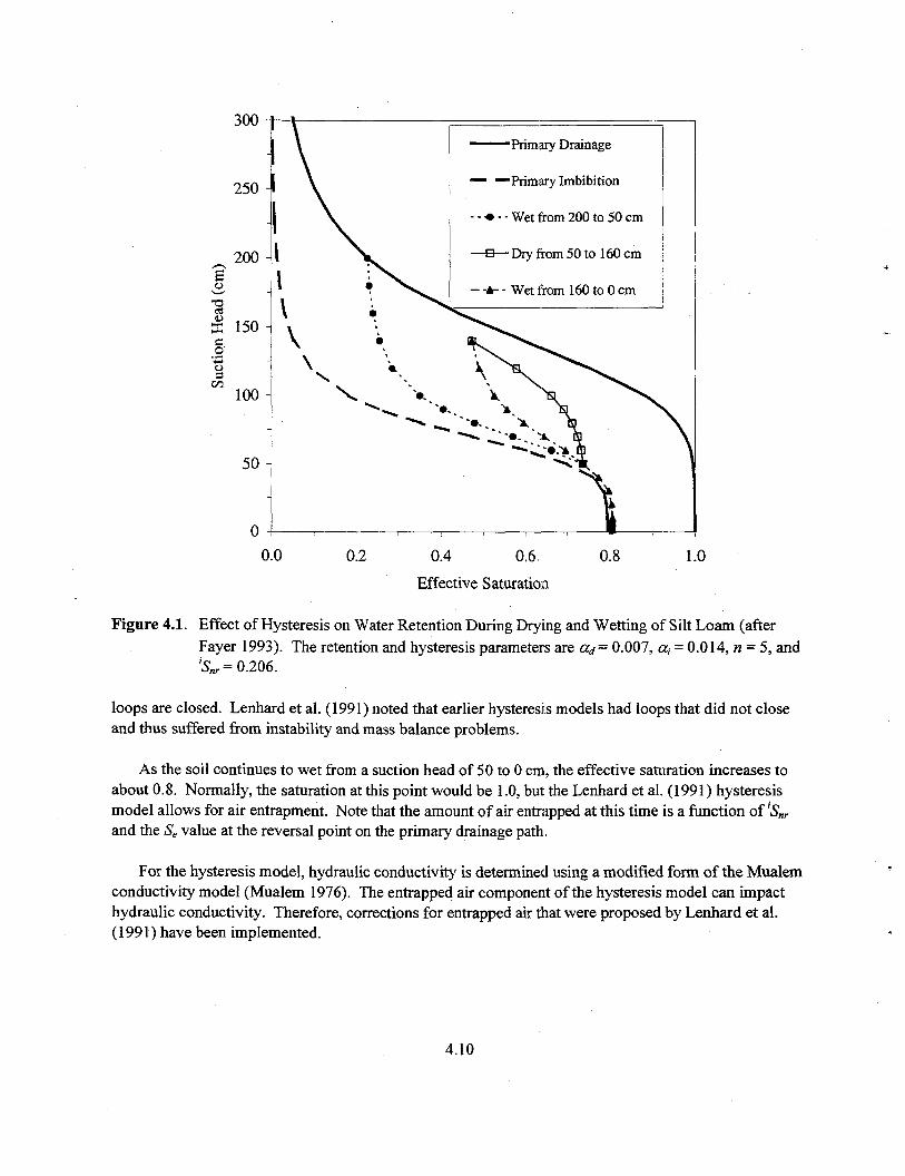
Primary Drainage

Primary Imbibition

Wet from 200 to 50 cm

Dry from 50 to 160 cm

Wet from 160 to 0 cm

0.0 0.2 0.4 0.6.

Effective Saturation

0.8 1.0

Figure 4.1. Effect of Hysteresis on Water Retention During Drying and Wetting of Silt Loam (afterFayer 1993). The retention and hysteresis parameters are aj = 0.007, a, = 0.014, n = 5, and'Snr= 0.206.

loops are closed. Lenhard et al. (1991) noted that earlier hysteresis models had loops that did not closeand thus suffered from instability and mass balance problems.

As the soil continues to wet from a suction head of 50 to 0 cm, the effective saturation increases toabout 0.8. Normally, the saturation at this point would be 1.0, but the Lenhard et al. (1991) hysteresismodel allows for air entrapment. Note that the amount of air entrapped at this time is a function of 'Snr

and the Se value at the reversal point on the primary drainage path.

For the hysteresis model, hydraulic conductivity is determined using a modified form of the Mualemconductivity model (Mualem 1976). The entrapped air component of the hysteresis model can impacthydraulic conductivity. Therefore, corrections for entrapped air that were proposed by Lenhard et al.(1991) have been implemented.

4.10

Modified Brooks-Corey Function. The fifth option uses the modified Brooks-Corey retentionfunction proposed by Fayer and Simmons (1995):

-\/b

K - h > k e (4.32)

The parameter hm represents the suction head at the oven-dry water content (which is zero). Althoughgenerally fixed at 107 cm, the parameter hm may be much higher for very fine-textured porous media andthus could be considered a curve-fitting parameter. In Equation (4.32), the parameter % is defined as

i ln/z .. __.\ (4-33)\nhm

Campbell and Shiozawa (1992) used ^ to describe soil water retention at very high values of suction head,where water retention is essentially an adsorption phenomenon. Their adsorption equation (in a slightlydifferent form) is

e = zea (4.34)

The parameter 6a that occurs in Equations (4.32) and (4.34) is unique to each equation; it is essentially acurve-fitting parameter for the respective equations. The hydraulic conductivity function (not shown,Fayer and Simmons 1995) is based on the Mualem conductivity model.

Modified van Genuchten Function. The sixth option uses the modified van Genuchten retentionfunction proposed by Fayer and Simmons:

hm>h>hc

e=es h<hc

(4.35)

The lower limit of (4.35) is the suction head, hc, at which 0 equals 9S. The value of hc is a function of theother parameters; typical values range from 10"7 to 10"20 cm. The hydraulic conductivity function (notshown, Fayer and Simmons 1995) is based on the Mualem conductivity model.

Rossi-Nimmo Sum Model. The seventh option uses the Rossi and Nimmo (1994) "sum" model todescribe soil water retention. Using their nomenclature, the model is

4.11

h<0

(4.36)°s \no)

0

where ho, hh and X are the curve-fitting parameters. The parameter hd is the suction head at which thewater content is zero (the oven-dry water content). It is equivalent to the parameter hn, used in themodified Brooks-Corey and van Genuchten functions. The two parameters a and c are functions of theother parameters and are calculated internally. The hydraulic conductivity function (not shown, Fayerand Simmons 1995) is based on the Mualem conductivity model.

Rossi-Nimmo Junction Model. The eighth option uses the Rossi and Nimmo (1994) "junction"model to describe soil water retention. Using their nomenclature, the model is

— = 1 /z<0

0 _ f h')2

(4.37)0

6 ' ' ^L j hj<h<hd

where ho and X are the curve-fitting parameters. The four parameters a, c, hh and /?, are functions of theother parameters and are calculated internally. The hydraulic conductivity function (not shown) is basedon the Mualem conductivity model.

4.4.2 Vapor Properties

Doorenbos and Pruitt (1977) provided an empirical equation to calculate saturated vapor pressure as afunction of temperature. The pressure units were millibars. Their equation was modified for UNSAT-Hto provide saturated vapor density in units of g cm'3. The modified empirical equation is

pvs = exp[46.440973- 6 7 9 ° - 4 9 8 5 -6.02808 Inl1 j (4.38)

4.12

The derivative of pvx with respect to temperature is

^ J6790.4985 8U.

4.4.3 Thermal Properties

In Equation (4.22), the thermal conductivity of soil, kh, is a function of water content. Cass et al.(1984) measured values of kh for a soil from the Hanford Site. They used the relationship

6A + B—-(A-D)exp (4.40)

to express kh, J s"1 m"1 K"1, as a function of water content. Cass et al. (1984) also measured the enhance-ment factor [r/ in Equation (4.14)] for the same soil. They then used Equation (4.40) to represent r] as afunction of water content, substituting TJ for kh in Equation (4.40). Equation (4.40) is the only optionavailable in UNSAT-H for describing these two soil properties.

4.5 Evaporation

An equation that integrates the three processes of heat and water flow to the soil surface and transportof water vapor to the atmosphere is an integrated form of Fick's law of diffusion (Campbell 1977)

c_ce\Pvss ~ Pva) (4.41)

/Vv

where e = evaporation flux density, cm hr"1

ce = units conversion factor, cm s m"1 hr"!

/?,..»• = vapor density at soil surface, g cm"3

pva - atmospheric vapor density, g cm"3

rv = boundary layer resistance to vapor transport, s m"1.

Equation (4.41) is an integrated form of Fick's law because it is the result of integrating thedifferential equation form of Fick's law (Equation 4.8) over the atmospheric boundary-layer distance.The result is a vapor density difference divided by a resistance, rather than a diffusivity times a vapordensity gradient. This approach is advantageous in that the thickness of the atmospheric boundary layerdoes not appear explicitly in the equation, but rather is contained implicitly in the resistance term. In itsrepresentation of evaporation, Equation (4.41) does not treat the atmospheric boundary layer as a separateregion by applying the differential form of Fick's law to that region. Instead, the assumption supporting

4.13

Equation (4.41) is that diffusive transport of water vapor in the atmospheric boundary layer is sufficientlyrapid (compared to that in the soil) that a quasi-steady-state water vapor profile exists within the layer,dependent only on p v s s and pva.

Solution of Equation (4.41) requires that the values of three parameters be known. The vapor densityat the soil surface is obtained from the suction head and temperature of the soil surface. The atmosphericwater vapor density is obtained from meteorological data. The third parameter, the atmosphericboundary-layer resistance, is calculated as detailed in Campbell (1985). For bare soil, it is assumed thatthe exchange surface for heat and water are the same (i.e., the soil surface), and that heat and water areexchanged between the soil surface and the atmosphere by the same eddy-diffusion process. Therefore,the atmospheric boundary-layer resistance to water vapor and heat transport is

rv=rh= — ^ hJ hi Yh (4.42)kU

where rv = boundary layer resistance to water vapor transfer, s m'1

rh = boundary layer resistance to heat transfer, s m"1

zT = height of air temperature measurement, md = zero plane displacement, m

zh — roughness height for sensible heat transport, my/h — atmospheric stability correction factor for sensible heat transportk — von Karman's constant

if = friction velocity, m s'1.

The friction velocity in Equation (4.42) is calculated using

U*=-r? —,—-, (4.43)l [ { d ) / \

where u — wind speed, m s"1

zu = height of wind speed measurement, mzm - roughness height for momentum transfer, my/m — atmospheric stability correction factor for momentum transfer.

The atmospheric stability correction factors required for Equations (4.42) and (4.43) are calculateddifferently, depending on the direction of the sensible heat flux (Bussinger 1975; Campbell 1985). Forstable conditions, when the surface temperature is lower than the air temperature and sensible heat flux isfrom the atmosphere to the soil

\j/m=y/h=4.1£ (4.44)

where £"is the atmospheric stability parameter. Atmospheric stability is determined using

4.14

ChaTaU3

(4.45)haTa

where His the sensible heat flux, J m"2 s"1; Cha is the volumetric heat capacity of air, J m'3 K'1; and Ta isthe air temperature, K.

For unstable conditions when the surface temperature is higher than the air temperature and thesensible heat flux is from the soil to the atmosphere, there is a greater potential for eddy diffusion andatmospheric turbulence. For these conditions, the stability correction factors are calculated using

y/h=-2 In1/2

(4.46)

and

(4.47)

Note that the atmospheric boundary-layer resistance (Equation 4.42) depends on the stabilityparameters, which depend on the sensible heat flux, which, in turn, depends on the boundary-layerresistance. Therefore, the atmospheric boundary-layer resistance is calculated using the iterativetechnique described by Campbell (1985).

When heat flow is not being modeled, evaporation is calculated using the Ep concept. The daily Ep isestimated or derived from daily weather parameters (see Section 4.7). As long as the suction head of thesurface node does not exceed the maximum suction head (a value that corresponds to air-dry soil),evaporation will proceed at the Ep rate. When the maximum suction head is exceeded, the simulationcontinues with a constant head boundary in which the suction head of the surface node is equal to themaximum head. For such conditions, the evaporation rate is always less than the Ep rate and is calculatedas the sum of the change in storage of the surface node and the flux between the surface node and thenode below it.

4.6 Transpiration

The mathematical model of transpiration is based on the concept of potential evapotranspiration.Thus, its use is constrained to problems that do not require heat flow to be modeled.

The removal of soil water by transpiring plants is modeled as a sink term in Equation (4.17). Thecalculation of the sink term is accomplished in three steps. First, PET is partitioned into Tp and Ep,subject to the constraint that PET = Ep+Tp. In the second step, Tp is distributed over the root zone inproportion to the relative root density at each depth. This effectively establishes a potential sink term for

4.15

each depth. The final step is to modify the potential sink term of each node, based on water content, toarrive at the actual sink term. Calculation of the sink term in this manner was proposed by Feddes et al.(1978).

Two methods are used to partition PET in the UNSAT-H code. In the first method, Tp is calculatedfrom the leaf area index (/w) using the equation

d<ILA<e (4.48)

with the following parameter values: a = -0.21, b = 0.7, c = 0.5, d= 0.1, and e = 2.7. Equation (4.48) wasdeveloped by Ritchie and Burnett (1971) for cotton and grain sorghum. Ritchie (1972) noted that PET inEquation (4.48) is actually net radiation and not PET in the sense of that calculated by the Penmancombination equation (Doorenbos and Pruitt 1977). Figure 4.2 shows the data and equation from Ritchieand Burnett (1971). Note that Equation (4.48) does not fit the date as well as portrayed by Ritchie andBurnett (1971). Reanalysis of the data resulted in a better set of parameter values: a = 0.0, b = 0.52,c = 0.5, d = 0.0, and e = 3.7.(a) Seasonal ILA data are not currently available for the plant communities atthe Hanford Site; hence, this option has not been tested using Hanford Site data.

1.0

0.8 -

• Ritchie and Burnett data

Ritchie and Burnett Equation

UNSAT-H Version 3.0 Equation

0.0 4-

0.0 0.5 1.0 1.5 2.0

Leaf Area Index

2.5 3.0

Figure 4.2. The Ratio of Potential Transpiration to Potential Evapotranspiration as a Function of LeafArea Index

(a) Personal communication from Mark Ankeny, DB Stephens and Assoc, Albuquerque, New Mexico.

4.16

The second method for partitioning PET uses local cheatgrass data. Hinds (1975) conducted fieldexperiments with cheatgrass growing in microlysimeters in the Fitzner/Eberhardt Arid Lands Ecology(ALE) Reserve of the Hanford Site. During April and May 1972, Hinds measured total and net short-wave radiation, soil heat flux, evaporation, and transpiration; and calculated net long-wave radiation withan empirical equation. Hinds then related transpiration to the total net radiation and computed a ratio thatcould be termed a "crop coefficient." The ratio of transpiration to net radiation applies to the 2 months ofHinds' experiment. The shaded portion of Figure 4.3 represents this ratio for the 2-month period.

According to Klemmedson and Smith (1964), cheatgrass usually germinates in the fall, remainsdormant during the winter, resumes growth in early spring, and flowers and dies of either maturity or lackof soil moisture by early June. To use UNSAT-H to simulate the phenology of cheatgrass, thetranspiration/net radiation relationship (shown as a cross-hatched area in Figure 4.3) has been extendedthroughout the growing season. The code user can do this by choosing two dates. The first date isassigned as the day cheatgrass seeds germinate. The second date is assigned as the day cheatgrass plantscease transpiring because of senescence. Because the dates for these two parameters depend on theconditions of the simulation, they are left as variables for the code user. As seen in Figure 4.3, the ratio oftranspiration to net radiation increases linearly between germination and the first day of maximumtranspiration (day of the year 90), and then decreases linearly from the last day of maximum transpiration(day of the year 151) to zero as the plant senesces.

From year to year, plant biomass production (and thus transpiration) varies because of weather condi-tions and water and nutrient availability. The exact relationship between biomass and transpiration hasnot yet been established for cheatgrass or other common plant species at the Hanford Site. Therefore, anempirical relationship is used to estimate the effect of increased biomass on transpiration. Hinds (1975)

0.4

0.3 -

UNSAT-H Cheatgrass Function

Data Support Period(Hinds 1975)

/

60 120 180

Day of Year

240 300 360

Figure 4.3. Relationship Between the Ratio of Transpiration to Net Radiation and Day of the Year

4.17

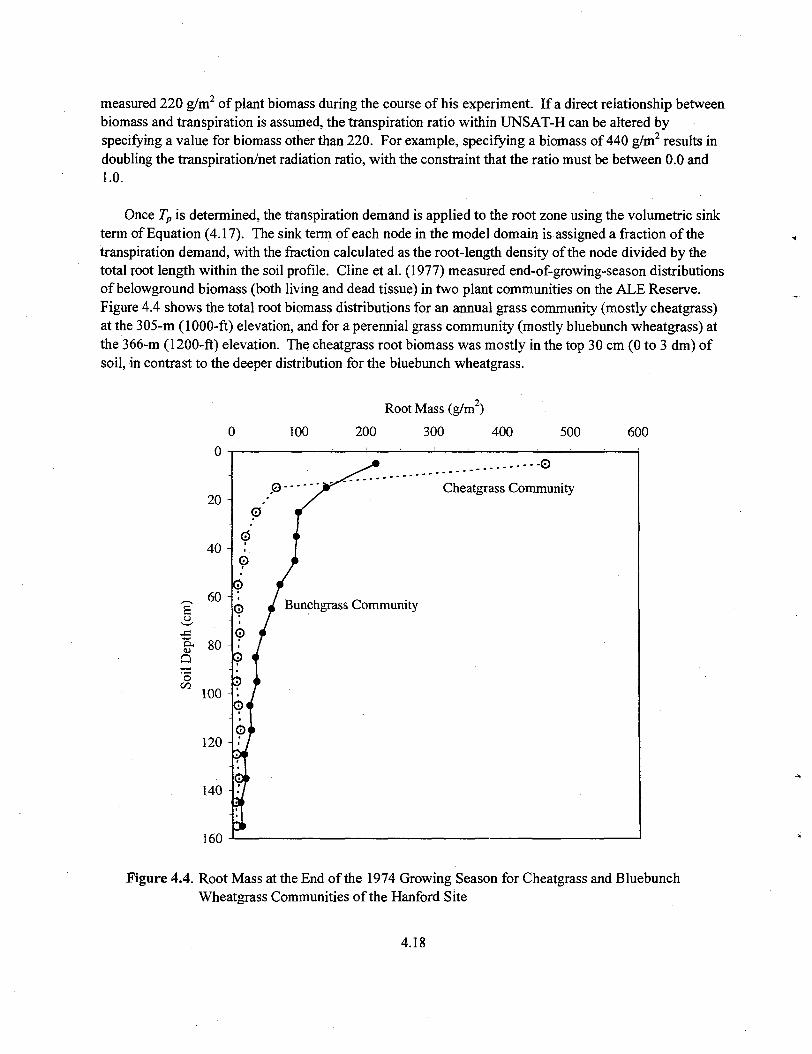
measured 220 g/m2 of plant biomass during the course of his experiment. If a direct relationship betweenbiomass and transpiration is assumed, the transpiration ratio within UNSAT-H can be altered byspecifying a value for biomass other than 220. For example, specifying a biomass of 440 g/m2 results indoubling the transpiration/net radiation ratio, with the constraint that the ratio must be between 0.0 and1.0.

Once Tp is determined, the transpiration demand is applied to the root zone using the volumetric sinkterm of Equation (4.17). The sink term of each node in the model domain is assigned a fraction of thetranspiration demand, with the fraction calculated as the root-length density of the node divided by thetotal root length within the soil profile. Cline et al. (1977) measured end-of-growing-season distributionsof belowground biomass (both living and dead tissue) in two plant communities on the ALE Reserve.Figure 4.4 shows the total root biomass distributions for an annual grass community (mostly cheatgrass)at the 305-m (1000-ft) elevation, and for a perennial grass community (mostly bluebunch wheatgrass) atthe 366-m (1200-ft) elevation. The cheatgrass root biomass was mostly in the top 30 cm (0 to 3 dm) ofsoil, in contrast to the deeper distribution for the bluebunch wheatgrass.

o

oen

20 -

40 -

60 -

80 -

100

120 -

140

160

100

Root Mass (g/m )

200 300 400 500 600

0

Bunchgrass Community

> • 0

Cheatgrass Community

Figure 4.4. Root Mass at the End of the 1974 Growing Season for Cheatgrass and BluebunchWheatgrass Communities of the Hanford Site

4.18

The cheatgrass root biomass data of Figure 4.4 were normalized for biomass found between 0 and80 cm (Table 4.1). Assuming that the normalized total root biomass is directly related to root-lengthdensity {pri), the prL can be related to the depth, z, below the surface by

prL=aexp(-bz) + c (4.49)

where a, b, and c are coefficients that optimize the fit to the normalized bipmass data (a = 1.163,b = 0.129, and c = 0.020). The units of prL are cm roots/cm soil. To calculate the root-density function(pr), the values of prL are multiplied by their respective depth intervals to obtain the total root length.Each prL value is then divided by the total root length to obtain the pr value for each depth. Table 4.1contains the pr values calculated for two depths of root penetration.

After Tp is distributed throughout the root zone, the final step is to calculate the actual transpiration orsink term at each depth. This is done by multiplying the potential sink term, Spo,, of each node by the sinkterm reduction factor, afi a factor that is less than or equal to 1.0 and is a function of the soil water contentof the respective node. The factor prelates the transpiration rate to the water status in the root zone. Therelationship between c^ and water content is shown in Figure 4.5. When the soil water content of a nodeis greater than 6n, c^ equals zero (because anaerobic conditions prevail and the plant ceases withdrawal ofwater from that node). When the soil water content is between Oj and 6», a} is 1.0 and the rate ofwithdrawal is equal to Spol. If the soil water content is between Qw and 6d, the rate of withdrawal isreduced linearly from 1.0 to 0.0 as the water content decreases. When the soil water content is less than6W, Of equals zero to indicate that the plant has stopped withdrawing water from that node.

Table 4.1. Cheatgrass Root-Biomass Data, Root-Length Density (pri), and Root-Density Function (pr)

DepthInterval,

cm

0-10

10-20

20-30

30-40

40-50

50-60

60-70

70-80

Total =

RootBiomass

g/m2

499.4

145.5

51.1

31.5

25.6

15.7

11.8

11.8

792.4

NormalizedBiomass

0.630

0.184

0.065

0.040

0.032

0.020-

0.015

0.015

PrL,

cm roots/cm soil

0.630

0.188

0.066

0.033

0.024

0.021

0.020

0.020

pr (I/cm)

Roots Penetrate to...

80 cm

0.0629

0.0188

0.0066

0.0033

0.0024

0.0021

0.0020

0.0020

20 cm

0.0770

0.0230

—

~

~

~

—

—

4.19

.8

0.0 i

9,Water Content (vol/vol)

Figure 4.5. The Sink Term Reduction Factor aj as a Function of Water Content

4.7 Boundary Conditions

The flow of water and heat across the surface and lower boundary of the soil column of interest isdetermined by boundary condition specifications. Section 4.5 described evaporation (the movement ofwater vapor from the soil surface to the atmosphere). This section describes the remaining boundaryconditions, including liquid water flow; weather variables that affect evaporation, transpiration, and heatflow; heat exchange; and water and heat fluxes at the bottom boundary.

For infiltration events, the upper boundary condition for water flow can be either a flux or constanthead. The flux boundary can be specified as an hourly flux that is equivalent to a precipitation rate. If thesuction head of the surface node should become less than the minimum suction head, the upper boundarybecomes a constant head that is equivalent to the minimum suction head. During this condition,infiltration is calculated as the sum of the change in storage of the surface node and the flux between thesurface node and the node below it. The constant head condition continues until the precipitation ratebecomes less than the potential infiltration rate, and the suction head of the surface node exceeds theminimum suction head. At that time, the upper boundary of the domain reverts to being a flux boundary.The second surface-boundary option is to specify a constant suction head, such as a depth of ponding.The surface water flux then becomes equivalent to the flux between the first and second nodes.

4.20

Similarly, the surface boundary condition during evaporation is either a flux or a constant suctionhead. The input required for the evaporative-flux boundary condition is either daily weather data or dailyPET values. The daily weather data consist of

• daily maximum and minimum air temperatures

• daily average dewpoint temperature

• total daily solar radiation

• average daily wind speed

• daily average cloud cover.

The maximum and minimum air temperatures are used to calculate a sinusoidal variation in airtemperature, Ta, throughout the day, using

Ta=Tmean+Tampcos^{td-l5)\ (4.50)

where Tmean is the average of maximum and minimum air temperatures, K; Tamp is the air temperatureamplitude, R; and td is the time of day, hr. Equation (4.50) assumes the daily minimum temperatureoccurs at 0300 hr and the daily maximum temperature occurs at 1500 hr.

Before 0300 hr, the maximum air temperature from the previous day is used in Equation (4.50). After1500 hr, the minimum air temperature from the next day is used in Equation (4.50). This arrangementensures that air temperature has no discontinuity at midnight.

The dewpoint temperature (and thus the atmospheric vapor density) are assumed to remain constantduring the day. When heat flow is being modeled, solar radiation is distributed during the day as outlinedlater in this section. Wind speed and cloud cover remain constant throughout the day.

When heat flow is not being modeled, the boundary condition for evapotranspiration will be afunction of the PET rate. The PET rate can be either input directly as a daily value or calculated as adaily value using the form of the Penman equation reported by Doorenbos and Pruitt (1977)

(4.51)+ 0.27fl +s + y s + y { 100

where 5 = slope of the saturation vapor pressure-temperature curve, mb K'1

Rni = isothermal net radiation, mm d'1

y = psychrometric constant, mb K"1

U = 24-hr wind run, km d"1

4.21

ea = saturation vapor pressure at the mean air temperature, mbed = actual vapor pressure, mb.

The units used by Doorenbos and Pruitt (1977) were retained for this option.

Whether input or calculated, the PET value is distributed during the day according to the input of thecode user or a sine function. The sine function approximates the daily variation of solar radiation, withthe maximum value occurring at 1200 hr. This option allows 88% of the daily PET to be appliedsinusoidally between 0600 and 1800 hr. During the remaining time, hourly PET rates are 1% of the dailyvalue.

When heat flow is modeled, the surface boundary condition for heat flow can be a calculated heatflux, constant temperature, variable temperature, or constant flux. With the first option, the heat fluxresults from normal exposure of the soil surface to the atmosphere. For this condition, the flux of heatinto or out of the surface node is

G = Rn-H-LE (4.52)

where G = surface heat flux density, J s"1 m 2

Rn = net radiation, J s"1 m'2

H = sensible heat flux density, J s"1 m'2

LE = latent heat flux density, J s"1 m"2.

In Equation (4.52), the net radiation, Rn, is calculated from Campbell (1985) using

Rn ={l-as)St+sacrTa4-ssa-Ts

4 (4.53)

where as = surface albedoS, = solar radiation, J s"! m'2

sa = atmospheric emissivitya = Stephan-Boltzmann constant, J s"1 m"2 K"4

Ta = air temperature, K£•, = soil emissivityTs = soil surface temperature, K.

The calculation of net radiation requires estimates of the surface albedo, the atmospheric and soilemissivities, and solar radiation. Representative estimates of surface albedo are found in Campbell(1977); however, Hillel (1977) concluded that simulating the change in surface albedo during surfacedrying was important. Therefore, the relationship (van Bavel and Hillel 1976)

as= 0.1 + (0.25-0]) (4.54)

4.22

was incorporated in which Oj is the water content at the surface. The albedo value thus calculated isconstrained to between 0.1 and 0.25.

Campbell (1985) recommends that atmospheric emissivity be calculated based on cloud cover. Forclear skies, Campbell recommends the formula of Brutsaert (1975)

sa=A.\lA{Pva)XI1 (4.55)

where pra is the atmospheric vapor density. For cloudy skies, Campbell recommends the formula ofMonteith (1975)

^ac = C1 - 0-84c) sa + 0.84c (4.56)

where sa is the clear-sky emissivity and c is the fractional cloud cover. Under cloudy-sky conditions, Sacreplaces sa in Equation (4.53).

Although the emissivity of the soil surface could be estimated as a constant (Campbell 1977), ss isdependent to some degree on the wetness of the soil surface. Therefore, the relationship (van Bavel andHillel 1976)

^ = 0 . 9 + 0.180! (4.57)

is included in which the emissivity is not allowed to exceed unity.

The daily solar radiation is converted into fluxes that are a function of the time of day. The first stepis to calculate the transmission coefficient, Th which is the ratio of measured solar radiation to potentialsolar radiation. Potential daily solar radiation, Qo, is a function of latitude, <f>, and the solar declinationangle, 8, which varies throughout the year. The potential daily solar radiation is calculated from(Campbell 1985)

Qo = ^ ^ [hs sin(^)sin(£) + cosfo)cos(s)sin(hs)] (4.58)

where hs is cos~'[-tan($tan(<5)]. The sine of the solar declination angle is calculated as

sin(<5) = 0.3985 sin[4.869 + 0.0172 J + 0.03345 sin(6.224 + 0.0172 J)] (4.59)

where J is the day of the year from 1 to 365. The arguments of the trigonometric functions are in radians.If cloud data are unavailable, the fractional cloud cover, c, of Equation (4.56) is that of Campbell (1985)

c = 2.33-3.337; (4.60)

4.23

The value of c is constrained to be within the values of zero and one.

The measured daily solar radiation is converted to fluxes throughout the day using the transmissioncoefficient and

St = SextTt sin(e) (4.61)

where Sex, is the solar constant (i.e., the flux density of solar radiation at the outside edge of the earth'satmosphere on a plane normal to the flux of solar radiation). The last term, sin(e), is the sine of the solarelevation angle, sometimes referred to as the solar altitude. The solar elevation angle is a function oflatitude and time of day and year. The sine of the solar elevation angle is

sin(e)-sin(^)sin(<?) + c o s ^ c o s ^ c o s T — (td -to)\ (4.62)

where td is the hour of the day, and /„ is solar noon, specified in UNSAT-H to be 1200 hr.

The sensible heat flux is the loss or gain of heat by conduction and convection through theatmospheric boundary layer. The equation of choice is an integrated form of Fourier's law of conductionthat closely resembles the integrated form of Fick's law used to calculate evaporation (Equation 4.41)

H = ̂ -{TS-Ta) (4.63)

In a manner similar to that of the evaporation model, Equation (4.63) is used to represent the sensibleheat flux such that the atmospheric boundary layer is not treated as a separate region in which thedifferential form of Fourier's law applies. Rather, Equation (4.63) assumes that the heat flux across theboundary layer is sufficiently rapid (compared to that in the soil) that a quasi-steady-state temperatureprofile exists within the layer and is dependent only on Ts and Ta.

The latent heat term in Equation (4.52) is the product of the latent heat of vaporization, L, and theevaporation rate, E. The evaporation rate is calculated from Equation (4.41). Using Equations (4.53),(4.63), and (4.41), heat flux, G, at the soil surface can be calculated using Equation (4.52).

When the surface boundary condition for heat flow is constant temperature, the heat flux at thesurface is equated to the heat flux between the surface node and the node below it. When the surfacetemperature is allowed to vary sinusoidally during the course of a day, the heat flux at the surface isequivalent to the flux between the surface node and the node below it, plus the change in heat storage atthe surface node. For the last option, a constant heat flux is specified.

The second boundary to be specified is the lower boundary. The four options for flow of water acrossthis boundary are 1) unit gradient, 2) constant suction head, 3) specified daily flux, and 4) impermeableboundary (i.e., zero flux). The unit gradient option corresponds to gravity-induced drainage and is most

4.24

appropriate when applied to soil profiles that extend below the root zone and in which drainage is notimpeded. With the unit gradient condition, the calculated drainage flux depends on the liquid waterconductivity of the lower boundary node. The constant suction head option is most often chosen whenthe soil profile being simulated extends to a static water table, in which case the constant suction headvalue would be zero. Whenever drainage fluxes are known, they can be input directly using the fluxoption. Finally, the impermeable lower boundary condition can be used when drainage is restricted (e.g.,in closed-bottom lysimeters).

For heat flow, the three options for the lower boundary condition are 1) constant gradient, 2) constanttemperature, and 3) constant flux. For the constant gradient option, the heat flux across the lowerboundary is a function of the chosen gradient, the thermal conductivity of the lower boundary node, andthe thermally induced vapor flux. For the constant temperature option, the heat flux across the lowerboundary is equal to the flux between the lower boundary node and the node above it. For the thirdoption, a constant heat flux is specified. A value of zero can be used to model a boundary impermeable toheat flow.

4.25

5.0 Numerical Implementation

The equations used to represent the conceptual model are solved numerically with a Crank-Nicholsonfinite difference scheme. In this scheme, the mathematical equations are approximated with finitedifference equations in which a finite grid represents both the space and time derivatives. Some error isassociated with this approximation, but the error can be minimized by decreasing the size of the spaceand/or time grid intervals. The finite difference equations can be formed into a matrix that is amenable toan iterative solution scheme using either standard or modified Picard iteration (Celia et al. 1990).

A new feature of UNSAT-H Version 3.0 is the strategy of solving for suction head and temperature inalternating steps while iterating a time step. This strategy represents a departure from the strategy used inVersion 2.0, in which the suction head solution was obtained first, followed by the temperature solution.The new strategy of alternating the suction head and temperature solution per iteration produces muchmore stable results.

5.1 Finite Difference Approximation of Water Flow

With the Crank-Nicholson method, the time derivatives are evaluated at the midpoint of the time step.Thus, Equation (4.17) is approximated in the computer code as

rj-\l2hi-hr _ -2 [ ,-1/2 ;-l/2l <w-l/2 ( , n

where

and

t+l/2 +1j±\/ sr

The subscript / denotes the node at depth z,-. The superscript^ denotes the time, tj, for which the solutionwill be determined. The sink term, Si, is directly calculated in the code as a function of the time of dayand the water content, e/~V2.

The flux terms at the midpoints between nodes are approximated by

5.1

L,i+\/2 " A vr , i+ l /2I TV — T-J

zi+\ zi(5.4)

and

^i-\/2~KT,i-l/2\ zi~zi-\GKL,i-\I2 ~KvT,i-\l2 zi~zi-\

(5.5)

During the first iteration of the water flow calculation, soil temperatures T/ are equivalent to T/~l •

During subsequent iterations, soil temperatures T/ are set to their values at the end of the previous

successful iteration.

The G term in Equations (5.4) and (5.5) is the gravity flow factor. When G has a value of 0, thegravity inducement to flow is neglected, thus allowing for simulation of horizontal flow. When G is 1,the gravity inducement to flow is included.

In Equations (5.4) and (5.5), the hydraulic conductivity between nodes can be calculated as thearithmetic mean (with an option for weighting the arithmetic mean to the upstream or downstream flowdirection), the harmonic mean, or the geometric mean. The arithmetic equation is

(5.6)

where (ov and coj represent upstream and downstream weighting options, with the constraint that cou += 1. The equations for the harmonic and geometric means are

1 1j (5.7)

(5.8)

Values of KL are calculated from the input soil properties based on the head value of the correspondingnode.

The isothermal vapor conductivity, Kvh, [which is part of KT in Equations (5.4) and (5.5)] is calculatedaccording to

5.2

aDaMgP£<

pexp

-hJMg

RTtj~l

(5.9)

based on Equations (4.9), (4.13), and (4.15). The value ofKv/, for the midpoint is calculated in the samemanner as the liquid conductivity at the midpoint [i.e., using equations similar to Equations (5.6), (5.7),and 5.8)]. In Equations (5.4) and (5.5), the total conductivity applicable to a suction head gradient at amidpoint is thus

J — vi7\i+l/2 ~ AZ,/+l/2

The thermal vapor conductivity, KrT, is calculated according to

(5.10)

aDn_rz_s. exp-hJMg

BltX dT/7-1(5.11)

based on Equations (4.9), (4.13), and (4.16). The value of AV at the midpoint between nodes is calculatedusing the equally weighted arithmetic mean [Equation (5.6)].

5.1.1 Interior Nodes

Equation (5.1) is rearranged to solve for the suction head values at the end of a time step, with thegeneral form of the rearranged equation being

(5.12)

For the boundary nodes, the exact form of the coefficients in Equation (5.12) depends on the boundaryconditions chosen. For all interior nodes, however, the coefficients for nodes i = 2,n-l are

A- (5.13)

j-l/2Bi ~T~

KT,i+\l2 r,;-l/2 (5.14)

5.3

r* _ KT,i+li2(5.15)

(5.16)

When the modified Picard iteration technique is used, the B and D coefficients are modified. For

B , the capacity in Equation (5.14) is changed from C{~ to C{ . For D , the entire term containing

the capacity is replaced. The modification is

Cj~XI2hj~X 9j~X -0J'm +CJ'mhj'm- n u ' i . ' ' ' ' (5.17)

where the superscript u signifies the unmodified coefficient calculated in Equation (5.16), and thesuperscript m is an iteration counter. Iteration m represents the last completed iteration, while iterationm+\ represents the current iteration.

5.1.2 Surface Boundary Node

By convention, the surface boundary node in UNSAT-H is node 1. The values of coefficientsassigned to node 1 will depend on which surface boundary condition is chosen. One option in UNSAT-His to specify a constant suction head for node 1. The resulting solution equation for node 2 (the nodebelow node 1) is

(5.18)

5.4

In this case, the number of equations in the solution matrix is reduced by one because h} is alreadyknown.

Another surface boundary option in UNSAT-H specifies a surface flux, either as evaporation orprecipitation. The special form of Equation (5.12) for this case looks like

(5.19)

where

(5.20)

*r=- (5.21)

C =•T,3/2 (5.22)

M/2,/-ID =

CJ~l/IhJ

y-1

r,3/2V

••vr,3/2

V

(5.23)

Note that plant water withdrawal from the surface node is not allowed. Also, the surface flux, qj~jl2, is

either specified by the user or calculated directly (e.g., the evaporative flux). The program checks duringeach time step to determine if the head value at the soil surface exceeds the range of values permitted(being either too wet or dry). If it does, then the suction head at the surface boundary is reset to theappropriate limit and the problem is re-solved for that time step for the remaining nodes. At the start ofthe next time step, the program will again assume a surface flux condition.

When evaporation and heat flow are simulated, the evaporation rate is calculated usingEquation (4.41):

5.5

0 \Pvss + Pvss } ~ Pva

7-1/2(5.24)

The negative sign was added to the beginning of Equation (5.24) to align the evaporation rate with theUNSAT-H convention that positive flux is downward.

The evaporation rate depends on pvss, which is the product of the saturated vapor density at the soilsurface temperature and the relative humidity (Equation 4.13) at the soil surface. Because of thedependence of e on pYSS, the evaporation rate is a nonlinear function of the suction head, h\, of the surfacenode. A fraction of the dependence of e on h\ can be represented by expanding the exponential in

Equation (4.13) and moving the linear hi term to the left-hand side of the matrix by modifying £j and

.D] . The identity used to expand the exponential is

exp

where

(5.25)

(5.26)

The modifications to the coefficients are

(5.27)

ce pvsh(Mg(5-28)

where B\u and D\u on the right-hand side represent the unmodified version calculated previously.

When the modified Picard iteration technique is used, the B and D coefficients are modified. For

B , the capacity in Equation (5.14) is changed from C{~ to C( . For D*, the entire term containing

the capacity is replaced. The modification is

5.6

D*x = £>,** l- L— + — - —•r—~— (5-29)

where the superscript u signifies the unmodified coefficient calculated in Equation (5.16), and thesuperscript m is an iteration counter. Iteration m represents the last completed iteration, while iterationm+\ represents the current iteration.

5.1.3 Lower Boundary Node

Of the four options for determining the lower boundary condition, one is a fixed suction-head option.For this option, the user specifies in the initial conditions what the suction-head value of the node will be.The solution equation for node n-1 changes to

and the number of equations to be solved is reduced by one. The user can specify a constant water tablecondition by using this fixed suction-head option and setting hn to zero.

The three other options are flux options. The general form of Equation (5.12) that is pertinent to allthree options is

*4h>H_l+B*nhl = D*n (5.31)

where

* KT,n-\l2 , , - - .An • — (5.32)

\zn-zn-\)

R* _ ° « 1 ,n-\lI ,r „>

tj-tj l{zn-zn_xy

C*n=0 (5 .34)

5.7

J-xl2hj-x

tJ -tJ

(zn-zn-l)

v7>-l/2

V

(5.35)

For the impermeable boundary option, the time-averaged flux, qi'V.l, is set equal to zero. For the

specified flux boundary, q-^'lii is set equal to values specified by the code user. For the unit-gradient

boundary condition, the flux is calculated as

(5.36)

When the modified Picard iteration technique is used, the B and D coefficients are modified. For

B*, the capacity in Equation (5.14) is changed from C^""1/2 to CJn . For D*, the entire term containing

the capacity is replaced. The modification is

p.* _un -

cj,mhj,m

• ;

tJ -tJ(5,37)

where the superscript u signifies the unmodified coefficient calculated in Equation (5.16), and thesuperscript m is an iteration counter. Iteration m represents the last completed iteration, while iterationm+l represents the current iteration.

5.1.4 Mass Balance Error

The first step in calculating the mass balance error is to calculate the soil-water storage at the end of atime step using

(5.38)

Then, the mass balance error (Ew) for the time step can be obtained using

F — JJ — (5.39)

5.8

where the terms V, EJ' ,TJ', D^ and {s^-S^, 1 j refer to the amounts of infiltration, evaporation,transpiration, drainage, and change in storage, respectively, that have occurred during the time step.

5.2 Finite Difference Approximation of Heat Flow

In the Crank-Nicholson method, the time derivatives are evaluated at the midpoint of the time step.Thus, Equation (4.22) is approximated in the computer code as

CJ~hi-1/2 -1/2

- 2zi+\ ~zi-\

U-l/2 __y-l/2 1PA.j+1/2 *A,/-l/2j

where

/ -I

hwJ [tJ-fj- i(5.40)

(5.41)

j-\ 12 _ J_ L Ly y, \ L;-i

-To (5.42)

(5.43)

and

~ $ h (ih,i±\l2 (5-44)

The subscript i denotes the node at depth z,. The superscript^ denotes the time, tj, for which the equationsare solved.

The flux terms at the midpoints between nodes are approximated by

h,i+l/2V

J T

(5.45)

1 T

5.9

and

h,i-\I2 zi~zi-\ ,\ J

Lo + Ckv_[ i—l f

(5.46)

ckw -T

The thermal conductivity values in Equations (5.45) and (5.46) are calculated using an arithmetic mean.The qv term in Equations (5.45) and (5.46) is the sum of qv/, and qvT, and is obtained from solution of thewater flow equation. Both qi and qv are updated with each iteration.

5.2.1 Interior Nodes

Equation (5.40) is rearranged to solve for the temperature values at the end of a particular time step,with the general form of the rearranged equation being

Al Li-\ + t i l i i + *-l J-i+l - ul (5.47)

For the boundary nodes, the exact form of the coefficients in Equation (5.47) depends on the boundaryconditions chosen. For all interior nodes, however, the coefficients for nodes i = 2,n-\ are

4-=-~ zi-\

-!rJ'Kh,i-\12

zi~zi-\

£hv_ j-1/2 _£hw_ j-1/22 qv,i-M2 2 qL,i-M2 (5.48)

rj-\l21

tJ -tJ~l Zf+l-Zi-l

Kh,i+M2

zi+\ ~zi\ J

Kh,i-V2zi ~ zi-\

V J

'hvJ~l/2

1 ^ _ + _JLzi+\ ~ zi-\

'hw

zt+\ - zi-\

(5.49)

zi+\ ~

'^h,i+\/2

zi+\~zi

£hv_ j-l/2 + £hw ^j-1q

J

(5.50)

5.10

A*=-^f -kJ~i-izi+\ ~ zi

Kh,i-\I2

L0+Chv\T-^-T0

(T(Lo -

0J--0J~~l

zi+\ ~ zi-\ r/:1l~l T

'hw -rA?Ld£

Zi+\ ~ Zi-\

'hw

/ - i

— Tn,7-1/2

r ,-_i ,-_i \ '

i ~ zi-\

1 T1 n

— T

-C, T

(5.51)

5.2.2 Surface Boundary Node

The values of the coefficients assigned to node 1 (the surface node) depend on the option chosen forthe surface boundary condition for heat flow. Two of these options in UNSAT-H Version 2.0 permitspecification of either a constant or variable temperature for node 1. The resulting equation for heat flowat node 2 (the node below node 1) is

(5.52)

In this case, the number of equations in the solution matrix is reduced by one because Ti is alreadyknown.

The remaining two options for the surface boundary condition for heat flow in UNSAT-H are to treatthe surface boundary as a heat flux. The special form of Equation (5.47) for this option looks like

(5.53)

(5.54)

5.11

,--1/2* ^h,\ , "-̂ ,3/2

Chv

{z2-zl f

{

z2-zx

(5.55)

- i * •

- I = •Chv (5.56)

A =--t

j~X A,3/2

/-I

-2q y-1/2

-

1

^ 2 -

V

z\

T/- l / - I

,7-1/2 + Chv • - T7-1/2

<3/2

V Jtj -tJ~l

l --T

v

(5.57)

hwIo\^L,3/2

According to the option chosen, the time-averaged flux, qh, across the soil surface can be calculated[using Equation (4.52)] as a function of weather and soil parameters, or specified by the code user. Whenevaporation occurs, qv\ < 0 and qL,\ = 0. When precipitation occurs, qv\ = 0 and qi\ > 0.

5.12

5.2.3 Lower Boundary Node

Of the three options for determining the lower boundary condition, one is a constant temperatureoption. For this option, the user specifies in the initial conditions what the temperature value of the nodewill be. The solution equation for node w-1 changes to

(5.58)

and the number of equations to be solved is reduced by one.

The two other options are flux options. The general form of Equation (5.47) pertinent to these twooptions is

(5.59)

where

1

fj -t

chv2

Chw2

tj

^-

kh,n-\l2 Ckv j-i/2 Chw J-H2

Kh,n-\I2

- / • ' zn ~' zn-\

-tj~l zn-zn-\

(5.60)

(5.61)

(5.62)

5.13

j-Mlrpj-X

(zn-Zn-\)

n in-\

TJ -1

'hv\ft T"7

a] _°vnv,n

2TJ +VTn 7T J-l/2

/ • 1 -1

Lo +chv\ r 10

/-1/2

T

°

(5.63)

ln

12 -chw

j-l/2 j-l/2

,n-\/2

One of the two heat flux options for the lower boundary condition is a specified temperature gradient( PTM). For this option, the flux is calculated as

(5.64)

If vapor flow is included, the temperature gradient at the bottom of the domain can induce a thermalvapor flux, represented by the second term on the right of Equation (4.14). The second flux optionspecifies a constant heat flux. With this option, the heat flux can be set equal to zero to simulate aboundary impermeable to heat flow. A thermally induced vapor flux across the bottom boundary is notpermitted with this second heat flux option.

5.2.4 Heat Balance Error

Once a temperature solution has been obtained, a heat balance error (Eh) is calculated. First, the heatstorage (51/,) of the soil during the time step is calculated using

5.14

+\L +C1.T \\9J -9J' 1+C1. T \9J -9J \ (5 651

+(L0

z=2L x

where

ATi^T/-T/~l (5.66)

r0 (5.67)

Then, the heat balance error for the time step can be obtained using

. / , , , \

where the terms Rn, LE, H, QHn, and \SJh - Sj^ J refer to the net radiation, latent heat, sensible heat,

lower-boundary heat flows, and change in heat storage that have occurred during the time stepy. The

calculated EJh value is an informative index of the heat flow calculations and does not affect the

calculation of water or heat flow or the time-step size. Individual E}h values are summed during each

output cycle.

5.3 Time Steps

Time steps must be kept small to solve the system of nonlinear equations with a minimum of errorassociated with the time discretization.. Ideally, the optimal size of the time steps would be infmitesimallysmall. Practically, however, their size must be sufficiently large that a solution can be reached in areasonable amount of computer time. In UNSAT-H, the time step is allowed to vary between specifiedminimum and maximum values. Within this range, the size of the time step will vary depending on user-defined criteria. Each criterion is evaluated relative to a user-defined acceptable value. If greater, thetime step is reduced. If less, then the time step size is increased. The degree of decrease or increase isrelated to the size of the difference from the acceptable value.

A total of five criteria are available for controlling the size of the time step. Two of these criteria are

the maximum relative change in water content \A9rei) defined as

5.15

A6rd = MAX e{-e{-er

(5.69)

and the mass balance error defined by Equation (5.39). One of these two criteria must be chosen, but theycannot be used simultaneously. The selected criterion is evaluated at the end of each time step.

The remaining three criteria are optional. The first optional criterion is to use the maximum relative

change in suction head {£hrei) defined as

= MAXhZ-h/-1

(5.70)

The second optional criteria is to monitor the maximum change in suction head, defined as

? -hj'1 (5.71)

In both cases, the criterion is evaluated at the end of each iteration within a time step. The third optionalcriterion is to use the heat balance error defined by Equation (5.68). This criterion is evaluated at the endof a time step.

At the start of a simulation, the time step size is set to the minimum size. Thereafter, the time stepsize is governed by the time step criteria invoked. The only exception occurs at the start of an infiltrationevent, when the time step size is automatically reduced by a user-defined factor.

During simulations, time step adjustments are carried out as follows. After solving the water and heat(if necessary) flow equations to determine the matric suction and temperature solutions, the chosencriteria are calculated and compared to the allowable limits. If any of the limits are exceeded, the matricsuction and temperature solutions are rejected, the time step is reduced by a factor between 0.5 and 1.0(depending on the degree to which the criterion exceeds the assigned limit), the coefficient matrix isrecalculated, and new solutions obtained. This process continues until either the criteria are within theallowable limits or the time step is reduced to the minimum allowable value. If an acceptable solution isnot obtainable using the minimum time step, the program will terminate with an error message.

When all of the criteria are within the allowable limits, the next time step size is increased relative tothe one just completed. The size of each successive time step can be increased until the maximumallowable time step, as defined by the user, is reached. From then on, as long as the criteria are satisfied,the time step size will be set to the maximum value.

5.16

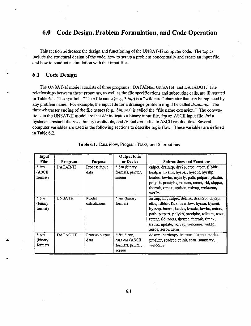
6.0 Code Design, Problem Formulation, and Code Operation

This section addresses the design and functioning of the UNSAT-H computer code. The topicsinclude the structural design of the code, how to set up a problem conceptually and create an input file,and how to conduct a simulation with that input file.

6.1 Code Design

The UNSAT-H model consists of three programs: DATAINH, UNSATH, and DATAOUT. Therelationships between these programs, as well as the file specifications and subroutine calls, are illustratedin Table 6.1. The symbol "*" in a file name (e.g., *.inp) is a "wildcard" character that can be replaced byany problem name. For example, the input file for a drainage problem might be called drainAnp. Thethree-character ending of the file names (e.g., bin, res) is called the "file name extension." The conven-tions in the UNSAT-H model are that bin indicates a binary input file, inp an ASCII input file, hri ahysteresis restart file, res a binary results file, and Us and out indicate ASCII results files. Severalcomputer variables are used in the following sections to describe logic flow. These variables are definedin Table 6.2.

Table 6.1. Data Flow, Program Tasks, and Subroutines

InputFiles

* .inp(ASCIIformat)

*.bin(binaryformat)

*.res(binaryformat)

ProgramDATAINH

UNSATH

DATAOUT

PurposeProcess inputdata

Modelcalculations

Process outputdata

Output Filesor Device

*.bin (binaryformat), printer,screen

*.res (binaryformat)

*.lis, * .out,toss, out (ASCIIformat), printer,screen

Subroutines and Functionscalpet, drain2p, dry2p, etbc, etpar, filbldr,heatpar, hysini, hyspar, hysout, hysshp,kcalcs, lowbc, myhrly, path, petpart, plantin,polykh, precipbc, relhum, retent, rid, shppar,thermk, timex, update, volvap, welcome,wet2pairtmp, blr, calpet, delchk, drain2p, dry2p,etbc, filbldr, flux, heatflow, hysini, hysout,hysshp, interk, kcalcs, kvcalc, lowbc, netrad,path, petpart, polykh, precipbc, relhum, reset,retent, rid, roots, therme, thermk, timex,trsink, update, volvap, welcome, wet2p,zeroa, zeroi, zerorddsum, hardcopy, initsum, listdata, nodez,profiler, readrec, reinit, scan, summary,welcome

6.1

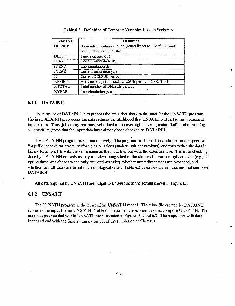
Table 6.2. Definition of Computer Variables Used in Section 6

VariableDELSUB

DELTIDAYIDENDIYEARNNPRINTNTOTALNYEAR

DefinitionSub-daily calculation period; generally set to 1 hr if PET andprecipitation are simulated.Time step size (hr)Current simulation dayLast simulation dayCurrent simulation yearCurrent DELSUB periodActivates output for each DELSUB period if NPRINT=1Total number of DELSUB periodsLast simulation year

6.1.1 DATAINH

The purpose of DATAINH is to process the input data that are destined for the UNSATH program.Having DATAINH preprocess the data reduces the likelihood that UNSATH will fail to run because ofinput errors. Thus, jobs (program runs) submitted to run overnight have a greater likelihood of runningsuccessfully, given that the input data have already been checked by DATAINH.

The DATAINH program is run interactively. The program reads the data contained in the specified*.inp file, checks for errors, performs calculations (such as unit conversions), and then writes the data inbinary form to a file with the same name as the input file, but with the extension bin. The error checkingdone by DATATNH consists mostly of determining whether the choices for various options exist (e.g., ifoption three was chosen when only two options exist), whether array dimensions are exceeded, andwhether rainfall dates are listed in chronological order. Table 6.3 describes the subroutines that composeDATAINH.

All data required by UNSATH are output to a *.bin file in the format shown in Figure 6.1.

6.1.2 UNSATH

The UNSATH program is the heart of the UNSAT-H model. The *.bin file created by DATAINHserves as the input file for UNSATH. Table 6.4 describes the subroutines that compose UNSAT-H. Themajor steps executed within UNSATH are illustrated in Figures 6.2 and 6.3. The steps start with datainput and end with the final summary output of the simulation to file *.res.

6.2

Table 6.3. Subroutines in DATAINH

Name Purposecalpet.f Calculates PET using the Penman equation

datainhf Severs as the main program of DATAINHdrain2p.f Calculates the apparent water saturation, entrapped air saturation, permeability, and apparent

saturation capacity for the primary drainage path with and without air entrapmentdry2p.f Calculates water and air saturations, relative permeability, and capacity for drainage pathsetbc.f Reads in the PET and meteorological boundary conditionsetpar.f Reads in PET and meteorological parametersfilbldr.f Reads in list of filenames containing PET, meteorological, and precipitation dataheatpar.f Reads the soil parameters for heat flowhysini.f Initializes variables for the hysteresis codehysout.f Outputs final hysteresis variables from UNSAT-H to an external file for use in a possible restarthyspar/ Reads soil parameters for hysteresishysshp.f Passes the UNSAT-H parameters into the hysteresis routines in the correct units and converts the

output to UNSAT-H unitskcalcs.f Calculates hydraulic properties specific to modified Brooks-Corey and Van Genuchten functionslowbc.f Reads in the lower boundary conditionsmyhrlyf Calculates hourly distribution of PET based on the sine wave approach

path/ Calculates the air-water capillary head, the amount of entrapped air, and the water saturation usingthe input pressure heads of water and air

petpartf Partitions PET into potential transpiration and evaporationplantin./ Reads in plant parameterspolykh.f Calculates the conductivity of each node as a function of the suction head valueprecipbc.f Reads in precipitation data and writes meteorological and precipitation data to binary input filerelhum.f Calculates the relative humidity using suction head and temperatureretent.f Calculates the water content and moisture capacity of each node as a function of the suction head

valuerld.f Calculates root density as a function of depthshppar.f Reads in soil hydraulic property parametersthermkf Calculates soil thermal conductivity and volumetric heat capacitytimex.f Queries the operating system and returns the time and dateupdate./ Resets global variables after successful solution, and checks the index variables and sets them to

the proper saturation pathCalculates volumetric vapor contentvolvap.fWrites program header with version number and contact personCalculates water and entrapped air saturations, relative permeability, and capacity for wetting paths

welcome./wet2p/

6.3

WRITE (LUB) DV, I PLANT, LOWER, NDAYS,NDAY,NPRINT,ITOPBC,ICONVH, MAT, && KOPT, KEST, IVAPOR, IDEND, IFDEND,NYEARS, IYS, ISWDIF, ICLOUD, && NPT,G,MAXPOL,MAXCOE,IEVOPT,NFPET,NSOW,NHRVST,IDTEND, && INC,MXROOT,IETOPT,ISHOPT,INMAX, ISTEAD,ILEAP, && IRAIN, IHEAT,UPPERH,LOWERH,IFILE, HYFILE,TITLEWRITE(LUB) DMAXBA,DELMAX,DELMIN,RAINIF,RFACT,HIRRI,HDRY,SATK, &

& DRYK,SATC,DRYC,SATTH,DRYTH,AA,B1,B2,TMOIST,LOG10E, && DHMAX,DHFACT,QHCTOP,OUTTIM,DMAXHE,HTOP,TGRAD,UP,DOWN, && STOPHR,GRAV,TSMEAN,TSAMP,DLAI,BAREWRITE(LUB) (Z(I) ,H(I),NTROOT(I),THETA(I) ,KL(I) ,C(I),T(I), &

& CHSOIL(I),I=1,NPT),THETAW,THETAD,THETAN,RDF,FPET, && MGR,VAPDIF,VC,TSOIL,PETPC,QWLEAK,QHLEAKWRITE(LUB) SWPA,SHPA,SINLAT,COSLAT, TANLAT, TPIY, DAYSEXT,SB,CHW, &

& ALBEDO,ALT,PMB,ZU,ZH,ZM,ZT,D,VK,SEXT,CHA, && TCON,CHS,EF,WATDEN,LHV0,CHV, . && T0,HSTORE,ISMETH,DHTOL,RHA,IHYS, HYSHPH,SARWA,IPATHA, S& AIRTOL, HYSTOL,HYSMXH,INDEXB,BBHEAD,HM,THTA,ALFACTWRITE(LUB) (PMFN(I),I=1,NYEARS)WRITE(LUB) (PRFN(I) ,I=1,NYEARS)WRITE(LUB) PTRANS, PEVAPOWRITE(LULO) NWATERIF (ET_OPT .EQ. 0) THEN

IF (I .EQ. IRDAY) WRITE(LULO) IRDAY,IRTYPE,EFICEN,NP, && (RTIME(J),AMOUNT(J),J=1,NP)ELSE

WRITE(LULO) METDAY, (RMDATA(J,I) , J=2,7) , IRTYPE, EFICEN,NP, && (RTIME(J),AMOUNT(J),J=1,NP)ENDIF

Figure 6.1. Format of the *:bin File Created by DATAINH for Input to UNSATH. LUB is thelogical unit name for the binary output file. LULO is an alternate unit name that isequivalent to LUB.

Simulation data that are output to the *.res file include initial conditions, DELSUB and day-endvalues for head, water content, water and heat flow, temperatures, plant-sink terms, water and heat-balance terms, and at the end of the file, the simulation end results. The *.res format is shown inFigure 6.4.

6.1.3 DATAOUT

The purpose of DATAOUT is to process the UNSATH output data. Specifically, DATAOUTconverts the binary output data found in a *.res file into ASCII format so that the results can be sent toeither a screen for viewing or a printer or file for permanent record. Table 6.5 describes the subroutinesthat compose DATAOUT.

6.4

Table 6.4. Subroutines in UNSATH

Nameairtmp.fblr.fcalpet.fdelckkfdrain2p.f

dry2p.fetbc.f

flux./hdrycalc.f

heat/low./hysini.fhysout.fhysshp.f

interk.fkcalcs.fkvcalc.fnetradf

path/

petpart.f

polykhfpfecipbc.frelhum.freset./

retent.f

rid./roots./therme./ihermk./timex./tridag.ftrsink./unsath./update./

volvap./

PurposeCalculates the air temperature as a function of time of dayCalculates the boundary layer resistance to heat and vaporCalculates PET using the Penman EquationAdjusts the time step according to the mass and heat balance errorsCalculates the apparent water saturation, entrapped air saturation, permeability, and apparentsaturation capacity for the primary drainage path with and without air entrapmentCalculates water and air saturations, relative permeability, and capacity for drainage pathsReads in the PET and meteorological boundary conditionsCalculates liquid and vapor water fluxes between nodesCalculates a value for HDRY based on the temperature of the soil surface and the relativehumidity of the atmosphereSolves the heat balance equationsInitializes variables for the hysteresis codeOutputs hysteresis variables from UNSAT-H to an external filePasses the UNSAT-H parameters into the hysteresis routines in the correct units and converts theoutput to UNSAT-H unitsCalculates internodal liquid, vapor, and heat conductivitiesCalculates hydraulic properties specific to modified Brooks-Corey and Van Genuchten functionsCalculates vapor conductivitiesCalculates net radiation as a function of latitude, time of year, time of day, air and surfacetemperature, atmospheric vapor density, albedo, cloud cover, surface and air emissivities, andextraterrestrial solar fluxCalculates the air-water capillary head, the amount of entrapped air, and the water saturation usingthe input suction heads of water and airPartitions PET into potential transpiration and evaporationCalculates the conductivity of each node as a function of the suction head valueReads in precipitation data and write meteorological and precipitation data to binary input fileCalculates the relative humidity using suction head and temperatureCopies R values into A to a) initialize parameters at start of iteration loop, and b) reset parametersafter a time step reductionCalculates the water content and moisture capacity of each node as a function of the suction headvalueCalculates root density as a function of depthCalculates maximum rooting depth and the root-density functionCalculates enhancement factor for soil vapor flow caused by thermal gradientsCalculates soil thermal conductivity and vol. heat capacityQueries the operating system and returns the time and dateSolves the tridiagonal solution matrixCalculates the sink term at each node, and sums the sink terms to get transpirationServes as the main program of UNSATHResets global variables after successful solution, and checks the index variables and sets them tothe proper saturation pathCalculates volumetric vapor content

6.5

Table 6.4. (contd)

Namewelcome./wet2p.fzeroa.fzeroLfzeror.f

PurposeWrites program header with version number and contact personCalculates water and entrapped air saturations, relative permeability, and capacity for wetting pathsSets ARRAY variables to zeroSets INTEGER variables to zeroSets REAL variables to zero

Read ".bin File7 /write Initial 7

/ — • / Conditions f—>-j I to \res File /

Initializationof Variables IYEAR>NYEARS

Write YearlySummary

to *.res File

InitializeDaily

Variables

InitializeYearly

VariablesI DAY >IDEM)

WriteDaily Summary

to '.res File

Update Yearly

UpdateDaily Totals

Increase DELT forStart of Next

DELSUB Period

Figure 6.2. Operations Flow of UNSATH

6.6

Initializationof Variables

Calculate internodaiConductivities, Matrix

Coefficients

Decrease Time Step

Set Surface Head to Limitand Repeat Step as

Constant Head Problem

RelativeHead Change

withinLimits

CallHEATFLOW

y c/ >

S Heat FlowX. Active

Call DELCHK DecreaseTime Step

Update DELSUB Totals

Heatarid MassBalances

withinimi

Call DELCHKIncrease Time

Step

Figure 6.3. Operations Flow of DELSUB Loop in UNSATH

6.7

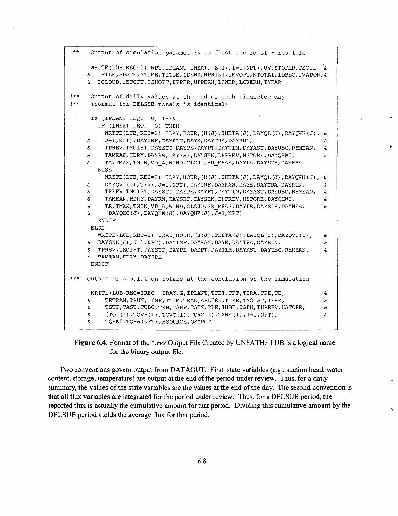
!** Output of simulation parameters to first record of *.res file

WRITE(LUB,REC=1) NPT,IPLANT,IHEAT,(Z(I),1=1,NPT),UV,STOPHR,TSOIL, S& IFILE,SDATE,STIME,TITLE,IDEND,NPRINT,IEVOPT,NTOTAL,IDBEG, IVAPOR,&& ICLOUD,IETOPT,ISHOPT,UPPER,UPPERH,LOWER,LOWERH,IYEAR

!** Output of daily values at the end of each simulated day!** (format for DELSUB totals is identical)

IF (IPLANT .EQ. 0) THENIF (IHEAT .EQ. 0) THENWRITE(LUB,REC=2) IDAY,HOUR,(H(J),THETA(J),DAYQL(J),DAYQVH(J), &

& J=l,NPT) , DAYINF,DAYRAN,DAYE,DAYTRA, DAYRUN, && TPREV, TMOIST, DAYSTP, DAYPE, DAYPT, DAYTIM, DAYAST, DAYUBC, RHMEAN, && TAMEAN, HDRY,DAYRN,DAYSHF,DAYSEN,DHPREV,HSTORE,DAYQHWO, && TA, TMAX, TMIN,VD_A,WIND,CLOUD,SR_MEAS,DAYLE,DAYSDH,DAYHBE

ELSE

WRITE(LUB,REC=2) IDAY,HOUR,(H(J),THETA(J),DAYQL(J),DAYQVH(J), && DAYQVT(J) , T(J),J=l,NPT),DAYINF,DAYRAN,DAYE,DAYTRA,DAYRUN, && TPREV,TMOIST,DAYSTP,DAYPE,DAYPT,DAYTIM,DAYAST,DAYUBC, RHMEAN, && TAMEAN,HDRY, DAYRN,DAYSHF,DAYSEN,DHPREV,HSTORE,DAYQHWO, S& TA,TMAX, TMIN,VD_A,WIND,CLOUD,SR_MEAS,DAYLE,DAYSDH,DAYHBE, S& (DAYQHC(J),DAYQHW(J),DAYQHV(J),J=l, NPT)

ENDIFELSE

WRITE(LUB,REC=2) IDAY,HOUR, (H(J),THETA(J),DAYQL(J),DAYQVH(J), &5 DAYSNK(J),J=1,NPT),DAYINF,DAYRAN,DAYE,DAYTRA,DAYRUN, &6 TPREV, TMOIST, DAYSTP,DAYPE,DAYPT,DAYTIM,DAYAST,DAYUBC,RHMEAN, && TAMEAN,HDRY,DAY S DHENDIF

!** Output of simulation totals at the conclusion of the simulation

WRITE(LUB,REC=IREC) IDAY,G,IPLANT,TPET, TPT, TTRA, TPE, TE, && TETRAN,TRUN,TINF,TTIM,TRAN,APLIED,TIRR,TMOIST,TERR, S5 TSTP,TAST,TUBC,TRN,TSHF,TSEN,TLE,THBE,TSDH,THPREV,HSTORE, &6 (TQL(I),TQVH(I),TQVT(I),TQHC(I),TSNK(I),1=1,NPT), S& .TQHWO,TQHW(NPT),HSOURCE,OSMPOT

Figure 6.4. Format of the *.res Output File Created by IJNSATH. LUB is a logical namefor the binary output file.

Two conventions govern output from DATAOUT. First, state variables (e.g., suction head, watercontent, storage, temperature) are output at the end of the period under review. Thus, for a dailysummary, the values of the state variables are the values at the end of the day. The second convention isthat all flux variables are integrated for the period under review. Thus, for a DELSUB period, thereported flux is actually the cumulative amount for that period. Dividing this cumulative amount by theDELSUB period yields the average flux for that period.

6.8

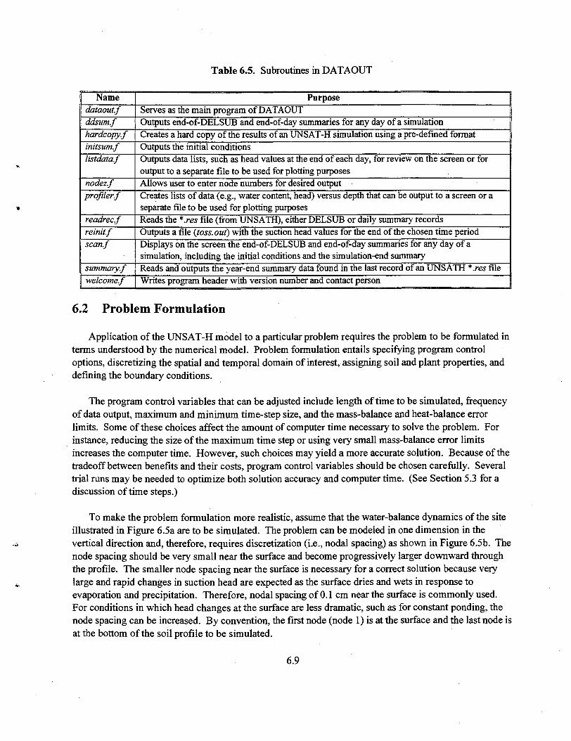
Table 6.5. Subroutines in DATAOUT

Namedataout.fddsum.fhardcopy.finitsum.flistdata./

nodez.fprofiler./

readrec.freinit.fscan./

summary./welcome./

PurposeServes as the main program of DATAOUTOutputs end-of-DELSUB and end-of-day summaries for any day of a simulationCreates a hard copy of the results of an UNSAT-H simulation using a pre-defined formatOutputs the initial conditionsOutputs data lists, such as head values at the end of each day, for review on the screen or foroutput to a separate file to be used for plotting purposesAllows user to enter node numbers for desired outputCreates lists of data (e.g., water content, head) versus depth that can be output to a screen or aseparate file to be used for plotting purposesReads the *.res file (from UNSATH), either DELSUB or daily summary recordsOutputs a file (toss, out) with the suction head values for the end of the chosen time periodDisplays on the screen the end-of-DELSUB and end-of-day summaries for any day of asimulation, including the initial conditions and the simulation-end summaryReads and outputs the year-end summary data found in the last record of an UNSATH *.res fileWrites program header with version number and contact person

6.2 Problem Formulation

Application of the UNSAT-H model to a particular problem requires the problem to be formulated interms understood by the numerical model. Problem formulation entails specifying program controloptions, discretizing the spatial and temporal domain of interest, assigning soil and plant properties, anddefining the boundary conditions.

The program control variables that can be adjusted include length of time to be simulated, frequencyof data output, maximum and minimum time-step size, and the mass-balance and heat-balance errorlimits. Some of these choices affect the amount of computer time necessary to solve the problem. Forinstance, reducing the size of the maximum time step or using very small mass-balance error limitsincreases the computer time. However, such choices may yield a more accurate solution. Because of thetradeoff between benefits and their costs, program control variables should be chosen carefully. Severaltrial runs may be needed to optimize both solution accuracy and computer time. (See Section 5.3 for adiscussion of time steps.)

To make the problem formulation more realistic, assume that the water-balance dynamics of the siteillustrated in Figure 6.5a are to be simulated. The problem can be modeled in one dimension in thevertical direction and, therefore, requires discretization (i.e., nodal spacing) as shown in Figure 6.5b. Thenode spacing should be very small near the surface and become progressively larger downward throughthe profile. The smaller node spacing near the surface is necessary for a correct solution because verylarge and rapid changes in suction head are expected as the surface dries and wets in response toevaporation and precipitation. Therefore, nodal spacing of 0.1 cm near the surface is commonly used.For conditions in which head changes at the surface are less dramatic, such as for constant ponding, thenode spacing can be increased. By convention, the first node (node 1) is at the surface and the last node isat the bottom of the soil profile to be simulated.

6.9

Precipitation

I tEvaporation

Hourly Rainfall

IET

t= f(PET)

' Includes Plants,* Vapor Flow

Nodes

Unit GradientDrainage

(a)1(b)

Figure 6.5. Example Problem Formulation: a) Site Description, b) Model Representation

Other things being equal, a larger number of nodes provides a more accurate solution, but requiresmore computer time. Uncertainties regarding the sufficiency of the number of nodes for a particularproblem may require repetition of the simulation with more nodes to check the prior solution. If thesolution remains essentially the same, additional nodes are not necessary. If the solution changessignificantly, then the original number of nodes may have been insufficient (i.e., the node spacing was toolarge). In that case, repetition of the simulation with smaller node spacing is needed until the solutiondoes not change appreciably.

6.10

In the example shown in Figure 6.5a, the soil type changes at the midpoint of the profile. This kind ofchange may make the solution difficult if the hydraulic properties of the two soils are significantlydifferent. Therefore, the node spacing near the interface of two soils should be decreased (i.e., morenodes in that vicinity), until the solution does not change.

After discretizing the spatial domain, the next step is to assign soil properties. In the example ofFigure 6.5a, there are two soil types. Nodes within each soil are assigned the properties of that soil. Inother instances, soil layering may be less clearly defined. In those cases, the dominant soil types areidentified and soil properties assigned accordingly.

Once soil properties have been assigned, initial conditions must be specified. This step isaccomplished for all simulations by specifying the head values at the start of the simulation period. Ifheat flow is being modeled, the temperature values must also be specified. In most instances, soilcharacterization data consists of neutron probe measurements of water content at several depths within theprofile. Based on these measurements, water contents must be assigned to each node. Unfortunately, themeasurement depths are unlikely to coincide with the nodal depths. Therefore, values must be inter-polated. The nodal water contents must then be converted to head values (the, initial conditions requiredby UNSAT-H) according to the soil hydraulic properties assigned to the respective node.

The next stage in problem formulation is to describe the plant community, if one is present. Requiredplant data include fraction of surface covered by plants, dates of germination and death, rooting depths,and responses to moisture-related stress.

The lower and upper boundary conditions must be identified next. In Figure 6.5b, the lower boundaryis known to be permeable, but measurements of the drainage rate are not available, and the head at thelowest node is not likely to remain constant for long periods of time. As an approximation, a unitgradient can be assumed to exist at the lower boundary because the boundary is well below the root zone.In the absence of heat flow measurements, a rough estimate of the geothermal gradient can be used.

For the surface boundary, daily weather data must be provided if heat flow and evaporation are beingmodeled. Daily weather data must also be provided if evaporation is being modeled using the PETconcept and the code is to calculate the daily PET. Otherwise, daily PET must be provided. These valuesare calculated external to the UNSAT-H code using programs such as FAOPET (Doorenbos and Pruitt1977). Precipitation rates can be entered directly.

When a problem is to be solved using UNSAT-H, the necessary data must be collected into a *.inpfile in the format required by the preprocessor program, DATAINH. That format is specified inAppendix A.

6.11

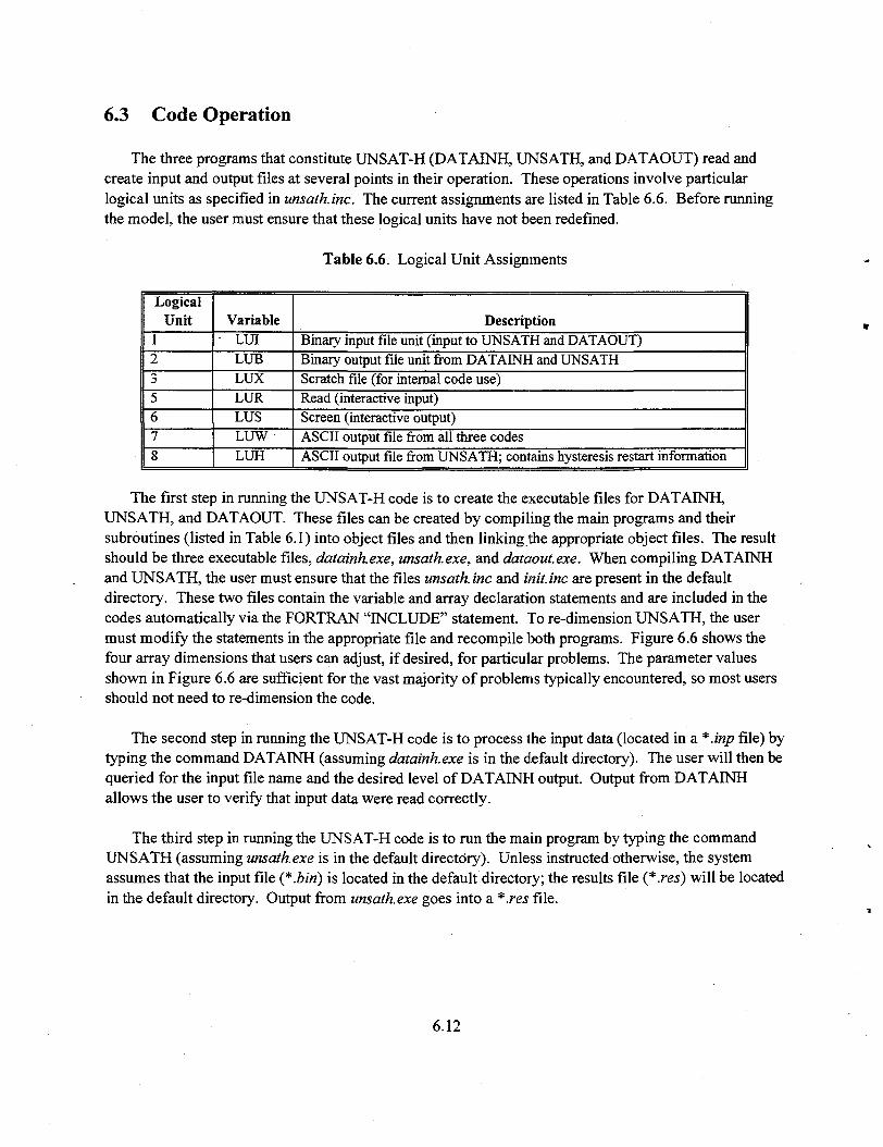
6.3 Code Operation

The three programs that constitute UNSAT-H (DATATNH, UNSATH, and DATAOUT) read andcreate input and output files at several points in their operation. These operations involve particularlogical units as specified in unsathinc. The current assignments are listed in Table 6.6. Before runningthe model, the user must ensure that these logical units have not been redefined.

Table 6.6. Logical Unit Assignments

LogicalUnit

1235678

VariableLUILUBLUXLURLUSLUWLUH

DescriptionBinary input file unit (input to UNSATH and DATAOUT)Binary output file unit from DATAINH and UNSATHScratch file (for internal code use)Read (interactive input)Screen (interactive output)ASCII output file from all three codesASCII output file from UNSATH; contains hysteresis restart information

The first step in running the UNSAT-H code is to create the executable files for DATAINH,UNSATH, and DATAOUT. These files can be created by compiling the main programs and theirsubroutines (listed in Table 6.1) into object files and then linking the appropriate object files. The resultshould be three executable files, datainhexe, unsathexe, and dataout.exe. When compiling DATAINHand UNSATH, the user must ensure that the files unsathAnc and init.inc are present in the defaultdirectory. These two files contain the variable and array declaration statements and are included in thecodes automatically via the FORTRAN "INCLUDE" statement. To re-dimension UNSATH, the usermust modify the statements in the appropriate file and recompile both programs. Figure 6.6 shows thefour array dimensions that users can adjust, if desired, for particular problems. The parameter valuesshown in Figure 6.6 are sufficient for the vast majority of problems typically encountered, so most usersshould not need to re-dimension the code.

The second step in running the UNSAT-H code is to process the input data (located in a *.inp file) bytyping the command DATAINH (assuming datainhexe is in the default directory). The user will then bequeried for the input file name and the desired level of DATAINH output. Output from DATAINHallows the user to verify that input data were read correctly.

The third step in running the UNSAT-H code is to run the main program by typing the commandUNSATH (assuming unsathexe is in the default directory). Unless instructed otherwise, the systemassumes that the input file (*.bin) is located in the default directoiy; the results file (*.res) will be locatedin the default directory. Output from unsa.th.exe goes into a *.res file.

6.12

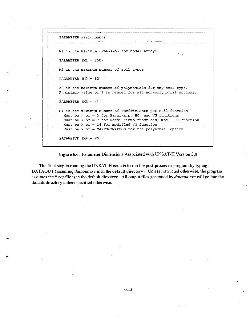
PARAMETER assignments

Ml is the maximum dimension for nodal arrays

PARAMETER (Ml = 250)

M2 is the maximum number of soil types

PARAMETER (M2 = 10)

M3 is the maximum number of polynomials for any soil type.

A minimum value of 1 is needed for all non-polynomial options.

PARAMETER (M3 = 4)

M4 is the maximum number of coefficients per soil functionMust be > or = 5 for Haverkamp, BC, and VG functionsMust be > or = 7 for Rossi-Nimmo functions, mod. .BC functionMust be > or = 14 for modified VG functionMust be > or = MAXPOL*MAXCOE for the polynomial option

PARAMETER (M4 = 20)

Figure 6.6. Parameter Dimensions Associated with UNSAT-H Version 3.0

The final step in running the UNSAT-H code is to ran the post-processor program by typingDATAOUT (assuming dataout.exe is in the default directory). Unless instructed otherwise, the programassumes the *.res file is in the default directory. All output files generated by dataoutexe will go into thedefault directory unless specified otherwise.

6.13

7.0 Example Simulations

Eight examples are provided in this section to illustrate how various UNSAT-H options work. Thefirst four examples are verification tests of infiltration, drainage, heat flow, and hysteresis portions of theUNSAT-H code. The remaining four examples are simulations of water flow in a layered soil system,water and heat flow in a layered system, plant transpiration, and a multiyear simulation. Included in theinfiltration verification test is a demonstration of the new solution option (the modified Picard method).Included in the heat flow verification test is a demonstration of the new solution control option involvingthe heat balance error.

7.1 Verification of Infiltration

Haverkamp et al. (1977) performed several infiltration simulations using different models based onthe nonlinear flow equation. One of those models, the head-based implicit model (No. 4 in theHaverkamp paper) is the same as that used in UNSAT-H. To simultaneously verify the infiltrationcomponent of UNSAT-H and provide an example of how UNSAT-H works, the Haverkamp et al. (1977)infiltration problem was simulated with UNSAT-H. The UNSAT-H results are compared with those ofHaverkamp et al. (1977) and with an approximate analytic solution derived by Philip (1969). Thisverification test was also conducted by Fayer and Jones (1990). Additional simulations were conductedto demonstrate the use of a new solution feature called the modified Picard method.

7.1.1 Problem Description

Haverkamp et al. (1977) used two soil types: a clay (Yolo light clay) and a sand. Table 7.1 shows thesoil hydraulic property coefficients used. The soil profile depths were 250 and 90 cm for the clay and

Table 7.1. Parameters Used in the Infiltration Simulations

Parameter

6X (cm3 cm"3)

0r (cm3 cm"3)

or (cm"1)

/?(unitless)

. he (cm)

Ks (cm hr"1)

A (cm"1)

B (unitless)

he (cm), for the conductivity function

Clay

0.495

0.124

739.0

4.0

1.0

4.428 xlO"2

124.6

1.77

0.0

Sand

0.287

0.075

1.611 xlO6

3.96

1.0

34.0

1.175 xlO6

4.74

1.0

7.1

sand, respectively. Depth increments were 1.0 cm. For the lower boundary, the head at the bottom nodewas held constant at the initial value of 600 cm for the clay and 61.4 cm for the sand. For the upperboundary, the head at the surface node was held constant at 0.0 cm for the clay and at 20.73 cm for thesand. The minimum and maximum time steps were 0.0125 and 0.15 hr, respectively, for the clay, and10"5 and 0.0025 hr, respectively, for the sand. Haverkamp et al. (1977) allowed the time step to varybetween 40 and 500 s (0.0111 to 0.139 hr) for the clay and used a constant time step of 5 s(1.39x 10"3 hr)for the sand. Figures B.I (clay) and B.2 (sand) of Appendix B show the input files.

7.1.2 Results

Figure 7.1 illustrates the results from Haverkamp et al. (1977, Figure 6), the quasi-analytic seriessolution (Philip 1969), and UNSAT-H. According to Haverkamp et al. (1977), the series solution is valid(Le., the solution converges) only for times less than 600 hr for the clay and 0.29 hr for the sand. For bothsoils, the agreement among the results of Haverkamp et al. (1977), Philip (1969), and UNSAT-H isexcellent. This agreement indicates that the infiltration component of UNSAT-H performs satisfactorilyfor this type of problem. Figures B.3 and B.4 of Appendix B show the clay and sand output files.

The clay and sand tests were repeated using the new modified Picard solution technique (Celia et al.1990). The test names were clayst, and sandst. The maximum number of iterations was increased tofive to enable the modified Picard method to function. For comparison purposes, clay and sand werererun using the same maximum number of iterations. Table 7.2 shows that the new solution techniquedramatically lowered the mass balance error.

7.2 Verification of Drainage

Kool et al. (1985) used the parameter estimation program ONESTEP to fit drainage data from anoutflow experiment. The program estimated values for three parameters of the van Genuchten waterretention function. The Kool et al. (1985) experiment was simulated with UNSAT-H, using their fittedparameters, to verify the drainage component of UNSAT-H and the implementation of the van Genuchtenwater retention and Mualem hydraulic conductivity models. This verification test was also conducted byFayer and Jones (1990).

7.2.1 Problem Description

Kool et al. (1985) sampled an undisturbed core of silty loam soil from a field in Virginia. Theyequilibrated the core at zero suction head in a Tempe pressure cell with a ceramic plate located at thebottom. The soil core was 3.95 cm long and 5.4 cm in diameter. The porous ceramic plate was 0.57 cmthick. After a complete cycle of drying and wetting, the core was subjected to an air pressure of 1000 cm.The drainage that resulted was monitored until it nearly ceased.

7.2

0.10

1 0.08

eico

£ 0.06 -

0.04

A A

A Philip Infil

UNSATH Infil

Haverkamp Infil

Philip Cum Infil

UNSATH Cum Infil

- - Haverkamp Cum Infil

300 600

Time (hr)

900

60

40

20 -f|

J-0

1200

36

Philip Infil

UNSATH InfilHaverkamp Infil

A Philip Cum Infil

UNSATH Cum Infil

Haverkamp Cum Infil

0.0 0.2 0.4

Time (hr)

0.6 0.8

Figure 7.1. Infiltration Rate and Cumulative Infiltration Versus Time as Determined Using the Philip(1969) Solution, the Numerical Code of Haverkamp et al. (1977), and UNSAT-H

7.3

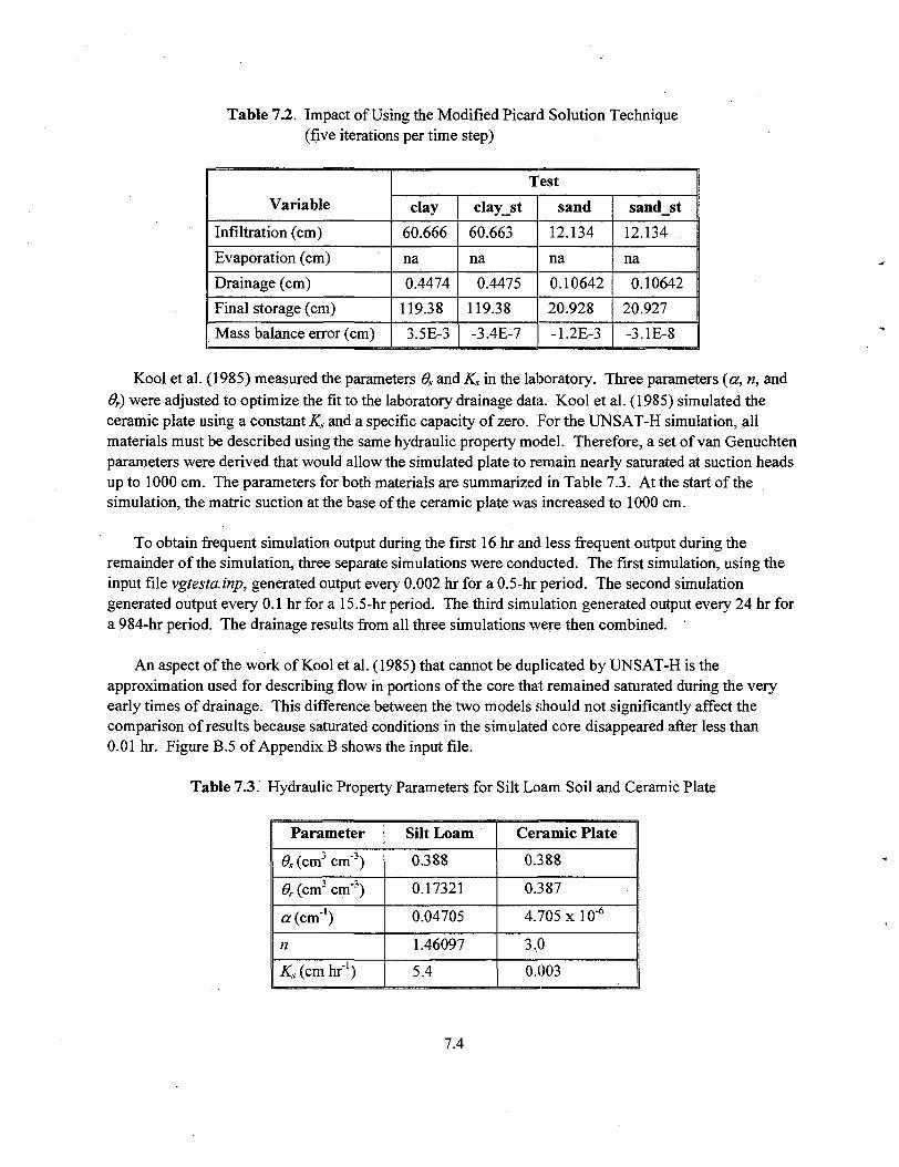
Table 7.2. Impact of Using the Modified Picard Solution Technique(five iterations per time step)

Variable

Infiltration (cm)

Evaporation (cm)

Drainage (cm)

Final storage (cm)

Mass balance error (cm)

Test

clay

60.666

na

0.4474

119.38

3.5E-3

clay_st

60.663

na

0.4475

119.38

-3.4E-7

sand

12.134

na

0.10642

20.928

-1.2E-3

sand_st

12.134

na

0.10642

20.927

-3.1E-8

Kool et al. (1985) measured the parameters 6S and Ks in the laboratory. Three parameters (a, n, and0r) were adjusted to optimize the fit to the laboratory drainage data. Kool et al. (1985) simulated theceramic plate using a constant Ks and a specific capacity of zero. For the UNSAT-H simulation, allmaterials must be described using the same hydraulic property model. Therefore, a set of van Genuchtenparameters were derived that would allow the simulated plate to remain nearly saturated at suction headsup to 1000 cm. The parameters for both materials are summarized in Table 7.3. At the start of thesimulation, the matric suction at the base of the ceramic plate was increased to 1000 cm.

To obtain frequent simulation output during the first 16 hr and less frequent output during theremainder of the simulation, three separate simulations were conducted. The first simulation, using theinput file vgtesta.inp, generated output every 0.002 hr for a 0.5-hr period. The second simulationgenerated output every 0.1 hr for a 15.5-hr period. The third simulation generated output every 24 hr fora 984-hr period. The drainage results from all three simulations were then combined.

An aspect of the work of Kool et al. (1985) that cannot be duplicated by UNSAT-H is theapproximation used for describing flow in portions of the core that remained saturated during the veryearly times of drainage. This difference between the two models should not significantly affect thecomparison of results because saturated conditions in the simulated core disappeared after less than0.01 hr. Figure B.5 of Appendix B shows the input file.

Table 7.3. Hydraulic Property Parameters for Silt Loam Soil and Ceramic Plate

Parameter

6S (cm3 cm'3)

6r (cm3 cm'3)

a (cm'1)

n

Kx (cm hr"1)

Silt Loam

0.388

0.17321

0.04705

1.46097

5.4

Ceramic Plate

0.388

0.387

4.705 xlO'6

3,0

0.003

7.4

7.2.2 Results

Figure 7.2 shows the cumulative drainage results from the UNSAT-H simulations, along with thesimulation results and laboratory measurements from Kool et al. (1985). The close agreement among thetwo code solutions and the measurements indicates that UNSAT-H simulates drainage correctly. Theagreement also indicates that the van Genuchten retention function and the Mualem conductivity modelhave been implemented correctly in UNSAT-H. Figure B.6 of Appendix B shows the output file.

18

a Measured

• ONESTEP

— UNSATH

0.01 0.10 1.00 10.00

Time (hr)

100.00 1000.00

Figure 7.2. Cumulative Drainage Versus Time as Determined by Kool et al. (1985) and UNSAT-H

7.3 Verification of Heat Flow

In this test, the UNSAT-H model is used to simulate the diurnal variation in soil temperatures causedby an imposed cyclic variation in soil surface temperature. This verification test was also conducted byFayer and Jones (1990).

Campbell (1977) reported an analytic solution to a heat conduction problem in which the temperature(7) at the soil surface varies by

(7.1)

where T = mean soil surface temperature, K= amplitude of soil surface temperature, K

co = angular frequency of the soil surface temperature oscillation, hr"1

t = time, hr.

7.5

Assuming the soil is uniform and infinitely deep, the solution for a temperature wave is (Campbell 1977):

T(z,t) = f + A(Q)e~zlz<> sin[o)(t-6)-z/zd] (7.2)

where

co = 2n/24 (7.3)

and

(7.4)

where zj is the damping depth, which is the depth at which the temperature fluctuation has been reducedto 37% (i.e., 1/e) of its surface value. For this case, the angular frequency yields a complete surfacetemperature cycle in 24 hr. To specify that the peak temperature occurs at noon, as is done for thisexample, the t value in Equation (7.2) is modified by subtracting 6 hr.

7.3.1 Problem Description

A 1-m-deep soil profile is subjected to a temperature variation of 10K from a mean surface tempera-ture of 288K occurring at noon. A total of 101 nodes, evenly spaced 1 cm apart, are used to discretize thesoil profile. The soil type is a loamy sand known as lysimeter sand or L-soil (Rockhold et al. 1988). Thehydraulic properties are described using the Brooks-Corey functions, with 6S = 0.4326, #. = 0.0381,he = 9.4 cm, b = 1.2846, and Ks = 35.3 cm/hr. The thermal properties are taken from Cass et al. (1981) forlysimeter sand at 22.5°C. The initial temperature at all nodes is 288K; the initial suction at all nodes is100 cm ($ = 0.1007).

A horizontal profile is simulated to minimize water movement. Vapor flow is not included so thatwater contents and thermal conductivities remain constant during the simulation. Figure B.7 ofAppendix B shows the input file. For the analytic solution, kh = 27.448 J cm"1 mole'1 K"1,Ch = 1.1927 J cm"3 K"1, andz</= 13.26 cm.

7.3.2 Results

Figure 7.3 shows the soil temperature results for the analytic solution and UNSAT-H. The closenessof the match between the analytic solution and the simulated temperatures at all depths and timesindicates that UNSAT-H correctly solves the heat conduction equation. Figure B.8 of Appendix B showsthe output file.

7.6

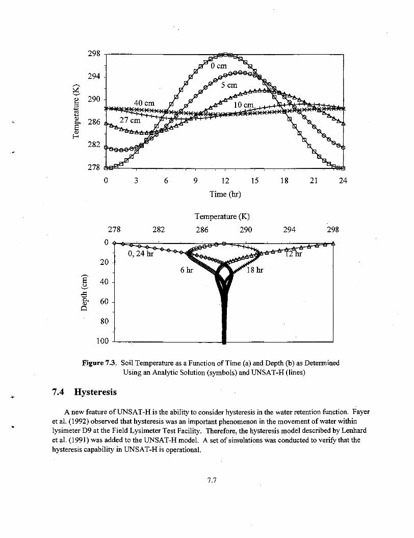
278 A0 9 12 15

Time (hr)

18 21 24

o

278 282

Temperature (K)

286 290 294 298

u <

20 -

40 -

60 -

80 -

100 -

^ 2 4 h T ~ ^ ~ ^ - ^ ^ ^

6 h r ^ ^ ^V^18hr

V

11Figure 7.3. Soil Temperature as a Function of Time (a) and Depth (b) as Determined

Using an Analytic Solution (symbols) and UNSAT-H (lines)

7.4 Hysteresis

A new feature of UNSAT-H is the ability to consider hysteresis in the water retention function. Fayeret al. (1992) observed that hysteresis was an important phenomenon in the movement of water withinlysimeter D9 at the Field Lysimeter Test Facility. Therefore, the hysteresis model described by Lenhardet al. (1991) was added to the UNSAT-H model. A set of simulations was conducted to verify that thehysteresis capability in UNSAT-H is operational.

7.7

7.4.1 Problem Description

Lenhard et al. (1991) conducted an experiment in which a sand-filled column was subjected to afluctuating water table while water contents and matric potentials were monitored throughout the column.The water table position was changed four times: lowered, then raised, then lowered, then raised back tothe original elevation. A single-beam gamma system was used to measure water saturation at multiplelevels within the column during these changes. The values at the 70-cm elevation above the base of thecolumn were used for the UNSAT-H verification test. Lenhard et al. (1991) also simulated the experi-ment with a computer code that incorporated their hysteresis model. Their measured and simulatedvalues of water saturation are reported in Fayer (1993).

The hydraulic properties are described using the van Genuchten water retention function, withds = 0.355, dr = 0.06035, a = 0.042 cm"1, n = 5.25, and Ks = 119 cm/hr. The Mualem conductivity modelwas used with a pore interaction exponent value of 0.5. Only two additional parameters were needed: themaximum amount of entrapped air (Snr) and the imbibition ar, parameter for the van Genuchten retentionfunction. As done by Lenhard et al. (1991), the parameter 'Snr was set to 0.25 and the parameter a, wasset equal to la^, the comparable parameter for drainage. The final specification was that up to sevenhysteretic paths could be used by the hysteresis model. Figure B.9 of Appendix B shows a portion of theinput file used for this simulation.

Three separate simulations were conducted: 1) no hysteresis or air entrapment, 2) no hysteresis butair entrapment, and 3) hysteresis and air entrapment.

7.4.2 Results

Figure 7.4 shows that the UNSAT-H results are nearly identical to the Lenhard simulation results forall three cases. Figure 7.4 also shows that the best match to the measured saturation values was achievedusing the full model of hysteresis with air entrapment. The hysteresis option was judged to beoperational. Figure B. 10 of Appendix B shows the output file.

7.5 Layered Soil Simulation

The UNSAT-H model is used to simulate the water balance of various protective barrier designs. Inthis example, the functioning of a specific barrier design was simulated for weather conditions in 1962.This verification test was also conducted by Fayer and Jones (1990).

7.5.1 Problem Description

The protective barrier concept limits deep percolation by relying on the capillary break created whenfine-textured soils are placed over coarse-textured soils. In one of the barrier designs, the top 30 cm ofmaterial is composed of the Composite soil described by Fayer et al. (1985) and gravel 0.5 to 1.0 cm indiameter (15% by weight). The material between the 30- and 150-cm depths is Composite soil. Gravel

7.8

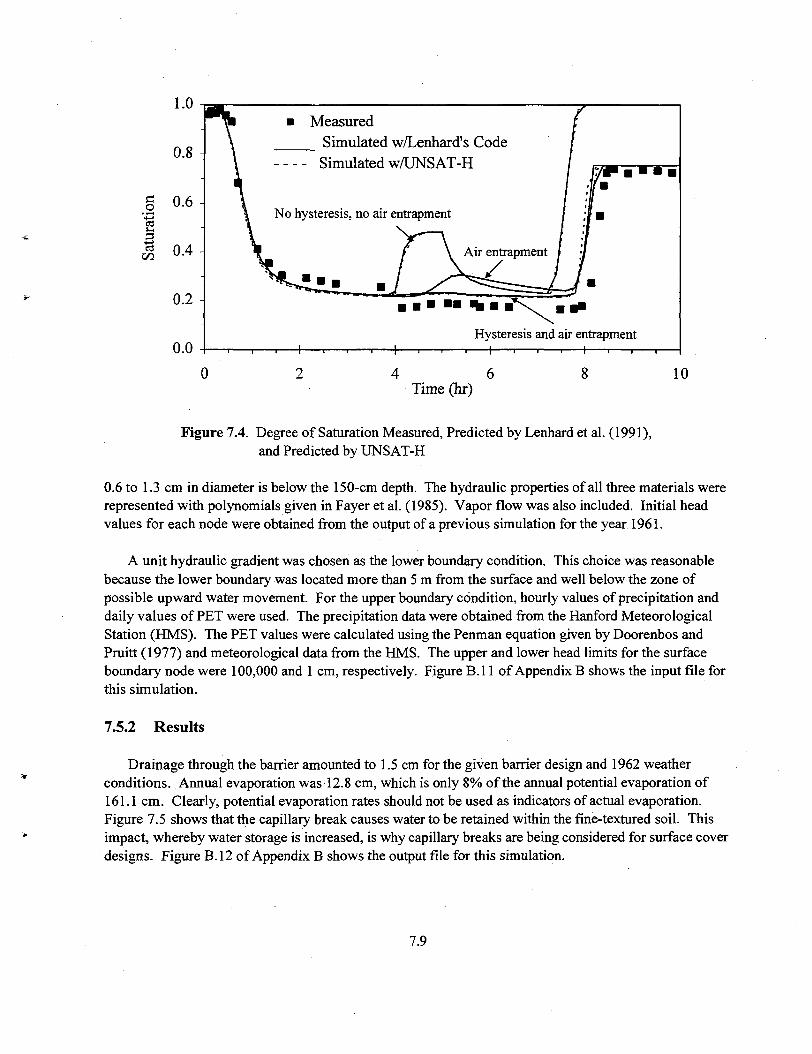
g 0.6-1

1I 0.4 -]

MeasuredSimulated w/Lenhard's CodeSimulated w/UNSAT-H

No hysteresis, no air entrapment

Hysteresis and air entrapment

4 6Time (hr)

10

Figure 7.4. Degree of Saturation Measured, Predicted by Lenhard et al. (1991),and Predicted by UNSAT-H

0.6 to 1.3 cm in diameter is below the 150-cm depth. The hydraulic properties of all three materials wererepresented with polynomials given in Fayer et al. (1985). Vapor flow was also included. Initial headvalues for each node were obtained from the output of a previous simulation for the year 1961.

A unit hydraulic gradient was chosen as the lower boundary condition. This choice was reasonablebecause the lower boundary was located more than 5 m from the surface and well below the zone ofpossible upward water movement. For the upper boundary condition, hourly values of precipitation anddaily values of PET were used. The precipitation data were obtained from the Hanford MeteorologicalStation (HMS). The PET values were calculated using the Penman equation given by Doorenbos andPruitt (1977) and meteorological data from the HMS. The upper and lower head limits for the surfaceboundary node were 100,000 and 1 cm, respectively. Figure B.I 1 of Appendix B shows the input file forthis simulation.

7.5.2 Results

Drainage through the barrier amounted to 1.5 cm for the given barrier design and 1962 weatherconditions. Annual evaporation was 12.8 cm, which is only 8% of the annual potential evaporation of161.1 cm. Clearly, potential evaporation rates should not be used as indicators of actual evaporation.Figure 7.5 shows that the capillary break causes water to be retained within the fine-textured soil. Thisimpact, whereby water storage is increased, is why capillary breaks are being considered for surface coverdesigns. Figure B.12 of Appendix B shows the output file for this simulation.

7.9

Water Content (cm /cm )

Figure 7.5. Water Content Profiles Within a Layered Soil

7.6 Layered Soil Simulation with Heat Flow

The layered soil simulation in Section 7.5 was repeated with the heat flow option to demonstrate theconcurrent flow of water and heat. This verification test was also, conducted by Fayer and Jones (1990).

7.6.1 Problem Description

The input file used in Section 7.5 was modified for this example to include the addition of soilthermal properties, aerodynamic coefficients, time-stepping controls, initial suction heads andtemperatures for the end of day 143, and weather data.

Because hourly output was desired, the simulation was conducted for only three days: 144, 145, and146. Precipitation on day 144 amounted to 1.30 cm; no precipitation occurred on days 145 and 146.

Thermal conductivity parameters for the barrier materials were taken from Cass et al. (1984). For theComposite soil and the Composite-gravel mix, the parameters for the Portneuf silt loam at 32.5°C wereused. For the gravel layer, the parameters for the Lysimeter sand at 22.5°C were used. Althoughprovided by Cass et al. (1984), parameters for the enhancement factor (77) were chosen to provide 77values of 1 (i.e., no enhancement).

The measurement heights for temperature and wind speed were 0.914 and 15.24 m, respectively.Data from Ligotke (1988) indicate a roughness length for momentum of 4.9 x 10"4 m for a soil mixcontaining 70% silt loam and 30% 0.7-cm-diameter gravel. The roughness length for heat was assumedto equal that for momentum.

7.10

The minimum and maximum time-step sizes were reduced from 10~7 and 1.0 to 10"8 and 0.025 hr,respectively. The mass balance criterion was decreased from 10"4 to 10"5 cm. In addition, changes inhead per time step were limited to 2 x 104 cm; otherwise, the time-step size was reduced by half. Theiteration number for water flow was increased from 2 to 3. The iteration number for heat flow was 2.Hourly rather than daily output was specified.

Initial suction head values for the end of day 143 were obtained from the results of the simulation inSection 7.4. The lower suction head limit for the surface boundary node was 1 cm; no upper limit wasspecified. Initial soil temperature values for the end of day 143 were specified using the historicalaverage for May for the 91.4-cm depth (Hoitink et al. 1999). That average, 15.9°C, was applied to allnodes. Figure B.13 of Appendix B shows the input file for this simulation.

7.6.2 Results

Figure 7.6 shows the surface energy fluxes, suction heads of the top two nodes, air and surface. temperatures, and precipitation for the 3-day period. In Figure 7.6a, the latent heat flux is small on day144 because of the precipitation. The abrupt changes in soil heat flux on this day are caused by theintermittent nature of the precipitation (see Figure 7.6d). On day 145, the latent heat flux rises steadilyduring the day until 1400 hr. By that time, the surface node has dried to a suction head of 6.2 x 105 cm(Figure 7.6b). This surface dryness reduces the latent heat flux (i.e., the evaporation rate). On day 146,the surface node again dries to a high suction head (1.2 x 106) by midday. As on day 145, the dryness ofthe surface limits the latent heat flux during midday.

The results in Figure 7.6c show that the surface temperature remains higher than air temperaturethroughout the 3-day period. For the rainy day 144 and the nighttime of days 145 and 146, the surfacetemperature is within 5K of air temperature. During the daytime of days 145 and 146, however, thesurface temperature exceeds the air temperature by as much as 18K. Peak surface temperature occursbetween the noon peak of net radiation and the 1500 hr peak of air temperature.

Total evaporation for this 3-day period was 0.557 cm, compared to 0.386 cm for the same period forthe simulation in Section 7.5. Because of the time-step differences between the two simulations, theisothermal problem in Section 7.5 was repeated with time-step information identical to the problemdescribed in this section. The results from this third simulation show total evaporation to be 0.375 cm.

This simulation of a layered soil with concurrent water and heat flow was repeated using the option ofcontrolling the time step according to the heat balance error. The control was 0.001 J/m2. Using theenergy balance control of the time step caused a doubling of the number of time steps (to 4838). Theimpact from using this criterion was very minor for the water balance variables. Both evaporation anddrainage changed by less than 0.01%. The impact was a bit more substantial for the mass balance error,which dropped 10-fold to -2 x 10"5 cm. As expected, the impact on the heat balance error was substantial.The heat balance error dropped 4-fold to 0.4 J/m2, allowing the energy balance check to be judgedoperational. Figure B.14 of Appendix B shows the output file for this simulation.

7.11

600

300 -

3

E

I

Energy Fluxes

Net RadiationSensible HeatLatent Heat

' Surface Heat

l.E+08

4.E+06;

£ l.E+04co

l.E+02 i

1.E+00

320

Suction Heads ( b )

1«300

8.I 290 -

280

0.20

0.15 -

•2 0.10 -

0.05 -J

Temperatures

i Air :| Surface;

• ' • • - - • • ' 'i-—-—~^Z:--

- - . ( C )

0.00

143 144 145Day of Year 1962

146

Figure 7.6. Simulation Results for Water and Heat Flow in a Layered Soil: a) energy fluxes at thesoil surface, b) suction heads at and 0.1 cm below the soil surface, c) air and soilsurface temperature, and d) precipitation

7.12

7.7 Transpiration Simulation

This simulation was conducted to demonstrate how UNSAT-H might be used to model transpiration.This simulation was also conducted by Fayer and Jones (1990).

7.7.1 Problem Description

Two 15.2-m-deep lysimeters were constructed in the 200 Area at the Hanford Site to study downwardwater movement (Hsieh et al. 1973; Brownell et al. 1975). One of the two lysimeters had a closedbottom. Year after year, soil water contents measured in the closed-bottom lysimeter appeared to indicateno downward water movement (e.g., Jones 1978). This observation was always attributed to evaporation;the plant component was always neglected. Through photographs, Gee and Heller (1985) documentedthat Russian thistle plants were growing on the lysimeter during 1974. Unfortunately, the plantcommunity was never quantitatively characterized. Therefore, a simulation was conducted to predict thewater dynamics in the lysimeter in 1974.

The lysimeter, which is 1829 cm (60 ft) deep, was represented with 43 nodes. Figure 7.7 shows theparameters used for the Brooks-Corey hydraulic functions. These parameters were taken from Fayer andJones (1990). Initial conditions (i.e., initial head values) were obtained from the *.res file of a simulationfor the year 1973.

The plant data needed for the simulation include the Iu, fraction of the soil surface that is bare,rooting density and depth, and plant response to water content (the sink functions). In lieu of sitemeasurements, the plant parameters had to be estimated. The assumed ILA and maximum rooting depthare shown in Figure 7.8. Note that growth started on day 121 and stopped on day 274 of the simulation.In addition, roots were allowed to penetrate to the 3-m depth by day 244. The bare fraction of soil surfacewas 0.94. Rooting density was calculated using Equation (4.49) such that a = 4.0, b = 0.034, and c = 1.0.Finally, the sink function (Figure 4.5) was approximated with 6W = 0.031, 0j= 0.0374, and 9n = 0.4125.Figure B.15 of Appendix B shows the input file for this simulation.

7.7.2 Results

Although they covered only 6% of the lysimeter surface, the simulated plants were able to remove2.4 cm of water from the lysimeter. This transpired water represents 18% of the 13.5 cm of precipitation.Evaporation removed an additional 16 cm of water, resulting in a combined evapotranspiration loss of18.4 cm (versus 16.9 cm when plants are not present). Storage in the lysimeter decreased by 5.0 cmduring the year, a condition that is not conducive to long-term deep drainage or recharge. Figure B.I6 ofAppendix B shows the output file for this simulation.

7.13

Sand200 East Lysimeter0, = 0.4142

er = o.ohc = 29.8 cm6=1.63

0.0

10 100 1000

Suction Head (cm)

10000 100000

l.E+02 u

Sand200 East Lysimeter6>.= 0.41426r = 0.0he = 29.8 cm6=1.63K, =24.8cm/hr

10 100 1000

Suction Head (cm)

10000 100000

Figure 7.7. Soil Hydraulic Properties for the 200 Area Lysimeter

7.8 Multiyear Simulation

A new feature of UNSAT-H is the ability to conduct multiyear simulations. Fayer and Walters(1995) simulated 35 years of recharge in the soil type known locally as Ephrata sandy loam using anexternal batch program. This simulation was conducted without plants to understand possible rechargerates if this soil type was disturbed. To demonstrate the multiyear simulation capability, the Fayer andWalters (1995) simulation was repeated.

7.14

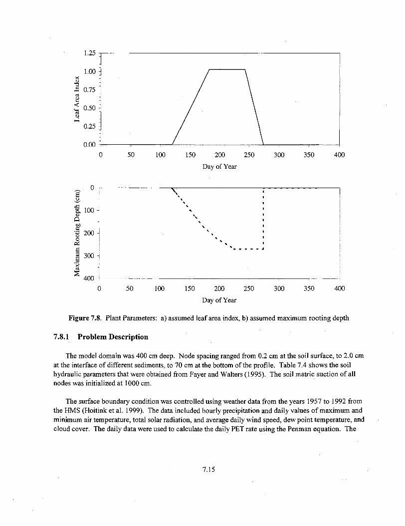
1.25

1.00 :

xa)

T3

£ 0.75CO

2£ 0.50 -.3 :

0.25 -

0.00 V0 50 100 150 200 250

Day of Year

300 350 400

£

& 1 0° 'Q

1 200 -o

Q£

| 300 -'xc a "•

400 -

\x

XX

s

s •

•

50 100 150 200 250

Day of Year

300 350 400

Figure 7.8. Plant Parameters: a) assumed leaf area index, b) assumed maximum rooting depth

7.8.1 Problem Description

The model domain was 400 cm deep. Node spacing ranged from 0.2 cm at the soil surface, to 2.0 cmat the interface of different sediments, to 70 cm at the bottom of the profile. Table 7.4 shows the soilhydraulic parameters that were obtained from Fayer and Walters (1995). The soil matric suction of allnodes was initialized at 1000 cm.

The surface boundary condition was controlled using weather data from the years 1957 to 1992 fromthe HMS (Hoitink et al. 1999). The data included hourly precipitation and daily values of maximum andminimum air temperature, total solar radiation, and average daily wind speed, dew point temperature, andcloud cover. The daily data were used to calculate the daily PET rate using the Penman equation. The

7.15

Table 7.4. Parameters Used in the Multiyear Simulation

Parameter

6S (cm3 cm'3)

Qr (cm3 cm"3)

a (cm"1)

n (unitless)

^-(cmhr"1)

Layer 1Sandy Loam

0 to 33 cm

0.47

0.0426

0.117

1.48

3.2

Layer 2Sandy Gravel33 to 71 cm

0.141

0.0128

0.117

1.48

0.592

Layer 3Sandy Gravel71 to 400 cm

0.0833

0.0084

0.0061

1.52

0.572

bottom boundary was considered deep enough to be unaffected by surface evaporation. Therefore, a unitgradient condition was specified for this boundary. Figure B.I 7 of Appendix B shows the input file forthis simulation.

7.8.2 Results

Figure 7.9 shows the predicted annual recharge rates from Fayer and Walters (1995) using theexternal batch program and the results of UNSAT-H Version 3.0 using the internal multiyear capability.There is no discernible difference between the two solutions, thus showing that the internal multiyearcapability is operational. The average drainage rate for the 35-year simulation was 17.3 mm, which ismuch higher than the 2.6 mm/yr reported by Fayer and Walters (1995) for this soil type with shrub-steppevegetation. This simulation shows that recharge rates can be high if the site is disturbed by vegetationremoval or suppression. Figure B.I 8 of Appendix B shows the output file for this simulation.

100

10

1 -I—1955

Ephrata Sandy Loam4-m depth, no plants

Version 3.0Multiyear Option

Fayer and Walters (1995)Manual option

1960 1965 1970 1975

Year

1980 1985 1990 1995

Figure 7.9. Variation in Annual Deep Drainage for the Multiyear Simulation Example

7.16

8.0 References

Baca RG and SO Magnuson, 1990. Independent verification and benchmark testing of the UNSAT-Hcomputer code, Version 2.0, EGG-BEG-8811, EG&G Idaho, Idaho Falls, Idaho.

Bond FW, CR Cole, and PJ Gutknecht. 1984. Unsaturatedgroundwater flow model (UNSAT1D)computer code manual. CS-2434-CCM, Electric Power Research Institute, Palo Alto, California.

Brownell LE, JG Backer, RE Isaacson, and DJ Brown. 1975. Soil moisture transport in arid site vadozezone. ARH-ST-123, Atlantic Richfield Hanford Company, Richland, Washington.

Brutsaert W. 1975. "On a derivable formula for long-wave radiation from clear skies." Water Resour.Res. 11:742-744.

Burdine NT. 1953. "Relative permeability calculation from size distribution data." Petr. Trans., Am.Inst. Mining Metall. Eng. 198:71-77.

BussingerJA. 1975. "Aerodynamics of vegetated surfaces." In Heat and Mass Transfer in theBiosphere, eds. DA de Vries and NH Afgan, pp. 11. Wiley and Sons, New York.

Campbell GS. 1985. Soil physics with BASIC. Elsevier, New York.

Campbell GS. 1977. An introduction to environmental biophysics. Springer-Verlag, New York.

Campbell GS and S Shiozawa. 1992. "Prediction of hydraulic properties of soils using particle-sizedistribution and bulk density data." In International Workshop on Indirect Methods for Estimating theHydraulic Properties ofUnsaturatedSoil, eds. MTh van Genuchten, RJ Leif, and LH Lund. Universityof California, Riverside.

Cass A, GS Campbell, and TL Jones. 1981. Hydraulic and thermal properties of soil samples from theBuried Waste Test Facility. PNL-4015, Pacific Northwest Laboratory, Richland, Washington.

Cassel DK, DR Nielsen, and JW Biggar. 1969. "Soil-water movement in response to improvedtemperature gradients." Soil Sci. Soc. Am. Proc. 33:493-500.

Celia MA, ET Bouloutas, and RL Zarba. 1990. "A general mass-conservative numerical solution for theunsaturated flow equation." Water Resour. Res. 26:1483-1496.

Cline JF, DW Uresk, and WH Rickard. 1977. "Comparison of soil water used by a sagebrush-bunchgrass and a cheatgrass community." J. Range Manage. 30:199-201.

Corey AT. 1977. Mechanics of heterogeneous fluids in porous media. Water Resources Publications,Fort Collins, Colorado.

8.1

CurrieJA. 1965. "Diffusion within soil microstructure: A structural parameter for soil." J. Soil Sci.16:279-289.

DOE. 1987. Final environmental impact statement: Disposal of Hanford defense high-level transuranicand tank wastes. DOE/EIS-0113, U.S. Department of Energy, Washington, DC.

Doorenbos J and WO Pruitt. 1977. "Guidelines for predicting crop water requirements." FAO IrrigationPaper No. 24, 2nded., Food and Agriculture Organization of the United Nations, Rome, Italy, pp. 1-107.

Fayer MJ, EM Murphy, JL Downs, FO Khan, CW Lindenmeier, and BN Bjornstad. 1999. Rechargedata package for the immobilized low-activity waste 2001 performance assessment. PNNL-13033,Pacific Northwest National Laboratory, Richland, Washington.

Fayer MJ and GW Gee. 1997. "Hydrologic model tests for landfill covers using field data." In Landfillcapping in the semi-arid west: problems, perspectives, and solutions," TD Reynolds and RC Morris,May 21-22, 1997, Jackson, Wyoming, ESRF-019, Env. Sci. Res. Foundation, Idaho Falls, Idaho.

Fayer MJ and CS Simmons. 1995. "Modified soil water retention functions for all matric suctions."Water Resour. Res. 31:1233-1238.

Fayer MJ and TB Walters. 1995. Estimated recharge rates at the Hanford Site. PNL-10285, PacificNorthwest Laboratory, Richland, Washington.

Fayer MJ. 1993. Model assessment of protective barrier designs: Part IV, status ofFY1992 work.PNL-8498, Pacific Northwest Laboratory, Richland, Washington.

Fayer MJ and GW Gee. 1992. "Predicted drainage at a semiarid site: Sensitivity to hydraulic propertydescription and vapor flow." p. 609-619. In Proceedings of the international workshop on indirectmethods for estimating the hydraulic properties of unsaturated soils. MTh van Genuchten, FJ Leij, andLJ Lund (eds.), University of California, Riverside, California.

Fayer MJ, ML Rockhold, and MD Campbell. 1992. "Hydrologic modeling of protective barriers:Comparison of field data and simulation results." Soil Sci. Soc. of Am. J., 56:690-700.

Fayer MJ and TL Jones. 1990. UNSAT-H Version 2.0: Unsaturated soil water and heat flow model.PNL-6779, Pacific Northwest Laboratory, Richland, Washington.

Fayer MJ, GW Gee, and TL Jones. 1986. UNSAT-H Version 1.0: Unsaturated flow code documentationand application for the Hanford Site. PNL-5899, Pacific Northwest Laboratory, Richland, Washington.

Fayer MJ, W Conbere, RR Heller, and GW Gee. 1985. Model assessment of protective barrier designs.PNL-5604, Pacific Northwest Laboratory, Richland, Washington.

8.2

Feddes RA, PJ Kowalik, and H. Zaradny. 1978. Simulation of field water use and crop yield. JohnWiley and Sons, Inc., New York.

GeeGW. 1987. Recharge at the HanfordSite: Status report. PNL-6403, Pacific Northwest Laboratory,Richland, Washington.

Gee GW and PR Heller. 1985. Unsaturated water flow at the Hanford Site: A review of literature andannotated bibliography. PNL-5428, Pacific Northwest Laboratory, Richland, Washington.

Gee GW and CS Simmons. 1979. Characterization of the Hanford 300 Area burial grounds. Task III -fluid transport and modeling. PNL-2921, Pacific Northwest Laboratory, Richland, Washington.

Gillham RW, A Klute, and DF Heermann. 1979. "Measurement and numerical simulation of hysteresisflow in a heterogeneous porous medium." SoilSci. Soc. Am. J. 43:1061-1067.

Gupta SK, KK Tanji, DR Nielsen, JW Biggar, CS Simmons, and JL Maclntyre. 1978. Field simulationof soil-water movement with crop water extraction. Water Science and Engineering Paper No. 4013,Department of Land, Air, and Water Resources, University of California, Davis.

Gurr CG, TJ Marshall, and JT Hutton. 1952. "Movement of water in soil due to a temperature gradient."SoilSci. 74:335-345.

Hammel JE, RI Papendick, and GS Campbell. 1981. "Fallow tillage effects on evaporation and seedzonewater content in a dry summer climate." SoilSci. Soc. Am. J. 45:1016-1022.

Haverkamp R, M Vaclin, J Touma, PJ Wierenga, and G Vachaud. 1977. "A comparison of numericalsimulation models for one-dimensional infiltration." Soil Sci. Soc. Am. J. 41:285-294.

HillelD. 1980. Applications of soil physics. Academic Press, Inc., New York.

Hillel D. 1977. Computer simulations of soil-water dynamics. International Development ResearchCentre, Ottawa, Canada.

Hinds WT. 1975. "Energy and carbon balances in cheatgrass: An essay in autecology." EcologicalMonogr. 45:367-388.

Hoitink DJ, KW Burk, and JV Ramsdell. 1999. Hanford Site climatological data summary 1998 withhistorical data. PNNL-12087, Pacific Northwest National Laboratory, Richland, Washington.

Hsieh JJC, LE Brownell, and AE Reisenauer. 1973. Lysimeter experiments, description and progressreport on neutron measurements. BNWL-1711, Pacific Northwest Laboratory, Richland, Washington.

Jones TL. 1978. Sediment moisture relations: Lysimeter project 1976-1977 water year. RHO-ST-15,Rockwell Hanford Operations, Richland, Washington.

8.3

Jury WA. 1973. Simultaneous transport of heat and moisture through a medium sand. Ph.D.Dissertation, University of Wisconsin, Madison.

Khire MV, CH Benson, and PJ Bosscher. 1997. "Water balance modeling of earthen final covers." J. ofGeotech. Geoenviron. Eng. 123:744-754.

Klemmedson JO and JG Smith. 1964. "Cheatgrass (Bromus TectorumL.)." Bot. Rev. 30:226-262.

Kool JB and JC Parker. 1987. "Development and evaluation of closed-form expressions for hystereticsoil hydraulic properties." Water Resour. Res. 23:105-114.

Kool JB, JC Parker, and M Th van Genuchten. 1985. "ONESTEP: A nonlinear parameter estimationprogram for evaluating soil hydraulic properties from one-step outflow experiments." Bulletin 85-3,Virginia Polytechnic Institute and State University, Blacksburg, Virginia.

Lenhard RJ, JC Parker, and JJ Kaluarachchi. 1991. "Comparing simulated and experimental hysteretictwo-phase transient fluid flow phenomena." Water Resour. Res. 27:2113-2124.

Ligotke MW. 1988. Soil erosion rates from mixed soil and gravel surfaces in a wind tunnel: Apreliminary report. PNL-6677, Pacific Northwest Laboratory, Richland, Washington.

LMHC. 1999. Statements ofwork for FY 2000 to 2005 for the Hanford low-activity tank wasteperformance assessment program. HNF-SD-WM-PAP-062, Rev. 4, Lockheed Martin HanfordCompany, Richland, Washington.

Magnuson SO. 1993. A simulation study of moisture movement in proposed barriers for the SubsurfaceDisposal Area, INEL. EGG-WM-10974, EG&G Idaho, Idaho Falls, Idaho.

Marshall TJ. 1959. "The diffusion of gases through porous media." J. Soil Sci. 10:79-82.

MonteithJL. 1975. Principles of environmental physics. Edward Arnold, London.

Monteith JL. 1980. "The development and extension of Penman's evaporation formula." InApplications of Soil Physics, D. Hillel, Academic Press, New York.

Mualem Y. 1976. "A new model for predicting the hydraulic conductivity of unsaturated porous media."Water Resour. Res. 12(3):513-522.

Neitzel DA (ed.). 1999. Hanford Site National Environmental Policy Act (NEPA) Characterization.PNNL-6415, Rev. 10, Pacific Northwest National Laboratory, Richland, Washington.

Nimmo JR and EE Miller. 1986. "The temperature dependence of isothermal moisture vs. potentialcharacteristics of soils." Soil Sci. Soc. Amer. J. 50:1105-1113.

8.4

Penman HL. 1940. "Gas and vapour movements in soil: I. The diffusion of vapours through poroussolids." J. Agric. Sci. (England) 30:347-462.

Philip JR. 1969. "Theory of infiltration." Adv. Hydrosci. 5:215-296.

Philip JR and DA de Vries. 1957. "Moisture movement in porous materials under temperaturegradients." Trans. Am. Geophys. Union 38:222-232.

Reisenauer AE, DB Cearlock, CA Bryan, and GS Campbell. 1975. Partially Saturated TransientGroundwater Flow Model Theory and Numerical Implementation. BN WL-1713, Pacific NorthwestLaboratory, Richland, Washington.

Richards LA. 1931. "Capillary conduction of liquids through porous mediums." Physics 1:318-333.

Ritchie JT. 1972. "Model for predicting evaporation from a row crop with incomplete cover." WaterResour. Res. 8(5): 1204-1212.

Ritchie JT and E Burnett. 1971. "Dryland evaporative flux in a subhumid climate, 2, plant influences."Agron. J. 63:56-62.

Rockhold ML, MJ Fayer, GW Gee, and CT Kincaid. 1995. Estimation of natural groundwater rechargefor the performance assessment of a low-level waste disposal facility at the Hanford Site. PNL-10508,Pacific Northwest Laboratory, Richland, Washington.

Rockhold ML, MJ Fayer, and GW Gee. 1988. Characterization ofunsaturated hydraulic conductivity atthe Hanford Site. PNL-6488, Pacific Northwest Laboratory, Richland, Washington.

Rosenberg NJ, BL Blad, and SB Verma. 1983. Microclimate: The biological environment. John Wileyand Sons, Inc., New York.

Rossi C and JR Nimmo. 1994. "Modeling of soil water retention from saturation to oven dryness."Water Resour. Res. 30, 701-708, 1994.

ScotterDR. 1976. "Liquid and vapour phase transport in soil." Aust. J. Soil Res. 14:33-41.

Simmons CS and GW Gee. 1981. Simulation of water flow and retention in earthen cover materialsoverlying uranium mill tailings. PNL-3877, Pacific Northwest Laboratory, Richland, Washington.

Taylor SA and L Cavazza. 1954. "The movement of soil moisture in response to temperature gradients,"Soil Sci. Soc.Am. Proc. 18:351-358.

Troeh FR, JD Jabro, and D Kirkham. 1982. "Gaseous diffusion equations for porous materials."Geoderma. 27:239-253.

8.5

vanBavelCHM. 1952. "Gaseous diffusion and porosity in porous media." SoilSci. 73:91-104.

van Bavel CHM and D. Hillel. 1976. "Calculating potential and actual evaporation from a bare soilsurface by simulation of concurrent flow of water and heat." Agric. Meteor. 17:453-476.

van Genuchten R. 1978. Calculating the unsaturated hydraulic conductivity with a new closed-formanalytical model. Water Resource Program, Department of Civil Engineering, Princeton University,Princeton, New Jersey.

8.6

Appendix A

UNSAT-H Version 3.0 Input Manual

Appendix A

UNSAT-H Version 3.0 Input Manual

This UNSAT-H Version 3.0 input manual is organized into five sections:

A. 1 Options, Constants, and LimitsA.2 Soil Property InformationA.3 Initial ConditionsA.4 Plant Information (optional)A.5 Boundary Conditions

Within each section are records (or lines) that must be filled with the appropriate parameter values.Three format types are possible: A for CHARACTER type, I for INTEGER type, and R for REAL typeparameters. A comma must separate all parameter values. Every line must end with a comma (with oneor two exceptions as noted).

The input manual structure differs from previous versions of UNSAT-H in two regards. First, werearranged the location of parameters to group similar parameters (e.g., placing heat flow optionstogether). Second, we reduced the reliance on strict formatting of input values. With Version 3.0, usersare free to enter values as they desire as long as the values adhere to the specified data type (A, I, or R)and the values are separated by a comma. The change in formatting will make it difficult to convert inputfiles from Version 2.05 to Version 3.0, but I believe that the elimination of the fixed-format inputs used inVersion 2.05 will be beneficial.

The modifications that were implemented after Version 2.05 are as follows.

Hysteresis. This hysteresis model described by Lenhard et al. (1991) was implemented in UNSAT-HVersion 3.0. The basis for this hysteresis model is that the internal scanning curves can be scaled fromeither the primary drainage curve or the primary imbibition curve. The scanning curves and the primaryimbibition curve are further scaled according to the amount of entrapped air. The Lenhard et al. (1991)hysteresis model was chosen for its simplicity: only two parameters are required. The first parameter is'Snr (superscript i refers to imbibition) the maximum amount of air that becomes entrapped when the soilis wetted from an air dry condition to satiation, a condition whereby the sediment has a matric potential ofzero but is not necessarily completely saturated. The other parameter is a, (subscript z refers toimbibition), one of the parameters used to describe the primary imbibition curve. The only restriction onthe parameter a, is that it must be greater than or equal to the value of aj, a similar parameter butassociated with the primary drainage curve.

A.I

Iterative Solution of Head and Temperature. UNSAT-H Version 2.0 solves the equations for headand temperature separately. During a time step, the code solves the head equation while holdingtemperatures constant, then it solves the temperature equation while holding heads constant. Thistechnique worked best when time steps were small. As the step size increased, the solution became lessstable and users reported seeing oscillatory behavior in the solutions from one step to the next. Also, thisincreasing instability caused the time step algorithm to reduce the time step, which increased thecomputational time dramatically. A solution to these problems was to solve the head and temperatureequations iteratively within the time step, thus ensuring that the head and temperature solution at the endof the time step was in equilibrium. This scheme was implemented in UNSAT-H 3.0.

Energy Balance Check. UNSAT-H Version 2.0 can use either the water balance error or themaximum fractional change in water content to control the size of the time step. There is no mechanismfor the code to alter the time step if the heat balance error is unacceptable. The means to control the timestep using the heat balance error (in addition to the water-based control) was implemented in UNSAT-H3.0.

Solution Technique. UNSAT-H Version 2.0 solves for water and heat flow using the standardPicard iteration approach in which the system of head-based (or temperature-based) equations is solvediteratively until some criterion is satisfied. Celia et al. (1990) found that this technique can be improvedfrom the standpoint of mass balance and numerical effort by recasting the equations in a mixed form,called the "modified Picard" technique. This technique was implemented for the head solution inUNSAT-H 3.0.

Hydraulic Functions. Since completion of the UNSAT-H Version 2.0 code, numerous functionshave been proposed for describing soil hydraulic properties. In general, these newer functions are morecomplex because they must account for unusual features that are difficult to describe using standardfunctions (such as those of Brooks and Corey and van Genuchten). Four functions were specificallydesigned to provide detail in the dry range. Two of these functions, called the "sum" and "junction"models, were proposed by Rossi and Nimmo (1994). The other two functions, which are modifications ofthe Brooks-Corey and van Genuchten functions, were proposed by Fayer and Simmons (1995). Thesefour functions were implemented in UNSAT-H 3.0.

Multiple Year Simulations. UNSAT-H is commonly used to simulate recharge rates for multipleyears. For periods of a few years, this can be accomplished by simulating a year, manually building theinput file for the next year, then continuing the simulation. For longer periods, this can be accomplishedexternal to the UNSAT-H code using script or batch files. This method works (and was necessary forVersion 2.0) but is not convenient. The capability for multi-year simulations was implemented inUNSAT-H 3.0.

General Enhancements. In addition to the above changes, some simple changes were implemented.These are related to 1) precision, 2) compilation, 3) time stepping, 4) the Ritchie Equation, and 5) output.

1. The code was revised to make its standard mode "double precision." This change allows massbalance errors to be reduced, but it increases the size of output files.

A.2

2. The code was slightly adjusted to make compilation easier. The changes were primarily in theinitialization blocks.

3. The ability of the code to continue a problem with the time step size at the minimum value, eventhough the solution was unacceptable, was eliminated. Instead, the code is stopped if it tries to reducethe time step below the minimum acceptable value. Another change was to eliminate faulty logic inthe time stepping algorithm that allowed the code to settle into an infinite loop.

4. An option was added to use a revised version of the Ritchie method for partitioning potentialevapotranspiration (PET). The method was revised to address an error in the original Ritchieequation. An option to use the original method was retained for comparison purposes.

5. An option was added for screen output during code operation to allow the user to monitor theprogress of a simulation.

UNSAT-H Version 2.05 is still available and supported, and a copy of Version 2.05 will bemaintained on the ftp site. My experience indicates that the answers provided by UNSAT-H Version 3.0are very similar to those provided by Version 2.05. Unless there is a need to use one of the new features,most users can continue to use Version 2.05.

Forward all comments to mike.fayer@pn1.,gov. Suggestions for additional capability will beconsidered for the next version.

Mike FayerPacific Northwest National LaboratoryBox 999, K9-33Richland, Washington 99352(509)372-6045

A.3

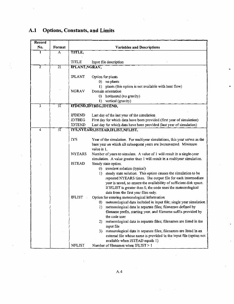
A.I Options, Constants, and Limits

RecordNo.

1

2

3

4

FormatA

21

31

51

Variables and DescriptionsTITLE,

TITLE Input file descriptionIPLANT,NGRAV,

IPLANT Option for plants0) no plants1) plants (this option is not available with heat flow)

NGRAV Domain orientation0) horizontal (no gravity)1) vertical (gravity)

IFDEND,IDTBEG,IDTEND,

IFDEND Last day of the last year of the simulationIDTBEG First day for which data have been provided (first year of simulation)IDTEND Last day for which data have been provided (last year of simulation)IYS,NYEARS,ISTEAD,IFLIST,NFLIST,

IYS Year of the simulation. For muitiyear simulations, this year serves as thebase year on which all subsequent years are incremented. Minimumvalue is 1.

N YEARS Number of years to simulate. A value of 1 will result in a single-yearsimulation. A value greater than 1 will result in a muitiyear simulation.

ISTEAD Steady state option.0) transient solution (typical)1) steady state solution. This option causes the simulation to be

repeated NYEARS times. The output file for each intermediateyear is saved, so ensure the availability of sufficient disk space.If IFLIST is greater than 0, the code uses the meteorologicaldata from the first year files only.

IFLIST Option for entering meteorological information0) meteorological data included in input file; single year simulation1) meteorological data in separate files; filenames defined by

filename prefix, starting year, and filename suffix provided bythe code user

2) meteorological data in separate files; filenames are listed in theinput file

3) meteorological data in separate files; filenames are listed in anexternal file whose name is provided in the input file (option notavailable when ISTEAD equals I)

NFLIST Number of filenames when IFLIST > 1

A.4

RecordNo.

5

6

7

Format21

3I,R

3R

Variables and DescriptionsNPRINT,STOPHR,

NPRINT Option for level of output0) Daily summaries and end-of-simulation summary1) DELSUB and daily summaries and end-of-simulation summary.

Use of this option may result in large *.RES output files ifIDTEND-NDAY is large:

STOPHR Stopping time when IDAY equals IDTEND and NPRINT equals 1. Thisfeature is useful for stopping a simulation at a time other than the end ofa day. A particular instance for using STOPHR would be for simulatinga time period less than a day. A normal value of STOPHR is 24. (units:hr)

ISMETH,INMAX,ISWDIF,DMAXBA,

ISMETH Option for method of solution0) Crank-Nicholson (standard method of previous versions of

UNSAT-H)1) Modified Picard iteration

INMAX Number of iterations allowed for solving the water flow equation. Avalue of 2 is the minimum allowed. INMAX steps will be taken ifDHTOL=0.

ISWDIF Option for time step control0) Check all nodes to see if the relative change in THETA of every

node is less than DMAXBA1) Reduce the time step if the mass balance for the whole profile

exceeds DMAXBADMAXBA Time step control parameter. If ISWDIF = 0, DMAXBA is the

maximum allowable relative change in the water content of any node[suggested value is 0.01 (no units)]. If ISWDIF equals 1, DMAXBA isthe maximum allowable mass balance error (units: cm)

DELMAX,DELMIN,OUTTIM,

DELMAX Maximum allowable time step, normally 1 hr. The value of DELMAXmust be less than or equal to OUTTIM, otherwise DELMAX is set equalto OUTTIM (units: hr)

DELMIN Minimum allowable time step. The value must be less than or equal toDELMAX. (units: hr)

OUTTIM Determines the size of the DELSUB period, which is used to divide eachday into equal increments for calculations; if NPRINT equals 1,OUTTIM is also the time interval for generating output. If equal to zero,OUTTIM is reset to the DELMAX value (in which case, the followingOUTTIM restrictions apply to the DELMAX value). For values ofOUTTTM greater than 1.0, 24/OUTTIM must produce an integer value.Values cannot be greater than 24. For values of OUTTIM less than 1.0,1.0/OUTTIM must produce an integer value if using hourly precipitationand evaporation data, (units: hr)

A.5

RecordNo. Format Variables and Descriptions

5R RFACT,RAINIF,DHTOL,DHMAX,DHFACT,

RFACT

RAINIF

DHTOL

Maximum time-step factor. The time step can potentially be increasedby this factor following the completion of a successful time step.Rainfall time-step reduction factor. At the start of water applicationevent, the time step will be reduced by the RAINIF factor.Iteration control parameter. If the relative change in head during aniteration

hj -hj

•DHMAX

DHFACT

exceeds DHTOL, the time step is reduced by half. If the value ofDHTOL is 0, then this control parameter is not used, (units: cm)Iteration control parameter. If DHMAX is positive, each potential headsolution is checked to see if the change in head

hJ-hJ'1

exceeds DHMAX. If so, the time step size is reduced by the factorDHFACT and re-solved, (units: cm)Time step reduction factor if DHMAX > 0.

2I,R KOPT,KEST,WTF,

KOPT Options for describing the soil hydraulic properties1) Polynomial2) Haverkamp (Haverkamp etal. 1977)3) Brooks-Corey (Corey 1977)4) van Genuchten (van Genuchten 1978)5) Modified Brooks-Corey (Fayer and Simmons 1995)6) Modified van Genuchten (Fayer and Simmons 1995)7) Rossi and Nimmo "sum" model (Rossi and Nimmo 1994)8) Rossi and Nimmo "junction" model (Rossi and Nimmo 1994)

KEST Option for estimating the liquid conductivity at the midpoint betweennodes

1) Arithmetic mean with an option for upstream weighting (seeWTF)

2) Harmonic mean3) Geometric mean

WTF Weighting factor (from 0.0 to 1.0) used to weight the conductivity of theupstream node in the calculation of conductivities between nodes. Avalue of 0.5 weights the nodes equally. WTF applies only when KEST is1.

A.6

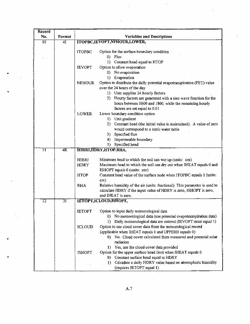
RecordNo.10

11

12

Format41

4R

31

Variables and DescriptionsITOPBC,IEVOPT,NFHOUR,LOWER,

ITOPBC Option for the surface-boundary condition0) Flux1) Constant head equal to HTOP

IEVOPT Option to allow evaporation0) No evaporation1) Evaporation

NFHOUR Option to distribute the daily potential evapotranspiration (PET) valueover the 24 hours of the day

1) User supplies 24 hourly factors2) Hourly factors are generated with a sine wave function for the

hours between 0600 and 1800, while the remaining hourlyfactors are set equal to 0.01

LOWER Lower boundary condition option1) Unit gradient2) Constant head (the initial value is maintained). A value of zero

would correspond to a static water table3) Specified flux4) Impermeable boundary5) Specified head

HIRRI,HDRY,HTOP,RHA,

HIRRI Minimum head to which the soil can wet up (units: cm)HDRY Maximum head to which the soil can dry out when IHEAT equals 0 and

ISHOPT equals 0 (units: cm)HTOP Constant head value of the surface node when ITOPBC equals 1 (units:

cm)RHA Relative humidity of the air (units: fractional). This parameter is used to

calculate HDRY if the input value of HDRY is zero, ISHOPT is zero,and IHEAT is zero.

IETOPT,ICLOUD,ISHOPT,

IETOPT Option to input daily meteorological data0) No meteorological data (use potential evapotranspiration data)1) Daily meteorological data are entered (IEVOPT must equal 1)

ICLOUD Option to use cloud cover data from the meteorological record(applicable when IHEAT equals 1 and UPPERH equals 0)

0) No. Cloud cover calculated from measured and potential solarradiation

1) Yes, use the cloud cover data providedISHOPT Option for the upper surface head limit when IHEAT equals 0

0) Constant surface head equal to HDRY1) Calculate a daily HDRY value based on atmospheric humidity

(requires IETOPT equal 1)

A.7

RecordNo.13

14

15

FormatI,R

I,3R,A

2I,R

Variables and DescriptionsIRAIN,HPR,

IRAIN Option for water application information0) Enter hourly precipitation data (see Boundary Condition

section)1) Use the daily precipitation values that are included with the

meteorological data and apply at the HPR rate.HPR Hourly precipitation rate when IETOPT equals 1. Starting at 0000 hr,

precipitation is applied at the HPR rate until the amount to be applied isless than the amount that would fall in one hour at the HPR rate, afterwhich the remainder is applied over the next hour. The default value is1.0 cm/hr (units: cm/hr)

IH YS, AIRTOL,HYSTOL,H YSMXH,HYFILE,

IHYS Option for hysteresis (only uses the van Genuchten soil water retentionfunction, KOPT=4)

0) no hysteresis1) hysteresis, starting on the primary drainage path2) hysteresis, starting on the primary sorption path3) hysteresis, starting on the main drainage path4) hysteresis restart, using hysteresis information from file with

extension "HRI" that was created during previous hysteresissimulation

AIRTOL Tolerance limit on entrapped air content below which volumetric aircontent is considered zero in hysteresis simulations (units: cm3/cm3)

HYSTOL Tolerance limit on head changes below which a change in head does nottrigger a path reversal during hysteresis simulations (units: cm)

HYSMXH Maximum head value for all materials above which hysteresis does notoccur. Used to avoid large changes in the head value of the surface node(units: cm)

HYFILE Name of restart file when IHYS equals 1; place no extra characters orcomments after the filename.

IHEAT,ICONVH,DMAXHE,

IHEAT Option for simulating heat flow0) No heat flow1) Heat flow (this option is not available with the plant option)

ICONVH Option to allow convective heat flow via water flow0) No convective heat flow allowed1) Convective heat flow allowed. Use caution when solving

convection-dominated problems because there is no upstreamweighting. Precipitation temperature depends on the value ofUPPERH: if 0, TA; if 1 or 2, TS; if 3, TSMEAN (units: J/m2)

DMAXHE Time step control parameter when greater than zero and IHEAT=1.Represents the maximum allowable heat balance error (units: J/m2)

A.8

RecordNo.16

17

18

19

FormatI,3R

1,2R

I,3R

21

Variables and DescriptionsUPPERH,TSMEAN,TSAMP,QHCTOP,

UPPERH Option for the upper boundary condition for heat flow0) Flux that is calculated based on weather and soil parameters1) Constant temperature (specified in initial conditions)2) Variable temperature (must specify TSMEAN and TAMP)3) Specified heat flux (must specify QHCTOP). Any convective

flow (e.g., heat associated with precipitation) will be added toQHCTOP. The water temperature will be set to TSMEAN.

TSMEAN Daily mean surface temperature when UPPERH equals 2; temperature ofinfiltrating water when UPPERH equals 3 (units: K)

TSAMP Daily surface temperature amplitude about TSMEAN when UPPERHequals 2 (units: K)

QHCTOP User-specified surface heat flux when UPPERH equals 3(units: J s'1 m"2)

LOWERH,QHLEAK,TGRAD,

LOWERH Option for the lower boundary condition for heat flow1) Temperature gradient (must specify TGRAD).2) Constant temperature (specified in initial conditions). Can

specify TGRAD.3) Constant heat flux (must specify QHLEAK). TGRAD is not

used.QHLEAK Heat flux at the bottom boundary when LOWERH equals 3

(units: J hr'1 cm'2)TGRAD Temperature gradient at the bottom boundary when IHEAT equals 1 and

LOWERH equals 1. A positive value indicates an upward gradientbecause depth is positive downward (units: K/cm)

IVAPOR,TORT,TSOIL,VAPDIF,

I VAPOR Option to allow vapor flow. If chosen, values must be supplied forTORT, TSOIL, and VAPDIF. If IHEAT=1, vapor can diffuse across thebottom boundary in response to a temperature gradient (TGRAD) ifLOWERH equals 1 (temperature gradient boundary) or 2 (constanttemperature boundary).

0) No, vapor flow not allowed1) Yes, vapor flow allowed

TORT TortuosityTSOIL Average temperature of the soil for use in calculations of isothermal

vapor flow (units: K)VAPDIF Diffusion coefficient of vapor in air (units: cm2/s)

MATN,NPT,

MATN Number of different soil materialsNPT Number of nodes

A.9

RecordNo.20

Format4(I,R)

per line

Variables and DescriptionsMAT,Z,

MAT Soil material identification number for the given nodeZ Depth of node below the surface (units: cm)

Repeat Record 20 until MATN nodes defined

A.10

A.2 Soil Property Information

IF KOPT = 1 (polynomial description) THENRecord

No.1

2

3

4

5

6

7

Format21

A

I,2R

2I,2R

5R

A

I,2R

Variables and DescriptionsMAXPOL,MAXCOE,

MAXPOL Maximum number of polynomials for any given soil hydraulicproperty function (limited to M2 in unsath. inc)

MAXCOE Maximum number of polynomial coefficients per soil hydraulicproperty function (MAXPOL*MAXCOE is limited to M4 inunsath. inc)

DUMMY,

DUMMY Dummy title that can be used to describe the soil type andindicate that what follows are water retention parameters

NSUBTH,AIRINT,THET,

NSUBTH Number of subdivisions of the water retention curve for thatparticular material

AIRINT Air entry head (units: cm)THET Saturated water content (units: cm3/cm3)II,NDEGTH,XX,XDIVTH,

II Index of the water retention polynomialNDEGTH Number of polynomial coefficients, or polynomial degree + 1XX Minimum head for which the given polynomial applies

(units: cm)XDIVTH Maximum head for which the given polynomial applies

(units: cm).CREGTH,

CREGTH Polynomial coefficients for describing water retention; enterNDEGTH values of CREGTH

Repeat Records 4-5 NSUBTH timesDUMMY,

DUMMY Dummy title that can be used to describe the soil type andindicate that what follows are conductivity parameters

NSUBKH,AIRINK,SK,

NSUBKH Number of subdivisions of conductivity curve for that particularmaterial

AIRINK Air entry head (units: cm)SK Saturated hydraulic conductivity (units: cm/hr)

A.ll

RecordNo.

8

9

Format2I,2R

5R

Variables and DescriptionsII,NDEGKH,XX,XDIVKH,

II Index of the conductivity polynomialNDEGKH Number of polynomial coefficients, or polynomial degree + 1XX Minimum head for which the given polynomial applies

(units: cm)XDIVKH Maximum head for which the given polynomial applies

(units: cm)CREGKH,

CREGKH Polynomial coefficients for describing conductivity; enterNDEGKH values of CREGKH

Repeat Records 8-9 NSUBKH times

Repeat Records 2-9 MATN times

ENDIF(KOPT=1)

IF KOPT = 2 (Haverkamp functions) THENRecord

No.1

2

3

FormatA

6R

A

Variables and DescriptionsDUMMY,

DUMMY Dummy title that can be used to describe the soil type andindicate that what follows are water retention parameters

THET,THTR,AIRINT,ALPHA,BETA,RETOPT,

THET Saturated water content (units: cm3/cm3)THTR Residual water content (units: cm3/cm3)AIRINT Air entry head (units: cm)ALPHA Coefficient of Haverkamp function (Haverkamp et al. 1977)BETA Coefficient of Haverkamp functionRETOPT Retention option

1) function operates on head value2) function operates on ln(head) value

DUMMY,

DUMMY Dummy title that can be used to describe the soil type andindicate that what follows are conductivity parameters

A.12

RecordNo.4

Format4R

Variables and Descriptions

AIRINK,SK,A,B,

AIRINK Air entry head (units: cm)SK Saturated hydraulic conductivity (units: cm/hr)A Coefficient of Haverkamp functionB Coefficient of Haverkamp function

Repeat Records 1 -4 MATN times

ENDIF (KOPT = 2)

IF KOPT = 3 (Brooks-Corey functions) THENRecord

No.1

2

3

4

FormatA

4R

A

5R

Variables and DescriptionsDUMMY,

DUMMY Dummy title that can be used to describe the soil type andindicate that what follows are water retention parameters

THET,THTR,AIRINT,B,

THET Saturated water content (units: cmVcm3)THTR Residual water content (units: cmVcmOAIRINT Air entry head (units: cm)B Coefficient of Brooks-Corey function

DUMMY,

DUMMY Dummy title that can be used to describe the soil type andindicate that what follows are conductivity parameters

RKMOD,SK,AIRENK,B,EPIT,

RKMOD Conductivity model option:1) Burdine (Burdine 1953)2) Mualem (Mualem 1976)

SK Saturated hydraulic conductivity (units: cm/hr)AIRENK Air entry-head (units: cm)B Coefficient of Brooks-Corey functionEPIT Exponent of the pore interaction term. Values of 2 and 0.5 are

standard for the Burdine and Mualem models, respectively.

Repeat Records 1-4 MATN times

ENDIF (KOPT = 3)

A.13

IF KOPT = 4 (van Genuchten functions) THENRecord

No.1

2

3

4

FormatA

4R

A

5R

Variables and DescriptionsDUMMY,

DUMMY Dummy title that can be used to describe the soil type andindicate that what follows are water retention parameters

THET,THTR,VGA,VGN,

THET Saturated water content (units: cm3/cm;')THTR Residual water content (units: cm3/cm'>)VGA Coefficient a of the vain Genuchten function (units: I/cm)VGN Coefficient n of the van Genuchten function (no units)DUMMY,

DUMMY Dummy title that can be used to describe the soil type andindicate that what follows are conductivity parameters

RKMOD,SK,VGA,VGN,EPIT,

RKMOD Conductivity model options1) Burdine (« = 1-2/w)2) Mualem (m= l-l/n)

SK Saturated hydraulic conductivity (units: cm/hr)VGA Coefficient a of the van Genuchten function (units: I/cm)VGN Coefficient n of the van Genuchten function (no units)EPIT Exponent of the pore interaction term. Values of 2 and 0.5 are

standard for the Burdine and Mualem models, respectively (nounits)

Repeat Records 1-4 MATN times

ENDIF (KOPT = 4)

IF KOPT = 5 (modified Brooks-Corey functions) THENRecord

No.1

2

FormatA

5R

Variables and DescriptionsDUMMY,

DUMMY Dummy title that can be used to describe the soil type andindicate that what follows are water retention parameters

THET,THTA,AIRINT,B,HM,

THET Saturated water content (units: cm3/cmi>)THTA Transition water content (units: cm3/cmJ)AIRINT Air entry head (units: cm)B Coefficient equal to inverse of Brooks-Corey X parameterHM Suction head corresponding to zero water content (units: cm)

A.14

RecordNo.

3

4

FormatA

Variables and DescriptionsDUMMY,

DUMMY Dummy title that can be used to describe the soil type andindicate that what follows are conductivity parameters

SK,EPIT,

SK Saturated hydraulic conductivity (units: cm/hr)EPIT Exponent of the pore interaction term. A value of 0.5 is .

standard for the Mualem model.

Repeat Records 1-4 MAIN times

ENDIF (KOPT = 5)

IF KOPT = 6 (modified van Genuchten functions) THENRecord

No.I

2

3

4

FormatA

5R

A

2R

Variables and DescriptionsDUMMY,

DUMMY Dummy title that can be used to describe the soil type andindicate that what follows are water retention parameters

THET,THTA,VGA,VGN,HM,

THET Saturated water content (units: cm3/cm3)THTA Transition water content (units: cm3/cmJ)VGA Coefficient similar to van Genuchten a (units: I/cm)VGN Coefficient similar to van Genuchten n (no units)HM Suction head corresponding to zero water content (units: cm)DUMMY,

DUMMY Dummy title that can be used to describe the soil type andindicate that what follows are conductivity parameters

SK,EPIT,

SK Saturated hydraulic conductivity (units: cm/hr)EPIT Exponent of the pore interaction term (no units). A value of

0.5 is standard for the Mualem model.

Repeat Records 1-4 MATN times

ENDIF (KOPT = 6)

A.15

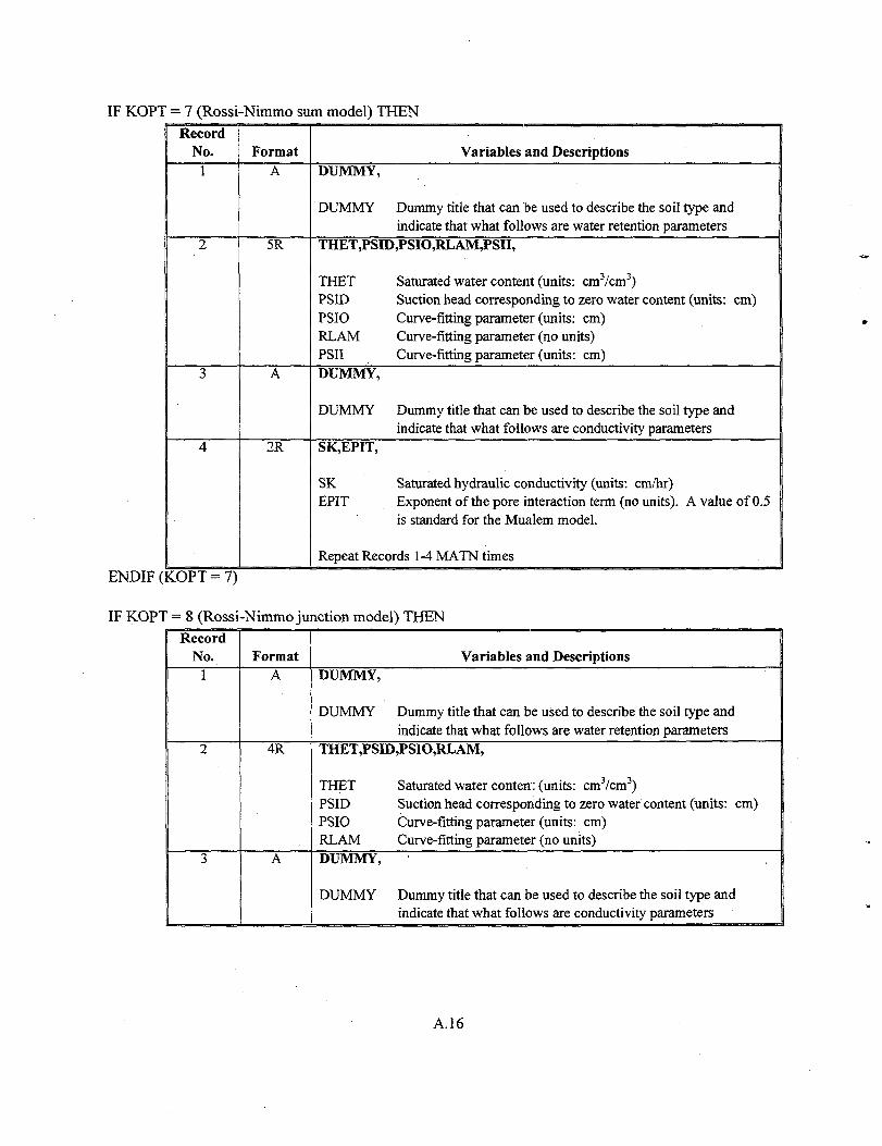
IF KOPT = 7 (Rossi-Nimmo sum model) THENRecord

No.1

2

3

4

FormatA

5R

A

2R

Variables and DescriptionsDUMMY,

DUMMY Dummy title that can be used to describe the soil type andindicate that what follows are water retention parameters

THET,PSID,PSIO,RLAM,PSII,

THET Saturated water content (units: cnvVcm3)PSID Suction head corresponding to zero water content (units: cm)PSIO Curve-fitting parameter (units: cm)RLAM Curve-fitting parameter (no units)PSII Curve-fitting parameter (units: cm)

DUMMY,

DUMMY Dummy title that can be used to describe the soil type andindicate that what follows are conductivity parameters

SK,EPIT,

SK Saturated hydraulic conductivity (units: cm/hr)EPIT Exponent of the pore interaction term (no units). A value of 0.5

is standard for the Mualem model.

Repeat Records 1 -4 MATN times

ENDIF (KOPT = 7)

IF KOPT = 8 (Rossi-Nimmo junction model) THENRecord

No.1

2

3

FormatA

4R

A

Variables and DescriptionsDUMMY,

DUMMY Dummy title that can be used to describe the soil type andindicate that what follows are water retention parameters

THET,PSID,PSIO,RLAM,

THET Saturated water content (units: cm3/cm3)PSID Suction head corresponding to zero water content (units: cm)PSIO Curve-fitting parameter (units: cm)RLAM Curve-fitting parameter (no units)DUMMY,

DUMMY Dummy title that can be used to describe the soil type andindicate that what follows are conductivity parameters

A.16

RecordNo.4

Format2R

Variables and DescriptionsSK,EPIT,

SK Saturated hydraulic conductivity (units: cm/hr)EPIT Exponent of the pore interaction term (no units). A value of 0.5

is standard for the Mualem model.

Repeat Records 1-4 MATN times

ENDIF(KOPT = 8)

IF IHYS = 1 (Hysteresis properties) THENRecord

No.1

2

FormatA

I,3R

Variables and DescriptionsDUMMY,

DUMMY Dummy title that can be used to describe the soil type andindicate that what follows are soil-specific hysteresis parameters

IPATHA,SARWA,ALFACT,HYSHPH,

IPATHA Maximum number of hysteretic paths (suggested value = 7)SARWA Maximum entrapped air content (units: cm /cm")ALFACT Factor that relates the imbibition a,- to the desorption ad.

Typical value is 2.0. The value must be greater than or equal toCCj.

HYSHPH Soil-specific maximum suction head above which hysteresis isnot operable (units: cm). If HYSHPH less than or equal to zero,or greater than HYSMXH (the global limit), the HYSHPH valuefor that material is reset to HYSMXH.

Repeat Records 1-2 MATN times

ENDIF (IHYS = 1)

IF IHEAT = 1 (Thermal properties) THENRecord

No.1

FormatA

Variables and DescriptionsDUMMY,

DUMMY Dummy title that can be used to describe the soil type andindicate that what follows are soil-specific thermal conductivityand heat capacity parameters. Coefficients for the thermalconductivity equation can be found in Cass et al. (1984).

A.17

RecordNo.

2

3

4

Format

6R

A

5R

Variables and DescriptionsTCON(1:5),CHS,

TCON(l) Thermal conductivity (kh) coefficient a, where

kh = a + b(0/0s)+(a-d)cx^[-c(0/0sf]TCON(2) Thermal conductivity coefficient bTCON(3) Thermal conductivity coefficient cTCON(4) Thermal conductivity coefficient dTCON(5) Thermal conductivity coefficient eCHS Volumetric heat capacity of the soil particles (units: J cm'3 K"1)

DUMMY,

DUMMY Dummy title that can be used to describe the soil type andindicate that what follows are soil-specific parameters thatdefine the vapor flow enhancement factor. Coefficients for theenhancement factor equation can be found in Cass et al. (1984)

EF(1:5),

EF( 1) Enhancement factor (77) coefficient a, where

r) = a + b(0l0s)+(a-d) exp[-c(<9 /ds)e]

EF(2) Enhancement factor coefficient bEF(3) Enhancement factor coefficient cEF(4) Enhancement factor coefficient dEF(5) Enhancement factor coefficient e

Note: To achieve an enhancement factor of 1.0 (i.e., no enhancement), setcoefficient a to 1.0 and b through e to zero.

Repeat Records 1-4 MATN times

ENDIF(IHEAT=1)

A.18

A.3 Initial Conditions

RecordNo.

1

2

FormatI

4Rper line

Variables and DescriptionsNDAY,

NDAY Day for which end-of-day suction head values are specified as initialconditions. For example, when NDAY = 0, the initial head values are forthe end of the day before simulation day 1. NDAY = 90 would indicatethat the initial head values are from the end of day 90 and will serve asinitial head values for day 91.

H(1...NPT),

H Initial suction head. Values must be less than or equal to HDRY whenIHEAT equals 0 (units: Cm)

IF IHEAT = 1Record

No.1

Format4R

per line

Variables and DescriptionsT(1...NPT),

T Initial soil temperature (units: K)

ENDIF (IHEAT = 1)

A.19

A.4 Plant Information

IF IPLANT = 1 (plant parameters) THENRecord

No.1

2

Format61

R

Variables and DescriptionsLEAF,NFROOT,NUPTAK,NFPET,NSOW,NHRVST,

LEAF Option for leaf area index (LAI)0) LAI values not needed (i.e., NFPET equals 2)1) User supplies LAI values for the year2) User supplies a subroutine (inoperative)

NFROOT Option for root growth1) Exponential relationship2) User supplies a subroutine (inoperative)

NUPTAK Option for plant water uptake1) Sink term approximation proposed by Feddes et al.

(1978). Requires values for HW,HD, and HN.2) User supplies a subroutine (inoperative)

NFPET Option for partitioning PET into transpiration (PT) andevaporation (PE) components

1) User supplies daily PET values and program partitionsit into PT and PE based on LAI and equation byRitchie and Burnett (1971)

2) User supplies daily PET values and program partitionsit into PT and PE based on the cheatgrass data of Hinds(1975)

NSOW Day of the year on which seeds germinate. Must be less thanday 91 or greater than day 273 when NFPET equals 2.

NHRVST Day of the year on which plants cease transpiring. Must bebetween days 151 and 243 when NFPET equals 2.

BARE,

BARE Fraction of soil surface that is bare of plants

IF LEAF = 1 (leaf area index)Record

No.1

2

FormatI

4(I,R)per line

Variables and DescriptionsNDLAI,

NDL AI Number of changes in the LAI relationship when LEAFequals 1

IDLAI,VLAI,

IDLAI Day of the year on which the LAI is changed to thecorresponding FLAI value

VLAI Leaf area index on the corresponding NGROW day

END (LEAF = 1)

A.20

IF NFROOT = 1 (root density and depth parameters)Record

No.1

2

Format3R

101per line

Variables and DescriptionsAA,B1,B2,

AA Coefficient a in the root growth equationRLD = a exp(-fe)+c

Bl Coefficient b in the root growth equationB2 Coefficient c in the root growth equation

NTROOT(1..NPT),

NTROOT Growth day on which roots reach the correspondingnode

ENDIF (NFROOT =1)IF NUPTAK = 1 (plant water uptake parameters)

RecordNo.

1Format

3RVariables and Descriptions

HW,HD,HN,

HW Head corresponding to water content below whichplants wilt and stop transpiring. HW must be less thanHDRY. (units: cm)

HD Head corresponding to water content below which planttranspiration starts to decrease (units: cm)

HN Head corresponding to water content above which plantsdo not transpire because of anaerobic conditions (units:cm)

Repeat Record 1 MATN times

ENDIF (NUPTAK =1)IF NFPET = 1 (partition PET using leaf area index)

RecordNo.

1Format

5RVariables and Descriptions

PETPC(1:5),

PETPC( 1) Coefficient a of Ritchie equation (=a+6LAF) (theoriginal values for a, b, and c were -0.21, 0.7, and 0.5;the new values, derived by Mark Ankeny from a re-analysis of the original data, are 0.0, 0.52, and 0.5)

PETPC(2) Coefficient b of Ritchie equationPETPC(3) Coefficient c of Ritchie equationPETPC(4) Lower limit of Ritchie equation (original value was 0.1)PETPC(5) Upper limit of Ritchie equation (original value was 2.7)

A.21

ELSE IF NFPET = 2 (partition PET using cheatgrass algorithm)

ENDIF (NFPET)ENDIF(IPLANT=1)

RecordNo.

1Format

RVariables and Descriptions

BIOMAS,

BIOMAS Plant shoot biomass scaling factor used in adjusting thetranspiration component of PET. The base value is220 g/m2. A lower value will result in lowertranspiration and higher evaporation, while a highervalue will result in higher transpiration and lowerevaporation (units: g/mz).

A.22

A.5 Boundary Conditions

IF ((IEVOPT = 1 OR IPLANT = 1) and IHEAT = 0) THENIF (NFHOUR = 1) THEN

ENDIF

RecordNo.

1Format

8Rper line

Variables and DescriptionsFPET(1:24),

FPET Hourly PET distribution factors. The 24 FPET factorsmust sum to 1.0

Note: Repeat Record 1 three times

ENDIF

IF IETOPT = 1 (Meteorological parameters)IF IHEAT = 0 (isothermal) THEN

RecordNo.

1Format

4RVariables and Descriptions

ALBEDO,ALT,ZU,PMB,

ALBEDO Potential evapotranspiration (units: cm/day)ALT Altitude of the site being simulated (units: m)ZU Height of the wind speed measurement (units: m)PMB Average annual atmospheric pressure (units: mb)

ELSE IF IHEAT=1 (thermal) THEN

ENDIFENDIF (IETOPT = 1 )

RecordNo.

1Format

4RVariables and Descriptions

ZH,ZM,ZT,ZU,D,LAT,

ZH Roughness length for heat transfer (units: m)ZM Roughness length for momentum transfer (units: m)ZT Height of air temperature measurement (units: m)ZU Height of the wind speed measurement (units: m)D Zero plane displacement height (units: m)LAT Latitude of the site being simulated (units: degrees)

A.23

IF LOWER = 3 (Lower boundary condition specified fluxes) THENRecord

No.1

2

FormatI

5(I,R)per line

Variables and DescriptionsNTLEAK,

NTLEAK Number of times the flux lower boundary condition changesduring the simulation period (limit is 50). Note that for daysbetween flux changes, the bottom flux will be interpolated.

NQLEAK,QLEAK,

NTLEAK Day on which the bottom boundary flux is changed to thecorresponding QLEAK value. Note that a QLEAK valuemust be specified for the first and last days of the simulation.

QLEAK Bottom boundary flux on the corresponding NQLEAK day(units: cm/day)

Repeat Record 2 until NTLEAK pairs of data have been entered

ENDIF(LOWER =IF LOWER = 5 (Lower boundary condition specified head) THEN

RecordNo.

1

2

FormatI

I,Rper line

Variables and DescriptionsINDEXB,

INDEXB Number of times the head lower boundary condition changesduring the simulation period (limit is 50). Note that for daysbetween head changes, the bottom head value will beinterpolated.

BBHEAD(1:2),

BBHEAD(l) Day on which the bottom boundary head is changed. Notethat a BBHEAD value must be specified for the first andlast days of the simulation (units: d, i.e., 0600 h on day310 is entered as 310.25)

BBHEAD(2) Bottom boundary head on the corresponding BBHEAD(l)day (units: cm)

Repeat Record 2 until INDEXB pairs of data have been entered

ENDIF (LOWER = 5)

A.24

IF IFLIST = 0 (meteorological data included with input file) THENIF IETOPT = 0 (PET values) THEN

RecordNo.

1Format

8Rper line

Variables and DescriptionsPET(1:IDEND),

PET Potential evapotranspiration (units: cm/day)

ELSE IF IETOPT = 1 (daily meteorological data) THENRecord

No.1

Format8R

Variables and DescriptionsMEDAT(1:8),

RMDATA( 1, J) Day of the year for which the following dataapply

RMDATA(2,J) Maximum air temperature (units: °F)RMDATA(3,J) Minimum air temperature (units: °F)RMDATA(4,J) Dew point temperature (units: °F)RMDATA(5,J) Solar radiation (units: langleys)RMDATA(6,J) Average wind speed (units: miles/hr)RMDATA(7,J) Average cloud cover (units: tenths)RMDATA(8,J) Precipitation (units: inches)

Repeat Record 5 for each day of the year.

ENDIFIF (IRAIN = 0) THEN

RecordNo.

1

2

FormatI

3I,R

Variables and DescriptionsNWATER,

NWATER Total number of days during which there is waterapplication

IRDAY,ERTYPE,NP,EFICEN,

IRDAY Day on which a water application event occursIRTYPE Option for type of water application

1) rainfall2) irrigation3) constant ponding depth less than 1 day4) constant ponding depth greater than 1 day

NP Number of times during the day that the waterapplication rate changes

EFICEN Efficiency of the irrigation scheme (i.e., how much ofthe water actually gets onto the soil surface)

A.25

RecordNo.

3Format

2Rper line

Variables and DescriptionsRTIME,AMOUNT,

RTIME Time of day when the water application rate changes(use hours only) (units: hr). The exception is whenIRTYPE equals 4, and then the units are days. IfIRTYPE equals 4 and RTIME(NP) equals 0, pondingcontinues for the remainder of the simulation (untilDAYEND).

AMOUNT When IRTYPE equals 1 or 2, AMOUNT is therainfall/irrigation amount that falls until the next ratechange, [RTIME(I+1)]; when IRTYPE equals 3 or 4,AMOUNT is the depth of water ponded on the surface(units: cm).

Note: Repeat Record 3 NP timesNote: Repeat the sequence of Records 2 and 3 N WATER times

ENDIF (IRAIN = 0)ELSE IF IFLIST = 1 (meteorological data in separate files; filenames provided in input file) THEN

RecordNo.

1

2

3

FormatA

A

A

Variables and DescriptionsDIRLOC,

DIRLOC Directory name within which resides the filescontaining PET or meteorological data. The file namessimilar except for their year designation (e.g.,filpre9999.dat)

FELPRE,

FILPRE Common filename prefix (e.g., Jllpre9999.dat)FILEXT,

FILEXT Common filename extension (e.g., filpre9999.di<tf)

IF IRAIN = 0 (precipitation data provided separate from meteorological data)Record

No.1

2

FormatA

A

Variables and DescriptionsDIRLOC,

DIRLOC Directory name within which resides the filescontaining precipitation data. The file names similarexcept for their year designation (e.g., filpre9999.dat)

FILPRE,

FILPRE Common filename prefix (e.g.,./7//ve9999.dat)

A.26

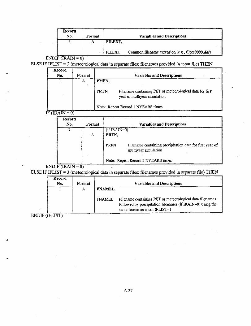
RecordNo.

3

F(IRAIN = 0)

FormatA FILEXT,

FILEXT

Variables and Descriptions

Common filename extension (e.g., filpre9999.tfa/)

ENDI

ELSE IF IFLIST = 2 (meteorological data in separate files; filenames provided in input file) THEN

RecordNo.

1Format

AVariables and Descriptions

PMFN,

PMFN Filename containing PET or meteorological data for firstyear of multiyear simulation

Note: Repeat Record 1 NYEARS times

IF (IRAIN = 0)Record

No.2

Format

A

Variables and Descriptions(ifIRAIN=0)PRFN,

PRFN Filename containing precipitation data for first year ofmultiyear simulation

Note: Repeat Record 2 NYEARS times

ENDIF (IRAIN = 0)ELSE IF IFLIST = 3 (meteorological data in separate files; filenames provided in separate file) THEN

ENDIF (IFLIST)

RecordNo.

1Format

AVariables and Descriptions

FNAMEL,

FNAMEL Filename containing PET or meteorological data filenamesfollowed by precipitation filenames (if IRAIN=0) using thesame format as when IFLIST=1

A.27

A.6 References

BurdineNT. 1953. "Relative permeability calculation from size distribution data." Petr. Trans., Am.Inst. MiningMetall. Eng. 198:71-77.

Cass A., GS Campbell, and TL Jones. 1984. "Enhancement of thermal water vapor diffusion in soil."SoilSci. Soc. Am. J. 48:25-32.

Celia MA, ET Bouloutas, and RL Zarba. 1990. "A general mass-conservative numerical solution for theunsaturated flow equation." Water Resour. Res. 26:1483-1496.

Corey AT. 1977. Mechanics of Heterogeneous Fluids in Porous Media. Water Resources Publications,Fort Collins, Colorado.

Fayer MJ and CS Simmons. 1995. "Modified soil water retention functions for all matric suctions,"Water Resour. .Res. 31:1233-1238.

Feddes RA, PJ Kowalik, and H Zaradny. 1978. Simulation of Field Water Use and Crop Yield. JohnWiley and Sons, Inc., New York.

Haverkamp R, M Vaclin, J Touma, PJ Wierenga, and G Vachaud. 1977. "A comparison of numericalsimulation models for one-dimensional infiltration." Soil Sci. Soc. Am. J. 41:285-294.

Hinds WT. 1975. "Energy and carbon balances in cheatgrass: An essay in autecology." EcologicalMonogr. 45:367-388.

Lenhard RJ, JC Parker, and JJ Kaluarachchi. 1991. "Comparing simulated and experimental hysteretictwo-phase transient fluid flow phenomena." Water Resour. Res. 27:2113-2124.

Mualem Y. 1976. "A new model for predicting the hydraulic conductivity of unsaturated porous media."Water Resour. Res. 12(3):513-522.

Ritchie JT, and E Burnett. 1971. "Dryland evaporative flux in a subhumid climate, 2, plant influences."Agron.J. 63:56-62.

Rossi C and JR Nimmo. 1994. "Modeling of soil water retention from saturation to oven dryness."Water Resour. Res. 30, 701-708.

van Genuchten R. 1978. Calculating the unsaturated hydraulic conductivity with a new closed-formanalytical model. Water Resource Program, Department of Civil Engineering, Princeton University,Princeton, New Jersey.

A.28

Appendix B

Input and Output Files for Example Simulations

Appendix B

Input and Output Files for Example Simulations

Figure B.I. Input File for Clay Infiltration Simulation

CLAY.INP: test simulation0,1,50,1,50,1,1,0,0,1,0,24.0,0,2,1,1.0E-4,0.15,1.0E-04,0.0,2.0,1.0E-05,0.0,0.0,0.0,2,3,0,1,0,2,2,0.0,2.0E+04,0.0,0.0,0,0,0,0,0,0,0,0,0,0,0,0,0,0,0,0,0,0,0.0,0.0,0,0.66,288.46,0.24,1,250,1, 0.0,1, 1.0,1,1, 4.0,1, 5.0,1,

IPLANT,NGRAVIFDEND,IDTBEG, IDTENDIYS,NYEARS, ISTEAD,IFLIST,NFLISTNPRINT,STOPHRISMETH,INMAX, ISWDIF,DMAXBADELMAX,DELMIN, OUTTIMRFACT,RAINIF, DHTOL,DHMAX,DHFACTKOPT,KEST,WTFITOPBC,IEVOPT, NFHOUR,LOWERHIRRI,HDRY,HTOP,RHAIETOPT,ICLOUD, ISHOPTIRAIN,HPRIHYS,AIRTOL,HYSTOL,HYSMXH,HYFILEIHEAT,ICONVH,DMAXHEUPPERH,TSMEAN, TSAMP,QHCTOPLOWERH,QHLEAK, TGRADIVAPOR,TORT, TSOIL,VAPDIF

MATN,NPT2.0,1, 3.06.0,1, 7.0

1, 8.0,1, 9.0,1, 10.0,1, 11.0< similar lines deleted >1,240.0,1,241.0,1,242.0,1,243.01,24 4.0,1,245.0,1,24 6.0,1,247.01,248.0,1,249.0Yolo Light Clay Moisture Characteristic0.4 95,0.124,1.0,739.0,4.0,2.0,Yolo Light Clay Hydraulic Conductivity0.0,4.428E-02,124.6,1.77,0,600.0, 600.0,600.0,600.0,600.0,600.0,600.0,600.0,< similar lines deleted >600.0,600.0,600.0,600.0,600.0,600.0,600.0,600.0,600.0/600.0,0, NWATER

THET,THTR,AIRINT,A,B,RETOPT

AIRINK,SK,A,BNDAY

B.I

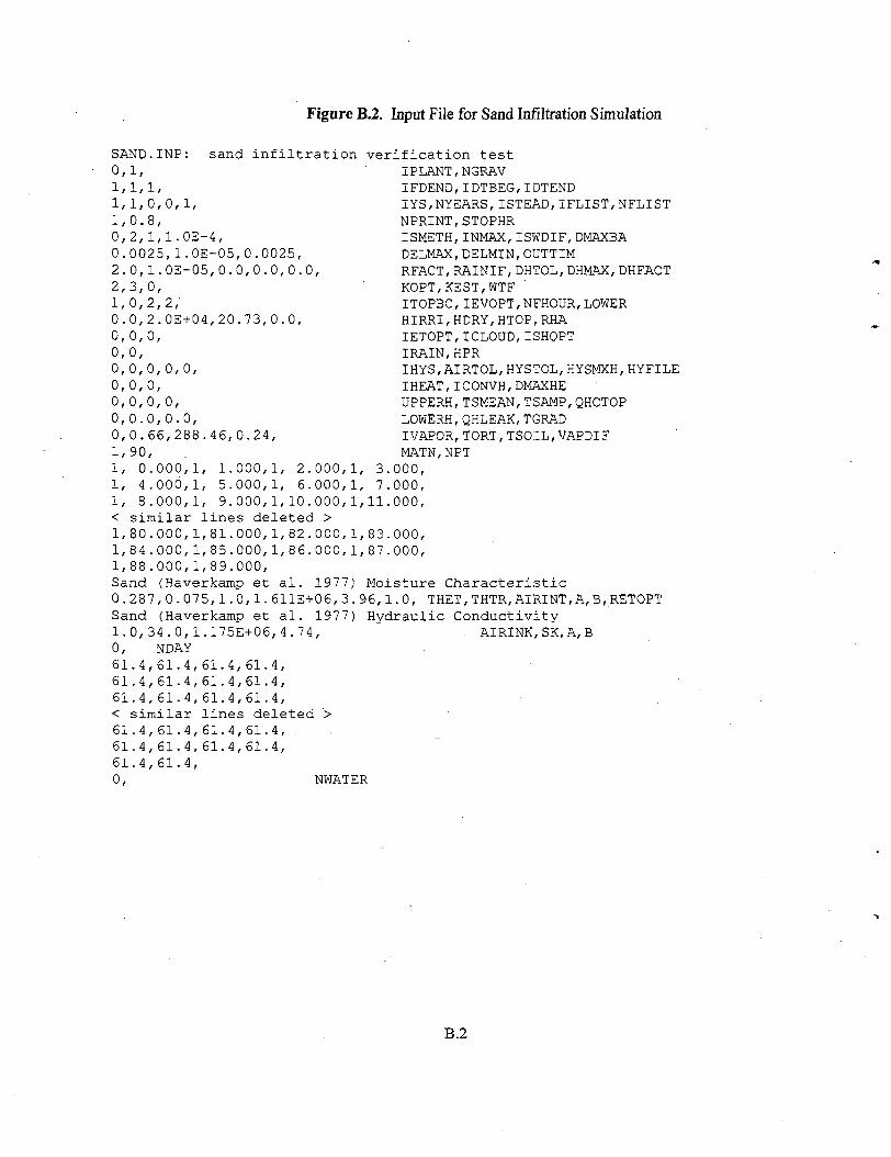
Figure B.2. Input File for Sand Infiltration Simulation

SAND.INP:0,1,1,1,1,1,1,0,0,1,1,0.8,0,2,l,1.0E-4,0.0025,1.0E-05,0.0025,2.0,1.0E-05,0.0,0.0,0.0,2,3,0,1,0,2,2,0.0,2.0E+04,20.73,0.0,0,0,0,0,0,0,0,0,0,0,0,0,0,0,0,0,0,0,0.0,0.0,0,0.66,288.46,0.24,1,90,1, 0.000,1, 1.000,1

sand infiltration verification testIPLANT,NGRAVIFDEND,IDTBEG,IDTENDIYS,NYEARS,ISTEAD,IFLIST,NFLISTNPRINT,STOPHRISMETH,INMAX,ISWDIF,DMAXBADELMAX,DELMIN,OUTTIMRFACT,RAINIF,DHTOL,DHMAX, DHFACTKOPT,KEST,WTFITOPBC,IEVOPT,NFHOUR,LOWERHIRRI,HDRY,HTOP,RHAIETOPT,ICLOUD,ISHOPTIRAIN,HPRIHYS,AIRTOL,HYSTOL,HYSMXH,HYFILEIHEAT,ICONVH,DMAXHEUPPERH,TSMEAN,TSAMP,QHCTOPLOWERH,QHLEAK,TGRADIVAPOR, TORT,TSOIL,VAPDIFMATN,NPT

2.000,1, 3.000,1, 4.000,1, 5.000,1, 6.000,1, 7.000,1, 8.000,1, 9.000,1,10.000,1,11.000,< s i m i l a r l i n e s d e l e t e d >1 , 8 0 . 0 0 0 , 1 , 8 1 . 0 0 0 , 1 , 8 2 . 0 0 0 , 1 , 8 3 . 0 0 0 ,1 , 8 4 . 0 0 0 , 1 , 8 5 . 0 0 0 , 1 , 8 6 . 0 0 0 , 1 , 8 7 . 0 0 0 ,1 ,88 .000 ,1 ,89 .000 ,Sand (Haverkamp et al. 1977) Moisture Characteristic0.287,0.075,1.0,1.611E+06,3.96,1.0, THET,THTR,AIRINT,A,B,RETOPTSand (Haverkamp et al. 1977) Hydraulic Conductivity1.0,34.0,1.175E+06,4.74, . AIRINK,SK, A, B0, NDAY61.4,61.4,61.4,61.4,61.4,61.4,61.4,61.4,61.4,61.4,61.4,61.4,< similar lines deleted >61.4,61.4,61.4,61.4,61..4,61.4,61.4,61.4,61.4,61.4,0, NWATER

B.2

Figure B3. Output File for Clay Infiltration Simulation

UNSAT-H Version 3.00INITIAL CONDITIONS

Input Filename:Results FilenameDate of Run:Time of Run:Title:CLAY.INP: test simulation

/filesO/home/mj_fayer/TESTV30/WEBV30/QA/clay.inp/filesO/home/mj_fayer/TESTV30/V_7JAN2000/QA/clay.res30 Dec 199909:38:07.95

NODE

135

DEPTH(cm)

0.000E+002.000E+004.000E+00

< similar lines245247249

2.440E+022.460E+022.480E+02

Initial

HEAD(cm)

0.000E+006.000E+026.000E+02

deleted >6.000E+026.000E+026.000E+02

Conditions

THETA(vol.)

0.23760.23760.2376

0.23760.23760.2376

TEMP(K)

0.000.000.00

0.000.000.00

NODE

246

246248250

DEPTH(cm)

1.000E+003.000E+005.000E+00

2.450E+022.470E+022.490E+02

Initial

HEAD(cm)

6.000E+026.000E+02•6.000E+02

6.000E+026.000E+026.000E+02

Conditions

THETA(vol.)

0.23760.23760.2376

0.23760.23760.2376

TEMP(K)

0.000.000.00

0.000.000.00

Initial Water Storage = 59.1619 cm

DAILY SUMMARY: Day = 1, Simulated Time = 24.0000 hr

Node NumberDepth (cm)Water (cm3/cm3)Head (cm)

0.0.

10000049500

240

25.00000.24218

. 490

50.00000.23760

740

75.00000.23760

10099.000000.23760

= 0.00000E+00 5.47605E+02 6.00000E+02 6.00000E+02 6.00000E+02LiqWater Flow (cm)= 3.89726E+00 6.41037E-03 1.59939E-03 1.59939E-03 1.59939E-03

LIQUIDPRESTOR INFIL RUNOFF EVAPO TRANS DRAIN59.1619+ 4.0260+ 0.0000 - 0.0000- 0.0000- 0.0016 =

NEWSTOR STORAGE63.1862 vs. 63.1831

Mass Balance = 3.1711E-03 cm; Time step attempts = 241 and successes = 209

DAILY SUMMARY: Day = 50-, Simulated Time = 24.0000 hr

Node NumberDepth (cm)Water (cm3/cm3]Head (cm)

00

1.00000.49500

240

25.00000.49500

5049.000000.49500

7574.000000.49500

10099.000000.49500

= 0.00000E+00 1.86395E-01 4.00284E-01 6.55896E-01 9.87959E-01

B.2

LiqWater Flow (cm)= 1.07098E+00 1.07098E+00 1.07098E+00 1.07098E+00 1.07098E+00

LIQUIDPRESTOR INFIL RUNOFF EVAPO TRANS DRAIN.118.5069+ 1.0710+ 0.0000 - 0.0000- 0.0000- 0.1992

Mass Balance = 1.3854E-07 cm; Time step attempts

NEWSTOR119.3787 vs.

STORAGE119.3787

160 and successes 160

Title:CLAY.INP:

UNSAT-H Version 3.00SIMULATION SUMMARY

test simulation

Transpiration Scheme is: =Potential Evapotranspiration =Potential Transpiration =Actual Transpiration =Potential Evaporation =Actual EvaporationEvaporation during Growth =Total RunoffTotal InfiltrationTotal Basal Liquid Flux (drainage) =Total Basal Vapor Flux (temp-grad) =Total Applied Water =Actual Rainfall =Actual IrrigationTotal Final Moisture Storage =Mass Balance Error =Total Successful Time Steps =Total Attempted Time Steps.Total Time Step Reductions (DHMAX) =Total Changes in Surface Boundary =Total Time Actually Simulated

O.OOOOE+000.OO0OE+00O.OOOOE+00O.OOOOE+000.0000E+000.0000E+000.0000E+006.0668E+014.4794E-010.0O0OE+000.0000E+000.0O00E+OOO.OOOOE+001.1938E+023.2592E-03

80498081

00

5.0000E+01

[cm][cm][cm][cm][cm][cm][cm][cm][cm][cm][cm][cm][cm][cm][cm]

[da^

Total liquid water flow (cm) across different depths at the end of 5.0000E+01 days:

DEPTH FLOW DEPTH FLOW DEPTH FLOW

0.000 6.0668E+01

2.500 6.0023E+015.500 5.9250E+01

< similar lines deleted >242.500 7.0315E-01245.500 5.2359E-01248.500 4.4794E-01

0.5003.5006.500

243.500246.500249.000

6.0539E+015.9765E+015.8992E+01

•6.3209E-014.8645E-014 .4794E-01

1.5004.5007.500

244.500247.500

6.0281E+015.9507E+015.8735E+01

5.7219E-014.6106E-01

B.4

Figure B.4. Output File for Sand Infiltration Simulation

UNSAT-H Version 3.00INITIAL CONDITIONS

Input File: /filesO/home/mj_fayer/TESTV30/V_29MAY2000/QA/sand.inpResults File: /filesO/home/mj_fayer/TESTV30/V_29MAY2000/QA/sand.resDate of Run: 20 May 2000Time of Run: 10:32:20.05Title:SAND.INP: sand infiltration verification test

Initial Conditions Initial Conditions

NODE DEPTH HEAD THETA TEMP(cm) (cm) (vol.) (K)

NODE DEPTH HEAD THETA TEMP(cm) (cm) (vol.) (K)

1 0.000E+00 2.073E+01 0.1000 288.463 2.000E+00 6.140E+01 0.1000 288.465 4.000E+00 6.140E+01 0.1000 288.46

< similar lines deleted >85 8.400E+01 6.140E+01 0.1000 288.4687 8.600E+01 6.140E+01 0.1000 288.4689 8.800E+01 6.140E+01 0.1000 288.46

Initial Water Storage = 8.8 993 cm

2 1.000E+00 6.140E+01 0.1000 288.464 3.000E+00 6.140E+01 0.1000 288.466 5.000E+00 6.140E+01 0.1000 288.46

86 8.500E+01 6.140E+01 0.1000 288.4688 8.700E+01 6.140E+01 0.1000 288.4690 8.900E+01 6.140E+01 0.1000 288.46

DAILY SUMMARY: Day = 1, Simulated Time = 0.8000 hr

Node NumberDepth (cm)Water (cm3/cm3)Head (cm)

0.000000.26746

= 2.07300E+01 2

11 21 31 4110.00000 20.00000 30.00000 40.000000.26745 0.26741 0.26730 0.26694

.07329E+01 2.07428E+01 2.07753E+01 2.08814E+01LiqWater Flow (cm)= 1.20561E+01 1.03838E+01 8.71107E+00 7.03825E+00 5.36751E+00

LIQUIDPRESTOR INFIL RUNOFF EVAPO TRANS DRAIN8.8993+12.1398+ 0.0000 - 0.0000- 0.0000- 0.1064 =

NEWSTOR STORAGE20.9327 vs. 20.9405

Mass Balance = -7.7370E-03 cm; Time step attempts = 403 and successes = 370

UNSAT-H Version 3.00SIMULATION SUMMARY

Title:SAND.INP: sand infiltration verification test

B.5

Transpiration Scheme is:Potential EvapotranspirationPotential TranspirationActual TranspirationPotential EvaporationActual EvaporationEvaporation during GrowthTotal RunoffTotal InfiltrationTotal Basal Liquid Flux (drainage)Total Basal Vapor Flux (temp-grad)Total Applied WaterActual RainfallActual IrrigationTotal Final Moisture StorageMass Balance ErrorTotal Successful Time StepsTotal Attempted Time StepsTotal Time Step Reductions (DHMAX)Total Changes in Surface BoundaryTotal Time Actually Simulated

0.0000E+000.0000E+000.0000E+00O.OOOOE+00O.OOOOE+00O.OOOOE+00O.OOOOE+001.2140E+011.0642E-01O.OOOOE+00O.OOOOE+00O.OOOOE+00O.OOOOE+002.0940E+01

-7.7370E-03370403

00

3.3333E-02

[cm][cm]

• [cm]

[cm][cm][cm][cm][cm][cm][cm][cm][cm][cm][cm][cm]

rda^

Total liquid water flow (cm) across different depths at the end of 3.3333E-02 days:

DEPTH FLOW DEPTH FLOW DEPTH FLOW

0.000 1.2140E+01

2.500 1.1722E+015.500 1.1220E+01

< similar lines deleted >83.500 1.0656E-0186.500 1.0643E-0189.000 1.0642E-01

0.5003.5006.500

84.50087.500

1.2056E+011.1554E+011.1053E+01

1.0648E-011.0642E-01

1.5004.5007.500

85.50088.500

1.1889E+011.1387E+011.0886E+01

1.0644E-011.0642E-01

B.6

Figure B.5. Input File for Drainage Simulation

VGTESTA.INP: Drainage Test (Kool et al. 1985)0,1,1,1,1,1,1,0,0,1,1,0.5,0,3,l,1.0E-4,0.002,1.0E-08,0.002,1.0005,1.0E-05,0.0,0.0,0.0,4,3,0.5,0,0,2,2,-5.0,2.OE+04,0.0,0.0,0,0,0,0,0,0, 0, 0, 0, 0,0,0,0,0,0,0,0,0,0.0,0.0,0,0.66,288.46,0.24, "2,13,1,0.000,1,0.5,1,1.0,1,1.50,1,2.000,1,2.5,1,3.0,1,3.50,1,3.750,1,3.9,2,4.0,2,4.25,2,4.520,Silt Loam Soil retention0.388,0.17321,0.04705,1.4 60 97,Silt Loam Soil conductivity2,5.4,0.04705,1.4 6097,0.5,Ceramic Plate retention0.388,0.387,4.705E-06,3.0,Ceramic Plate conductivity2,0.003,4.705E-06,3.0,0.5,0,

2.00, 1.5, 1.0, 0.50,0.00,-0.5,-1.0,-1.50,

-1.75,-1.9,-2.0,-2.25,1000.00,0,

IPLANT,NGRAVIFDEND,IDTBEG,IDTENDIYS,NYEARS,ISTEAD,IFLIST,NFLISTNPRINT,STOPHRISMETH,INMAX,ISWDIF,DMAXBADELMAX,DELMIN, OUTTIMRFACT,RAINIF,DHTOL, DHMAX, DHFACTKOPT,KEST,WTFITOPBC,IEVOPT,NFHOUR,LOWERHIRRI,HDRY,HTOP, RHAIETOPT,ICLOUD, ISHOPTIRAIN,HPRIHYS,AIRTOL,HYSTOL,HYSMXH,HYFILEIHEAT,ICONVH,DMAXHEUPPERH,TSMEAN,TSAMP,QHCTOPLOWERH,QHLEAK,TGRADIVAPOR,TORT, TSOIL, VAPDIF

MATN,NPT

THET,THTR,A,N

KMODEL,SK,A,N,EPIT

THET,THTR,A,N

KMODEL,SK,A,N, EPITNDAY

NWATER

B.7

Figure B.6. Output File for Drainage Simulation

UNSAT-H Version 3.00INITIAL CONDITIONS

Input File: /filesO/home/mj_fayer/TESTV30/V_29MAY2000/QA/vgtesta.inpResults File : /filesO/home/mj_f ayer/TESTV30/V_29MAY2000/QA/vgtesta.resDate of Run: 20 May 2000Time of Run: 10:33:18.90Title:VGTESTA.INP: Drainage Test (Kool et al. 1985)

NODE

13579

1113

Initial

DEPTH HEAD(cm) (cm)

0.000E+00 2.000E+001.000E+00 1.000E+002.000E+00 O.OOOE+003.000E+00-1.000E+003.750E+00-1.750E+004.000E+00-2.000E+004.520E+00 1.000E+03

Initial Water Storage =

Conditions

THETA(vol.)

0.38590.38720.38800.38800.38800.38800.3880

1.7520

TEMP(K)

288.46288.46288.46288.46288.46288.46288.46

cm

NODE

2468

1012

5.1.2.3.3.4.

DEPTH(cm)

000E-01 1.500E+00 5.500E+00-5.500E+00-1.900E+00-1.250E+00-2.

Initial

HEAD(cm)

500E+00OO0E-01OO0E-01500E+00900E+00250E+00

Conditions

THETA(vol.)

0.0.0.0.0.0.

.3866

.3877

.3880

.3880

.3880

.3880

TEMP(K)

288.288.288.288.288.288.

.46

.46

.46

.46

.46

.46

DAILY SUMMARY: Day = 1, Simulated Time = 0.5000 hr

Node NumberDepth (cm)Water (cm3/cm3)Head (cm)

1 2 30.00000 0.50000 1.000000.29183 0.29176 0.29084

= 6.88111E+01 6.89197E+01 7.03089E+01

1.50000 2.000000.28896 0.28589

7.32438E+01 7.83466E+01LiqWater Flow (cm)= 2.35161E-02 7.09404E-02 1.19135E-01 1.68516E-01 2.19571E-01

LIQUIDPRESTOR INFIL RUNOFF EVAPO TRANS DRAIN1.7520+ 0.0000+ 0.0000 - 0.0000- 0.0000- 0.4280 =

NEWSTOR STORAGE1.3240 vs. 1.3241

Mass Balance = -1.1852E-04 cm; Time step attempts =13626 and successes =13626

UNSAT-H Version 3.00SIMULATION SUMMARY

Title:VGTESTA.INP: Drainage Test (Kool et al. 1985)

B.8

Transpiration Scheme is: =Potential Evapotranspiration =Potential Transpiration =Actual Transpiration =Potential Evaporation =Actual Evaporation =Evaporation during Growth =Total RunoffTotal InfiltrationTotal Basal Liquid Flux (drainage) =Total Basal Vapor Flux (temp-grad) =Total Applied WaterActual RainfallActual IrrigationTotal Final Moisture StorageMass Balance ErrorTotal Successful Time StepsTotal Attempted Time StepsTotal Time Step Reductions (DHMAX) =Total Changes in Surface Boundary =Total Time Actually Simulated

O.OOOOE+00O.OOOOE+00O.OOOOE+00O.OOOOE+00O.OOOOE+00O.OOOOE+00O.OOOOE+00O.OOOOE+004.2800E-01O.OOOOE+00O.OOOOE+00O.OOOOE+00O.OOOOE+001.3241E+00

-1.1852E-041362613626

00

2.0833E-02

[cm][cm][cm][cm][cm][cm][cm][cm][cm][cm][cm][cm][cm][cm][cm]

[da\

Total liquid water flow (cm) across different depths at the end of 2.0833E-02 days:

DEPTH FLOW DEPTH FLOW DEPTH FLOW

0.0001.2502.7503.8254.385

0.0000E+001.1913E-012.7297E-014.0593E-014.2800E-01

0.2501.7503.2503.9504.520

2.3516E-021.6852E-013.3004E-014.2800E-014.2800E-01

0.7502.2503.6254.125

7.0940E-022.1957E-013.7782E-014.2800E-01

B.9

Figure B.7. Input File for Heat Flow Verification Simulation

Verification test from Campbell (1985)IPLANT,NGRAVIFDEND,IDTBEG,IDTENDIYS,NYEARS,ISTEAD,IFLIST,NFLISTNPRINT,STOPHRISMETH,INMAX,ISWDIF,DMAXBADELMAX,DELMIN, OUTTIMRFACT,RAINIF,DHTOL,DHMAX,DHFACTKOPT,KEST,WTFITOPBC,IEVOPT,NFHOUR,LOWERHIRRI,HDRY, HTOP, RHAIETOPT,ICLOUD,ISHOPTIRAIN,HPRIHYS,AIRTOL, HYSTOL, HYSMXH,HYFILEIHEAT,ICONVH,DMAXHEUPPERH,TSMEAN, TSAMP,QHCTOPLOWERH,QHLEAK,TGRADIVAPOR,TORT,TSOIL, VAPDIFMATN,NPT

V20TEST4.INP:0,0,10,1,10,1,1,0,0,1,1,24.0,0,2,l,1.0E-4,1.0,1.0E-07,1.0,2.0,1.0E-05,0.0,0.0,0.0,3,3,0.5,0,0,2,4,9.4,1.0E+06,100.0,0.99,0,0,0,0,0,0, 0, 0, 0, 0,1,0,1.0,2,288.46,10.0,0,2,0.0,0.0,0,0.66,288.46,0.24,1,101,1, 0.0,1, 1.0,1, 2.0,1, 3.001, 4.0,1, 5.0,1, 6.0,1, 7.001, 8.0,1, 9.0,1,10.0,1,11.00< similar lines deleted >1,88.0,1,89.0,1,90.0,1,91.001,92.0,1,93.0,1,94.0,1,95.001,96.0,1,97.0,1,98.0,1,99.001,100.00L-soil WATER RETENTION0.4326,0.0381,9.4,1.2846,L-soil CONDUCTIVITY1.0,35.3,9.4,1.2846,2.0,L-soil Thermal Properties0.6, 0.7,8.0,0.26,3.0,1.36,L - s o i l Enhancement Factor P rope r t i e s9 . 5 , 2 . 0 , 8 . 0 , 0 . 5 , 3 . 0 ,0,100 .0 ,100 .0 ,100 .0 ,100 .0 ,100. .0 ,100 .0 ,100.0 ,100.0 ,100 .0 ,100 .0 ,100 .0 ,100 .0 ,< similar lines deleted >100.0,100.0,100.0,100.0,100.0,100.0,100.0,100.0,100.0,288.0,288.0,288.0,288.0,288.0,288.0,288.0,288.0,288.0,288.0,288.0,288.0,< similar lines deleted >288.0,288.0,288.0,288.0,288.0,288.0,288.0,288.0,288.0,0,

THET,THTR,AIRENT,B

RKMOD,SK, AIRENK,B,EPIT

TCON(A, B,C,D,E) , CHS

EF(A,B,C,D,E)NDAY

NWATER

B.10

Figure B.8. Output File for Heat Flow Verification Simulation

UNSAT-H Version 3.00INITIAL CONDITIONS

Input File: /files0/home/mj_fayer/TESTV30/V_29MAY2000/QA/v20test4.inpResults File: /files0/home/mj_fayer/TESTV30/V_29MAY2000/QA/v20test4.resDate of Run: 21 May 2000Time of Run: 15:12:55.88Title:V20TEST4.INP: Verification test from Campbell (1985)

NODE

135

DEPTH(cm)

0.000E+002.000E+004.000E+00

< similar lines9799

101

9.600E+019.800E+011.000E+02

Initial

HEAD(cm)

1.000E+021.000E+021.000E+02

deleted >1.000E+021.000E+021.000E+02

Conditions

THETA(vol.)

0.10070.10070.1007

0.10070.10070.1007

TEMP(K)

288.00288.00288.00

288.00288.00288.00

NODE

246

98100

DEPTH(cm)

1.000E+003.000E+005.000E+00

9.700E+019.900E+01

Initial

HEAD(cm)

1.000E+021.000E+021.000E+02

1.000E+021.000E+02

Conditions

THETA(vol.)

0.10070.10070.1007

0.10070.1007

TEMP(K)

288.00288.00288.00

28-8.00288.00

Initial Water Storage = 10.0715 cm

DAILY SUMMARY: Day 1, Simulated Time = 24.0000 hr

Node Number =Depth (cm)Water (cm3/cm3) =Head (cm) = 1,LiqWater Flow (cm)= 1,Temperature (K) = 2 ,Heat Flow (J/cm2) =-7.

0.00000 5.000000.10071 0.10071

OOOOOE+02 1.00000E+024 8253E-17-6.2312 9E-1778000E+02 2.81652E+0212445E+01-2.48851E+01

1413.000000.10071

1.OOOOOE+02 1.1.04123E-16 1.2.85969E+02 2.1.07186E+01 1.

2827.000000.10071

OOOOOE+02 1.94953E-16 0.88648E+02 2.38170E+01 3.

4140.000000.10071

OOOOOE+0200000E+0088525E+0256535E+00

LIQUIDPRESTOR INFIL RUNOFF EVAPO TRANS DRAIN NEWSTOR STORAGE10.0715+ 0.0000+ 0.0000 - 0.0000- 0.0000- 0.0000 = 10.0715 vs. 10.0715

Mass Balance = 5.3291E-15 cm; Time step attempts = 51 and successes =Heat flow parameters (units = J/cm2 unless noted)RN (J/m2) = O.OOOOE+00 SHF (J/m2) = -7.7208E+05LE (J/m2) = 0.0000E+00 QH(NPT) = -3.2923E-01

51

SEN (J/m2) = 0.0000E+00HBE = 8.5861E-07

DAILY SUMMARY: Day = 10, Simulated Time = 24.0000 hr

B.ll.

Node Number =Depth (cm) =Water (cm3/cm3) =Head (cm) =LiqWater Flow (cm)=Temperature (K) =Heat Flow (J/cm2) =

1 6 14 28 . 410.00000 5.00000 13.00000 27.00000 40.000000.10071 0.10071 0.10071 0.10071 0.10071

1.OOOOOE+02 1.00000E+O2 1.OOOOOE+02 1.OOOOOE+02 1.OOOOOE+020.00000E+00 2.83568E-16 0.00000E+00 0.00000E+00 0.00000E+002.78000E+02 2.81634E+02 2.85926E+02 2.88588E+02 2.88482E+02•5.32510E-03-5.24 64 6E-03-4.85391E-03-3.4587 9E-03-1.56597E-03

LIQUIDPRESTOR INFIL RUNOFF EVAPO TRANS DRAIN10.0715+ 0.0000+ 0.0000 - 0.0000- 0.0000- 0.0000 =

Mass Balance = O.O000E+OO cm; Time step attempts =Heat flow parameters (units = J/cm2 unless noted)RN (J/m2) = O.OOOOE+00 SHF (J/m2) = -5.3251E+01LE (J/m2) = O.OOOOE+00 QH(NPT) = 5.3251E-03

NEWSTOR STORAGE10.0715 vs. 10.0715

24 and successes = 24

SEN (J/m2) = 0.0000E+00HBE = -7.1057E-06

Title:V20TEST4.INP:

UNSAT-H Version 3.00SIMULATION SUMMARY

Verification test from Campbell (1985)

Transpiration Scheme is:Potential EvapotranspirationPotential TranspirationActual TranspirationPotential EvaporationActual EvaporationEvaporation during GrowthTotal RunoffTotal InfiltrationTotal Basal Liquid Flux, (drainage)Total Basal Vapor Flux, (temp-grad)Total Applied WaterActual RainfallActual IrrigationTotal Final Moisture StorageMass Balance ErrorTotal Successful Time StepsTotal Attempted Time StepsTotal Time Step Reductions (DHMAX)Total Changes in Surface BoundaryTotal Time Actually SimulatedTotal Net RadiationTotal Soil-Surface Heat FlowTotal Sensible Heat FlowTotal Bottom Heat FlowTotal Latent Heat FlowHeat Balance Error

0.0000E+000.0000E+00O.OOOOE+00O.OOOOE+00O.OOOOE+00O.OOOOE+00O.OOOOE+000.0000E+000.0000E+000,OOOOE+000.0000E+00O.OOOOE+000.O0O0E+001.0071E+018.8818E-15

267267

00

l.OOOOE+010.0000E+00

-7.8986E+05O.OOOOE+001.0175E+020.0000E+00

-4.7473E-05

[cm][cm][cm][cm][cm][cm][cm][cm][cm][cm][cm][cm][cm][cm][cm]

[days][J/m2][J/m2][J/m2][J/m2][J/m2][J/m2]

B.12

Total Convected Heat in Infilt.Total Convected Heat in Drainage

= 0.0000E+00 [J/m2]= 0.0OO0E+00 [J/m2]

Total liquid water flow (cm) across different depths at the end of 1.0000E+01 days:

DEPTH FLOW DEPTH FLOW DEPTH FLOW

0.000 0.0000E+00

2.500 -3.9055E-165.500 1.8695E-15

' similar lines deleted >92.500 -3.3231E-1695.500 -3.3452E-1698.500 -3.4927E-16

0.5003.5006.500

93.50096.50099.500

-5.6067E-17-2.4171E-161.8118E-15

-3.1680E-16-3.7292E-16-1.3470E-16

1.5004.5007.500

94.50097.500

100.000

-1.6643E-161.7694E-158.5406E-16

-2.9760E-16-4.8738E-160.0000E+00

Total heat flow (J/cm2) across different depths:

DEPTH FLOW DEPTH FLOW DEPTH FLOW

0.000 -7.8986E+012.500 -5.1862E+015.500 -2.6596E+01

< similar lines deleted >92.500 -2.3092E-0295.500 -1.5036E-0398.500 9.0173E-03

0.5003.5006.500

93.50096.50099.500

-7.3022E+01-4.2601E+01-1.9788E+01

-1.4613E-023.1956E-031.0175E-02

1.5004.5007.500

94.50097.500

100.000

-6.1997E+01-3.4189E+01-1.3727E+01

-7.4289E-036.6957E-031.0175E-02

B.13

Figure B.9. Input File for Hysteresis Verification Simulation

hystest.inp: Test of hysteresis routines using Lenhard data0,1,1,1,1,1,1,0,0,1,1,10.0,0,3,l,1.0E-4,0.02,1.0E-10,0.2,1.25,1.0E-05,0.0,0.0,0.0,4,1,0.5,0,0,2,5,0.0,1.0E+04,0.0,0.0,0,0,0,0,0,1,1.0E-10,1.0E-10,1000.0,,0,0,0,0,0,0,0,0,0.0,0.0,0,0.66,288.46,0.24,1,73,1, 0.0,1, 1 .0,1,

5.0,1,2.0,1,6.0,1,1, 4.0,1,

1, 8.0,1, 9.0,1,10.0,1,11.01,12.0,1,13.0,1,14.0,1,15.01, 16. 0,1, 17. 0,1, 18. 0,1,19.,01,20.0,1,21.0,1,22.0,1,23.01,24.0,1,'25.0,1,26.0,1,27.01,28.0,1,29.0,1,30.0,1,31.01,32.0,1,33.0,1,34.0,1,35.01,36.0,1,37.0,1,38.0,1,39.01,40.0,1,41.0,1,42.0,1,43.01,44.0,1,45.0,1,46.0,,1,47.01,48.0,1,49.0,1,50.0,1,51.01,52.0,1,53.0,1,54.0,1,55.01,56.0,1,57.0,1,58.0,1,59.01,60.0,1,61.0,1,62.0,1,63.01,64.0,1,65.0,1,66.0,1,67.01,68.0,1,69.0,1,70.0,1,71.01,72.0Soil 1 retention0.355,0.06035,0.042,5.25,Soil 1 conductivity2,119.0,0.042,5.25,0.5,Soil 1 Hysteresis parameters7,0.25,2.0,1000.0,

-4

0,0.0,

0,0,

-1.0, -2.0,-3.0,-5.0, -6.0, -7.0,-9-.0,-10.0,-11.0,-

-12.0,-13.0,-14.0,-15.0,-16.0,-17.0,-18.0,-19.0,-20.0,-21.0,-22.0,-23.0,-24.0,-25.0,-26.0,-27.0,

IPLANT,NGRAVIFDEND,IDTBEG, IDTENDIYS,NYEARS,ISTEAD,IFLIST,NFLISTNPRINT,STOPHRISMETH, INMAX,ISWDIF, DMAXBADELMAX,DELMIN, OUTTIMRFACT,RAINIF,DHTOL, DHMAX,DHFACTKOPT,KEST,WTFITOPBC,IEVOPT,NFHOUR, LOWERHIRRI,HDRY,HTOP, RHAIETOPT,ICLOUD,ISHOPTIRAIN,HPRIHYS,AIRTOL,HYSTOL,HYSMXH,HYFILEIHEAT,ICONVH,DMAXHEUPPERH,TSMEAN,TSAMP, QHCTOPLOWERH,QHLEAK,TGRADIVAPOR,TORT,TSOIL, VAPDIF

MATN,NPT

THET,THTR,A,N

KMODEL,SK,A,N,EPIT

IPATHA,SARWA, ALFACT,HYSHPHNDAY

B.14

-28 .0 , -29 .0 , -30 .0 , --32 .0 , -33 .0 , -34 .0 , --36 .0 , -37 .0 , -38 .0 , --40 .0 , -41 .0 , -42 .0 , --44 .0 , -45 .0 , -46 .0 , --48 .0 , -49 .0 , -50 .0 , --52 .0 , -53 .0 , -54 .0 , --56 .0 , -57 .0 , -58 .0 , --60 .0 , -61 .0 , -62 .0 , --64 .0 , -65 .0 , -66 .0 , -- 6 8 . 0 , - 6 9 . 0 ,-72.0 ,13,0.00000000,-72.0.00000042,-67.0.08333333,-7.00.12500000,-7.00.12500042,-12.0.16666667,-42.0.20833333,-42.0.20833375,-37.0.23611125,-17.0.27777792,-17.0.27777833,-22.0.34722208,-72.0.43750000,-72.0,

31.0,• 3 5 . 0 ,

• 3 9 . 0 ,

• 4 3 . 0 ,

• 4 7 . 0 ,

•51.0,•55.0,• 5 9 . 0 ,

• 6 3 . 0 ,

• 6 7 . 0 ,

- 7 0 . 0 , - 7 1 . 0 ,

INDEXB0 , B B H E A D ( I , 1 : 2 )0 ,

0 ,0 ,0 ,0 ,0 ,0 ,0 ,0 ,0 ,

NWATER

B.15

Figure B.10. Output File for Hysteresis Verification Simulation

UNSAT-H Version 3.00INITIAL CONDITIONS

/filesO/home/mj_fayer/TESTV30/V_29MAY200.0/QA/hystest.inp/filesO/home/mj_fayer/TESTV30/V_29MAY2000/QA/hystest.res

20 May 200010:33:55.68

Test of hysteresis routines using Lenhard data

Input File:Results File:Date of Run:Time of Run:Title:hystest.inp:

Initial Conditions Initial Conditions

NODE DEPTH HEAD THETA TEMP(cm) (cm) (vol.) (K)

NODE DEPTH HEAD THETA TEMP(cm) (cm) (vol.) (K)

1 0.000E+00 0.000E+00 0.3550 288.463 2.000E+00-2.000E+00 0.3550 288.465 4.000E+00-4.000E+00 0.3550 288.46

< similar lines deleted >69 6.800E+01-6.800E+01 0.3550 288.4671 7.000E+01-7.000E+01 0.3550 288.4673 7.200E+01-7.200E+01 0.3550 288.46

Initial Water Storage = 25.5600 cm

2 1.000E+00-1.000E+00 0.3550 288.464 3.000E+00-3.000E+00 0.3550 288.466 5.000E+00-5.000E+00 0.3550 288.46

70 6.900E+01-6.900E+01 0.3550 288.4672 7.100E+01-7.100E+01 0.3550 288.46

DAILY SUMMARY: Day = 1, Simulated Time = 10.0000 hr

Node NumberDepth (cm)Water (cm3/cm3)Head (cm)

13 23 3312.00000 22.0.0000 32.000000.26916 0.27056 0.27405

=-1.20001E+01-2.20001E+01-3.20001E+01LiqWater Flow (cm)= 1.08109E+00 1.93039E+00 2.76137E+00

.LIQUIDPRESTOR INFIL RUNOFF EVAPO TRANS DRAIN NEWSTOR25.5600+0.0000+ 0.0000 - 0.0000- 0.0000- 3.8059 = 21.7541 vs.

STORAGE21.7531

Mass Balance = 1.0206E-03 cm; Time step attempts = 687 and successes = 654

Title:hystest.inp:

UNSAT-H Version 3.00SIMULATION SUMMARY

Test of hysteresis routines using Lenhard data

B.16

Transpiration Scheme is: =Potential Evapotranspiration =Potential Transpiration =Actual Transpiration =Potential Evaporation =Actual Evaporation =Evaporation during Growth =Total Runoff =Total Infiltration =Total Basal Liquid Flux (drainage) =Total Basal Vapor Flux (temp-grad) =Total Applied WaterActual Rainfall =Actual Irrigation =Total Final Moisture Storage =Mass Balance Error =Total Successful Time StepsTotal Attempted Time StepsTotal Time Step Reductions (DHMAX) =Total Changes in Surface Boundary =Total Time Actually Simulated =

0.0000E+000.0000E+000.0000E+000.0000E+000.0000E+000.0000E+000.0000E+000.0000E+003.8059E+000.0000E+000.0000E+000.0000E+000.0000E+002.1753E+011.0206E-03

654687

00

4.1667E-01

[cm][cm][cm][cm][cm][cm][cm][cm][cm][cm][cm][cm][cm][cm][cm]

Tda\

Total liquid water flow (cm) across different depths at the end of 4.1667E-01 days:

DEPTH FLOW DEPTH FLOW DEPTH FLOW

0.000 0.0000E+00

2.500 2.1769E-015.500 4.7767E-01

< similar lines deleted >65.500 3.8059E+0068.500 . 3.8059E+0071.500 3.8059E+00

0.5003.5006.500

66.50069.50072.000

4.3602E-023.0453E-015.6415E-01

3.8059E+003.8059E+003.8059E+00

1.5004.5007.500

67.50070.500

1.3070E-013.9117E-016.5054E-01

3.8059E+003.8059E+00

B.17

Figure B.11. Input File for Layered Soil Simulation

N62NP: test of evaporation from unvegetated barrier using polys

• 0 ,

0,1,365,1,365,1,1,0,0,1,0,24.0,0,2,l,1.0E-4,1.0,1.0E-07,l2.0,1.0E-05,0.0,0.0,0.0,1,3,0.5,0,1,2,1,0.0,1.0E+05,0,0.99,0,0,0,0,0,0,0,0,0,0,0,0,0,0,0,0,0,0,0.0,0.01,0.66,288.46,0.24,3,37,

0.100,1,1,1,

0.000,1,1.000,1,

0.200,1,4.000,1,

IPLANT,NGRAVIFDEND,IDTBEG,IDTENDIYS,NYEARS,ISTEAD, IFLIST,NFLISTNPRINT,STOPHRISMETH,INMAX,ISWDIF,DMAXBADELMAX,DELMIN,OUTTIMRFACT,RAINIF,DHTOL,DHMAX,DHFACTKOPT,KEST,WTFITOPBC,IEVOPT,NFHOUR,LOWERHIRRI,HDRY,HTOP, RHAIETOPT,ICLOUD,ISHOPTIRAIN,HPRIHYS,AIRTOL,HYSTOL, HYSMXH,HYFILEIHEAT,ICONVH,DMAXHEUPPERH,TSMEAN,TSAMP,QHCTOPLOWERH,QHLEAK,TGRADIVAPOR,TORT,TSOIL,VAPDIF

MATN,NPT0.500,8.000,2.000,1,

1, 16.000,1, 24.000,1, 28.000,2, 32.000,2, 36.000,2, 44.000,2, 52.000,2, 60.000,2, 70.000,2, 80.000,2, 90.000,2,100.000,2,110.000,2,120.000,2,130.000,2,138.000,2,143.000,2,147.000,2,14 9.000,3,151.000,3,153.000,3,157.000,3,165.000,3,181.000,3,220.000,3,280.000,3,340.000,3,4 40.000,3,540.000,4,5, MAXPOL,MAXCOEMat. 1, COMPGRAV.TH1: Composite soil with 15 % gravel by weight4,1.0,0.422, . NPOLY, X(l), Y(l)1,4,1.0,12.65, I, NDEG(I)+1, XXI, XX24.2199999E-01,-2.7573731E-02,-2.3 653656E-03,-3.2151621E-02,0.0,2,5,1.2650003E+01,2.4420016E+02,

(COEF(I,J), J=1,NDEG(I)+1)I, NDEG(I)+1, XXI, XX2

-1.38834E-01,1.5021513,-1.4785267,5.4422855E-01,-7.0263125E-02, (COEF(I,J), J=1,NDEG(I)+1)3,5,2.4420016E+02,7.1970044E+03,-1.7569752,2.7017555,-1.3545368,2.8460807E-01,-2.161908E-02,4,5,7.197 0044E+03,8.6326599E+06,

I, NDEG(I)+1, XXI, XX2(COEF(I,J), J=1,NDEG(I)+1)I, NDEG(I)+1, XXI, XX2

-3.4 93 6512E-01,3.14 5951E-01,-8.4237 993E-02,9.17 90808E-03,-3.554 54 05E-04, (COEFd, J), J=1,NDEG(I) +COMPGRAV.KH12,1.0,3.6E-01,l,4,1.0,4.498E+01,-4.4369757E-01,-5.8029747E-01,-2.8344 643E-01,-2.1685658E-01,0.0,2,3,4.4 98E+01,8.632 6599E+06,2. 4089615,-3.4391944,4.3601289E-02,0.0,Mat. 2, COMPOS1.TH1: Composite soil4,1.0,4.22E-01,1,3,1.0,5.4290004,4.2199999E-01,-7.3107332E-03,-3.52504 44E-02,0.0,2,3,5.42 90004,5.6900012E+02,4.2632 63 6E-01,-1.9087702E-02,-2.7235843E-02,0.0,3,4,5.6900012E+02,1.67 70025E+04,2.4 613359,-1.7 9527 68,4.578577 3E-01,-3.9381173E-02,4,4,1.6770025E+04,8.6326599E+06,3.6377275E-01,-1.0580593E-01,1:0616908E-02,-3.5810552E-04 ,COMPOS1.KH1

NPOLY, X(l), Y d )I, NDEG(I)+1, XXI, XX2(COEFd, J), J=1,NDEG{I}+1)I, NDEG(I)+1, XXI, XX2(COEFd, J), J=1,NDEG(I)+1)

NPOLY, X(l), Y(l)I, NDEG(I)+1, XXI, XX2(COEFd, J), J=1,NDEG(I)+1)I, NDEG(I)+1, XXI, XX2(COEFd, J), J=1,NDEG(I)+1)I, NDEG(I)+1, XXI, XX2(COEFd, J), J=1,NDEG(I)+1)I, NDEG(I)+1, XXI, XX2(COEFd, J), J=1,NDEG(I)+1)

B.18

3,1.0,1.080002E-01, NPOLY, X(l), Y(l)l,4,1.0,1.3260002E+03, I, NDEG(I)+1, XXI, XX2-9.6657562E-01,-1.0965506,5.8941185E-02,-1.21112 66E-01,0.0,(COEF(I,J), J=1,NDEG(I)+1)2,4,1.3260002E+03,7.1970044E+03, . I, NDEG(I)+1, XXI, XX2-6.3407219E+01,6.0421951E+01,-2.0131914E+01,2.0865219,0.0, (COEFd,J), J=1,NDEG(I)+1)3,4,7.1970044E+03,8.6326599E+06,-9.5900745,1.841137 9,-6.0871047E-01,2.4 65306E-02,0.0,Mat. 3, GRAVEL1.TH1: Gravel 0.6-1.3 cm diameter4,9.9999998E-03,4.19E-01,1,3,9.9999998E-03,7.743001E-02,2.9529411E-01,-9.5835656E-02,-1.6991356E-02,0.0,2,3,7.7 43001E-02,2.7829993E-01,-2.0774 645E-01,-1.0013254,-4.24 4 6923E-01,0.0,3,5,2.7 829993E-01,1.2920002E+01,5.8 681458E-02,-1.1252354E-01,2.0134 4E-01,-1.7054 841E-01,5.2016903E-02, (COEFd,J), J=1,NDEG(I)+1)4,5,1.2920002E+01,8.7777891E+06, I, NDEG(I)+1, XXI, XX24.5875967E-02,-2.2514086E-02,6.2657609E-03,-7.9328578E-04,3.5441328E-05,(COEFd,J), J=1,NDEG(I)+GRAVEL1.KH14,9.9999998E-03,1.2600005E+03, NPOLY, X(l), Y(l)l,4,9.9999998E-03,2.7829993E-01, I, NDEG(I)+1, XXI, XX2-2.7429957,-1.0566543E+01,-6.7793403, -1.4784553, 0.0, (COEFd,J), J=1,NDEG(I)+1)

I, NDEG(I)+1, XXI, XX2(COEFd, J), J=1,NDEG(I)+1)

NPOLY, X(l), Y(l)I, NDEG(I)+1, XXI, XX2(COEFd, J), J=1,NDEG(I)+1)

I, NDEG(I)+1, XXI, XX2(COEFd, J), J=1,NDEG(I)+1)I, NDEG(I)+1, XXI, XX2

69.985,85.058,61.625,31.748,

6.592,2.812,2.737,

81.368,79.992,54.897,22.833,

4.617,2.806,2.696,

87.254,74.682,47.756,15.331,

2.817,2.797,2.638,

2,3,2.782 9993E-01,4.6420007,-1.3305095,-5.0247631,-5.5922753E-01,0.0,3,3,4.6420007,1.668 0004E+011.8869209E-01,-9. 5821028,2.8585794,0.0,4,4,1.6680004E+01,8.77778 91E+06-3.7477951,-3.1739995,2.7821976E-01,-2.2469539E-02,0.00, NDAY22933.596,2400.732,451.194,205.857,

142.566, 103.126, 77.111, 60.696,56.325,88.236,68.145,40.062,10.510,2.815,2.761,2.595,

0.0087,0.0141,0.1314,0.1198,0.0273,0.0381,0.2410,0.1452,0.1637,0.1134,0.1323,0.0568,0.0266,0.1510,0.0815,0.0906,0.1020,0.0961,0.1251,0.2172,0.0710,0.0840,0.0841,0.1251,< similar lines deleted >0.0118,0.0117,0.0159,0.0307,0.0045,0.0146,0.0080,0.0134,0.0318,0.0021,0.0575,0.0947,0.0735,0.0841,0.0848,0.0639,0.0695,0.2235,0.1272,0.1530,0.084 6,

62, NWATER (Total for 1962 = 15.3924 cm)3, 1, 2,1.000,

0.0, 0.2032,2.0, 0.0000,6, 1, 2,1.000,

14.0, 0.0762,15.0, 0.0000,

< similar lines deleted >352, 1, 2,1.000,13.0, 0.0508,15.0, 0.0000,353, 1, 2,1.000,2.0, 0.1270,4.0, 0.0000,

I, NDEG(I)+1, XXI, XX2(COEFd, J), J=1,NDEG(I)+1)I, NDEG(I)+1, XXI, XX2(COEFd, J), J=1,NDEG(I)+1)I, NDEG(I)+1, XXI, XX2(COEFd, J), J=1,NDEG(I)+1)

B.19

Figure B.12. Output File for Layered Soil Simulation

UNSAT-H Version 3.00INITIAL CONDITIONS

Input File:Results FileDate of Run:Time of Run:Title:N62NP: test of evaporation from unvegetated barrier using polys

/files0/home/mj_fayer/TESTV30/V_29MAY2000/QA/n62np.inp/files0/home/mj_fayer/TESTV30/V_29MAY2000/QA/n62np.res

20 May 200010:34:15.77

NODE

13579

1113151719212325272931333537

DEPTH(cm)

O.0O0E+0O2.000E-011.000E+004.000E+001.600E+012.800E+013.600E+015.200E+017.000E+019.000E+011.100E+021.300E+021.430E+021.490E+021.530E+021.650E+022.200E+023.400E+025.400E+02

Initial

HEAD(cm)

2.293E+044.512E+021.426E+027.711E+015.633E+018.137E+018.824E+017.999E+016.814E+015.490E+014.006E+012.283E+011.051E+014.617E+002.815E+002.806E+002.761E+002.696E+002.595E+00

Initial Water Storage =

DAILY

Node ;DepthWaterHead

SUMMARY:

Number(cm)(cm3/cm3)

(cm)

Day = 1

_

00

Conditions

THETA(vol.)

0.05330.12030.16330.19690.21960.19340.28610.29140.29980.31070.32580.35010.37840.40160.03540.03540.03560.03570.0360

58.3612

TEMP NODE(K)

288.46288.46288.46288.46288.46288.46288.46288.46288.46288.46288.46288.46288.46288.46288.46288.46288.46288.46288.46

cm

, Simulated Time =

1.00000.13378

= 3.18691E+02 (

1024.000000.20397

5.95303E+01

2468

1012141618202224262830323436

24

8.

DEPTH(cm)

1.000E-015.000E-012.000E+008.000E+002.400E+013.200E+014.400E+016.000E+018.000E+011.000E+021.200E+021.380E+021.470E+021.510E+021.570E+021.810E+022.800E+024.400E+02

.0000 hr

1336.000000.28653

75161E+01

Initial

HEAD(cm)

2.401E+032.059E+021.031E+026.070E+016.998E+018.725E+018.506E+017.468E+016.163E+014.776E+013.175E+011.533E+016.592E+002.817E+002.812E+002.797E+002.737E+002.638E+00

20

Conditions

THETA(vol.)

0.06850.14900.17930.21380.20350.28670.28810.29500.30490.31750.33620.36540.39240.03540.03540.03550.03560.0359

100.00000 1380.31746 0

TEMP(K)

288.46288.46288.46288.46288.46288.46288.46288.46288.46288.46288.46288.46288.46288.46288.46288.46288.46288.46

24.00000.36540

4.77887E+01 1.53362E+01LiqWater Flow (cm)=-8.42107E-03 1.16897E-02 2.72425E-03 3.96919E-03 4.59734E-03IsoVapor Flow (cm)=-4.29972E-03 8.09870E-08-6.44719E-09-1.01590E-08-6.30198E-09

B.20

LIQUIDPRESTOR INFIL RUNOFF EVAPO TRANS DRAIN58.3612+ 0.0000+ 0.0000 - 0.0087- 0.0000- 0;0074 =

NEWSTOR STORAGE58.3451 vs. 58.3450

Mass Balance =Evaporation:

2.0657E-05 cm; Time step attempts = 62 and successes = 57Potential = 0.0087 cm, Actual = 0.0087 cm

DAILY SUMMARY: Day = 365, Simulated Time = 24.0000 hr

Node NumberDepth (cm)Water (cm3/cm3)Head (cm)

20 24100.00000 138.000000.31795 0.36523

= 4.33842E+04 4.95680E+01 5.86667E+01 4.73060E+01 1.54077E+01

0.0.

10000004899

240

10.00000.22973

1336.000000.30740

LiqWater Flow (cm)=-1.44839E-03 1.97042E-02 1.43751E-02 4.69624E-03 4.34845E-03IsoVapor Flow (cm)=-3.01034E-02 1.95293E-08 9.54595E-09-9.61630E-09-6.33773E-09

LIQUIDPRESTOR INFIL RUNOFF EVAPO TRANS DRAIN59.2300+ 0.0000+ 0.0000 - 0.0313- 0.0000- 0.0045 =

NEWSTOR STORAGE59.1942 vs. 59.1944

Mass Balance = -1.2142E-04 cm; Time step attempts = 24 and successesEvaporation: Potential = 0.0846 cm, Actual = 0.0313 cm

24

UNSAT-H Version 3.00SIMULATION SUMMARY

Title:N62NP: test of evaporation from unvegetated barrier using polys

Transpiration Scheme is:Potential EvapotranspirationPotential TranspirationActual TranspirationPotential EvaporationActual EvaporationEvaporation during GrowthTotal RunoffTotal InfiltrationTotal Basal Liquid Flux (drainage)Total Basal Vapor Flux (temp-grad)Total Applied WaterActual RainfallActual IrrigationTotal Final Moisture StorageMass Balance ErrorTotal Successful Time StepsTotal Attempted Time StepsTotal Time Step Reductions (DHMAX)

1.6109E+020.0000E+000.0000E+001.6109E+021.2848E+010.0000E+000.0000E+001.5392E+011.6618E+000.0000E+001.5392E+011.5392E+01O.OOOOE+005.9194E+014.9125E-02

.1495917641

0

[cm][cm][cm][cm][cm][cm][cm][cm][cm][cm][cm][cm][cm][cm][cm]

B.21

Total Changes in Surface BoundaryTotal Time Actually Simulated

7175= 3.6500E+02 [days]

Total liquid water flow (cm) across different depths at the end of 3.6500E+02 days:

DEPTH FLOW DEPTH FLOW DEPTH FLOW

0.0000.3503.000

20.00034.00056.00085.000

115.000140.500150.000161.000250.000490.000

2.5441E+003.5926E+002.4831E+002.3513E+001.9735E+001.6409E+001.5105E+001.4934E+001.4970E+001.4993E+001.5008E+001.5248E+001.6281E+00

0.0500.7506.000

26.00040.00065.00095.000

125.000145.000152.000173.000310.000540.000

8.5402E+002.5473E+002.4744E+002.1940E+001.8456E+001.5776E+001.4986E+001.4944E+001.4979E+001.4996E+001.5029E+001.5463E+001.6618E+00

0.1501.500

12.00030.00048.00075.000

105.000134.000148.000155.000200.500390.000

5.3046E+002.4840E+002.4471E+002.0666E+001.7237E+001.5347E+001.4941E+001.4958E+001.4987E+001.5000E+001.5083E+001.5768E+00

B.22

Figure B.13. Input File for Layered Soil with Heat Flow Simulation

N62NPH: r e p e a t s t e s t p r o b l e m N62NP w i t h UNSAT-H V e r s i o n 3 .0 and h e a t o p t i o n0,1,146,1,365,1,1,0,0,1,1,24.0,0,3,l,1.0E-5,0.025,1.0E-08,1.0,1.5,1.0E-05,0.0,0.0,0.0,1,3,0.5,0,1,2,1,1.0,1.0E+07,0,0.99,1,1,0,0,0,0,0,0,0,0,1,1,0.0,0,0,0,0,1,0.0,0.01,0.66,288.46,0.24,3,37,1, 0.000,1,1, 1.000,1,

IPLANT,NGRAVIFDEND,IDTBEG,IDTENDIYS,NYEARS,ISTEAD, IFLIST,NFLISTNPRINT,STOPHRISMETH,INMAX, ISWDIF,DMAXBADELMAX,DELMIN,OUTTIMRFACT,RAINIF, DHTOL, DHMAX,DHFACTKOPT,KEST,WTFITOPBC,IEVOPT,NFHOUR,LOWERHIRRI,HDRY,HTOP,RHAIETOPT,ICLOUD, ISHOPTIPREC,HPRIHYS,AIRTOL,HYSTOL,HYSMXH,HYFILEIHEAT,ICONVH, DMAXHEUPPERH,TSMEAN,TSAMP,QHCTOPLOWERH,QHLEAK,TGRADIVAPOR,TORT,TSOIL, VAPDIF

MATN,NPT0.500,8.000,

0.100,1, 0.200,1,2.000,1, 4.000,1,

1, 16.000,1, 24.000,1, 28.000,2, 32.000,2, 36.000,2, 44.000,2, 52.000,2, 60.000,2, 70.000,2, 80.000,2, 90.000,2,100.000,2,-110.000,2,120.000,2,130.000,2,138.000,2,143.000,2,147.000,2,149.000,3,151.000,3,153.000,3,157.000,3,165'. 000,3,181.000,3,220.000,3,280.000,3,34 0.000,3,440.000,3,540.000,4,5, MAXPOL,MAXCOEMat. 1, COMPGRAV.TH1: Composite soil with 15 % gravel by weight4,1.0,0.4.22, NPOLY, X(l), Y(l)1,4,1.0,12.65, I, NDEG(I)+1, XXI, XX24.2199999E-01,-2.7573731E-02,-2.3653656E-03,-3.2151621E-02,0.0,2,5,1.2650003E+01,2.4420016E+02,-1.38834E-01,1.5021513,-1.4785267,5.4422855E-01,-7.0263125E-02,3,5,2.4420016E+02,7.197004 4E+03,-1.7569752,2.7017555,-1.3545368,2.8460807E-01, -2.161908E-02,4,5,7.1970044E+03,8.6326599E+06,-3.4 936512E-01,3.145951E-01,-8.4237 993E-02,9.17 90808E-03,-3.5545405E-04,(COEFd,J), J=1,NDEG(I)+COMPGRAV.KH1

(COEFd, J), J=1,NDEG(I)+1)I, NDEG(I)+1, XXI, XX2

(COEFd, J), J=1,NDEG(I)+1)I, NDEG(I)+1, XXI, XX2(COEFd, J), J=1,NDEG(I)+1)I, NDEG(I)+1, XXI, XX2

2,1.0,3.6E-01,l,4,1.0,4.498E+01,-4.4369757E-01,-5.8029747E-01,-2.8344 643E-01,-2.1685658E-01,0.0,2,3,4.4 98E+01,8.6326599E+0 6,2.4089615,-3.4391944,4.3601289E-02,0.0,Mat. 2, COMPOS1.TH1: Composite soil4,1.0,4.22E-01,1,3,1.0,5.4290004,4.2199999E-01,-7.3107332E-03,-3.5250444E-02,0.0,2,3,5.4290004,5.6900012E+02,4.2632636E-01,-1.9087702E-02,-2.7235843E-02,0.0,3,4,5.6900012E+02,1.677 0025E+04,2.4613359,-1.7952768,4.5785773E-01,-3.9381173E-02,4,4,1.6770025E+04,8.632 659 9E+06,3.6377275E-01,-1.0580593E-01,1.0616908E-02,-3.5810552E-04,COMPOS1.KH1

NPOLY, X(l), Y(l)I, NDEG(I)+1, XXI, XX2(COEFd, J), J=1,NDEG(I)+1)I, NDEG(I)+1, XXI, XX2(COEFd, J), J=1,NDEG(I)+1)

NPOLY, X(l), Y(l)I, NDEG(I)+1, XXI, XX2(COEFd, J), J=1,NDEG(I)+1)I, NDEG(I)+1, XXI, XX2(COEFd, J), J=1,NDEG(I)+1)I, NDEG(I)+1, XXI, XX2(COEFd, J), J=1,NDEG(I)+1)I, NDEG(I)+1, XXI, XX2(COEF(I,J), J=1,NDEG(I)+1)

B.23

3 , 1 . 0 , 1 . 0 8 0 0 0 2 E - 0 1 , NPOLY, X ( l ) , Y(l)1 , 4 , 1 . 0 , 1.3.260002E+03, I , NDEG(I)+1, XXI, XX2-9 .6657562E-01 , - 1 . 0 9 6 5 5 0 6 , 5 . 8 9 4 1 1 8 5 E - 0 2 , - 1 . 2 1 1 1 2 6 6 E - 0 1 , 0 . 0 , (COEF(I , J ) , J=1,NDEG(I)+1)2 , 4 , 1 . 3 2 60002E+03,7.197004 4E+03,-6 .3407219E+01,6 .0421951E+01, -2 .0131914E+01,2 .0865219 ,0 .0 ,3,4,7.1970044E+03,8.6326599E+06,-9. 5900745,1.841137 9 ,-6.-0871047E-01, 2. 4 65306E-02, 0.0,Mat. 3, GRAVEL1.TH1: Gravel 0.6-1.3 cm diameter4,9.9999998E-03,4.19E-01,1,3,9.9999998E-03,7.743001E-02,2.9529411E-01,-9.5835656E-02,-1.6991356E-02,0.0,2,3,7.7 43001E-02,2.782 9993E-01,-2.0774 645E-01,-1.0013254,-4.24 4 6923E-01,0.0,,3,5,2.7 829993E-01,1.2 920002E+01,

I, NDEG(I)+1, XXI, XX2<COEF(I,J), J=1,NDEG(I)+1)I, NDEG(I)+1, XXI, XX2(COEF(I,J), J=1,NDEG(I)+1)

NPOLY, X(l), Y(l)I, NDEG(I)+1, XXI, XX2(COEFd, J), J=1,NDEG(I)+1) . ^

I, NDEG(I)+1, XXI, XX2(COEF(I,J), J=1,NDEG(I)+1)I, NDEG(I)+1, XXI, XX2

5.8681458E-02,-1.1252354E-01,2.01344E-01,-1.7054841E-01,5.2016903E-02, (COEF(I, J) , J=1,NDEG(I)+1) _4,5,1.2920002E+01,8.7777891E+06, I, NDEG(I)+1, XXI, XX24.5875967E-02,-2.2514086E-02,6.2657 609E-03,-7.9328578E~04,3.54 41328E-05,(COEF(I,J), J=1,NDEG(I)+GRAVEL1.KH14,9.9999998E-03,1.2600005E+03, NPOLY, X(l), Y(l)1,4,9.9999998E-03,2.7829993E-01, I, NDEG(I)+1, XXI, XX2-2.7429957,-1.0566543E+01,-6.7793403,-1.4784553,0.0,(COEFd, J), J=1,NDEG(I)+1)2,3,2.7829993E-01,4.6420007, I, NDEG(I)+1, XXI, XX2-1.3305095,-5.0247631,-5.5922753E-01,0.0, (COEFd,J), J=1,NDEG(I)+1)3,3,4.6420007,1.6680004E+01 I, NDEG(I)+1, XXI, XX21.8869209E-01,-9.5821028,2.8585794, 0.0, (COEFd,J), J=1,NDEG (I)+1)4,4,1.6680004E+01,8.7777891E+06 . I, NDEG(I)+1, XXI, XX2-3.7477951,-3.1739995,2.7821976E-01,-2.2469539E-02,0..0, (COEFd, J) , J=1,NDEG (I)+1)Mat. #1, Silt Loam and Gravel Thermal Conductivity Parameters0.6,0.8,4.5,0.22,6.0,2.39, TCON(A,B,C,D,E),CHS

#1, Silt Loam and Gravel Enhancement Factor ParametersMat.1.0,0.0,0.0,1.0,4.0,Mat. #2, Silt Loam Thermal Conductivity Parameters0.6,0.8,4.5,0.22,6.0,2.39,Mat. #2, Silt Loam Enhancement Factor Parameters1.0,0.0,0.0,1.0,4.0,Mat. #3, Gravel Thermal Conductivity Parameters0.6,0.7,8.0,0.26,3.0,1.36,Mat. #3, Gravel Enhancement Factor Parameters

EF(A,B,C,D,E)

TCON(A,B,C,D,E),CHS

EF(A,B,C,D,E)

TCON(A,B,C,D,E),CHS

1.0,0.0,0.0,1.0,3.0,143, NDAY (toss.out file for day6.5292052E+01,5.6602297E+01,7.3783091E+01,8.1522638E+01,6.5810905E+01,4.0368980E+01,1.0636506E+01,2.9159699E+00,2.9460494E+00,2.8941301E+00,

289.1,289.1,289.1,289.1,289.1,289.1,289.1,289.1,289.1,289.1,289.1,289.1,289.1,289.1,289.1,289.1,289.1,289.1,289.1,289.1,289.1,289.1,289.1,289.1,289.1,289.1,289.1,289.1,289.1,289.1,289.1,289.1,289.1,289.1,289-. 1,289.1,289.1,

6.4366785E+01,5.2304426E+01,8.0073890E+01,7.7905266E+01,6.0610858E+01,3.2022959E+01,6.7075684E+00,2.9140662E+00,2.9708545E+00,

EF(A,B,C,D,E)1.43000E+02) Ver 3.003212998E+01, 6.0252090E+01,

7.3034711E+01,8.3005400E+01,7.0535103E+01,4.7950573E+01,1.5479480E+01,2.9137480E+00,2.9218399E+00,2.9460487E+00,

5.2471584E+01,8.2884990E+01,7.4203456E+01,5.4695782E+01,2.3032104E+01,4.7287791E+00,2.9215843E+00,2.9873244E+00,

B.24

0 . 0 0 0 4 9 , 0 . 0 0 0 4 9 , 0 . 9 1 4 , 1 5 . 2 4 , 0 . 0 , 4 6 . 5 7 ,1 . 0 , 3 3 . 0 , 2 6 . 0 , 2 8 . 9 , 4 1 . 4 , 2 . 0 , 1 0 . 0 , 0 . 0 0 ,

Z H , Z M , Z T , Z U , D , L A T

2.0,3.0,

32.0, 30.0, 30.54.0, 29.0, 33.

.3,

.9,< similar lines deleted143.0,144.0,145.0,146.0,147.0,

58.0, 51.0, 47.54.0, 49.0, 49.65.0, 49.0, 48.74.0, 46.0, 48.81.0, 55.0, 47.

• 1 ,

• 1 ,

• 3 ,

• 2 ,

.2,< similar lines deleted363.0,364.0,365.0,

62,3,

0.0,2.0,6,

14.0,15.0,

46.0, 39.0, 32.52.0, 37.0, 35.55.0, 36.0, 36.

1, 2,1.000,0.2032,0.0000,1, 2,1.000,0.0762,0.0000,

.4,

.0,• 9 ,

48.105.>195.66.

427.616.654.>30.14.

138.NWATER

< similar lines deleted143,

3.0,7.0,8.0,

10.0,144,3.0,5.0,6.0,

.13.0,15.0,17.0,154,12.0,13.0,

1, 4,1.000,0.4318,0.0000,0.1016,0.0000,1, 6,1.000,

0.1524,0.0000,1.0668,0.0000,0.0762,0.0000,1, 2,1.000,0.0254,0.0000,

< similar lines deleted351,

9.0,11.0,13.0,14.0,352,13.0,15.0,353,2.0,4.0,

1, 4,1.000,0.1524,0.0000,0.0254,0.0000,1, 2,1.000,

0.0508,0.0000,1, 2,1.000,0.1270,0.0000,

>

>

66

06826

640

, 2., 6.

, 5., 4., 2., 2.

7.

, 5., 8., 2.

4,5,

3,1,5,0,8,

5,0,8,

(Total

10.8.

10.10.9.4 .3.

10.10.5.

for

0,1,

0,0,3,6,4,

0,0,0,

00

00000

000

1962

.00,

.08,

-21,.51,.00,.00,.00,

.00,

.00,

.00,= 15.3924 cm)

B.25

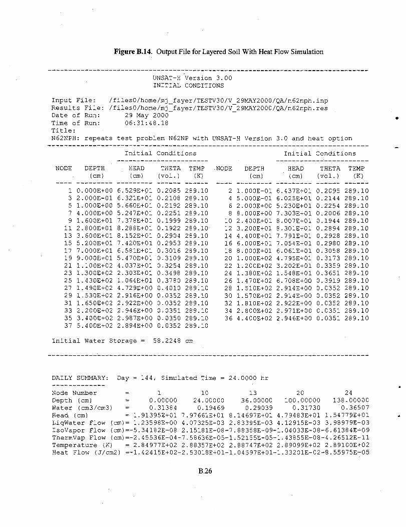
Figure B.14. Output File for Layered Soil With Heat Flow Simulation

UNSAT-H Version 3.00INITIAL CONDITIONS

/files0/home/mj_fayer/TESTV30/V_2 9MAY2000/QA/n62nph.inp/files0/home/mj_fayer/TESTV30/V_2 9MAY2000/QA/n62nph.res

29 May 200006:31:48.18

Input File:Results File:Date of Run:Time of Run:Title:N62NPH: repeats test problem N62NP with UNSAT-H Version 3.0 and heat option

NODE

13579

1113151719212325272931333537

DEPTH(cm)

O.OOOE+002.000E-011.000E+004.000E+001.600E+012.800E+013.600E+015.200E+017.000E+019.000E+011.100E+021.300E+021.430E+021.490E+021.530E+021.650E+022.200E+023.400E+025.400E+02

Initial

HEAD(cm)

6.529E+016.321E+015.660E+015.247E+017.378E+018.288E+018.152E+017.420E+016.581E+015.470E+014.037E+012.303E+011.064E+014.729E+002.916E+002.922E+002.946E+002.987E+002.894E+00

Conditions

THETA(vol.)

0.20850.21080.21920.22510.19990.19220.29040.29530.30160.31090.32540.34980.37800.40100.03520.03520.03510.03.500.0352

TEMP(K)

289.10289.10289.1028 9,10289.10289.10289.10289.10289.10289.10289.10289.10289.10289.10289.1028.9.10289.10289.10289.10

NODE

2468

1012141618202224262830323436

DEPTH(cm)

1.000E-015.000E-012.000E+008.000E+002.400E+013.200E+014.400E+016.000E+018.000E+011.000E+021.200E+021.380E+021.470E+021.510E+021.570E+021.810E+022.800E+024.400E+02

Initial

HEAD(cm)

6.437E+016.025E+015.230E+017.303E+018.007E+018.301E+017.791E+017.054E+016.061E+014.795E+013.202E+011.548E+016.708E+002.914E+002.914E+002.922E+002.971E+002.946E+00

Conditions

THETA(vol.)

0.20950.21440.22540.20060.19440.28940.29280.29800.30580.31730.33590.36510.39190.03520.03520.03520.03510.0351

TEMP(K)

289.10289.10289.10289.10289.10289.10289.10289.10289.10289.10289.10289.10289.10289.10289.10289.10289.10289.10

Initial Water Storage = 58.2248 cm

DAILY SUMMARY: Day = 144, Simulated Time = 24.0000 hr

Node Number =Depth (cm) =Water (cm3/cm3) =Head (cm) =LiqWater Flow (cm)=IsoVapor Flow (cm)=-ThermVap Flow (cm)=-Temperature (K) =Heat Flow (J/cm2) =-

0.000000.31384

1.91395E+011.23598E+005.34182E-082.45536E-042.84977E+021.42415E+02

1024.000000.19469

7.97661E+01 8.4.07325E-03 2.2.15181E-08-7.-7.58636E-05-1.2.88357E+02 2.

-2.53018E+01-1.

1336.000000.29039

14697E+0183395E-0388358E-09-52155E-05-88747E+0204597E+01-

20100.00000

0.317304.79483E+014.12915E-03•1.04033E-08•1.43855E-082.89099E+02•1.33201E-02

24138.000000.36507

1.54779E+013.98979E-03-6.61384E-09-4.26512E-112.89100E+02

-8.55975E-05

B.26

LIQUIDPRESTOR INFIL RUNOFF EVAPO TRANS DRAIN58.2248+ 1.2954+ 0.0000 - 0.0544- 0.0000- 0.0041

NEWSTOR STORAGE59.4617 vs. 59.4617

Mass Balance = 5.3876E-05 cm; Time step attempts = 1076 and.successes = 1076Daily meteorological parameters

TMAX (K) = 2.8538E+02 TMIN (K) = 2.8260E+02 VD_A (g/cm3) = 9.1063E-06WIND (m/s) = 1.8327E+00 CLOUD (frac) = 1.0000E+00SR_MEAS (J/m2) = 2.7892E+06Heat flow parameters (units = J/cm2 unless noted)RN (J/m2) = 1.4994E+06 SHF (J/m2) = -1.2859E+06 SEN (J/m2) = 1.4121E+06LE (J/m2) = 1.3733E+06 QH(NPT) = O.OOOOE+00 HBE= 5.4594E-02

DAILY SUMMARY: Day = 146, Simulated Time = 24.0000 hr

Node NumberDepth (cm)Water (cm3/cm3)Head (cm)LiqWater Flow (cm)=IsoVapor Flow (cm)=ThermVap Flow (cm)=Temperature (K) =Heat Flow (J/cm2) =

= 5

1. 0.000000.03062

90178E+056.47076E-021.78028E-011.71103E-022.92389E+027.87480E+02

1024.000000.19969

7.39746E+016.58798E-035.23987E-084.77816E-042.94276E+021.34038E+02

1336.000000.29050

8.13010E+01 4.2.96384E-03 4.

-7.83117E-09-1.9.53862E-05-1.2.91423E+02 2.6.18661E+01-1.

20100.000000.31731

79452E+0112521E-0303902E-0839025E-0689073E+0228919E+00

24138.000000.36507

1.54749E+014.00183E-036.61076E-09

15260E-072.89092E+022.31405E-01

-1

LIQUIDPRESTOR INFIL RUNOFF EVAPO TRANS DRAIN59.1813+ 0.0000+ 0.0000 - 0.2262-0.0000- 0.0041 =

NEWSTOR STORAGE58.9511 vs. 58.9514

Mass Balance = -2.7 668E-04 cm; Time step attempts = 1048 and successes = 1002Daily meteorological parameters

TMAX (K) = 2.964 9E+02 TMIN (K) = 2.8094E+02 VD_A (g/cm3) = 8.8204E-06WIND (m/s) = 8.9400E-01 CLOUD (frac) = 4.6000E-01SR_MEAS (J/m2) = 2.5806E+07Heat flow parameters (units •= J/cm2 unless noted)RN (J/m2) = 1.3859E+07 SHF (J/m2) = 3.7048E+06 SEN (J/m2) = 4.3758E+06LE (J/m2) = 5.7783E+06 QH(NPT) = O.OOOOE+00 HBE = 1.3849E+00

UNSAT-H Version 3.00SIMULATION SUMMARY

Title:N62NPH: repeats test problem N62NP with UNSAT-H Version 3.0 and heat option

Transpiration Scheme is:Potential EvapotranspirationPotential TranspirationActual TranspirationPotential Evaporation

00.0000E+000.0000E+000.0000E+000.0000E+00

[cm][cm][cm][cm]

B.27

Actual Evaporation =Evaporation during Growth =Total RunoffTotal Infiltration =Total Basal Liquid Flux (drainage) ='Total Basal Vapor Flux (temp-grad) =Total Applied Water =Actual Rainfall =.Actual Irrigation =Total Final Moisture Storage =Mass Balance Error =Total Successful Time Steps =Total Attempted Time StepsTotal Time Step Reductions (DHMAX) =Total Changes in Surface Boundary =Total Time Actually Simulated =Total Net Radiation =Total Soil-Surface Heat FlowTotal Sensible Heat Flow =Total Bottom Heat Flow =Total Latent Heat FlowHeat Balance Error =Total Convected Heat in Infilt.Total Convected Heat in Drainage =

5.5697E-01O.OOOOE+000.0000E+001.2954E+001.2205E-02O.OOOOE+001.2954E+001.2954E+00O.OOOOE+005.8951E+01-3.4355E-04

30523110

00

3.0000E+002.8188E+075.2981E+068.7065E+06O.OOOOE+001.4184E+071.8474E+005.8938E+058.1320E+03

[cm][cm][cm][cm][cm][cm][cm][cm][cm][cm][cm]

[days][J/m2][J/m2][J/m2][J/m2][J/m2][J/m2][J/m2][J/m2]

Total liquid water flow (cm) across different depths at the end of 3.0000E+00 days:

DEPTH FLOW DEPTH FLOW DEPTH FLOW

0.0000.3503.00020.00034.00056.00085.000115.000140.500150.000161.000250.000490.000

. 7.3843E-018.7273E-018.1381E-014.6612E-029.5042E-031.0193E-021.2347E-021.2272E-021.1988E-021.1852E-021.1773E-021.0905E-021.1616E-02

0.0500.7506.000

26.00040.00065.00095.000125.000145.000152.000173.000310.000540.000

9.9862E-018.0589E-017.3679E-011.5289E-028.6928E-031.1241E-021.2436E-021.2155E-021.1933E-021.1839E-021.1680E-021.0461E-021.2205E-02

0.1501.50012.00030.00048.00075.000105.000134.000148.000155.000200.500390.000

8.8570E-018.1646E-013.2415E-011.0824E-029.1992E-031.1991E-021.2382E-021.2058E-021.1888E-021.1817E-021.1427E-021.0660E-02

Total heat flow (J/cm2) across different depths:

DEPTH FLOW DEPTH FLOW DEPTH FLOW

0.0000.3503.000

5.2981E+027.3636E+025.1527E+02

006

.050

.750

.000

154

•1797E+03.4 680E+02.6650E+02

01

12

.150

.500

.000

8.5.3.

5868E+023683E+024985E+02

B.28

20.00034.00056.00085.000

115.000140.500150.000161.000250.0004 90.000

2.1722E+028.2742E+017.6030E+00-3.0946E+00-1.2170E+00-2.6016E-01 '-7.9883E-02-3.5830E-02-5.6481E-054.4605E-07

26.00040.00065.00095.000 -

125.000145.000152.000173.000310.000540.000

1.4928E+024.6713E+013.1719E-01

-2.6186E+00-7.1990E-01-1.6923E-01-6.8137E-02-1.4224E-021.2575E-06O.00OOE+O0

30.00048.00075.000105.000134.000148.000155.000200.500390.000

1.1441E+022.0871E+01-2.5866E+00-1.8836E+00-4.1752E-01-1.1498E-01-5.5323E-02-1.5446E-031.3844E-06

B.29

Figure B.15. Input File for Transpiration Simulation

r h o l y p l 4 . i n p :1 , 1 ,3 6 5 , 1 , 3 6 5 ,1 , 1 , 0 , 0 , 1 ,0 , 2 4 . 0 ,0 , 2 , 1 , 1 .0E-4 ,1 . 0 , 1 . O E - 0 5 , 1 . 0 ,2 . 0 , 1 . O E - 0 5 , 0 . 0 , 0 . 0 , 0 . 0 ,3 , 3 , 0 . 5 ,0 , 1 , 2 , 4 ,0 . 0 , 1 . O E + 0 6 , 0 , 0 . 9 9 ,0 , 0 , 0 , .0 , 0 ,0 , 0 , 0 , 0 , 0 , •0 ,0 ,0 ,0 , 0 , 0 , 0 ,0 , 0 . 0 , 0 . 01 , 0 . 6 6 , 2 8 8 . 4 6 ,1 ,43 ,1,1,1,

1 ,

1,1,1,1,1,

0 . 0 0 0 ,0 . 4 8 0 , 1 ,1 . 6 8 0 , 1 ,6 . 2 5 0 , 1 ,

2 5 . 0 0 0 , 1 ,

test case with plantsIPLANT,NGRAVIFDEND,IDTBEG,IDTENDIYS,NYEARS,ISTEAD,IFLIST,NFLISTNPRINT,STOPHRISMETH,INMAX,ISWDIF,DMAXBADELMAX, DELMIN,OUTTIMRFACT, RAINIF,DHTOL,DHMAX,DHFACTKOPT,KEST,WTFITOPBC, IEVOPT,.NFHOUR, LOWERHIRRI, HDRY,HTOP,RHAIETOPT, ICLOUD,ISHOPTIRAIN,HPRIHYS,AIRTOL,HYSTOL,HYSMXH,HYFILEiHEAT,iCONVH,DMAXHEUPPERH, TSMEAN,TSAMP,QHCTOPLOWERH, QHLEAK,TGRADIVAPOR, TORT,TSOIL,VAPDIFMATN,NPT

0 . 3 4 0 ,1 .180 ,4 . 7 5 0 ,

1 7 . 0 0 0 ,6 5 . 0 0 0 ,

0.24,

0.100,1,0

0.220,1,0.840,1,3.760,1,12.000,1,50.000,1,

6 6 0 , 1 ,2 . 4 8 0 , 1 ,8 . 5 0 0 , 1 ,

3 7 . 0 0 0 , 1 ,8 0 . 0 0 0 , 1 , 1 0 0 . 0 0 0 , 1 , 1 3 0 . 0 0 0 , 1 , 1 7 0 . 0 0 0 ,

2 2 0 . 0 0 0 , 1 , 2 7 0 . 0 0 0 , 1 , 3 3 0 . 0 0 0 , 1 , 3 9 0 . 0 0 0 ,5 3 3 . 0 0 0 , 1 , 6 8 6 . 0 0 0 , 1 , 8 3 8 . 0 0 0 , 1 , 9 9 1 . 0 0 0 ,

1 , 1 1 4 3 . 0 0 0 , 1 , 1 2 9 5 . 0 0 0 , 1 , 1 4 4 8 . 0 0 0 , 1 , 1 5 8 0 . 0 0 01 , 1 6 4 9 . 0 0 0 , 1 , 1 7 0 9 . 0 0 0 , 1 , 1 7 4 4 . 0 0 0 , 1 , 1 7 7 9 . 0 0 0 ,1 , 1 8 0 3 . 0 0 0 , 1 , 1 8 1 9 . 0 0 0 , 1 , 1 8 2 9 . 0 0 0 ,

SOIL WATER CONTENT DATA0 . 4 1 4 2 , 0 . 0 , 2 9 . 8 , 1 . 6 3 ,

SOIL CONDUCTIVITY DATATHET,THTR,AIRINT,B

1.0,

1,1,0,944,120,4.0,

24o,

1,

0.0.1,

.8,29

329.326.325.319.302.320.692.867.

1087.1312.1187.1,121

0,182034,1

1

.8,1.^

025,4 62,439,901,286,144,252,077,887,374,037,,273,

,1.03.0,

63,2.0, RKMOD,SK,AIRINT

327.940,326.317,324.400,317.326,297.413,352.646,811.017,908.831,

1274.681,1269.146,1171.491,

LEAF,NFROOT,

,243,1.03,274,0.

1, 1, 1,

NDAY327.156326.228322.842313.506297.955425.380841.007968.274

1388.4941240.5551161.566

NUPTAK,NFPETBARENDLAI

. 0, IDLAI,AA,B1,

1, 1,

,B,EPIT

326.721,325.997,321.662,308.565,305.454,533.201,845.091,1010.295,1352.624,1209.547,

f

,NSOW,NHRVST

VLAI pairsB2

1, 1, 1,

B.30

2,2 5 ,

365,365,

2,3 1 ,

365,365,

2,40,

365,365,

3 ,53 ,

365,

4,74,

365,

5,105,365,

2.040E+03,1.500E+03,3.000E+01-0.21,0.7,0.5,0.1,2.7,0.0600,0.0822,0.0580,0.0162,00.0138,0.0267,0.0202,0.0221,00.1133,0.1462,0.2107,0.1741,0< similar lines deleted >0.1810,0.0727,0.0683,0.1199,00.064 6,0.1207,0.2058,0.1956,00.1528,0.1193,0.1012,0". 1334,0

63, NWATER2, 1, 4,1.000,4.0, 0.1524,

10.0, 0.0000,13.0, 0.0254,14.0, 0.0000,7, 1, 2,1.000,

10.0, 0.0254,11.0, 0.0000,

< similar lines deleted >359, 1, 2,1.000,0.0, 0.0762,1.0, 0.0000,

360, 1, 6,1.000,15.0, 0.2032,19.0, 0.0000,21.0, 0.0254,22.0, 0.0000,23.0, 0.0254,24.0, 0.0000,

.0703,0

.0832,0

.1487,0

8, 11, 16, 20,365, 365, 365, 365,365, 365, 365, 365,

THETAW,THETAD,THETANPCA,PCB,PCC,PCD,PCE

.0195,0.0225,0.0206,

.3136,0.4497,0.3908,

.2446,0.1403,0.1193,

.0689,0.

.1071,0.

.0322,(Total for 1974 = 13.4620 cm)

1.0150,0.1759,0.1364,1.0648,0.0150,0.0270,

B.3I

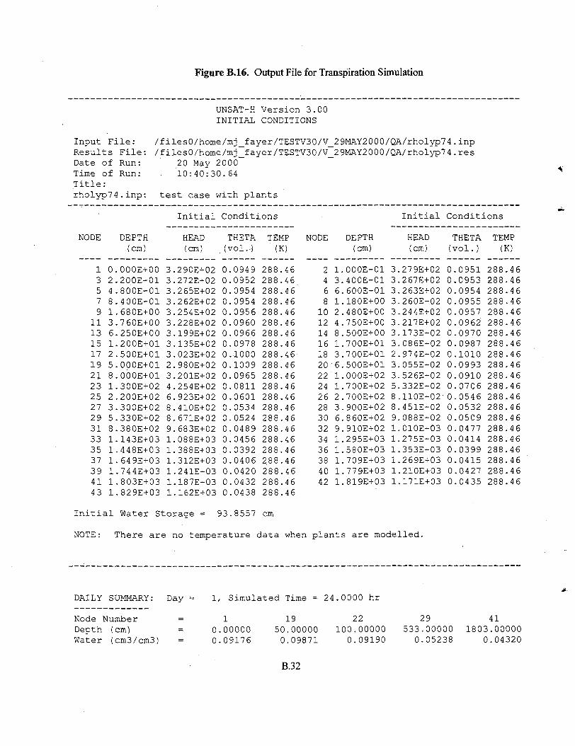
Figure B.16. Output File for Transpiration Simulation

UNSAT-H Version 3.00INITIAL CONDITIONS

Input File: /files0/home/mj fayer/TESTV30/V 2 9MAY2000/QA/rholyp74.inpResults File: /filesO/home/mj_fayer/TESTV30/V~DateTimeTitle

of Run:of Run::

rholyp7 4.inp:

NODE

13579

1113151719212325272931333537394143

DEPTH .(cm)

0.000E+002.200E-014.800E-018.400E-011.680E+003.760E+006.250E+001.200E+012.500E+015.000E+018.000E+011.300E+022.200E+023.300E+025.330E+028.380E+021.143E+031.448E+031.649E+031.744E+031.803E+031.829E+03

20 May 2000• 10:40:3C1.64

test case with plants

Initial

HEAD(cm)

3.290E+023.272E+023.265E+023.262E+023.254E+023.228E+023.199E+023.135E+023.023E+022.980E+023.201E+024.254E+026.923E+028.410E+028.671E+029.683E+021.088E+031.388E+031.312E+031.241E+031.187E+031.162E+03

Conditions

THETA(vol..)

0.09490.09520.09540.09540.09560.09600.09660.09780.10000.10090.09650.08110.06010.05340.05240.04890.0456.0.03920.04060.04200.04320.0438

TEMP(K)

288.46288.46288.46288.46288.46288.46288.46288.46288.46288.46288.46288.46288.46288.46288.46288.46288.46288.46288.46288.46288.46288.46

NODE

2468

1012141618202224262830323436384042

29MAY2000/QA/rholyp74.res

DEPTH(cm)

1.000E-013.400E-016.600E-011.180E+002.480E+004.750E+008.500E+001.700E+013.700E+016.500E+011.000E+021.700E+022.700E+023.900E+026.860E+029.910E+021.295E+031.580E+031.709E+031.779E+031.819E+03

Initial

HEAD(cm)

3.279E+023.267E+023.263E+023.260E+023.244E+023.217E+023.173E+023.086E+022.974E+023.055E+023.526E+025.332E+028.110E+02'8.451E+029.088E+021.010E+031.275E+031.353E+031.269E+031.210E+031.171E+03

Conditions

THETA(vol.)

0.09510.09530.09540.09550.09570.09620.09700.09870.10100.09930.09100.07060.05460.05320.05090.04770.04140.03990.04150.04270.0435

TEMP(K)

288.46288.46288.46288.46288.46288.46288-46288.46288.46288.46288.46288.46288.46288.46288.46288.46288.46288.46288.46288.46288.46

Initial Water Storage = 93.8557 cm

NOTE: There are no temperature data when plants are modelled.

DAILY SUMMARY: Day

Node NumberDepth (cm)Water (cm3/cm3)

1, Simulated Time = 24.0000 hr

0.000000.09176

1950.000000.09871

22100.00000

0.09190

29533.00000

0.05238

411803.00000

0.04320

B.32

Head (cm) = 3.47669E+02 3.08665E+02 3.46814E+02 8.67064E+02 1.18701E+03LiqWater Flow (cm)=-5.98420E-02 1.05816E-01 1.09368E-01 1.65334E-03 1.23728E-05IsoVapor Flow (cm)=-9.63501E-08 1.49752E-08 9.98989E-08 1.30047E-08-4.73607E-08Plant Sink (cm) = O.OOOOOE+00 0.00000E+00 O.OOOOOE+00 O.OOOOOE+00 0.00000E+00

LIQUIDPRESTOR INFIL RUNOFF EVAPO TRANS DRAIN NEWSTOR STORAGE93.8557+ 0.0000+ 0.0000 - 0.0600- 0.0000- 0.0000 = 93.7957 vs. 93.7957

Mass Balance = -4.8444E-06 cm; Time step attempts = 44 and successes = 44Evaporation: Potential = 0.0600 cm, Actual = 0.0600 cm

Transpiration: Potential = 0.0000 cm, Actual = 0.0000 cm

DAILY SUMMARY: Day = 365, Simulated Time =? 24.0000 hr

Node NumberDepth (cm)Water (cm3/cm3)Head (cm)LiqWater Flow (cm)=IsoVapor Flow (cm)=Plant Sink (cm)

= 1

0.000000.00249

.24092E+05

1950.000000.05259

. 61453E+02•6.30966E-07 2.21941E-03•2.56204E-02 2.55336E-08-O.OOOOOE+00 0.00000E+00

22100.000000.05042

9.22571E+027.47966E-04•1.63827E-080.00000E+00

29533.000000.05655

7.65280E+022.99631E-033.07510E-08-O.0O00OE+OO

411803.00000

0.043431.17675E+031.18877E-054.74292E-080.00000E+00

LIQUIDPRESTOR INFIL RUNOFF EVAPO TRANS DRAIN NEWSTOR STORAGE88.8665+ 0.0000+ 0.0000 - 0.0255- 0.0000- 0.0000 = 88.8410 vs. 88.8416

Mass Balance =Evaporation:

Transpiration:

-5.9697E-04 cm; Time step attempts = 55 and successesPotential = 0.0322 cm, Actual = 0.0255 cmPotential = 0.0000 cm, Actual = 0.0000 cm

42

UNSAT-H Version 3.00SIMULATION SUMMARY

Title:rholyp7 4.inp: test case with plants

Transpiration Scheme is:Potential EvapotranspirationPotential TranspirationActual TranspirationPotential EvaporationActual EvaporationEvaporation during GrowthTotal Runoff•Total InfiltrationTotal Basal Liquid Flux (drainage)Total Basal Vapor Flux (temp-grad)

1.7494E+022.7426E+002.4068E+001.7220E+021.6042E+013.7537E+000.0000E+001.3462E+010.0000E+00O.OOOOE+00

[cm][cm][cm][cm][cm][cm][cm][cm][cm][cm]

B.33

Total Applied WaterActual Rainfall =Actual Irrigation =Total Final Moisture StorageMass Balance Error =Total Successful Time StepsTotal Attempted Time StepsTotal Time Step Reductions (DHMAX) =Total Changes in Surface Boundary =Total Time Actually Simulated =

1.3462E+011.34 62E+010.0000E+008.8842E+012.7345E-02

1834422984

08555

3.6500E+02

[cm][cm]

• [cm]

[cm][cm]

[da's

Total liquid water flow (cm) across different depths at the end of 3.6500E+02 days:

DEPTH FLOW DEPTH FLOW DEPTH FLOW

0.0000.2800.7502.0805.500

14.50043.50090.000

.195.000360.000762.000

1219.0001614.5001761.5001824.000

-2.5800E+004.5.134E+001.4356E+00

-1.2040E+D0 '-1.9634E+00-1.9259E+00-1.0462E+006.1801E-012.7586E+002.0658E+005.7145E-013.4906E-014.6511E-021.5488E-021.2199E-03

0.0500.4101.0103.1207.375

21.00057.500

115.000245.000461.500914.500

1371.5001679.0001791.0001829.000

7.3153E+003.5521E+006.6549E-01

-1.6475E+00-2.0265E+00-1.7409E+00-5.5352E-011.4307E+002.7389E+001.4292E+004.3253E-011.9109E-013.2576E-028.9277E-030.0000E+00

0.1600.5701.4304.255

10.25031.00072.500150.000300.000609.500

1067.0001514.0001726.5001811.000

5.8761E+002.4286E+00

-2.4081E-01-1.8736E+00-2.0644E+00-1.4527E+00-8.2349E-032.2454E+002.3880E+008.1194E-013.8474E-017.8259E-022.2887E-024.3016E-03

Total plant water uptake (cm) at different depths:

DEPTH WATER UPTAKE DEPTH WATER UPTAKE DEPTH WATER UPTAKE

0.0000.3400.8402.4806.250

17.00050.000100.000220.000390.000838.0001295.0001649.0001779.0001829.000

O.OOOOE+009.4469E-053.0951E-043.0899E-031.9701E-021.3950E-011.8325E-012.0078E-012.5893E-01O.OOOOE+000.0000E+000.0000E+00O.OOOOE+00O.OOOOE+000.0OOOE+00

0.1000.4801.1803.7608.500

25.00065.000130.000270.000533.000991.0001448.0001709.0001803.000

6.6593E-051.3563E-046.1783E-045.7 97 6E-034.'1294E-022.0286E-011.6005E-012.4697E-012.0472E-010.0000E+000.0000E+000.0000E+000.0000E+000.0000E+00

0.2200.6601.6804.750

12.00037.00080.000170.000330.000686.000

1143.0001580.0001744.0001819.000

7.7425E-051.8635E-041.2850E-039.1241E-037.9159E-022.0379E-011.6120E-012.8381E-010.0000E+000.0000E+00O.OOOOE+000.0000E+000.0000E+000.0000E+00

B.34

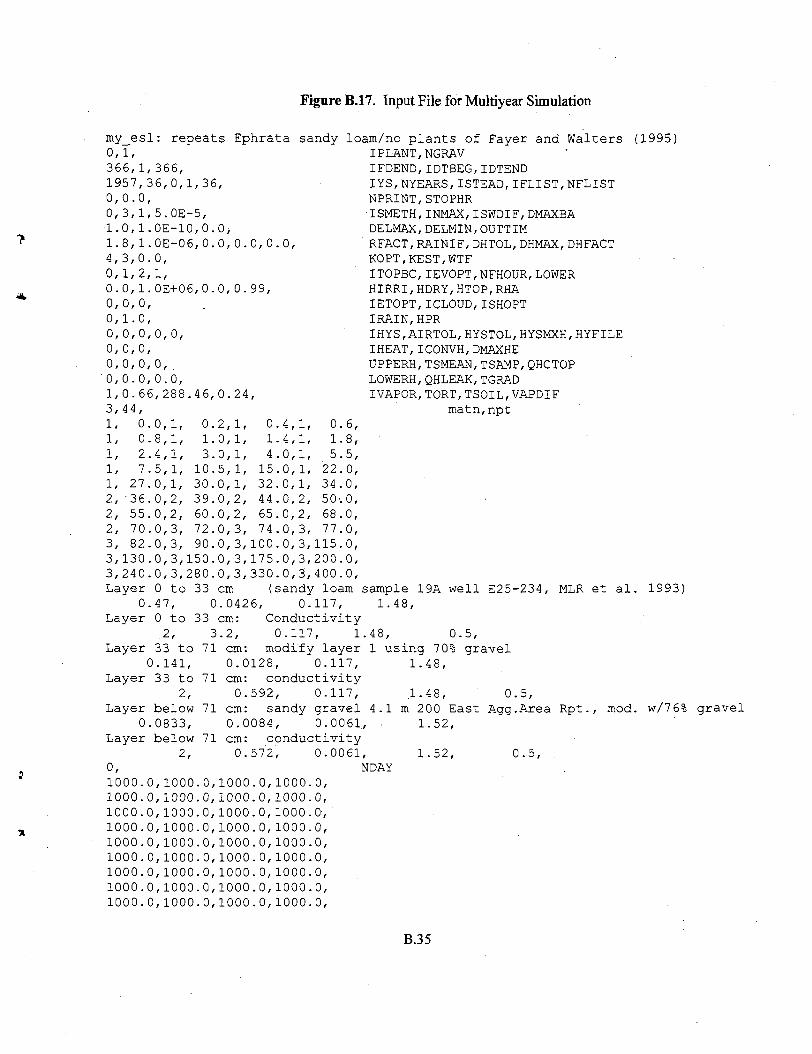
Figure B.17. Input File for Multiyear Simulation

my_esl: repeats Ephrata sandy loam/no plants of Fayer and Walters (1995)0,1,366,1,366,1957,36,0,1,36,0,0.0,0,3,1,5.OE-5,1.0,1.0E-10,0.0,1.8,1.0E-06,0.0,0.0,0.0,4,3,0.0,0,1,2,1,0.0,1.0E+06,0.0,0.99,0,0,0,0,1.0,0,0,0,0,0,0,0,0,0,0,0,0,0,0.0,0.0,1,0.66,288.46,0.24,

44,3,1,1,1,1,1,2,2,2,3,

1,1,

0.0,0.8,2.4,1,7.5,1,

27.0,1,36.0,2,

.0,2,

2,1,0,1,

55.70.82.

0,3,0,3,

3.0,1,10.5,1,30.0,1,39.0,2,60.0,2,72.0,3,

0.1.4.

15.32.44.65.74.

4,1,4,1,0,1,0,1,0,1,0,2,0,2,0,3,

0.1.5.

22.34.

6,8,5,0,0,

IPLANT,NGRAVIFDEND,IDTBEG,IDTENDIYS,NYEARS,ISTEAD,IFLIST,NFLISTNPRINT,STOPHRISMETH,INMAX,ISWDIF,DMAXBADELMAX,DELMIN,OUTTIMRFACT,RAINIF,DHTOL,DHMAX,DHFACTKOPT,KEST,WTFITOPBC,IEVOPT,NFHOUR,LOWERHIRRI,HDRY,HTOP,RHAIETOPT,ICLOUD,ISHOPTIRAIN,HPRIHYS,AIRTOL,HYSTOL,HYSMXH,HYFILEIHEAT,ICONVH,DMAXHEUPPERH,TSMEAN,TSAMP, QHCTOPLOWERH,QHLEAK,TGRADIVAPOR,TORT,TSOIL,VAPDIF

matn,npt

50-. 0,68.0,77.

90.0,3,100.0,3,1150,0,

3,130.0,3,150.0,3,175.0,3,200.0,3,240.0,3,280.0,3,330.0,3,4 00.0,Layer

0Layer

0 to 33 cm (sandy loam sample 19A well E25-234, MLR et al. 1993)1.48,,47, 0.0426, 0.117,

0 to 33 cm: Conductivity2, 3.2, 0.117, 1.48, 0.5,

Layer 33 to 71 cm: modify layer 1 using 70% gravel0.141,

Layer 33 to 712,

0.0128, 0.117, 1.48,cm: conductivity0.592, 0.117, .1.48, 0.5,

NDAY

Layer below 71 cm: sandy gravel 4 . 1 m 200 East Agg.Area Rpt., mod. w/76% gravel0.0833, 0.0084, 0.0061, . 1.52,

Layer below 71 cm: conductivity2, 0.572, 0.0061, 1.52, 0.5,

0,1000.0,1000.0,1000.0,1000.0,1000.0,1000.0,1000.0,1000.0,1000.0,1000.0,1000.0,1000.0,1000.0,1000.0,1000.0,1000.0,1000.0,1000.0,1000.0,1000.0,1000.0,1000.0,1000.0,1000.0,1000.0,1000.0,1000.0,1000.0,1000.0,1000.0,1000.0,1000.0,1000.0,1000.0,1000.0,1000.0,

B.35

1000.0,1000.0,1000.0,1000.0,1000.0,1000.0,1000.0,1000.0,~/hms/dayv30/petpen_u7~/hms/dayv30/raindat

B.36

Figure B.18. Output File for Multiyear Simulation

UNSAT-H Version 3.00INITIAL CONDITIONS

Input File: /filesO/home/mj_fayer/TESTV30/V_29MAY2000/QA/my_esl.inpResults File: /files0/home/mj_fayer/TESTV30/V_29MAY2000/QA/my_esll957.resDate of Run: 20 May 2000Time of Run: 11:39:59.84Title:my_esl: repeats Ephrata sandy loam/no plants of Fayer and Walters (1995)

NODE

135791113151719212325272931333537394143

DEPTH(cm)

0.000E+004.000E-018.000E-011.400E+002.400E+004.000E+007.500E+001.500E+012.700E+013.200E+013.600E+014.400E+015.500E+016.500E+017.000E+017.400E+018.200E+011.000E+021.300E+021.750E+022.400E+023.300E+02

Initial

HEAD(cm)

1.000E+031.000E+031.000E+031.000E+031.000E+031.000E+031.000E+031.000E+031.000E+031.000E+031.000E+031.000E+031.000E+031.000E+031.000E+031.000E+031.000E+031.000E+031.000E+031.000E+031.000E+031.000E+03

Conditions

THETA(vol.)

0.08600.08600.08600.08600.08600.08600.08600.08600.08600.08600.02580.02580.02580.02580.02580.03700.03700.03700.03700.03700.03700.0370

TEMP

(K)

288.46288.46288.46288.46288.46288.46288.46288.46288.46288.46288.46288.46288.46288.46288.46288.46288.46288.46288.46288.46288.46288.46

NODE

2468

1012141618

. 20222426283032343638404244

DEPTH(cm)

2.000E-016.000E-011.000E+001.800E+003.000E+005. 500E+001.050E+012.200E+013.000E+013.400E+013.900E+015.000E+016.000E+016.800E+017.200E+017.700E+019.000E+011.150E+021.500E+022.000E+022.800E+024.000E+02

Initial

HEAD(cm)

1.000E+031.000E+031.000E+031.000E+031.000E+031.000E+031.000E+031.000E+031.000E+031.000E+031.000E+031.000E+031.000E+031.000E+031.000E+031.000E+031.000E+031.000E+031.000E+031.000E+031.000E+031.000E+03

Conditions

THETA(vol.)

0.08600.08600.08600.08600.08600.08600.08600.08600.08600.08600.02580.02580.02580.02580.03700.03700.03700.03700.03700.03700.03700.0370

TEMP(K)

288.46288.46288.46288.46288.46288.46288.46288.46288.46288.46288.46288.46288.46288.46288.46288.46288.46288.46288.46288.46288.46288.46

I n i t i a l Water Storage = 16.1265 cm

DAILY SUMMARY: Day = 1, Simulated Time = 24.0000 hr

Node NumberDepth (cm)Water (cm3/cm3)Head (cm)

1830.000000.08605

2660.000000.02583

3490.000000.03696

38150.00000

0.03703

41240.00000

0.037031.00000E+03 1.00000E+03 1.00501E+03 1.00001E+03 1.00000E+03

LiqWater Flow (cm)= 1.94331E-06 3.59533E-07 3.23057E-03 3.74461E-03 3.74488E-03IsoVapor Flow (cm)=-2.60821E-12 6.91520E-14-8.15460E-10-4.13565E-13-1.10499E-17

B.37

LIQUIDPRESTOR INFIL RUNOFF EVAPO TRANS DRAIN16.1265+ 0.0762+ 0.0000 - 0.0074- 0.0000- 0.0037

NEWSTOR STORAGE16.1916 vs. 16.1912

Mass Balance = 4.3197E-04 cm; Time step attempts = 182 and successes = 158Evaporation: Potential = 0.0078 cm, Actual = 0.0074 cm

DAILY SUMMARY: Day = 365, Simulated Time = 24.0000 hr

Node NumberDepth (cm)Water (cm3/cm3)Head (cm)

300

18.00000.20033

600

26.00000.04368

900

34.00000.03305

1500

38.ooooo •.03351

2400

41.00000.03402

= 6.60400E+01 1.64524E+02 1.35328E+03 1.30476E+03 1.-25271E+03LiqWater Flow (cm)= 1.99832E-03 1.17176E-03 1.52970E-04 5.36961E-04 1.12617E-03IsoVapor Flow (cm)=-2.91168E-08 1.54275E-06-5.89892E-09-4.39429E-09-2.56746E-09

LIQUIDPRESTOR INFIL RUNOFF EVAPO TRANS DPAIN19.1024+ 0.0000+ 0.0000 - 0.0204- 0.0000- 0.0020 =

NEWSTOR19.0800 vs.

STORAGE19.0800

Mass Balance = -7.2170E-05 cm; Time step attempts = 26 and successes = 25Evaporation: Potential = 0.0538 cm, Actual = 0.0204 cm

UNSAT-H Version 3.00SIMULATION SUMMARY

Title:my_esl: repeats Ephrata sandy loam/no plants of Fayer and Walters (1995)

Transpiration Scheme is:Potential EvapotranspirationPotential TranspirationActual TranspirationPotential EvaporationActual EvaporationEvaporation during GrowthTotal RunoffTotal InfiltrationTotal Basal Liquid Flux (drainage)Total Basal Vapor Flux (temp-grad)Total Applied WaterActual RainfallActual IrrigationTotal Final Moisture StorageMass Balance ErrorTotal Successful Time StepsTotal Attempted Time Steps

1.6642E+020.0000E+000.0000E+001.6642E+021.6833E+010.0000E+002.9421E-012.0762E+011.0467E+000.0000E+002.1057E+012.1057E+010.0000E+001.9080E+01

-7.0611E-022396832145

[cm][cm][cm][cm][cm][cm][cm][cm][cm][cm][cm][cm][cm][cm][cm]

B.38

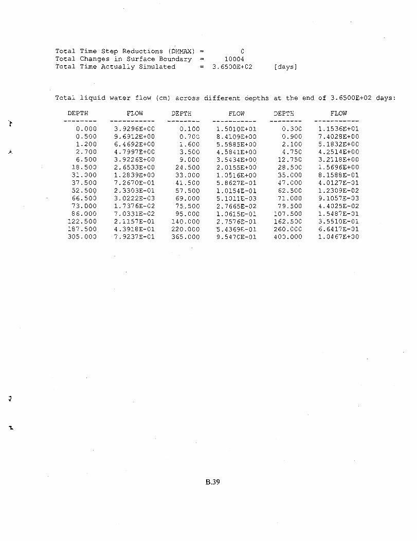
Total Time Step Reductions (DHMAX) = 0Total Changes in Surface Boundary = 10004Total Time Actually Simulated = 3.6500E+02 [days]

Total liquid water flow (cm) across different depths at the end of 3.6500E+02 days:

DEPTH FLOW DEPTH FLOW DEPTH FLOW

0.0000.5001.2002.7006.500

18.50031.00037.50052.50066.50073.00086.000122.500187.500305.000

3.9296E+009.6912E+006.4 692E+004.7997E+003.9226E+002.6533E+001.2839E+007.2670E-012.3303E-013.0222E-031.7376E-027.0331E-022.1157E-014.3918E-017.9237E-01

0.1000.7001.6003.5009.000

24.50033.00041.50057.50069.00075..50095.000140.000220.000365.000

1.5010E+018.4109E+005.5885E+004.5841E+003.5434E+002.0155E+001.0516E+005.8627E-011.0154E-015.1011E-032.7665E-021.0615E-012.7576E-01"5.4369E-019.5470E-01

0.3000.9002.1004.750

12.75028.50035.00047.00062.50071.00079.500

107.500162.500260.000400.000

1.1536E+017.4028E+005.1832E+004.2514E+003.2118E+001.5696E+008.1588E-014.0127E-011.2309E-029.1057E-034.4025E-021.5487E-013.5510E-016.6417E-011.0467E+00

B.39

PNNL-13249

Distribution

No. ofCopies

OFFSITE

B AlbrightDesert Research Institute2215 Raggio ParkwayReno,NV 89512

B AndraskiUSGS333 West Nye LaneCarson City, NV 89706

MAnkenyD.B. Stephens and Associates6020 Academy NESuite 100Albuquerque, NM 87109

C BensonUniv. of Wisconsin-Madison2214 Engineering Hall1415 Engineering DriveMadison, WI 53706

B. ScanlonBureau of Economic GeologyUniversity of Texas at AustinUniversity StationBoxXAustin, TX 78713

M YoungDesert Research Institute755 Flamingo RoadLas Vegas, NV 89119

ONSITE

3 Fluor Federal Services

RKhaleelFMMannRJPuigh

Pacific Northwest National

CRColeJL DownsMJFayer(20)GWGeeLH GerhardsteinCT KincaidRRKirkhamRJ LenhardPD MeyerGP StreileJK TarantinoALWardInformation Release (7)

B4-43HO-22B4-43

Laboratory

K9-36K6-85K9-33K9-33K7-28K9-33K9-33K9-33

BPOK9-33K9-41K9-33

Distr.l