Unlocking the Phase Lock Loop - Part 2biitcomm/research/references/Other... · Unlocking the Phase Lock Loop - Part 2 2 intuitively see that if a transient is large, the system will

Unlocking the Phase Lock Loop - Part 2

www.complextoreal.com

1

Intuitive Guide to Principles of Communications www.complextoreal.com

Unlocking the Phase Lock Loop - Part 2 Tracking and Acquisition behavior A PLL produces a carrier that synchronizes in phase and frequency with an independent external signal. The PLL controls the phase of its internal signal such that the error - the difference between its phase and that of the input signal - is kept at a minimum while the frequency of its signal is kept the same as the input signal. PLL does this by continuously adjusting its frequency although what we track is phase. In Part I we looked at how the PLL using just three functional blocks, a phase detector, a low pass filter and a VCO accomplishes this. A PLL has two main behavior modes; Tracking Mode - The PLL is already locked on to the signal. What the PLL does to keep itself aligned with the incoming signal in light of frequency and phase disturbances, is called Tracking. This behavior is analyzed assuming linear behavior. Acquisition Mode � The PLL is either out of lock or is just starting up to lock on to a signal. This mode is non-linear, difficult to analyze and understand. Tracking Tracking assumes that PLL has already acquired the signal and is now trying to keep up with it. It is kind of like what a bicycle rider does to stay on the bike. The tracking behavior has a steady-state and a transient mode of response. When PLL is locked up and nothing is changing, the PLL shows a steady state behavior. When things are changing, we see transient behavior. Transients also occur at acquisition and occur again as soon as there is a change in the incoming signals frequency or phase. However as long as the changes are small, the PLL recovers from these disturbances and gets back to steady state. For example, take the bicycle rider who runs into a little bump in the road, the bicycle lurches to the side but the rider recovers (does not fall down) and gets back to his steady speed. This immediate response to a changed condition comes under the tracking mode. Whereas getting on the bike and starting up would be considered an acquisition mode. During the transient, whether during acquisition or tracking, the error signal generated by the PLL oscillates in response to large differences between the VCO and the incoming signal phase. (Its always phase!) The transient part is very important because we can



2

intuitively see that if a transient is large, the system will be unable to return to steady state and the PLL will lose lock. How a PLL behaves during the transient phase of tracking is a function of the loop natural frequency, its damping factor and the loop gains. The phase error signal transfer equation of a 2nd order PLL was developed in Part I, (Eq. 16) and is given by

( )( )

( )i

ev d

s ss

s K K F sθθ =

+ (1)

Here )(seθ is the error produced by the PLL, the ( )i sθ is the phase of the input signal. Kv is the gain of the VCO, Kd the gain of the phase detector and F(s) the transfer function of the filter and may include a gain. You recall that the error signal is a measure of phase difference between the input signal and the VCO signal. We will see how this error signal changes when it is subjected to disturbances. I wanted very much to explain the behavior of PLL without ever referring to the Laplace transform, but as much as I would like, this just cannot be done. In Part I, I gave some important Laplace relationships that are needed for understanding the PLL. Here is one more property that we need to explain the transient behavior. This property is called the Final Value Theorem and goes like this,

)(lim)(lim0

sstst

θθ→∞→

= (2)

It states that to find the steady-state behavior of a signal, we take the limit of s times its Laplace Transform. This relationship helps us determine the steady state response of a system. Quite a few things can wrong for a PLL that is already in lock. We can classify these disturbances in four broad categories. 1. There is a sudden phase shift at the input. 2. The input frequency does a jump. 3. The input frequency begins to change slowly such as due to Doppler. 4. There is noise at the input or inside the PLL.



3

Case 1: There is a sudden phase change at the input. What happens to the steady state error in response to a phase step and how does the PLL which was locked react to this? How big of phase step can a PLL recover from? We will now answer these questions. The change in the phase of the incoming signal is represented as a

( ) ( )i t u tθ θ= ∆ (3) u(t) is the unit step function and θ∆ is the size of the phase change. The instantaneous phase has just done a jump from its old value to a new value by θ∆ . The Laplace transform of a unit step function with a phase change of θ∆ is

( )i ss

θθ ∆= (4)

This is Laplace transform of the phase step equation (3). Apply this value of ( )i sθ to (1), multiply it by s and then take limit per Final Value Theorem of Eq. 2, we get

2

0lim ( ) lim

(0

)et so d

sts K K F s s

θθ→∞ →

∆=+

= (5)

Setting s = 0 in this limit, the expression evaluates to 0. This says that the error signal in time will go to zero in response to a phase step at the input. (assuming that F(s) is not = 0 which is not possible anyway.) In other words, no matter, how big the phase step, the loop will eventually track it out and there will be no remaining steady-state error from a phase step. Imagine a swing, no matter high we pull the swing to start it; it will eventually come to rest. Same situation here. The loop tracks out the initial phase push. Theoretically speaking a PLL can recover from any phase step but we don�t mean any phase step, it is limited generally to 180o or less as is obvious from the swing problem. But we can actually recover from phases larger than 180o because mathematically the swing would then flip over the top and once again will return to steady state. Second question is; how long will it take the loop to track out this phase error? This is an important question and helps determine what the loop parameters need to be so that tracking time is not excessive and most importantly is within a bit or two of the signal symbol rate.



4

The equation that describes this behavior is given below (From Reference 1, 2 and 3.) It is developed by substituting the filter parameters in (1) and then applying the Final value Theorem. (You will not find this equation explicitly derived in any of the PLL books. Most books just tabulate these equations, including books by Gardener and Best.)

2 2

2( ) cos 1 sin 1

1nt

e n nt t t e ζωζθ θ ζ ω ζ ωζ

− = ∆ − − − −

(6)

(valid for ζ < 1) A little bit about the damping factor, ζ. The larger the damping factor the looser the system and more violent the oscillations. (Most PLL use a damping factor of .707, which is about optimum for signal processing applications.) Figures 1 shows how the loop behaves in time domain to a phase step error.

-0.6

-0.4

-0.2

0

0.2

0.4

0.6

0.8

1

1.2

0 2 4 6 8 10 12

wn t

Erro

r/pha

se s

tep

zeta = .3 zeta = .5 zeta = .707 zeta = .9

Figure 1 � Normalized transient response to a phase step In this graph both the x and the y axis have been normalized. The y-axis is error signal magnitude divided by the phase step. It starts at 1.0, because initially the error signal is exactly equal to the phase step. Then the error signal level begins to drop and at (wnt) > 10 it has completely tracked out the phase step and the steady state error has returned to zero. The x-axis is also normalized by the natural frequency. The time to reach steady state is inversely proportional to wn. A large wn means a small settling time, t. Now we plot the same curves but remove the normalization so we can see how the magnitude of the error signal varies as the phase step is changed.



5

-0.1

-0.05

0

0.05

0.1

0.15

0.2

0 2 4 6 8 10 12

wn t

Erro

r/pha

se s

tep

zeta = .5 zeta = .707

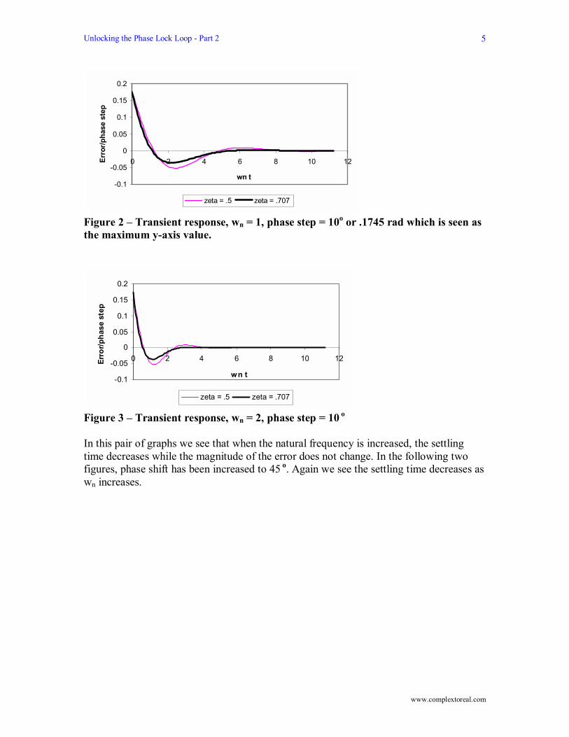
Figure 2 � Transient response, wn = 1, phase step = 10o or .1745 rad which is seen as the maximum y-axis value.

-0.1

-0.05

0

0.05

0.1

0.15

0.2

0 2 4 6 8 10 12

wn t

Erro

r/pha

se s

tep

zeta = .5 zeta = .707

Figure 3 � Transient response, wn = 2, phase step = 10 o In this pair of graphs we see that when the natural frequency is increased, the settling time decreases while the magnitude of the error does not change. In the following two figures, phase shift has been increased to 45 o. Again we see the settling time decreases as wn increases.



6

-0.4

-0.2

0

0.2

0.4

0.6

0.8

1

0 2 4 6 8 10 12

wn t

Erro

r/pha

se s

tep

zeta = .5 zeta = .707

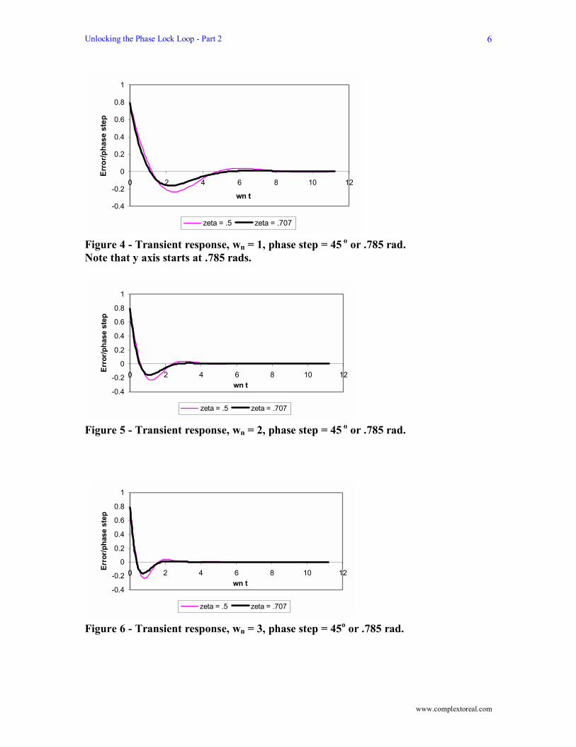
Figure 4 - Transient response, wn = 1, phase step = 45 o or .785 rad. Note that y axis starts at .785 rads.

-0.4

-0.2

0

0.2

0.4

0.6

0.8

1

0 2 4 6 8 10 12wn t

Erro

r/pha

se s

tep

zeta = .5 zeta = .707

Figure 5 - Transient response, wn = 2, phase step = 45 o or .785 rad.

-0.4

-0.2

0

0.2

0.4

0.6

0.8

1

0 2 4 6 8 10 12wn t

Erro

r/pha

se s

tep

zeta = .5 zeta = .707

Figure 6 - Transient response, wn = 3, phase step = 45o or .785 rad.



7

-1

-0.5

0

0.5

1

1.5

2

0 2 4 6 8 10 12

wn t

Erro

r/pha

se s

tep

zeta = .5 zeta = .707

Figure 7 - Transient response, wn = 3, phase step = 90o or 1.57 rad. The interesting thing about these curves is that no matter how large the phase error, it can be tracked out. Only the magnitude of the error signal changes. The tracking time does not seem to be a function of the phase step but is definitely a function of the natural frequency of the PLL. Important result: The settling time of a PLL in response to a phase step is a function of its natural frequency. A larger natural frequency gives a smaller settling time. Example: For a system with a natural frequency of 20 rad/sec, the settling time is

6 .7076 .0003 sec

20000

nt for

t

ω ζ≈ =

= =

Keep in mind that wn, the natural frequency is different from loop bandwidth by approximately a factor of two. Most PLLs are specified by a loop bandwidth in sympathy to specifying a PLL as a filter. A large natural frequency would then seem to be the ticket to a fast-reacting system. But a large natural frequency also lets in more noise. The noise degrades the performance by a different mechanism. There is balance somewhere between large and a small wn. Large wn is good for response performance and bad for noise tolerance. Case 2: The input frequency does a jump. Now let's assume that instead of phase change, the input signal does an abrupt frequency shift such that a ω∆ is presented at the input to the PLL. We can write this as the sum of the original frequency plus a step function times the frequency shift.

0( ) ( )i t u tω ω ω= + ∆ (7)



8

The frequency ωo has now changed by ∆ω . The phase change now seen by the PLL (because phase change is all a PLL is capable of experiencing, so we convert everything into phase) instead of being a step is a ramp, that is the phase changes continuously over a certain period of time t, to give us the frequency shift we specify. We define input phase as a function of time as

tti ωθ ∆=)( (8) The Laplace Transform of this function is

2( )i ss

ωθ ∆= (9)

Now apply this to PLL transfer function (1) multiply it by s and then take the limit to find the time domain response.

2

20lim ( ) l

( )

im( )

o d

et sv d

sts K K F s s

K K F s

ωθ

ω

→∞ →

∆

=

=

∆+

(10)

This is steady state error due to a frequency step. This result is different from the one we obtained for phase step in (3). First of all the steady-state error is not zero like it was for phase step. This result says that a steady state error will exist and will not be tracked out when there is a frequency change at the input to the PLL. The denominator of this equation is the gain of the loop which means we should use an active filter with a large gain and make sure that all the other components also have large gains. This will give large loop gain and better tolerance for frequency shifts.

( )O v dK K K F s=

The loop gain is equal to K0 which has dimensions of time-1 or frequency, Hz. Now we can rewrite (10) as

eOKωθ ∆= (11)

The time domain behavior for this case is given by (Ref. 1, 2)



9

tn

ne

nett ζωωζζω

ωθ −

−

−

∇= 2

21sin

1

1)( (12)

The error in this case starts at zero and begins to build up and then damps out according to the damping factor of the loop. Intuitively this is because the phase step is zero to begin with but continues building up.

-0.004

-0.002

0

0.002

0.004

0.006

0.008

0.01

0 2 4 6 8 10 12 14wn t

Erro

r * F

req

step

zeta = .3 zeta = .5 zeta = .707 zeta = .9

Figure 8 � Response to a frequency step This error unlike the response to a phase step, never goes zero; see the steady state section above wn t > 6. Since this steady state error is a function of the loop gain, it can be made manageably small. We do that by making the loop gain as large as possible. Important result: The steady-state error due to a sudden frequency shift of ∆f, can be made small by using high gain loop and by using active filter rather than a passive filter.



10

-0.004

-0.002

0

0.002

0.004

0.006

0.008

0 2 4 6 8 10 12 14wn t

Erro

r * F

req

step

zeta = .707 zeta = .9

Figure 9 � Response to a frequency step, .01 Hz, wn = 2

-0.004-0.002

00.0020.0040.0060.0080.01

0.012

0 2 4 6 8 10 12 14wn t

Erro

r * F

req

step

zeta = .707 zeta = .9

Figure 10 � Response to a frequency step, .02 Hz, wn = 2



11

-0.004

-0.002

0

0.002

0.004

0.006

0.008

0 2 4 6 8 10 12 14wn t

Erro

r * F

req

step

zeta = .707 zeta = .9

Figure 11 � Response to a frequency step, .01 Hz, wn = 3 Just as in response to a phase step, a larger wn gives better performance. Case 3: The input frequency begins to change slowly In case 1, we changed the phase only. In case 2, we changed the phase slowly over a period of time so that there was a frequency shift. Now we look at what the loop does, in

response to a frequency ramp or a slowly changing frequency at the rate of rate of .

ω∇ per second2. This is can happen in situations where the transmitter or the receiver are moving relative to each other causing a Doppler effect. The PLL sees this as changing frequency.

ttw.

01 )( ωω ∆+= (13) If you remember your dynamics class from college, you see that these equations are same as displacement, velocity, and acceleration equations. This error is also called acceleration error, where the previous one is called the velocity error. The Laplace transform of a frequency ramp is

.

3( )i ssωθ ∆= (14)

If we repeat the same process as above, take the derivative per the Final Value Theorem, substitute the expression for the phase error and then take the limit, we get



12

[ ]0

3

0

.

0

.

( )lim lim ( )

( )lim( )

lim( )

/ sec

eet s

i

sv d

sv

o

d

t s sdt

s ss K K F s

K K F

radianK

s

θ

θ

ω

ω

θ→∞ →

→

→

∆=

=

=+

∆= (15)

The last line is the important result. This is the steady state error that is caused by the frequency ramp. After time t, the accumulated error becomes

.

oKω∆ t. (16)

Note that this is similar to the value derived for the frequency step, Case 2. Only thing is that this value keeps increasing with time. But if Ko (the total loop gain) is sufficiently large, then we can reduce this error but only if the situation does not continue indefinitely. In most real situation, unbounded accelerations do not happen so this error can be mitigated by keeping the loop gain large. There is one other thing that we can do to reduce this error even more. We can use a third order loop, this gives us third-order term in the denominator and controls the magnitude of the error effectively. The transient response for this case is given by (Ref. 1, 2) and is plotted below.

. . .

2 22 2 2

( ) cos 1 sin 11

nte n n

v n n

tt t t eK

ζωω ω ω ζθ ζ ω ζ ωω ω ζ

− ∆ ∆ ∆ = + − − − − −

(17)



13

0

0.0005

0.001

0.0015

0.002

0.0025

0.003

0.0035

0.004

0 5 10 15 20 25 30 35 40

wn t

Erro

r

z = .30 z = .50 z = .707 z = .90 Steady-state ErrorFigure 12 �

Response to a frequency ramp, wn = 1

0

0.0002

0.0004

0.0006

0.0008

0.001

0.0012

0.0014

0 10 20 30 40 50 60

wn t

Erro

r

z = .707 z = .90 Steady-state ErrorFigure 13 �

Response to a frequency ramp, wn = 3. Note that the tracking time is smaller but the error still continues to grow.



14

00.00010.00020.00030.00040.00050.00060.00070.00080.0009

0 10 20 30 40 50 60 70 80

wn t

Erro

r

z = .707 z = .90 Steady-state ErrorFigure 14 �

Response to a frequency ramp, wn = 3. Note that the tracking time is even smaller. Important result: A third-order loop can mitigate the frequency ramp errors more effectively than a second-order loop. Third-order loops have been used in deep space satellite tracking and are suitable for a situation with Doppler such as cellular phones. Mix of disturbances The following Figure shows how the PLL might react to a sequence of frequency and phase shifts. At time t = 0, the PLL sees a frequency shift, which results in a steady state error of approximately .03 radians, then a 80o phase shift is introduced, this is tracked out and PLL returns to the previous steady state error.

Figure 15 - f = 5.1c Hz, then 80o phase shift at t = 128, wn = 2



15

Figure 18 - phase shift is 30o at t = 128 sec.

Figure 19 - phase shift is 110o at t = 128 sec. In Fig.18 and 19, you see response to two different phase shifts, each resulting in zero steady state error as was predicted.



16

Case 4: Response of PLL to noise coming with the input signal and generated within the PLL We can describe a generic modulated carrier as

( ) ( )sin( ( ))s t A t tφ= (18) where A(t) is the amplitude, and ( )tφ the changing center frequency and the phase. We can write the phase term as

0( ) ( )t t tφ ω θ= + (19)

( )tθ the instantaneous phase term is assumed to be sinusoidal, and we write it as

( ) sin( )mt m tθ ω= (20) where mω is the modulating frequency. Noise is not really sinusoidal but this is a reasonable assumption for now. Now we can write the equation as

0( ) ( )sin( sin( ))ms t A t t m tω ω= + (21) We will see what happens to the carrier as a random phase fluctuation is introduced via the sin( )mm tω phase term. When the phase fluctuates, it introduces an unintended from of FM modulation in to the carrier. (Notice that equation (21) is very much like the FM modulation equation.) So whatever the spectrum of the signal, this additional phase noise acts like an unintended FM modulation and results in a superimposed noise. The FM modulation resulting from the phase noise, or jitter has Bessel function components just like a FM signal but they are small and incidental. In general we assume that the noise level is small compared to the signal power, so m, the noise mod index is assumed to be << 1. Because of this, the noise spectrum has basically just two sidebands. (This was covered in narrowband FM. A narrowband FM has just a few sidebands.) The power in these sideband is related to the carrier power by 2 / 2m . This allows us to make the following important statement about the phase noise process. The power in phase noise, 2

nθ is equal to one-half the ratio between the signal power and the noise power which can then be written as SNR as follows.



17

22

2

/2 21

2

12

n sn

s

n

P Pm

PP

radSNR

θ = =

=

=

(22)

m2 is the ratio between signal and noise power and by manipulation, we get that the power in components generated by the phase jitter is equal to the inverse of the SNR. This seems intuitive. Better SNR means lower the jitter due to random phase noise and conversely, large phase noise means lower SNR.

2nθ = 21

2rad

SNR= (23)

Example: a signal has a SNR of 6 dB. The equivalent phase noise rms value can be calculated by

21 12 4 8

rad= =×

2 01 .353 19

8RMS n radθ θ= = = =

Example: A signal has rms phase noise of 10o. What is the SNR?

2

12( )

1102

57.312.1

SNRrms phase noise

dB

=

=

=

Noise bandwidth The noise bandwidth of any system with a transfer function given by H(ω) can be written

as

2

0

1 ( )2LB H j dω ωπ

∞= ∫



18

This scary looking equation says that the noise bandwidth of a system is the area under its spectral density. If we plug in the transfer function of the PLL (active or passive filter), and solve it, we get

12 4

nLB ω ζ

ζ

= +

(24)

for ζ = .7, we get

.5L nB ω≅

0.4

0.6

0.8

1

1.2

1.4

0 0.5 1 1.5

Loop bandwith vs. Damping factor

ζ Figure 20 � Loop bandwidth vs. the damping factor. Although damping factor .5 gives the smallest bandwidth, generally the .7 is used instead since it gives better settling time. Result: The optimum loop bandwidth is approximately one-half the natural frequency. Now remember that the noise bandwidth is kind of like a gate. It limits the amount of noise that can pass though the system. So if a PLL has a noise bandwidth, then it makes sense that it can reduce phase jitter that comes out of it. Another important relationship; If H(f) is the response of a system then the output spectral energy is given by

2 2 2( ) ( ) ( )Y f H f X f= (25)



19

We can represent the phase noise as a spectrum which extends to Bi/2 and has a value of 2

nθ . Its power spectral density is this

22( )

/ 2n

i

X fBθ= (26)

Recall that Power Spectral Density is a measure of power per frequency which is what we see in Eq above. Now we have the input power spectral density, the response of the system H(f), we can calculate the output spectral density by relationship. This gives us after some manipulation of terms the following for the output phase jitter.

2_

n Ln out

s i

P BP B

θ = (27)

Generalize Eq. 8 to say that this is also equal to

2 2_

12n out

L

radSNR

θ = (28)

which says that the output phase noise (that which sneaked through the PLL) is inversely proportional to the PLL bandwidth. This noise is also called untracked phase noise. Equating to Eq (9) and Eq. (10), we get

2i

L il

BSNR SNR

B= (29)

The SNR out of the loop is improved by the ratio of input signal noise bandwidth and the loop bandwidth. Bi is generally the bandwidth of the incoming signal. It can also be set equal to the pre-filter or the symbol rate.

1. The SNR needs to be larger than 4 otherwise the RMS phase noise is too large. 2. The SNR out of the loop is improved by the PLL. So the PLL actually gives us a signal gain.

Since noise can cause phase shift to go above 90o, unlocking can take place and will do so. Viterbi has derived a formula for predicting how often the PLL will unlock. This is given in several books such as Ref 1 (Page 54) and Ref 2 and will not be elaborated here.



20

Acquisition In all of the above cases we have assumed that the signal has already been acquired and the loop is just responding to error conditions. In all of these cases, it is assumed that the error is small and the behavior can be assumed linear. What made it linear? In part I, we assumed that ( )sin θ ≅ θ , when we developed the transfer equations for the PLL. This requirement that the phase change be small makes the analysis linear. If the phase or the frequency of the input signal changes to such a large extent that the this assumption is not valid, then we enter a non-linear range of operation. Analysis of such behavior is difficult, so most books resort to a limiting type of analysis which identifies limits of operations rather than closed loop time domain equations. PLL acquisition properties are specified by many different frequencies. All these are limiting type of analyses. The Hold Range: The frequency over which the lock can be maintained successfully. In the linear assumption (while a lock is maintained) we set the Laplace transform of the phase error due to a frequency offset as

eOKωθ ∆=

but the real equation is

( )sin eOKωθ ∆=

Which says that as long as this ratio is less than 1, then there is lock, otherwise no. From this we define a hold range of a loop by the condition

OKω∆ = ± (30) Which says that as long as the frequency step is less than the loop gain, the signal will be held by the loop. Conversely, to make a loop better respond to large frequency steps, we need to make the loop gain large. The Lock Range The lock range is the frequency range over which acquisition can be made within a single beat note. A beat note is the difference between the VCO and the input signal frequencies and accompanies with it sidebands at dc. The dc term is used to control the PLL and if



21

this can be done in just one loop around then the frequency of the input signal can be considered to be within the lock range. The equation for the locks range is obtained by

( )L d v LK K Fω ω∆ = ∆ (31) The underlined term is the filter response and for an active filter is given by

2

1

( )L lF Kτωτ

∆ = (32)

The lock range is a function of the loop filter parameters as given for an active lag filter here. The time to acquire is given by

2

n

T πω

= (33)

So once again, the time to acquire is a function of the natural frequency. Pull-in, pull-out and everything in between There is a frequency step above which the PLL does not lock quickly. This frequency is called the pull-out frequency. Viterbi did a lot of simulations and has proposed an empirical equation to identify this frequency as a function of the damping factor.

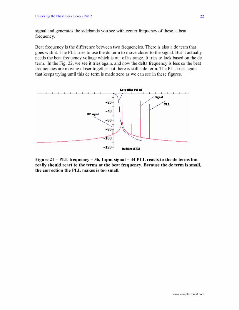
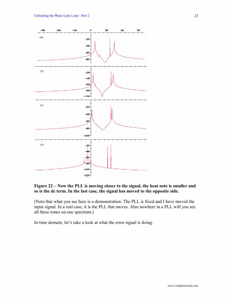
( )1.8 1PO nω ω ζ∆ = + (34) For zeta = .707, the most common figure, the pull-out frequency is app. three times the natural frequency. So if natural frequency of a loop is 10 kHz, then the frequency step can be as large as 30 kHz and the PLL will still maintain lock, i.e. no data would be lost. As long as the input frequency is within the lock range, the PLL can lock on to the incoming frequency fairly quickly. But there are cases, where even if the frequency is fairly far away the PLL may still be able to �walk up� to the incoming frequency and start tracking it. It takes longer but can be done. Let�s take a look at how this may be done. In Fig 21(a) below, we show a case, where PLL signal is moving towards the input signal. The signal is assumed to be out of the PLL range. This configuration gives rise to a FM modulation between the PLL and input



22

signal and generates the sidebands you see with center frequency of these, a beat frequency. Beat frequency is the difference between two frequencies. There is also a dc term that goes with it. The PLL tries to use the dc term to move closer to the signal. But it actually needs the beat frequency voltage which is out of its range. It tries to lock based on the dc term. In the Fig. 22, we see it tries again, and now the delta frequency is less so the beat frequencies are moving closer together but there is still a dc term. The PLL tries again that keeps trying until this dc term is made zero as we can see in these figures.

Figure 21 � PLL frequency = 36, Input signal = 44 PLL reacts to the dc terms but really should react to the terms at the beat frequency. Because the dc term is small, the correction the PLL makes is too small.



23

Figure 22 � Now the PLL is moving closer to the signal, the beat note is smaller and so is the dc term. In the last case, the signal has moved to the opposite side. (Note that what you see here is a demonstration. The PLL is fixed and I have moved the input signal. In a real case, it is the PLL that moves. Also nowhere in a PLL will you see all these tones on one spectrum.) In time domain, let�s take a look at what the error signal is doing.



24

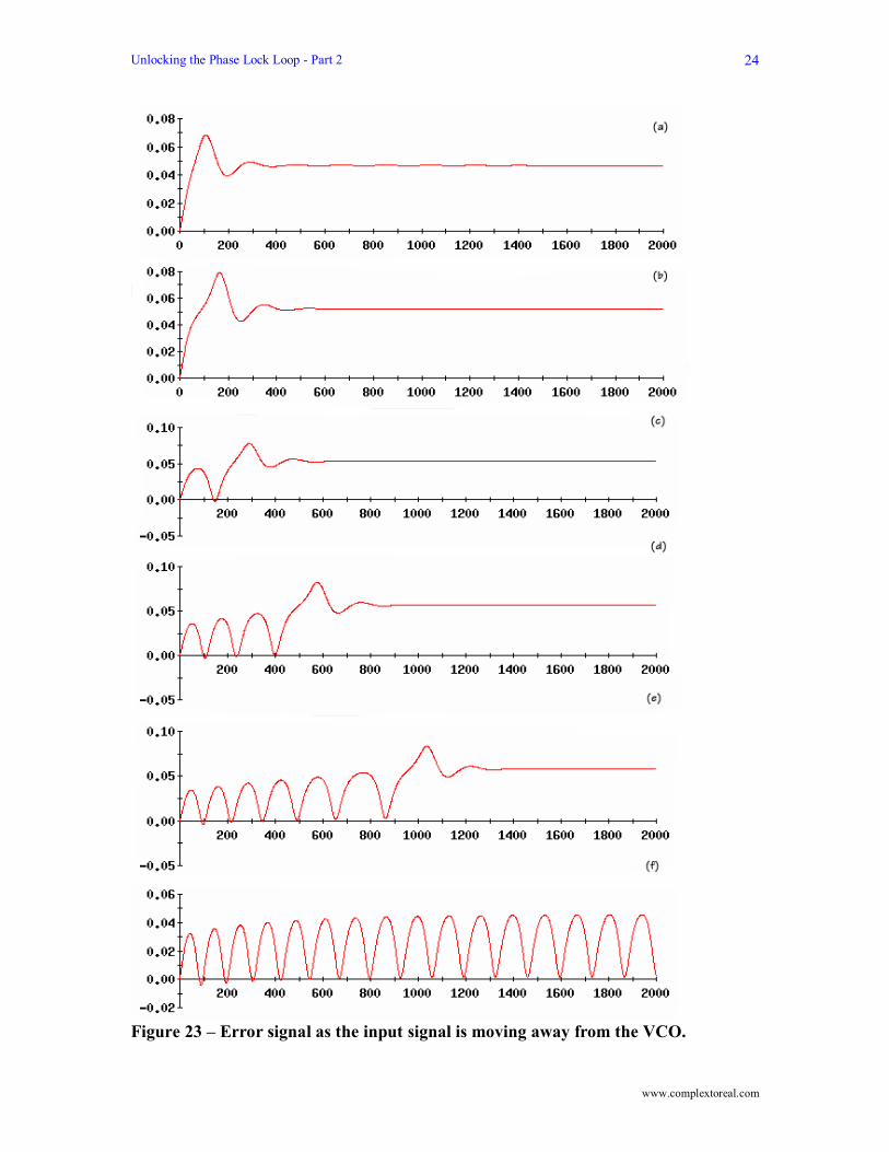
Figure 23 � Error signal as the input signal is moving away from the VCO.



25

The above figures show the response of a system with natural frequency of 1.0. The PLL is at 5.0 Hz. Figure 23 (a) shows the response when the input signal is 5.7 Hz. The error signal indicates that PLL is able to lock quickly. Figure 23 (b) shows response to an input signal at 5.75 Hz. Now the transient is a bit longer but lock is still obtained. In the figure (c), the input signal is at 5.8 Hz, now we see that that lock does not take place and the PLL goes through a second locking loop and it is taking longer to lock. This pattern continues as input frequency is moving away from PLL. At 5.9 Hz, the lock never takes place. This is called a pull-in process and although of interest academically, is not one we want to encounter in signal processing. We want to able to lock immediately and so should design a system that has a lock-in frequency well within what might be encountered. References: 1. Phaselock Techniques, Floyd Gardener, John Wiley & Sons, 2nd Edition 2. Phase-Locked Loop Circuit Design, Dan H. Wolaver, Prentice Hall, Ist Edition 3. Phase-Locked Loops: Design, Simulation, and Applications, Ronald E. Best, McGraw Hill, 4th Edition 4. Phase-Lock Basics, William Eagan, Wiley Inter-science, July 1998 ______________________________________________________

Copyright 1998, 2002 Charan Langton

I can be contacted at [email protected]

Other tutorials at www.complextoreal.com

Documents

Unlocking the Phase Lock Loop - Part 2biitcomm/research/references/Other... · Unlocking the Phase Lock Loop - Part 2 2 intuitively see that if a transient is large, the system will