Embed Size (px)
Citation preview

UNIVERZITET U BEOGRADU
MATEMATICKI FAKULTET
Hana Almoner Louka
Kvantna teorija informacija iasimptotika kvantnog potpisivanja
ugovora
DOKTORSKA DISERTACIJA
BEOGRAD, 2016

UNIVERSITY OF BELGRADE
FACULTY OF MATHEMATICS
Hana Almoner Louka
Quantum Information Theory andAsymptotics of Quantum Contract
Signing
DOCTORAL DISSERTATION
BELGRADE, 2016

AbstractThis thesis has been written under the supervision of my mentor dr. Vladimir Bozin at
the University of Belgrade in the academic year 2016. The topic of this thesis is quantuminformation theory, with special attention to quantum contract signing protocols. Thethesis is divided into four chapters. Chapter 1 gives introduction to Quantum mechanicsand necessary mathematical background. Chapter 2 is about quantum informationtheory. Quantum algorithms, including Schor’s and Grover’s, are described. Chapter3 deals with classical contract signing, and cryptography. Also discussed is the RSAalgorithm and BB84 quantum key distribution. Chapter 4 describes quantum signingprotocol, and proves, among other things, asymptotic behavior for probability of cheating.
Scientific field (naucna oblast): Mathematics (matematika)Narrow scientific field (uza naucna oblast): Analysis (analiza)UDC: 517.984+51-73/74+519.651
i

AbstraktOva teza napisana je pod supervizijom mog mentora dr. Vladimir Bozina na Uni-
verzitetu u Beogradu 2016. akademske godine. Tema ove disertacije je kvantna teorijainformacija, sa posebnim osvrtom na protokole kvantnog potpisivanja ugovora. Tezaje podeljena u cetiri poglavlja. Prvo poglavlje daje uvod u kvantnu mehaniku i relevan-tan matematicki aparat. Drugo poglavlje je o kvantnoj teoriji informacija. Opisani sukvantni algoritmi, ukljucujuci Sorov i Groverov. Trece poglavlje se bavi klasicnim potpi-sivanjem ugovora i kriptografijom. Govori se i o RSA algoritmu, kao i BB84 algoritmukvantnog dodeljivanja kljuceva. Cetvrto poglavlje opisuje protokol kvantnog potpisivanjaugovora, i dokazuje se, izmedju ostalog, asimptotika za verovatnocu varanja.
Scientific field (naucna oblast): Mathematics (matematika)Narrow scientific field (uza naucna oblast): Analysis (analiza)UDC: 517.984+51-73/74+519.651
ii

Podaci o mentoru i clanovima komisije:
MENTOR:
docent dr Vladimir Bozin
Matematicki fakultet,
Univerzitet u Beogradu
CLANOVI KOMISIJE :
redovni profesor dr Milos Arsenovic
Matematicki fakultet,
Univerzitet u Beogradu
redovni profesor dr Aleksandar Lipkovski
Matematicki fakultet,
Univerzitet u Beogradu
dr Nikola Paunkovic
Matematicki departman,
Univerzitet u Lisabonu
Datum odbrane:
iii

Acknowledgements
I would like to express my deepest gratitude to my advisor, dr Vladimir Bozin. I am
very grateful to the members of reading comitee, dr Nikola Paunkovic and Professors
Milos Arsenovic and Aleksandar Lipkovski for their valuable time. I would also like to
thank Prof. Zarko Mijajlovic for his support and interest in my professional develop-
ment and personal well-being. Finally, nothing would be possible without the support,
encouragement and motivation from my parents, my husband and family, to whom I
dedicate my work.
Hana LOUKA
iv

Contents
Abstract i
Abstrakt ii
Acknowledgements iv
1 Introduction to Quantum Mechanics 11.1 Linear Algebra . . . . . . . . . . . . . . . . . . . . . . . . . . . . . 1
1.1.1 Vector Space . . . . . . . . . . . . . . . . . . . . . . . . . . 21.1.2 Hilbert Space . . . . . . . . . . . . . . . . . . . . . . . . . . 31.1.3 Outer Product and Tensor Product . . . . . . . . . . . . . . 41.1.4 Linear Operators . . . . . . . . . . . . . . . . . . . . . . . . 51.1.5 Eigenvalues and Eigenvectors . . . . . . . . . . . . . . . . . 81.1.6 The Commutator and Anti-commutator . . . . . . . . . . . 8
1.2 Quantum Mechanics and State Spaces . . . . . . . . . . . . . . . . 91.2.1 Postulates of Quantum Mechanics . . . . . . . . . . . . . . 101.2.2 Observables and Projective Measurements . . . . . . . . . . 121.2.3 Density Operator Representation of Mixed and Pure States . 121.2.4 Separable States and Entangled States . . . . . . . . . . . . 131.2.5 EPR and Bell State . . . . . . . . . . . . . . . . . . . . . . . 14
2 Quantum Information Theory 182.1 Bit and quantum bit . . . . . . . . . . . . . . . . . . . . . . . . . . 182.2 Quantum Gates . . . . . . . . . . . . . . . . . . . . . . . . . . . . . 18
2.2.1 Single Qubit Gates . . . . . . . . . . . . . . . . . . . . . . . 182.2.2 Two Qubit Gates . . . . . . . . . . . . . . . . . . . . . . . . 232.2.3 Three Qubit Gates . . . . . . . . . . . . . . . . . . . . . . . 24
2.3 Universal Quantum Gates . . . . . . . . . . . . . . . . . . . . . . . 262.4 Quantum Algorithms . . . . . . . . . . . . . . . . . . . . . . . . . . 27
2.4.1 Shor’s Algorithm . . . . . . . . . . . . . . . . . . . . . . . . 272.4.1.1 General Steps of Shor’s Algorithm . . . . . . . . . 28
2.4.2 Grover’s Algorithm . . . . . . . . . . . . . . . . . . . . . . . 342.4.2.1 General Steps of Grovers Algorithm . . . . . . . . 35
1

LOUKA QIT and Asymptotics of Quantum Contract Signing 2
2.4.2.2 Grover iteration: How it works . . . . . . . . . . . 35
3 Cryptography and Contract Signing 403.1 Cryptography in General . . . . . . . . . . . . . . . . . . . . . . . . 40
3.1.1 RSA Algorithm . . . . . . . . . . . . . . . . . . . . . . . . . 413.1.1.1 Key Generation: . . . . . . . . . . . . . . . . . . . 433.1.1.2 Encryption and Decryption: . . . . . . . . . . . . . 44
3.2 Digital Signatures . . . . . . . . . . . . . . . . . . . . . . . . . . . . 453.3 Quantum Cryptography and Quantum Key Distribution . . . . . . 463.4 Contract Signing . . . . . . . . . . . . . . . . . . . . . . . . . . . . 47
4 Asymptotics of Quantum Contract Signing 494.1 Paunkovic-Bouda-Mateus Protocol . . . . . . . . . . . . . . . . . . 494.2 Necessity of Parameter Randomization . . . . . . . . . . . . . . . . 514.3 Asymptotic behaviour . . . . . . . . . . . . . . . . . . . . . . . . . 57
Bibliography 61

Chapter 1
Introduction to QuantumMechanics
Quantum Mechanics is a theory which describes nature most closely. For ourwork, we need to introduce some basic notions from this theory, and first weneed to review the relevant part of mathematics, and introduce notation which isstandard in this context, but is more used by physicists than mathematicians.In quantum mechanics (QM) vector space plays an important role because QM isa linear theory.
1.1 Linear Algebra
In this section we review some basic concepts from linear algebra, related withquantum mechanics. The literature used is [36, pg. 62-65],[5],[7, pg. 21], [4, pg. 199-200],[18, pg.61],[30],[1],[32], [44],[3].The standard notation which is used for concepts from linear algebra in the studyof quantum mechanics is summarized in following table:
Symbol Discribtion
z∗ Complex conjugate of the complex number z.(1 + i)∗ = 1− i
|ψ〉 Vector. Also known as a ket.〈ψ| Vector dual to |ψ〉. Also known as a bra.〈ψ|ϕ〉 Inner product between the vectors |ϕ〉 and |ψ〉
|ψ〉 ⊗ |ϕ〉, |ψ〉|ϕ〉, |ψϕ〉 Tensor product of |ψ〉 and |ϕ〉|ψ〉〈ϕ| Outer product between |ψ〉 and |ϕ〉B⊗n n fold tensor product of B with itselfB∗ Complex conjugate of the B matrix.BT Transpose of the B matrix.B† Hermitian conjugate or adjoint of the B matrix.[
a bc d
]†=
[a∗ c∗
b∗ d∗
]〈ψ|B|ϕ〉 Inner product between |ψ〉 and B|ϕ〉.
Equivalently, inner product between B†|ψ〉 and |ϕ〉.|+〉 1√
2(|0〉+ |1〉)
|−〉 1√2(|0〉 − |1〉)
1

LOUKA QIT and Asymptotics of Quantum Contract Signing 2
1.1.1 Vector Space
Definition 1.1. A vector space V is a set of objects called vectors (denoted by|ψ1〉, |ψ2〉, . . . ) and a set of numbers called scalars (denoted by α, β, γ, . . . ) withtwo operations, the operation ”addition”, denoted by ” + ”, and the operation”scalar multiplication”, usually denoted by a dot ”.”. If the scalars are real num-bers, we have a real vector space; if the scalars are complex numbers, we have acomplex vector space. The set must be closed under vector addition and scalarmultiplication.
Vector addition must have these properties:
• |ψ1〉+ |ψ2〉 = |ψ2〉+ |ψ1〉;
• |ψ1〉+ (|ψ2〉+ |ψ3〉) = (|ψ1〉+ |ψ2〉) + |ψ3〉;
• There exists a unique zero vector |0〉 such that: |ψ1〉+ |0〉 = |ψ1〉;
• For any vector |ψ1〉 there exists a unique vector | − ψ1〉 such that:
|ψ1〉+ | − ψ1〉 = |0〉
Scalar multiplication must have these properties:
• It is distributive with respect to vector addition and scalar addition:α(|ψ1〉+ |ψ2〉) = α|ψ1〉+ α|ψ2〉 and (α + β)|ψ1〉 = α|ψ1〉+ β|ψ1〉;
• It is associative with respect to ordinary scalar multiplication:α(β|ψ1〉) = (αβ)|ψ1〉;
• Multiplication by the scalars 0 and 1 yields the expected: 0|ψ1〉 = |0〉and 1|ψ1〉 = |ψ1〉.
Usually, a vector space over C is called a complex vector space and a vector spaceover R is called a real vector space. We use complex vector space in quantummechanics, and often call vectors ”states”.
Definition 1.2. A linear combination of a set of vectors {|ψi〉|1 ≤ i ≤ n} is givenby
α1|ψ1〉+ α2|ψ2〉+ α3|ψ3〉+ · · ·+ αn|ψn〉
where {αi|1 ≤ i ≤ n} is a set of complex coefficients .
Definition 1.3. A set of vectors {|ψi〉|1 ≤ i ≤ n} is linearly independent if nonontrivial linear combination (i.e. such that not all αi are zero) is a zero vector,and we say that these vectors are linearly independent.
Definition 1.4. The dimension of a vector space is equal to the maximal numberof linearly independent vectors.
Definition 1.5. A subspace V0 of a vector space V is a non-empty subset of Vwhich satisfies the following two requirements:
• For any pair |φ1〉, |φ2〉 in V0, |φ1〉+ |φ2〉 is in V0;
• For any |φ1〉 in V0 and any scalar α, α|φ1〉 is in V0.

LOUKA QIT and Asymptotics of Quantum Contract Signing 3
Definition 1.6. A spanning set for a vector space is a set of vectors {|ψ1〉, |ψ2〉, . . . , |ψn〉}such that any vector |ψ〉 in the vector space can be written as a linear combination|ψ〉 =
∑i αi|ψi〉 of vectors in that set.
Definition 1.7. Let V denote a vector space and S = {|φ1〉, |φ2〉, . . . , |φn〉} asubset of V . S is called a basis for V if the following is true:
1. S spans V ;
2. S is linearly independent.
1.1.2 Hilbert Space
Definition 1.8. The inner product (also called scalar product or dot product) oftwo vectors |ψ〉 and |φ〉 is a complex number, written 〈ψ|φ〉, assigned to each pairof vectors and with the following properties:
• 〈ψ|φ〉 = 〈φ|ψ〉∗ (Hermitian symmetric);
• 〈ψ|ψ〉 ≥ 0 (nonnegative);
• 〈ψ|ψ〉 = 0↔ |ψ〉 = |0〉 (positive definite);
• 〈ψ|(α|φ〉+ β|χ〉) = α〈ψ|φ〉+ β〈ψ|χ〉.
Definition 1.9. The length of a vector |ψ〉 (also called the norm of |ψ〉) is equalthe square root of 〈ψ|ψ〉 and is denoted by |ψ|.
In this way, given an inner product, the associated norm | · | on V is defined by
|x| =√〈x|x〉
and also, an associated metric can be defined by
d(x, y) = |x− y|
Definition 1.10. A set of non-zero vectors {|v1〉, |v2〉, ..., |vn〉} is said to be mu-tually orthogonal if 〈vi|vj〉 = 0 for all i 6= j.Note that if |0〉 and |1〉 are orthogonal vectors (notation we will use for qubits),then 〈0|1〉 = 〈1|0〉 = 0.The set is called orthonormal if additionally every vector in the set is a unit vector.Thus a set of vectors {|v1〉, |v2〉, ..., |vn〉} is orthonormal if and only if:
〈vi|vj〉 =
{0 if i 6= j
1 if i = j
Definition 1.11. A vector space together with an inner product is called an innerproduct space or a pre-Hilbert space.
Proposition 1. ([25], Theorem 3 (Pythagorean Theorem)) If x and y are orthog-onal vectors, then
|x+ y|2 = |x|2 + |y|2
LOUKA QIT and Asymptotics of Quantum Contract Signing 4
Proof.
|x+ y|2 = 〈x+ y|x+ y〉= |x|2 + 2〈x|y〉+ |y|2
= |x|2 + |y|2
Definition 1.12. A sequence of elements xn of an inner product space with asso-ciated norm and metric is called a Cauchy sequence if, for every ε > 0, there existsan n0 such that for all k,m ≥ n0, |xk − xm| < ε.
Definition 1.13. A Hilbert space H is a vector space with an inner product andassociated norm and metric such that every Cauchy sequence in H has a limit inH .
A pre-Hilbert space is a Hilbert space if and only if it is a complete normed space(i.e. a Banach space) under the norm associated with the inner product1.A finite dimensional pre-Hilbert space is always a Hilbert space, and this is thecase we will deal with mostly in this thesis.
1.1.3 Outer Product and Tensor Product
Definition 1.14. For a finite-dimensional vector space outer product between ket|ψ〉 and bra 〈φ| can be understood as:
|ψ〉〈φ| =
φ0
φ1
φ2...φn
[ψ0 ψ1 ψ2 · · · ψn]
=
ψ0φ0 ψ0φ1 ψ0φ2 . . . ψ0φnψ1φ0 ψ1φ1 ψ1φ2 . . . ψ1φn
......
.... . .
...ψnφ0 ψnφ1 ψnφ2 . . . ψnφn
Below, we list a few examples (using qubit notation for the standard basis of atwo dimensional space, {|0〉, |1〉}) :
|0〉〈0| =[10
] [1 0
]=
[1 00 0
]
|0〉〈1| =[10
] [0 1
]=
[0 10 0
]|1〉〈0| =
[01
] [1 0
]=
[0 01 0
]|1〉〈1| =
[01
] [0 1
]=
[0 00 1
]Definition 1.15. Tensor product H1⊗H2 of Hilbert spacesH1 andH2 is a Hilbertspace consisting of elements |ψ〉 ⊗ |φ〉 (with |ψ〉 ∈ H1 and |φ〉 ∈ H2 ) and theirlinear combinations. The operations in the space obey the following rules:
1 a normed space is a Banach space if every Cauchy sequence in normed space converges

LOUKA QIT and Asymptotics of Quantum Contract Signing 5
1. α(|ψ〉 ⊗ |φ〉) = (α|ψ〉)⊗ |φ〉 = |ψ〉(α|φ〉);
2. (|ψ1〉+ |ψ2〉)⊗ |φ〉 = |ψ1〉 ⊗ |φ〉+ |ψ2〉 ⊗ |φ〉;
3. |ψ〉 ⊗ (|φ1〉+ |φ2〉) = |ψ〉 ⊗ |φ1〉+ |ψ〉 ⊗ |φ2〉;
4. The inner product of two vectors |ψ1〉 ⊗ |φ1〉 and |ψ2〉 ⊗ |φ2〉 in H1 ⊗ H2 isgiven by 〈ψ1φ1|ψ2φ2〉 = 〈ψ1|ψ2〉〈φ1|φ2〉.
Example 1.1. Consider tensor product of two qubits (vectors from two dimen-sional space):
|ψ1〉 = α1|0〉+ β1|0〉 and |ψ2〉 = α2|0〉+ β2|0〉
Tensor product of |ψ1〉 and |ψ2〉 is:
|ψ1〉 ⊗ |ψ2〉 = (|α1|0〉+ β1|1〉)⊗ (α2|0〉+ β2|1〉)= α1α2|00〉+ α1β2|01〉+ β1α2|10〉+ β1β2|11〉
where
|00〉 = |0〉 ⊗ |0〉|01〉 = |0〉 ⊗ |1〉|10〉 = |1〉 ⊗ |0〉|11〉 = |1〉 ⊗ |1〉.
Tensor product is also defined for matrices. For example, tensor product of the
following two matrices X =
[x11 x12
x21 x22
]and Y =
[y11 y12
y21 y22
]is given by
X ⊗ Y =
[x11Y x12Yx21Y x22Y
]=
x11y11 x11y12 x12y11 x12y12
x11y21 x11y22 x12y21 x12y22
x21y11 x21y12 x22y11 x22y12
x21y21 x21y22 x22y21 x22y22
1.1.4 Linear Operators
In this chapter, we will sometimes refer to vectors as ”states” (for convenience andbecause of a later use in quantum mechanic application).
Definition 1.16. If A is an operator mapping states to states, such that forarbitrary pair of states |ψ1〉 and |ψ2〉 and for any two complex numbers c1 and c2:
A(c1|ψ1〉+ c2|ψ2〉) = c1A|ψ1〉+ c2A|ψ2〉
then A is said to be a a linear operator. More generally, a linear operator A actson a linear combination of states/vectors as follows:
A(∑
i
ci|ψi〉)
=∑i
ciA(|ψi〉
)Important linear operators on any vector space V are the corresponding unit oridentity operator, I = IV and the zero operator 0. For the unit operator, IV |ψ〉 =|ψ〉 for all vectors |ψ〉, and for the zero operator, 0|ψ〉 = 0.

LOUKA QIT and Asymptotics of Quantum Contract Signing 6
Definition 1.17. An operator A is positive if 〈ψ|A|ψ〉 is real and
〈ψ|A|ψ〉 ≥ 0
for any vector |ψ〉.Definition 1.18. The Hermitian adjoint of operator B is denoted by B† and isdefined by the following property:
〈φ|B†|ψ〉 = 〈ψ|B|φ〉∗.
To compute the Hermitian adjoint of any expression, we take the complex con-jugate of all constants in the expression, replace all bras by kets and vice versaand replace operators by their adjoints. Also, just like transposition, Hermitianadjoint of a product reverses order, i.e. (AB)† = B†A†. For matrices, Hermitianadjoint of a matrix is the complex conjugate of the transpose matrix.
Definition 1.19. The operator B is Hermitian or self adjoint if it is equal to itsHermitian adjoint, i.e. if B = B†.
For example the Pauli operator Y = −i|0〉〈1|+ i|1〉〈0| is Hermitian, since Y † =(−i|0〉〈1|+ i|1〉〈0|) = −i|0〉〈1|+ i|1〉〈0| = Y .
Definition 1.20. The inverse of an operator B is denoted by B−1. This operatorsatisfies BB−1 = B−1B = I, where I is the identity operator.
Definition 1.21. An operator is said to be unitary if its adjoint is equal to itsinverse. Unitary operators are often denoted using the symbol U . They satisfy
U † = U−1 ←→ UU † = U †U = I
For example the Pauli operators are both Hermitian and unitary.Unitary operators preserve the inner (scalar) product:
Proposition 2. The inner product of U |φ〉 and U |ψ〉 is the same as the innerproduct of |ψ〉 and |φ〉.Proof. (U |ψ〉, U |φ〉) = 〈ψ|U †U |φ〉 = 〈ψ|I|φ〉 = 〈ψ|φ〉
Definition 1.22. An operator B is said to be normal if
B†B = BB†.
Unitary and Hermitian operators are examples of normal operators.
Example 1.2. If A is Hermitian then the operator eiA is unitary.Since:
eiA = I + iA+i2
2!A2 + · · ·+ in
n!An + . . .
(eiA)† = I + (−i)A+(−i)2
2!A2 + · · ·+ (−i)n
n!An + . . . = e−iA
and
e−iAeiA = I.

LOUKA QIT and Asymptotics of Quantum Contract Signing 7
Definition 1.23. An operator P is said to be a projector if
P 2 = P.
If P is also Hermitian, then it is called an orthogonal projector.
Projectors act as identity operator on some subspace of the vector space. Orthog-onal projectors map vectors orthogonal to all vectors in that space to zero.
Definition 1.24. A tensor product of two linear operators, A acting on vectorspace V and B acting on vector space W , is the operator A⊗B acting on V ⊗W ,so that
A⊗B(|φ〉 ⊗ |ψ〉) = (A|φ〉)⊗ (B|ψ〉)
Definition 1.25. The trace of an operator A on an n-dimensional space H is thesum of the diagonal elements of an operator:
Tr(A) =n∑i
〈ψi|A|ψi〉
for any orthonormal set of basis vectors {|ψi〉}
For any two operators A and B on a Hilbert space we have:
• Tr(αA) = αTr(A)
• Tr(A+B) = Tr(A) + Tr(B)
• Tr(AB) = Tr(BA)
Example 1.3. Lets compute trace of an operator expressed in the orthonormalbasis {|0〉, |1〉} as
A = 2i|0〉〈0|+ 3|0〉〈1| − 2|1〉〈0|+ 4|1〉〈1|
We find the trace by computing
Tr(A) =∑i
〈ψi|A|ψi〉 = 〈0|A|0〉+ 〈1|A|1〉
〈0|A|0〉 = 〈0|(2i|0〉〈0|+ 3|0〉〈1| − 2|1〉〈0|+ 4|1〉〈1|
)|0〉
= 2i〈0|0〉〈0|0〉+ 3〈0|0〉〈1|0〉 − 2〈0|1〉〈0|0〉+ 4〈0|1〉〈1|0〉= 2i〈0|0〉〈0|0〉+ 0 = 2i
〈1|A|1〉 = 〈1|(2i|0〉〈0|+ 3|0〉〈1| − 2|1〉〈0|+ 4|1〉〈1|
)|1〉
= 2i〈1|0〉〈0|1〉+ 3〈1|0〉〈1|1〉 − 2〈1|1〉〈0|1〉+ 4〈1|1〉〈1|1〉= 4〈1|1〉〈1|1〉 = 4
Hence the trace is 〈0|A|0〉+ 〈1|A|1〉 = 2i+ 4.

LOUKA QIT and Asymptotics of Quantum Contract Signing 8
1.1.5 Eigenvalues and Eigenvectors
Definition 1.26. A state vector |ψ〉 is said to be an eigenvector (also called aneigenket or eigenstate) of an operator A if the application of A to |ψ〉 gives
A|ψ〉 = λ|ψ〉
where λ is a complex number, called an eigenvalue of A. This equation is knownas the eigenvalue equation, or eigenvalue problem, for the operator A (see [52]).
To find eigenvalues and eigenvectors for an operator A represented as an n by nmatrix, the first step in this process is using what is known as the characteristicequation. The characteristic equation for an operator A is defined to be det|A −λI| = 0 where λ is an unknown variable, I is the identity matrix and det denotesthe determinant of the n by n matrix A− λI.The values λi of roots (solutions) of the characteristic equation are the eigenvaluesof the operator A.To find the associated eigenvectors, we solve the equation (A− λiI)v = 0; for i =1, . . . n.The set of all eigenvectors for given eigenvalue λ is called an eigenspace. Whenλ is a simple zero of characteristic equation, i.e. nondegenerate eigenvalue, theeigenspace for λ is one dimensional.Eigenvalues of an operator are sometimes called the spectrum of that operator.Now we give some proprieties of eigenvalues and eigenvectors for unitary andHermitian operators (see [32]).The eigenvalues and eigenvectors of a unitary operator satisfy the following:
• The eigenvalues of a unitary operator are complex numbers with modulus 1.
• A unitary operator with nondegenerate eigenvalues has mutually orthogonaleigenvectors.
The eigenvalues and eigenvectors of a Hermitian operator also satisfy the followingimportant properties:
• The eigenvalues of a Hermitian operator are real.
• The eigenvectors of a Hermitian operator corresponding to different eigen-values are orthogonal.
1.1.6 The Commutator and Anti-commutator
For litereature for this part, see for instance [24].
Definition 1.27. The commutator of two operators is [A,B] = AB − BA. Twooperators commute/are commutable if [A,B] = 0.
Definition 1.28. The anti-commutator of two operators A and B is defined by
{A,B} = AB +BA.
We say that A anti-commutes with B if {A,B} = 0.

LOUKA QIT and Asymptotics of Quantum Contract Signing 9
We have the following properties:
• Any operator commutes with itself:[A,A] = 0.
• The commutator of A, B is the negative of the commutator of B, A:[A,B] = −[B,A].
• The commutator of two Hermitian operators is anti-Hermitian :[A,B]† = (AB)† − (BA)† = B†A† − A†B† = −(AB −BA) = −[A,B].
• The anti-commutator of two Hermitian operators is Hermitian:{A,B}† = (AB)† + (BA)† = B†A† + A†B† = BA+ AB = {A,B}.
• [A,B]
2+{A,B}
2=AB −BA
2+AB +BA
2= AB
Note that if A and B are Hermitian, and |ψ〉 is some state, then 〈ψ|{A,B}|ψ〉 isreal and 〈ψ|[A,B]|ψ〉 is an imaginary number. So
|〈ψ|{A,B}|ψ〉|2 + |〈ψ|[A,B]|ψ〉|2 = 4|〈ψ|AB|ψ〉|2 (1.1)
If two Hermitian operators acting on a finite dimensional Hilbert space commute,then there is a common orthonormal basis in which both are represented as diag-onal matrices. This is not the case with the anticommuting operators.In physics, non-commuting Hermitian operators are important, as they corre-spond to observables that cannot be measured at the same time. Note thatsince by the Cauchy-Schwartz inequality2, for Hermitian operators |〈ψ|AB|ψ〉|2 ≤〈ψ|A2|ψ〉〈ψ|B2|ψ〉, we have from (1.1) the following bound for the commutator ofHermitian operators:
|〈ψ|[A,B]|ψ〉|2 ≤ 4〈ψ|A2|ψ〉〈ψ|B2|ψ〉,
which is related with the so called uncertainty principle of quantum mechanics fornon-commuting observables.
1.2 Quantum Mechanics and State Spaces
In this section we will give a general and quick introduction to quantum mechan-ics, which is basis for the sequel.
In the early 20th century a new science known as quantum mechanics appeared,see [16, pg. 188]. It is a mathematical theory that can describe the behaviorof objects that are roughly 10,000,000,000 times smaller than a typical humanbeing, typically of atomic size, describing for instance movement of electrons withinatoms, see [39]. In this quantum world we need to forget everything we know aboutour daily experience: relation between action and reaction, reality, certainty andmuch more. Quantum mechanics is a separate science, it has its own rules anddeals with physics which is impossible to explain in any classical way (for instance,the mentioned movement of electrons or photons within the atom).
2 Cauchy-Schwartz inequality states that |〈x|y〉|2 ≤ |x|2|y|2.

LOUKA QIT and Asymptotics of Quantum Contract Signing 10
1.2.1 Postulates of Quantum Mechanics
In quantum mechanics a state space is a complex complete inner product space(i.e. Hillbert space that will be referred to as H) corresponding to a physicalsystem, and the following postulate holds (see[36, pp. 88-102],[35, pp. 80-83]):
Postulate 1: Associated to any isolated physical system is a complex Hilbertspace known as the state space of the system. The system is completelydescribed by its state vector, which is a unit vector in the system’s statespace.
For example an arbitrary state vector in a two dimensional state space can bewritten as |ψ〉 = a|0〉 + b|1〉 with a, b ∈ C, and |ψ〉 must be a unit vector (i.e.〈ψ|ψ〉 = 1 or |a|2 + |b|2 = 1).In general, a scalar multiple of a state vector by a number α with |α| = 1 representsthe same physical ”state”.
Postulate 2: The evolution of a closed quantum system is described by a unitarytransformation. That is, the state |ψ1〉 of the system at time t1 is relatedto the state |ψ2〉 of the system at time t2 by a unitary operator U whichdepends only on the times t1 and t2,
|ψ2〉 = U |ψ1〉
Example 1.4. Let |ψ〉 = 1|0〉 + 0|1〉 =
[10
], where |0〉 =
[10
], |1〉 =
[01
],
〈0| =[1 0
], 〈1| =
[0 1
]and U = 1√
2
[1 11 −1
]We check that U is unitary, i.e. that U †U = I:
U †U =1√2
1√2
[1 11 −1
] [1 11 −1
]=
1
2
[2 00 2
]=
[1 00 1
]= I
|ψ2〉 = U |ψ1〉 =1√2
[1 11 −1
] [10
]=
1√2
[11
]=
1√2|0〉+
1√2|1〉
Postulate 2′: The time evolution of a closed quantum system is described bySchrodinger equation:
i~d|ψ〉dt
= H|ψ〉
where ~ is Planck’s constant, and H is a fixed Hermitian operator known asthe Hamiltonian of the closed system.
Postulate 3: Quantum measurement is described by a set of operators {Mm}acting on the state space of the system, where m refers to the measurementoutcomes that may occur in the experiment.If the state of the quantum system is |ψ〉 immediately before the measure-ment, then the probability p that result m occurs is given by:
p(m) = 〈ψ|M †mMm|ψ〉

LOUKA QIT and Asymptotics of Quantum Contract Signing 11
The state of the system after the measurement is:
|ψ′〉 =Mm|ψ〉√〈ψ|M∗
mMm|ψ〉=Mm|ψ〉√p(m)
Furthermore the measurement operators satisfy the completeness equation:∑m
M †mMm = I,
where I is the identity operator on H. The completeness equation expressesthe fact that probabilities sum to 1:∑
m
p(m) =∑m
〈ψ|M †mMm|ψ〉 = 〈ψ|ψ〉 = 1
Example 1.5. Consider measuring a qubit basis {|0〉, |1〉}, and suppose that statebefore measurement is a|0〉〈0|+ b|1〉〈1|.Measurement operators are:
M0 = |0〉〈0| =[10
] [1 0
]=
[1 00 0
]M1 = |1〉〈1| =
[01
] [0 1
]=
[0 00 1
]
Measurement probabilities are:
p(0) = 〈ψ|M †0M0|ψ〉 = 〈ψ|M0|ψ〉 =
[a b
]×[1 00 0
]×[ab
]= |a|2
p(1) = 〈ψ|M †1M1|ψ〉 = 〈ψ|M1|ψ〉 =
[a b
]×[0 00 1
]×[ab
]= |b|2
The possible states after measurement are:
M0|ψ〉√p(0)
=a|0〉√|a|2
=a
|a||0〉
M1|ψ〉√p(1)
=b|1〉√|b|2
=b
|b||1〉
Postulate 4: The state space of a composite system consisting of n componentsis the tensor product of the state spaces of the components. If the component

LOUKA QIT and Asymptotics of Quantum Contract Signing 12
system i has state |ψi〉 the composite system state is:
|ψ〉 = |ψ1〉 ⊗ |ψ2〉 ⊗ · · · ⊗ |ψn〉
1.2.2 Observables and Projective Measurements
In quantum mechanics, measurements are often expressed in terms of observables,which correspond to projective measurements.
Definition 1.29. Projective measurement is described by a Hermitian operatorA. It can be expressed as a sum
A =∑m
λmPm,
where each λm is a real number, representing value of the observable correspond-ing to measurement outcome m, and each Pm is an orthogonal projector. Thecorresponding measurement has measurement operators Mm = Pm.
Not all measurements are projective. For example, measurement with two out-comes and measurement operators M1 = 1√
2I, M2 = 1√
2I is not projective. How-
ever, every measurement can be expressed as a projective measurement in a com-posite system, after some unitary transformation (see [36, ch. 2.2.8]).
1.2.3 Density Operator Representation of Mixed and Pure States
This section is based on [32].Suppose we have a situation, where a physical system is in state |ψi〉 with prob-ability pi. This is called a classical mixture of quantum states |ψi〉, each withcorresponding probability pi.It is represented by a so called density matrix of a mixture, defined by:
ρ =n∑i=1
pi|ψi〉〈ψi|
such that∑
i pi = 1, where n is the (arbitrary) number of terms in the mixture.We list several properties of the density operator:
• The density operator is Hermitian: ρ = ρ†;
• The density operator is positive: ρ ≥ 0;
• The density operator is normalized: Tr(ρ) = 1.
Let’s begin with the pure states, i.e. when there is only one state in the mixture.The density operator for pure state is ρ = |ψ〉〈ψ|. A more general type of state
is called mixed ρ =n∑i
pi|ψi〉〈ψi|, where |ψi〉 represent states as vectors, that are
not necessarily orthogonal. The number n could be anything, and is not limitedby the dimension of H. The n numbers (or ”weights”) pi are nonzero and satisfy
the relations pi > 0;∑
pi = 1 and, when n > 1, Tr(ρ2) < 13.
There are two simple tests to determine whether ρ describes a mixed state or not:3mixed state is a so called statical ensemble {(|ψ1〉, p1), (|ψ2〉, p2), . . . , (|ψn〉, pn)}
LOUKA QIT and Asymptotics of Quantum Contract Signing 13
• mixed state: ρ2 6= ρ; pure state: ρ2 = ρ
• mixed state: Tr(ρ2) < 1; pure state: Tr(ρ2) = 1
Example 1.6. A system is found to be in the state
|ψ〉 =1√5|0〉+
2√5|0〉
The the density operator is
ρ = |ψ〉〈ψ| =( 1√
5|0〉+
2√5|0〉)( 1√
5〈0|+ 2√
5〈0|)
=1
5|0〉〈0|+ 2
5|0〉〈1|+ 2
5|1〉〈0|+ 4
5|1〉〈1|
In the {|0〉, |1〉} basis the density matrix is
[ρ] =
[〈0|ρ|0〉 〈0|ρ|1〉〈1|ρ|0〉 〈1|ρ|1〉
]=
[15
25
25
45
]
The trace is just the sum of the diagonal elements. In this case
Tr(ρ) =1
5+
4
5= 1
Lets square the matrix:
ρ2 =
[15
25
25
45
][15
25
25
45
]=
[ 125
+ 425
225
+ 825
225
+ 825
425
+ 1225
]=
[ 525
1025
1025
2025
]=
[15
25
25
45
]= ρ
Since ρ2 = ρ, it follows that Tr(ρ2) = 1 and this is a pure state.
1.2.4 Separable States and Entangled States
Suppose we have a composite system which consists of two subsystems, H1 andH2 (see [34, pp. 61-86][40] and [17]). We can divide state vectors into two groups:
Entangled States : There is no |ψ1〉 ∈ H1, |ψ2〉 ∈ H2 such that |ψ〉 = |ψ1〉 ⊗ |ψ2〉
Separable States : There exists |φ1〉 ∈ H1, |φ2〉 ∈ H2 such that |φ〉 = |φ1〉 ⊗ |φ2〉
So, a state vector |ψ〉 is called separable iff it can be written as |ψ〉 = |ψ1〉 ⊗ |ψ2〉,otherwise it is entangled.
• For example a pure separable state is
|ψ〉 =|00〉+ 2|01〉+ |10〉+ 2|11〉√
10=|0〉+ |1〉√
2⊗ |0〉+ 2|1〉√
5
.
• Examples of pure entangled states are |φ±〉 = 1√2(|00〉±|11〉), |ψ±〉 = 1√
2(|01〉±
|10〉), called ”Bell states” or ”EPR states”.

LOUKA QIT and Asymptotics of Quantum Contract Signing 14
A mixed state ρ is called separable (not entangled) iff it can be written as a convexcombination of pure product states:
ρ =∑i
pi|ψi〉〈ψi| ⊗ |φi〉〈φi| =∑i
piρψi ⊗ ρ
φi ,
where |ψi〉 ∈ H1 and |φi〉 ∈ H2 are state vectors of subsystems 1 and 2 respectively,
and numbers pi > 0 are such that∑i
pi = 1
1.2.5 EPR and Bell State
Suppose we have a pair of photons with their polarization states (vertical andhorizontal) represented by vectors in two dimensional Hilbert spaces with basisvectors {|0〉1, |1〉1} and {|0〉2, |1〉2} respectively, which is generated by a physicalprocess of annihilation of electron and positron. This process will give an entangledstate known as an EPR pair (also called a Bell state), represented as
|ψ−〉 =1√2
(|0〉1 ⊗ |1〉2 − |1〉1 ⊗ |0〉2
)=
1√2
(|−〉1 ⊗ |+〉2 − |+〉1 ⊗ |−〉2
),
where
|+〉 =1√2
(|0〉+ |1〉), |−〉 =1√2
(|0〉 − |1〉), |0〉 =
[10
]and |1〉 =
[01
].
Of the two photons, one will be measured by Alice, and another by Bob, andthey are in distant laboratories receiving one photon each. Both can choose whatto measure on their photons. Suppose we have 4 observables, AA, RA, AB, RB,where the lower index denotes Alice or Bob, and for each there is the ”accept”observable4
A = 1.|1〉〈1|+ 0.|0〉〈0|
and the ”reject” observable
R = 1.|+〉〈+|+ 0.|−〉〈−|.
Here {|+〉, |−〉} will be the the ”reject basis”, {|0〉, |1〉} will be the the ”acceptbasis” that is being measured.If both measure the same basis, they will get the opposite results, for instance ifthey measure the ”accept” observable, and the result is |1〉 for Bob, result will be|0〉 for Alice (also if Alice gets |0〉 Bob will get |1〉). At the same time if Alice mea-sures the ”reject” observable she will know what Bob would get if he measured the”reject” observable. Since photons are distant, measurements of Bob (or Alice)on one photon should not influence local properties of the other photon. But byquantum mechanics, no one, neither Alice nor Bob, can measure both A and R at
4our names of observables here used correspond to cryptography protocol we will discuss in the lastchapter.

LOUKA QIT and Asymptotics of Quantum Contract Signing 15
the same time on their photons. But if Alice measures A and Bob measures R itseems that they have measured both in A and R for one particle, which is calledEinstein-Podolsky-Rosen (EPR) paradox, see [36].
It turns out that EPR paradox can be made more explicit.Let us denote |1〉φ = cos φ |1〉+sin φ |0〉, |0〉φ = −sin φ |1〉+cos φ |0〉 and considerthe observable
Pφ = 1.|1〉φ〈1|φ + 0.|0〉φ〈0|φ,
representing measurement of polarization for axes rotated by angle φ. Note that{|0〉φ, |1〉φ} is a basis of our Hilbert space. For φ = 0 we get |0〉, |1〉 respec-tively for |0〉φ, |1〉φ and for φ = π/4 we get |−〉, |+〉 respectively for |0〉φ, |1〉φ, so
P0 = A, Pπ/4 = R.
It can be checked that for all φ, |ψ−〉 = 1√2
(|0〉φ ⊗ |1〉φ − |1〉φ ⊗ |0〉φ
).
If Alice measures polarization angle α and Bob measures angle β on |ψ−〉, andAlice gets i, i ∈ {0, 1} and Bob gets j, j ∈ {0, 1}probability of that event is
|〈ψ−|i〉α ⊗ |j〉β|2.
But Alice’s result for angle β would be opposite of Bob’s. So for Alice’s photon tohave polarization 1 for angle α and 1 for angle β probability is |〈ψ−(|1〉α⊗|0〉β)|2,and have polarization 1 for α and 0 for β probability is |〈ψ−(|1〉α ⊗ |1〉β)|2.
|〈ψ−|(|1〉α ⊗ |1〉β)|2 =∣∣∣(〈0| ⊗ 〈1| − 〈1| ⊗ 〈0|√
2
)×(
(cos α |1〉+ sinα |0〉)⊗ (cos β |1〉+ sin β |0〉))∣∣∣2
Using notation |0〉 ⊗ |1〉 = |01〉 etc, we have
|〈ψ−|(|1〉α ⊗ |1〉β)|2 =∣∣∣(〈01| − 〈10|√
2
)×(cos α cos β |11〉+ cos α sin β |10〉
+ sin α cos β |01〉+ sinα sin β |00〉)∣∣∣2
=∣∣∣(〈01| − 〈10|√
2
)cos α cos β |11〉+
(〈01| − 〈10|√2
)cos α sin β |10〉
+(〈01| − 〈10|√
2
)sin α cos β |01〉+
(〈01| − 〈10|√2
)sinα sin β |00〉
∣∣∣2=∣∣∣ 1√
2
(cos α cos β 〈01|11〉 − cos α cos β 〈10|11〉
+ cos α sin β 〈01|10〉 − cos α sin β 〈10|10〉+ sin α cos β 〈01|01〉 − sin α cos β 〈10|01〉
+ sin α cos β 〈01|00〉 − sin α cos β 〈10|00〉)∣∣∣2
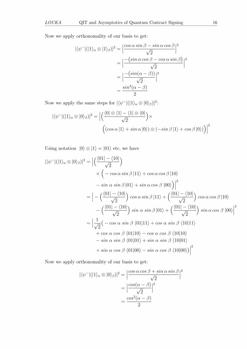
LOUKA QIT and Asymptotics of Quantum Contract Signing 16
Now we apply orthonomality of our basis to get:
|〈ψ−|(|1〉α ⊗ |1〉β)|2 =∣∣∣cos α sin β − sinα cos β√
2
∣∣∣2=∣∣∣−(sinα cos β − cos α sin β)√
2
∣∣∣2=∣∣∣−(sin(α− β))
√2
∣∣∣2=sin2(α− β)
2
Now we apply the same steps for |〈ψ−|(|1〉α ⊗ |0〉β)|2:
|〈ψ−|(|1〉α ⊗ |0〉β)|2 =∣∣∣(〈0| ⊗ 〈1| − 〈1| ⊗ 〈0|√
2
)×(
(cos α |1〉+ sinα |0〉)⊗ (−sin β |1〉+ cos β |0〉))∣∣∣2
Using notation |0〉 ⊗ |1〉 = |01〉 etc, we have
|〈ψ−|(|1〉α ⊗ |0〉β)|2 =∣∣∣(〈01| − 〈10|√
2
)×(− cos α sin β |11〉+ cos α cos β |10〉
− sin α sin β |01〉+ sinα cos β |00〉)∣∣∣2
=∣∣∣− (〈01| − 〈10|√
2
)cos α sin β |11〉+
(〈01| − 〈10|√2
)cos α cos β |10〉
−(〈01| − 〈10|√
2
)sin α sin β |01〉+
(〈01| − 〈10|√2
)sinα cos β |00〉
∣∣∣2=∣∣∣ 1√
2
(− cos α sin β 〈01|11〉+ cos α sin β 〈10|11〉
+ cos α cos β 〈01|10〉 − cos α cos β 〈10|10〉− sin α sin β 〈01|01〉+ sin α sin β 〈10|01〉
+ sin α cos β 〈01|00〉 − sin α cos β 〈10|00〉)∣∣∣2
Now we apply orthonomality of our basis to get:
|〈ψ−|(|1〉α ⊗ |0〉β)|2 =∣∣∣cos α cos β + sinα sin β√
2
∣∣∣2=∣∣∣cos(α− β)√
2
∣∣∣2=cos2(α− β)
2

LOUKA QIT and Asymptotics of Quantum Contract Signing 17
Figure 1.1: Bell inequality for Alice’s photon
From the figure (1.1) we see that the following formula (special case of Bell in-equalities) should hold for Alice’s photon (pθ denotes what would outcome be on
Alice’s photon if observable Pθ were measured):
prob (pθ1 = 1, pθ2 = 1) + prob (pθ2 = 0, pθ3 = 1) ≥ prob (pθ1 = 1, pθ3 = 1)
But setting θ1 = 0, θ2 = π/3 and θ3 = π/4 we get that it does not hold, since
prob (p0 = 1, pπ/3 = 1) + prob (pπ/3 = 0, pπ/4 = 1) = (cos2(π/3) + sin2(π/12))/2
prob (p0 = 1, pπ/4 = 1) = cos2(π/4)/2
but cos2(π/4) > cos2(π/3) + sin2(π/12). In this way, we see that naive interpre-tation of photons having ”local” properties does not hold in quantum mechanics,and this can be shown by a simple (in principle) experiment.

Chapter 2
Quantum Information Theory
Quantum information theory deals with specific aspects of quantum mechanics,and has played an important role in science in the last 20 years. There are practicalapplications in cryptography, and in theory, quantum computation is potentiallymuch more powerful than classical.
2.1 Bit and quantum bit
In a classical computer, the value of a bit can be either 0 or 1. In a quantumcomputer, a quantum bit (or qubit for short) can exist in a superposition of states|0〉 and |1〉, and is described by:
|ψ〉 = α|0〉+ β|1〉,
where α and β are complex numbers satisfying the normalization condition: |α|2 +|β|2 = 1, see [50, p. 208].An n-qubit state is represented as a normalized vector in 2n dimensional space,with basis vectors coressponding to all possible classical n-bit states,
|0 . . . 00〉, |0 . . . 01〉, . . . , |1 . . . 11〉.
2.2 Quantum Gates
Quantum gates are unitary transformations that act on one or several qubits, whileleaving the rest of the qubits the same, i.e. acting as some unitary transformationtensored with identity operator on the rest of the qubit spaces.Quantum gates are usually represented as matrices. A gate which acts on k qubitsis represented by a 2k×2k unitary matrix (see [48, pg. 63-69],[38, pp. 138-147],[43]and [23]).
2.2.1 Single Qubit Gates
A single qubit gate is a unitary operator which transforms a single qubit state
|ψ〉in to anther single qubit |ψout〉 = U |ψin〉, where |ψ〉 = α|0〉+ β|1〉 =
(αβ
).
Examples of single qubit gates include Pauli gates, Hadamard gate, phase gate orphase shift gate, rotation gates and square root of-NOT.
18

LOUKA QIT and Asymptotics of Quantum Contract Signing 19
1. Pauli Gates:
• Pauli X-Gate or NOT Gate: is defined as
X = σx =
[0 11 0
]It flips a bit from 0 to 1 and vice versa and is represented as
X|0〉 =
[0 11 0
]=
[10
]= |1〉
and
X|1〉 =
[0 11 0
]=
[01
]= |0〉
• Pauli Y-Gate is defined as:
σY = Y =
[0 −ii 0
]The Pauli-Y transformation is represented as
Y |0〉 =
[0 −ii 0
] [10
]= i
[01
]= i|1〉
and
Y |1〉 =
[0 −ii 0
] [01
]= −i
[10
]= −i|0〉
• Pauli Z-Gate, also known as Phase Flip is defined as:
σz = Z =
[0 −11 0
]
The Pauli-Z transformation keeps |0〉 unchanged and changes |1〉 to−|1〉 and is represented as
Z|0〉 =
[1 00 −1
] [10
]= |0〉
and
Z|1〉 =
[1 00 −1
] [01
]= |1〉
Note the following properties of Pauli matrices:
• tr(σx) = tr(σy) = tr(σz) = 0
• det(σx) = det(σy) = det(σz) = −1
• σ†x = σx
• σ†y = σy
• σ†z = σz

LOUKA QIT and Asymptotics of Quantum Contract Signing 20
The cyclic properties of Pauli matrices:
• σ2x = σ2
y = σ2z
• σxσy = −σyσx = iσz
• σyσz = −σzσy = iσx
• σzσx = −σxσz = iσy
• σxσyσz = iI
we can use the Dirac notation∑ij
|i〉Aij〈j| for writing the Pauli matrices:
• σx = |0〉〈1|+|1〉〈0| =[10
] [0 1
]+
[01
] [1 0
]=
[0 10 0
]+
[0 01 0
]=
[0 11 0
]• σy = −i|1〉〈0| + i|0〉〈1| = −i
[01
] [1 0
]+ i
[10
] [0 1
]=
[0 −ii 0
]+[
0 01 0
]=
[0 11 0
]• σz = |0〉〈0| − |1〉〈1| =
[10
] [1 0
]−[01
] [0 1
]=
[0 10 0
]−[1 00 0
]=[
0 −11 0
]2. Hadamard Gate: can be given as
H =1√2
[1 11 −1
]=
1√2
(X + Z)
The Hadamard transformation mathematically flips |0〉 to |+〉 and flips |1〉to |−〉 and is represented as:
H|0〉 =1√2
(|0〉+ |1〉
)= |+〉
and
H|1〉 =1√2
(|0〉 − |1〉
)= |−〉

LOUKA QIT and Asymptotics of Quantum Contract Signing 21
The matrix representation of H gate using Dirac notation:
H = |0〉 1√2
(〈0|+ 〈1|
)+ |1〉 1√
2
(〈0| − 〈1|
)=
1√2
[|0〉〈0|+ |0〉〈1|+ |1〉〈0| − |1〉〈0|
]=
1√2
[ [10
] [0 1
]+
[10
] [0 1
]+
[01
] [1 0
]−[01
] [0 1
] ]=
1√2
[ [1 00 0
]+
[0 10 0
]+
[0 00 −1
]−[1 00 0
] ]=
1√2
[1 11 −1
]
The properties of Hadmard gate with respect to Pauli matrices:
• HσxH = 1√2
[1 11 −1
] [0 11 −0
]1√2
[1 11 −1
]=
[1 00 −1
]= σz
• HσzH = 1√2
[1 11 −1
] [1 00 −1
]1√2
[1 11 −1
]=
[0 11 0
]= σx
• HσyH = 1√2
[1 11 −1
] [0 −ii 0
]1√2
[1 11 −1
]=
[0 i−i 0
]= −σy
3. Phase Gate or Phase shift Gate: The Phase Gate transformations keeps |0〉unchanged and change the phase |1〉 by eiφ and are represented as
p(φ)|0〉 = |0〉
andp(φ)|1〉 = eiφ|1〉
Thus the unitary matrix corresponding to Phase Gate can be given as
p(φ) =
[1 00 eiφ
]since φ can have infinity many values, we have infinity many gates, for ex-ample:The p(π
4) Phase Gate is often denoted as T Gate:
T = p(π
4) =
[1 00 ei
π4
]and
S = T 2 = p(π
2) =
[1 00 i
]is often called the ”
π
2” Phase Gate, also called the i Phase shift Gate, and
we get the Pauli-Z gate when φ = π. Note that S2 = T .The S transformation keeps |0〉 unchanged and changes |1〉 to i|1〉 and is
LOUKA QIT and Asymptotics of Quantum Contract Signing 22
represented as:
S|0〉 =
[1 00 i
] [10
]=
[10
]= |0〉
S|1〉 =
[1 00 i
] [01
]= i
[01
]= i|1〉
The T transformation keeps |0〉 unchanged and changes |1〉 to eiπ4 |1〉 and is
represented as:
T |0〉 =
[1 00 ei
π4|1〉
] [10
]=
[10
]= |0〉
T |1〉 =
[1 00 ei
π4
] [01
]= ei
π4 |1〉
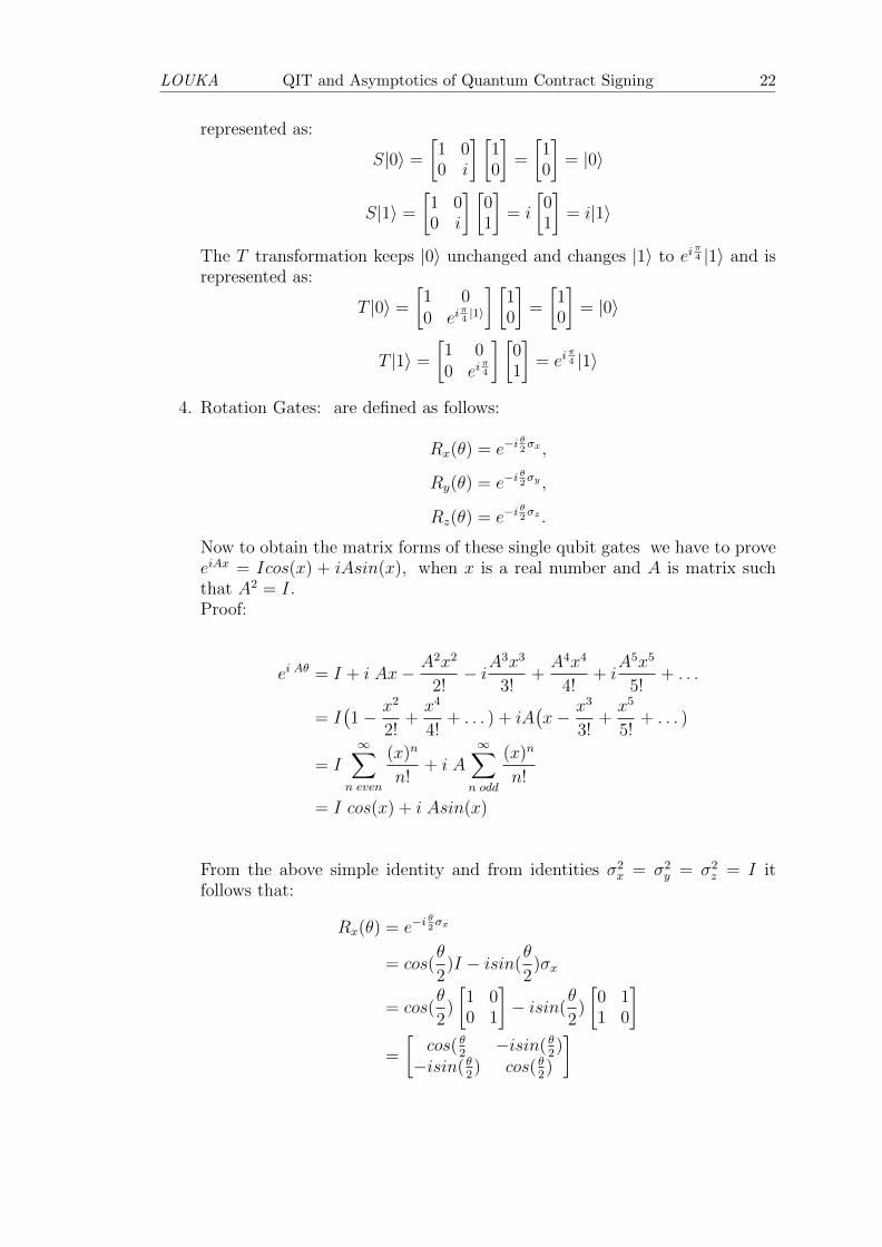
4. Rotation Gates: are defined as follows:
Rx(θ) = e−iθ2σx ,
Ry(θ) = e−iθ2σy ,
Rz(θ) = e−iθ2σz .
Now to obtain the matrix forms of these single qubit gates we have to proveeiAx = Icos(x) + iAsin(x), when x is a real number and A is matrix suchthat A2 = I.Proof:
ei Aθ = I + i Ax− A2x2
2!− iA
3x3
3!+A4x4
4!+ i
A5x5
5!+ . . .
= I(1− x2
2!+x4
4!+ . . . ) + iA
(x− x3
3!+x5
5!+ . . . )
= I∞∑
n even
(x)n
n!+ i A
∞∑n odd
(x)n
n!
= I cos(x) + i Asin(x)
From the above simple identity and from identities σ2x = σ2
y = σ2z = I it
follows that:
Rx(θ) = e−iθ2σx
= cos(θ
2)I − isin(
θ
2)σx
= cos(θ
2)
[1 00 1
]− isin(
θ
2)
[0 11 0
]=
[cos( θ
2−isin( θ
2)
−isin( θ2) cos( θ
2)
]

LOUKA QIT and Asymptotics of Quantum Contract Signing 23
Ry(θ) = e−iθ2σy
= cos(θ
2)I − isin(
θ
2)σy
= cos(θ
2)
[1 00 1
]− isin(
θ
2)
[0 −ii 0
]=
[cos( θ
2−sin( θ
2)
sin( θ2) cos( θ
2)
]
Rz(θ) = e−iθ2σz
= cos(θ
2)I − isin(
θ
2)σz
= cos(θ
2)
[1 00 1
]− isin(
θ
2)
[1 00 1
]=
[e−i
θ2 0
0 eiθ2
]
5. Square root of-Not: One of the simplest non classical gates1
V =√NOT =
[0 11 0
] 12
=(1 + i)
2
[1 −i−i 1
]=
[1+i
21−i
21−i
21+i
2
]it is very easy to check that V.V = NOT :[
1+i2
1−i2
1−i2
1+i2
] [1+i
21−i
21−i
21+i
2
]=
[0 11 0
]2.2.2 Two Qubit Gates
The general state of a two qubit system can be described as:
|ψ〉 = α00|00〉+ α01|01〉+ α10|10〉+ α11|11〉 =
α00
α01
α10
α11
The most important two qubit gates are the Controlled NOT gate or CNOT, Swapgate and Controlled-U gate
1. CNOT Gate: The first bit of a CNOT gate is called the control bit, and thesecond the target bit. The control bit does not change, while the target bitflips only when the control bit is 1, and it is works as following:
|00〉 → |00〉1 There are seven basic classical logic gates: AND, NOT, OR, XOR, NAND, NOR, and XNOR.

LOUKA QIT and Asymptotics of Quantum Contract Signing 24
|01〉 → |01〉
|10〉 → |11〉
|11〉 → |10〉
it is represent in bra-ket notation as follows:
CNOT = |0〉〈0| ⊗ I + |1〉〈1| ⊗ σxThus the matrix representation for this gate is:
CNOT =
1 0 0 00 1 0 00 0 0 10 0 1 0
2. Controlled-U Gate: can be implemented using single qubit gates (e.g., U
= σx, σy, σz, H, S, V . . . ) and CNOT, and it is works as follows:
|00〉 → |00〉|01〉 → |01〉|10〉 → |1〉 ⊗ U |0〉|11〉 → |1〉 ⊗ U |1〉
and it is represnt by bra-ket as follows:
Controlled-U Gate = |0〉〈0| ⊗ I + |1〉〈1| ⊗ U
Thus the matrix representation for this gate is:
Controlled-U =
[I OO U
],
where I is identity matrix, O =
[0 00 0
]and U is any quantum gate with
2× 2 unitary matrix. For instance (U = X, Y, Z,H, S, · · · ). We can see thatCNOT gate is a special case of controlled U where U = X
3. Swap Gate: the swap gate swaps the state of two qubits; thus it maps|mn〉 → |nm〉 (i.,e.|00〉 → |00〉, |01〉 → |10〉, |10〉 → |01〉 and |11〉 → |11〉)and it can represented by the matrix:
SWAP =
1 0 0 00 0 1 00 1 0 00 0 0 1
2.2.3 Three Qubit Gates
The Toffoli and Fredkin gates are an examples of three qubit gates

LOUKA QIT and Asymptotics of Quantum Contract Signing 25
1. Toffoli gate (Controlled-Controlled-NOT): The Toffoli gate takes the state|abc〉 to the state |abc′〉 as follows:
|000〉 → |000〉;
|001〉 → |001〉;
|010〉 → |010〉;
|011〉 → |011〉;
|100〉 → |100〉;
|101〉 → |101〉;
|110〉 → |111〉;
|111〉 → |110〉.
It can be understood as a gate that flips the third input bit if and only if thefirst two input bits are both 1.Now we can representing Toffoli gate as:
Toffoli =
1 0 0 0 0 0 0 00 1 0 0 0 0 0 00 0 1 0 0 0 0 00 0 0 1 0 0 0 00 0 0 0 1 0 0 00 0 0 0 0 1 0 00 0 0 0 0 0 0 10 0 0 0 0 0 1 0
2. Fredkin gate: also known as Controlled-SWAP swaps the last two bits if and
only if the first bit is |1〉, as follows:
|000〉 → |000〉;
|001〉 → |001〉;
|010〉 → |010〉;
|011〉 → |011〉;
|100〉 → |100〉;
|101〉 → |110〉;
|110〉 → |101〉;
|111〉 → |111〉.

LOUKA QIT and Asymptotics of Quantum Contract Signing 26
and it can represented by the matrix:
Fredkin =
1 0 0 0 0 0 0 00 1 0 0 0 0 0 00 0 1 0 0 0 0 00 0 0 1 0 0 0 00 0 0 0 1 0 0 00 0 0 0 0 0 1 00 0 0 0 0 1 0 00 0 0 0 0 0 0 1
2.3 Universal Quantum Gates
We know in classical computers that, for instance, the gates NAND and NOR areuniversal, see [51, p. 57,p. 92], because we can build any logic gate using onlyNAND or NOR gates.
Example 2.1. A NOT gate can be obtained using a NAND gate:
[(A|A) has the same values as ¬A]
Table 2.1: NOT in terms of NANDA A A|A ¬A0 0 1 1
1 1 0 0
Example 2.2. An AND gate can be obtained using only NAND gate:
[A ∧B ≡ (A|B)|(A|B)]
Table 2.2: AND in terms of NANDA A A|B A|B (A|B)|(A|B)
0 0 1 0 0
0 1 1 0 0
1 1 1 0 0
1 0 0 1 1
In quantum computation, a similar situation occurs. The set of gates such thatany unitary operator can be expressed by a quantum circuit using only the gatesfrom that set is called a universal set of quantum gates. For example, one suchuniversal set, as showed by Barenco, consists of the following two qubit gates, see[12, pp. 108-110],[31, pp. 67-71],[13]:
A(φ, α, θ) =
1 0 0 00 1 0 00 0 eiαcos(θ) −ie(α+φ)sin(θ)0 0 −ie(α−φ)sin(θ) eiαcos(θ)

LOUKA QIT and Asymptotics of Quantum Contract Signing 27
If we set θ = π/2, φ = 0 and α = π/2 the Barence gate operates as a CNOTgate:
CNOT =
1 0 0 00 1 0 00 0 0 10 0 1 0
By setting θ = π/2, φ = 3π/2 and α = π/2 the Barence gate operates as acontrolled-Y gate
(in short C(Y)
):
C(Y ) =
1 0 0 00 1 0 00 0 0 −i0 0 i 0
By setting α = φ = 0 and θ = π/2 the Barence gate operates as an Identitymatrix:
I =
1 0 0 00 1 0 00 0 1 00 0 0 1
2.4 Quantum Algorithms
Quantum algorithms can be modelled by a unitary transformation of n-qubit stateusing quantum gates. Such transformation is always reversible, i.e. by playingsteps of the algorithm in reverse, we get the original state.
However, the last step of a quantum algorithm is quantum measurement. Thisstep is not reversible, and gives one state of the measured basis with correspondingprobability.
Because of the measurement step, all quantum algorithms are in essence proba-bilistic. It is however possible to emulate any classical computation on a quantumcomputer.
In the following section we will explain structure of two of the most importantquantum algorithms.
2.4.1 Shor’s Algorithm
In 1994 Peter Shor published Shor’s algorithm (see [45, pg. 105-110],[21, pg. 4-8]) for factoring big number N but the clasical part was known before. It takespolynomial time in log N , specifically O
((log N)3
). Classically, best known prime
factorization algorithms take asymptically Cexp[(log N)1/3](log N)2/3 steps.
He shows (in principle), that quantum computer is capable of factoring very largenumber in polynomial time (polynomial in the number of digits of the number).

LOUKA QIT and Asymptotics of Quantum Contract Signing 28
To understand the Shor’s algorithm (and RSA algorithm in the next chapter), weshall need several mathematical ingredients from basic mathematics and numbertheory, see paper [37, pp. 159-186]:
Definition 2.1. (Division Algorithm for Integers). Let a, b ∈ Z with b > 1. Thenthere exist unique q, r ∈ Z such that a = bq + r, 0 ≤ r < b. If r = 0, we say that bdivides a and denote this by b|a.
Definition 2.2. (Greatest common divisor). Let a, b ∈ Z. A positive integer d isthe greatest common divisor of a and b if
1. d|a and d|b,
2. if c is a positive integer satisfying c|a and c|b, then c|d.
The greatest common divisor of a and b is denoted by gcd(a, b).
Theorem 1. (Euclidean Algorithm) To compute the greatest common divisorof two numbers a and b, let r−1 = a, let r0 = b, and compute successive quotientsand remainders:
ri−1 = qi+1 × ri + ri+1
for i = 0, 1, 2, . . . until some remainder rn+1 is 0. The last nonzero remainder rnis then the greatest common divisor of a and b.
Primality and coprimality play a central role in the arithmetic of the RSA cryp-tosystem.
Definition 2.3. (Prime Integer) An integer p ≥ 2 is said to be prime if its onlypositive divisors are 1 and p.
Definition 2.4. (Relatively Prime or Coprime Integers) Two integers a and b aresaid to be relatively prime or coprime if gcd(a, b) = 1.
Definition 2.5. (RSA Modulus) Let p and q be large prime numbers such thatp 6=q. The product N = pq is called an RSA modulus.
Definition 2.6. (Modular Arithmetic) a ≡ b(modc)↔ a = b+kc for some integerk.
Example 2.3. 21 ≡ 1(mod 4) because 21 = 1 + 5(4)52 ≡ 3(mod 11) because 25 = 3 + 2(11)
2.4.1.1 General Steps of Shor’s Algorithm
1. A reduction, which can be done on classical computer, of the factoring prob-lem to the problem order finding.
2. A quantum algorithm to solve the problem order fining.
Classical Part : Reduction to Order Finding
1. scale integer a such that 1 < a < N .
2. compute z = gcd(a,N). This may be done by Euclidean algorithm .

LOUKA QIT and Asymptotics of Quantum Contract Signing 29
3. if z = gcd(a,N) 6= 1 then there is a nontrivial factor of N, so we aredone.
4. otherwise, use the period-finding subroutine (below) to find r , the periodof the following function:
f(x) = axmodN
i.e. r is the smallest integare such that ar = 1modN .
5. if r is odd go back to step 1.
6. otherwise, z = max{gcd(N, ar − 1), gcd(N, ar + 1)}.7. if z = 1 go back to step 1.
8. The factors of N are z = gcd(N, ar/2− 1) and gcd(N, ar/2 + 1). we aredone.
Example 2.4. Let us factor N = 15 using classical order finding.
• Choose a < 15 such that gcd(a, 15) = 1 : a = 2.
• Calculate f(x) = axmod15 and find order r of f(x)
x ax 2xmod15
x ax 2xmod151 21 = 2 2mod15 = 22 22 = 4 4mod15 = 43 23 = 8 8mod15 = 82 24 = 16 16mod15 = 1
Therefore r = 4
• Note here in this example r is even:
• The factors of 15 are z = gcd(15, 22 − 1) = 3 and gcd(15, 22 + 1) = 5
3× 5 = 15
Before we start with the Quantum part we will explain important things weneed in order to understand this part:
Quantum Fourier Transform (QFT): This is the backbone of the Shor’salgorithm.In this section we will first explain what the (QFT) and discrete Fouriertransform (DFT) mean. This part is based on the paper [32, pp. 211-212].The (DFT) transforms an input vector of complex numbers x1, x2, . . . , xn−1
into an output vector of complex numbers y1, y2, . . . , yn−1 expressed as:
yk =1√q
q−1∑j=0
xje2πijk/q
The QFT does the same transformation as the DFT, except it operates lin-early on quantum states |0〉, . . . , |q − 1〉, which form an orthonormal basis.

LOUKA QIT and Asymptotics of Quantum Contract Signing 30
The QFT is
j −→ 1√q
q−1∑k=0
e2πijk/q|k〉
Assume that q is power of 2 (q = 2n) then:
j −→ 1√2n
2n−1∑k=0
e2πijk/2n|k〉
Binary expression:
j = j020 + j121 + j222 + · · ·+ jn−12n−1
k = k020 + k121 + k222 + · · ·+ kn−12n−1
The term jk/2n in (2) can be written as:
jk
2n=
1
2n(j020 + j121 + j222 + · · ·+ jn−12n−1)
× (k020 + k121 + k222 + · · ·+ kn−12n−1)
=1
2n[k0(j020 + j121 + j222 + · · ·+ jn−12n−1)
+ k121(j020 + j121 + j222 + · · ·+ jn−12n−1)
+ · · ·+ kn−12n−1(j020 + j121 + j222 + · · ·+ jn−12n−1)]
=1
2n[k0(j020 + j121 + j222 + · · ·+ jn−12n−1)]
+ k1[j021 + j122 + j223 + · · ·+ jn−12n]
+ · · ·+ kn−1[j02n−1]
= k0
( j0
2n+
j1
2n−1+ · · ·+ jn−1
2) + k1
( j0
2n−1+
j1
2n−2
+ · · ·+ jn−1
2
)+ · · ·+ kn−1
j0
2
Any binary fraction j can be written as follows: j = jl2
+ jl+1
4+· · ·+ jm
2m−l+1 and
we can use notation [jljl+1jl+2 · · · jm], for instance: [0.j0] → j02, [0.j0j1] →
j04
+ j12
, with this notation, we can write j −→ 1√2n
2n−1∑k=0
e2πijk/2n|k〉 as:
1√2n
2n−1∑k=0
e2π[0.jn]k1|k1〉 ⊗ e2π[0.jn−1jn]k2|k2〉 ⊗ · · · ⊗ e2π[0.j1j2···jn]kn|kn〉
Where the state |k〉 : (k ∈ [0, 1]), Then the last equation is equal to
1√2n
(|0〉+ e2π[0.jn]|1〉
)⊗(|0〉+ e2π[0.jn−1jn]|1〉
)⊗ · · · ⊗
(|0〉+ e2π[0.j1j2···jn]|1〉
Quantum Part:

LOUKA QIT and Asymptotics of Quantum Contract Signing 31
Figure 2.1: The QFT circuit consists of Hadamard gates and unitary Phase transformgates
H R1 Rn-2 Rn-1
H Rn-2 Rn-3
H R1
H
|jn-1 >
|jn-2>
|j1>
|j0>
|0>+e2pi I [j0… j
n-1] |1>
|0>+e2pi I [j
0… j
n-2] |1>
|0>+e2pi I [j0… j
1] |1>
|0>+e2pi I [j0
] |1>
I get this paragraph from paper [38, pg. 194-197]. To factorN , find 2 log2N <n < 2 log2
√2N : q = 2n and choose x such that 1 < x < N−1, gcd(x,N) = 1
Step 0: Initialize state.|ψ0〉 = |00 . . . 0〉⊗n|00 . . . 0〉⊗l
Step 1: Application of H⊗n on first register yielding
|ψ1〉 =1√2n
2n−1∑k=0
|k〉|0〉
Step 2: Apply modular exponentiation: f(k) = xkmodN on second registeryielding
|ψ2〉 =1√2n
2n−1∑k=0
|k, f(k)〉
Step 3: Measure the second register. Note that the second register will be in abase state where e is some power of xmodN and all powers of xmodN areequally likely to be observed
|ψ3〉 =1√m
∑k∈K
|k, e〉,
K = {k : xk modN = e} and m = |K| is the number of elements in K
That is K = {k0, k0 +r, k0 +2r, . . . , k0 +(m−1)r}, k0 is first element in K.
|ψ3〉 =1√m
m−1∑j=0
|k0 + jr, e〉

LOUKA QIT and Asymptotics of Quantum Contract Signing 32
Step 4: Apply the Quantum Fourier Transform (QFT) to the first register thistransforms the state from
|ψ3〉 =1√m
m−1∑j=0
|k0 + jr, e〉 to |ψ4〉,
|ψ4〉 =1√qm
q−1∑c=0
m−1∑j=0
e2πic(k0+jrq
)|k, e〉
=
q−1∑c=0
e2πick0q
√qm
m−1∑j=0
e2πicjrq |k, e〉
=
q−1∑c=0
e2πick0q
√qm
m−1∑j=0
ζj|k, e〉 where ζ = e2πicrq
Step 5: Measure register 1. Note that register 1 has probability to be in state |c〉
pr(c) =1
qm
m−1∑j=0
|ζj|2 where ζ = e2πicrq
This is returns some numbers
I cq≈ j
rsuch that pr(c) is very high
But to determine the order r we need to estimate j, where is j equal to aninteger number.
Step 6: We can calculate the order of N by computing the convergent of con-tinuous fraction expansion of c
qand retuning the closest such fraction of O
r
where O is an integer
I continued fraction expansion:
c
q= a0 +
1
a1 +1
a2 +1
a3 +1
a4 + . . .

LOUKA QIT and Asymptotics of Quantum Contract Signing 33
I Convergent of Continued Fraction:The n-th convergent of the sequence ai is defined to be:
pnqn
= [a0, a1, a2, . . . , an]
p0
q0
≈ a0
1= a0
p1
q1
≈ a0 +1
a1
p2
q2
≈ a0 +1
a1 + 1a2
=a2p1 + p0
a2q1 + q0
=a2(a1a0 + 1)
a2a1 + 1
p3
q3
≈ a0 +1
a1 + 1a2+ 1
a3
=a3p2 + p1
a3q2 + q1
=a3(a2(a1a0 + 1)) + (a1a0 + 1)
a3(a2a1 + 1) + a1
pnqn≈ a0 +
1
a1 +1
a2 +1
a3 +1
. . . + 1an
=anpn−1 + pn−1
anqn−1 + qn−1
Then one considers pnqn
= [a1, a2, a3, . . . , an] converging to cq
(pnqn
is a sequence of
continued fractions of cq); we will use notation j
r1for values of continued fractions
for cq. If r1 < N try small multiples of r1 as possible values of r:
r1, 2r1, 3r1, . . . ,⌊log (N1+ε)
⌋r1,
(this was suggested by Odlyzko), and check when xr mod N = 1.Finaly find gcd(y+1, N), gcd(y−1, N) = factoring of N where y = xr/2 mod N .
Example 2.5. Factoring N = 21 using Shor’s algorithm.
I We have l = log2N = 4.3 ≈ 4, n = 2 log2N = 8.7 ≈ 9, 2 log2
√2N = 9.7 such
that 8.7 < 9 < 9.7
I Choose x = 8 such that 1 < 8 < 21 and gcd(8, 21) = 1
Step 0: Initialize state.
|ψ0〉 = |00 . . . 0〉⊗n|00 . . . 0〉⊗l = |00 . . . 0〉⊗9|00 . . . 0〉⊗4
Step 1: Application of H⊗n on first register yielding
|ψ1〉 =1√512
511∑k=0
|k, 0〉 =1
512
(|0, 0〉+|1, 0〉|2, 0〉+|3, 0〉+|4, 0〉+· · ·+|511, 0〉
)step 2: Apply modular exponentiation: f(k) = xkmodN
|ψ2〉 =1√512
511∑k=0
|k, f(k)〉 =1
512
(|0, 1〉+ |1, 8〉+ |2, 1〉+ |3, 8〉+ · · ·+ |511, 8〉
)

LOUKA QIT and Asymptotics of Quantum Contract Signing 34
Step 3: Observe register 2; Suppose we observe 8; as a power of xkmodN
|ψ3〉 =1√256
(|3, 8〉+ |5, 8〉+ |7, 8〉+ |9, 8〉+ |11, 8〉+ · · ·+ |511, 8〉
)Step 4: Apply Quantum Fourier Transform on |ψ3〉 to obtain
|ψ4〉 =1
131072
511∑c=0
e2πic( 255∑j=0
ζj|c〉)
where ζ = e2πi.cr
512
Step 5: Measure register 1
pr(c) =1
131072|
255∑j=0
ζj|2 where ζ = e2πi.cr
512 , c ∈ [0, 511] and j ∈ [0, 255]
Assume that we obtain |256〉
pr(256) =1
131072|
255∑j=0
e2πij|2 = 0.5
where c2n
= 12
= 0 + 12
which can be written in continued fraction form as [0, 2]. Sor1 = 2. Now we check xr1 mod N and we find that xr1 mod N = 82 mod 21 = 1.Thus the required period is 2 where y = x
r2 mod N = 8 mod 21 = 8.
Then the factor of N = 21 are: gcd(y ± 1, 21) = gcd(8± 1, 21) = 3 and 7.
2.4.2 Grover’s Algorithm
Grover algorithm was invented by Lov Grover in 1996. The main goal for Grover’salgorithm is to search an unsorted database more efficiently, with N entries re-quiring O(
√N) time (the best classical algorithm can do this in time proportional
to N).
A simple example is to find a desired file index among N = 2n files. The importantthings to understand for Grover algorithm are: Oracle function (black box) andquantum Oracle, see [49], [26] .
I Oracle (black box) that can recognize the solution, whose internal working isrepresented by a binary function
f : {0, 1}n −→ {0, 1}
Defined by:
f(x) =
{1 if x is a solution
0 otherwise
I Quantum Oracle: in this case, we are given a unitary operation |x〉 Uw→ (−1)f(x)|x〉as a black box operation.
LOUKA QIT and Asymptotics of Quantum Contract Signing 35
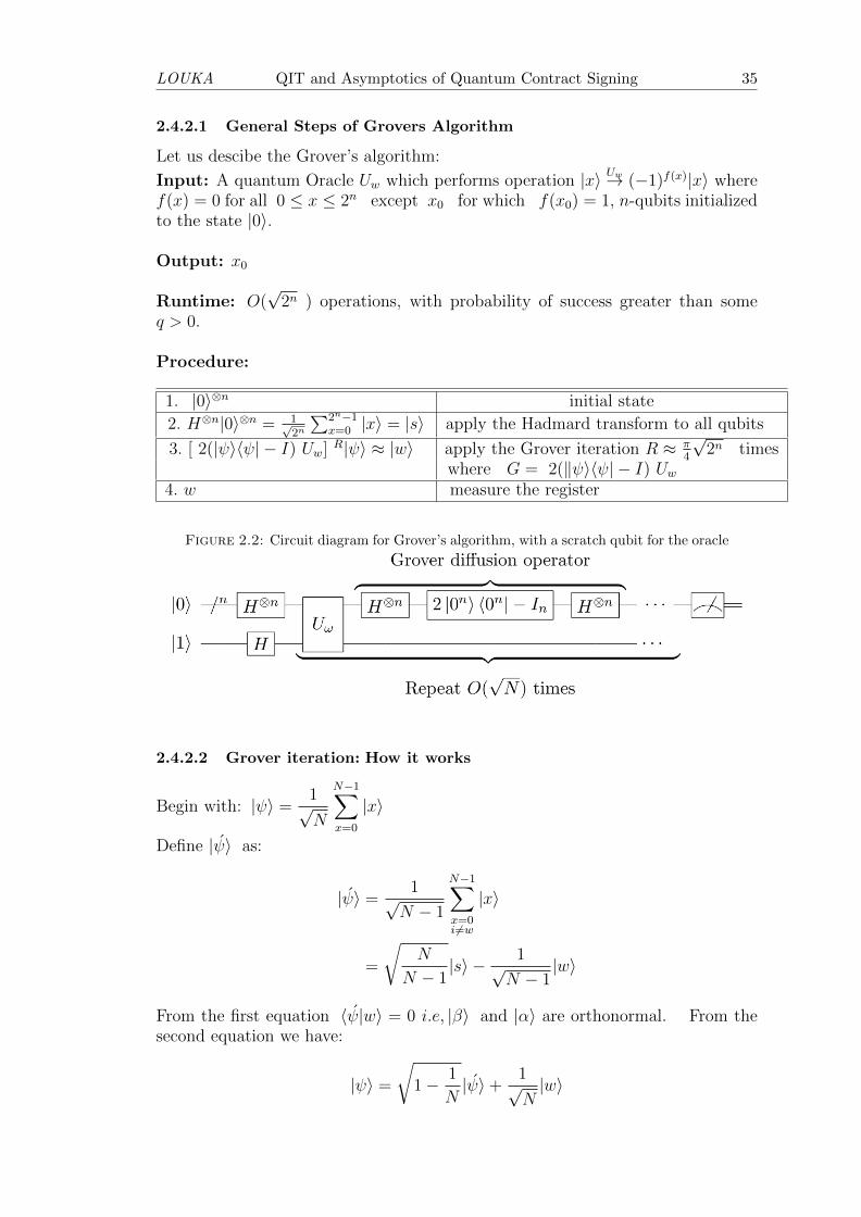
2.4.2.1 General Steps of Grovers Algorithm
Let us descibe the Grover’s algorithm:
Input: A quantum Oracle Uw which performs operation |x〉 Uw→ (−1)f(x)|x〉 wheref(x) = 0 for all 0 ≤ x ≤ 2n except x0 for which f(x0) = 1, n-qubits initializedto the state |0〉.
Output: x0
Runtime: O(√
2n ) operations, with probability of success greater than someq > 0.
Procedure:
1. |0〉⊗n initial state
2. H⊗n|0〉⊗n = 1√2n
∑2n−1x=0 |x〉 = |s〉 apply the Hadmard transform to all qubits
3. [ 2(|ψ〉〈ψ| − I) Uw] R|ψ〉 ≈ |w〉 apply the Grover iteration R ≈ π4
√2n times
where G = 2(‖ψ〉〈ψ| − I) Uw4. w measure the register
Figure 2.2: Circuit diagram for Grover’s algorithm, with a scratch qubit for the oracle
2.4.2.2 Grover iteration: How it works
Begin with: |ψ〉 =1√N
N−1∑x=0
|x〉
Define |ψ〉 as:
|ψ〉 =1√
N − 1
N−1∑x=0i 6=w
|x〉
=
√N
N − 1|s〉 − 1√
N − 1|w〉
From the first equation 〈ψ|w〉 = 0 i.e, |β〉 and |α〉 are orthonormal. From thesecond equation we have:
|ψ〉 =
√1− 1
N|ψ〉+
1√N|w〉

LOUKA QIT and Asymptotics of Quantum Contract Signing 36
The state of the quantum computer at each step is:
Gk|ψ〉 = cos(2k + 1
2θ)|ψ〉+ sin(
2k + 1
2θ)|w〉
The value of θ is obtained substituting k for 0 in last equation ( Gk|s〉 ) andcomparing it with |ψ〉 equation:
θ = 2 arccos
√1− 1
N
The number of times k0 that G must be applied obeys the equation:
k0θ +θ
2=π
2
The number of steps required to find the desired element is:
k = round(π
4
√N) times
After applying G k times, the probability p of finding the desired elementafter a measurement is:
p = sin2(2k + 1
2θ)
Figure 2.3: Picture showing the geometric interpretation of the first iteration ofGrover’s algorithm. The state vector |s〉 is rotated towards the target vector |w〉 as
shown
Example 2.6. We consider a system consisting of N = 16 = 24 states, and thestate we are searching for, i0 = β, is represented by the bit string |1011〉.To describe this system, n = 4 qubits are required, represented as:|x〉 = |0000〉+ |0001〉+ |0010〉+ |0011〉+ |0100〉+ |0101〉+ |0110〉+ |0111〉+ |1000〉+|1001〉+ |1010〉+ |1011〉+ |1100〉+ |1101〉+ |1110〉+ |1111〉
Grover’s algorithm begins with a system initialized to 0: |0000〉and then apply the Hadamard transformation to obtain equal amplitudes associatedwith each state of 1√
N= 1√
16= 1
4and thus also equal probability of being in any of

LOUKA QIT and Asymptotics of Quantum Contract Signing 37
the 16 possible states:
H⊗4|0000〉 =1
4
15∑x=0
|x〉
The Grover iteration will be repeated k = π4
√N times. In our case k = π
4
√16 =
3.1415 which rounds to 3 iterations.Now, perform the diffusion transform [2|s〉〈s| − I]|x〉
[2|ψ〉〈ψ| − I]|x〉 = [2|ψ〉〈ψ| − I][|ψ〉 − 2
4|1011〉
= 2|ψ〉〈ψ|ψ〉 − |ψ〉 − 2(2
4)|ψ〉〈ψ|1011〉+
2
4|1011〉
Note that 16× 14
(14
). Additionally, we can use 〈ψ|1011〉 = 〈1011|s〉 = 1
4, so
= |ψ〉 − 1
4|ψ〉+
1
2|1011〉
=3
4|ψ〉+
1
2|1011〉
Substituting |ψ〉 = 14
∑15x=0 |x〉 gives:
=3
4
[1
4
15∑x=0
|x〉]
+1
2|1011〉
=3
16
15∑x=0x 6=11
|x〉+[ 3
16|1011〉+
1
2|1011〉
]
=⇒ |x1〉 =3
16
15∑x=0x 6=11
|x〉+11
16|1011〉
This is completes the first iteration.
We apply the same two transformations in the second iteration (Oracle) in Groveralgorithm, which gives:
|x2〉 =3
16
15∑x=0x 6=11
|x〉 − 11
16|1011〉
=3
16
15∑x=0x 6=11
|x〉+[− 11
16|1011〉 − 3
16|1011〉
]

LOUKA QIT and Asymptotics of Quantum Contract Signing 38
After the Oracle query, and after applying the diffusion transform:
[2|ψ〉〈ψ| − I][3
4|ψ〉 − 7
8|1011〉] = 2
(3
4
)|ψ〉〈ψ|ψ〉 − 3
4|ψ〉 − 2
(7
8
)|ψ〉〈ψ|1011〉
=3
2|ψ〉 − 3
4|ψ〉 − 7
4|ψ〉(1
4
)+
7
8|1011〉
=5
16|ψ〉+
7
8|1011〉
=5
16
[1
4
15∑x=0x 6=11
|x〉+1
4|1011〉
]+
7
8|1011〉
=⇒ |x3〉 =5
64
15∑x=0x 6=11
|x〉+61
64|1011〉
We apply the same two transformations in the third iteration:
|x4〉 =5
64
15∑x=0x 6=11
|x〉 − 61
64|1011〉
After the oracle query, and after applying the diffusion transform:
[2|ψ〉〈ψ| − I][5
16|ψ〉 − 33
32|1011〉] = 2
( 5
16
)|ψ〉〈ψ|ψ〉 − 5
16|ψ〉
− 2(33
32
)|ψ〉〈ψ|1011〉+
33
32|1011〉
=5
8|ψ〉 − 5
16|ψ〉 − 33
16|ψ〉(1
4
)+
33
32|1011〉
=13
64|ψ〉+
33
32|1011〉
=13
256
15∑x=0
|x〉+33
32|1011〉
=13
256
15∑x=0x 6=11
|x〉+[33
32|1011〉+
13
256|1011〉
]
=⇒ |x5〉 =13
256
15∑x=0i 6=11
|x〉+251
256|1011〉
Longer format:|x5〉 = 13
256|0000〉 + 13
256|0001〉 + 13
256|0010〉 + 13
256|0011〉 + 13
256|0100〉 + 13
256|0101〉 +
13256|0110〉+ 13
256|0111〉+ 13
256|1000〉+ 13
256|1001〉+ 13
256|1010〉+ 251
6256|1011〉+ 13
256|1100〉+
13256|1101〉+ 13
256|1110〉+ 13
256|1111〉
Finally, to test Grover algorithm, we calculate the probability to find the state. Wefind :
p =∣∣∣251
256
∣∣∣2 =∣∣∣63001
65536
∣∣∣ = 96%

LOUKA QIT and Asymptotics of Quantum Contract Signing 39
The chance of getting the result |1011〉, is around 96%. and we observe that successprobability after each iteration four qubits is as follows:After the first iteration:
p =∣∣∣11
16
∣∣∣2 =∣∣∣121
256
∣∣∣ = 47%
After the second iteration:
p =∣∣∣61
64
∣∣∣2 =∣∣∣3721
4096
∣∣∣ = 90%
After the third iteration:
p =∣∣∣251
256
∣∣∣2 =∣∣∣63001
65536
∣∣∣ = 96%

Chapter 3
Cryptography and ContractSigning
3.1 Cryptography in General
When we want to keep information secret, we have two possible strategies: hidethe existence of the information, or make it unintelligible (cryptography), see [33,pg. 4] .
Definition 3.1. Cryptography is the study of mathematical techniques relatedto aspects of information security such as confidentiality, data integrity, entityauthentication, and data origin authentication.
The term cryptography comes from the two Greek words skrupto and graph, which,when literally translated, means ”secret writing”. Cryptography is the process ofdisguising the messages (information security) so that it can only be read by senderand receiver, in other words enabling sender and receiver to mask confidential mes-sages and to make tranmitted data illegible to any unauthorized third party, (see[42]).
The branch of mathematics encompassing both cryptography and cryptanalysis(decrypting of information or breaking the cryptographic designs) is cryptology .
cryptology = cryptography + cryptanalysis
A system to encrypt and decrypt information is known as cryptosystem.
Definition 3.2. Cryptosystem is a quintuple (P ;C;K;E ;D) such that:
1. P ,C, and K are finite sets, where
• P is the plain text space or clear text space,
• C is the cypher text space, and
• K is the key space.
Elements of P are referred to as plain text, and elements of C are referred toas cypher text. A message is a string of plain text symbols.
2. E = {Ek|k ∈ K} is a family of functions Ek : P → C that are used forencryption, and D = {Dk|k ∈ K} is a family of functions Dk : C → P thatare used for decryption.
40

LOUKA QIT and Asymptotics of Quantum Contract Signing 41
3. For each key e ∈ K there exists a key d ∈ K such that for each p ∈ P :
Dd(Ee(p)) = p
A cryptosystem is called symmetric if d = e (the same key is used to encrypt anddecrypt information), or if d can at least be easily computed from e.A cryptosystem is called asymmetric if d 6= e (one key is used to encrypt and adifferent key to decrypt) and it is computationally infeasible in practice to computed from e. Here, d is the private key and e is the public key. Public key is knownboth to the sender and to the adversary, but only the receiver can decrypt cipherbecause he or she knows the secret private key, and the steps as follows:
1. The sender converts the message into ciphertext using an encryption system.private key + plaintext −→ ciphertext
2. The receiver converts the ciphertext back into plaintext using a correspondingsystem.private key + ciphertext −→ plaintext
3.1.1 RSA Algorithm
The RSA algorithm was first published in 1977 by group of three scientists, namelyRon Rivest, Adi Shamir and Len Adleman. It is a form of asymmetric cryptogra-phy and is used to encrypt and decrypt in message communication for making thecommunication secure where one user (part) uses public key and other user usessecret (private key), see [2, pp. 48-50] .
In order to understand RSA encryption we need the Euclidean Algorithm (The-orem 1), the method of successive squaring, Fermat’s Little Theorem and theChinese Remainder Theorem, see [14].
Definition 3.3. (Euler’s Phi Function) Let n be a positive integer. Eulers PhiFunction, denoted φ(n), is the number of positive integers ≤ n which are relativelyprime to n, computed as:
φ(n) = n∏p|n
(1− 1
p)
For example φ(6) = 6 × (1 − 12) × (1 − 1
3) = 2 because in the set {1, 2, 3, 4, 5, 6}
only two numbers 1 and 5 are coprime to 6.
Lemma 1. If n is prime, then φ(n) = n− 1.
Proof. Let n be a prime number. Since n is prime, 1, 2, 3, 4, ..., n− 1 are relativelyprime to n. Therefore, φ(n) = n− 1.
If p and q are prime, then φ(pq) = φ(p)φ(q) = (p− 1)(q − 1).
Theorem 2. (Euler’s Theorem) If a and n are two relatively prime positiveintegers, then
aφ(n) ≡ 1(mod n).

LOUKA QIT and Asymptotics of Quantum Contract Signing 42
For instance, when p = 3 and q = 5 then
a8 = 1(mod 15)
for any integer a that has no common divisior with pq; we verify that
28 = 1(mod 15)
48 = 1(mod 15)
78 = 1(mod 15)
The particular case in which n is a prime number p, Euler’s theorem is calledFermat’s Little Theorem.We use the following Lemma to prove the Fermat’s Little Theorem:
Lemma 2. For any prime p, we have
(x+ y)p = xp + yp mod(p).
Theorem 3. (Fermat’s Little Theorem) For any prime p and any positiveinteger a,
ap ≡ a(mod p)
Proof. There are several proofs using different techniques to prove the statementap ≡ a(mod p) but the most straightforward way to prove this theorem is byapplying the induction principle.The proof is by induction on a. When a = 1 is obviously true. ap = 1p = 1 = a so1p ≡ 1(mod p)Assume that kp ≡ k(mod p) (inductive hypothesis) and consider (k + 1)p. By theprevious lemma, we have (k+1)p ≡ kp+1p(mod p) and inductive hypothesis gives:
(k + 1)p ≡ (k + 1)(mod p)
By the principle of induction, it follows that ap ≡ a(mod p), for every positiveinteger a.
For instance, if a = 2 and p = 7, then we have, in fact, 27−1 = 26 = 64 = 1+9 ·7 ≡1(mod 7).
Theorem 4. (Chinese Remainder Theorem)(see [10][pp. 194–207] and [8][p .147])Let m1,m2, . . . ,mn be distinct positive integers such that gcd(mi,mj) = 1 if i 6= j.Then, for any integers a1, a2, . . . , an, consider the simultaneous congruences
x ≡ a1(mod m1)
x ≡ a2(mod m2)
x ≡ a3(mod m3)
...
x ≡ an(mod mn)
There exists an unique modulo solution of the system of simultaneous congruencesabove:
x = a1M1y1 + a2M2y2 + · · ·+ anMnyn(mod M)

LOUKA QIT and Asymptotics of Quantum Contract Signing 43
where M = m1m2 . . .mn, M1 =M
m1
, . . . ,Mn =M
mn
and M1y1 ≡ 1(mod m1),
. . . ,Mnyn ≡ 1(mod mn)
Example 3.1. Find solutions to
x ≡ 3(mod 5)
x ≡ 7(mod 8)
x ≡ 5(mod 7)
Solution:We have a1 = 3, a2 = 7, a2 = 7, a3 = 5, m1 = 5, m2 = 8, m3 = 7 and M =5 ∗ 8 ∗ 7 = 280
M1 =M
m1
=280
5= 56
M2 =M
m2
=280
8= 35
M3 =M
m3
=280
7= 40
we still need to find y1, y2 and y3, so we need to solve the equation
56 y1 ≡ 1(mod 5)
56 y2 ≡ 1(mod 8)
40 y3 ≡ 1(mod 7)
Therefore y1 = 1, y2 = 3 and y3 = 3Then
x =
≡1 mod 5︷ ︸︸ ︷(8 ∗ 7) ∗ 1 ∗ 3︸ ︷︷ ︸≡3 mod 5
+
≡1 mod 8︷ ︸︸ ︷(5 ∗ 7) ∗ 3 ∗ 7︸ ︷︷ ︸≡7 mod 8
+
≡1 mod 7︷ ︸︸ ︷(5 ∗ 8) ∗ 3 ∗ 5︸ ︷︷ ︸≡2 mod 7
The RSA algorithm involves three steps (see [2][pp. 15,16] and [41][pp. 165-168]):key generation, encryption and decryption:
3.1.1.1 Key Generation:
1. We begin by choosing two large prime numbers, p and q.
2. We compute n = p× q.
3. We compute the Euler’s function ϕ(n) = ϕ(p)ϕ(q) = (p− 1)(q − 1).
4. Next we choose a small number e such that gcd(e, ϕ(n)) = 1 and find d suchthat ed = 1 mod ϕ(n), in other words d = e−1 mod(ϕ(n)).
5. We now have two key values:The public key: (n, e)The private key: (n, d)

LOUKA QIT and Asymptotics of Quantum Contract Signing 44
3.1.1.2 Encryption and Decryption:
1. To encrypt a message m so it results in ciphertext c we use the following:
c = memod n (remember encryption is done with the public key)
2. To decrypt a message c so it results in plaintext c we use the following:
m = cdmod n (remember decryption is done with private key)
Theorem 5. (The correctness of the RSA algorithm). (see [22])Let m, c, n, e, d be plaintext, ciphertext, encryption exponent and modules respec-tively, then
c = memod n
m = cdmod n
So
cd = m mod n
Proof. Follows from Euler’s theorem:
aφ(n) ≡ 1(mod n)
since we have ed = 1 modφ(n) =⇒ ed = kφ(n) + 1 for some integer k, we canwrite
cd = (me)dmod n
= medmod n
= mkφ(n)+1mod n
= m.(mφ(n)kmod n
= m.1kmod n
= m mod n
So now that we know the theory behind how RSA encryption works, lets considerone example.
Example 3.2. Take two large primes: p=37, q=23The product of p and q is n, in our case:
n = p× q = 37× 23 = 851
The Euler’s phi function, φ(n) is calculated below:
ϕ(n) = ϕ(p)ϕ(q) = (p− 1)(q − 1) = 36× 22 = 792
Now we have to choose e = 5 such that e < n and gcd(e, ϕ(n)) = 1. We can use5, as 5 < 851 and gcd(5, 792) = 1. The pair (e, n) is our public key that is used

LOUKA QIT and Asymptotics of Quantum Contract Signing 45
to encrypt messages, so the private key key: (n, e) = (851, 5)We must find a number such that: ed = 1mod ϕ(n) using Euclid’s algorithm, weget d = 317. So the private key: (n, d) = (851, 317).Suppose the plaintext value m is 88 then,For encryption: sender wishes to send to receiver the message m, sender computesciphertext as c = memod n and sends it to receiver:Here we use the Chinese Remainder theorem, an easy way to solve memod n(Ciphertext)
c = memod n
= 885mod 851
= 103
For decryption:receiver gets the ciphertext from sender:
m = cdmod n
= 103317mod 851
= 88
reciver knows the message is 88.
3.2 Digital Signatures
One way, in which RSA algorithm (or public key cryptography) is used, is for digi-tal signatures. They provide an authentication mechanism that adds to a messagea code, a signature, which corresponds to a message, but can be linked to theauthor.
In a way, it is public key cryptography in reverse - it uses private key for encryp-tion, but public key for decryption.
Each digital signature requires three elements.
• Way to generate keys, at random. A private and a public key are generated.
• Way to sign a message, i.e. attach a small signature corresponding to eachgiven message and private key.
• Way to verify the signature, i.e. using a public key and signed message,checks signature’s authenticity.
Example 3.3. Consider RSA protocol, but in reverse, i.e. such that key forencoding e is private, and key for decoding d is public. Then a signature would becomputed as
s = me (mod N),
and can be checked using d by comparing sd (mod N) and m.

LOUKA QIT and Asymptotics of Quantum Contract Signing 46
The signer sends some message, M , and appends his signature s, using short-ened version of message, m = h(M), computed according to some publicly knownfunction h, usually a function which is easy to compute but difficult to reverse, likeso called hash functions.
3.3 Quantum Cryptography and Quantum Key Distribu-tion
Quantum mechanics has some natural advantages for cryptography. For exam-ple, random numbers are generated by measurements, and there is no need forpseudorandom generators. This was noted in 1984. by Charles Bennett and GillesBrassard (see [47]), who proposed the first quantum cryptography protocol, knownas BB84.
This is a protocol for distribution of keys between two parties, Alice and Bob.The key is a n-bit sequence k. The message m is transformed to ciphertext cby bitwise addition, c = m + k (mod 2), and then the plaintext is recovered asm = p = c+ k (mod 2) by bitwise addition of key bits.
To distribute the secret key between Alice and Bob, in BB84 EPR states are used.To protect against the third party eavesdropping, a N pairs of entangled qubitsare used, where N > n. Each qubit is shared as an EPR state
|ψ+〉 =1√2
(|0〉1|1〉2 + |1〉1|0〉2
)=
1√2
(|+〉1|−〉2 + |−〉1|+〉2
)Where {|+〉, |−〉} will be the the ”reject basis”, {|0〉, |1〉} will be the the ”acceptbasis”
|+〉 =1√2
(|0〉+ |1〉), |−〉 =1√2
(|0〉 − |1〉), |0〉 =
[10
]and |1〉 =
[01
]The accept observable
A = 1.|1〉〈1|+ 0.|0〉〈0|
and the reject observable
R = 1.|+〉〈+|+ 0.|−〉〈−|
To generate a key, Alice chooses for each qubit either basis A or basis R tomeasure, and announces her choice publicly. Then Bob measures the same basison his corresponding qubits, and gets to know results that Alice got. Out of themeasured N qubits, randomly and publicly chosen n are used to get a secret sharedkey, and the remaining N −n are compared, again publicly. If they do not match,that is used as evidence of eavesdropping, and in that case everything is repeated.The proof of security of BB84 was obtained much later, see for instance paper [47].

LOUKA QIT and Asymptotics of Quantum Contract Signing 47
3.4 Contract Signing
Contract signing is a legal process, in which two parties (Alice and Bob) make abinding agreement. In law, it is defined in the following way:
Definition 3.4. Contract is a legally binding agreement made between two ormore parties who intend it to have legal effect and for which the law will providea remedy in the event of breach (see [19, pp. 3-16],[11, pp. 194-198]) .
The agreement can be formal, informal, written, oral or just plain understood.Some contracts are required to be in writing in order to be enforced. Legal termi-nology distinguishes offeror the party who makes an offer to enter in to a contract,and offeree the party to whom an offer to inter into a contract is made ,see [27,p. 375] .The necessary essential elements to form a binding contract are usually describedas:
1. An offer: is a proposal by one party (the offeror) to do or to give somethingand accepted by another party (the offeree).
2. An acceptance: To binding contract , there must be an acceptance of theoffer and it is done by compliance with the terms of the offer by the partyreceiving the offer (offeree). Both of them (offer and acceptance) are called”mutual assent” means there must meeting of minds.
The objective of the contract must be for a legal purpose. For example, acontract for illegal distribution of weapons is not a binding contract becausethe purpose for which it exists is not legal. if the parties violate the law.thecontract will deemed to be ”void” .
3. Consideration, i.e. something of value offered by offeror and accepted byofferee.
4. Competent Parties:meaning the parties who are legally qualified (that is, have the capacity) tomake a binding contractual agreement, see [9, pp. 353-356] .
If the contract complies with all essential elements, it is a valid contract, if the hasno legal effect at all then the contract is a void, see [15, p. 191].
Traditionally, paper-based contracts are signed by the transacting parties whoneed to be present at the same place and at the same time. Each party signs acopy of the contract and exchange signed papers, so that every party gets a copyof the signed contract.
When parties involved are physically far apart, alternative in this case signing anelectronic/digital signature contract. However, that poses a problem: one partycan get commitment from other party (a copy of the contract with her/his signa-ture on it) without committing himself (Cheater). The solution to this problemis to get a fair and viable contract signing protocol by involving a trusted thirdparty (TTP), which we will call Trent, to which both signers always send theirsignatures directly to it, see [29, p. 367].

LOUKA QIT and Asymptotics of Quantum Contract Signing 48
Definition 3.5. Fair protocol means that either both parties get each others’commitment or none gets.
An unfair protocol is one in which one party has proof of commitment from theother, but does not commit itself. Thus, for instance in stock market, one partymay want to buy futures or options, without commiting to the contract if the eventson the maket do not go to its advantage. Naturally, this is a highly undesirablesituation.
Definition 3.6. Viable protocol is one where, if both parties behave honestly, theywill both get each others’ commitments.
It can be shown that it is impossible to design a fair and viable contract signingprotocol, without involving the trusted party (i.e. Alice and Bob have to rely onTrent).However, it is desirable to involve Trent (i.e. a trusted third party) as little aspossible.
Definition 3.7. Optimistic protocols are protocols in which the third trusted partyin involved only when one party is cheating or the communication is interrupted.
In optimistic protocols, Alice and Bob exchange messages, so that in the end bothparties will end up with signed contract. However, if there is a disruption or ev-idence of cheating, the parties have an option to invoke Trent, who would thenbind the contract, assuring fairness.
Some protocols are only probabilisticaly fair, i.e. there is a small probability ofadvantage to one party. Such protocols have been designed using clasicall cryp-tography, which are both optimistic and probabilisticaly fair.
In classical cryptography, contract signing relies on digital signatures. However,using peculiarities of quantum mechanics, it is possible to design quantum con-tract signing protocols which do not rely on signed messages, see [39].

Chapter 4
Asymptotics of QuantumContract Signing
4.1 Paunkovic-Bouda-Mateus Protocol
The idea of quantum contract signing is to use a pair of non-commuting observ-ables (quantum complementarity), and inherent properties of quantum mechanics,to achieve a probabilistically fair, viable and optimistic protocol, without relianceon the digital signatures.
In [39], the following protocol is proposed for that purpose. Trent, a trusted thirdparty, sends to Alice and Bob in initialisation phase, N qubits each, and classicaldata about the qubits received by the other party. In exchange phase, Alice andBob make measurements of their choice on their qubits, and send the results tothe other party in alternating turns. This phase does not involve Trent (protocolis optimistic). However, if the exchange is interrupted or there is evidence ofcheating, they have an option to invoke Trent again. In this case binding phaseoccurs. They present to Trent their results of measurements and claims aboutwhich observables they measured. Trent then decides if the contract is a void,or if it is bound by the presented results. The idea is, that the party which washonest, has a way to enforce the contract (i.e. bind it) or reject it, the moment itnotices a problem (i.e. evidence of cheating by the other party).Let
|+〉 =1√2
(|0〉+ |1〉)
and
|−〉 =1√2
(|0〉 − |1〉)
Thus, {|+〉, |−〉} is an alternative orthonormal qubit frame. We will call this framethe ”reject basis”, while {|0〉, |1〉} will be the ”accept basis”. Define
A = 1 · |1〉〈1|+ 0 · |0〉〈0|R = 1 · |+〉〈+|+ 0 · |−〉〈−|
to be the corresponding accept and reject observables.
49

LOUKA QIT and Asymptotics of Quantum Contract Signing 50
• In the initialization phase, Trent chooses, at random, N qubits, out of the set{|+〉, |−〉, |0〉, |1〉}, to Alice, and similarly, randomly chosen N qubits fromthe same set to Bob. In addition, Trent lets Alice know which qubits aresent to Bob, and lets Bob know which qubits are sent to Alice. Thus, Alicehas N qubits but does not know (without performing measurement) whichones she has, while Bob knows which qubits are sent to her, and vice versa.
• In the exchange phase, Trent is not involved. If Alice wants to accept thecontract, she will measure her first qubit in the accept basis (i.e. measure
obserable A on her first qubit), and send result to Bob. If she wants to
reject the contract, she will measure R instead. Then Bob reciprociates, bymeasuring either accept or reject observable on his first qubit, and sendsresult to Alice. The process continues untill all N qubits are measured.
• Note that roughly half of the qubits sent to each Alice and Bob are in reject,and half in accept basis. Thus, parties can note what the other party ismeasuring, by comparing the results sent to them on the qubits which are inthe corresponding basis, when there should be a perfect agreement with theclassical information sent by Trent. Thus, if both parties are honest and wantto accept the contract, they will note this and do not need to invoke Trent(i.e. protocol is viable). However, if they notice that there is evidence ofcheating (for instance, change in basis being measured), they have an optionto stop communication, and proceed to binding. In this case, they will havean option to try to bind contract, by measuring all the remaining qubitsin the accept basis, or refuse the contract, by measuring all the remainingqubits in the reject basis. After that they send all of their results to Trent,together with information about which observables they measured.
• In the binding phase, when it occurs, Trent makes the ultimate decision ifthe contract is binding, or rejected/void. In order to do that, Trent willget results of the measurement on all of their qubits by both Alice and Bob.Then he choses, according to a pre-defined (by the protocol, this is somethingdefined in advance) probability distribution a number α between 1/2 and 1.The contract is binding to both parties, if at least a fraction α of Alice’squbits from accept basis are measured correctly, and also less that α fractionof Bob’s reject qubits are measured correctly by Bob, or vice versa. If thereis evidence that Alice cheated (did not measure the basis she reported shedid), only Bob’s results will count, and similarily if Bob cheated, only Alicewill be taken into account. In all other cases, contract is declared invalid.
Paunkovic, Bouda and Mateus have shown that protocol is viable and proabilis-tically fair, and that probability of cheating can be made arbitrarily small. Theyhave hypothesized that as N goes to infinity, probability of cheating goes to zeroas N−1/2, but have shown this only by numerical evidence.The probability of cheating, computed in [39], depends on the strategy of thecheating party. Namely, out of N qubits, a number of them, say m, can be mea-sured in the attempt to cheat, and thus strategies of cheating that they consideredare indexed by a number m. For given m, and α chosen by Trent, probability ofsuccessful cheating is then given by:
Pch(m;α) = PR(m;α)(1− PR(m;α)) (4.1)

LOUKA QIT and Asymptotics of Quantum Contract Signing 51
for a given m between 0 and N , and α ∈ (0.5, 1), where PR(m;α), the expectedprobability to reject contract is:
PR(m;α) =N∑
NR=0
q(NR)P1(m;α,NR) (4.2)
Here q(NR) is the probability to have exactly NR states from the reject basis:
q(NR) = 2−N(N
NR
),
N∑NR=0
q(NR) =N∑
NR=0
2−N(N
NR
)= 1
and P1(m;α,NR) is the probability to (be able to) reject the contract.
P1(m;α,NR) =m′∑n=n′
P2(n;m,NR)P3(n;α,NR) (4.3)
Here n′ =
{m−NR if m ≥ NR
0 otherwise, m′ =
{NR if m ≥ NR
m otherwise
P2(n;m,NR) =
(m
n
)(N −mNR − n
)(N
NR
)−1
(4.4)
P3(n;α,NR) = 2−nT∑i=0
(n
i
)(4.5)
T =
{n if n < (1− α)NR
(1− α)NR otherwise
Note that these values are of various probabilities, and between 0 and 1.Finally, if p(α) is Trent’s probability distribution for choosing α, probability ofcheating for cheater strategy indexed by m is given by
Pch(m) =
∫p(α)Pch(m;α)dα
and one wants to estimate maximum of this over all m between 0 and N , whichrepresents the maximal probability of cheating.
4.2 Necessity of Parameter Randomization
It turns out that for probability of cheating to go to zero, Trent’s random choiceof α according to some non-singular probability distribution p(α) is essential. Ifα were known in advance, Alice (or Bob) could chose m accordingly, and makeprobability of cheating as much as 25%, no matter how large N is.
This illustrates why we have to assume that p(α) is a bounded probability density,or at least that no single value α is chosen with non-zero probability.This is because of the following result (see [28]).

LOUKA QIT and Asymptotics of Quantum Contract Signing 52
Theorem 6. For any fixed α ∈ (0.5, 1) and ε < 0.25, maximum over all m between0 and N of Pch(m;α) will be greater than ε if N is large enough. Moreover,Pch(2(1− α)N ;α) tends to 1/4 as N goes to infinity.
Proof. We will set m = 2(1 − α)N in equation (4.1), or integer part of that (weshall omit the integer part according to our notation convention, for brevity).Subsequently the probability to cheat is given by:
Pch(2(1− α)N ;α) = PR(2(1− α)N ;α)(1− PR(2(1− α)N ;α)) (4.6)
We will show that PR(2(1 − α)N ;α) tends to 1/2 as N goes to infinity, and thiswill prove our result, as the maximum of the function x(1 − x) is 1/4, achievedat x = 1/2. For convenience of the estimates, we will introduce a number c, andassume N � c2, and prove that the limit is 1/2 when both c and N tend toinfinity; we may think of this limit as a repeated limit of PR, limc→∞ limN→∞ PR,or of its estimates (which may in fact depend on c) .The expected probability to reject contract PR(2(1− α)N ;α) is:
PR(2(1− α)N ;α) =∑
N2−c√N<NR<
N2
+c√N
q(NR)P1
(2(1− α)N ;α,NR
)(4.7)
+
N2−c√N∑
NR=0
q(NR)P1
(2(1− α)N ;α,NR
)(4.8)
+N∑
NR≥N2 +c√N
q(NR)P1
(2(1− α)N ;α,NR
)(4.9)
Here 0 ≤ PR(2(1 − α)N ;α) ≤ 1, q(NR) is the probability to have exactly NR
states from the reject basis: q(NR) = 2−N(NNR
),
N∑NR=0
q(NR) =N∑
NR=0
2−N(N
NR
)=
1.We can use Hoeffding’s inequality, see [20], for binomial distribution
2−nn(1/2−ε)∑i=0
(n
i
)≤ e−2ε2n, 2−n
n(1/2+ε)∑i=0
(n
i
)≥ 1− e−2ε2n (4.10)
to estimate the last two sums:
N2−c√N∑
NR=0
q(NR)P1
(2(1− α)N ;α,NR
)≤
N2−c√N∑
NR=0
q(NR)
N2−c√N∑
NR=0
q(NR) = 2−NN( 1
2− c√
N)∑
NR=0
(N
NR
)≤ e−2 c
2
NN = e−2c2

LOUKA QIT and Asymptotics of Quantum Contract Signing 53
N∑NR≥N2 +c
√N
q(NR)P1
(2(1− α)N ;α,NR
)≤
N∑NR≥N2 +c
√N
q(NR)
N∑NR≥N2 +c
√N
q(NR) = 1−( N
2+c√N∑
NR=0
q(NR))
N2
+c√N∑
NR=0
q(NR) = 2−N
N2
+c√N∑
NR=0
(N
NR
)
= 2−NN( 1
2+ c√
N)∑
NR=0
(N
NR
)≥ 1− e−2c2
Thus,
N∑NR≥N2 +c
√N
q(NR) = 1−( N
2+c√N∑
NR=0
q(NR))≥ 1− (1− e−2c2) = e−2c2
Then,
N2−c√N∑
NR=0
q(NR)P1
(2(1− α)N ;α,NR
)+
N∑NR≥N2 +c
√N
q(NR)P1
(2(1− α)N ;α,NR
)≤ 2e−2c2
So, we can rewrite PR(2(1− α)N ;α) using the last inequality to get, as c goes toinfinity:
PR(2(1− α)N ;α) =∑
N2−c√N<NR<
N2
+c√N
q(NR)P1
(2(1− α)N ;α,NR
)+ o(1)
Note that in the formula (4.3), for our chosen value of m = 2(1−α)N , value m/2
will be between n′ and m′, when N2− c√N < NR <
N2
+ c√N , for fixed c if N is
large enough.Note also that if m
2− 3c√N < n < m
2+ 3c√N , we can substitute
√N with√
m2(1−α)
to obtain m2− q√m < n < m
2+ q√m , where q = 3c/
√2(1− α), and
the whole interval will be between n′ and m′ for fixed c if N is large enough, so
P1(m;α,NR) =∑
m2−q√m<n<m
2+q√m
P2(n;m,NR)P3(n;α,NR) (4.11)
+
m2−q√m∑
n=n′
P2(n;m,NR)P3(n;α,NR) (4.12)
+m′∑
n≥m2
+q√m
P2(n;m,NR)P3(n;α,NR) (4.13)

LOUKA QIT and Asymptotics of Quantum Contract Signing 54
We will again prove that the last two sums are o(1). Recall that
P2(n;m,NR) =
(m
n
)(N −mNR − n
)(N
NR
)−1
(4.14)
Hence,m∑n=0
P2(n;m,NR) = 1, as a probability distribution, corresponding to prob-
abilities that among the NR uniformly chosen different natural numbers from 1 toN there are exactly n no larger than m. Also P3 is between 0 and 1, so we willestimate tails of the distribution P2.We will use the following version of normal approximation to the binomial distri-bution, see [46]: (
k
k/2− l
)1
2k+1=e−2l2/k
√2πk
+O(1
k3/2).
Note that in the last two sums of (4.13), |n−m/2| ≥ 3c√N , and moreover, since
other values of NR are part of o(1) terms in (4.9), N2− c√N < NR <
N2
+ c√N .
From this follows that(m
n
)(N
NR
)−1
≤(m
m/2
)(N
N/2− c√N
)−1
= (2m/√m)/
(2N(e−2c2/
√N))(
1 +O(1
N))
= 2m−N(e2c2
√N
m)(1 +O(
1
N))
= 2m−Ne2c2/√
2(1− α)(1 +O(
1
N))
Using this, we get
m′∑m2
+q√m
P2(n;m,NR)P3(n;α,NR) ≤m′∑
m2
+q√m
P2(n;m,NR)
≤ e2c2/√
2(1− α)(1 +O(1
N)) · 2−(N−m)
m′∑m2
+3c√N
(N −mNR − n
)
≤ e2c2/√
2(1− α)(1 +O(
1
N))· 2−(N−m)
N−m2−2c√N∑
k=0
(N −mk
)≤ e2c2/
√2(1− α)
(1 +O(
1
N))· e−8c2 N
N−m ≤ e−6c2/√
2(1− α)(1 +O(
1
N))
= o(1)
as c goes to infinity, where we applied the Hoeffding’s inequality to get the lastline.

LOUKA QIT and Asymptotics of Quantum Contract Signing 55
Similarly, we get
m2−q√m∑
n=n′
P2(n;m,NR)P3(n;α,NR) ≤m2−q√m∑
n=n′
P2(n;m,NR)
≤ e2c2/√
2(1− α)(1 +O(
1
N))· 2−(N−m)
m2−3c√N∑
n=n′
(N −mNR − n
)
≤ e2c2/√
2(1− α)(1 +O(
1
N))· 2−(N−m)
N−m∑k≥N−m
2+2c√N
(N −mk
)
≤ e2c2/√
2(1− α)(1 +O(
1
N))· e−8c2 N
N−m ≤ e−6c2/√
2(1− α)(1 +O(
1
N))
= o(1).
Moreover, from these calculations we see that∑m2−q√m<n<m
2+q√m
P2(n;m,NR) = 1 + o(1).
Note that(mn
)=(
mm−n
),(N−mNR−n
)=(
N−m(N−NR)−(m−n)
)and
(NNR
)−1=(
NN−NR
)−1from
symmetry of binomial coefficients, so
P2(n;m,NR) = P2((m− n);m,N −NR).
Similarly, q(NR) = q(N −NR).We want to show that P3(n;α,NR)+P3((m − n);α,N−NR) = 1+o(1), for fixed
c but as N goes to infinity, under restrictions on NR and n, namely, N2− c√N <
NR <N2
+ c√N and m
2− q√m < n < m
2+ q√m, as we only consider first sums in
(4.9) and (4.13). Such pairing will then help us prove that limit of PR is indeed1/2.We will again use normal approximation to binomial distribution, i.e. as N goesto infinity (c, on which restrictions depend, is fixed), we have:
P3(n;m,NR) = 2−nT1∑i=0
(n
i
)=
1
2
(1 + erf(y1)
)+ o(1),
P3((m− n);m, (N −NR)) = 2−(m−n)
T2∑i=0
(m− ni
)=
1
2
(1 + erf(y2)
)+ o(1)
where, under our restrictions on NR and n, T1 = (1 − α)NR, T2 = (1 − α)(N −
NR), with the corresponding values y1 =T1
n− 1
21
2√n
√2
and y2 =T2
m−n −12
12√m−n
√2
.
Thus, to prove P3(n;α,NR) + P3(n;α,N − NR) = 1 + o(1) it is enough toshow y1 + y2 = o(1) as N goes to infinity, as the function erf is odd and smoothwith bounded derivative in R.

LOUKA QIT and Asymptotics of Quantum Contract Signing 56
y1 + y2 =( T1
n− 1
21
2√n
√2
)+( T2
m−n −12
12√m−n
√2
)=(T1
n− 1
2
)√2√n+
( T2
m− n− 1
2
)√2√m− n
Set n = m2
+ k, −q√m < k < q
√m and NR = N
2+ A, −c
√N < A < c
√N .
After some algebraic manipulations, we get
y1 + y2 =√
2((1− α)(N
2+ A)− 1
2
((1− α)N + k
)√(1− α)N + k
+(1− α)(N
2− A)− 1
2((1− α)N − k)√
(1− α)N − k
)=√
2( (1− α)A− k√
(1− α)N + k+−(1− α)A+ k√
(1− α)N − k
)=√
2((1− α)A− k
)( 1√(1− α)N + k
− 1√(1− α)N − k
)=√
2((1− α)A− k
)(√(1− α)N − k −√
(1− α)N + k√(1− α)2N2 − k2
)
=√
2((1− α)A− k
)(√(1− α)N(√
1− k(1−α)N
−√
1 + k(1−α)N√
(1− α)2N2 − k2
)
Using Taylor series expansion for√
1− k(1−α)N
and√
1 + k(1−α)N
we get
y1 + y2 =√
2√
(1− α)N((1− α)A− k)×((1− 12
k(1−α)N
+O( k2
N2 ))−(1 + 1
2k
(1−α)N+O( k
2
N2 ))√
(1− α)2N2 − k2
)
=√
2√
(1− α)N((1− α)A− k)( −k
(1−α)N(1 + o(1))√
(1− α)2N2 − k2
).
Using that both A and k are O(√N), we finally get y1 + y2 = O(1/
√N) = o(1).
So in this case we have P3(n;α,NR) + P3((m − n);α,N − NR) = 1 + o(1), andfor fixed c, convergence is uniform on the interval of restriction for NR and n, asN goes to infinity.
Using our pairing, and considering the first, main sum of (4.9), and of (4.13), wesee that indeed PR is 1/2 + o(1) as both c and N tend to infinity.

LOUKA QIT and Asymptotics of Quantum Contract Signing 57
4.3 Asymptotic behaviour
For large N , q(NR) will be approximated by the Gaussian distribution with mean
N/2 and standard deviation proportional to√N . Thus, to value of probability
PR(m;α), only PR(m,α;NR) with NR around N/2 will contribute, and with fixed
weight on intervals of the form (N/2 − c√N,N/2 + c
√N). Similar logic shows
that if n not close to m/2, the probabilities will vanish. Also, if T is less than n/2function P3 will be close to 0, and if it is larger than n/2, it becomes close to 1.This gives that for a fixed α, function PR(m,α) is close to 0, when m is greaterthan 2(1 − α)N and close to one when m is less than that, i.e. 2(1 − α)N is atreshold value for m with width of transition proportional, roughly speaking, to√N . In the previous chapter, when α is fixed, we have seen that taking value m
to be 2(1 − α)N , or close to it, will give a value of PR(m;α) close to 1/2. Awayfrom 2(1− α)N , PR becomes close to either 0 or 1, and Pch = PR(1− PR) is closeto zero. In fact, have the following useful estimate (see [6]):
Theorem 7. There is a constant C such that if |m − 2(1 − α)N | > x√N , then
Pch(m,α;N) < Ce−x2/128, where α ∈ (1/2, 1), 0 ≤ m ≤ N .
Proof. Note that when |NR − N/2| > x√N/16, we have that by Hoeffding’s in-
equality, ∑NR,|NR−N/2|>x
√N/16
2−N(N
NR
)< 2e−x
2/128 (4.15)
and in particular, contribution of such NR to PR(m,α) in (4.2) is less than
2e−x2/128.
Now, assume
N/2− x√N/16 < NR < N/2 + x
√N/16. (4.16)
Let us estimate in this case the sum∑
n,|n−m/2|≥x√N/4 P2(n;m,NR).
Recall that
P2(n;m,NR) =
(m
n
)(N −mNR − n
)(N
NR
)−1
.
Using (4.16) it follows that when |n−m/2| ≥ x√N/4, we have
|(N/2−m/2)− (NR − n)| = |(N/2−NR)− (m/2− n)|≥ |(m/2− n)| − |(NR −N/2)| ≥ (1/4− 1/16)x
√N.
|(N/2−m/2)− (NR − n)| ≥ 3x√N/16 (4.17)
Using normal approximation to binomial distribution,(k
k/2− l
)1
2k+1=e−2l2/k
√2πk
+O(1
k3/2)

LOUKA QIT and Asymptotics of Quantum Contract Signing 58
we get (N −mNR − n
)(N
NR
)−1
≤(
N −m(N −m)/2
)(N
N/2− x√N/16
)−1
= (2N−m/√N −NR)/
(2N(e−x
2/128/√N))(
1 +O(1
N))
= 2−m(ex2/128
√N
N −m)(1 +O(
1
N))
and (m
n
)(N
NR
)−1
≤(m
m/2
)(N
N/2− x√N/16
)−1
= (2m/√m)/
(2N(e−x
2/128/√N))(
1 +O(1
N))
= 2m−N(ex2/128
√N
m)(1 +O(
1
N)).
Note that, by Hoeffding’s inequality, and using m ≤ N ,∑n,|n−m/2|≥x
√N/4
(m
n
)≤
∑n,|n−m/2|≥x
√m/4
(m
n
)≤ 2e−x
2/82m
and, using (4.17)∑n,|n−m/2|≥x
√N/4
(N −mNR − n
)≤
∑n,|(N/2−m/2)−(NR−n)|≥3x
√N/16
(N −mNR − n
)
≤∑
n,|(N/2−m/2)−(NR−n)|≥3x√N−m/16
(N −mNR − n
)≤ 2e−9x2/1282N−m.
Now, either m ≤ N/2, when N/(N − m) ≤ 2, in which case we use the first ofeach pair of the inequalities above, to get∑n,|n−m/2|≥x
√N/4
P2(n;m,NR) ≤ 2√
2e−15x2/128(1+O(1/N)) < 2√
2e−x2/128(1+O(1/N)),
or when m > N/2, so N/m ≤ 2, when we get from the second inequalities∑n,|n−m/2|≥x
√N/4
P2(n;m,NR) ≤ 2√
2e−8x2/128(1+O(1/N)) < 2√
2e−x2/128(1+O(1/N)).
So, when (4.16) holds, we have∑n,|n−m/2|≥x
√N/4
P2(n;m,NR) = O(e−x2/128). (4.18)

LOUKA QIT and Asymptotics of Quantum Contract Signing 59
Now assume that that m− 2(1− α)N > x√N , or
m > 2(1− α)N + x√N.
Suppose that (4.16) holds and that
m/2− x√N/4 < n < m/2 + x
√N/4 (4.19)
and also n,m ≤ N . We have then
(1− α)N + x√N/4 < n (4.20)
and from (4.16) it follows n > NR(1 − α). So we have that, in formula (4.5),T = NR(1− α). However, we have then that
T < (1− α)N/2 + x√N(1− α)/16 < n/2− x
√N/16 ≤ n/2− x
√n/16. (4.21)
So, by Hoeffding’s inequality, we have that, in this case P3(n, α;NR) < e−x2/128.
Now we can estimate PR(m,α). The contribution to the sum when |NR−N/2| >x√N/16, is bounded by 2e−x
2/128 by (4.15). When (4.16) holds, using that q(NR)is probability distribution, we can estimate P1. Again, we have two cases. In thefirst case, when |n − m/2| ≥ x
√N/4, we see that contribution of such n to P1
is O(e−x2/128) by (4.18). Finally, using that P2 is a probability distribution in n
(probability that out of NR chosen elements out of N , specified n chosen elementswill be among the first m), when (4.19) holds, it is enough to bound P3. But we
have demonstrated that in that case P3(n, α;NR) < e−x2/128. Thus,
PR(m,α) < 2e−x2/128 +O(e−x
2/128) + e−x2/128 = O(e−x
2/128),
and consequently,Pch(m;α,N) < O(e−x
2/128).
The case m < 2(1− α)N − x√N is analogous.
Namely, from
N/2− x√N/16 < NR < N/2 + x
√N/16
andm/2− x
√N/4 < n < m/2 + x
√N/4
followsn < (1− α)N − x
√N/4.
When in (4.5), T = n, P3 = 1, otherwise T = NR(1− α) and
T > (1− α)N/2− x√N(1− α)/16 > n/2 + x
√N/16 ≥ n/2 + x
√n/16, (4.22)
So, by Hoeffding’s inequality, we have that P3(n, α;NR) > 1− e−x2/128.

LOUKA QIT and Asymptotics of Quantum Contract Signing 60
Now we can estimate PR(m,α). Recall that PR, P1, P2 and P3 take values be-tween 0 and 1, and that P2 is probability distribution in n and q(NR) = 2−N
(NNR
)is probability distribution in NR. Note that from (4.15) follows∑
NR,|NR−N/2|≤x√N/16
2−N(N
NR
)≥ 1− 2e−x
2/128,
and that from (4.18) follows that, when |NR −N/2| ≤ x√N/16,∑
n,|n−m/2|≤x√N/4
P2(n;m,NR) = 1−O(e−x2/128).
Now summing just contributions from NR with |NR−N/2| ≤ x√N/16 to PR, and
from n with |n−m/2| ≤ x√N/4 to P1, and using P3(n, α;NR) > 1− e−x2/128, we
getPR(m,α) ≥ (1− 2e−x
2/128)(1−O(e−x2/128))(1− e−x2/128),
PR(m,α) > 1− 2e−x2/128 −O(e−x
2/128)− e−x2/128,
PR(m,α) = 1−O(e−x2/128),
and consequently, in the case m < 2(1− α)N − x√N , we also get
Pch(m;α,N) < O(e−x2/128).
From Theorem 7 we get
Theorem 8. If the probability density p(α) < B, then there is a constant A such
that Pch(m;N) ≤ A/√N, where Pch(m;N) =
∫ 1
1/2p(α)Pch(m,α;N)dα.
Proof. Note that α = 1 − m/2N + c/√N is relationship between c and α, then
dα = dc/√N and hence assuming p(α) < B, we get
Pch(m;N) =
∫ 1
1/2
p(α)Pch(m,α;N)dα ≤∫ 1−m/2N+1/
√N
1−m/2N−1/√N
BPch(m,α;N)dα
+
∫ ∞1
2BCe−c2/128dc/
√N ≤ 2BC/
√N + 2BC/
√N
∫ ∞0
e−c2/128dc
≤ 2BC/√N(1 +
√32π).
A consequence of this result is the following theorem.
Theorem 9. Functions fN : [0, 1]→ R,
fN(x) = Pch([xN ], N)√N,
where Pch(m,N) =∫p(α)Pch(m;α,N)dα is described in the previous chapter (N
is number of qubits, not explicitly used as parameter in notation from [39]), and[xN ] is closest integer to xN , are uniformly bounded .
A more precise computation shows that, in fact, sequence {fN} converges to abounded limit function f : [0, 1]→ R. Note that in the above argument, key pointwas that p(α) was indeed a bounded function.Note that, as a consequence of this result, we get that maximum over all m ofPch(m) goes to zero as 1√
N, as was noticed in numerical simulations in [39] and
conjectured in that paper.
Finally, note that for Paunkovic-Bouda-Mateus protocol, we have only consideredcheating strategies that measured either accept or reject basis, and did not allowfor some other observables. However, the same result holds if we use any entan-gled basis instead, which was noted in the Paunkovic-Bouda-Mateus paper, usingsecurity of BB84 protocol.
61

Bibliography
[1] D. Z. Albert and D. Z. Albert, Quantum mechanics and experience,Harvard University Press, 2009.
[2] I. D. V. Bagad, Data Communication, Technical Publications, 2007.
[3] S. Banerjee and A. Roy, Linear algebra and matrix analysis for statistics,CRC Press, 2014.
[4] H. J. Bierens, Introduction to the mathematical and statistical foundationsof econometrics, Cambridge University Press, 2004.
[5] , Hilbert space theory and its applications to semi-nonparametric modelingand inference, 2012.
[6] V. Bozin and H. Louka, Asymptotics of quantum contract signing, Publi-cations de l’Institut Mathmatique, (to appear).
[7] I. N. Bronstejn and K. A. Semendjaev, Handbook of mathematics,Springer, 2013.
[8] M. J. Campagna and A. Sethi, Key recovery method for crt implementa-tion of rsa., IACR Cryptology ePrint Archive, 2004 (2004), p. 147.
[9] D. Carper and J. McKinsey, Understanding the law, Cengage Learning,2011.
[10] L. N. Childs, The chinese remainder theorem, in A Concrete Introductionto Higher Algebra, Springer, 1995, pp. 194–207.
[11] F. Cross and R. Miller, The Legal Environment of Business: Text andCases–Ethical, Regulatory, Global, and E-Commerce Issues, Cengage Learn-ing, 2008.
[12] I. Djordjevic, Quantum information processing and quantum error correc-tion: an engineering approach, Academic press, 2012.
[13] I. B. Djordjevic, On the photonic implementation of universal quantumgates, bell states preparation circuit, quantum relay and quantum ldpc encodersand decoders, Photonics Journal, IEEE, 2 (2010), pp. 81–91.
[14] M. Evans, RSA encryption, The University of Melbourne on behalf of theAustralian Mathematical Sciences Institute (AMSI), 2013.
[15] F. W. Galaty, W. J. Allaway, and R. C. Kyle, Modern Real EstatePractice in Ohio, Dearborn Real Estate, 2001.
62

[16] J. W. Haag, G. R. Peterson, and M. L. Spezio, The Routledge com-panion to religion and science, Routledge, 2012.
[17] A. Harrow and A. Montanaro, An efficient test for product states, arXivpreprint arXiv:1001.0017, (2010).
[18] D. A. Harville, Matrix algebra from a statistician’s perspective, vol. 1,Springer, 1997.
[19] J. A. Helewitz, Basic contract law for paralegals, Aspen Publishers Online,2010.
[20] W. Hoeffding, Probability inequalities for sums of bounded random vari-ables, Journal of the American statistical association, 58 (1963), pp. 13–30.
[21] L. Kauffman and S. J. Lomonaco, Mathematics of quantum computationand quantum technology, CRC Press, 2007.
[22] C. K. Koc, High-speed rsa implementation, tech. report, Technical Report,RSA Laboratories, 1994.
[23] A. Kumar, PHY 301: Mathematical Methods I 2x2 Complex (Real) Matrices.
[24] P. Langacker, The standard model and beyond, CRC press, 2009.
[25] I. Lankham, B. Nachtergaele, and A. Schilling, Inner productspaces, (2007).
[26] C. Lavor, L. Manssur, and R. Portugal, Grover’s algorithm: quantumdatabase search, arXiv preprint quant-ph/0301079, (2003).
[27] J. Long, Office procedures for the legal professional, Cengage Learning, 2004.
[28] H. Louka, Necessity of parameter randomization in quantum contract sign-ing, Matematicki Vesnik, (to appear).
[29] D. Lugiez, CONCUR 2003-Concurrency Theory: 14th International Confer-ence, Marseille, France, September 3-5, 2003, Proceedings, vol. 2761, SpringerScience & Business Media, 2003.
[30] E. Manousakis, Practical Quantum Mechanics: Modern Tools and Appli-cations, Oxford University Press, 2015.
[31] D. C. Marinescu, Classical and quantum information, Academic Press,2011.
[32] D. McMahon, Quantum computing explained, John Wiley & Sons, 2007.
[33] A. J. Menezes, P. C. Van Oorschot, and S. A. Vanstone, Handbookof applied cryptography, CRC press, 1996.
[34] F. Mintert, C. Viviescas, and A. Buchleitner, Basic concepts ofentangled states, in Entanglement and Decoherence, Springer, 2009, pp. 61–86.
63

[35] N. Nedjah, L. dos Santos Coelho, and L. de Macedo Mourelle,Quantum inspired intelligent systems, vol. 121, Springer Science & BusinessMedia, 2008.
[36] M. A. Nielsen and I. L. Chuang, Quantum computation and quantuminformation, Cambridge university press, 2010.
[37] A. Nitaj, The mathematical cryptography of the rsa cryptosystem.
[38] A. Pathak, Elements of quantum computation and quantum communication,Taylor & Francis, 2013.
[39] N. Paunkovic, J. Bouda, and P. Mateus, Fair and optimistic quantumcontract signing, Physical Review A, 84 (2011).
[40] T. Placek and J. Butterfield, Non-locality and Modality, vol. 64,Springer Science & Business Media, 2012.
[41] M. Y. Rhee, Internet security: cryptographic principles, algorithms and pro-tocols, John Wiley & Sons, 2003.
[42] J. Rothe, Some facets of complexity theory and cryptography: A five-lecturetutorial, ACM Computing Surveys (CSUR), 34 (2002), pp. 504–549.
[43] S. Roy, S. Nag, I. K. Maitra, and S. K. Bandyopadhyay, Interna-tional journal of advanced research in computer science and software engi-neering, International Journal, 3 (2013).
[44] G. S. Rule and T. K. Hitchens, Fundamentals of protein NMR spec-troscopy, vol. 5, Springer Science & Business Media, 2006.
[45] J. Schiller, Quantum Computers, CreateSpace, 2009.
[46] R. Sedgewick and P. Flajolet, An introduction to the analysis of algo-rithms, Addison-Wesley, 2013.
[47] P. W. Shor and J. Preskill, Simple proof of security of the bb84 quantumkey distribution protocol, arXiv preprint quant-ph/0003004.
[48] J. Stolze and D. Suter, Quantum computing: a short course from theoryto experiment, John Wiley & Sons, 2008.
[49] E. Strubell, An introduction to quantum algorithms, COS498 ChawatheSpring, (2011).
[50] G. Werth, V. N. Gheorghe, and F. G. Major, Charged Particle TrapsII: Applications, vol. 54, Springer Science & Business Media, 2009.
[51] C. P. Williams and S. H. Clearwater, Explorations in quantum com-puting, 1998.
[52] N. Zettili, Quantum mechanics: concepts and applications, John Wiley &Sons, 2009.
64

Prilog 1.
Izjava o autorstvu
Potpisana Hana Almoner Loukabroj indeksa 2020/2010
Izjavljujem
da je doktorska disertacija pod naslovom
”Quantum Information Theory and Asymptotics of Quantum Contract Signing”
• rezultat sopstvenog istrazivackog rada,
• da predlozena disertacija u celini ni u delovima nije bila predlozena za dobi-janje bilo koje diplome prema studijskim programima drugih visokoskolskihustanova,
• da su rezultati korektno navedeni i
• da nisam krsio autorska prava i koristio intelektualnu svojinu drugih lica.
Potpis doktorandaU Beogradu,
65

Prilog 2.
Izjava o istovetnosti stampane i elektronskeverzije doktorskog rada
Ime i prezime autora: Hana Almoner LoukaBroj indeksa: 2020/2010Studijski program:Naslov rada: ”Quantum Information Theory and Asymptotics of Quantum Con-tract Signing”Mentor: docent dr. Vladimir Bozin
Potpisana Hana Almoner Louka
Izjavljujem da je stampana verzija mog doktorskog rada istovetna elektronskojverziji koju sam predao za objavljivanje na portalu Digitalnog repozitorijumaUniverziteta u Beogradu.
Dozvoljavam da se objave moji licni podaci vezani za dobijanje akademskog zvanjadoktora nauka, kao sto su ime i prezime, godina i mesto rodjenja i datum odbranerada.
Ovi licni podaci mogu se objaviti na mreznim stranicama digitalne biblioteke, uelektronskom katalogu i u publikacijama Univerziteta u Beogradu.
Potpis doktorandaU Beogradu,
66

Prilog 3.
Izjava o koriscenju
Ovlascujem Univerzitetsku biblioteku ”Svetozar Markovic” da u Digitalni repozi-torijum Univerziteta u Beogradu unese moju doktorsku disertaciju pod naslovom:
”Quantum Information Theory and Asymptotics of Quantum Contract Signing”
koja je moje autorsko delo.
Disertaciju sa svim prilozima predao sam u elektronskom formatu pogodnom zatrajno arhiviranje.
Moju doktorsku disertaciju pohranjenu u Digitalni repozitorijum Univerziteta uBeogradu mogu da koriste svi koji postuju odredbe sadrzane u odabranom tipulicence Kreativne zajednice (Creative Commons) za koju sam se odlucio.
1. Autorstvo2. Autorstvo - nekomercijalno3. Autorstvo - nekomercijalno - bez prerade4. Autorstvo - nekomercijalno - deliti pod istim uslovima5. Autorstvo - bez prerade6. Autorstvo - deliti pod istim uslovima
(Molimo da zaokruzite samo jednu od sest ponudjenih licenci, kratak opis licencidat je na poledjini lista).
Potpis doktorandaU Beogradu,
67
1. Autorstvo - Dozvoljavate umnozavanje, distribuciju i javno saopstavanje dela, iprerade, ako se navede ime autora na nacin odredjen od strane autora ili davaocalicence, cak i u komercijalne svrhe. Ovo je najslobodnija od svih licenci.
2. Autorstvo - nekomercijalno. Dozvoljavate umnozavanje, distribuciju i javnosaopstavanje dela, i prerade, ako se navede ime autora na nacin odredjen od straneautora ili davaoca licence. Ova licenca ne dozvoljava komercijalnu upotrebu dela.
3. Autorstvo - nekomercijalno - bez prerade. Dozvoljavate umnozavanje, dis-tribuciju i javno saopstavanje dela, bez promena, preoblikovanja ili upotrebe delau svom delu, ako se navede ime autora na nacin odredjen od strane autora ilidavaoca licence. Ova licenca ne dozvoljava komercijalnu upotrebu dela. U odnosuna sve ostale licence, ovom licencom se ogranicava najveci obim prava koriscenjadela.
4. Autorstvo - nekomercijalno - deliti pod istim uslovima. Dozvoljavate umnozavanje,distribuciju i javno saopstavanje dela, i prerade, ako se navede ime autora na nacinodredjen od strane autora ili davaoca licence i ako se prerada distribuira pod is-tom ili slicnom licencom. Ova licenca ne dozvoljava komercijalnu upotrebu dela iprerada.
5. Autorstvo - bez prerade. Dozvoljavate umnozavanje, distribuciju i javnosaopstavanje dela, bez promena, preoblikovanja ili upotrebe dela u svom delu,ako se navede ime autora na nacin odredjen od strane autora ili davaoca licence.Ova licenca dozvoljava komercijalnu upotrebu dela.
6. Autorstvo - deliti pod istim uslovima. Dozvoljavate umnozavanje, distribuciju ijavno saopstavanje dela, i prerade, ako se navede ime autora na nacin odredjen odstrane autora ili davaoca licence i ako se prerada distribuira pod istom ili slicnomlicencom. Ova licenca dozvoljava komercijalnu upotrebu dela i prerada. Slicna jesoftverskim licencama, odnosno licencama otvorenog koda.
68

![UNIVERZITET U BEOGRADU MATEMATICKI … U BEOGRADU MATEMATICKI FAKULTET ... we answer the three main questions: ... [13, 14]). Recently,](https://img.dokumen.tips/doc/110x75/5adb8a557f8b9ae1768ea066/univerzitet-u-beogradu-matematicki-u-beogradu-matematicki-fakultet-we-answer.jpg)

![THEME [INFRA-2011-1.1.3.] [Integrating Digital … List of beneficiaries ... Integrating Digital Archives and Resources for ... 3 MATEMATICKI INSTITUT SANU U BEOGRADU MISANU Serbia](https://img.dokumen.tips/doc/110x75/5b23d1ea7f8b9a3e2c8b7f73/theme-infra-2011-113-integrating-digital-list-of-beneficiaries-integrating.jpg)