Embed Size (px)
Citation preview

University of Twente
EEMCS / Electrical Engineering Control Engineering
Distributed HIL simulation for Boderc
Marcel Groothuis
Masters Thesis
Supervisors
Prof.dr.ir.J. van Amerongen Dr.ir.J.F. Broenink
Ir.P.M. Visser Ing. G.A. te Riet o/g Scholten
August 2004
Report nr. 020CE2004
Control Engineering EE-Math-CS
University of Twente P.O.Box 217
7500 AE Enschede The Netherlands


Distributed HIL simulation for Boderc
i
Summary The Boderc project group (Beyond the Ordinary: Design of Embedded Real-time Control) at the Embedded Systems Institute in Eindhoven, is modeling various aspects of a copier/printer. Design choices made during the development of the copier/printer can be altered and simulated in their models. Validation of the results is hard with the real setup (the copier/printer). To be able to test parameter changes without difficult modifications of the real setup, an experimental Hardware-In-the-Loop (HIL) simulation setup is required. The goal of this Msc project is to build a distributed Hardware-In-the-Loop simulation setup. Hardware-In-the-Loop simulation involves connecting a real embedded control system (ECS) to a computing unit with a competent real-time simulation model of the controlled plant. This enables systematic and automated testing of the ECS. The search for suitable hardware together with the development of the required software is part of the project. The Communicating Threads (CT) library is used for the development of the ECS and HIL simulator software. The main focus for the HIL simulation setup was on the realization of a distributed ECS and the I/O interface. An important component of the HIL simulation setup is formed by the boundary between the ECS and the HIL simulator. Research has been performed on the requirements and possibilities for the I/O interface between ECS and HIL simulator. On the basis of the results, a choice was made for a FPGA based digital I/O board useable for both the ECS and the HIL simulator for low- and high speed signal generation. To use the board for the ECS and the HIL simulator, a FPGA configuration is created that provides the ECS with PWM outputs, encoder inputs, clock frequency outputs and general purpose I/O. The FPGA configuration provides the HIL simulator with a complementary I/O interface that can be connected directly to the ECS. The realized ECS setup consist of four embedded PC/104 PC’s connected to each other via a CAN field bus. The PC’s are equipped with a custom-made embedded Linux installation with RTAI/LXRT real-time extensions. The setup uses two 20-sim code generation templates for the generation of the controller and HIL simulation software. The generated software uses the CT library together with LXRT. A set of new communication linkdrivers is written to provide channel based communication over the CAN bus and TCP/IP sockets, using the new remote linkdriver concept. New CT I/O linkdrivers are written to provide access to the parallel port hardware and to the outputs of the FPGA I/O board. The distributed ECS setup is able to demonstrate the principle of HIL simulation using the Linix setup as test case. It is possible to disconnect the real Linix setup from its controller and to plug in a HIL simulator with a model of Linix setup without any modification of the controller software and hardware. The resulting controller signals are equal to the simulation results. During the implementation of the various linkdrivers and CT programs, it turned out that the CTC(++) library has some important shortcomings that should be solved in future versions. The current library has no support for timing under Linux which makes it difficult to develop control applications that should run with a specific sample rate. A combination with RTAI/LXRT can solve this issue. A second problem is related to the use of system calls, which block the entire CT program instead of only the calling process. Each CT should be mapped on a separate operating system thread to solve this problem in the future.

Distributed HIL simulation for Boderc
ii
Samenvatting De Boderc projectgroep (Beyond the Ordinary: Design of Embedded Real-time Control, Embedded Systems Institute, Eindhoven) is bezig met het modelleren van diverse onderdelen van een kopieerapparaat/printer. Ontwerpkeuzes, die tijdens de ontwikkeling van het kopieerapparaat/de printer zijn gemaak,t kunnen in de modellen worden veranderd en worden gesimuleerd. Het controleren van similatie resultaten is moeilijk met de echte opstelling (het kopieerapparaat/de printer). Om parameter veranderingen te kunnen testen zonder ingrijpende wijzigingen in de echte opstelling, is een experimentele Hardware-In-the-Loop (HIL) simulatieopstelling benodigd. Het doel van deze afstudeeropdracht was het realiseren van een gedistribueerde HIL simulatie-opstelling. Hardware-In-the-Loop simulatie houdt in dat een embedded regelsysteem (ECS) wordt aangesloten op een computer met daarop een competent real-time simulatie model van de te besturen opstelling. Dit maakt systematisch en geautomatiseerd testen van het regelsysteem mogelijk. Het zoeken naar geschikte hardware samen met de ontwikkeling van de vereiste software maakt deel uit van de opdracht. De Communicating Threads (CT) bibliotheek is gebruikt voor de ontwikkeling van het ECS en de HIL simulator software. De nadruk bij de realisatie van de HIL simulatieopstelling lag vooral op het realiseren van een gedistribueerde ECS en op de de I/O interfacing. Een belangrijk deel van de HIL simulatieopstelling wordt gevormd door de grens tussen het ECS en de HIL simulator. Er is onderzoek gedaan naar de mogelijkheden en eisen ten aanzien van de I/O interface tussen het ECS en de HIL simulator. Op basis van de resultaten, is een keuze gemaakt voor een digitale I/O kaart met FPGA. Deze is bruikbaar voor snelle generatie van stuursignalen voor zowel het ECS als de HIL simulator. Een speciale FPGA configuratie is gecreerd die voor zowel het ECS als de HIL simulator te gebruiken is. Deze voorziet het ECS van PWM uitgangen en encoder ingangen, generieke I/O en frequentie generatie. De configuratie FPGA voorziet de HIL simulator van een complementaire I/O interface die rechtstreeks met het ECS kan worden verbonden. De gerealiseerde ECS opstelling bestaat uit vier embedded PC/104 PC’s die via een CAN bus met elkaar verbonden zijn. De PC’s zijn voorzien van een op maat gemaakte embedded Linux installatie met RTAI/LXRT real-time uitbreidingen. De opstelling gebruikt twee 20-sim code generatie templates voor het genereren van de software voor het ECS en de HIL simulator. De gegenereerde software gebruikt de CT bibliotheek tesamen met LXRT. Een reeks nieuwe linkdrivers is geschreven om kanaal communicatie via CAN en TCP/IP sockets mogelijk te maken. De linkdrivers maken gebruik van het remote linkdriver concept. Nieuwe CT I/O linkdrivers zijn geschreven om toegang te krijgen tot de parallelle poort en tot de FPGA I/O kaart. De gedistribueerde ECS opstelling demonstreert het principe van HIL simulatie met de Linix opstelling als testcase. Het is mogelijk om de Linix te ontkoppelen van het regelsysteem en te vervangen door de HIL simulator zonder enige wijziging van de software en hardware. De resulterende controller signalen zijn gelijk zijn de simulatieresultaten. Tijdens het schrijven van de diverse linkdrivers en CT programma’s bleek dat de CTC(++) bibliotheek nog een aantal belangrijke tekortkomingen heeft die in toekomstige versies zouden moeten worden opgelost. De huidige bibliotheek biedt geen timing mogelijkheden, wat het nogal lastig maakt om controllers te ontwikkelen die op een bepaalde samplefrequentie moeten draaien. Een combinatie met RTAI/LXRT kan hiervoor een oplossing bieden. Een tweede probleem heeft te maken met het gebruik van system calls. Deze blokkeren het volledige CT programma in plaats van alleen het proces te blokkeren dat de system call uitvoert. Elk CT proces zou onder Linux eigenlijk in een aparte systemthread moeten draaien om te voorkomen dat andere parallele processen ook blokkeren bij een system call.

Distributed HIL simulation for Boderc
i
Preface With this report, I finish my Electrical Engineering study at the University. I would like to thank Thiemo van Engelen for the various discussions and brainstorm sessions we had about the current CTC/CT++ implementation and about the linkdriver structure. I would also thank Erik Buit for his assistance during the manual installation from scratch of Linux with uCLibc and BusyBox. Without his remarks and Thiemo’s bootfloppy manual, the installation would be much more difficult. Erik Buit helped me a lot with his Linux knowledge and valuable tips and remarks about the embedded Linux installation, which he has also used for his individual design project. Gerald Hilderink was always helpful when I had problems with CTC++ or with general C++. Many thanks to Gerben te Riet og Scholten for building the displaybank for the HIL simulation setup and for providing me with enough monitors, keyboard and other hardware during my project. I would like to thank Peter Visser and Jan Broenink for providing me with this challenging assignment. My parents and sister deserve also special attention. I thank them for their support during the last six years. Marcel Groothuis Enschede, August, 2004


Distributed HIL simulation for Boderc
iii
Contents 1 Introduction ___________________________________________________________ 1
1.1 Objectives _______________________________________________________________ 1 1.2 Hardware-In-the-Loop simulation ___________________________________________ 1
1.2.1 Definition of Hardware-In-the-Loop simulation _______________________________________ 1 1.2.2 Advantages and disadvantages of Hardware-in-the-Loop simulation _______________________ 3
1.3 Real-time system__________________________________________________________ 4 1.4 Distributed Control _______________________________________________________ 4 1.5 Controller Area Network___________________________________________________ 4
1.5.1 Basic CAN properties ___________________________________________________________ 5 1.5.2 CAN communication____________________________________________________________ 5
1.6 Communicating Threads ___________________________________________________ 6 1.6.1 Introduction ___________________________________________________________________ 6 1.6.2 Communicating Sequential Processes _______________________________________________ 6 1.6.3 Communicating Threads library ___________________________________________________ 8
1.7 Outline of the report ______________________________________________________ 8 2 Distributed HILs setup for Boderc ________________________________________ 9
2.1 Introduction _____________________________________________________________ 9 2.2 Setup layout _____________________________________________________________ 9 2.3 Setup requirements _______________________________________________________ 9
2.3.1 Embedded Control System _______________________________________________________ 9 2.3.2 Virtual Engine ________________________________________________________________ 10
2.4 PC/104 processor board selection ___________________________________________ 11 2.4.1 Processor ____________________________________________________________________ 11 2.4.2 Network & Flash card __________________________________________________________ 12
2.5 CAN board selection _____________________________________________________ 12 2.6 Power supply____________________________________________________________ 13 2.7 Display_________________________________________________________________ 13 2.8 Final hardware choice ____________________________________________________ 13 2.9 Operating System ________________________________________________________ 13
2.9.1 Requirements_________________________________________________________________ 13 2.9.2 Possible solutions _____________________________________________________________ 14 2.9.3 PC/104 OS installation – final choice ______________________________________________ 15
3 HIL simulation setup I/O interface _______________________________________ 17 3.1 Introduction ____________________________________________________________ 17 3.2 Input/Output____________________________________________________________ 17
3.2.1 Time________________________________________________________________________ 17 3.2.2 Sampling, polling, interrupts _____________________________________________________ 18 3.2.3 Sensors & actuators ____________________________________________________________ 18 3.2.4 Types of I/O access ____________________________________________________________ 18 3.2.5 A/D-D/A hardware ____________________________________________________________ 19
3.3 HIL simulator and its I/O _________________________________________________ 19 3.3.1 HIL simulator input/output ______________________________________________________ 19 3.3.2 Full I/O _____________________________________________________________________ 20 3.3.3 Partial I/O ___________________________________________________________________ 22 3.3.4 I/O Simulation ________________________________________________________________ 22 3.3.5 Conclusions and remarks________________________________________________________ 24
3.4 I/O Hardware choice _____________________________________________________ 24

Distributed HIL simulation for Boderc
iv
3.5 Anything I/O board hardware _____________________________________________ 24 3.5.1 I/O interface __________________________________________________________________25 3.5.2 PCI Interface__________________________________________________________________25 3.5.3 JTAG Interface ________________________________________________________________25 3.5.4 Xilinx FPGA__________________________________________________________________25
3.6 Anything I/O driver for Linux _____________________________________________ 26 3.6.1 Supported hardware ____________________________________________________________26 3.6.2 Driver Structure _______________________________________________________________26 3.6.3 Kernel module ________________________________________________________________26 3.6.4 Library ______________________________________________________________________27 3.6.5 Direct I/O access & commandline I/O access_________________________________________27 3.6.6 FPGA programming ____________________________________________________________27
3.7 FPGA configuration for HIL simulation _____________________________________ 28 3.7.1 General purpose I/O ____________________________________________________________28 3.7.2 PWM output __________________________________________________________________28 3.7.3 Quadruple encoder input_________________________________________________________28 3.7.4 PWM input – duty cycle measurement______________________________________________28 3.7.5 Encoder output –frequency generation ______________________________________________28
4 Controller Area Network_______________________________________________ 31 4.1 Introduction ____________________________________________________________ 31 4.2 Real-time communication over CAN ________________________________________ 31
4.2.1 Requirements _________________________________________________________________31 4.2.2 CAN specific problems__________________________________________________________31 4.2.3 Message length & protocol overhead _______________________________________________32 4.2.4 Worst case delay for the highest priority messages ____________________________________32 4.2.5 Error detection and recovery______________________________________________________32
4.3 CAN measurements ______________________________________________________ 33 4.3.1 Maximum transfer speed & latency ________________________________________________33 4.3.2 Roundtrip time ________________________________________________________________36 4.3.3 Bus arbitration ________________________________________________________________38 4.3.4 Verification & conclusions _______________________________________________________39
5 Communicating Threads _______________________________________________ 43 5.1 Introduction ____________________________________________________________ 43 5.2 CT internals ____________________________________________________________ 43 5.3 Linkdriver concept _______________________________________________________ 43
5.3.1 Extended linkdriver concept ______________________________________________________43 5.4 Linkdrivers written for the Boderc project ___________________________________ 45
5.4.1 TCP/IP socket linkdriver ________________________________________________________45 5.4.2 CTC++ CAN linkdriver _________________________________________________________47 5.4.3 Digital I/O linkdrivers___________________________________________________________54
5.5 Anything I/O linkdrivers __________________________________________________ 55 5.5.1 Introduction __________________________________________________________________55 5.5.2 HOSTMOT5 PWM & encoder linkdrivers___________________________________________55 5.5.3 IOPR24 general purpose I/O linkdriver _____________________________________________57 5.5.4 HIL simulation linkdrivers - InvPWMEnc ___________________________________________57
5.6 Experiences with CT _____________________________________________________ 58 5.6.1 Multithreading & Channels ______________________________________________________58 5.6.2 Timing ______________________________________________________________________59 5.6.3 Signals & Interrupts ____________________________________________________________59 5.6.4 System calls & blocking threads___________________________________________________59
6 HIL demonstration setup_______________________________________________ 61 6.1 Introduction ____________________________________________________________ 61

Distributed HIL simulation for Boderc
v
6.2 Layout _________________________________________________________________ 61 6.2.1 Hardware ____________________________________________________________________ 61 6.2.2 Software_____________________________________________________________________ 61
6.3 20-sim model ____________________________________________________________ 62 6.4 Tests & results __________________________________________________________ 63
6.4.1 Simulation versus real setup _____________________________________________________ 63 6.4.2 Simulation versus HIL simulation _________________________________________________ 64
7 Conclusions & Recommendations ________________________________________ 67 7.1 Conclusions _____________________________________________________________ 67 7.2 Recommendations _______________________________________________________ 68
Appendix I – Hardware specification ECS PC/104______________________________ 71
Appendix II - Getting started PC/104+ CPU board _____________________________ 75
Appendix III – ECS hardware choice_________________________________________ 77
Appendix IV – Software installation ECS PC/104 ______________________________ 79
Appendix V - Remote boot server for the PC104 pc’s ___________________________ 87
Appendix VI: Anything I/O - Xilinx ISE getting started _________________________ 93
Appendix VII – Anything I/O Linux driver____________________________________ 99
Appendix VIII: LCD interface _____________________________________________ 105
Appendix IX: CAN protocol and bus scheduling ______________________________ 107
Appendix X: CTC++ versus PThreads_______________________________________ 111
References ______________________________________________________________ 113


Distributed HIL simulation for Boderc
1
1 Introduction This Msc assignment was to use the Communicating Threads (CT) library in a distributed Hardware-In-the-Loop simulation (HILs) setup for the Boderc (Beyond the Ordinary: Design of Embedded Real-time Control) project of the Embedded Systems Institute (ESI). The distributed HIL simulation setup for the Boderc project allows for testing different control software structures without the presence of the controlled object. It can be used to validate the impacts of various design choices using 20-sim simulation models of the controller and plant. The setup can also be used to test the impact of a specific fieldbus in the control loop. More general, the setup can be used to test the controller software performance under different operating systems (e.g. Realtime Linux, DOS, VxWorks or QNX), together with the CT library. Another goal of the setup is to illustrate the interaction between multiple disciplines. For the Boderc project, the Hardware-In-the-Loop simulation setup will be used to test different controllers with a real-time 20-sim simulation model of various parts of an Océ copier. The setup consists of two parts, a multiprocessor embedded control system and a Hardware-in-the loop simulation system. The intention was to use four embedded PC’s connected to each other using a CAN fieldbus as the embedded control system and one or more normal PC’s as HIL simulator, running a 20-sim model of the paper path. An important part of the distributed HILs setup is the boundary between the embedded system and the HIL simulator. What types of I/O boards are required? Is it possible to skip some I/O conversions like D/A-A/D? One of the challenges was to realize a controller in a distributed environment using CT and communication over the CAN bus. Controllers are time-critical. Correct timing of input signals is essential for the performance and stability of the controller. What limitations impose the use of a CAN on the real-time communication between controller processes and how to realize a deterministic communication process, using the properties of CAN were research topics for this project.
1.1 Objectives The aim of this Msc project is to realize a distributed HIL simulation setup for the Boderc project. The search for suitable hardware and the development of device drivers and CT drivers is part of the project. The working setup should be able to demonstrate the use of HIL simulation and the use of the CT library in real-time software development for controlling a mechanical setup. The remainer of this chapter will give an introduction for the various terms, mentioned in the preceded text, for a better understanding of the next chapters.
1.2 Hardware-In-the-Loop simulation
1.2.1 Definition of Hardware-In-the-Loop simulation Testing and simulation of control algorithms is an important phase in the development of embedded control systems. Different types of simulation are possible during the design process of a controller, ranging from simulation without time limitations (e.g. 20-sim), to partial real-time simulation in which only some parts of the complete control loop are simulated. Figure 1 shows a classification of simulation methods with regard to the simulation speed. Real-time simulation means here that the simulation is performed such that the input and output signals show the same time-dependent values as the real component (Isermann et al., 1998).

Distributed HIL simulation for Boderc
2
Simulation-digital / analog
- static behaviour-dynamic behaviour
Simulation without time limitations
-basic investigation of behaviour
-verification of theoreticalmodels
-process design-control-system design
real-time simulation
process simulation:- HIL simulation- training of operators
(Human-in-the-loop)- testing of control
algorithms- process and controller
simulation
simulation faster/slower than real-time
- model-based controlsystems
- predictive control- adaptive control
- on-line optimization- development of
strategies, planning, scheduling
- components for real-time simulation
Simulation-digital / analog
- static behaviour-dynamic behaviour
Simulation-digital / analog
- static behaviour-dynamic behaviour
Simulation without time limitations
-basic investigation of behaviour
-verification of theoreticalmodels
-process design-control-system design
Simulation without time limitations
-basic investigation of behaviour
-verification of theoreticalmodels
-process design-control-system design
real-time simulation
process simulation:- HIL simulation- training of operators
(Human-in-the-loop)- testing of control
algorithms- process and controller
simulation
real-time simulation
process simulation:- HIL simulation- training of operators
(Human-in-the-loop)- testing of control
algorithms- process and controller
simulation
simulation faster/slower than real-time
- model-based controlsystems
- predictive control- adaptive control
- on-line optimization- development of
strategies, planning, scheduling
- components for real-time simulation
simulation faster/slower than real-time
- model-based controlsystems
- predictive control- adaptive control
- on-line optimization- development of
strategies, planning, scheduling
- components for real-time simulation
Figure 1: Classification of simulation methods
Hardware-In-the-Loop simulation is characterized by the operation of real components in connection with real-time simulated components. Some different definitions of Hardware-In-The-Loop simulation (HILs) exist. The most generic definition (Sanvido, 2002) is: An Hardware-in-the-loop (HIL) simulator simulates a process such that the input and output signals show the same time-dependent values as the real dynamically operating components. In this definition, HIL simulation means the simulation of some of the control-loop components. This could be the embedded control system (ECS), the I/O or the controlled plant. A distinction (see Figure 2) between different types of real-time simulation methods can be made (Isermann et al., 1998). This picture gives the definition that HIL simulation is a simulated process or plant that can be operated with real control hardware: Hardware-In-the-Loop simulation is a method for systematically testing an Embedded Control System without the controlled hardware but instead a competent model.
Real-time simulation
real process,simulated control
system
simulated process,simulated control
system
simulated process,real control
system
control prototyping hardware in the loop software in the loop
ECS PlantI/O
I/O
ECS PlantI/O
I/O
ECS PlantI/O
I/O
Real-time simulation
real process,simulated control
system
simulated process,simulated control
system
simulated process,real control
system
control prototyping hardware in the loop software in the loop
Real-time simulation
real process,simulated control
system
simulated process,simulated control
system
simulated process,real control
system
control prototyping hardware in the loop software in the loop
ECS PlantI/O
I/O
ECS PlantI/O
I/O
ECS PlantI/O
I/O
ECS PlantI/O
I/O Figure 2: Classification of real-time simulation methods (Isermann et al., 1998)
For the Boderc project, Hardware-In-the-Loop simulation (HILs) involves connecting the actual embedded control system (ECS) to a computing unit with a real-time simulation model of the plant (simulation of the hardware in the control loop, (see Figure 3). For the remainder of this report, the second definition is used for Hardware-In-the-Loop simulation. The HIL simulator in this report is

Distributed HIL simulation for Boderc
3
targeted at simulation of the paper path of an Océ copier (plant) for use with the Boderc project. This does not impose special features to the HIL simulator, besides timing constraints and the presence of specific types of I/O. The final HIL setup can also be used for other HIL simulation experiments.
Signal conditioning Controller
Sensor simulation
Output driver
Embedded Control System
Model of the plant
Hardware-In-the-Loop simulator
A/D, PWM, etc.D/A, encoder, etc.
Actuator simulation
Electrical interface Electrical interface
Signal conditioning
Signal conditioning ControllerController
Sensor simulation
Sensor simulation
Output driverOutput driver
Embedded Control System
Model of the plantModel of the plant
Hardware-In-the-Loop simulator
A/D, PWM, etc.D/A, encoder, etc.
Actuator simulationActuator
simulation
Electrical interface Electrical interface
Figure 3: HIL simulation setup
1.2.2 Advantages and disadvantages of Hardware-in-the-Loop simulation HIL simulation has many advantages, compared to real plant tests. The most important advantages are listed below.
Advantages • Design and testing of the control hardware and software without the plant (e.g. a plane, car,
chemical plant, or the paper path of the copier). • Software design can be moved to an earlier design phase, even before the availability of the
first prototype, reducing the time-to-market. • Systematic testing of the control software in exceptional cases that are hard to test in the real
plant (extreme environmental conditions, faults, failures of sensors and actuators and the failure of some part of a distributed controller).
• Reproducible experiments. Predefined test benches assure systematic testing of the ECS. • Testing the effect of parameters changes in the plant and ECS on the controller performance.
For example: a speed up of both the plant and the controller (printing more pages/minute) reveals hardware limits of ADC, DAC, actuators and timers.
• Cost reduction. The real plant is not needed for testing, only for final tests. Prototyping can be postponed to a later design phase or even completely omitted.
• Non real-time: Fast time simulation of slow processes to save testing time (e.g. for an chemical plant). This is not real-time, but the HIL simulation setup can be used for this type of tests.
Although HIL simulation has many advantages, compared to real plant tests, it is not useable in all cases. Below, some of disadvantages of HIL simulation are listed.
Disadvantages • Model completeness: the correctness and performance of a HILs system depends in the
completeness of the model, similar to simulation. • Requires often fast I/O interfaces and high performance real-time calculation of simulated
plant outputs to be able to replace the real plant (e.g. for car simulation). This may require costly hardware.
• Costs: HIL simulation requires a dedicated HIL simulation system (or at least dedicated I/O hardware to mimic the plant) which can be an expensive investment for products with a low sales volume, unless costs of prototyping are higher.
• Time to build a HIL simulator: must be counterbalanced against the advanges.

Distributed HIL simulation for Boderc
4
Important issues for HIL simulation are the modeling of the interface (I/O boundary) between simulation and real hardware and the generation of the necessary sensor/actuator signals. Chapter 1 will go deeper into the boundary between simulation and real hardware.
1.3 Real-time system A real-time system is a information system whereby correct functioning not only depends on the output of a algorithm but also on the time of delivery of the answer. One must be able to predict the behaviour of the system. A real time system can be defined as a "system capable of guaranteeing timing requirements of the processes under its control" (Kopetz, 1997) Three types of real-time tasks exist:.
• Hard real-time: Task must be ready before a fixed deadline. After this deadline, the result is not useful anymore (error). A hard real-time task has a guaranteed response time.
• Firm real-time: Tasks need to be ready before a fixed deadline. After this deadline, data are useless. However the execution can occasionally be skipped without disastrous consequences.
• Soft real-time: Task should be ready before a fixed deadline. After the deadline the result is less valuable. The task should make the deadline but if it misses the deadline it is not a disaster. Execution of a soft-real-time task may not be guaranteed
Besides real-time tasks, there is also a precisely periodic task. This taks must execute, rather than just to be released, exactly one period apart in predefined time moments.
1.4 Distributed Control From the functional point of view, it makes no difference whether a given controller specification is implemented using a single node control system or a distributed version. The main difference between a normal control system and a distributed control system is the presence of multiple nodes connected to each other via a communication network. Each node has a specific function and communicates with other nodes. A node can be a computing unit running some part of the controller software, a simple sensor/actuator node or a smart sensor/actuator node with processing power. An example of a typical distributed control system is depicted in Figure 4. Such control systems can be found in airplanes, chemical plants and modern cars.
Figure 4: Distributed control system
1.5 Controller Area Network The Controller Area Network (CAN) is a serial communication network, which efficiently supports distributed real-time control with a high level of security (Bosch, 1991). It was originally designed by Bosch for the automotive industry, but has also become a popular fieldbus in industrial automation as well as other applications. The CAN bus is primarily used in embedded systems. It is a two-wire, half duplex network system and is well suited for high-speed applications with short messages. Its robustness, reliability and the extensive adaptation by the semiconductor industry are some of the advantages of CAN. CAN is based on the broadcast communication mechanism (CIA, 2003). A message sent by a CAN node, is delivered to all nodes. CAN uses a message oriented communication protocol. Only the messages are identified, not the sending stations, using a unique identifier. This identifier indicates both the content of the message and the priority. When a node receives a message, the message id is filtered and when accepted, the message will be delivered to the system behind this CAN node.
Node A Processor
Node B Sensor/Actuator
Node C Processor, I/O
Node D User interface
Real-time Communication network

Distributed HIL simulation for Boderc
5
1.5.1 Basic CAN properties CAN has the following basic properties (Bosch, 1991):
• Small messages up to 8 bytes • 10 kbps to 1 Mbps • Multicast communication • Priority scheme for messages • Non destructive predictable bus arbitration • Reliable communication using extensive error checking • Remote data request • Configuration flexibility • Content oriented addressing scheme
1.5.2 CAN communication
Message transmission Data messages, transmitted from any node on a CAN bus, do not contain addresses of either the transmitting node, or of any intended receiving node. Instead, a unique identifier labels the content of the message. All nodes on the network receive the message and each node filters the message using the identifier to determine if the message content is relevant to that particular node. If the message is relevant, it will be processed; otherwise it is ignored. CAN receivers do not send acknowledge (ACK) messages, instead a CAN error frame will be send in case of an erroneous transmission. This error frame can be seen as a negative acknowledge (NACK). No NACK means a good transmission (Kaiser and Mock, 1999).
Identifiers and bus arbitration CAN is a multi-master network that uses CSMA/CD+AMP (Carrier Sense Multiple Access/Collision Detection with Arbitration on Message Priority) (CIA, 2003). Before a node sends a message, it checks if the bus is busy. CAN uses collision detection by means of a non-destructive bit wise arbitration on the message identifier. See Figure 5 for a graphical explanation of the arbitration mechanism. The bits in a CAN message can be sent as either high or low. The low bits are always dominant, which means that if one node tries to send a low and another node tries to send a high value, the result on the bus will be a low value (wired-AND).
Figure 5: CAN bus arbitration (low=dominant, high=recessive) (CIA, 2003)
Whenever the bus is idle, any node may start to transmit a message by transmitting the identifier bits and simultaneously monitoring the bus. If a node transmits a recessive bit of the identifier but monitors a dominant bit, it becomes aware of a collision. In this case, the node stops transmitting and switches to the receive mode, letting the other node (higher priority message) continue uninterrupted. The unique identifier also determines the priority of the message. The lower the numerical value of the identifier, the higher the priority. The higher priority message is guaranteed to gain bus access as if it were the only message being transmitted. Lower priority messages are automatically re-transmitted in the next bus cycle, or in a subsequent bus cycle if there are still other, higher priority messages waiting to be sent. Two nodes on the network are not allowed to send messages with the same identifier. If two nodes try to send a message with the same identifier at the same time, arbitration will not work. One of the transmitting nodes will detect that his message is distorted outside the arbitration field. CAN error

Distributed HIL simulation for Boderc
6
handling will lead to one of the transmitting nodes being switched off (Bosch, 1991; Livani and Kaiser, 1998).
CAN Message frames Two kinds of message frames exist in CAN, data frames and remote frames. Data frames are used when a node wants to transmit data on the network, and are the "normal" frame type. Remote frames are a request for information. A node that has the requested information available, should then respond by sending the information. A remote frame is similar to a data frame, except for the state of the RTR bit (remote transmission request; see for detailed protocol information, appendix IX) and an empty data field. There are two versions of the CAN specification. The Bosch specification is divided in two parts:
• Standard CAN (Version 2.0A). Uses 11 bit identifiers. • Extended CAN (Version 2.0B). Uses 29 bit identifiers.
The two parts define different formats of the message frame, with the main difference being the identifier length (in total 19 bits extra for 2.0B). Appendix IX shows the detailed structure of the CAN message frame structure. This appendix explains all individual fields in the CAN protocol. Chapter 4 will discuss the performance measuments done on the CAN bus and chapter 1 will discuss the written software to access the CAN bus from within a CT program.
1.6 Communicating Threads
1.6.1 Introduction Communicating Threads (CT) is a method/paradigm for developing embedded real-time control software. CT is based on the process algebra of Communicating Sequential Processes (CSP), which allows reasoning about concurrency issues and real-time behavior. A brief introduction into the Communicating Sequential Processes theory will be given, followed by a description of the CT library.
1.6.2 Communicating Sequential Processes The Communicating Sequential Processes (CSP) theory is the foundation for the Communicating Threads library. C.A.R. Hoare published this theory for the first time in 1978. The ideas from this first paper were the basis for his book in 1985 (Hoare, 1985). For the CSP theory, a system is decomposed into several smaller subsystems (processes), which operate concurrently and interact with each other and with the common environment. This decomposition in parallel and sequential running processes avoids problems that can arise in traditional parallel programming such as multithreading, semaphores, interrupts, etcetera. Besides this, the CSP theory provides a secure mathematical foundation for avoidance of typical program errors such as divergence and deadlock, and for achievement of provable correctness in the design and implementation of computer systems (Hoare, 1985). A divergence situation occurs when a process does not attempt to execute any visible operation in an infinite loop. The process does not seem to react anymore, although it is still running (e.g. a while loop that will never terminate). A deadlock situation occurs when two or more processes are waiting indefinitely for an event that can be caused only by one of the other waiting processes. This event will never happen because the processes are waiting on each other. The CSP theory is a message passing theory. Processes can only communicate with other processes or with hardware via channels. This communication is not restricted to one processing unit and may involve data transfer across some network. Synchronization between processes takes place on the communication channels.

Distributed HIL simulation for Boderc
7
The CSP theory has five basic constructs for relations between processes:
Sequential In designing a process to solve a complex task, it is frequently useful to split the task into two subtasks, one of which must be completed successfully before the other begins. Two processes P and Q are sequential processes and their sequential composition is
P ; Q P (successfully) followed by Q This composition of two processes behaves as P until P terminates successfully, then this process continues by behaving as Q. If P does not terminate successfully, this process will never behave like Q and will also never end. Example:
A copy task can be decomposed into two sequential tasks that must be executed after each other: P) scan, Q) print. See Figure 6 for a graphical representation using a GML (Hilderink, Gerald H., 2003) diagram.
Q printingP scanning
Figure 6: Diagram of two sequential processes in CSP
Parallel & PriParallel Processes contained in a parallel (PAR) composition run simultaneous and in parallel to each other. Each process will run in a separate thread of control.
P || Q P in parallel with Q The parallel composition will end only if both processes P and Q end successfully. Besides the parallel composition there is a PriParallel (PRIPAR) composition. It is similar to the Parallel composition, but now, the parallel processes run with a different priority.
QP ||s
P in parallel with Q but P has a higher priority
Q display printcounterP printing
Figure 7: Two parallel processes in a PriPar composition
Alternative & PriAlternative The alternative (ALT) construct
P Q P choice Q
Depending on which of the two processes P and Q, can engage in a communication event, this composition will behave as P if P can engage in a communication event and it will behave as Q if Q can engage in a communication event. If both P and Q are able to engage in a communication event, the alternative construct will arbitrarily choose P or Q. Similar to the PRIPAR construct, the alternative construct has also a prioritized version, called PriAlternative or PRIALT ( ).

Distributed HIL simulation for Boderc
8
1.6.3 Communicating Threads library To use the CSP theory in practical software development, the Communication Threads (CT) library was developed by Hilderink (1997). Currently two versions of this CT library exist, a Java version (CTJ library), mainly used for educational purposes and and a C/C++ version (CTC/CTC++) for embedded software design. For this project, the CTC++ library is used. In CT, processes communicate with other processes or with the hardware via channels. This communication is not restricted to one processing unit. Using the channel concept, CT processes can exchange messages with other processes locally, across a network or via I/O in the same way (see Figure 8 for an example).
Channel I/O ChannelProcess 1 Process 2
AD- convertor
Figure 8: Example of some CT processes and hardware connected via channels
The communication is transparent. The communicating processes do not know each other and cannot access the resources of another process other than via a channel. Special channels for access to I/O hardware or fieldbusses need a so-called linkdriver to handle the channel-to-hardware conversion. Chapter 4.3 goes deeper into the CT details and describes the linkdrivers and extension written for CTC++ for the HILs setup.
1.7 Outline of the report Chapter 2 describes the realization of the distributed HIL simulation setup. The background for the setup, its requirements and the hardware/software choices will be described here. Chapter 3 addresses an important part of the HIL setup, namely the I/O and the boundary between simulation and hardware. This chapter describes in detail the chosen I/O hardware and the written drivers. Chapter 4 focusses on the CAN fieldbus. Various measurements are performed to verify calculations on the CAN protocol and to characterize the chosen CAN hardware & software for its real-time behaviour. The latency of a CAN transfer is important when using the CAN bus in a control loop. Chapter 5 describes the extensions made to the CT library for use with the HIL simulation setup. Various linkdrivers are written to access the new hardware via CT channels. Chapter 6 describes the demonstration setup and the results of the HIL simulation experiments performed on the Linix setup. The last chapter of this report, chapter 7, discusses the conclusions and recommendation for this thesis.

Distributed HIL simulation for Boderc
9
2 Distributed HILs setup for Boderc
2.1 Introduction This chapter describes the requirements and choices made to realize a general HIL simulation setup, that can be used for the Boderc project. The Boderc project is modeling various aspects of a copier/printer. Design choices made during the development of the copier/printer can be altered and simulated in their models. Validation of their results is hard with the real setup (the copier/printer). To be able to validate the results without difficult modifications of the real setup, an experimental Hardware-In-the-Loop simulation setup is required (Visser and Broenink, 2003).
2.2 Setup layout Figure 9 depicts the decomposition of the copier/printer in two components: the virtual engine and the embedded control system. The virtual engine is the HIL simulator for the dynamic behaviour of the copier (e.g. the paper path with its mechanics and electronics). The Embedded Control System (ECS) is the distributed computer system (software and hardware) found inside the copier/printer. The interaction between these two parts takes place via I/O and a fieldbus network connection. The exact boundary between virtual engine and ECS depends on the modeling of the I/O interface. This will be investigated in the next chapter.
Figure 9: Split-up of the printer in two components (Visser and Broenink, 2003)
For this Msc project, the focus was mainly on the realization of the ECS and the I/O boundary between the virtual engine and the ECS.
2.3 Setup requirements
2.3.1 Embedded Control System The hardware for the ECS setup is chosen to be comparable to the copier/printer. The existing ECS setup inside the copier/printer contains a set of four embedded X86 PC/1041 processor boards, connected to each other by a CAN bus. For the HIL simulation setup, a similar setup with PC/104 pc’s will be taken. The choice for PC/104 PC’s equipped with a CAN card, was made because it is an industrial standard for small embedded pc’s. The whole setup will be used as a demo setup and should be transportable. Four Common Of The Shelf (COTS) PC boards will make the demo setup larger than necessary. Besides this, some minor differences exist between normal pc’s and embedded PC/104(+) PC’s e.g. the availability of a watchdog timer and power saving options, that could influence the behaviour. The use of the CT library is a second important reason for X86 compatible PC’s. Other hardware architectures require porting of the CT library, which takes extra development time.
1 PC/104 is a small form-factor PC board standard targeted at embedded microcomputers. PC/104 defines only the pc-board size and an ISA-bus compatible stack through bus interface. The PC/104+ standard is similar to the PC/104 standard, but defines a PCI bus compatible bus interface.
Split-up
Mechanical & ElectronicsVirtual Engine
Software & Electronics Embedded Control System

Distributed HIL simulation for Boderc
10
The HIL simulation setup is a Proof of Concept setup. It will be used to test controller architectures and parameter changes in the plant models. Therefore the ECS setup is chosen to be similar to the copier/printer setup. To prevent running into problems because of the PC/104 hardware limitations, the choice was made for a powerful processor and for enough memory. This enables a broader range of experiments that are not possible with the ECS hardware. E.g. using a different fieldbus and modeling of future printers. Further, the ECS setup should also be useable in other student projects at the Control Laboratory not directly related to the copier/printer setup. An important part of the ECS setup is the I/O interface. The requirements of the I/O interface depend on the connection with the HIL simulator and on the exact boundary between simulation and real hardware. Chapter 1 describes the modeling of I/O and the choice of the I/O hardware for ECS as well as the virtual engine. For (re)configuration of the ECS, during teststage, the ECS pc’s should be equipped with a network link connected to a central control and configuration PC. A rought estimate of the requirements for the ECS following from the preceded text and the original ECS setup is listed below. This list is used as a guideline in the search for suitable hardware components:
1. PC/104 processor board: Processor around 500 MHz; 64 to 256 MB RAM; LAN (preferably bootable); VGA connection for debugging purposes; preferably PC/104+ (with PCI) for future extensions and for high-speed I/O.
2. CAN: maximum speed 1 Mbit/s; preferably on the CPU main board, otherwise separate PC/104(+) extension boards.
3. Power supply: 4 PC/104 power supplies or one or more normal PC AT power supplies with enough power for 4 PC/104+ CPU boards + the extension boards.
4. Additional: Cables for the PC/104+ boards; CAN cables; Flash modules, network switch and UTP network cables.
5. I/O boards: Preferably one single I/O board with some analog I/O, digital I/O, PWM outputs, encoder inputs and timer capabilities.
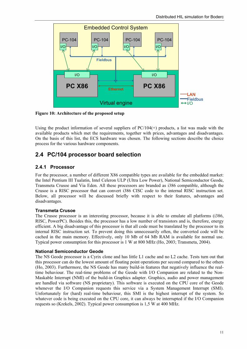
2.3.2 Virtual Engine To run the simulation models for Hardware-In-the-Loop simulation, the virtual engine needs one (or more) powerful processing units that are able to simulate the dynamics of the paper path in real-time (calculations and I/O for generation of new output signals should be finished before the next sample moment). Code generation will be used to generate the required software for this HIL simulator. The preferred hardware for the virtual engine is COTS PC X86 hardware (Visser and Broenink, 2003). This results, together with the requirements for the ECS in the global architecture depicted in Figure 10. For efficient use of the HIL simulator and the ECS, a comfortable experimental environment is required. A first step for this is using 20-sim in combination with automated code generation to one of the ECS PC’s and a single HIL simulator. Relevant signals can be visualized for analysis in 20-sim using recorded data or, if possible, on-line using data logging via a network connection during a HIL simulation experiment.
Distributed HIL simulation for Boderc
11
PC-104I/O
Fieldbus
Virtual engine
PC X86
I/O
PC X86
I/O
Ethernet
Embedded Control System
I/OFieldbusLAN
PC-104I/O
PC-104I/O
PC-104I/O
PC-104I/O
PC-104I/O
Fieldbus
Virtual engine
PC X86
I/O
PC X86
I/OI/O
PC X86
I/O
PC X86
I/OI/O
Ethernet
Embedded Control System
I/OFieldbusLAN
PC-104I/O
PC-104I/O
PC-104I/O
PC-104I/O
PC-104I/O
PC-104I/O
Figure 10: Architecture of the proposed setup
Using the product information of several suppliers of PC/104(+) products, a list was made with the available products which met the requirements, together with prices, advantages and disadvantages. On the basis of this list, the ECS hardware was chosen. The following sections describe the choice process for the various hardware components.
2.4 PC/104 processor board selection
2.4.1 Processor For the processor, a number of different X86 compatible types are available for the embedded market: the Intel Pentium III Tualatin, Intel Celeron ULP (Ultra Low Power), National Semiconductor Geode, Transmeta Crusoe and Via Eden. All these processors are branded as i386 compatible, although the Crusoe is a RISC processor that can convert i386 CISC code to the internal RISC instruction set. Below, all processor will be discussed briefly with respect to their features, advantages and disadvantages.
Transmeta Crusoe The Crusoe processor is an interesting processor, because it is able to emulate all platforms (i386, RISC, PowerPC). Besides this, the processor has a low number of transistors and is, therefore, energy efficient. A big disadvantage of this processor is that all code must be translated by the processor to its internal RISC instruction set. To prevent doing this unnecessarily often, the converted code will be cached in the main memory. Effectively, only 10 Mb of 64 Mb RAM is available for normal use. Typical power consumption for this processor is 1 W at 800 MHz (Ho, 2003; Transmeta, 2004).
National Semiconductor Geode The NS Geode processor is a Cyrix clone and has little L1 cache and no L2 cache. Tests turn out that this processor can do the lowest amount of floating point operations per second compared to the others (Ho, 2003). Furthermore, the NS Geode has many build-in features that negatively influence the real-time behaviour. The real-time problems of the Geode with I/O Companion are related to the Non-Maskable Interrupt (NMI) of the build-in Graphics adapter. Graphics, audio and power management are handled via software (NS proprietary). This software is executed on the CPU core of the Geode whenever the I/O Companion requests this service via a System Management Interrupt (SMI). Unfortunately for (hard) real-time behaviour, this SMI is the highest interrupt of the system. So whatever code is being executed on the CPU core, it can always be interrupted if the I/O Companion requests so (Krekels, 2002). Typical power consumption is 1,5 W at 400 MHz.

Distributed HIL simulation for Boderc
12
Via Eden ESP Also the Via Eden is a Cyrix clone. It is equipped with 192 kb combined L1/L2 cache. The FPU (Floating Point Unit, used for floating point calculations) is less powerful than a comparable Intel Celeron ULP. This is a point of attention if a lot of floating point operations will be performed. The processor is specially targeted for the low power embedded market. Compared with Intel’s Celeron processor, this processor has a smaller number of transistors because it does not implement the complete i386 instruction set in hardware. The CPU is optimized for frequently used instructions (like MOV, ADD etc.). Those instructions are very fast. Instructions that are rarely used, will be emulated by the CPU (Via, 2003). The Eden processor is available as 400, 666, 800 and 1 GHz processor and is cheaper than comparable Celeron processors. A fan is only required for the 1 GHz version. The Via Eden processor will stay in production for at least the next 3 years. Typical power consumption is 3.2 W at 666 MHz.
Intel Celeron/Pentium A Intel Pentium III embedded processor is the most powerful of all discussed processors. It is also the most expensive processor with the highest power consumption and heat dissipation. The normal Pentium and Celeron processors are almost all equipped with a fan above 600 MHz. Intel has also an ultra low power (ULP) version of the Celeron which does not need a fan but it turned out that Intel has already stopped the production of this processor.
Comparison and choice Comparing all processors, the Crusoe and the Geode processor are eliminated directly. The choice stays between the Eden and the Pentium/Celeron processor. Comparing the prices of these processors at the same clock speed, the Pentium III (embedded) is the most expensive one, followed by the Celeron. The prices of a 400 MHz Celeron are comparable to a 600 MHz Via Eden, but the production of the Intel CPU’s is already stopped. Conclusion: the best choice is the Via Eden processor.
2.4.2 Network & Flash card One of the requirements for the demo setup is the ability to configure the demo setup via a network link. One of the possibilities for remote configuration is to boot the PC/104’s from the network. In this way, the configuration for the entire setup can be changed at one central place (remote boot server). Besides for remote configuration, the network can also be used for remote control (start/stop programs) of the demo setup. The PC’s should therefore be equipped with at least a 10 Mbit network interface and network boot capabilities. It turned out that almost none of the PC/104 CPU boards has the possibility to boot from the network. For this, an alternative must be found in booting from floppy, hard disk or flash card (Disk on Chip, Disk on Module or Compact Flash)2. An advantage of a flash card is the possibility to keep a local installation of the operating system. This is useful when the setup needs to be transported for a demonstation.
2.5 CAN board selection No processor boards with an onboard CAN controller could be found with a CPU faster that 133 MHz. So, a separate PC/104(+) extension board is required. Different vendors offer various CAN boards with one or two separate CAN controllers. A choice exists for different CAN controllers like Philips SJA 1000 and Intel 82527. The most sold and used CAN controller is the Philips SJA1000. The Intel 82527 has a receive buffer for 15 messages of 8 bytes and the SJA1000 for 8 messages. The SJA1000 has a number of advantages (single-shot transmission, hot-plugging support) over the 82527 that could be useful for the HILs setup. Single shot transmission is for example required for hard real-time communication (retransmission after an error of time specific information is not desirable). Therefore, the preference is given to the SJA1000 CAN controller. Besides the controller, it is also important that the vendor supplies DOS and/or Linux drivers or sample source code. Not all vendors provide Linux drivers or source code that can be used to write own drivers. Boards with only Windows drivers are not useful for this setup.
2 In the mean time, the Via Eden boards from Seco are equipped with a new BIOS with network boot capabilities.

Distributed HIL simulation for Boderc
13
2.6 Power supply The setup requires also at least one power supply for all PC/104 pc’s. It is possible to use special PC/104 power supplies, which fit into the PC/104 stack, but they have one disadvantage: they are expensive (around 10 times the price of a standard PC power supply). The demo setup will consist of four PC/104 pc’s mounted together with some additional I/O hardware. It is possible to connect all PC/104’s to one standard PC power supply, but this has the disadvantage that it is not possible to switch on/off all PC/104’s individually. There is a small PC power supply (150 W microATX) on the market that has dimensions similar to a PC/104 stack for a price comparable to a standard PC power supply. This power supply makes it possible to have one power supply per PC/104 and connect extra I/O hardware directly to the power supply, keeping the demo setup compact and portable.
2.7 Display For the PC/104 PC’s it is not required to connect a VGA display to the PC when running some controller software. However, for demonstation and testing purposes, it would be convenient to have a small display per PC/104 to show status information. For this purpose, a small text-based LCD screen connected to the parallel port will be used.
2.8 Final hardware choice The final hardware choice is made in favour of the Seco M570 PC104+ CPU board with an 600 MHz Via Eden CPU, supplied with 256 MB RAM and a 32 MB Flashdisk. For CAN fieldbus support, the choice was made for the Peak System PCAN PC104 board with the SJA1000 controller. For more detailed information about these boards, see Table 1 and appendix I.
Description 4x Seco M570 BAB Via Eden 600 MHz 4x Connection Cable kit M570 4x SoDimm 256 MB 4x 32 MB Flash Disk on Module (boot) 4x PCAN PC104 opto 1xCAN SJA1000 1Mb/s 4x microATX power supply Various cables (CAN, power, UTP) Networkswitch 8 poorts UTP 4x 16x4 dot matrix LCD
Table 1: ECS setup
2.9 Operating System The past sections described the hardware requirements for the ECS setup, but nothing was said about the accompanying operating system and software requirements. This section describes these software requirements and the motivation of the choice process.
2.9.1 Requirements To boot the ECS PC’s an operating system is required. The operating system should be able to run CTC(++) programs and 20-sim models (via code-generation). An operating system with hard real-time capabilities is required for the ECS setup. At the Control Laboratory, both DOS and (RT)Linux are in use for this purpose. DOS is a simple 16-bit operating system without multitasking capabilities and can therefore be considered as real-time capable. Linux itself is not capable of guaranteeing the predictable time limits needed for real-time tasks. The Linux kernel is designed to optimise average performance. This means that all processes will get a fair share of CPU time. For real-time programs precise timing and predictable timing is more important than average performance. Therefore, Linux needs some real-time extensions like RTlinux or RTAI, which combines a hard-real-time kernel (e.g. Adeos or RTHAL) with the normal Linux kernel. See for more information (Stephan, 2002).
Distributed HIL simulation for Boderc
14
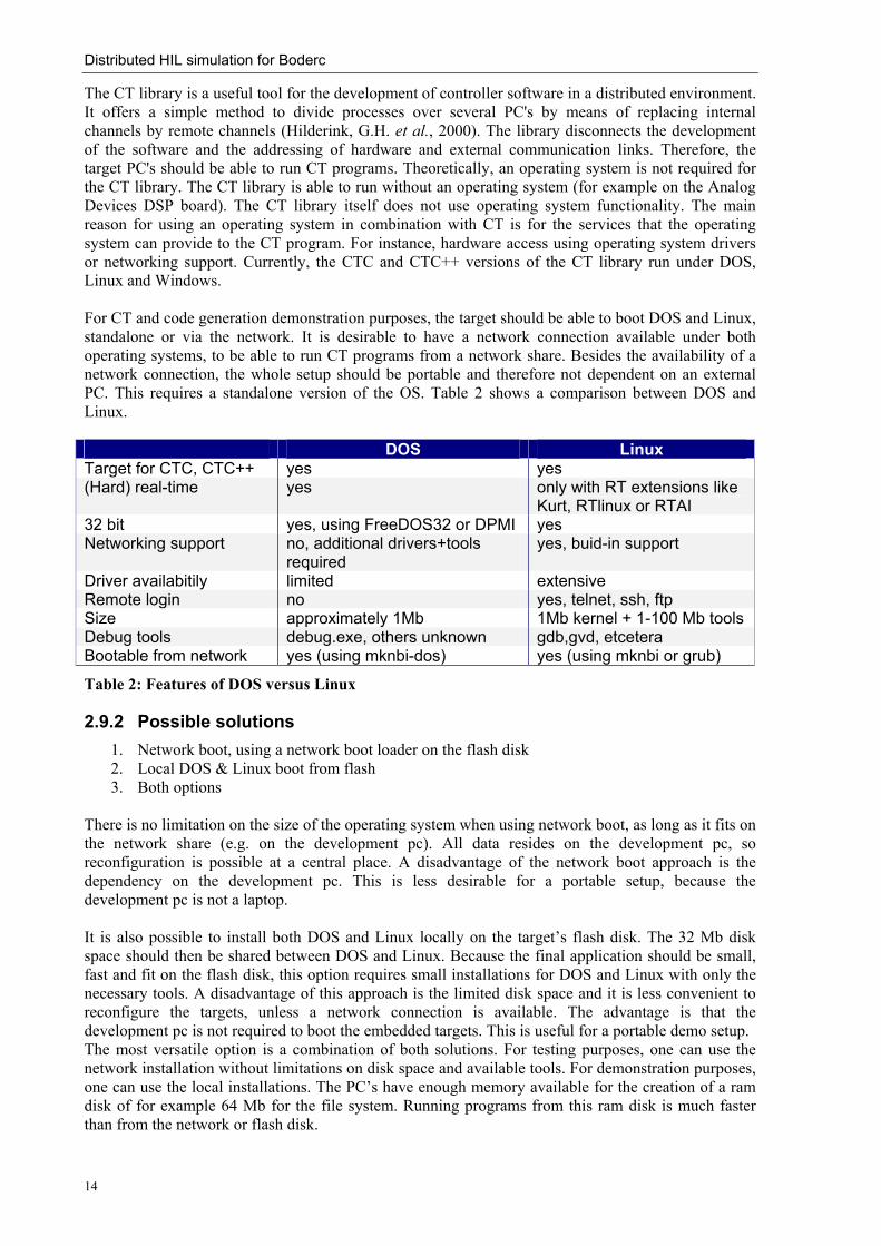
The CT library is a useful tool for the development of controller software in a distributed environment. It offers a simple method to divide processes over several PC's by means of replacing internal channels by remote channels (Hilderink, G.H. et al., 2000). The library disconnects the development of the software and the addressing of hardware and external communication links. Therefore, the target PC's should be able to run CT programs. Theoretically, an operating system is not required for the CT library. The CT library is able to run without an operating system (for example on the Analog Devices DSP board). The CT library itself does not use operating system functionality. The main reason for using an operating system in combination with CT is for the services that the operating system can provide to the CT program. For instance, hardware access using operating system drivers or networking support. Currently, the CTC and CTC++ versions of the CT library run under DOS, Linux and Windows. For CT and code generation demonstration purposes, the target should be able to boot DOS and Linux, standalone or via the network. It is desirable to have a network connection available under both operating systems, to be able to run CT programs from a network share. Besides the availability of a network connection, the whole setup should be portable and therefore not dependent on an external PC. This requires a standalone version of the OS. Table 2 shows a comparison between DOS and Linux.
DOS Linux Target for CTC, CTC++ yes yes (Hard) real-time yes only with RT extensions like
Kurt, RTlinux or RTAI 32 bit yes, using FreeDOS32 or DPMI yes Networking support no, additional drivers+tools
required yes, buid-in support
Driver availabitily limited extensive Remote login no yes, telnet, ssh, ftp Size approximately 1Mb 1Mb kernel + 1-100 Mb tools Debug tools debug.exe, others unknown gdb,gvd, etcetera Bootable from network yes (using mknbi-dos) yes (using mknbi or grub)
Table 2: Features of DOS versus Linux
2.9.2 Possible solutions 1. Network boot, using a network boot loader on the flash disk 2. Local DOS & Linux boot from flash 3. Both options
There is no limitation on the size of the operating system when using network boot, as long as it fits on the network share (e.g. on the development pc). All data resides on the development pc, so reconfiguration is possible at a central place. A disadvantage of the network boot approach is the dependency on the development pc. This is less desirable for a portable setup, because the development pc is not a laptop. It is also possible to install both DOS and Linux locally on the target’s flash disk. The 32 Mb disk space should then be shared between DOS and Linux. Because the final application should be small, fast and fit on the flash disk, this option requires small installations for DOS and Linux with only the necessary tools. A disadvantage of this approach is the limited disk space and it is less convenient to reconfigure the targets, unless a network connection is available. The advantage is that the development pc is not required to boot the embedded targets. This is useful for a portable demo setup. The most versatile option is a combination of both solutions. For testing purposes, one can use the network installation without limitations on disk space and available tools. For demonstration purposes, one can use the local installations. The PC’s have enough memory available for the creation of a ram disk of for example 64 Mb for the file system. Running programs from this ram disk is much faster than from the network or flash disk.
Distributed HIL simulation for Boderc
15
2.9.3 PC/104 OS installation – final choice Using Table 2 and the list of requirements, the final choice for the OS is made in favour of Linux together with RTAI. This is mainly due to the limited driver availability of DOS and the lack of network support for remote configuration. To install a RTAI Linux system, a normal Linux installation is required with a slightly modified kernel and some additional kernel modules that modify the behaviour of the Linux kernel in such a way that a better real-time performance can be guaranteed when needed. The best way to install Linux on an embedded PC/104 system is from scratch, by adding only the tools that are really required. The installation of a custom Linux installation with real-time extensions is not straightforward and took a couple of weeks to complete. To facilitate the installation in the future, Appendix IV describes the installation process for the creation of a RTAI Linux installation from scratch. The created Linux installation uses a non-standard C library, called uClibc (Andersen, 2004), which is designed to reduce the size of the standard Glibc library on embedded targets. The embedded Linux installation has no onboard compilers because of their size. To compile new software for this Linux installation, a Linux development PC is required with a uClibc cross compiler (see (Andersen, 2004) for the creation of the required cross compiler tool chain). This custom Linux installation takes approximately 10 Mb diskspace, boots into a ram disk and can be installed on the flash disk, leaving enough space available for a small DOS installation with networking support. A special uClibc cross compiler for Windows (Cygwin) is created to facilitate the automation of 20-sim codegeneration to the embedded Linux installation without the intervention of a Linux development machine for the compilation process. The resulting OS installation for the PC/104 PC’s consists of both a local DOS and a local Linux installation and the possibility to boot the PC/104 PC’s from the network with both DOS and Linux.


Distributed HIL simulation for Boderc
17
3 HIL simulation setup I/O interface
3.1 Introduction This chapter has been entirely dedicated to the I/O interface of the ECS and the HIL simulator. A significant part of the distributed HIL simulation setup is the boundary between the control system and the emulated hardware. This chapter will explain the possible forms of I/O and the possibilities for the HIL simulator and the ECS concerning I/O. Then a short explanation, concerning the possibilities with respect to the I/O hardware choice, follows. The last sections of this chapter describe the chosen I/O board, the written Linux drivers for this I/O board and the use of the board for both the ECS and the HIL simulator.
3.2 Input/Output The coupling of the HIL simulator and the ECS can be subdivided into a sensor interface and an actuator interface (see Figure 11). The sensor interface generates the necessary sensor signals and the actuator interface will consist mainly of output drivers for motor steering. Before discussing the alternatives for I/O hardware on the HIL simulation setup, first a brief introduction into the basics of input and output are given from the perspective of a (real-time) computer system.
Signal conditioning Controller
Sensor simulation
Output driver
Embedded Control System
Model of the plant
Hardware-In-the-Loop simulator
A/D, PWM, etc.D/A, encoder, etc.
Actuator simulation
Electrical interface Electrical interface
Signal conditioning
Signal conditioning ControllerController
Sensor simulation
Sensor simulation
Output driverOutput driver
Embedded Control System
Model of the plantModel of the plant
Hardware-In-the-Loop simulator
A/D, PWM, etc.D/A, encoder, etc.
Actuator simulationActuator
simulation
Electrical interface Electrical interface
Figure 11: I/O interface of a typical HIL simulation setup (repetition of Figure 3)
3.2.1 Time Every I/O signal has two dimensions, its value and the time. This time can have different roles in a real-time system (Kopetz, 1997):
• Time as data: time of a value change is important of later analysis of the consequences of the event, e.g. how long did an event endure.
• Time as control: a value change may require immediate action of the computer system, e.g. for an airbag sensor.
In the context of computer hardware, the values are the contents of a register and the time is the trigger moment at which the register contents are transferred to another subsystem. The role of the time for a particular I/O signal, gives different requirements for the hardware and software. Delay is critical in a time-as-control situation. These kind of signals require minimal delays and must be treated in hard real-time. On the other hand, in the time-as-data situation, a global time base is more important than a minimal delay. Some delay is no problem, as long as the delay is known. E.g. a control action that should occur precisely at the intended moment: the next sample time.

Distributed HIL simulation for Boderc
18
3.2.2 Sampling, polling, interrupts Different ways exist for observing the state of an input value. Observing the value on equidistant times is called equtemporal sampling. The time interval between two samples is constant. Polling and sampling are almost the same. With sampling, the sensor keeps the last known value until the computer reads its value and with polling, the computer plays the role of memory. With polling, the computer reads only the most recent value and events that occur between two sampling point are not ‘seen’. Polling is enough if only the most recent value is of interest. If every event (state change) is important, one should use sampling. Using interrupts, the change in the status of an input value can interrupt the running software and start an interrupt service routine to service the event.
3.2.3 Sensors & actuators The types of the sensors and actuators are important for the choice of the I/O. It is not just analog or digital I/O that is required (Kopetz, 1997). Below various types of possible sensor/actuator I/O signals are given.
analog I/O
sensors & actuators
digital I/O intelligent instrumentationsensors with build-in intelligence. Real sensor/actuator interface is hidden behind a build-in microcontroller. Some sensors/actuators can be connected directly to a standard I/O interface or field bus.
• current
• voltage
• frequency
• state: on/off
• value: binary, parallel
• time encoded: PWM, position encoder, frequency, serial links
Figure 12: Various I/O signals
The exact types of the sensors and actuators on the copier determine the requirements of the I/O boards.
3.2.4 Types of I/O access Input and output of data to and from a computer system is accomplished through one of the following three methods:
• Programmed I/O • Memory-mapped I/O • Direct memory access (DMA)
Interrupt driven I/O access can be seen as the fourth method for I/O access. However, it is an implementation of one of the above methods in which an interrupt signals the completion of an I/O transfer or a request for an I/O transfer. With programmed I/O, the CPU is involved in the transfer of I/O data. These CPU efforts cost time (approximately 1 µs per inbyte/outbyte call, independent on the speed of the X86 PC) which must be taken into account for the real-time performance. Memory mapped I/O provides access to I/O data via designated memory locations that work as virtual input/output ports. Memory-mapped I/O is faster than programmed I/O, if the response time of the corresponding I/O device is similar to the response time of regular memory. Direct memory acces gives I/O devices access to the memory without CPU intervention, resulting in a faster data transfer from and to the memory. The disadvantage of DMA is that the CPU cannot

Distributed HIL simulation for Boderc
19
perform a data transfer during DMA. The CPU has to wait (or proceed with calculations that do not require external data) until the DMA controller allows the CPU data transfer. This influences the real-time behaviour when a lot of data is transferred using DMA. HIL simulation does not require large data transfers, so DMA is not required, however memory mapped I/O would be useful for the HIL simulator.
3.2.5 A/D-D/A hardware A/D-D/A hardware provides analog-to-digital (AD) and digital-to-analog conversion, or continuous to discrete and discrete to continuous signal conversion. The key factor in the service of A/D and D/A hardware is the sampling frequency. An A/D convertor requires at least 2000 samples per second for a 1000 Hz signal (two times the Nyquist frequency). This requires that software tasks serving this A/D hardware also must run at at least this sampling rate without loss of information. The required sampling frequency and software speed depends on the frequency of the analog signal. Besides the sampling frequency, the number of bits of an AD or DA convertor determines the measurement accuracy and the quantization error. Because A/D conversion takes time, it reduces the available time interval between the occurrence of a specific value and the use of this value for an output action.
3.3 HIL simulator and its I/O
3.3.1 HIL simulator input/output For a typical3 HIL simulation setup, all I/O on the HIL simulator is exactly the same as on the real hardware. When the controller has an analog output, the HIL simulator needs an AD converter. When the controller controls a motor, the controller output is for example a PWM signal and the required input is a position encoder signal. The HIL simulator must have a counterpart for each of the controller inputs and outputs (see also Figure 11). The testcase is the HIL simulator (the virtual engine) for the paper path of an Océ Varioprint™ copier. Figure 13 depicts a 20-sim model of the virtual engine.
Figure 13: 20-sim model for the virtual engine (Berg, 2003)
The paper path controller has the following inputs and outputs:
Inputs: • Quadrature encoder signals: four motors are equipped with position encoders. The maximum
frequency is around 200 kHz. • Digital signals: sensors for paper detection and stop position.
3 Often used in (automotive) industry
Sheets
Sensor1
Flip1
Flip2
Feeder
Finisher
Controller
Sensor2Sensor3
Sensor4
Sensor5
Sensor6
Sensor7
Sensor8 FUSE
Pinch0 Pinch1 Pinch2
Pinch3
Pinch4
Pinch5
Pinch6 Pinch7
Pinch8
Pinch9
Pinch10
Pinch11 Pinch12
Distributed HIL simulation for Boderc
20
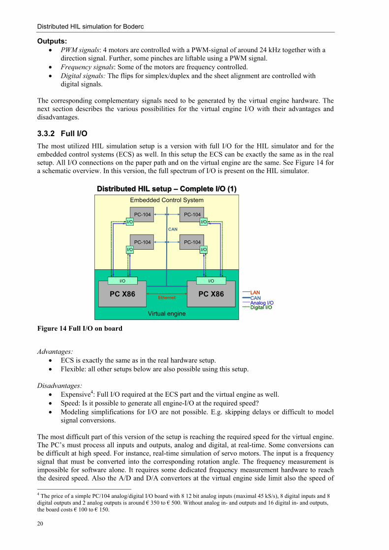
Outputs: • PWM signals: 4 motors are controlled with a PWM-signal of around 24 kHz together with a
direction signal. Further, some pinches are liftable using a PWM signal. • Frequency signals: Some of the motors are frequency controlled. • Digital signals: The flips for simplex/duplex and the sheet alignment are controlled with
digital signals. The corresponding complementary signals need to be generated by the virtual engine hardware. The next section describes the various possibilities for the virtual engine I/O with their advantages and disadvantages.
3.3.2 Full I/O The most utilized HIL simulation setup is a version with full I/O for the HIL simulator and for the embedded control systems (ECS) as well. In this setup the ECS can be exactly the same as in the real setup. All I/O connections on the paper path and on the virtual engine are the same. See Figure 14 for a schematic overview. In this version, the full spectrum of I/O is present on the HIL simulator.
Distributed HIL setup Distributed HIL setup –– Complete I/O (1)Complete I/O (1)
PC-104I/O
PC-104I/O
PC X86
I/O
PC-104I/O
PC-104I/O
PC X86
I/O
CAN
Virtual engine
Ethernet
Embedded Control System
Digital I/OAnalog I/OCANLAN
Distributed HIL setup Distributed HIL setup –– Complete I/O (1)Complete I/O (1)
PC-104I/O
PC-104I/O
PC-104I/O
PC-104I/O
PC X86
I/O
PC X86
I/OI/O
PC-104I/O
PC-104I/O
PC-104I/O
PC-104I/O
PC-104I/O
PC-104I/O
PC X86
I/O
PC X86
I/OI/O
CAN
Virtual engine
Ethernet
Embedded Control System
Digital I/OAnalog I/OCANLAN
Figure 14 Full I/O on board
Advantages:
• ECS is exactly the same as in the real hardware setup. • Flexible: all other setups below are also possible using this setup.
Disadvantages:
• Expensive4: Full I/O required at the ECS part and the virtual engine as well. • Speed: Is it possible to generate all engine-I/O at the required speed? • Modeling simplifications for I/O are not possible. E.g. skipping delays or difficult to model
signal conversions. The most difficult part of this version of the setup is reaching the required speed for the virtual engine. The PC’s must process all inputs and outputs, analog and digital, at real-time. Some conversions can be difficult at high speed. For instance, real-time simulation of servo motors. The input is a frequency signal that must be converted into the corresponding rotation angle. The frequency measurement is impossible for software alone. It requires some dedicated frequency measurement hardware to reach the desired speed. Also the A/D and D/A convertors at the virtual engine side limit also the speed of 4 The price of a simple PC/104 analog/digital I/O board with 8 12 bit analog inputs (maximal 45 kS/s), 8 digital inputs and 8 digital outputs and 2 analog outputs is around € 350 to € 500. Without analog in- and outputs and 16 digital in- and outputs, the board costs € 100 to € 150.

Distributed HIL simulation for Boderc
21
the virtual engine. The response time (or delay between input and output) determines how much time is available for the virtual engine to calculate the corresponding analog output value for a specific analog input value. This is a generic problem of HIL simulation. The HIL simulator is always slower in calculation of its state (e.g. paper position) than a physical process, which always has its state available (paper position is always visible). This is comparable to sampling versus analogue signals. A possible solution for this is the use of a dedicated processor for the high speed signal generation part of the virtual engine, like a DSP or microcontroller (Berg, 2003). This situation is depicted in Figure 15, where a microcontroller takes care of some part of the virtual engine I/O. The microcontroller prepares the I/O signals for the PC in such a way that the converted I/O can easily be fed into the PC without spending too much time on the conversion of signals into a calculatable format. This leaves more time available for the virtual engine PC to calculate the required output signals.
Analog I/O
Distributed HIL setup Distributed HIL setup –– Complete I/O (2) Complete I/O (2)
PC-104I/O
PC-104I/O
PC X86
I/O using µC
PC-104I/O
PC-104I/O
PC X86
I/O using µC
CAN
Virtual engine
Ethernet
Embedded Control System
Digital I/O
CANLAN
µC
PC X86
Input Output
µC µC
I/O pre- andpostprocessing
using a microcontroller
Analog I/O
Distributed HIL setup Distributed HIL setup –– Complete I/O (2) Complete I/O (2)
PC-104I/O
PC-104I/O
PC-104I/O
PC X86
I/O using µC
PC-104I/O
PC-104I/O
PC-104I/O
PC-104I/O
PC-104I/O
PC-104I/O
PC X86
I/O using µC
CAN
Virtual engine
Ethernet
Embedded Control System
Digital I/O
CANLAN
µC
PC X86
Input Output
µC µC
I/O pre- andpostprocessing
using a microcontroller
Figure 15: Virtual engine with microcontrollers
Figure 16 depicts a simple example of a motor controller with temperature protection. The microcontroller converts for example the PWM signal into a position and the angle from the HIL simulator into encoder pulses. Besides this, the motor temperature will be converted by a D/A converter into the sensor voltage. The interface with the HIL simulator computer is now completely digital.
Figure 16: Example of a motor controller with temperature protection

Distributed HIL simulation for Boderc
22
3.3.3 Partial I/O It is questionable whether it is required to have a full spectrum of I/O connections available on the virtual engine, like A/D, digital (serial and parallel). When the embedded controller has a DA converter and the corresponding HIL simulator input is an AD converter, it is possible to skip the DA-AD part because this is not required for testing the control software. This situation is depicted in Figure 17.
Digital I/OAnalog I/O
Distributed HIL Distributed HIL setup setup –– No analog I/ONo analog I/O
PC-104I/O
PC-104I/O
PC X86
I/O
PC-104I/O
PC-104I/O
PC X86
I/O
I/O
CAN
Virtual engine
Ethernet
Embedded Control System
CANLAN
Digital I/OAnalog I/O
Distributed HIL Distributed HIL setup setup –– No analog I/ONo analog I/O
PC-104I/O
PC-104I/O
PC X86
I/O
PC-104I/O
PC-104I/O
PC X86
I/O
I/O
CAN
Virtual engine
Ethernet
Embedded Control System
CANLAN
Distributed HIL Distributed HIL setup setup –– No analog I/ONo analog I/O
PC-104I/O
PC-104I/O
PC-104I/O
PC-104I/O
PC X86
I/O
PC X86
I/OI/O
PC-104I/O
PC-104I/O
PC-104I/O
PC-104I/O
PC-104I/O
PC-104I/O
PC X86
I/O
PC X86
I/OI/O
I/O
CAN
Virtual engine
Ethernet
Embedded Control System
CANLAN
Figure 17: No analog I/O
Advantages:
• Cheaper: no expensive analog I/O hardware required. • No changes in the controller software required (except for the I/O hardware drivers).
Disadvantages:
• I/O delay: the effects of the AD/DA conversion time and noise on the controller stay unknown. Further, the speed limitations for AD conversion are omitted which allows for a speed up that is not possible with the real analog hardware.
• Quantization effects stay unknown or need to be modelled at the virtual engine side. An advantage of the modelling is that this allows for changing the number of bits.
• Effects of noise on analog signals are not present. • The Embedded Control System hardware cannot be used directly in the real setup, because
some I/O hardware is different. The ECS is only suitable for functional tests of the software and hardware platform.
3.3.4 I/O Simulation It is also possible to go one step further in crossing off I/O by simulating a portion of the I/O by shifting the border between the ECS and the virtual system towards the ECS. Not mission critical I/O like monitoring signals can also be send to a embedded PC using the on board LAN connection. It can be seen as an I/O tunnel via Ethernet. To make this work, a small part of the HIL simulator must run on the embedded PC for translation of the Ethernet messages into I/O; a pseudo-I/O driver. This situation is depicted in Figure 18. The virtual engine is still responsible for all hardware simulation.

Distributed HIL simulation for Boderc
23
Distributed HIL Distributed HIL setup setup –– Partial I/O simulationPartial I/O simulation
PC-104I/O
PC-104I/O
PC X86
I/O
PC-104I/O
PC-104I/O
PC X86
I/O
CAN
Virtual engine
Ethernet
Embedded Control System
Digital I/OAnalog I/OCANLANI/O simulation
Distributed HIL Distributed HIL setup setup –– Partial I/O simulationPartial I/O simulation
PC-104I/O
PC-104I/O
PC-104I/O
PC-104I/O
PC X86
I/O
PC X86
I/OI/O
PC-104I/O
PC-104I/O
PC-104I/O
PC-104I/O
PC-104I/O
PC-104I/O
PC X86
I/O
PC X86
I/OI/O
CAN
Virtual engine
Ethernet
Embedded Control System
Digital I/OAnalog I/OCANLANI/O simulation
Figure 18: Partial I/O simulation
Advantages: • Cheaper: Less I/O is needed for the testing. • Simple addition of virtual I/O possible making it possible to test the effects of extra sensors
without the requirement for additional hardware. Disadvantages:
• Part of the HIL simulation software runs on the ECS under test. Higher CPU load. This requires changes in both the ECS and the HIL simulator.
• Not very suitable for hard-real time communication because of the unpredictable latencies and extra delay for the transportation via LAN. Switching to real-time Ethernet (RT-NET) may help in reducing the unpredictable latencies.
It is even possible to skip all I/O and transport all I/O information via (a dedicated) LAN connection to the ECS under test. This situation is depicted in Figure 19 which looks like model-in-the-loop. This setup requires a good knowledge about the differences between the Ethernet transfer of the I/O signals and the real I/O situation. It requires the use of RT-net, otherwise the variable transmission latencies will give unpredictable results. The best way to use this setup will be together with real-time simulation of the I/O effects (delays, quantization) using toolboxes like TrueTime and Jitterbug (Cervin et al., 2002). It can also be used for non-real-time simulation methods like Processor-In-the-Loop (testing of the generated controller code on the target hardware architecture) earlier in the design trajectory.
Distributed HIL Distributed HIL setup setup –– I/O simulationI/O simulation
PC-104
PC-104
PC X86
PC-104
PC-104
PC X86
CAN
Virtual engine
Ethernet
Embedded Control System
Digital I/OAnalog I/OCANLANI/O simulation
Distributed HIL Distributed HIL setup setup –– I/O simulationI/O simulation
PC-104
PC-104
PC X86
PC-104
PC-104
PC X86
CAN
Virtual engine
Ethernet
Embedded Control System
Digital I/OAnalog I/OCANLANI/O simulation
Figure 19: Only virtual I/O

Distributed HIL simulation for Boderc
24
3.3.5 Conclusions and remarks Table 1 summarizes the most important features of the discussed I/O options. For the paperpath controller it is not required to have A/D and D/A convertors analog signals. All signals described in section 3.3.1 are digital signals. The most feasible setup is therefore the digital only setup from Figure 17, eventually extended with dedicated microcontroller/DSP hardware for digital signal conversion (PWM generation, encoder count, frequency generation).
Option Advantages Disadvantages Full I/O HILs/ECS equal to real setup expensive Digital I/O suitable for virtual engine no analog I/O I/O simulation unlimited I/O possiblities Performance dependent on
communication link Simulation on the ECS Requires lots of changes
extension with µc/DSP no PC processing power for signal conversion
separate hardware required
Table 3: Comparison I/O options
3.4 I/O Hardware choice In the previous section, the requirements put to the I/O hardware of the HIL simulator PC. To prevent searching twice for suitable I/O hardware for both the controller and the HIL simulator, the choice was made to search for one board, both useable for the HIL simulator and the ECS. This saves time for writing device drivers and prevents compatibility issues (e.g. different signal levels). A second advantage is that the first HIL simulation experiments can be performed on one of the ECS PC’s. The FPGA based Anything I/O board from Mesa Electronics (Mesa, 2000) satisfies all requirements from section 3.3.1. This Anything I/O board is fully customizable to I/O requirements for both the ECS and the HIL simulator for a competing price compared to other COTS digital I/O boards. Feature summary:
• Xilinx Spartan FPGA • Completely configurable using VHDL or Verilog or similar hardware languages • Competing price • PC104+ and PCI version available • 72 general purpose digital I/O pins • IRQ generation capable • Programmed I/O and memory mapped I/O
This board guarantees high flexibility in forming the required pulses for both the sensor and actuator side of the virtual engine as long as all signals are digital. The FPGA can handle all required signal conversions for the virtual engine PC like in the DSP/microcontroller situation (see Figure 15), It is possible to connect the FPGA I/O boards on the ECS PC’s with each other to provide synchronized sampling (all PC’s are triggered via one central clock). The use of this FPGA I/O board is not limited to HIL simulation. The flexibility of the FPGA configurations enables a much broader range of applications. The main limitation of the board is that it has no analog I/O. The board can be extended in the future with AD and DA convertors for a connection to the analog domain. The Anything I/O hardware can do the sampling, while the software reads/writes only from/to the I/O registers. The next section describes the Anything I/O board in more detail.
3.5 Anything I/O board hardware The Anything I/O board is built around a Xilinx Spartan FPGA and a PCI bridge. Figure 20 depicts the layout of the board.

Distributed HIL simulation for Boderc
25
Figure 20: Anything I/O board layout
3.5.1 I/O interface The Anything I/O board provides 72 general purpose I/O pins divided over three connectors with removeable pull up resistors. All pins can drive a current of maximal 24 mA. The voltage level of the pins is maximal 5 V, depending on the chosen I/O standard. The FPGA supports multiple I/O standards like 5V TTL and 3.3V CMOS. Warning: The outputs of the Anything I/O board have no external buffering. An accidental short
circuit, wrong I/O standard or interchange of input and output may end into FPGA damage. Be sure to double-check all connections
3.5.2 PCI Interface The PCI interface is a PLX 9030 from PLX Technology. It is a 32Bit, 33MHz Slave interface chip with a local bus that can be run up to 60MHz. This local bus provides a data path between the PLX9030 and the Xilinx Spartan FPGA. The PLX local bus interface uses a 32 bit multiplexed address/data bus. For more information see appendix VII and the datasheet.
3.5.3 JTAG Interface The JTAG interface allows for device configuration and boundary scan testing of the Xilinx FPGA. The JTAG interface is useful for debugging new FPGA configurations with suitable JTAG PC hardware. A JTAG PC interface is available at the Control Laboratory.
3.5.4 Xilinx FPGA The used Xilinx FPGA has 200.000 system gates and 56 k blockram and can run up to 200 MHz. A 50 MHz crystal oscillator is provided as the FPGA system clock. Also, the 33 MHz PCI clock is available to the FPGA. Higher or lower frequencies can be generated by the 4 DLLs (Delay Locked Loop) built into FPGA. The FPGA configuration can be downloaded on demand, via the PCI bus and is lost after a reboot. Sample configurations are available that provide PWM and encoder I/O, general purpose I/O and a FPGA based microcontroller for servo motor control. The Xilinx ISE Webpack and ModelSim XE Limited software packages (Xilinx, 2004) can be used for the development of new FPGA configurations. These tools can be downloaded for free from the Xilinx website. Appendix VI gives a small getting started manual for the ISE Webpack software.
PLX 9030 PCI interface
PCI bus (33 MHz)
Xilinx Spartan XC2s200 FPGA
JTAG
I/O 1 (24 pins)
I/O 2 (24 pins)
I/O 3 (24 pins)
Configuration EEPROM
8 programmable status LEDs (green)
2 status LEDs (red, yellow)
Program led Local bus 60 MHz
50 MHz osc.

Distributed HIL simulation for Boderc
26
3.6 Anything I/O driver for Linux Mesa Electronics does not deliver any drivers or tools to program and use the Anything I/O boards under Linux. Only sample sources for programming under DOS and Windows are available. To program the Anything I/O board and to access its I/O ports, a Linux driver, called Anyio, was written. This section describes the basics of the driver.
3.6.1 Supported hardware The Anyio Linux driver is intended for both versions of the Mesa Anything I/O board, the PCI version (5I20) as well as the PC104+ version (4I65). The driver was written for the Linux 2.4 kernel, although the source contains some code to make the module compatible with the older 2.2 version of the Linux kernel.
3.6.2 Driver Structure The Anyio driver consists of two parts: a kernel module (required) for hardware access and a small library for userspace communication with the kernel module. Figure 21 explains the structure of the Anything I/O driver. This structure is similar to the common Linux way for hardware access using the device filesystem as described in (Rubini and Corbert, 2001).
User space
libanyiodevice filesystem/dev/anyio/proc/anyio
X
Linux shelle.g. programming:# cp io24.bit /dev/anyio0
CTC++ programanyio linkdriver
Kernel space
anyio module
Linux 2.4 kernel
Hardware
Mesa Anything I/O board
FPGAPLX 9030
other software
PLXI/O
MEM1
2
4
3
5
6
a
b
c
d
e f
g
h
Figure 21: Structure of the Linux Anything I/O driver
3.6.3 Kernel module The kernel module (1) has the following functions:
• Detection of Anything I/O devices (=detection of the PLX9030 (4)) • Build-in program tool for FPGA programming (commandline programming (6)) • Provide userspace access via device filesystem (/dev/anyioX,(2)) • Status info via proc (kernel process info) filesystem (/proc/anyio, (2)) • Low level IOCTL interface for hardware I/O port access from userspace programs and for
FPGA status information (d)

Distributed HIL simulation for Boderc
27
The Anything I/O board supports interrupt generation and memory mapped I/O. The current kernel module does not have an interrupt handler for FPGA generated interrupts and provides no possibilities to use memory mapped I/O. This should be implemented in future versions of the driver.
3.6.4 Library The library, called “libanyio” ((3), see also appendix VII), provides a system call interface to the exported Anyio kernel module functionality (see Table 4 for the exported functions). Userspace programs can access the devicedriver (and its hardware) by using the device filesystem. These programs can use the libanyio library for communication with the Anything I/O board (f,g). For CTC++ programs, a set of linkdrivers is written to access the Anything I/O board hardware (see section 5.5). Function Purpose AnyioOpen Opens the Anything I/O device file /dev/anyioX AnyioClose Closes the connection with the Anything I/O device AnyioStatus Info about the current configuration and I/O addresses Anyio_InX Input functions similar to inb,inw and inl but with relative addressing Anyio_OutX Output functions similar to outb, outw, outl but with relative addressing
Table 4: Library functions
3.6.5 Direct I/O access & commandline I/O access Normally, all I/O port accesses pass thru the device filesystem and the kernel module (route f,g 3
d 2 b 1 a 4 in Figure 21). However, the kernel module exports the base I/O port addresses of the Anything I/O boards, so userspace programs can also access the I/O ports directly, bypassing the kernel (route f,g 3 h in Figure 21). This is around 66%5 faster than the normal route and is only possible with root rights. The main reason for this performance difference is the userspace kernel space context switch, which takes upto 10 µs. Although, this direct I/O backdoor is not properly according to the Linux device driver model (Rubini and Corbert, 2001), it is especcially useful for a real-time setting. Direct I/O access can be used for high speed access to frequently used registers with as less software overhead as possible. See appendix VII for more detailed information about the driver, its source and how to use it. This appendix describes also the commandline I/O tools that are written for debugging purposes. These tools can be used to access the Anything I/O ports from the commandline without writing special test programs.
3.6.6 FPGA programming Mesa delivers a DOS/Windows programming tool for programming the FPGA. Programming the FPGA under Linux requires no special programming tools. The functionality of the DOS tool is included into the Linux driver. Programming the FPGA is nothing more than copying a FPGA configuration file to the device filesystem, which is ideal for automated reprogramming of the FPGA from a script or within custom made programs: cp configfile.bit /dev/anyio0 - or - cat configfile.bit > /dev/anyio0 In this way, the data will be transferred from (6) to (1). When the data transfer is completed, the kernel module will program the FPGA (a 4 c 5) with the supplied data. To prevent damage to the FPGA and connected hardware, the kernel module checks for valid programming data. Random data can damage the FPGA. The proc filesystem (2) provides status info about the Anything I/O board. One can use: cat /proc/anyio
5 Tested by comparing the required time for toggling an output pin with and without direct I/O access.

Distributed HIL simulation for Boderc
28
to view this info and to determine the which configuration file is inside the FPGA. For more details about programming the FPGA, see appendix VII.
3.7 FPGA configuration for HIL simulation The delivered sample FPGA configurations from Mesa provide 72 general purpose I/O pins or 12 PWM/encoder pairs. For the purpose of HIL simulation, a new FPGA configuration is made. This configuration can be used for both motor control and HIL simulation of a motor. The new configuration (called INVPWMENC) has one connector with 24 general purpose I/O pins and one connector with 4 PWM outputs and 4 quadruple encoder inputs, for controlling four motors. The third connector provides 4 PWM inputs and 4 quadruple encoder outputs for HIL simulation of four motors. The PWM input and encoder output are designed to be complementary with the PWM output and encoder input. Each of the I/O types will be explained below.
3.7.1 General purpose I/O The general purpose I/O connector provides a 24 bit TTL I/O port. Each individual pin can be programmed as input or output via the data direction register, equal to the provided sample configuration IOPR24.
3.7.2 PWM output The PWM output delivers an 11 bit 16 kHz TTL compatible PWM signal with a separate motor direction output and a motor enable output, similar to the HOSTMOT5 sample configuration (in total three outputs per PWM port).
3.7.3 Quadruple encoder input The quadruple encoder input has three input pins available for connecting encoders with and without index pulse. Encoders with an index signal will generate an index pulse once per rotation. The encoder pulses are counted using a signed 32 bit up/down counter with the possibility to reset this counter to zero on every index pulse. The theoretical maximum count frequency is the maximum FPGA speed divided by 4, or 50 MHz.
3.7.4 PWM input – duty cycle measurement The complementary 16 kHz PWM input is realized using two 11 bit counters. The first counter counts up to 2047, while the second counter counts the number of high input samples of the incoming PWM signal. The value of the second counter corresponds with the dutycycle of the incoming PWM signal at the overflow of counter one. Experiments using a loopback cable between PWM output and PWM input show an accuracy of 0.0005 % (or 1/2048, the least significant bit).
3.7.5 Encoder output –frequency generation To make a quadruple encoder output, like shown in Figure 22, an arbitrary frequency generator is required. The frequency of an encoder signal depends on the rotation speed and can therefore get all frequency values between 0 and the angular velocity multiplied by the encoder resolution6. The frequencies available to the FPGA are 33 MHz (pci clock) and 50 MHz (on-board crystal). Division by a power of 2 is easy in logic, but for a divide-by-N counter a different approach is needed.
6 Number of pulses per rotation

Distributed HIL simulation for Boderc
29
Figure 22: Output waveforms of a three channel optical encoder
With a clock A at frequency a, it is possible to generate a clock B at a frequency b with b<a, using the following pseudo code: d = 0; forever { Wait until rising_edge(clock A); if (d < 0) { d += (b/a); } else { d += (b/a) - 1; /* getting here means tick for clock B */ Generate rising_edge(clock B); } }
Listing 1: Arbitrary frequency generation
If d becomes positive, a clock pulse for B will be generated. This new clock has a lot of jitter, but it has no drift. The jitter should not be a problem, because the encoder inputs count pulses and do not measure the exact frequency. Because the code must be implemented in hardware, the division is eliminated by multiplying everything with a. (A FPGA cannot multiply of divide by itself. The multiplication/division needs to be implemented in VHDL). Example: The listing below shows the generation of a 115 Hz clock from a 33 MHz clock. d = 0; forever { Wait until rising_edge(clock A); if (d < 0) { d += 115; } else { d += 115 - 33000000; Generate rising_edge(clock B); } }
Listing 2: Arbitrary frequency generation - example
A 4-stage statemachine is used to generate the encoder A/B signals. Therefore, the frequency of the A and B signals is ¼ of the generated encoder clock frequency. Besides the encoder signals, also an index pulse is generated once per rotation. The index pulse is generated by a counter that counts up/down to the number of pulses per rotation. Figure 23 shows an oscilloscope picture of the generated encoder signals and the generated clock pulses for two different frequencies. With this encoder output, frequencies from 0 to 8.25 MHz can be generated. The accuracy of the generated clock signal depends on the wanted frequency and on the accuracy of the master clock (clock a; PCI clock). Sometimes, one clock pulse will be inserted or skipped to correct for drift. Due to this effect,

Distributed HIL simulation for Boderc
30
the measured frequency on a scope may fluctuate. The average frequency corresponds to the wanted frequency.
Figure 23: Encoder output generation

Distributed HIL simulation for Boderc
31
4 Controller Area Network
4.1 Introduction This chapter focusses on the CAN fieldbus in real-time communcation. First some theoretical calculations were done using the CAN specifications, followed by measurements to verify the calculations and to compare the Peak Systems CAN hardware against the results of measurements already performed on other CAN hardware at the Control Laboratory. These measurements give some insights in the useability of the CAN bus for real-time communication in the Boderc setup. The chapter ends with the conclusions drawn from the measurement results.
4.2 Real-time communication over CAN A real-time task is a task that must be completed before a fixed deadline. Real-time communication is the deterministic delivery of a message across a communication network before a fixed deadline. This subsection first looks at the requirements for the communication in a distributed real-time system. Then, more specific, at CAN with respect to these requirements.
4.2.1 Requirements The most important requirements for real-time communication are the reliability, the protcol latency and error detection (Kaiser and Livani, 1999). The requirements will be explained below, followed by a comparison of CAN against these requirements. Reliability The communication bus is a critical system resource for a distributed system. Loss of communication will result in loss of the global system services. Therefore, it is required that the reliability of the communication system is higher than the reliability of the individual nodes (Kopetz, 1997). Protocol latency A real-time communication system must meet end-to-end deadlines. The real-time communication protocol should have a small protocol latency and minimal jitter. The response time should also be bounded and predictable. Error detection A real-time communication system must provide a predicatable and dependable service. Communication errors should be detected and corrected without extra latency. The communication protocol should have some fault tolerance support (Kaiser and Livani, 1999; Orlic and Broenink, 2003). Besides detection of communication errors node failures at both the sender and receiver should be detected and handled. It can be concluded that CAN itself is not directly suitable for hard real-time applications, when applying these requirements to CAN. This is caused by various properties of CAN: bus arbitration, bit stuffing, error handling, the variable access time and the ‘babbling idiot’-problem (Kaiser and Livani, 1999; Hulsebos, 2001). These problems together with possible solutions will be described in more detail in the next section.
4.2.2 CAN specific problems Messages with a higher priority always come first. The lower the priority of a message, the higher the latency jitter is and the greater the probability of starvation. The message latency is unbounded (Hulsebos, 2001) for all messages that do not have the highest priority. This priority scheme is both an advantage and a disadvantage for real-time communication systems. Due to the priority scheme, it is not possible to guarantee a maximum delay before sending a message on the bus, unless the message has the highest priority. If the software of a node hangs in a loop and the node is therefore continuously sending messages, the node is called a babbling idiot. If these messages have a high priority, other nodes will always loose

Distributed HIL simulation for Boderc
32
the bus arbitration and the nodes fail to send the messages and loss of communication will occur (Hulsebos, 2001). CAN uses bit stuffing7 for clock recovery from the CAN messages. A problem with bit stuffing is, that the exact length of a CAN message is not fixed, but limited. A 129 bits long message (2.0b) can be extended by the bit stuffing algorithm to 129 + (129/5) = 154 bits. This bit-stuffing mechanism causes jitter (delay variations) in communication between the nodes (Nolte et al., 2002). The error handling method of CAN is not suitable for hard real-time applications. Automatically re-sending the failed messages delays the transmission of other messages and causes a variable and non-deterministic access time. Between the first transmission and the retransmission of a faulty message, other nodes can send higher priority messages (Kaiser et al., 2000; Punnekkat, 2000) (see also section 4.2.5). Most of these disadvantages can be prevented using a good bus scheduling scheme (Führer and Müller, 2000; Hulsebos, 2001), for instance the time triggered version of CAN (TTCAN), and a CAN controller with optional retransmission in case of an error, like the Philips SJA1000 (Philips, 2000). The effects of the bit stuffing can be minimized by applying the message manipulation algorithm that minimizes the number of stuffing bits and as a result decreases the communication jitter (Nolte et al., 2002).
4.2.3 Message length & protocol overhead The minimal length of a CAN message without databytes and bitstuffing and including the three inter frame bits is 46 bits for CAN 2.0a and 65 bits for CAN 2.0b. The maximum length of a CAN message including 8 bytes data and the maximum number of bit stuffing bits is 133 bits for CAN 2.0a and 154 bits for CAN 2.0b. Assuming eight data bytes and that the message ID is also useful information, the protocol overhead is (133-64-11)/133 = 43% for CAN 2.0a and (154-64-29)/154 = 40%. These numbers are comparatively big because of the low number of data bytes per message. From this follows an effective data transfer speed of 57% to 60% of the bit rate, e.g. around 600 kbps at 1Mbps. The measurement results in Parchomov (2002) confirm these theoretical numbers.
4.2.4 Worst case delay for the highest priority messages For real-time systems it is important to know the worst-case delay for messages. Assume an 8-byte data message with highest priority. The message itself is at most 154 bits long. Further, assume that the bus is not idle when the controller is ready to send the message. Although the message has the highest priority, it stays into the queue until the bus is idle, because the controller cannot interrupt bus transfers. So, the delay before the bus is idle is at most 154 bit times (In practice lower, because the arbitration field of the other lower priority message, must be send before the highest priority message accesses the bus, otherwise, this message will win the bus arbitration). So the total time required for the transfer of this message is at most 2x154 bit times or 308 µs at 1 Mbps, assuming no errors.
4.2.5 Error detection and recovery The error detection, signaling and fault confinement defined in the CAN standard makes sure that the information is correct. When a node detects an error (a transmitter or a receiver), an error frame is immediately transmitted. All nodes will discard the current message and the status of the CAN controllers is updated (Bosch, 1991). The time required to recover from a transfer error is at most 29 bit times (29 µs at 1 Mbps). After that, the message is re-transmitted using the normal arbitration scheme. Error recovery and resending the message costs at most 337 µs (308+29) at 1 Mbps. This is only valid when there are no higher priority messages competing for the bus during the re-transmission.
7 Insertion of an extra inverted bit after five equal bits

Distributed HIL simulation for Boderc
33
4.3 CAN measurements Measurements were performed to verify the calculations from the previous section and to test the Peak System CAN boards and their Linux driver. All measurements were performed under Linux on the Seco M570 processor boards, using the PeakCAN PC/104 CAN boards and version 1.40 of the PeakCAN linux drivers. The used CAN-chip is the Philips SJA1000. The measurements were performed in Linux user space at the highest available Linux priority without the use of any real-time extensions like RTAI.
4.3.1 Maximum transfer speed & latency To measure the maximum possible transfer speed, a test program was written that measures the time required to send 1 million 8-byte-CAN messages. Figure 25 depicts the required time for sending 1 million messages from PC 1 to PC 2 using the setup depicted in Figure 24.
Kernel
Userspace
Driver
Test software
HW CAN bus HW
Userspace
Kernel
Driver
Test software
PC 1 PC 21
2 3 4 5 6
7
Kernel
Userspace
Driver
Test software
HW CAN bus HW
Userspace
Kernel
Driver
Test software
PC 1 PC 21
2 3 4 5 6
7
Figure 24: Measurement setup
The transfer time in Figure 25 is including software overhead (userspace testprogram + kernel driver; route 1 to 7). The distance between the two lines is caused by the difference in message length between standard and extended CAN (19 bittimes).
Transfer time 1 million messages
100
10000
0 100 200 300 400 500 600 700 800 900 1000bitrate (kbit)
Tim
e re
quire
d (s
, log
aritm
ic) CAN 2.0a Standard frames
CAN 2.0b Extended frames
Figure 25: Transfer time for 1 million CAN messages (logatimic, zero order hold)
Because it is not convenient to compare the results for different bitrates from Figure 25, the number of messages is scaled to the bit rate in Figure 26. This figure depicts the transfer time for 10.000 CAN messages at 10 kbit, 50.000 at 50 kbit, 100.000 at 100 kbit and so on. The difference between the two lines is the difference between CAN 2,0a and CAN 2.0b: 19 extra bits (≈19 µs at 1 Mbit) + 3 bytes extra ISA bus transfer (≈ 3 µs). In theory, the time required to transfer 10 times more messages at a bitrate 10 times higher, should be the same, so this figure should give a horizontal line. The results turned out to be different. The figure does not show a straight line but a higher transfer time at higher bitrates.

Distributed HIL simulation for Boderc
34
Transfer time for 8-byte CAN messages
100
110
120
130
140
150
160
170
0 100 200 300 400 500 600 700 800 900 1000bitrate (kbit)
Tim
e re
quire
d (s
)
CAN 2.0b Extendedframes
CAN 2.0a Standardframes
Figure 26: Transmission time for CAN messages scaled to the bitrate (10.000 at 10 kbit, 1 million at 1 Mbit)
The transmission times depicted in Figure 25 and Figure 26 is consists of three parts, software time, hardware access time and bus transfer time. Assuming that the hardware and bus time are constant, the rising average transfer time can only be caused by more transfer errors or by the software. The CAN driver counts the number of transfer errors occurred during its lifetime. Extra transfer errors are not the cause of this additional transfertime, because the error counter was zero during all measurements. To measure the software time, some modifications to the kernel driver were made. The status of a parallel port pin was changed inside the read, write and interrupt routines of the driver. An oscilloscope was used to visualize these toggling pins and to measure the time. The additional overhead for changing the state of an output pin is 0.8 µs. Figure 27 shows the results of this profiling measurement. The Write, Read, and IRQ signals in this picture are high when the software in inside the corresponding routine. This picture shows an interrupt time of 24 µs at the receiver (PC 1) directly after the reception of the last CAN bits. The bustransfer time decreases with an increasing bitrate, but the receive interrupt time remains constant for all bitrates. This is the main cause for the climbing line in Figure 26. Software overhead will predominate more and more. Using the time between two messages (33 µs) from Figure 27, the rising line can be approximated by the following formula:
1000000
1033 6gthmessagelenbitrateontimetransmissi
+⋅=
−
(1)
where the message length is in bits, the bitrate in bits/s and the transmission time in µs.

Distributed HIL simulation for Boderc
35
Figure 27: Oscilloscope picture with timing for 1 Mbit CAN 2.0b transfer (PC1=receiver, PC2=sender)
The protocol latency is defined as the time interval between the start of transmission of a message at the CAN interface of the sending node and the delivery of this message across the CAN interface of the receiving node (3,4,5 in Figure 24). The total latency is defined as the protocol latency + software latency + hardware latency of the transport of the messages from and to the testsoftware (1-7). Figure 26 reveals the average total latency. E.g. 167 s for 1 million messages at 1Mbit is 167 µs per message. The measurement in Figure 27 reveals an important disadvantage of the Peak Systems board with the SJA1000 chip. The SJA1000 chip has only a send buffer for one complete CAN message. The kernel driver cannot send the next message to the SJA1000 chip after the chip generates an interrupt, signaling a successful transmission of the current message and an empty buffer. The time required to transfer an 8 byte message via the ISA bus8 to the SJA1000 chip takes at least 14 µs (4 byte ID + 8 databytes + send command). During the time spend on the message transfer to the CAN chip, the bus is idle. A single sending PC/104 node can therefore never utilize 100% of the bus time due to this single message buffer. Figure 28 shows the effective bitrate for different message payloads and at different CAN bitrates for a single sending node. This figure is calculated by multiplying the maximum amount of messages/s by the payload of the message. The rest of the bitrate is consumed by the message protocol overhead and the bus idle time due to the single message buffer. Using a second sending node will slightly increase the effective bitrate, because the bus idle times from Figure 27 will be filled with messages from the other sending node and the bus load becomes 100%. Also here, the amount of messages does not increase linear with the bitrate. At the higher bitrates (700 kbit – 1 Mbit) there is a dent in the graph that cannot be explained directly from the CAN specification. But only from the fixed interrupt time in Figure 27.
8 The PCAN board has an ISA (PC104) interface. PCI versions (PC104+) are not available, because ISA is fast enough for 1 Mbit CAN.

Distributed HIL simulation for Boderc
36
Effective bitrate (CAN 2.0b)
0
50
100
150
200
250
300
350
400
450
500
0 100 200 300 400 500 600 700 800 900 1,000CAN Bitrate (kbit/s)
Data
bitr
ate
(kbi
t/s)
8-byte
7-byte6-byte
5-byte
4-byte3-byte
2-byte
1-byte0-byte
Figure 28: Actual data bitrate versus CAN bitrate (CAN 2.0b) for different payloads
4.3.2 Roundtrip time The latency measurements give some insight in the behaviour of the CAN software and hardware under Linux. The roundtrip time is defined as the time required to send a message from PC 1 via PC 2 back to PC 1. See also Figure 29. The CAN bus will finally be used as a CAN channel within a CT program. A channel in CT is a rendezvous channel, which means that communication only occurs when both processes at the channel ends are ready to communicate. A channel synchronizes the execution of the communicating processes. To implement this on the CAN bus, a sort of acknowledgement message is required, giving the communication route depicted in Figure 29 (see chapter 4.3 for more information about the CT CAN channel).
Kernel
Userspace
Driver
Test software
HW CAN bus HW
Userspace
Kernel
Driver
Test software
PC 1 PC 21
2 3 4 5 6
78
Kernel
Userspace
Driver
Test software
HW CAN bus HW
Userspace
Kernel
Driver
Test software
PC 1 PC 2Kernel
Userspace
Driver
Test software
HW CAN bus HW
Userspace
Kernel
Driver
Test software
PC 1 PC 21
2 3 4 5 6
78
Figure 29: Roundtip time measurement
The roundtrip time measurement is performed at different bitrates and with different payloads. Table 5 gives the results of the roundtrip time measurements for CAN 2.0b with different payloads at 1 Mbit. The results for other bitrates can be found on the CD. Table 5 shows also the message lengths for different payloads. Increasing the payload with one byte results in an increasing message length of 8 or 9 bits, dependent on the bitstuffing. Figure 30 depicts the combined results of the roundtrip time measurements for different payloads at different bitrates and Figure 31 gives an oscilloscope picture of a typical roundtrip time measurement.

Distributed HIL simulation for Boderc
37
Payload bytes 0 1 2 3 4 5 6 7 8 average µs 223.51 251.45 273.86 296.71 318.23 341.62 366.39 390.52 414.46 max µs 255.88 259.79 284.90 550.03 327.49 351.21 475.05 403.91 427.93 min µs 222.09 250.31 272.28 294.53 316.59 338.67 362.93 387.08 411.26 aver. deviation 0.65 0.43 0.63 1.37 0.68 1.48 1.95 1.47 1.51 std deviation 1.87 0.66 1.16 11.43 1.14 1.87 6.03 2.14 2.17 message length 65 74 82 90 98 107 116 124 133
Table 5: CAN roundtrip time at different payloads, CAN 2.0 b, 1 Mbit
Roundtrip time measurement versus payload, CAN 2.0b extended frames
0
1000
2000
3000
4000
5000
6000
0 100 200 300 400 500 600 700 800 900 1000
busspeed (kbit)
Rou
ndtri
p tim
e (u
sec)
Payload 8-bytes
Payload 7-bytes
Payload 6-bytes
Payload 5-bytes
Payload 4-bytes
Payload 3-bytes
Payload 2-bytes
Payload 1-byte
Payload 0-bytes
Figure 30: Roundtrip time measurements for CAN 2.0b
Figure 31: Oscilloscope picture of a roundtrip time measurement
Table 6 shows an estimation of the time spend on the various components of the numbered route in Figure 29. These values are determined by looking at the software structure and the oscilloscope pictures.
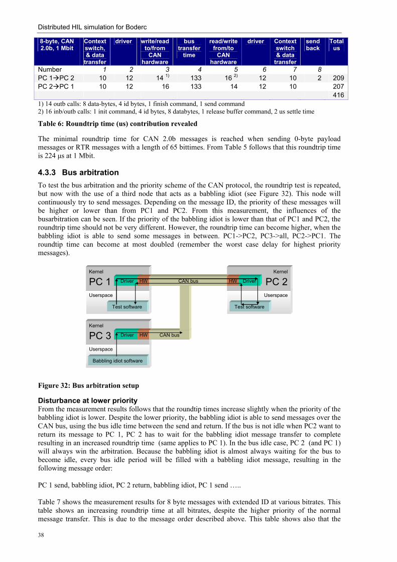
Distributed HIL simulation for Boderc
38
8-byte, CAN 2.0b, 1 Mbit
Context switch, & data
transfer
driver write/read to/from
CAN hardware
bus transfer
time
read/write from/to
CAN hardware
driver Context switch & data
transfer
send back
Total us
Number 1 2 3 4 5 6 7 8 PC 1 PC 2 10 12 14 1) 133 16 2) 12 10 2 209 PC 2 PC 1 10 12 16 133 14 12 10 207 416 1) 14 outb calls: 8 data-bytes, 4 id bytes, 1 finish command, 1 send command 2) 16 inb/outb calls: 1 init command, 4 id bytes, 8 databytes, 1 release buffer command, 2 us settle time
Table 6: Roundtrip time (us) contribution revealed
The minimal roundtrip time for CAN 2.0b messages is reached when sending 0-byte payload messages or RTR messages with a length of 65 bittimes. From Table 5 follows that this roundtrip time is 224 µs at 1 Mbit.
4.3.3 Bus arbitration To test the bus arbitration and the priority scheme of the CAN protocol, the roundtrip test is repeated, but now with the use of a third node that acts as a babbling idiot (see Figure 32). This node will continuously try to send messages. Depending on the message ID, the priority of these messages will be higher or lower than from PC1 and PC2. From this measurement, the influences of the busarbitration can be seen. If the priority of the babbling idiot is lower than that of PC1 and PC2, the roundtrip time should not be very different. However, the roundtrip time can become higher, when the babbling idiot is able to send some messages in between. PC1->PC2, PC3->all, PC2->PC1. The roundtip time can become at most doubled (remember the worst case delay for highest priority messages).
Kernel
Userspace
Driver
Babbling idiot software
HW CAN busPC 3
Kernel
Userspace
Driver
Test software
HW CAN bus HW
Userspace
Kernel
Driver
Test software
PC 1 PC 2
Kernel
Userspace
Driver
Babbling idiot software
HW CAN busPC 3Kernel
Userspace
Driver
Babbling idiot software
HW CAN busPC 3
Kernel
Userspace
Driver
Test software
HW CAN bus HW
Userspace
Kernel
Driver
Test software
PC 1 PC 2Kernel
Userspace
Driver
Test software
HW CAN bus HW
Userspace
Kernel
Driver
Test software
PC 1 PC 2
Figure 32: Bus arbitration setup
Disturbance at lower priority From the measurement results follows that the roundtip times increase slightly when the priority of the babbling idiot is lower. Despite the lower priority, the babbling idiot is able to send messages over the CAN bus, using the bus idle time between the send and return. If the bus is not idle when PC2 want to return its message to PC 1, PC 2 has to wait for the babbling idiot message transfer to complete resulting in an increased roundtrip time (same applies to PC 1). In the bus idle case, PC 2 (and PC 1) will always win the arbitration. Because the babbling idiot is almost always waiting for the bus to become idle, every bus idle period will be filled with a babbling idiot message, resulting in the following message order: PC 1 send, babbling idiot, PC 2 return, babbling idiot, PC 1 send ….. Table 7 shows the measurement results for 8 byte messages with extended ID at various bitrates. This table shows an increasing roundtrip time at all bitrates, despite the higher priority of the normal message transfer. This is due to the message order described above. This table shows also that the

Distributed HIL simulation for Boderc
39
additional roundtrip time is never higher than twice the original roundtrip time, comparable with the worst case delay calculation in section 4.2.4.
Bitrate 100 150 500 1000 average µs 5735 3871 1146 573 max µs 5798 3912 1159 591 min µs 5324 3534 1134 536 average deviation 15.09 9.92 2.94 1.57 std deviation 22.65 16.15 3.73 2.39 average without babbling idiot (µs) 2929 2029 694 415 average difference (µs) 2806 1861 452 158
Table 7: Roundtrip time, 8-byte CAN 2.0b - disturbance at lower priority
Disturbance at higher priority When the babbling idiot sends messages at a higher priority, the situation is the other way around. PC 1 and PC 2 can only start sending their data in the bus idle time of the babbling idiot. Because PC 1 or PC 2 are almost always waiting for the bus to become idle, every bus idle period will be filled with a message, resulting in the following message order: babbling idiot, PC 1 send, babbling idiot, PC 2 return, babbling idiot, PC 1 send ….. The bus idle time for the babbling idiot will be smaller than in the previous case for the normal transfer (no roundtrip ≈ 30 µs). Only at low bitrates (below 150 kbit), PC1 and PC2 get no chance to transfer their messages, because the bus idle time of the babbling idiot is only a few bittimes (1 bittime at 100 kbit = 10 µs). This results in starvation of the normal transfer, because they always loose the bus arbitration. Table 8 shows the results of this measurement. The results from 150 to 1000 kbit/s are similar to the previous case, only at bitrates below 150 kbit, the roundtrip times of the normal message transfer increase dramatically.
Bitrate 100 150 500 1000 average µs 931825 3872 1147 573 max µs 1334195 3920 1230 584 min µs 728475 3632 1064 562 average deviation (µs) 142941 10.52 3.19 1.59 std deviation(µs) 185407 15.04 5.68 2.14
Table 8: Roundtrip time, 8-byte CAN 2.0b - Disturbance at higher priority
4.3.4 Verification & conclusions
Message length & bitstuffing The difference in message length between CAN 2.0a and b were calculated as 19 bits. The measurement results confirm this difference (see Figure 26). The maximum message length seen during the various measurements was 147 bits for CAN 2.0b and 124 bits for CAN 2.0a. These values are lower than the calculated maxima in section 4.2.3, because the chance of having the maximum number of bitstuffing bits is very small.
Protocol overhead & I/O overhead Figure 28 shows the effective bitrate for CAN 2.0b, which is on average 45% of the CAN bitrate. This bitrate includes not only the protocol overhead but also the software overhead. A correction for the software overhead can be made by using the software times from Table 6. The new effective bitrate for this 45% will become:
70.013320745.0 =×
or 70%. This results in a protocol overhead of 30%. The theoretical value for a message lenght of 133 bits is (133-64-29)/133 = 30% which is the same.

Distributed HIL simulation for Boderc
40
The measurement results revealed an important disadvantage of the SJA1000 CAN controller: its single message transmit buffer. A CAN node with this controller can never utilize 100% of the bus time.
Comparison with other measurements A comparison of the roundtrip time measurements with the results from Parchomov (2002) shows similar results. The average values from Table 5 are only a few µs higher as the results with the I+Me Actia board which also uses a SJA1000 controller. Those tests were performed on microcontroller hardware and under Windows with CAN boards from a different vendor. Apparently is the influence of the OS on the roundtrip times limited.
Disturbance at different priority The bus arbitration test indicates a good working priority system, but in combination with bus idle time between two high priority messages, the priority scheme does not work very well. The bus arbitration on message priority works only during the arbitration field. After the arbitration field, the message transfer cannot be cancelled anymore by higher priority messages. To prevent this kind of behaviour, a suitable busscheduling scheme has to be used on top of the priority scheme. E.g.TT-CAN, Hybrid bus scheduling, token based scheduling and timed token based scheduling. Appendix IX describes these busscheduling schemes in more detail.
CAN in the control loop Comparing the results of the roundtrip time measurements and the babbling idiot measurements, it can be concluded that the CAN bus can be used within a control loop if the following conditions are satisfied:
• Sampling time of the control loop > worst case roundtrip time • Only one bidirectional CAN transfer in the control loop • Highest priority for the CAN message transfer in the control loop
The babbling idiot test shows that the normal roundtrip time increases at most with a factor two when other CAN nodes interfere with the control loop transfer. Example For an 8-byte extended id CAN transfer at 1 Mbit, the maximum roundtrip time is 428 µs. The sample frequency of the control loop can be at most 2 kHz under the assumption that the calculations are fast and that the bus is not shared with other (non controller) nodes. In case, the bus is shared, the maximum roundtrip time should be doubled, which results in a maximum sample frequency of 1 kHz.


Distributed HIL simulation for Boderc
42

Distributed HIL simulation for Boderc
43
5 Communicating Threads
5.1 Introduction A number of extensions (mainly linkdrivers) are needed in order to use the CT library (Hilderink, G.H., 1997) together with the ECS setup hardware. This chapter describes the issues involved in running CT programs under Linux and the linkdrivers written for the ECS CAN hardware and the Anything I/O board. Some of the linkdrivers require modifications of the CT kernel in order to work under Linux. These changes are also described here.
5.2 CT internals The CT library provides non-preemptive priority-based scheduling for multiple threads of execution (=CT processes) inside an event driven application. All processes run in the same address space of the application. Each process has its own individual program counter and run-time stack and may contain private variables (a process is a running instance of a class and can therefore contain private variables) and public variables. CT is a userspace threading library, which means that all CT threads run inside a single operating system thread. The process scheduling under CT is done in a cooperative way. The processes are managed and dispatched by a priority- and event-driven based non-preemptive scheduler. The PriPar and PriAlt construct determine the scheduling priority and the channel communication can be seen as an event. The event-driven scheduling allows processes to wait until they can participate in a communication event. Use of long running processes that do not communicate via channels should be prevented or should contain manual reschedule calls (thread yield) due to the non preemptive scheduler. Scheduling in a CT program is hidden by the channels and is a part of the program, not the OS.
5.3 Linkdriver concept As described in the introduction chapter, all processes communicate with each other using channels. Besides normal (internal memory) channels, processes can also communicate via channels to hardware or via some communication link with remote processes. For this channel communication, the channel object needs a driver to communicate with the hardware. These drivers are called linkdrivers and can be inserted into the build-in channels. The processes itself are hardware (and platform) independent. The linkdrivers take care of the underlying hardware communication. Figure 33 illustrates the linkdriver concept for a remote channel between process A and B (Hilderink, G.H. et al., 2000).
Figure 33: CT linkdriver concept for remote channels
5.3.1 Extended linkdriver concept The current linkdriver concept assumes point-to-point communication and supports only one channel over a physical communication link, because channels have no support for addressing. Different options exist to support multiple channels over one physical like the CAN bus. The first option uses multiple instances of a linkdriver concurrently accessing the fieldbus hardware. In principle this could work, but at the receiving side arises an addressing problem. The CAN

Distributed HIL simulation for Boderc
44
hardware reads a message from the bus and one of the linkdrivers will read it. It is not possible to to predict which of the linkdrivers will read the message and it is also not possible to send a message to a specific linkdriver. The problems here are the concurrent hardware access and the lack of addressing capabilities to connect the correct channel ends to each other.
Figure 34: One linkdriver per channel
A second option is to use channel multiplexing using the scheme presented in Figure 35. With this structure, only one linkdriver is required and the problem of the concurrent hardware access is gone. Here processes S and F play the role of channel multiplexer and demultiplexer. S forwards the data from al its incoming channels over one single output channel.
Figure 35: Multiplexing using a CT process and 1 linkdriver
A problem with this configuration is still the addressing of the processes. If process F receives a message from P via S, F does not know for which of the processes (C, D, E) this message is intended, because CT processes do not know each other. Somehow P should inform F that the data F receives from S is intended for process C. P does not know that C is on a remote target because it does not know C at all. So P cannot add an address to its message. The multiplexer process S does know the different source channels and can add a source channel number to each message but how does F know which of the three destination channels corresponds to the channel number inside the received message? This is only possible by using a fixed channel order on both sides in the processes S and F. Consequently, these processes need to be changed whenever the distributed structure of the CT processes change, which is not flexible. The third option is similar to the second option, but the multiplexing/demultiplexing does not occur inside a CT process, but in an intermediate object between the linkdriver and the CAN bus, which inserts some content addressing. Extra options, like sending acknowledgment messages and achieving fault tolerant communication can also be implemented using this extended linkdriver framework. An implementation of this extended linkdriver framework is already available for the C version of the CT library. See (Orlic et al., 2003)) for more information.
P
Q
R
C
D
E
Linkdriver 1
Linkdriver 2
Linkdriver 3
Linkdriver
P
Q
R
S
C
D
E
F

Distributed HIL simulation for Boderc
45
Figure 36: Extended linkdriver framework
This extended linkdriver framework will be used for the implementation of the TCP/IP linkdriver and the CAN linkdriver, discussed in the next section.
5.4 Linkdrivers written for the Boderc project All described linkdrivers below, are written under Linux and only useable under Linux. DOS/Windows versions are not planned because they lie outside the scope of this project.
5.4.1 TCP/IP socket linkdriver
Introduction The purpose of the TCP socket linkdriver was to get familiar with the CT linkdriver concept. The TCP/IP linkdriver is used to test a major part of the CAN linkdriver code (described below). The advantage of the TCP socket linkdriver compared to the CAN linkdriver is that it can be tested on every Linux PC even without a network adapter. Furthermore, this linkdriver can be used for fall back channels in case of a CAN link failure or to exchange logging data between the ECS pc’s and the development machine.
Implementation The TCP/IP socket linkdriver uses the socket IPC (Inter Process Communication) mechanism found on many Unix and Windows machines. Sockets are a very general mechanism that accommodates many different network protocols. Because each IP datagram is send separately, possibly over different routes, to its destination, the IP service cannot guarantee that all packets will arrive in the same order as they were send, or even that they will arrive at all. The User Datagram Protocol (UDP) adds communication ports to the IP protocol, providing multiple communication channels over the network. Using this port scheme, incoming messages can be delivered to the right process (e.g. a web server). This process can also reply to the originating process. The UDP protocol uses the IP protocol to transfer messages and therefore, it has the same unreliable connectionless message transfer. To get a more reliable transfer with error detection and correction mechanisms, re-ordering and guaranteed data arrival, the TCP protocol can be used on top of the IP protocol. The TCP protocol is a connection based protocol providing a connection between two fixed processes (using ports, just like UDP). For the socket linkdriver the TCP/IP was chosen over UDP because of the error detection/correction and retransmission. The linkdriver uses internally the common BSD/Unix socket system calls like connect, listen, accept, read/write.
Results The Linux TCP/IP socket linkdriver is implemented as a rendezvous channel. The linkdriver is able to create CSP channels for all C++ data types, including user-defined data types in structures. It uses the
P
Q
R
DeviceD
river Dev
iceD
river
RemoteLinkdriver 1
RemoteLinkdriver 2
RemoteLinkdriver 3
C
D
E
RemoteLinkdriver 1
RemoteLinkdriver 3
RemoteLinkdriver 3

Distributed HIL simulation for Boderc
46
basic ideas of the extended linkdriver framework by Orlic (2003), to create more than one channel over one single socket link. Fault tolerance9 using a backup link (Orlic et al., 2003) is not supported but can be implemented in the future if needed. More about the implementation of the extended linkdriver framework can be found in the CAN linkdriver section. The rendezvous mechanism is implemented by sending Ack messages for every received message. These Ack messages are send just before the CT channel gets the received data. It is also used for synchronization purposes between two distributed processes connected to each other via a remote channel (in this case, a TCP/IP channel). It is impossible to get an exact time synchronization, between the two remote processes, because the receiver will continue after the transmission of the Ack and the sender just after the reception of the Ack. The time required for the transmission is also the time difference between both synchronization points.
Implementation issues and remarks • When a program wants to read data from a socket (or in general, from a file) and no data is
available, the Linux read() function blocks the current Linux thread until data is available. If a CT program uses the same read() function, the entire CT program is blocked, not only the calling process. The CT threads are hidden for Linux. So the Linux kernel assumes that it can suspend the current Linux thread on a blocking system call like read() until this system call is finished. As a consequence, other parallel processes stop running. This is not the intended behaviour.
Figure 37: CT threads ‘hidden’ in one Linux thread
This problem is depicted Figure 37, where the first thread is suspended due to the blocking system call.(1). The Linux kernel (2) transfers the thread execution to the next Linux thread (3). It is possible to solve this by using a non-blocking (O_NONBLOCK) read(). The CT program will then continue when no data is available. But now, the program needs to poll for data availability in regular intervals. Normally, the Linux Select and Poll functions are a suitable solution for the polling, but also these functions block the entire CT program until data is available or until a timeout occurs. For now, the TCP/IP linkdriver uses the standard Linux read/write commands in non-blocking mode. To check if data is available or if data can be written on the socket link, the linkdriver uses a polling mechanism (busy waiting). A possible solution to prevent this busy waiting is to extend the CT library with a system call wrapper facility for read, write, select and poll in the same way as used in the GNU Portable Threads library (Engelschall, 2003).
• The TCP socket linkdriver provides only multiple point to point connections. For each connection from one target to another, a new remote linkdriver object has to be created. Multiple channels directed to the same target platform can use the same TCPIPDeviceDriver object by sharing one
9 Part of the extended linkdriver framework
Linux thread 1
CT
Proc
ess
1
CT
Proc
ess
2
CT
Proc
ess
3
Linux kernel
Linux thread 2
systemcall 1
2
3
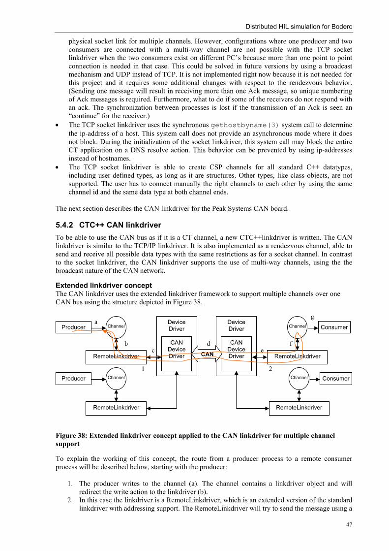
Distributed HIL simulation for Boderc
47
physical socket link for multiple channels. However, configurations where one producer and two consumers are connected with a multi-way channel are not possible with the TCP socket linkdriver when the two consumers exist on different PC’s because more than one point to point connection is needed in that case. This could be solved in future versions by using a broadcast mechanism and UDP instead of TCP. It is not implemented right now because it is not needed for this project and it requires some additional changes with respect to the rendezvous behavior. (Sending one message will result in receiving more than one Ack message, so unique numbering of Ack messages is required. Furthermore, what to do if some of the receivers do not respond with an ack. The synchronization between processes is lost if the transmission of an Ack is seen an “continue” for the receiver.)
• The TCP socket linkdriver uses the synchronous gethostbyname(3) system call to determine the ip-address of a host. This system call does not provide an asynchronous mode where it does not block. During the initialization of the socket linkdriver, this system call may block the entire CT application on a DNS resolve action. This behavior can be prevented by using ip-addresses instead of hostnames.
• The TCP socket linkdriver is able to create CSP channels for all standard C++ datatypes, including user-defined types, as long as it are structures. Other types, like class objects, are not supported. The user has to connect manually the right channels to each other by using the same channel id and the same data type at both channel ends.
The next section describes the CAN linkdriver for the Peak Systems CAN board.
5.4.2 CTC++ CAN linkdriver To be able to use the CAN bus as if it is a CT channel, a new CTC++linkdriver is written. The CAN linkdriver is similar to the TCP/IP linkdriver. It is also implemented as a rendezvous channel, able to send and receive all possible data types with the same restrictions as for a socket channel. In contrast to the socket linkdriver, the CAN linkdriver supports the use of multi-way channels, using the the broadcast nature of the CAN network.
Extended linkdriver concept The CAN linkdriver uses the extended linkdriver framework to support multiple channels over one CAN bus using the structure depicted in Figure 38.
Figure 38: Extended linkdriver concept applied to the CAN linkdriver for multiple channel support
To explain the working of this concept, the route from a producer process to a remote consumer process will be described below, starting with the producer:
1. The producer writes to the channel (a). The channel contains a linkdriver object and will redirect the write action to the linkdriver (b).
2. In this case the linkdriver is a RemoteLinkdriver, which is an extended version of the standard linkdriver with addressing support. The RemoteLinkdriver will try to send the message using a
Producer Channel
RemoteLinkdriver
Device Driver
CAN Device Driver
Producer Channel
RemoteLinkdriver
ConsumerChannel
RemoteLinkdriver
Device Driver
CAN Device Driver
CAN
ConsumerChannel
RemoteLinkdriver
a
b c
de
f
g
1 2

Distributed HIL simulation for Boderc
48
DeviceDriver (in this case a CANDeviceDriver) (c). If the DeviceDriver cannot send the message, the RemoteLinkdriver will block the channel write (a) and CT schedules to another process. If the DeviceDriver is able to send the message, the RemoteLinkdriver continues, waiting on a acknowledgment message (for rendezvous behaviour).
3. The CANDeviceDriver sends the message including the unique address from the RemoteLinkdriver over the CAN bus to the remote side (d). The unique address is used as the identifier field of the CAN message.
4. The CANDeviceDriver at the remote side receives the message from the CAN bus, reads the unique address and searches the corresponding RemoteLinkdriver in a lookup table. The message will be put (e) in an internal buffer inside the RemoteLinkdriver until the Consumer wants to read from its channel (g).
5. If the consumer starts reading from its channel (g), the RemoteLinkdriver (2) read is invoked via (f) and the message will be retrieved from the internal buffer.
6. At the same time, the RemoteLinkdriver (2) sends an acknowledgement message to its DeviceDriver via (e).
7. This acknowledgement message is returned via (d) and (c) to the RemoteLinkdriver (1), which will unblock the channel (rendezvous communication is completed), so that the producer can continue its work.
Timing in CT? The RemoteLinkdriver class has a build-in time-out feature to prevent a deadlock situation when the acknowledge message never arrives. Because the Linux version of CTC++ has currently no timing support, it not possible to generate the timeout event using the CT library. Therefore, a set of alarm functions is written to make it possible to wake-up a CT process after a specified time-out. It uses a timer callback function inside the the RemoteLinkdriver to wake-up the linkdriver. So, a locked RemoteLinkdriver object can be unlocked via a timeout event or by the arrival of data. If the data arrives within 1 second, the request for a timeout will be cancelled. The alarm functions use the Linux alarm() function and the SIGALARM signal to call the TimerCallback function. The timeout accuracy is 1 second. Listing 3 shows a stripped version of the used C++ code inside the RemoteLinkdriver to generate the timeout. RemoteLinkdriver.h Class RemoteLinkdriver: public LinkDriver, public TimerCallback { … Timercallback(void); //wake-up for time-outs generated by the timer class … } RemoteLinkdriver.cpp RemoteLinkdriver::Timercallback(void) { timeout=true; unlock(); } RemoteLinkdriver::write(Object object, unsigned int size) { … {Normal write stuff} … //Wait for acknowledgement message timeout=false; add_alarm(this,1); //Wake me up at t+1 (in seconds) lock(); //Unlock via ack arrival or time-out if (timeout==false) remove_alarm(this); //Cancel time-out wakeup … } TimerCallback.h class TimerCallback { public: virtual void timercallback(void) = 0; //Only specify the required function call //every process that inherits this class must contain its own timercallback function };

Distributed HIL simulation for Boderc
49
ct-time.cpp void init_alarm(void); //Inform CT kernel about SIGALRM use void catch_alarm (int sig); //signalhandler for SIGALRM void add_alarm (TimerCallback* processptr, int wakeup_after_sec); //Add alarm to the queue void remove_alarm (TimerCallback* processptr); //Remove alarm from the queue
Listing 3: Time-out implementation in the RemoteLinkdriver
This time-out solution is working, but it is recommended to search for better timing solution that can be implemented in CT. E.g. one standard Timer object/process that handles all timing inside a CT program. That process should handle all sleep, suspend and other time related functionality.
Blocking problem During the implementation of this communication concept, it became clear that the CAN linkdriver has the same blocking problem as occurred with the TCP/IP linkdriver. For the TCP/IP linkdriver, it was solved by ignoring the problem and using polling to check for data availability. Because the blocking problem is a serious problem under Linux (and Windows) in combination with CT and devicedriver or file access, a solution needs to be found. Below, some possible solutions will be investigated. Possible solutions:
1. The CAN card generates interrupts when sending and receiving data. It would be useful to use these interrupts in combination with lock() and unlock() to block a CT process on a channel while other CT processes keep running. This would work under DOS, but under Linux, an additional handicap exists. It is not possible to access hardware interrupts from user space programs. Only the CAN kernel module can handle these interrupts. Somehow, this module has to inform the CT user space program that data is available. This can be done using signals (software interrupts).
2. Do the blocking read in a second PThread/Linux thread, outside the CT processes. 3. Alter CT in such a way that it offers “own” read and write function calls that block only
reading/writing CT process. The latter solution is also used by the by the GNU Portable Threads library (Engelschall, 2003), another user space thread library, like CT, but based on the traditional way of thread programming like using PThreads.
4. Rewrite CT to use operating system threads (when running under an operating system) instead of its own threading mechanism, keeping its own scheduler
The first solution is possible for the CAN linkdriver, by altering the CAN kernel driver. Some additional code is required that generates a signal inside the IRQ handler, to unlock a CAN channel. This solution has some disadvantages. It cannot be used for the TCP/IP linkdriver. Other disadvantages of the signals solution are that Linux cannot guarantee that every individual signal send to a process will be delivered (GNU, 2001). If multiple signals of the same type are delivered to a process before the processes signal handler has a chance to be invoked, the handler may only be invoked once, as if only a single signal had arrived. For the process, the signals merge into one. The most common situation in which this can happen is when a signal is blocked or when the system is running other processes. So, it is not reliable to use a signal handler to count messages. If the CAN kernel module sends a signal for every message it receives, the CT program still needs to check if more data is available after reading the first message, because the signal could be a merged one (GNU, 2001). The second solution, using a separate non-CT thread that will do the blocking system calls, seems a better solution, because it is also useable for the TCP/IP linkdriver and it can be implemented without any changes to CT. During the implementation, it turned out that the cooperation between the CTC++ library and PThreads/Linux threads currently is not possible. Using PThreads in combination with CT does not work well because of conflicting stack changes when calling Linux system calls. This gives undefined stack contents and will generate segmentation faults. Because the second solution did not work, some other Linux multithreading libraries were tested, mostly with the same segmentation faults. One of these libraries is the PortableThreads library (GNU Pth, open source (Engelschall, 2003)). The authors of this user space threading library faced the same

Distributed HIL simulation for Boderc
50
blocking problems and they have found a solution. The Pth library has implemented a set of wrapper functions for read, write, ioctl, select and poll that will internally block only the calling Portable thread. From the Linux point of view, they use non blocking in combination with a central event manager that will keep an eye on the I/O status. If data becomes available, the event manager will unblock the calling Portable thread, simulating a standard blocking system call. This solution would be a good extension of the Linux version of the CT library. However, this solution requires a major adaptation of CT and it is more difficult to implement that the other solutions. The fourth solution requires also a major adaptation of CT. The CT kernel needs to be changed to use operating system threads under Linux. This adaptation has a main drawback. The difference in context switch times between two threads in CT and with PThreads large. Context switch times for kernel threads are much higher than for userspace threads. See Table 9 for the results of a context switch test for the different threading libraries. This test is performed by letting two threads continuously switch between each other during one minute. CT Pth PThreadsContext switches per minute 75 774 799 431 702 708 119
Table 9: Context switches per minute under Linux at 2.4 GHz Pentium 4
The first solution, using signals, was chosen for the implementation of the CAN linkdriver, despite its disadvantages. The CAN linkdriver uses a modified version of the Linux CAN device drivers from Peak System10 and can be used only under Linux. The changes will be described below. To cope with merged signals, the signal handler in the CAN linkdriver checks for additional messages after receiving the first one. The receive signalhander inside the CAN linkdriver is aware of merging signals. At the end of the signalhandler, the linkdriver checks for new messages received while processing the message that caused the signal. The signals used for the CAN linkdriver are asynchronous signals. The signals can arrive on every moment, even while the process is currently running the signal handler for that signal. Linux will automatically block this second signal until the first signal has been handled. A different kind of signal may still interrupt the handling of a signal. Normally, one would use signal to handle signals. For the asynchronous signals, this is not a good choice, because one needs to re-establish the signal handler each time it runs. If a second signal arrives just before the signal handler is re-established again, this signal will run the default handler and may terminate the process. Using sigaction is a solution to prevent this kind of behaviour. Therefore, the CAN linkdriver uses sigaction to install its signalhandlers.
Changes to CT with respect to signals During the implementation of the CAN linkdriver, it turned out that the Linux version of the CT library had no support for atomic regions using enterAtomic/exitAtomic. These functions are available but normally they only disable (hardware) interrupts. Under Linux, normal (user space) programs cannot access interrupts, so these functions have no effect. However they should block signals (software interrupts). It turned out that signals arrive within the ‘atomic’ region defined by enterAtomic/exitAtomic. To prevent this behavior, the enterAtomic/exitAtomic functions are altered to disable signals under Linux. Because disabling/enabling signals will take some additional time (around 1 µs), the modified CT kernel currently uses a Processor__add_signal function to tell which signals should be disable under Linux inside an atomic region. If no signals are used or CT is not informed about the used signals/signalhandlers, signals will not be disabled/enabled by any enterAtomic/exitAtomic pair. Only the Linux and Linux-uClibc version of the CTC(PP) library contain these changes. With these modifications a CT program that uses signals, does not end with segmentation fault anymore if a signal arrives during a context switch.
10 The CAN boards are from the company Peak System.

Distributed HIL simulation for Boderc
51
Altered CAN kernel module To be able to generate signals at the arrival of an interrupt, the CAN kernel module had to be modified. The altered CAN kernel module is compatible with the standard CAN module11 from Peak System, except for the differences mentioned below: Differences • No support for PCAN Dongle and PCAN USB devices • kernel module sends SIGUSR1 signals at data arrival • kernel module sends SIGUSR2 signals at bus ready for writing To use the modified kernel module also with other non-CT programs, like the delivered test utilities, the kernel module will not generate any signals on an interrupt, until the application informs the kernel module that it is able to handle the signals. Otherwise, the program will terminate unexpectedly caused by an unhandled signal. Figure 39 shows the structure of the CAN linkdriver with signals.
Figure 39: Overview of the Linux CAN linkdriver for the Peak System boards
The signal solution works as follows: 1. The CANDeviceDriver (1) uses non-blocking I/O to send it message to the kernel driver (a). 2. The kernel driver (2) sends the message over the CAN bus (b) to the remote side (3). 3. The other kernel driver (3) receives a “receive” interrupt from the CAN hardware and it starts
reading the message into its FIFO buffer. The kernel driver sends a SIGUSR1 signal (c) to the CANDeviceDriver (4) to inform it about the data arrival.
4. The signalhandler of the CANDeviceDriver reads the message from the kernel module (d) and sends it to the correct RemoteLinkdriver (e)
Of course, this picture would be a lot simpler when the entire CT program is transferred to kernel space. At first, this would be the best solution. Drawback is that the kernel has no C++ support, limiting the use of the CT library to the CTC version. CTC++ code is object oriented and better readable than the pseudo object oriented code from CTC.
CTC++ Example Listing 4 shows an example for the declaration of a consumer and a producer process that communicate with some remote processes via two CAN channels.
11 Version 1.40 of the Linux drivers was used as basis for the altered drivers.
User space
Kernel space
User space
Kernel space
Producer Channel
RemoteLinkdriver
Device Driver
CAN Device Driver
ConsumerChannel
RemoteLinkdriver
Device Driver
CAN Device Driver
PeakCAN kernel
module
PeakCAN kernel
module
SIGNAL
CAN
SIGNAL
1
2
4
c3
b
a d
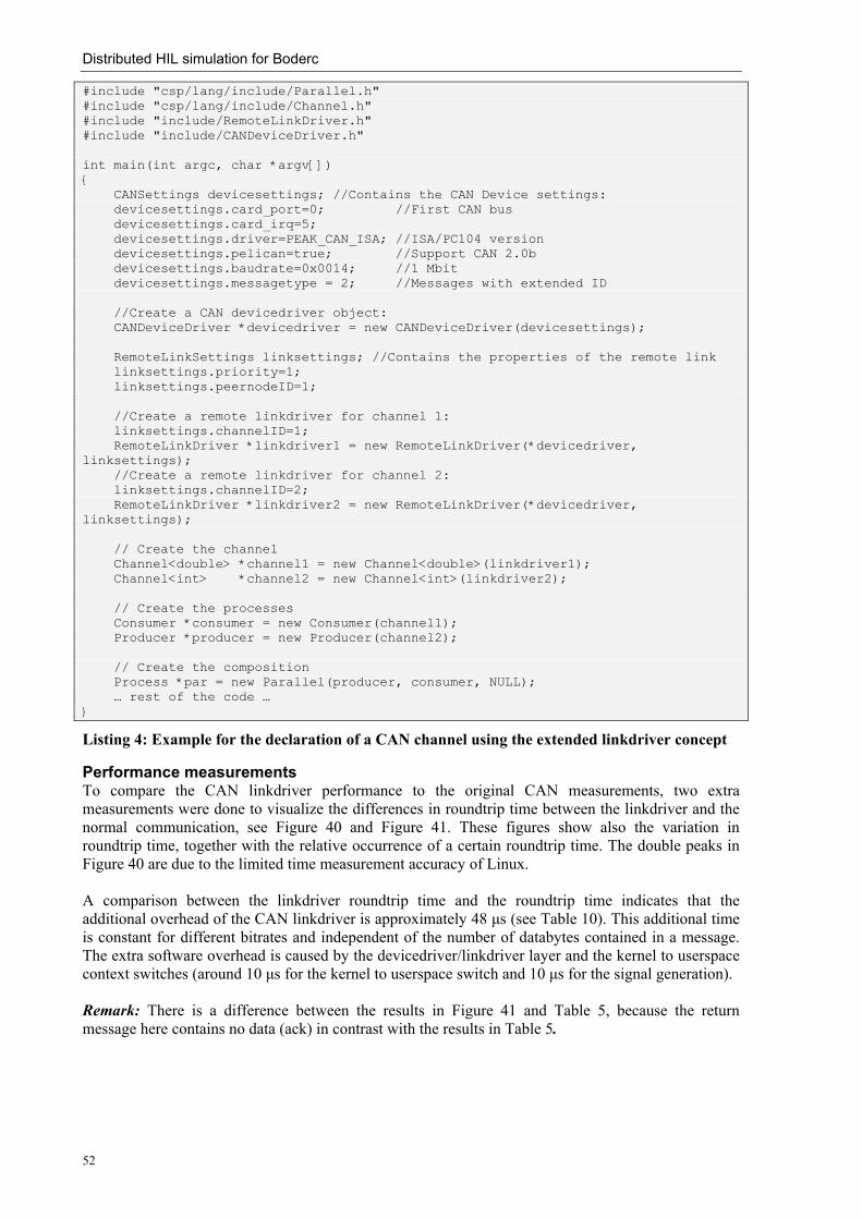
Distributed HIL simulation for Boderc
52
#include "csp/lang/include/Parallel.h" #include "csp/lang/include/Channel.h" #include "include/RemoteLinkDriver.h" #include "include/CANDeviceDriver.h" int main(int argc, char *argv[]) { CANSettings devicesettings; //Contains the CAN Device settings: devicesettings.card_port=0; //First CAN bus devicesettings.card_irq=5; devicesettings.driver=PEAK_CAN_ISA; //ISA/PC104 version devicesettings.pelican=true; //Support CAN 2.0b devicesettings.baudrate=0x0014; //1 Mbit devicesettings.messagetype = 2; //Messages with extended ID //Create a CAN devicedriver object: CANDeviceDriver *devicedriver = new CANDeviceDriver(devicesettings); RemoteLinkSettings linksettings; //Contains the properties of the remote link linksettings.priority=1; linksettings.peernodeID=1; //Create a remote linkdriver for channel 1: linksettings.channelID=1; RemoteLinkDriver *linkdriver1 = new RemoteLinkDriver(*devicedriver, linksettings); //Create a remote linkdriver for channel 2: linksettings.channelID=2; RemoteLinkDriver *linkdriver2 = new RemoteLinkDriver(*devicedriver, linksettings); // Create the channel Channel<double> *channel1 = new Channel<double>(linkdriver1); Channel<int> *channel2 = new Channel<int>(linkdriver2); // Create the processes Consumer *consumer = new Consumer(channel1); Producer *producer = new Producer(channel2); // Create the composition Process *par = new Parallel(producer, consumer, NULL); … rest of the code … }
Listing 4: Example for the declaration of a CAN channel using the extended linkdriver concept
Performance measurements To compare the CAN linkdriver performance to the original CAN measurements, two extra measurements were done to visualize the differences in roundtrip time between the linkdriver and the normal communication, see Figure 40 and Figure 41. These figures show also the variation in roundtrip time, together with the relative occurrence of a certain roundtrip time. The double peaks in Figure 40 are due to the limited time measurement accuracy of Linux. A comparison between the linkdriver roundtrip time and the roundtrip time indicates that the additional overhead of the CAN linkdriver is approximately 48 µs (see Table 10). This additional time is constant for different bitrates and independent of the number of databytes contained in a message. The extra software overhead is caused by the devicedriver/linkdriver layer and the kernel to userspace context switches (around 10 µs for the kernel to userspace switch and 10 µs for the signal generation). Remark: There is a difference between the results in Figure 41 and Table 5, because the return message here contains no data (ack) in contrast with the results in Table 5.
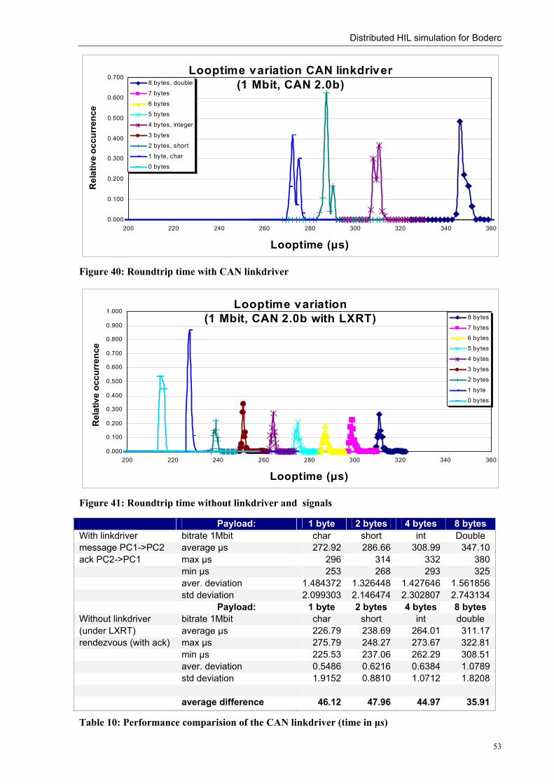
Distributed HIL simulation for Boderc
53
Looptime variation CAN linkdriver(1 Mbit, CAN 2.0b)
0.000
0.100
0.200
0.300
0.400
0.500
0.600
0.700
200 220 240 260 280 300 320 340 360
Looptime (µs)
Rel
ativ
e oc
curr
ence
8 bytes, double
7 bytes
6 bytes
5 bytes
4 bytes, integer
3 bytes
2 bytes, short
1 byte, char
0 bytes
Figure 40: Roundtrip time with CAN linkdriver
Looptime variation(1 Mbit, CAN 2.0b with LXRT)
0.000
0.100
0.200
0.300
0.400
0.500
0.600
0.700
0.800
0.900
1.000
200 220 240 260 280 300 320 340 360
Looptime (µs)
Rel
ativ
e oc
curr
ence
8 bytes
7 bytes
6 bytes
5 bytes
4 bytes
3 bytes
2 bytes
1 byte
0 bytes
Figure 41: Roundtrip time without linkdriver and signals
Payload: 1 byte 2 bytes 4 bytes 8 bytes With linkdriver bitrate 1Mbit char short int Double message PC1->PC2 average µs 272.92 286.66 308.99 347.10 ack PC2->PC1 max µs 296 314 332 380 min µs 253 268 293 325 aver. deviation 1.484372 1.326448 1.427646 1.561856 std deviation 2.099303 2.146474 2.302807 2.743134 Payload: 1 byte 2 bytes 4 bytes 8 bytes Without linkdriver bitrate 1Mbit char short int double (under LXRT) average µs 226.79 238.69 264.01 311.17 rendezvous (with ack) max µs 275.79 248.27 273.67 322.81 min µs 225.53 237.06 262.29 308.51 aver. deviation 0.5486 0.6216 0.6384 1.0789 std deviation 1.9152 0.8810 1.0712 1.8208 average difference 46.12 47.96 44.97 35.91
Table 10: Performance comparision of the CAN linkdriver (time in µs)

Distributed HIL simulation for Boderc
54
The CAN linkdriver is also tested under LXRT12/RTAI, but this has no effect, due to two reasons: within LXRT hard-real-time, it is not possible to use signals and besides that, the PCAN kernel driver is not RTAI compatible (RTAI enforces some restrictions to assure real-time behaviour). Both cause LXRT to return to the soft real-time mode, which is the same as a normal highest priority process under Linux. Also a stress test was done (reading the entire flashdisk) during the CAN communication experiment. Under RTAI, this should not influence the CAN communication. During this test, the roundtrip times varied much more (standard deviation was more than 16 times higher), which is not useable for hard real-time communication. Conclusion is that the current CAN driver & linkdriver are not useable in a hard real-time environment like RTAI offers. Main cause is the PCAN driver, which is not RTAI compatible. The current CAN linkdriver is useable in a control loop, because the roundtrip results under normal circumstances are stable enough, on the condition that the system is not overloaded. The PCAN driver should be ported to RTAI to make the linkdriver behaviour more stable during overload conditions.
5.4.3 Digital I/O linkdrivers This section will describe the written linkdrivers that provide I/O channels to CT on the PC/104 PC’s.
Parallel port linkdriver A simple (Linux only) linkdriver was written to access the parallel port hardware using channels. The linkdriver will accept bytes and bits or in CT terminology: Channel<char> and Channel<bool>. The parallel port linkdriver can be used to provide some basic I/O possibilities to a CT program on a normal PC without dedicated I/O hardware. The parallel port is, for example, used for the CAN communication measurements, to signal the start and end point of a read and a write action. Together with an oscilloscope that triggers on the beginning of a CAN message, one can measure exactly how much time is spent on different software and hardware parts. See section 4.3 for these results. Listing 5 gives a small CTC++ example for the declaration of a parallel port channel. All required settings for the parallel port channel are embedded into a struct with the name ParPort_settings. The devicenumber ranges from 1 to 3 and corresponds with LPT1 to LPT3. The offset option is optional, but can be used to write/read to/from the LPT status register (offset =1) or the LPT control register (offset=2). The bitoffset option (optional) can be used for Boolean (bit) channels to specify the LPT pinnumber that needs to be controlled. Currently this linkdriver required root access under Linux to access the required I/O registers. This can be prevented in the future by adding support for the standard Linux way for parallel port access, using /dev/parport. // Include the ParPort linkdriver include file #include "include/ParPort.h" //Settings for this parallel port channel: ParPort_settings settings; settings.devicenr = 1; //1=LPT1, 2=LPT2, 3=LPT3 settings.offset = 0; //0=data register(o), 1=status(i), 2=control (i/o) settings.bitoffset = 0; //0=D0 to 7=D7 for Channel<bool> settings.direct_io = true; //Create the ParPort I/O linkdriver channel (datatype = Channel<bool>) Channel<bool> *channel = new ParPort(&settings); //Use the channel: Producer *producer = new Producer(channel); //Accepts Channel<bool>
Listing 5: Example code for using the parallel port linkdriver
12 LXRT is the userspace extension of RTAI, which allows userspace programs to run in a hard-real-time environment. Standard RTAI programs are kernel modules.
Distributed HIL simulation for Boderc
55
Remark: Sometimes, it can be useful to write to the data register (offset=0) and read back some status information from the status register (offset=1). Due to the different offset valus, this would be impossible with one channel. This is solved by adding a feature to the ParPort-channel read function. One can pass the read offset at runtime to the read function by placing the required offset into the read buffer. After the read action, this buffer will contain the data read from the I/O register indicated by the offset. data = 255; parportchannel->write(&data); //Write to data register data = 1; parportchannel->read(&data); //Read from status register (offset = 1)
5.5 Anything I/O linkdrivers
5.5.1 Introduction To communicate with the Anything I/O board connected to the PC/104 stack, one or more I/O linkdrivers are required to access the I/O hardware from a CT process. Normally, the linkdriver structure delivers a convenient way to hide hardware access into a channel. This is also possible for the Anything I/O board, but there is a problem. The onboard FPGA can be programmed with many completely different hardware configurations. Each configuration has its own register map and port addresses. It not possible to write one general purpose linkdriver that can be used for all hardware configurations. It is possible to write a linkdriver that can read and/or write to every hardware portaddress, but this solves only a part of the problem. Initialisation of the hardware is specific for each FPGA configuration. On one hand, a configuration specific initialization routine is required and on the other hand for the access to specific functions (e.g. PWM or encoders) a general linkdriver can be used, because most of the times, reading and/or writing is nothing more that reading/writing to an I/O port. The simplest way is to write a set of linkdrivers per FPGA configuration. However, there should be some check inside the linkdriver on the current FPGA configuration. Using a linkdriver together with the wrong FPGA configuration will give unpredictable results and may even damage the connected hardware or the FPGA itself. All Anything I/O linkdrivers, described below, check the status and configuration of the FPGA before the hardware initialization. They will only work if the correct FPGA configuration is programmed. There are two options for the detection of the correct hardware configuration:
• via the filename of the programfile • addition of an unique ID to the VHDL code that can be read from a specific I/O register
The first option seems the simplest one. It would work with all compiled FPGA configurations, but there is a small problem. The kernelmodule does not know the filename of the file once copied to the device filesystem. It receives only the data. The .BIT program files contain the original project name (e.g. “hostmot5.ncd”) but the .PROM program files do not contain the name. This option is only useable when .BIT files (default in the Xilinx software) are used. The second option has a disadvange that it requires changes to all currently available hardware configurations. The advanges are that it is now possible to create different configurations with the same ID, allowing the linkdrivers to use both configurations as long as they have a compatible port map. The linkdrivers described below, all use the filename as a configuration check. The linkdrivers can be found in the HIL CVS repository together with a small testprogram.
5.5.2 HOSTMOT5 PWM & encoder linkdrivers To use the functionality provided by the HOSTMOT5 FPGA configuration in CT programs, a library with a set of linkdrivers was written specific for this configuration. The HOSTMOT5 configuration

Distributed HIL simulation for Boderc
56
has 12 pulse width modulation (PWM) outputs with direction pins and 12 A-B encoder inputs with index pins. The library provides an encoder linkdriver and a PWM linkdriver.
Encoder channel linkdriver The encoder channel linkdriver communicates with the Anything I/O driver via the device filesystem as depicted in Figure 21 (3). The encoder channel is a bidirectional channel that accepts long (=DWORD) values. Reading from the channel will return the last known encoder value and writing to the channel will reset the quadrature encoder counter to 0. This linkdriver supports also the direct I/O access backdoor (h, in Figure 21) for faster I/O access. All settings for the linkdriver, like the encoder number, direct I/O and the devicenumber, are contained in one struct variable. Listing 6 contains a short C++ example of the declaration and use of an encoder channel in CTC++. // Include the Anyio linkdriver include file #include "enc/anyio_hostmot5_enc.h" //Encoder channel settings: Anyio_hostmot5_enc_settings encsettings; encsettings.devicenr=0; //0..3 for /dev/anyio0 .. /dev/anyio3 encsettings.enc_port=5; //0..11 for ENCODER0 to ENCODER11 encsettings.direct_io=true; //use direct i/o access if true, else use //kernelmodule for I/O-access //Create an Anything HOSTMOT5 encoder channel (datatype=long) Channel<long> *encchannel = new Anyio_hostmot5_enc(&encsettings); //Create a process Consumer *consumer = new Consumer(encchannel); //Accepts Channel<long>
Listing 6: Example code for declaration of an encoder channel
PWM channel linkdriver The PWM channel linkdriver is similar to the encoder linkdriver. This linkdriver provides access to the PWM and motor direction outputs of the HOSTMOT5 configuration. The PWM channel is a bidirectional channel that accepts singed short (=WORD) values. The sign of the data determines the motor direction. Reading from the channel will return the current PWM value and writing to the channel will alter the PWM duty cycle of the corresponding PWM port. The PWM port has a 12 bit (11 bit data + 1 sign bit) dutycyle, so the first 4 least significant bits do not influence the PWM duty cycle. The linkdriver settings are contained in a struct variable and are similar to the encoder settings. The PWM linkdriver has one additional option for enabling the PWM interlace mode. In this mode, the frequency of the PWM signal is always as high as possible; keeping the average duty cycle the same (see Figure 42). This is useful when using the PWM output (together with a low pass filter) as DA convertor.
Figure 42: Interlaced versus normal PWM
Listing 7 contains a short C++ example of the declaration and use of a PWM channel in CTCPP.
Interlaced PWM
Standard PWM Duty cycle = 50%
Duty cycle ≈ 50%

Distributed HIL simulation for Boderc
57
// Include the Anyio linkdriver include file #include "enc/anyio_hostmot5_pwm.h" //PWM channel settings: Anyio_hostmot5_pwm_settings pwmsettings; pwmsettings.devicenr=0; //0..3 for /dev/anyio0 .. /dev/anyio3 pwmsettings.pwm_port=5; //0..11 for PWM0 to PWM11 pwmsettings.direct_io=true; //use direct i/o access if true, else use //kernelmodule for I/O-access pwmsettings.interlaced=false; //PWM duty cycle at higher frequency. E.g. //for DA conversion with low pass filter //Create Anything HOSTMOT5 PWM channel (datatype = short) Channel<short> *pwmchannel = new Anyio_hostmot5_pwm(&pwmsettings); //Create a process Producer *producer = new Producer(pwmchannel); //Accepts Channel<short>
Listing 7: Example code for declaration of a PWM channel
5.5.3 IOPR24 general purpose I/O linkdriver The IOPR24 IO linkdriver provides channel access to the general purpose I/O pins of the IOPR24 FPGA configuration. The linkdriver provides bidirectional channels for the following data types: char (=byte), short (=word), long (=dword). Listing 8 shows the declaration of an I/O channel. // Include the Anyio linkdriver include file #include "io/anyio_iopr24_io.h" //IO channel settings: Anyio_iopr24_io_settings iosettings; iosettings.devicenr=0; //0..3 for /dev/anyio0 .. /dev/anyio3 iosettings.offset=0x56; //offset in bytes from the FPGA base addresses iosettings.bitoffset=0; // 0..7: For channel<bool> the bitoffset //within the byte at offset iosettings.ddrmask=0xffff; //data direction register contents=>output iosettings.direct_io=true; //use direct i/o access if true, else use //kernelmodule for I/O-access //Create Anything IOPR24 IO channel (datatype = long, 1 connector occupied) Channel<long> *channel = new Anyio_iopr24_io(&iosettings); //Create a process Producer *producer = new Producer(channel); //Accepts Channel<long>
Listing 8: Example code for declaration of an I/O channel
5.5.4 HIL simulation linkdrivers - InvPWMEnc The “InvPWMEnc” FGPA configuration was written for the purpose of Hardware-in-the-Loop smulation (see section 3.7). This configuration has 24 general purpose I/O pins, 4 PWM output ports, 4 encoder input ports, 4 PWM input ports and 4 encoder output ports. Most of the linkdrivers written for this configuration are almost identical to the PWM, encoder and I/O pin linkdrivers described above. Only the names and the register map are different.
PWM input channel The PWM input linkdriver provides read access to the PWM input ports of this FPGA configuration, which can be used to measure the duty cycle of a signal with 11 bits accuracy. The channel data type is Channel<short>. The declaration is similar to the PWM output channel in Listing 7.
PWM output channel See section 5.5.2.

Distributed HIL simulation for Boderc
58
Encoder input channel See section 5.5.2.
Encoder output channel The encoder output linkdriver provides write access to the encoder/frequcency generation output ports of this FPGA configuration. The channel data type is Channel<long>. The frequency in Hz of the encoder output clock will be set to the value written on the encoder output channel. The declaration is similar to the encoder input channel in Listing 6.
Digital I/O channel See section 5.5.3.
5.6 Experiences with CT
5.6.1 Multithreading & Channels • The CT library provides an easy way of multithreaded programming. When comparing the
efforts, required to create two running parallel threads under CT and, for example, PThreads, the CT solution is simpler and faster to implement. Appendix X shows the difference in C++ code between the two multithreading solutions. The required code length for the PThreads solution is doubled with respect to the CT solution.
• CT is really useful for distributed programming, due to the restriction that communication between processes can occur only via channels. Division of processes amongst multiple targets is done by replacing local channels with remote channels. Processes itself do not require any adaptation. This cannot be done easy with other multithreaded libraries like PThreads, unless a channel like solution will be used.
• Using concurrency in programs without worrying about invisible deadlock/divergence situations. With the underlying mathematical theory and with the use of the GML tool, it can be proved that possible deadlock situations can or cannot occur, before programming a single line of code. During the implementation of the CAN linkdriver such a deadlock situation existed somewhere inside the CANDeviceDriver code. It was very hard to find out what was wrong. This proves that analysis tools, that can detect and help to prevent these errors, are welcome.
• CT has the fastest context switch time under Linux, compared to other threading libraries. • When all processes are blocked, the CT kernel switches to its idle thread. This thread
consumes 100% CPU time, because it is busy waiting in a loop on external events that unblock one of the processes. Limiting the loop execution saves CPU cycles and the power consumption.
• When writing large CT programs with lots of channels, the main() function contains many channel declaration lines. It would be useful to have a ChannelArray object to declare all channels for one type at once. Compare Listing 9 and Listing 10 to see the difference. The implementation can be done using an array template class similar to the ‘Reliable array class’ on page 350 from Douglas (1999).
Channel<double> channel1 = new Channel<double>(); Channel<double> channel2 = new Channel<double>(); Channel<double> channel3 = new Channel<double>(); Producer *producer = new Producer(channel1, channel2, channel3);
Listing 9: Current implementation for channel declaration
ChannelArray<double> doubles = new ChannelArray<double>(3); Producer *producer = new Producer(doubles[0], doubles[1], doubles[2]);
Listing 10: New array template implementation for channel declaration

Distributed HIL simulation for Boderc
59
5.6.2 Timing The current Linux version is far from ready. The basic scheduling mechanisms and channel communication are working, but to use it in a practical controller setup, a lot of things should be added. For instance, the Linux version has no support for everything related to time. Using time-outs on channel communication or just wait for some time is not possible. Direct access to the PC’s timing hardware (like under DOS) is not possible because the Linux kernel itself already uses this hardware. Using the Linux system calls related to timing to provide some timing support to CT programs is also not straightforward. This is caused by the blocking problems and the limited accuracy (10 ms). Especially when using communication over fieldbusses, a time-out on receiving an Ack message would be very useful. A combination of CT with RTAI/LXRT can provide a suitable solution for the lack of timing. RTAI provides functions for periodic execution and accurate timing. This should be implemented in a new CT timing object and/or inside the channel communication to extend CT with a timing solution for use in control software. To prevent blocking problems for processes that should run periodically with different periods, each CT process should be mapped on a separate LXRT task (and possibly on a separate RTAI-PThread).
5.6.3 Signals & Interrupts Under Linux, signals could arrive within an atomic region. The CT kernel did not take these software interrupts into account. To prevent this unwanted interruption, the enterAtomic/exitAtomic functions inside the CT library are changed. They now also disable signals (only when needed). When working with CT, in combination with LXRT, using signals is not a good choice. The LXRT documentation states that signals can be used, but with the consequence that the resulting program will switch back from hard-real-time mode to soft-real-time mode (equal to the highest Linux priority). Userspace CT programs have no access to hardware interrupts, which can be useful for linkdrivers. It turned out that RTAI/LXRT has an extension that provides access to interrupts from within LXRT programs. This could be a better alternative for the signal solution used in the CAN linkdriver.
5.6.4 System calls & blocking threads Blocking system calls under Linux (and Windows) suspend the execution of the whole CT program and not just one process. This gives a lot of problems with linkdrivers that need to read/write from/to a device driver. The best solution for this problem is to rewrite CT to use operating system threads instead of its own threads, despite the performance penalty for the context switch time.


Distributed HIL simulation for Boderc
61
6 HIL demonstration setup
6.1 Introduction This chapter describes the HIL demonstration setup. The Linix setup is used as testcase for the demonstration of HIL simulation. First, the hardware and software of the demo setup will be treated, followed by the results of the Hardware-In-the-Loop simulation experiments.
6.2 Layout
6.2.1 Hardware The HIL demo setup uses the Linix setup as plant. The four ECS PC’s are used for both the controller and HIL simulation. One PC is used as a controller for the Linix setup. First, the controller controls the real plant (via connection 1) and the second step is to replace the real plant a simulation of the Linix setup on the HIL simulator PC (via connection 2). The controller uses exactly the same hardware and software in both cases. Only the external I/O connection cable will be replaced. The controller software should see no difference. The other two PC’s will be used to demonstrate the CTC++ and the CAN linkdriver. They will be used to show status information and to get user input. See Figure 43 for a picture of the HIL simulation demo setup.
Figure 43: HIL simulation demo setup
6.2.2 Software The software used for the demo setup is written using CTC++. 20-sim code generation (Groothuis, 2001) is used for the creation of the required controller software and HIL simulation software (See Figure 44). The 20-sim model code will be inserted into a CTC++ code framework, extended with RTAI/LXRT for a real-time environment and for the timing functions. To automate the code generation process, a Windows-to-uClibc Linux cross compiler was created that makes it possible to compile the generated code directly from 20-sim without the dependence on a Linux machine for compilation. The resulting model-to-program process is completely automated.
PC/104 3 Status via CAN
PC/104 4 User input
Plant Linix
CAN I/O
I/O
1
2
PC/104 1 Controller
PC/104 2 HIL simulator

Distributed HIL simulation for Boderc
62
Controller
Controller
Quantize
AD
PWM Linix
Plant
20-sim
Code generation
HILs PC/104
Controller PC/104 or
Linix
Code CygWin (cross compilation) Target: uClibc Linux, CTC++, LXRT
Controller
Controller
Quantize
AD
PWM Linix
Plant
20-sim
Controller
ControllerController
Quantize
AD
PWM
Quantize
AD
AD
PWM Linix
Plant
20-sim
Code generation
HILs PC/104
HILs PC/104
Controller PC/104
Controller PC/104 or
LinixLinix
Code CygWin (cross compilation) Target: uClibc Linux, CTC++, LXRT
Figure 44: Software generation
6.3 20-sim model Figure 44 shows the code generation process for the HIL simulation setup. The used 20-sim model is slightly adapted version of one of the models used for code generation to the ADSP 21992 board. The plant model is now placed inside a separate submodel for HIL simulator code generation. The PWM and quantize submodels, that model the hardware quantization effects are modified to match the Anything I/O hardware. Further, a number of file input blocks have been added to read the logging data from the real setup. The used controller for the Linix setup is a distrete PID controller. Figure 45 shows the internals of this controller submodel. The controller inputs are the reference position and a feedback of the real position. The output is the motor steering signal which will be converted into a corresponding PWM duty cycle. Figure 46 shows the internals of the Linix submodel. This part will run on the HIL simulator. To stay compatible with the original ADSP models, the links to the ADSP dll (Mocking, 2002) are unmodified. The and blocks reflect these dll links. The signals to and from these blocks will be replaced by I/O hardware function calls after code generation.
?ENC1
!PWM1
K I-1z∫
DiscreteIntegral2
-1z∫
DiscreteIntegral1
K D
SignalLimiter1
KLevelCond
KP
PWM_Out
EIU_input
Figure 45: PID controller for Linix controller
? !

Distributed HIL simulation for Boderc
63
i
!DAC1
?ADC1
PMotorPosition
ME q
output
input
Figure 46: Linix Plant model HIL simulator
The current model has one single controller submodel. The code generation of this submodel delivers no useable code for a distributed controller. The 20-sim model needs to be modified for this. Within 20-sim, the controller should be distributed over multiple (e.g. four) submodels which form together the distributed controller. Code generation for each of the controller submodels delivers a part of the controller that should run on one of the four specific PC’s. It is recommended to create a 20-sim model framework for the distributed ECS setup. Special dll-blocks within the submodel can be used to connect external signals to CT communication channels or CT hardware channels.
6.4 Tests & results
6.4.1 Simulation versus real setup The first test was performed to compare the 20-sim simulation results with the results from the real plant using code generation for the controller. Figure 47 shows the course of the PWM and encoder signals when applying a motion profile as reference signal. This test is performed with a sample rate of 1 kHz for the controller.
Figure 47: 20-sim control simulation versus real Linix control
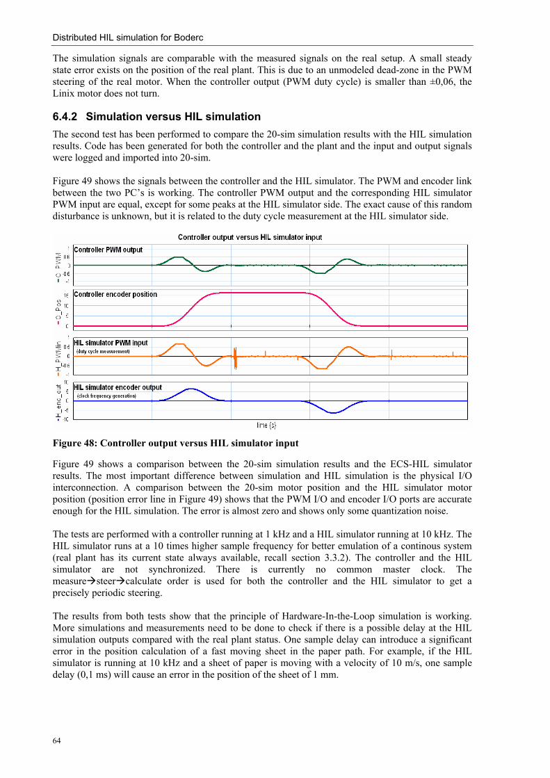
Distributed HIL simulation for Boderc
64
The simulation signals are comparable with the measured signals on the real setup. A small steady state error exists on the position of the real plant. This is due to an unmodeled dead-zone in the PWM steering of the real motor. When the controller output (PWM duty cycle) is smaller than ±0,06, the Linix motor does not turn.
6.4.2 Simulation versus HIL simulation The second test has been performed to compare the 20-sim simulation results with the HIL simulation results. Code has been generated for both the controller and the plant and the input and output signals were logged and imported into 20-sim. Figure 49 shows the signals between the controller and the HIL simulator. The PWM and encoder link between the two PC’s is working. The controller PWM output and the corresponding HIL simulator PWM input are equal, except for some peaks at the HIL simulator side. The exact cause of this random disturbance is unknown, but it is related to the duty cycle measurement at the HIL simulator side.
Figure 48: Controller output versus HIL simulator input
Figure 49 shows a comparison between the 20-sim simulation results and the ECS-HIL simulator results. The most important difference between simulation and HIL simulation is the physical I/O interconnection. A comparison between the 20-sim motor position and the HIL simulator motor position (position error line in Figure 49) shows that the PWM I/O and encoder I/O ports are accurate enough for the HIL simulation. The error is almost zero and shows only some quantization noise. The tests are performed with a controller running at 1 kHz and a HIL simulator running at 10 kHz. The HIL simulator runs at a 10 times higher sample frequency for better emulation of a continous system (real plant has its current state always available, recall section 3.3.2). The controller and the HIL simulator are not synchronized. There is currently no common master clock. The measure steer calculate order is used for both the controller and the HIL simulator to get a precisely periodic steering. The results from both tests show that the principle of Hardware-In-the-Loop simulation is working. More simulations and measurements need to be done to check if there is a possible delay at the HIL simulation outputs compared with the real plant status. One sample delay can introduce a significant error in the position calculation of a fast moving sheet in the paper path. For example, if the HIL simulator is running at 10 kHz and a sheet of paper is moving with a velocity of 10 m/s, one sample delay (0,1 ms) will cause an error in the position of the sheet of 1 mm.

Distributed HIL simulation for Boderc
65
Figure 49: 20-sim simulation versus HIL simulation


Distributed HIL simulation for Boderc
67
7 Conclusions & Recommendations
7.1 Conclusions
Boderc HIL simulation setup At the beginning of this project, there was no hardware available for a distributed HIL simulation setup. Currently, the distributed ECS part of the setup is ready to use (See Figure 50 for a picture). The HIL simulation part is not finished. The I/O boards are available, but a dedicated powerful HIL simulation PC has to be ordered. The HIL simulation part is on the moment implemented on one of the ECS PC/104’s. The foundation for experiments with HIL simulation and controller architectures is ready. The distributed ECS can be used together with 20-sim code generation to test control software. The code generation and compilation process is completely automated. Knowlegde about Linux, the underlying compilation process and the hardware access is not required to operate the setup. The chosen FPGA I/O board turned out to be a good choice for both the ECS and the HIL simulator. The flexibility of the FPGA configurations enables a broad range of applications, not limited to HIL simulation.
Figure 50: Boderc HIL simulation setup - ECS part with Linix
Distributed controller & CAN The current demonstration setup does not use a distributed controller. The main reason is that the CT CAN linkdrivers are not capable of running in a hard real-time environment. For the Linix setup, a distributed controller was not needed. The CAN bus is currently only in use for data logging. A distributed controller requires a modification in the 20-sim models and code generation to split up the controller into parts. Redistribution with CT is no problem, but the current code generation template generates one single Controller process.
HIL simulation The testresults in the previous chapter show that HIL simulation of the Linix setup is working. The results are good results for the interconnection of two Anything I/O boards. The generated software for both the controller and the HIL simulator behave exactly the same as within the 20-sim simulation in spite of the presence of real I/O hardware and the conversion to and from PWM and encoder signals. Accurate measurements about extra delay’s are currently not available. This needs further investigation. Not all required inputs/outputs for the Boderc paperpath simulation are available. The current setup has no dedicated digital sensor inputs, besides the general purpose I/O pins. An extension with digital inputs that can generate an interrupt is recommended

Distributed HIL simulation for Boderc
68
Communicating Threads The CT library turned out to be a simple way for multithreaded programming. The concept of channel communication has a great potential in a distributed environment, because redistribution of processes does not require changes inside the processes itself, but only in the channel links between them. The CT library is extended with many new linkdrivers for external channel communication. Communication linkdrivers for CAN & TCP/IP sockets and I/O linkdrivers for the parallel port and the various FPGA I/O configurations. The new remote linkdriver concept was ported from C to the C++ version and was used to provide support for multiple CT channels over one communication link. All linkdrivers are working, but not without problems. Due to problems with blocking CT programs when using Linux system calls and the lacking of userspace acces to interrupts, the CAN linkdriver required to make a workaround. Normal device driver access led to blocking system calls when no data was available, so interrupts were required for channel communication. The chosen workaround was to convert CAN interrupts in the Linux kernel to signals (software interrupts) for waking up a CT linkdriver. This resulted in a working CAN linkdriver, but it turned out that it was not useable in a hard-real-time RTAI environment. Using the linkdriver causes RTAI to return to a soft-real-time Linux environment. During the development of CT-based software, it was discovered that the Linux version has currently no timing support. All function calls related to time are not implemented yet. For controller software design, this became a problem. Besides the hard-real-time environment facilities, the timing function calls of RTAI/LXRT were used to get precise timing for control purposes.
7.2 Recommendations The ECS part of distributed HIL simulation setup is ready to use. The HIL simulation is also working, but a lot of effort is still needed to use the setup for the Boderc project. Especially the CT library can be improved at several points.
CT library • Add timing support to CT. Implement at least a good Thread::sleep and Thread::sleepUntil to
have some timing support under Linux. A better solution is to make use of the timing capabilities of RTAI/LXRT and the event system of Portable Threads (Engelschall, 2003) and to create a separate Timer object that handles all timing within CT.
• Rewrite the Idle thread to prevent busy waiting and burning CPU cycles. This saves power. • Make it possible to use OS threads instead of the own CT threads because of difficulties with
pthreads under linux. Another option is to look at the Portable Threads library implementation on how to prevent a blocking Linux function to block the whole CT program. Using a separate operating system thread will significantly decrease the performance of a context switch, but it will enable the CT user to use standard system calls and, if needed, PThreads. Especcially for applications where the performance is less important (e.g. the user interface) this will decrease the programming time, because one does not need to worry about possible blocking system calls.
• The current CT library relies on hardware interrupts as external events to wake-up suspended processes, reading from external channels. Access to hardware interrupts is under Linux only possible inside the kernel. Userspace CT programs have no access to hardware interrupts and linkdrivers that rely on interrupts do not work. RTAI/LXRT has the possibility to transfer interrupts from the kernel to userspace. The working of this approach should be investigated together with CT, to see if this is a solution for interrupt driven linkdrivers in userspace.
CAN • Rewrite the Peak System CAN driver to be compatible with RTAI. The current driver is not
RTAI compatible and cannot be used in a hard-real-time RTAI/LXRT environment • Using LXRT gives the possibility to use userspace interrupt handlers. It would be useful to
investigate this possibility in combination with the CAN linkdriver. Replace the signal solution with an userspace interrupt handler solution. Main advantage is that the CAN
Distributed HIL simulation for Boderc
69
linkdriver can then be used in a hard-real-time RTAI/LXRT environment (with the modified PCAN driver).
Anything I/O board • Create an extension (hardware and VHDL code) for the Anything I/O board that provides
access to the analog domain. This is not required for the Boderc project, but useful for other projects at the Control Laboratory (e.g. for the snake board).
• Create an extension print for the Anything I/O board with some I/O buffers for testing purposes. The FPGA I/O board has no external buffering. An accidental short circuit or interchange of input and output may end in FPGA damage.
• Extend the current ECS/HIL simulation FPGA configuration with digital sensor inputs that can generate interrupts.
20-sim models & code generation • Create a 20-sim model framework with one submodel per ECS PC and HIL simulator to
facilitate (submodel) code generation for a distributed controller. The submodels can be filled later with a part of the distributed controller that should run on a specific PC.
• More simulations and measurements need to be done to check if there is a possible delay at the HIL simulation outputs compared with the real plant status. One sample delay can introduce a significant error in the position calculation of a fast moving sheet in the paper path. For example, if the HIL simulator is running at 10 kHz and a sheet of paper is moving with a velocity of 10 m/s, one sample delay (0,1 ms) will cause an error in the position of the sheet of 1 mm.
• Replace the ADSP dll calls (and its submodels) in the used 20-sim models with general purpose dll calls. The current Boderc templates still use the ADSP dll and ADSP related function calls to be compatible with the Linix models used on the ADSP board.

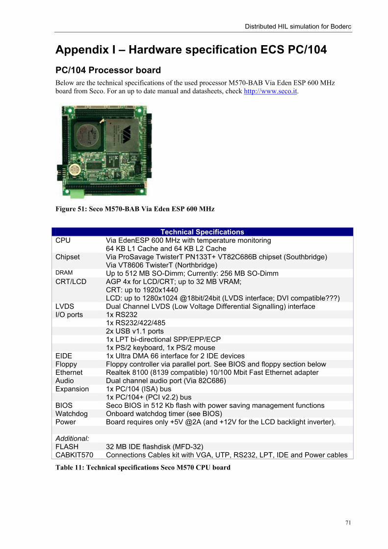
Distributed HIL simulation for Boderc
71
Appendix I – Hardware specification ECS PC/104 PC/104 Processor board Below are the technical specifications of the used processor M570-BAB Via Eden ESP 600 MHz board from Seco. For an up to date manual and datasheets, check http://www.seco.it.
Figure 51: Seco M570-BAB Via Eden ESP 600 MHz
Technical Specifications
CPU Via EdenESP 600 MHz with temperature monitoring 64 KB L1 Cache and 64 KB L2 Cache
Chipset Via ProSavage TwisterT PN133T+ VT82C686B chipset (Southbridge) Via VT8606 TwisterT (Northbridge)
DRAM Up to 512 MB SO-Dimm; Currently: 256 MB SO-Dimm CRT/LCD AGP 4x for LCD/CRT; up to 32 MB VRAM;
CRT: up to 1920x1440 LCD: up to 1280x1024 @18bit/24bit (LVDS interface; DVI compatible???)
LVDS Dual Channel LVDS (Low Voltage Differential Signalling) interface I/O ports 1x RS232 1x RS232/422/485 2x USB v1.1 ports 1x LPT bi-directional SPP/EPP/ECP 1x PS/2 keyboard, 1x PS/2 mouse EIDE 1x Ultra DMA 66 interface for 2 IDE devices Floppy Floppy controller via parallel port. See BIOS and floppy section below Ethernet Realtek 8100 (8139 compatible) 10/100 Mbit Fast Ethernet adapter Audio Dual channel audio port (Via 82C686) Expansion 1x PC/104 (ISA) bus 1x PC/104+ (PCI v2.2) bus BIOS Seco BIOS in 512 Kb flash with power saving management functions Watchdog Onboard watchdog timer (see BIOS) Power Board requires only +5V @2A (and +12V for the LCD backlight inverter). Additional: FLASH 32 MB IDE flashdisk (MFD-32) CABKIT570 Connections Cables kit with VGA, UTP, RS232, LPT, IDE and Power cables
Table 11: Technical specifications Seco M570 CPU board
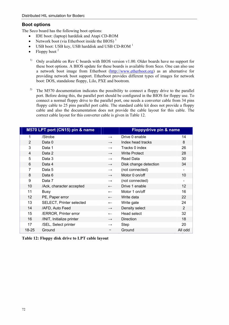
Distributed HIL simulation for Boderc
72
Boot options The Seco board has the following boot options:
• IDE boot: (laptop) harddisk and Atapi CD-ROM • Network boot (via Etherboot inside the BIOS) 1 • USB boot: USB key, USB harddisk and USB CD-ROM 1 • Floppy boot 2
1) Only available on Rev C boards with BIOS version v1.00. Older boards have no support for
these boot options. A BIOS update for these boards is available from Seco. One can also use a network boot image from Etherboot (http://www.etherboot.org) as an alternative for providing network boot support. Etherboot provides different types of images for network boot: DOS, standalone floppy, Lilo, PXE and bootrom.
2) The M570 documentation indicates the possibility to connect a floppy drive to the parallel port. Before doing this, the parallel port should be configured in the BIOS for floppy use. To connect a normal floppy drive to the parallel port, one needs a converter cable from 34 pins floppy cable to 25 pins parallel port cable. The standard cable kit does not provide a floppy cable and also the documentation does not provide the cable layout for this cable. The correct cable layout for this converter cable is given in Table 12.
M570 LPT port (CN15) pin & name Floppydrive pin & name 1 /Strobe → Drive 0 enable 14 2 Data 0 → Index head tracks 8 3 Data 1 → Tracks 0 index 26 4 Data 2 → Write Protect 28 5 Data 3 → Read Data 30 6 Data 4 → Disk change detection 34 7 Data 5 → (not connected) - 8 Data 6 → Motor 0 on/off 10 9 Data 7 → (not connected) - 10 /Ack, character accepted ← Drive 1 enable 12 11 Busy ← Motor 1 on/off 16 12 PE, Paper error ← Write data 22 13 SELECT, Printer selected ← Write gate 24 14 /AFD, Auto Feed → Density select 2 15 /ERROR, Printer error ← Head select 32 16 /INIT, Initialize printer → Direction 18 17 /SEL, Select printer → Step 20
18-25 Ground − Ground All odd i
Table 12: Floppy disk drive to LPT cable layout

Distributed HIL simulation for Boderc
73
Peak Systems PC/104 CAN board
Settings The PC/104 CAN boards in the HIL setup are configured to use IRQ 5 and I/O address 0x300 for CAN communication.
Technical information
Figure 52: PCAN PC/104 board, CAN connector layout
Technical data Baudrate Up to 1 MBaud CAN controller 1 Philips SJA 1000 CAN controller with 16 MHz clock frequency CAN specification 2.0a (standard frame) and 2.0b (extended frame) Bus PC/104 compliant (no PC/104+ stack through connector Connector 9-pole SUB-D according to CiA-recommendation DS 102-1 Galvanic isolation Up to 1000 Volt Line drivers Philips 82C251 Software PCANVIEW 2.0L for Win 9x/ME and Win NT/2000/XP CANView for DOS Device driver (sys,VxD) and interface-DLL for Win 9x/ME and Win
NT/2000/XP Example program with source-code for VB, BB5 and VC on disk Linux drivers available at the website (http://www.peak-system.com/) Parallel use of multiple card in one PC/104 system (interrupt sharing) 14 different I/O- addresses (200h –3A0h) and 8 different IRQ-maps (3, 4, 5, 7, 10, 11, 12 and 15) selectable Hardware reset from software possible
Table 13: Technical data PCAN PC/104


Distributed HIL simulation for Boderc
75
Appendix II - Getting started PC/104+ CPU board Introduction This appendix describes in short how to boot the Seco PC/104+ pc for the first time.
Requirements • Seco M570 CPU board & IDE flashdisk • Seco M570 manual • Seco M570 Cable kit • Powersupply (5V, 2,5 A) • Standard 3,5” Floppy drive • Parallel port -to- floppy converter cable • Bootdiskette with DOS, Linux or Etherboot network boot image (for local boot) • For network boot: a working network bootserver (e.g. A Linux DHCP server and TFTPboot
server)
Preparations • Connect the IDE flashdisk • Connect the following cables to the PC/104 board: LPT, VGA, keyboard/mouse • Connect the green power connector to a 5V power supply (e.g. a normal PC powersupply).
See the M570 manual for the connection scheme • Turn on the PC/104 and enter the BIOS by pressing DEL for the floppy drive settings • Basic CMOS: Floppy drive A: 1,44 Mb
(You should see the flash disk here as Hard disk C:) • Advanced CMOS: First boot device -> Floppy • Chipset configuration: Parallel connected to -> FDC • Save the settings to the CMOS and turn off the PC • Connect the floppy drive to the parallel port using the converter cable (for local boot)
First time boot Option 1: Boot DOS/Linux from floppy Just insert a bootable DOS/Linux floppy and copy the operating system to the flash disk, just like one would do on a normal PC. The flashdisks are preformatted with the FAT filesystem. Option 2: Boot DOS/Linux from the network • To boot the PC directly from the network, you need a at least a BIOS revision 1.00 or a diskette
with a bootimage. The old Seco BIOS (v0.03) is not able to boot directly from the network. An Etherboot floppy bootimage for the onboard networkcard can be obtained from http://rom-o-matic.net. You need a “Floppy Bootable ROM image (.zdsk) for the RTL 8139 networkcard. Follow the instructions on the website to put the image on a floppy disk. If your pc has a v1.00 BIOS (or higher), enable the “Enhanced BIOS loading” option inside the BIOS. This will enable the Etherboot support inside the BIOS.
See appendix V for the installation of a remote boot server.

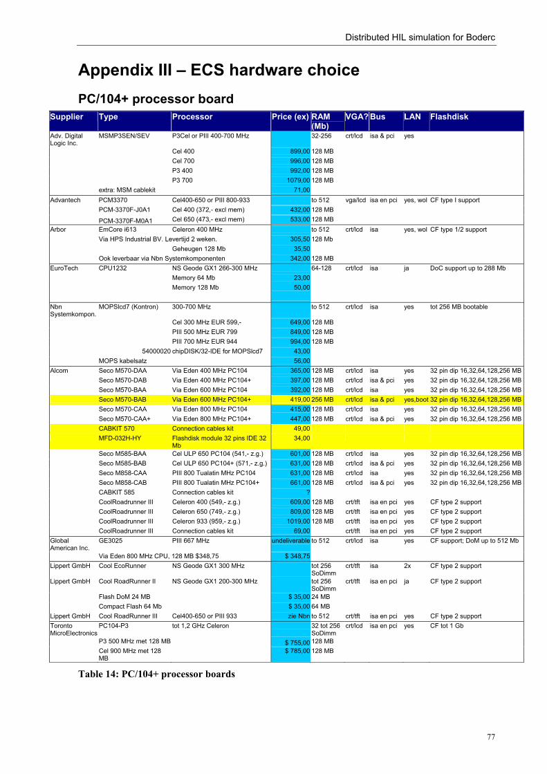
Distributed HIL simulation for Boderc
77
Appendix III – ECS hardware choice PC/104+ processor board
Table 14: PC/104+ processor boards
Supplier Type Processor Price (ex) RAM (Mb)
VGA? Bus LAN Flashdisk
Adv. Digital Logic Inc.
MSMP3SEN/SEV P3Cel or PIII 400-700 MHz 32-256 crt/lcd isa & pci yes
Cel 400 899,00 128 MB Cel 700 996,00 128 MB P3 400 992,00 128 MB P3 700 1079,00 128 MB extra: MSM cablekit 71,00 Advantech PCM3370 Cel400-650 or PIII 800-933 to 512 vga/lcd isa en pci yes, wol CF type I support PCM-3370F-J0A1 Cel 400 (372,- excl mem) 432,00 128 MB PCM-3370F-M0A1 Cel 650 (473,- excl mem) 533,00 128 MB Arbor EmCore i613 Celeron 400 MHz to 512 crt/lcd isa yes, wol CF type 1/2 support Via HPS Industrial BV. Levertijd 2 weken. 305,50 128 Mb Geheugen 128 Mb 35,50 Ook leverbaar via Nbn Systemkomponenten 342,00 128 MB EuroTech CPU1232 NS Geode GX1 266-300 MHz 64-128 crt/lcd isa ja DoC support up to 288 Mb Memory 64 Mb 23,00 Memory 128 Mb 50,00 Nbn Systemkompon.
MOPSlcd7 (Kontron) 300-700 MHz to 512 crt/lcd isa yes tot 256 MB bootable
Cel 300 MHz EUR 599,- 649,00 128 MB PIII 500 MHz EUR 799 849,00 128 MB PIII 700 MHz EUR 944 994,00 128 MB 54000020 chipDISK/32-IDE for MOPSlcd7 43,00 MOPS kabelsatz 56,00 Alcom Seco M570-DAA Via Eden 400 MHz PC104 365,00 128 MB crt/lcd isa yes 32 pin dip 16,32,64,128,256 MB Seco M570-DAB Via Eden 400 MHz PC104+ 397,00 128 MB crt/lcd isa & pci yes 32 pin dip 16,32,64,128,256 MB Seco M570-BAA Via Eden 600 MHz PC104 392,00 128 MB crt/lcd isa yes 32 pin dip 16,32,64,128,256 MB Seco M570-BAB Via Eden 600 MHz PC104+ 419,00 256 MB crt/lcd isa & pci yes,boot 32 pin dip 16,32,64,128,256 MB Seco M570-CAA Via Eden 800 MHz PC104 415,00 128 MB crt/lcd isa yes 32 pin dip 16,32,64,128,256 MB Seco M570-CAA+ Via Eden 800 MHz PC104+ 447,00 128 MB crt/lcd isa & pci yes 32 pin dip 16,32,64,128,256 MB CABKIT 570 Connection cables kit 49,00 MFD-032H-HY Flashdisk module 32 pins IDE 32
Mb 34,00
Seco M585-BAA Cel ULP 650 PC104 (541,- z.g.) 601,00 128 MB crt/lcd isa yes 32 pin dip 16,32,64,128,256 MB Seco M585-BAB Cel ULP 650 PC104+ (571,- z.g.) 631,00 128 MB crt/lcd isa & pci yes 32 pin dip 16,32,64,128,256 MB Seco M858-CAA PIII 800 Tualatin MHz PC104 631,00 128 MB crt/lcd isa yes 32 pin dip 16,32,64,128,256 MB Seco M858-CAB PIII 800 Tualatin MHz PC104+ 661,00 128 MB crt/lcd isa & pci yes 32 pin dip 16,32,64,128,256 MB CABKIT 585 Connection cables kit ? CoolRoadrunner III Celeron 400 (549,- z.g.) 609,00 128 MB crt/tft isa en pci yes CF type 2 support CoolRoadrunner III Celeron 650 (749,- z.g.) 809,00 128 MB crt/tft isa en pci yes CF type 2 support CoolRoadrunner III Celeron 933 (959,- z.g.) 1019,00 128 MB crt/tft isa en pci yes CF type 2 support CoolRoadrunner III Connection cables kit 69,00 crt/tft isa en pci yes CF type 2 support Global American Inc.
GE3025 PIII 667 MHz undeliverable to 512 crt/lcd isa yes CF support; DoM up to 512 Mb
Via Eden 800 MHz CPU, 128 MB $348,75 $ 348,75 Lippert GmbH Cool EcoRunner NS Geode GX1 300 MHz tot 256
SoDimm crt/tft isa 2x CF type 2 support
Lippert GmbH Cool RoadRunner II NS Geode GX1 200-300 MHz tot 256 SoDimm
crt/tft isa en pci ja CF type 2 support
Flash DoM 24 MB $ 35,00 24 MB Compact Flash 64 Mb $ 35,00 64 MB Lippert GmbH Cool RoadRunner III Cel400-650 or PIII 933 zie Nbn to 512 crt/tft isa en pci yes CF type 2 support
PC104-P3 tot 1,2 GHz Celeron 32 tot 256 SoDimm
crt/lcd isa en pci yes CF tot 1 Gb Toronto MicroElectronics
P3 500 MHz met 128 MB $ 755,00 128 MB Cel 900 MHz met 128
MB $ 785,00 128 MB

Distributed HIL simulation for Boderc
78
PC/104 CAN board Supplier Typenummer Bus Price #CAN Std Controller Fifo Galv Max.
bitrateOverzicht CAN bordjes - PC104 Advanced Digital Logic Inc.
MSMCAN PC104 136,00 1 2.0A/B i82C527 no 500 kBaud -
via LVP Industrial Aton Systems CAN-PC104 PC104 109,00 1 2.0A/B SJA1000 no 1 Mbit/s CAN-PC104 opto PC104 150,00 2 2.0A/B SJA1000 yes 1 Mbit/s CD Systems 645802 CAN PC104 PC104 228,00 2 2.0A/B SJA1000;
Intel 82527; Siemens 81C91 of all three
yes 1 Mbit/s
CD Systems 6459-02 CAN PC104/331 PC104 350,00 1 SJA1000 yes 1 Mbit/s CD Systems Manual+drivers (compulsory) 62,00 ESD GmbH CAN-PC104/331 PC104 350,00 1 2.0A/B SJA1000 512 bytes yes 1 Mbit/s ESD GmbH CAN-PC104/200-P PC104 200,00 1 2.0A/B SJA1000 - yes 1 Mbit/s for all: driver licence 60,00 Compusory:a driver which is an object license windows&linux. Emtrion Gmbh Hico.CAN-104-2 PC104 370,00 2 2.0A/B SJA1000 yes 2x
1Mbit/s (was: Hitex) Hico.CAN-104-2H PC104 420,00 2 daarnaast voor een van de 3 types eenmalig een
software pakket a EUR 420 nodig (zie mail) I+Me Actia Informatik InduCAN 104 Pc104 260,00 1 2.0A/B SJA1000 64 bytes yes 1 Mbit/s NBN System komponenten
Seco M441 Pc104 137,00 1 2.0A/B Intel 82527 15x8 yes 1 Mbit/s
Peak System Technik PCAN Dongle Parallel->Can
145,00 1 2.0A/B SJA1000 yes 1 Mbit/s
Peak System Technik PCAN PC104 PC104 128,00 1 2.0A/B SJA1000 no 1 Mbit/s Peak System Technik PCAN PC104 opto PC104 169,00 1 2.0A/B SJA1000 yes 1 Mbit/s Peak System Technik various types of CAN cables and T-splitters
available
Realtime Devices USA ECAN1000HR PC104 $ 175,00
1 2.0B SJA1000 64 bytes yes 1 Mbit/s
Overzicht CAN bordjes - PCI ESD GmbH CAN-PCI/331-1 PCI 500,00 1 2.0A/B SJA1000 512 bytes yes 1 Mbit/s ESD GmbH CAN-PCI/331-2 PCI 655,00 2 2.0A/B SJA1000 512 bytes yes 1 Mbit/s ESD GmbH CAN-PCI/200-1 PCI 254,00 1 2.0A/B SJA1000 yes 1 Mbit/s ESD GmbH CAN-PCI/200-2 PCI 325,00 2 2.0A/B SJA1000 yes 1 Mbit/s Emtrion Gmbh Hico.CAN-PCI-2 PCI 420,00 2 2.0A/B SJA1000 2x
1Mbit/s via Si-Kwadraat PCI IntelliCAN PCI 545,00 2.0A/B SJA1000 yes 1 Mbit/s Peak System Technik PCAN PCI PCI 200,00 1 2.0A/B SJA1000 no 1 Mbit/s Peak System Technik PCAN PCI opto PCI 270,00 1 2.0A/B SJA1000 yes 1 Mbit/s
Table 15: Overview available CAN boards
Supplier Type Price
LVP Industrial Tri-M HE104-512 High efficiency Pc/104 powersupply +5V/10A, +12V/2A
252,00
JMM 512 50W +5V/+12V 250,00 JMM 512 50W +5V/+12V/-5V/-12V 303,00 NBN System komponenten
JMM 512 50W +5V/+12V 198,00
JMM 512 50W +5V/+12V/-5V/-12V 247,00 Target MicroATX 200W 20,00 For comparison: a typical 300 W ATX power supply 25,00
Table 16: Overview PC/104 power supplies

Distributed HIL simulation for Boderc
79
Appendix IV – Software installation ECS PC/104 Introduction This appendix describes how to build an embedded Linux installation with RTAI real-time support from scratch. The DOS installation on the ECS PC’s will also be discussed. Usernames and passwords for the ECS PC’s can be found at the end of this appendix.
Linux installation
Linux basics The Linux operating system consists of two parts, the Linux kernel and a root file system with shared libraries, utilities and programs. The kernel is the core of the Linux project and provides services like memory management, resource management, hardware access, etcetera to other operating system components and user programs. The Unix style root file system contains all necessary configuration settings, libraries, system tools and programs. This file system can usually be found on the hard disk. Sometimes, this file system is put on the network or on a ram disk for instance on diskless pc’s. During the boot-up, the Linux kernel will be loaded into memory (from disk or network) and then executed. After setting up some basic system properties required to locate and open the root file system, the kernel will start its first process called init (found on the root file system). From the init process, the system can start multiple programs for networking, user interaction, and etcetera.
Kernel Download the Linux kernel from http://www.kernel.org (e.g. linux-2.4.26.tar.bz2) and extract this zip file using bunzip2 and tar. To use the RTAI Real-time Extensions, download the latest RTAI version from http://www.rtai.org (e.g. rtai-3.1-test2.tar.bz2) and extract this BZip file. The required kernel patch can be found in the directory /rtai-core/arch/i386/patches/. Copy the patch corresponding with the kernel version to the kernel source directory. Go to the kernel source directory and apply this patch to the extracted source using: patch -p1 <hal13c2-2.4.26.patch Now, configure the kernel on the normal way, using make menuconfig The used kernel configuration can be found in the ecs/kernel/.config file. Copy this file to the directory containing the kernel source and run make menuconfig to verify the settings. Important configuration options:
• Pentium-MMX processor family • General setup Adeos support (CONFIG_ADEOS) • PCI and ISA support • No Power Management or ACPI support (because of RTAI) • Set version information on all module symbols => disabled • Parallel port support (for the Peak System CAN driver) • Loopback device support • Ram disk support (16386 kb) • Floppy drive support (if needed) • Via 82CXX chipset support • Realtek 8139 PCI Fast Ethernet adapter support • DOS FAT fs support (MSDOS & VFAT) • Second Extended filesystem support (EXT2) • NFS v3 (Network File System)

Distributed HIL simulation for Boderc
80
For remote boot additional: • TCP/IP networking – IP: kernel level auto configuration (DHCP & BOOTP) • Network File System – Root file system on NFS
The Via Eden CPU has a TSC, but the CPU is not listed in the kernel configuration menu’s, therefore support for this option needs to be added by hand. Add after finishing the menu based configuration, the option CONFIG_X86TSC=y to the .config file. This will result in a more accurate timing under RTAI. Compile the kernel with: make dep make bzImage make modules make modules_install INSTALL_MOD_PATH={ROOT_FS}/ where {ROOT_FS} is the directory in which the new filesystem should be created. E.g. /home/marcel/ecs/linux/fs After compilation, the kernel image can be found at the location: {kernel_source_dir}/arch/i386/boot/bzImage
Root file system
Introduction The Linux root file system will be put on a ram disk. In this way, it is possible to use more than 32 Mb for the root file system, by placing a compressed version on disk or on a network drive. An additional advantage of the ram disk is the speed. Running programs from a ram disk is much faster than from a flash disk. There is also a disadvantage. When the power is turned off, all changes on the ram disk are lost. This can be solved by putting some parts on the flash disk or network drive and not on the ram disk. A script was written for automatic creation of a compressed root file system image (similar to a Norton Ghost disk image). See the end of this section. Below, the process of creating the root files system by hand will be described.
Directory structure First, the basic directory layout has to be created. According to the 'File Hierarchy Standard' the Linux root file system should contain the following directories: bin, etc, dev, home, lib, proc, root sbin, usr, var. mkdir bin etc dev home lib proc root sbin usr var
Software configuration and installation Software, libraries and script have to be added to the filesystem to create a useful Linux system. The table below contains an overview of the required software.

Distributed HIL simulation for Boderc
81
Package Version Description uClibc 0.9.26 C libraries for embedded Linux systems (alternative for glibc)
BusyBox 1.00 Multi-call binary that provides many common Linux tools
Tinylogin 1.4 Multi-call binary for login- and user management
OpenSSH Secure remote shell, remote copy and remote execute
Peak CAN drivers 1.40 (CT) Kernel module and shared library for the Peak System CAN board
RTAI & LXRT 3.1 Real-time extension for the Linux kernel and userspace
I/O drivers 1.00 Kernel module and shared library for the Anything I/O board
table 17: Required packages
uClibc library One of the required shared libraries is the GNU C library, Glibc. Almost all Linux programs are written in C/C++. These programs use a shared library called libc/glibc which contains the basic C and C++ functions. Because this library is quite voluminous and the disk space is limited, a replacement library, uClibc will be used. This Glibc like library is especially aimed at small Linux systems and embedded devices. The uClibc library tries to maintain the same functionality as the Glibc library but is considerably smaller. If all required programs and tools are compiled using this library, the required disk space can be reduced considerably. The uClibc source can be downloaded from http://www.uclibc.org/downloads/. For the purpose of creating a root file system, only the uClibc libraries and a cross platform compiler are required. For this purpose, uClibc provides a toolchain with the uClibc libraries and a gcc cross compiler. To download the sources for this toolchain, visit http://uclibc.org/cgi-bin/cvsweb/toolchain/ and download the tarball file. After extraction of this file, run make (as user, not as root for safety) This script will automatically download and compile the required components. This may take a couple of hours to complete (depending on the download speed and processing power). Remark 1:
For the creation of a complete root file system with all required tools and a gcc compiler that uses uClibc instead of Glibc, one can download the buildroot kit instead of the toolchain: Fetch the latest tarball from http://uclibc.org/cgi-bin/cvsweb/buildroot/ Just untar and run make (for safety: run as user, not as root). This script will create automatically a complete linux root filesystem with all required tools for compiling programs against uClibc. Because all required tools and programs are downloaded and compiled on demand, the execution of this script may take up to one day (depending on the speed of the Internet connection and the processing power). My experience with this script is that it delivers most of the time a not working toolchain and a file system with missing programs. The script downloads normally the daily development snapshots of Busybox and uClibc. This may result in a version that will not compile. Besides this, the generated root filesystem is around 70 Mb and can therefore only be used to copy programs/libraries, for a network boot system or for testing purposes using User Mode Linux (UML; run Linux under Linux).
Remark 2: At the moment of writing this documentation, there were announcements of a new Debian based distribution targeted at embedded and small systems (uWoody). They plan to port Debian Woody to uClibc. Installation of an uClibc will become much easier when this distribution is available. Check the http://www.emdebian.org/ and http://www.uclibc.org for the current status. (A first beta version of uWoody is already available).
After compilation, copy the toolchain_i386 directory to /usr/i386-linux-uclibc/.
Distributed HIL simulation for Boderc
82
To compile programs with this cross compiler, one can modify the path by adding the uClibc directories in front of the path environment variable. $ export PATH=/usr/i386-linux-uclibc/:$PATH Check with: $ gcc –v if the default compiler is now the gcc cross compiler.
Busybox Busybox combines tiny versions of many common UNIX utilities into a single small multicall executable. Dependent on the name of the symlink to the Busybox binary, it will behave like the normal Linux utility with that name. Busybox provides replacements for most of the utilities you usually find in GNU fileutils, shellutils, etc. The utilities in BusyBox generally have fewer options than their full-featured GNU cousins; however, the options that are included provide the expected functionality and behave very much like their GNU counterparts. BusyBox provides a fairly complete environment for any small or embedded system. BusyBox has been written with size-optimization and limited resources in mind. It is also extremely modular so one can easily include or exclude commands (or features) at compile time. For the embedded target, the following programs are required, sorted by destination directory: /bin
ash, cat,chgrp,chmod,chown,cp,date,dd,df,dmesg,false, fgrep, grep, gunzip, gzip, hostname, kill, ln, ls, mkdir, mknod, mktemp, more, mount, mv, netstat, ping, pipe_progress, ps, pwd, rm, rmdir, run-parts, sh, sleep, stty, sync, tar, touch, true, umount, uname, uncompress, usleep, vi, zcat
/sbin halt, ifconfig, ifdown, ifup, init, insmod, klogd, losetup, lsmod, makedevs, modprobe, poweroff, reboot, rmmod, route, start-stop-daemon, swapoff, swapon, syslogd, udhcpc
/usr/bin basename, bunzip2, bzcat, clear, cut, dirname, dos2unix, dpkg, dpkg-deb, du, env, find, free, ftpget, ftpput, id, killall, logger, mesg, nslookup, printf, readlink, reset, sort, tail, test, top, tty, uniq, unix2dos, unzip, uptime, wget, which, whoami, yes
/usr/sbin chroot, udhcpd
To generate a Busybox executable with the above programs, copy the existing .config file to the Busybox directory and run make menuconfig to check and/or modify the configuration. Then compile Busybox using the uClibc gcc compiler with: make CC=/usr/i386-linux-uclibc/usr/bin/gcc The CC= option passes on the alternave gcc compiler to the compile script. To install Busybox and the required links into the root filesystem, run: make PREFIX=$ROOT_FS install where $ROOT_FS is the directory in which the rootfs should be created. Now, the Busybox binary and the corresponding symlinks are installed.
Tinylogin TinyLogin is a suite of tiny Linux utilities for handling logging into, being authenticated by, changing one's password for, and otherwise maintaining users and groups on an embedded system. It also provides shadow password support to enhance system security. Tinylogin is based on the same principle as Busybox. It provides a single small multicall replacement binary for common Linux tools.

Distributed HIL simulation for Boderc
83
The required programs for our application are (sorted by destination directory): /bin
addgroup, adduser, delgroup, deluser, login, su /sbin
getty, sulogin /usr/bin
passwd The compilation and installation process for Tinylogin is comparable with Busybox. First, copy the existing .config file to the tinylogin directory and run make menuconfig to check and/or modify the configuration options. Then compile Tinylogin using the uClibc gcc compiler with: make CC=/usr/i386-linux-uclibc/usr/bin/gcc To install Busybox and the required links into the root filesystem, run: make PREFIX=$ROOT_FS install The Tinylogin binary and the corresponding symlinks are installed.
OpenSSH To make remote administration of the embedded targets possible, the OpenSSH suite will be used. OpenSSH is a secure version for telnet like programs for remote login purposes. The Open SSH suite contains, among others, the following useful tools:
• ssh: remote login • sshd: remote login server • • scp: for secure copying of files from pc to pc • rsh: run programs on another computer without logging first
Open SSH can be found at: http://www.openssh.com/. According to the installation instructions, the openssl library and zlib library are also required. http://www.gzip.org/zlib/ http://www.openssl.org/
Peak CAN devicedrivers To install the Peak System PCAN driver for Linux, download a recent version of the driver from http://www.peak-system.com/linux/index.htm. Extract the files from the archive and look at the installation instructions for manual installation. These can be found in the installation manual in the documentation directory. The installation process for the embedded target is almost the same, with one difference. It is not possible to compile the kernel module, the driver and the testprograms at once because to different compilers have to be used. Use the makefiles in the subdirectories and not the makefiles in the rootdirectory. Point of attention: • To use the Peak System kernel module, the kernel must have parallel port support (parport.o) • Do not compile the kernel module with the uClibc gcc compiler. Use the normal gcc compiler, also
used for the kernel compilation. • The library and the test programs have to be compiled with the uClibc gcc compiler using the extra
make option CC=/usr/i386-linux-uclibc/usr/bin/gcc To compile and install the Peak System driver execute (with root privileges) cd driver make mkdir $ROOT_FS/lib/modules/2.4.26-adeos/kernel/drivers/can
Distributed HIL simulation for Boderc
84
cp pcan.o $ROOT_FS/lib/modules/2.4.26-adeos/kernel/drivers/can/ cd ../lib make CC=/usr/i386-linux-uclibc/usr/bin/gcc cp libpcan.so.0.0 $ROOT_FS/usr/lib/ ln -sf $ROOT_FS/usr/lib/libpcan.so.0.0 $ROOT_FS/usr/lib/libpcan.so.0 ln -sf $ROOT_FS/usr/lib/libpcan.so.0.0 $ROOT_FS/usr/lib/libpcan.so cd ../test make
where $ROOT_FS is the path to the root file system to be created. Currently, the transmit testprogram provided with the drivers, does not compile using the uClibc compiler or a gcc v3.3 compiler because of altered functions between gcc 2.95 and gcc 3.3.
Anything I/O devicedrivers The installation procedure for the Anything I/O devicedrivers is similar to the PCAN driver. For more information about the installation of the Anything I/O devicedrivers, see appendix VII.
RTAI modules Use the extracted source files (already downloaded for the kernel patch) and copy the already made .config file to this directory. Detailed installation instructions can be found in the README.INSTALL file. In short, RTAI can be configured, compiled and installed using: make menuconfig make make install INSTALL_MOD_PATH=$ROOT_FS/ make dev INSTALL_MOD_PATH=$ROOT_FS/ PS. Because the RTAI modules are kernel modules, use the normal gcc compiler and not uClibc gcc.
Reducing disk space: strip & UPX To save diskspace, the Linux strip utility can be used. Before using this utility, make a backup of the original unstipped files for the case that the stripped versions are broken, because strip overwrites the binaries. It is not recommended to use strip on shared libraries. strip binary –-strip-debug This call removes all debugging symbols from libraries or executables. Another option for space saving is the Ultimate Packer for eXecutables (UPX). This is a cross platform executable compressor that reduces the size of Linux, DOS and Windows executables. The extra time for decompression (around 40 Mb/s) at the startup is almost neglegible. Using this utility in combination with a compressed root file system gives not much space winning, because of the double compression. http://upx.sourceforge.net/
Automatic creation of the compressed root filesystem image A small script was created for easy re-creation of the root filesystem, used on the embedded targets. This script creates the compressed root file system using an uncompressed copy of the already generated filesystem. This script can also be used to create your own root file system as long as you use the same directory layout as described below. The script can be found in the ecs/linux directory on the development machine (and in the HIL CVS repository, module: OS). This directory contains the following files and directories:

Distributed HIL simulation for Boderc
85
drwxr-xr-x 5 marcel marcel 120 Jan 7 12:33 ecs_pc1 drwxr-xr-x 5 marcel marcel 120 Jan 7 12:39 ecs_pc2 drwxr-xr-x 5 marcel marcel 120 Jan 7 12:39 ecs_pc3 drwxr-xr-x 5 marcel marcel 120 Jan 7 12:39 ecs_pc4 drwxr-xr-x 5 marcel marcel 120 Jan 7 12:40 ecs_pc5 drwxr-xr-x 17 root root 480 Jan 14 12:52 fs drwxr-xr-x 4 marcel marcel 136 Jan 12 09:57 kernel -rwxrwxrwx 1 marcel marcel 2788 Jan 14 15:57 mkrootfs drwxr-xr-x 7 root root 168 Jan 14 15:59 rootfs
The mkrootfs script creates a file named rootfs.gz inside the directory rootfs/x/ (with x=1..5) that contains the whole root filesystem for pc number x. This script can only be executed with root rights. The directory fs/ contains the uncompressed files shared for all 5 targets. The target specific files (e.g. hostname, ssh keys) can be found in the ecs_pcX/ folders. The mkrootfs script uses the /dev/loop0 device to create a Linux filesystem in a single file (Loopback filesystem). After copying all required files to this empty filesystem, this file will be compressed with gzip. The result is a compressed root file system image that can be loaded into a ramdisk by the Linux kernel.
Changing the compressed root filesystem image To change an existing root filesystem image, the image needs to be uncompressed and mouted as loopback device. See the listing below for the required commands: # gunzip rootfs.gz # ls rootfs # mkdir rootfsmount # losetup /dev/loop0 rootfs # mount –o loop /dev/loop0 rootfsmount # cd rootfsmount # ls bin data dev etc flash home lib linuxrc mnt opt proc root sbin tmp usr var The root filesystem is now mounted in the rootfsmount directory. To unmount the filesystem and to recreate the compressed filesystem image, run the following commands: # umount rootfsmount # rmdir rootfsmount # losetup –d /dev/loop0 # gzip rootfs # ls rootfs.gz For more information about these Linux tools and on how to use the loopback device, see the man pages of these tools.
DOS installation Besides the Linux installation, the ECS PC's contain also a small DOS installation. This DOS installation is small and not complete. It contains only the necessary utilities and drivers for running CT-programs and for CAN tests. In addition to the required tools, this DOS installation has networking support and USB mass storage support. Additional programs can therefore be provided on a networkdrive or on a USB harddisk/key.
Networking To enable the network under DOS, run the following program: C:\>startnet

Distributed HIL simulation for Boderc
86
This batchfile will load the required networkdrivers and maps the driveletter N: to the share \\ce177\ecsshare which exists on the development pc (under Linux: /data/ecs). For the login data, see the “Login Data” section at the end of this appendix.
USB harddisk/key To use an USB harddisk or USB key, run the program: C:\>usb.bat Remark:
Since BIOS revision 1.00, the Seco BIOS contains build-in support for USB harddisks and USB keys. It is under DOS not necessary anymore to load this driver first, due to the BIOS USB support. Enabling this ‘legacy’ USB support can however influence the real-time behaviour of RTAI, so enable this option only, when needed.
Executable compression To save valuable flashdisk space, the DOS executables can be compressed using the UPX utility (see the Linux section above for more information)
Bootmanager installation A bootmanager is required to choose between booting Linux, DOS or networkboot. To install the GRUB boot manager, see the “Bootmanager” section in appendix V.
Login data Below are the required username/password combinations for the ECS pc's: Linux: root distribhil$ ecs ecs#login DOS (network): ecs ecslogin

Distributed HIL simulation for Boderc
87
Appendix V - Remote boot server for the PC104 pc’s Introduction This appendix describes in short how to boot a Seco PC104+ pc from the network using a Linux pc as Remote Boot Server. After a short overview of the requirements and the backgrounds behind network booting, the installation procedure for remote boot from Linux wil be described step by step.
Requirements • Seco M570 CPU board with IDE flashdisk and a network connection • MAC address of the Seco board(s) • Linux pc with two networkcards (preferably) • GRUB bootloader on the flashdisk or if your pc has a v1.00 BIOS (or higher), enable the
“Enhanced BIOS loading” option inside the BIOS. This will enable the Etherboot support inside the BIOS.
For the rest of this appendix, it is assumed that a working DOS installation and/or Linux installation (with network support) are already available on the flashdisk.
Network boot overview Most systems that are network boot capable, have a bootrom on the networkcard or a “network boot” option inside the BIOS. This contains the first part of the bootstrap code. It does nothing more than enabling the network card and request boot information on the network. One could wonder how a station may boot over an IP network if it does not even know its own IP address. The BOOTP and/or DHCP protocol enables the client to obtain this information and some additional configuration parameters for the network boot process:
• BOOTP: this protocol allows a server to provide the client (identified by its hardware MAC address) with much information, in particular its IP address, subnet mask, broadcast address, network address, gateway address, host name, and kernel loading path.
• DHCP: this is an extension of BOOTP.
Under Linux, the BOOTP support is completely integrated inside the DHCP server.
Setup the Remote boot server
Install a DHCP server Assuming a Debian Linux system, check for an existing DCHP server with: # dpkg –l dhcp The version used for the Boderc project, is DHCP version 2.0. The syntax in the dhcpd.conf file for remote boot clients under newer DHCP servers (e.g.) v3.0 is somewhat different than the one described below. To remove DHCP v3 and install DHCP v2: # apt-get remove dhcp3 # apt-get install dhcp To configure the DHCP server, edit the file /etc/dhcpd.conf and use settings similar to these: (Do not forget to change the MAC address). # dhcpd.conf - DHCP daemon config file for HIL development machine option domain-name "hil-ecs"; option netbios-name-servers 10.0.1.1; option subnet-mask 255.255.255.0;

Distributed HIL simulation for Boderc
88
default-lease-time 600; max-lease-time 7200; # Network boot: allow booting; allow bootp; # Do not give unknown pc’s an ip address: deny unknown-clients; use-host-decl-names on; not authoritative; subnet 130.89.0.0 netmask 255.255.0.0 { # In case the DHCP server runs on the wrong network, do not respond on DHCP requests } subnet 10.0.1.0 netmask 255.255.255.0 { option routers 10.0.1.1; option broadcast-address 10.0.1.255; range 10.0.1.120 10.0.1.200; range dynamic-bootp 10.0.1.201 10.0.1.254; # Example: host ecs-pc1 { hardware ethernet 00:C0:08:80:F0:B6; fixed-address 10.0.1.11; #For Etherbooot only (network boot image for DOS or Linux): option option-128 E4:45:74:68:00:00; filename "/tftpboot/ecs-pc1/linux.nbi"; } # Add other pc’s below }
DHCP configuration settings in /etc/dhcpd.conf (DHCP v2.0) To prevent the DHCP server from listening on the external networkcard (the one connected to the UT net, mostly eth0), edit the file /etc/default/dhcp and add the line: INTERFACES=”eth1” The dhcp server will now only serve requests from the internal networkcard eth1. Restart the DHCP server: # /etc/init.d/dhcp restart Check whether the dhcp server is running by looking at the logfile: # tail /var/log/daemon.log
Install the TFTPboot server Check if the Trivial file transfer protocol server is installed with: # dpkg –l “tftpd” If not installed, install it using: # apt-get install tftpd Enable the TFTP server by editing /etc/inetd.conf. Add or uncomment the line: tftp dgram udp wait nobody /usr/sbin/tcpd /usr/sbin/in.tftpd /tftpboot

Distributed HIL simulation for Boderc
89
The last part of this line /tftpboot is the directory that is accesible for TFTP clients. Create this directory: # mkdir /tftpboot # chmod 775 /tftpboot
Setup NFS share for remote / Check with “dpkg –l “nfs*” if a nfs server is installed. If not, install the nfs-user-server (apt-get install nfs-user-server) or recompile the Linux kernel on the remote boot server with NFS server support. Add the following line to the /etc/exports file to share the directory with the root filesystem: #ECS-PC1: /data/pc1-netboot 10.0.1.11(rw,no_root_squash,sync) The NFS server will now share the /data/pc1-netboot directory for the pc with ip-address 10.0.1.1 (see dhcpd.conf) The preparations for the remote boot server are now finished. The next step is to prepare the Linux installation for network booting.
Linux network installation
Kernel To boot a Linux kernel from the network, one needs to specify some extra options to tell the kernel that it will boot from the network. The drivers for the networkcard should be compiled into the kernel because modules are not yet available (are in the filesystem on the network). Further, the kernel needs a build-in DHCP client to get an ip-addres and it needs to know that the root filesystem is on a NFS share. Enable the following options in the kernel configuration to get this behavior (no modules!!!):
• IP: kernel level autoconfiguration (CONFIG_IP_PNP=y) • IP: DHCP support (CONFIG_IP_PNP_DHCP=y) • NFS file system support (CONFIG_NFS_FS=y) • Root file system on NFS (CONFIG_ROOT_NFS=y) • Correct network device driver (for Seco PC104+: Realtek RTL-8139, CONFIG_8139TOO)
Now make a compressed kernel image and copy it to the right location: # make dep # make bzImage # mkdir /tftpboot/pc1 # cp arch/i386/boot/bzImage /tftpboot/ecs-pc1/vmlinuz-net To be able to boot this kernel with Etherboot and not from GRUB, an additional step is required. The kernel image needs to be extended to a network boot image (.nbi) with some extra bootstrapping code and kernel boot options. This can be done with the mknbi tools. Install the mknbi tool with: apt-get install mknbi Then run: cd /tftpboot/ecs-pc1 mknbi-linux --output=linux.nbi --param="vga=6 root=/dev/nfs rw nfsroot=10.0.1.1:/data/pc1-netboot/ ip=dhcp" vmlinuz-net

Distributed HIL simulation for Boderc
90
This will create a network boot image with the name linux.nbi that contains the linux kernel and will boot it using the kernel options vga=6 root=/dev/nfs rw nfsroot=10.0.1.1:/data/pc1-netboot/ ip=dhcp. The kernel is now ready. The linux.nbi image can be used with Etherboot and the vmlinuz-net image with GRUB. The next step is to create a Linux filesystem on the NFS networkshare (/data/pc1-netboot).
Root file system Create manually a root filesystem in /data/pc1-netboot or copy the the contents of the root directory / from a working Linux installation (e.g. the one one the flashdisk) to /data/pc1-netboot. This directory should look like this: marcel@ce177:/data/pc1-netboot> ls -la total 22 drwxr-xr-x 16 root root 480 Mar 17 17:32 . drwxrwxrwx 6 root root 160 Mar 22 03:22 .. drwxr-xr-x 2 root root 1712 Jan 7 14:47 bin drwxr-xr-x 2 root root 48 Jan 7 14:10 data drwxr-xr-x 4 root root 8376 Mar 17 17:40 dev drwxr-xr-x 3 root root 880 Mar 17 17:40 etc drwxr-xr-x 3 root root 1168 Jan 9 13:10 lib lrwxrwxrwx 1 root root 11 Mar 17 17:32 linuxrc -> bin/busybox drwxr-xr-x 4 root root 96 Jan 6 13:54 mnt drwxr-xr-x 2 root root 48 Dec 23 13:37 opt drwxr-xr-x 2 root root 48 Dec 18 15:45 proc drwxr-xr-x 3 root root 72 Jan 7 12:39 root drwxr-xr-x 2 root root 592 Jan 6 13:50 sbin drwxr-xr-x 2 root root 184 Mar 17 16:52 tmp drwxr-xr-x 6 root root 144 Dec 23 15:19 usr drwxr-xr-x 4 root root 216 Jan 12 10:21 var Remark: If you are using a copy of an existing filesystem, disable the network startup scripts for
eth0 because the kernel will enable this interface during its bootprocess.
Client installation - Etherboot There are a number of ways to boot the client pc (Seco PC104+) from the network. To boot the PC directly from the network, you need a at least a BIOS revision 1.00 or a diskette with a bootimage. The old Seco BIOS (v0.03) is not able to boot directly from the network. An Etherboot floppy bootimage for the onboard networkcard can be obtained from http://rom-o-matic.net. You need a “Floppy Bootable ROM image (.zdsk) for the RTL 8139 networkcard. Follow the instructions on the website to put the image on a floppy disk. If your pc has a v1.00 BIOS (or higher), enable the “Enhanced BIOS loading” option inside the BIOS. This will enable the Etherboot support inside the BIOS. All required steps for booting using Etherboot are finished. If you plan to use Etherboot, you should now be able to boot your PC from the network.
Client installation – GRUB bootmanager A second option is to use a bootloader like GRUB to boot Linux from the network. Below, the installation and configuration of GRUB for network boot will be described.
Compile GRUB with network support The standard GRUB package from Debian has no network boot support. To enable this feature, download GRUB from http://www.gnu.org/software/grub/ , extract the tar-gz file and run: $ mkdir /tmp/grub093 $ ./configure –prefix=/tmp/grub093 –program-prefix=/tmp/grub093 –enable-rtl8139 $ make

Distributed HIL simulation for Boderc
91
$ make install Use the prefix options to prevent GRUB from installing itself on the local Linux system. GRUB is now configured with network support.
Configure and install GRUB Now, GRUB needs to be installed on the client pc. Assume installation on a FAT filesystem under DOS on the client pc. The grey box below contains the GRUB configuration file menu.lst that is currently used for the Boderc project. It contains 5 boot options, two for booting the local DOS and Linux installations, two network boot options and a floppy boot option. Entry 2 describes the lines required to boot the just created Linux network installation. Entry 3 is almost the same as entry two, but it does not use NFS for the root filesystem. It uses a compressed loopback root filesystem image that will be loaded into a ramdisk. This filesystem image is in the same format as used for the local Linux installation. timeout 3 default 0 fallback 1 # Entry 0: title Local Linux with RTAI root (hd0,0) kernel /linux/vmlinuz vga=6 root=/dev/ram rw initrd=/linux/rootfs.gz initrd /linux/rootfs.gz # Entry 1: title Local DOS unhide (hd0,0) rootnoverify (hd0,0) chainloader +1 makeactive # Entry 2: root file system on NFS share title Boot from development PC using dhcp (root on nfs) dhcp root (nd) kernel /tftpboot/pc1/vmlinuz-net root=/dev/nfs rw ⇔ nfsroot=10.0.1.1:/data/pc1-rootfs/ ip=dhcp # Entry 3: root file system in rootfs.gz image title Boot from network using dhcp (root-image on ramdisk) dhcp root (nd) kernel /tftpboot/pc1/vmlinuz-net root=/dev/ram rw initrd /tftpboot/pc1/rootfs.gz # Entry 4: Floppy boot title Boot from Floppy unhide (hd0,0) chainloader (fd0)+1 C:\boot\grub\menu.lst Go to the directory /tmp/grub093/share/grub/i386-pc and copy the following files to a location accessible for the client PC (floppy or network share):
• stage1 • fat_stage1_5 • stage2 • menu.lst (create it yourself, using the example configuration described above)

Distributed HIL simulation for Boderc
92
Installation from DOS (on client PC with Long Filename Support using LFNDOS): C:\> md boot C:\> md boot\grub C:\> copy x:\stage1 c:\boot\grub\stage1 C:\> copy x:\fat_stage1_5 c:\boot\grub\fat_stage1_5 C:\> copy x:\stage2 c:\boot\grub\stage2 C:\> copy x:\menu.lst c:\boot\grub\menu.lst with x: a networkdrive or a floppydrive. Installation from Linux (on client PC with) # mkdir /mnt/flash/boot # mkdir /mnt/flash/boot/grub # cp /data/grub093/stage1 /mnt/flash/boot/grub # cp /data/grub093/stage2 /mnt/flash/boot/grub # cp /data/grub093/fat_stage1_5 /mnt/flash/boot/grub # cp /data/grub093/menu.lst with /data/ a NFS network share and the flashdisk mounted as VFAT on /mnt/flash. The next step is to test the GRUB boot configuration. One can create a GRUB boot floppy using the grub-floppy script delivered with GRUB: # grub-floppy /dev/fd0 The grub version on the floppy will automatically detect the configuration files in C:\boot\grub. Another option is to use GRUB.EXE from Grub4DOS (http://newdos.yginfo.net/grubdos.htm) to test the boot options. Boot DOS and start GRUB.exe to test the boot entries. If all boot entries are working, one can install GRUB into the Master Boot Record (MBR) of the flash disk. First start GRUB and when the menu is displayed, press ‘c’ to get the GRUB command line. Now type the following commands to install GRUB: grub> root (hd0,0) grub> find /boot/grub/stage1 (hd0,0) grub> setup (hd0) The bootmanager is now installed into the MBR of the flashdisk. To remove it again, boot into DOS and run fdisk to replace the MBR by typing: C:\>fdisk /mbr

Distributed HIL simulation for Boderc
93
Appendix VI: Anything I/O - Xilinx ISE getting started Introduction To use the Mesa Anything I/O board, the FPGA needs to be programmed using a FPGA programming file (.BIT or .PROM). This program action needs to be done after each reboot. The Anything I/O board has no on board EEPROM to store the FPGA configuration. This document will discuss briefly how to create such a programming file using the Xilinx ISE 6.2.0 webpack software and one the delivered example VHDL sources (HOSTMOT5, 12 PWM outputs and 12 encoder inputs). The Xilinx ISE webpack is a free version of the Xilinx ISE studio and it can be downloaded from the Xilinx website (www.xilinx.com). To simulate the VHDL code, one can additionally download the Modelsim XE software from the Xilinx website13.
Create a new project The delivered sample configurations have no ready-to-open project files. Only the VHDL code, a pinlayout file and a file with I/O port access information is delivered. To create a new project, start the Xilinx Project Navigator (see Figure 53). This is the main program of the ISE studio and in provides access to all required tools for the creation of the programming file.
Figure 53: Xilinx Project navigator
13 Documentation on how to use the Modelsim simulator is currently not yet available. Erik Buit is working at the Control Laboratory on this documentation for his Msc thesis.

Distributed HIL simulation for Boderc
94
Select “New Project” from the File menu and enter a project name and location (Figure 54)
.
Figure 54: New project – Name and location
The next step is to tell Xilinx which FPGA to use. The FPGA on the Anything I/O boards is the Xilinx Spartan II XC2S200 5C in a 208 pins PQFP package. The default settings for the hardware description language (HDL) are already VHDL. These need not to be changed.
Figure 55: Device settings and HDL selection
Click Next. On the next window you can add new source files. We will use the existing source files, so click “Next” for the “Add Existing Sources” window.

Distributed HIL simulation for Boderc
95
Figure 56: Add VHDL files to the new project
We want to compile the delivered PWM example. Add all VHDL files as “VHDL Design File” to the project. See Figure 56. Click “Next” and “Finish” to create the new project and copy the existing VHDL files to the new project directory. The newly created project will look like in Figure 57.
Figure 57: Project navigator with the HOSTMOT5 project

Distributed HIL simulation for Boderc
96
Compilation process
Introduction Select the dataflow file of the hostmot5 project in the “Module View” windows (see Figure 57). The “Process View” window will show many processes that need to be executed for the generation of the required FPGA configuration file.
Step 1: Schematic symbol To create a schematic symbol for the hostmot5 project, double click on “Create Schematic Symbol” in the “Process View” window under “Design Entry Utilities”.
Step 2: Pinlayout Before compilation, one should connect the external signals to specific FPGA pins. Remark: The pinlayout of the FPGA’s on the two versions of the Anything I/O board are different.
The PC104+ version (4I65) requires a different pinlayout file than the PCI version (5I20). Assigning package pins to signals can be done with the Xilinx PACE tool, a program for assigning package pins to I/O names and editing the FPGA pin settings (like I/O standard, voltage, slew rate, etcetera). For now, it is assumed that the pinlayout file (HOSTMOT5.UCF, User Constraints File) is already available. To add the correct pinlayout to the current project, select “Add copy of source” from the Project menu: Project Add copy of source Browse for the correct .UCF file. E.g. hostmot5_4i65.ucf for the PC104+ version of the Anything I/O board. The next step is to associate this pinlayout file to the correct VHDL source file. In this case, the file that contains the dataflow (hostmot5). See also Figure 58.
Figure 58: Associate pinlayout to dataflow file
Select again the HOSTMOT5.VHD file in the “Module View” window and then double click on the “Assign Package Pins” process in the “Process View” window. This will launch Xilinx PACE (see Figure 59). Check in the “Design Object List” window if all I/O pins are connected to package pins (the Loc field should not be empty). This editor can also be used to dictate area constraints for the FPGA.

Distributed HIL simulation for Boderc
97
Figure 59: Xilinx PACE - Pinlayout and Area Constraints Editor
Step 3: Timing Constraints Editor The user constrainst file (.UCF) contains besides the constraints on the pinlayout, also some constraints on the timing. Double-click on the “Create Timing Constraints” process (in Process View) to view/modify these constraints. Figure 60 shows the required values for HOSTMOT5.
Figure 60: Timing constraints

Distributed HIL simulation for Boderc
98
Step 4: Synthesis This step will try to synthesize the VHDL code with the imposed constraints. To start the synthesis, right-click on “Synthesize – XST” and select “Run”.
Step 5: Implement Design If all constraints are met, the HOSTMOT5 design can be implemented. To do so, right-click on “Implement Design” and select “Run”.
Step 6: FPGA programming file The last step is the generation of the FPGA programming file. Right-click on “Generate Programming File” and select “Run”. After successful generation of the programming file, one can find an file called “HOSTMOT5.BIT” inside the project directory.
Step 7: Program the FPGA Program the FPGA under DOS with:
SC5I20 HOSTMOT5.BIT
and under Linux with: cp HOSTMOT5.BIT /dev/anyio0

Distributed HIL simulation for Boderc
99
Appendix VII – Anything I/O Linux driver This appendix describes in detail how the Anything I/O driver works, how to compile the driver and libraries and how to install and use the driver.
PCI details The Mesa Anything I/O board uses the PLX 9030 PCI-to-I/O interface chip from PLX Technology to connect the FPGA with the PCI bus. It is a 32Bit, 33MHz Slave interface chip with a local bus that can be run up to 60MHz. This local bus provides a data path between the PLX9030 and the Xilinx Spartan FPGA. The PLX local bus interface uses a 32 bit multiplexed address/data bus. The PLX local bus is very versatile and configurable and has far too many features to describe here, so consult the PLX9030 data sheet14 (PLX, 2002) for more information when needed. The PLX9030’s local bus is broken into six base-address regions. These regions are configured at power up from the on-board EEPROM that is connected to the PLX9030. The base address regions have been configured as follows: Base Address Region Function Size BAR0 PCI PLX memory 1 M byte BAR4 FPGA 16 bit memory 1M Byte BAR5 FPGA 32 bit memory 1M Byte BAR1 PCI PLX I/O region 127 bytes BAR2 FPGA 16 bit I/O region 256 bytes BAR3 FPGA 32 bit I/O region 256 bytes The base address regions are assigned physical addresses at power up when the PC BIOS initializes the PCI bus. Device and vendor ID To detect the presence of an Anything I/O board, one needs to know their unique identification numbers. The Anything I/O board uses the identification numbers from the PLX9030 chip: Device ID = 0x9030, Vendor ID = 0x10B5.
Driver details The Linux driver is written with the DOS source for programming the FPGA as example. The driver is written as a Linux kernel module, using the example framework of the Linux Device Drivers book (Rubini and Corbert, 2001). The written driver has the following functions:
• Detection of Anything I/O cards: The detection of the PCI cards from the DOS source is rewritten using Linux kernel functions. The driver determines the I/O and memory range addresses used by the Anything I/O boards.
• Program tool: The original code for programming the FPGA uses a file as source for the FPGA configuration data. Inside the kernel, one cannot read from a file. To provide a convenient way for programming the FPGA, The code for programming the FPGA is modified to read from the device file system. The kernel module collects all data that is written to the device file system and starts programming if the connection to the device filesystem is closed. Before programming the FPGA, the driver will check if the data is valid FPGA configuration data. The driver will remember this configuration data after successful programming the FPGA. In this way, it is possible to read back the configuration data, used to program the FPGA.
• I/O port access: The driver exports several IOCTL functions to enable userspace programs to access the I/O port of the Anything I/O board.
14 The PLX 9030 datasheet can also be found in the cvs repository under /anything/documentation

Distributed HIL simulation for Boderc
100
• Status info: The driver supports the proc file system. The proc interface to the driver provides information about the driver, the available Anything I/O boards, the I/O and memory ranges and about the current FPGA configuration.
The Anyio Linux driver is intended for both versions of the Mesa Anything I/O board, the PCI version (5I20) as well as the PC104+ version (4I65). The driver was written for the Linux 2.4 kernel. It should work on the older 2.2 version but this is not tested.
Driver source code The driver source coder for the Anything I/O board can be found in the CVS repository under /anything/driver/
Kernel module The full source code for the Anyio kernel module can be found in the driver directory. See Table 18 for a short description of all source files. Directory contents anyio.h Header file with types and IOCTL defines for userspace access to
the anyio kernel module. Will be copied to /usr/include by make install
anyio.o Anything I/O driver kernel module “anyio”. anyio.sh Manual startup script for the anyio module on the PC104 boards anyio_make_devices Script to create /dev/anyioXX devices after loading the module Makefile Makefile for compilation of the driver /src/ anyio_common.h Global defines to include in all files this module is made of anyio_fops.c All /dev file operation functions (read, write, ioctl, open, close) anyio_fops.h Contains the file operations struct anyio_fpga.c Xilinx FPGA functions (initialization, programmming) anyio_fpga.h Xilinx FPGA defines (port address offsets) anyio_module.c Module init, cleanup and /proc interface anyio_module.h Global defines/structs for all files anyio_pci.c All pci related function calls (detection of Anything I/O board) anyio_pci.h PCI defines (vendor ID, device ID, I/O and memory resources) anyio_rtai.c RTAI extension to the kernel module anyio_rtai.h Headerfile for RTAI specific functions
Table 18: kernel module source files
To compile the kernel module, check the Makefile for a correct location of the kernel source. Then run make to compile the driver $ make CC=gcc-2.95 Remark: The italic option CC= is optional. This option is required if your Linux kernel is not
compiled with the default gcc version (Can be checked by running cat /proc/version and gcc –v. If both versions are different, use the CC option).
Library The “libanyio” C-library provides a simple access to the I/O functions provided by the kernel module. It is basically a wrapper around the exported IOCTL functions and the device filesystem. The library source code for the Anything I/O board can be found in the CVS repository under anything/lib/ The library exports the following functions:

Distributed HIL simulation for Boderc
101
HANDLE AnyioOpen(int iDevicenr, bool bDirectIO); int AnyioClose(HANDLE handle); int AnyioStatus(HANDLE handle); char Anyio_inb(HANDLE handle, int offset); short Anyio_inw(HANDLE handle, int offset); long Anyio_inl(HANDLE handle, int offset); void Anyio_outb(HANDLE handle, char byte, int offset); void Anyio_outw(HANDLE handle, short word, int offset); void Anyio_outl(HANDLE handle, long dword, int offset);
Table 19: Exported library functions
AnyioOpen Make a connection with path to a Anything I/O kernel module by opening the anyio device.
• iDevicenr = 0..4 for anyio0.. anyio3 • bDirectIO = true/false: direct I/O port access (faster, but required root privileges) or via kernel
module AnyioClose Closes the path to the Anything I/O device and frees all used resources AnyioStatus Returns the current status of the Anything I/O driver and FPGA hardware. If the status is negative a system error is returned (e.g. -EBADF). The status will be saved into the HANDLE.status structure. This structure contains the following fields (see anyio.h): ready unsigned int FPGA status. If unequal to zero, the FPGA is programmed configname char[255] Name of the used configuration file (in case of a .bit file) plx9030 unsigned int Base I/O address of the PLX9030 chip fpga16 unsigned int Base I/O address for 16 bit I/O access to the FPGA fpga32 unsigned int Base I/O address for 32 bit I/O access to the FPGA AnyioInb, AnyioInw, AnyioInl, AnyioOutb, AnyioOutw, AnyioOutl These functions provide access to the Anything I/O board I/O ports. These functions are similar to the normal inb and outb functions, except for the handle and port address. These functions require an offset from the base address instead of a real port address. The kernel module will add the correct base addresses to the offsets. If direct I/O is chosen, these functions will only add the base addresses to the offsets and call the normal Linux inb/outb functions. To create both a static and a dynamic library, run make to compile the driver and make install to copy the required header files to the /usr/include directory and the libraries to the /usr/lib directory $ make CC=gcc-2.95 $ make install
Using the driver The next step is to load the created module (anyio.o) by running an insmod. See below: # insmod anyio.o anyio: Anything IO driver: release 20040504 anyio: PLX 9030 memory: 0x10100000-0x101fffff anyio: FPGA memory: 0x10200000-0x102fffff anyio: PLX 9030 I/O base port: 0x1400-0x147F anyio: FPGA 16-bit I/O base: 0x1800-0x18FF anyio: FPGA 32-bit I/O base: 0x1c00-0x1CFF

Distributed HIL simulation for Boderc
102
To create the required device files in /dev, run the anyio_make_devices script. This script can be found in the driver directory. This script will create the files /dev/anyio0 to /dev/anyio3 with the correct major/minor identifiers. The driver provides information about the port and memory addresses of the cards it has detected. For more detailed information and for determining if the FPGA is programmed, one can read from the proc filesystem file /proc/anyio: # cat /proc/anyio Mesa Anything I/O Linux driver Copyright (C) 2004, Marcel Groothuis Anything IO driver: release 20040504 1 interface(s) @ major 253 found Minor 0 irq: 9 (irq count=0) PLX 9030 I/O base port 0x1400-0x147F PLX 9030 control/status port 0x1454-0x1456 FPGA 16-bit I/O base 0x1800-0x18FF FPGA 32-bit I/O base 0x1C00-0x1CFF Current FPGA configuration: <empty> # To load the anyio module automatically at startup, install the driver by running: make install from the driver directory. This will copy the kernel module to the modules directory and modify the modules.conf file for automatic loading of the driver.
Programming the FPGA The anyio kernel module has a build-in program tool. Programming (or configuring) the FPGA is done by copying a programfile (.BIT or .PROM) to the anyio device file of the Anything I/O board that needs to be programmed. Below, one of the provided sample configurations for three 24 bit I/O ports (io24) is programmed into the FPGA on the 4I65 board: # cp i65lp24.bit /dev/anyio0 anyio: Looks like a .BIT file length=167053 anyio: Design name: i65lp24.ncd anyio: Part I.D.: 2s200pq208 anyio: Design date: 2003/06/10 anyio: Design time: 12:43:23 anyio: Configuration length: 166980 bytes anyio: Programming the FPGA... anyio: Successfully programmed 166980 bytes. #
Commandline I/O tools To facilitate testing of theFPGA configurations without writing testprograms to access the I/O registers, a set of commandline I/O tools is written. The toolset consists of commandline versions of inb, inw, inl, outb, outw, outl. Their syntax is equal to the C++ system calls. The tools require root rights to access the specified I/O registers and are installed on the ECS PC’s Example: The commands below shows how to enable the first PWM output from the HOSTMOT5 configuration, via the commandline. The base address for 16-bit FPGA I/O is assumed to be 0x1800 and for 32-bit I/O 0x1C00. The register defines for the HOSTMOT5 configuration can be found in the REGMAP file included with the HOSTMOT5 configuration source.

Distributed HIL simulation for Boderc
103
First program the FPGA: # cp /mnt/flash/fpgaconf/hostmot5.bit /dev/anyio0 Read the default value of the general mode register (GModeReg 0xC2) and enable the PWM ports. Bit 1 needs to be enabled. # inb 0x18c2 0x80 # outb 0x18c2 b 00000010 # inb 0x18c2 0x82 Outb is used here in binary mode (with “b ”). The next step is to enable the required PWM port 0 via the PWM control register (PCR0 0x80): Bit 0 needs to be enabled. # inb 0x1880 0xf8 # outb 0x1880 0x01
Outb is used here in hexadecimal mode (with 0x) Finally, write a nonzero value to the PWM port (PWMVAL0 0x60) to get a PWM signal: PWMVAL is a signed 16 bit number which is output as 11 bit PWM plus sign on the direction bit. The least significant 4 bits are not used. # outw 0x1860 32767 # inw 0x1860 0x7ff0 Outw is used here in decimal mode.


Distributed HIL simulation for Boderc
105
Appendix VIII: LCD interface Hardware The LC displays used for the Boderc demo setup are HD44780 compatible 16x4 liquid crystal dot-matrix displays from Anag Vision (AV1640). These displays can be connected directly to the parallel port of the PC/104 pc’s using the 8-bit “Winamp” wiring scheme from table 20.
LCD interface Parallel port Pin Symbol Function Direction Function Pin1 Vss GND Ground 18-25 2 Vdd Extenal power supply +5V - 3 Vo Contrast Adjustment (0-5V)1 - 4 RS H/L Register select signal ← Init 16 5 R/nW H/L Read/write signal ← nLF 14 6 En H→L Enable signal ← nStrobe 1 7 DB0 H/L Data bus line ← D0 2 8 DB1 H/L Data bus line ← D1 3 9 DB2 H/L Data bus line ← D2 4
10 DB3 H/L Data bus line ← D3 5 11 DB4 H/L Data bus line ← D4 6 12 DB5 H/L Data bus line ← D5 7 13 DB6 H/L Data bus line ← D6 8 14 DB7 H/L Data bus line ← D7 9 15 Vee Power supply for backlight (+5 V) - 16 K Power supply for backlight (0 V) -
1Potmeter (10K) between Vss and Vdd. Vo connected to Vss or negative gives highest contrast.
table 20: LCD to PC interface
Software This wiring scheme is supported by many PC LCD drivers, like LCDProc, LCDStudio, LCDMax and Winamp. The Boderc demo setup uses the Linux LCDProc driver and a custom API based on the LCDProc source. LCDProc can be found at SourceForge (http://lcdproc.org).
libLCD A library with LCD functions is written, to access the LCD screen, connected to the parallel port. To use this library, include the “libLCD.h” header file. Your program requires root-access to access the parallel port hardware, otherwise, segmentation faults will occur. Functions exported by the libLCD library that can be used for showing status information from CT programs are: void LCD_Init(int port, int cols, int rows); void LCD_gotoxy(int row, int col); void LCD_print(char* string) void LCD_printloc(int row, int col, char* line); void LCD_clear(void); LCD_Init This function initializes the LCD screen and the library to use the specified I/O port and LCD size. LCD_gotoxy This function positions the cursor at the specified location

Distributed HIL simulation for Boderc
106
LCD_print This function displays the specified zero-terminated string on the display at the current cursor position LCD_printloc This function is a combination between LCD_gotoxy and LCD_print. It positions first the cursor at the correct location before printing to the screen. LCD_clear This function clears the entire LCD screen.
Commandline LCD tools Besides the library, also some commandline for LCD access are written. These tools can be used to show status info from shell scripts. They can be useful for showing status information during the boot process. These tools need root rights for I/O access. LCDClear This tool is used to initialize and clear the entire LCD screen. The syntax for this tool is: lcdclear ioaddress number_of_cols number_of_rows where ioaddress is the address of the parallel port, number_of_cols is the width of the LCD screen and number_of_rows is the height of the LCD screen. LCDecho This tool is used to display text on the LCD screen at a specific location. Before using this for the first time tool, the LCD screen needs to be initialized using lcdclear. The syntax for this tool is: lcdecho ioaddress number_of_cols number_of_rows colpos rowpos “text” where ioaddress is the address of the parallel port, number_of_cols is the width of the LCD screen, number_of_rows is the height of the LCD screen, colpos is the start column for the text and rowpos is the start row for the text. Example: # lcdclear 0x378 16 4 # lcdecho 0x378 16 4 1 1 “This is row 1” # lcdecho 0x378 16 4 1 2 “This is row 2” These tools can be found in the Boderc CVS repository in the lcd/cmdlineLCD directory.

Distributed HIL simulation for Boderc
107
Appendix IX: CAN protocol and bus scheduling CAN protocol details The data frame consists of the twelve fields depicted in Figure 61:
• SOF: Each message starts with a Start of Frame (SOF) bit. • Arbitration field: consists of an Identifier of 11 bits (CAN 2.0a) or 29 bits (CAN 2.0b) and the
Remote Transmission Request (RTR) bit which indicates whether it is a data frame or a request frame (without data).
• Control field: This 6 bits long field contains the identifier extension bit (IDE), r0 (future extension bit) and the data length count field (4 bits). The identifier extension bit indicates the use of the 11 bits or 29 bits identifier.
• Data field: The data field contains the data varying from 0 to 8 bytes. • CRC field: The CRC field contains the 15-bit CRC code for the previous fields. • Ack field: The receivers use the Ack field (2 bits) to indicate a correct CRC and the
acknowledgement that a receiver has received the message. • End of Frame: Sending a sequence of 7 bits, the End of Frame, ends the data frame. • Interframe spacing: After each message the bus must be idle for at least 3 bit times, the
Interframe spacing (Int). Although CAN has no Ack messages to indicate a correct transmission, a sender can detect whether one or more receivers have received the message and whether the message was received without errors. This is done by means of a special Ack field inside a CAN message. During the transmission of the Ack field of the message, receivers may modify the state of the 2 Ack bits to indicate the sender (and other receivers) that a receiver has received the message and that the CRC is correct by changing the recessive Ack bits from the sender. This is all done during the transmission of the message by the sender and not after the transmission. See (Bosch, 1991) for more detailed information about the format for CAN messages. Standard Format
0 - 8 bytes 15 bit CRCSOF
RTR
IDE
r011 bit identifier DLC EOF
Controlfield A
ckF.
Bus idleArbitration field Data field CRC field IntF.
End of Frame
Extended Format Controlfield
SRR
r1 0 - 8 bytes 15 bit CRC
SOF
RTR
IDE
11 bit identifier DLC EOF18 bit identifierr0
Arbitration field Data field CRC field AckF.
End of Frame IntF.
Figure 61: Standard and extended format for CAN messages
CAN Physical layer The CAN bus is a balanced differential 2-wire interface running over Shielded Twisted Pair, Unshielded Twisted Pair or ribbon cable. The bit encoding used for data transfer over the CAN bus is Non Return to Zero (NRZ) encoding with bit stuffing. For the CAN bus, a number of data rates are defined varying from 10 kbps to 1 Mbps. The maximum line length is 1 km at 10 kbps and 40m at 1 Mbps. CAN can theoretically link up to 2032 devices (assuming one node with one identifier) on a single network. However, due to the practical limitation of the hardware (transceivers), it can only link up to 110 nodes on a single network without a repeater.
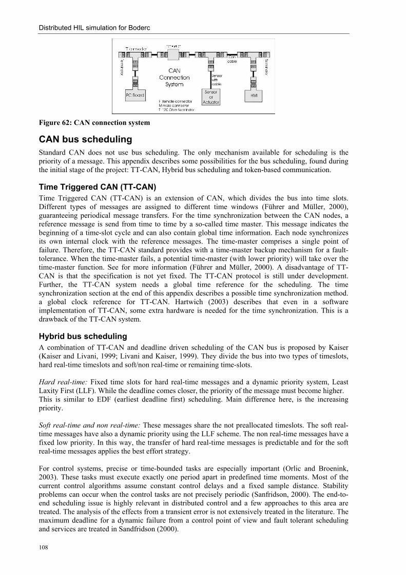
Distributed HIL simulation for Boderc
108
Figure 62: CAN connection system
CAN bus scheduling Standard CAN does not use bus scheduling. The only mechanism available for scheduling is the priority of a message. This appendix describes some possibilities for the bus scheduling, found during the initial stage of the project: TT-CAN, Hybrid bus scheduling and token-based communication.
Time Triggered CAN (TT-CAN) Time Triggered CAN (TT-CAN) is an extension of CAN, which divides the bus into time slots. Different types of messages are assigned to different time windows (Führer and Müller, 2000), guaranteeing periodical message transfers. For the time synchronization between the CAN nodes, a reference message is send from time to time by a so-called time master. This message indicates the beginning of a time-slot cycle and can also contain global time information. Each node synchronizes its own internal clock with the reference messages. The time-master comprises a single point of failure. Therefore, the TT-CAN standard provides with a time-master backup mechanism for a fault-tolerance. When the time-master fails, a potential time-master (with lower priority) will take over the time-master function. See for more information (Führer and Müller, 2000). A disadvantage of TT-CAN is that the specification is not yet fixed. The TT-CAN protocol is still under development. Further, the TT-CAN system needs a global time reference for the scheduling. The time synchronization section at the end of this appendix describes a possible time synchronization method. a global clock reference for TT-CAN. Hartwich (2003) describes that even in a software implementation of TT-CAN, some extra hardware is needed for the time synchronization. This is a drawback of the TT-CAN system.
Hybrid bus scheduling A combination of TT-CAN and deadline driven scheduling of the CAN bus is proposed by Kaiser (Kaiser and Livani, 1999; Livani and Kaiser, 1999). They divide the bus into two types of timeslots, hard real-time timeslots and soft/non real-time or remaining time-slots. Hard real-time: Fixed time slots for hard real-time messages and a dynamic priority system, Least Laxity First (LLF). While the deadline comes closer, the priority of the message must become higher. This is similar to EDF (earliest deadline first) scheduling. Main difference here, is the increasing priority. Soft real-time and non real-time: These messages share the not preallocated timeslots. The soft real-time messages have also a dynamic priority using the LLF scheme. The non real-time messages have a fixed low priority. In this way, the transfer of hard real-time messages is predictable and for the soft real-time messages applies the best effort strategy. For control systems, precise or time-bounded tasks are especially important (Orlic and Broenink, 2003). These tasks must execute exactly one period apart in predefined time moments. Most of the current control algorithms assume constant control delays and a fixed sample distance. Stability problems can occur when the control tasks are not precisely periodic (Sanfridson, 2000). The end-to-end scheduling issue is highly relevant in distributed control and a few approaches to this area are treated. The analysis of the effects from a transient error is not extensively treated in the literature. The maximum deadline for a dynamic failure from a control point of view and fault tolerant scheduling and services are treated in Sandfridson (2000).

Distributed HIL simulation for Boderc
109
Token Protocol Another option for CAN bus scheduling is a token rotation protocol. Every node can send only one message at a time and after that, the next node may send a message. When the node has nothing to send, it gives the token to the next node by sending an empty message. In fact, each message is a token passing message.
Advantages • Simple to implement • No babbling idiot problems (when all nodes behave well and send one message per round) • No global time reference required • No special token passing messages are needed when a node sends a data message • The worst case token rotation time (TTR) is predictable when assuming no retransmission of
messages after an error.
Disadvantages • Single point of failure: When the node that has the token, fails, the token is lost. Also, when
the next node in the ring does not receive the token message, the token is lost. Extra measures are needed to recover from such a failure.
• Token passing: CAN is a broadcast network; passing the token to the next node requires a receiver address. In CAN each node gets each token passing message but only one node should get the token.
• Waste of bandwidth: When a node gets the token and has nothing to send, it must at least send a 65 bit message (for CAN 2.0a: 47 bits (message with empty data field) across the CAN network to pass the token to the next node.
• Bandwidth: The maximum bus access time for all nodes is equal (max. one message, 154 bit times). Not possible to give one node more ‘time’ to send messages than others.
The token passing problem can be easily solved for CAN. It is possible to use the CAN arbitration field as a sender address, defining some of the bits as identification of the sending node. The receiving nodes should use these bits to check whether it is the next node in the token (filtering the token messages).
Timed Token Protocol An extension of the token protocol is the Timed Token Protocol (TTP). It is used on the Profibus and the 100 Mbit FDDI network (Hamdaoui, 1995). Although the Profibus is a master-slave bus, the idea of the timed token passing could be used for a CAN network. The idea behind the TTP is that each node knows the target token rotation time (TTR) and that each node measures the real token rotation time. After a node receives a token, the measurement of the real token rotation time begins. This measurement expires at the next token arrival and results in the real token rotation (TRR). When a node detects a difference between the target and real token time, that node knows that the token is too late or too early and can correct this by altering its own token holding time (THT), the time that a node may hold the token.
Advantages The advantages of TTP for usage on the CAN bus:
• No clock synchronization required, Each node uses only the own clock • Simple to implement. • Different (fixed) THT per node possible
Disadvantages The disadvantages with respect to TTP on CAN:
• Single point of failure: When the node that has the token, fails, the token ring is broken. Extra measures are needed to recover from such a failure

Distributed HIL simulation for Boderc
110
• Token passing: CAN is a broadcast network; passing the token to the next node requires a receiver address. In CAN each node gets each token passing message but only one node should respond to it.
Time synchronization For guaranteeing the transmission of hard-real-time messages over the CAN bus, Kaiser (2000) proposes a mechanism with fixed time-slots for hard-real-time messages. For this mechanism to work, time synchronization between the CAN nodes is necessary. Time triggered communication means that sending or receiving or any other activity depends on a predefined time schedule and on the current state of a ‘global’ system clock (Führer and Müller, 2000).
Figure 63: Scheduled message transfer
One possibility for the time synchronization is given in (Führer and Müller, 2000). This paper describes an extension of the standard CAN implementation called Time Triggered CAN (TT-CAN). See section 0 for more information about TTCAN. Another time synchronization method similar to the reference messages in TT-CAN was developed by Gergeleit and Streich (1994). They describe a clock synchronization protocol for the CAN-bus that provides a global time base with an accuracy of about 20 microseconds. Also here, there is one master clock. The other CAN nodes are slave nodes with adaptive clocks. When the master takes its current time and broadcasts it, all slaves receive the message and adjust their clocks taking into account the latency of the path between the master and the slave. The paper describes also the implementation and problems with the synchronization.

Distributed HIL simulation for Boderc
111
Appendix X: CTC++ versus PThreads This appendix shows the difference in the declaration of two parallel running threads under CT and with the use of PThreads. The PThreads solution requires some C++ to C wrapper code, because PThreads is C based and does not support class objects. Listing 11 shows the CTC++ solution and Listing 12 shows the PThreads solution and how to use PThreads for C++ classes. #include <stdio.h> // Include the csp include files #include "csp/lang/include/Parallel.h" #include "csp/lang/include/Process.h" #include "csp/lang/include/Channel.h" class ThreadProcess : public Process { public: ThreadProcess() {}; virtual ~ThreadProcess() {}; virtual void run(); }; int main(int argc, char *argv[]) { // Create the processes ThreadProcess *thread1 = new ThreadProcess(); ThreadProcess *thread2 = new ThreadProcess(); Process *par = new Parallel(thread1, thread2); // Start parallel threads par->run(); printf(“Done...\n”); delete thread1; delete thread2; delete par; return 0; } ThreadProcess::run() { printf("ThreadProcess::run: Entered the thread for object %p\n", this); }
Listing 11: Parallel CT threads
#define _MULTI_THREADED #include <stdio.h> #include <stdlib.h> #include <pthread.h> class ThreadClass { public: ThreadClass() {}; void *run(void); }; extern "C" void *ThreadStartup1(void *); extern "C" void *ThreadStartup2(void *); int main(int argc, char **argv) { ThreadClass *thread1 = new ThreadClass(); ThreadClass *thread2 = new ThreadClass(); //Start parallel threads:

Distributed HIL simulation for Boderc
112
pthread_t pthread1, pthread2; int rc; rc = pthread_create(&pthread1, NULL, ThreadStartup1, thread1); rc = pthread_create(&pthread2, NULL, ThreadStartup2, thread2); if (rc) { printf("Failed to create a thread\n"); exit(1); } printf("Waiting for threads to complete\n"); pthread_join(pthread1, NULL); pthread_join(pthread2, NULL); if (rc) { printf("ThreadClass::run: Failed to join to the thread, rc=%d\n"); exit(1); } printf("Done...\n"); delete thread1; delete thread2; return 0; } // This function is a helper function. It has normal C linkage, and is // as the base for newly created ThreadClass objects. It runs the // run method on the ThreadClass object passed to it (as a void *). // After the ThreadClass method completes normally (i.e returns), // we delete the object. void *ThreadStartup1(void *_tgtObject) { ThreadClass *tgtObject = (ThreadClass *)_tgtObject; printf("ThreadStartup1: Running thread object in a new thread\n"); tgtObject->run(); printf("ThreadStartup1: Return from thread\n"); return 0; } void *ThreadStartup2(void *_tgtObject) { ThreadClass *tgtObject = (ThreadClass *)_tgtObject; printf("ThreadStartup2: Running thread object in a new thread\n"); tgtObject->run(); printf("ThreadStartup2: Return from thread\n"); return 0 } void *ThreadClass::run(void) { printf("ThreadClass::run: Entered the thread for object %p\n", this); return 0; }
Listing 12: Parallel C++ threads in PThreads

Distributed HIL simulation for Boderc
113
References Andersen, E. (2004), uClibc website, http://www.uclibc.org. Berg, L.S.v.d. (2003), Design of a Virtual Engine for embedded software development, Océ
Technologies B.V., Venlo. Bosch (1991), CAN Specification version 2.0, Robert Bosch GmbH, Stuttgart, Cervin, A., D. Hendriksson, B. Lincoln and K.-E. Arzen (2002), Jitterbug and TrueTime: Analysis Tools for RealTime Control Systems, Proc. 2nd Workshop on RealTime Tools, Copenhagen, Denmark, (Ed.), pp. ISBN: CIA (2003), CAN Protocol, http://www.can-cia.de/can/protocol. Douglass, B.P. (1999), Doing Hard Time, Developing Real-Time Systems with UML, Objects,
Frameworks, and patterns, Addison Wesley Longman Inc., 0-201-49837-5. Engelschall, R.S. (2003), GNU Pth -The GNU Portable Threads (website),
http://www.gnu.org/software/pth/. Führer, T. and B. Müller (2000), Time Triggered Can,
http://www.can.bosch.com/content/Literature.html. Gergeleit, M. and H. Streich (1994), Implementing a Distributed High-Resolution Real-Time Clock
using the CAN-bus, Proc. 1st International CAN-Conference 94, Mainz, C. i. A. e. V. Erlangen (Ed.), pp. ISBN:
GNU (2001), GNU C Library reference manual, http://www.delorie.com/gnu/docs/glibc/libc.html#SEC_Top.
Groothuis, M.A. (2001), 20-sim code generation for PC/104 target, Individual Design Report, University of Twente, Enschede.
Hamdaoui, M. (1995), Selection of Timed Token Protocol Parameters to Guarantee Message Deadlines, IEEE/ACM Transactions on Networking, 3, (3), pp. ISSN:
Hartwich, F., B. Müller, T. Führer and R. Hugel (2003), Timing in the TTCAN Network, Robert Bosch GmbH,
Hilderink, G.H. (1997), Communicating Java Threads Reference Manual, Proc. Proc. WoTUG-20 on Parallel programming and Java, Enschede, Netherlands, (Ed.), pp. 283-325, ISBN: 1383-7575.
Hilderink, G.H. (2003), Graphical modelling language for specifying concurrency based on CSP, IEE Proceedings: Software, 150, (2), pp. 108-120, ISSN: 1462-5970
Hilderink, G.H., A.W.P. Bakkers and J.F. Broenink (2000), A Distributed Real-Time Java System Based on CSP, Proc. The third IEEE International Symposium on Object-Oriented Real-Time Distributed Computing ISORC 2000, Newport Beach, CA, (Ed.), pp. 400-407, ISBN:
Ho, J. (2003), Eden versus Crusoe, CPU comparison presentation, Proc. (Ed.), pp. ISBN: Hoare, C.A.R. (1985), Communicating Sequential Processes, Prentice Hall, 0-13-153271-5 (0-13-
153289-8 PBK). Isermann, R., J. Schaffnit and S. Sinsel (1998), Hardware-in-the-loop simulation for the design and
testing of engine control systems, Control Engineering Practice, 7, (5), pp. 643-653, ISSN: Kaiser, J. (2000), Real-time Communication on the CAN-bus for Distributed Applications with
Decentralized Control, Proc. 4th International Symposium on Intelligent Components and Instruments for Control Applications - SICICA 2000, Buenos Aires, Argentina, (Ed.), pp. ISBN:
Kaiser, J. and M.A. Livani (1999), Achieving Fault-Tolerant Ordered Broadcasts in CAN, Proc. European Dependable Computing Conference, J. Hlavicka (Ed.), pp. 351-363, ISBN:
Kaiser, J., M.A. Livani and W. Jia (2000), Predictability of Message Transfer in CSMA-Networks, Proc. International Conference on Algorithms and Architectures for Parallel Processing (ICA3PP2000), Hong Kong, China, (Ed.), pp. ISBN:
Kaiser, J. and M. Mock (1999), Implementing the Real-Time Publisher/Subscriber Model on the Controller Area Network (CAN), Proc. 2nd Int'l Symposium on ObjectOriented Distributed Real-Time Computing Systems,, San Malo, (Ed.), pp. ISBN:
Kopetz, H. (1997), Real-Time Systems, Design principles for Distributed Embedded Applications, Kluwer Academic Publishers, Boston, 0-7923-9894-7.

Distributed HIL simulation for Boderc
114
Krekels, S. (2002), Geode Processors versus Via Eden (webpage), https://mail.rtai.org/pipermail/rtai/2002-October/001207.html.
Livani, M.A. and J. Kaiser (1998), EDF Consensus on CAN Bus Access for Dynamic Real-Time Applications, Proc. 6th Int. Workshop on Parallel and Distributed Real-Time Systems (WPDRTS ´98), Orlando, FL,USA, (Ed.), pp. ISBN:
Livani, M.A. and J. Kaiser (1999), Evaluation of a Hybrid Real-time Bus Scheduling Mechanism for CAN, Lecture notes in Computer Science, 1586, pp. 425-429, ISSN:
Mocking, C. (2002), 20-sim code generation for ADSP-21990 EZ-KIT, Individual Design Assignment, Nolte, T., H. Hansson and C. Norström (2002), Minimizing CAN response-time jitter by message
manipulation, Proc. (Ed.), pp. ISBN: Orlic, B. and J.F. Broenink (2003), Real-time and fault tolerance in distributed control software, Proc.
Communicating Process Architectures 2003, 7 - 10 September 2003, Enschede, Netherlands, G. H. Hilderink (Ed.), pp. 235-250, ISBN: 1 58603 381 6.
Orlic, B., H. Ferdinando and J.F. Broenink (2003), CAN Fieldbus Communication in the CSP-based CT Library, Proc. PROGRESS 2003, Embedded Systems Symposium, 22 October 2003, F. Karelse (Ed.), pp. 163-171, ISBN: 90-73461-36-7.
Parchomov, L.J. (2002), Real Time Control on CAN, Individual Design Report, Control Laboratory, University of Twente,
Philips (2000), SJA1000 Stand-alone CAN controller (datasheet), PLX (2002), PCI 9030 Data Book, http://www.plxtech.com. Punnekkat, S. (2000), Response Time Analysis under Errors for CAN, Proc. RTAS'2000 6th IEEE
Real-Time Technology and Applications Symposium, June 2000, (Ed.), pp. 258-265, ISBN: Rubini, A. and J. Corbert (2001), Linux Device Drivers, 2nd Edition, O'Reilly and Associates Inc.,
Sebastopol, 0-596-00008-1. Sanfridson, M. (2000), Timing Problems in Distributed Real Time Computer Control Systems, Proc.
(Ed.), pp. ISBN: Sanvido, M.A.A. (2002), Hardware-in-the-loop simulation Framework, PhD, Automatic Control
Laboratory, ETH Zürich, Zürich. Stephan, R.A. (2002), Real-time Linux in Control Applications Area, MSc thesis 016CE2002, Dept.
Electrical Engineering, University of Twente, Enschede. Transmeta (2004), Transmeta Crusoe processor (website), http://www.transmeta.com/crusoe/. Via (2003), Via Embedded - Via Eden Platform (datasheet), http://www.viaembedded.com. Visser, P.M. and J.F. Broenink (2003), Group 4: Desciption of experimental set-up: Virtual Engine &
Distributed control, Internal Report, Embedded Systems Institute, Eindhoven. Xilinx (2004), Xilinx ISE Webpack & Modelsim XE, http://www.xilinx.com