University of Twente Business Administration Financial ...essay.utwente.nl/65105/1/Linderhof_MA_MB.pdf · University of Twente Business Administration ... Financial Management

University of Twente

Business Administration

Financial Management

“Does working capital management affect the profitability of

public listed firms in the Netherlands?”

J.H.C. Linderhof

I

Colophon

Master thesis title: “Does working capital management affect the profitability of public listed

firms in the Netherlands?”

Place and date: Enschede, May 2014

Amount of pages: 66

Appendices: 6

Filename: Linderhof_MA_MB.pdf

Status: Final version

Author: Johannes Hermanus Cornelius Linderhof

Student number: - privacy-sensitive data -

Address: - privacy-sensitive data -

Mail address: - privacy-sensitive data -

Phone number: - privacy-sensitive data -

Supervisory Committee:

1st Supervisor:

Ir. Henk Kroon

2nd Supervisor:

Dr. Peter Schuur

University of Twente

Faculty: School of Management and Governance

Study: Business Administration

Specialisation: Financial Management

Address: Drienerlolaan 5

7522 NB Enschede

Postal address: PO Box 217

7500 AE Enschede

Phone number: +31534899111

Mail address: [email protected]

Website: www.utwente.nl

II

Preface & acknowledgement

Although the thesis is written on an individual basis, I would like to thank the people around me for their

continuous faith, support in all kind of ways, encouragements and guidance through the whole research

period.

First of all, I want to thank my first supervisor Henk Kroon for all of his support, encouragements, his

professional perspective as well as his valuable advice and flexibility through the whole research period.

Besides Henk Kroon I would also like to thank my second supervisor Peter Schuur for his time and help in

the final stage of the research period. Besides both supervisors I want to thank Henry van Beusichem for

the time he invested to provide a critical but professional view on the statistical aspects of this research.

I am grateful to my parents, my family, my girlfriend Sanne Kreeftenberg, my parents-in-law, my colleagues

and friends for their faith, their support and the freedom I had while fullfilling my research. My roommates

for supporting me during the research project with all kind of daily activities during the research period

and the appropriate distraction on non-thesis moments. I would especially like to thank my roommate and

colleague student Jan-Jaap Meendering and colleague student Christian Verharen for the Sundays that we

have worked on our theses in the library, and Gerhard Kruiger for the conversations and support during

our journeys to the university in Enschede.

At last, I want to thank the Dutch government for their investments in my future and knowledge.

I hope you will enjoy reading this thesis.

Johannes H.C. Linderhof

May 2014

Enschede, the Netherlands

III

Table of contents Colophon ....................................................................................................................................................... I

Preface & acknowledgement ........................................................................................................................ II

Table of contents ......................................................................................................................................... III

Index of figures and tables .......................................................................................................................... IV

List of abbreviations .................................................................................................................................... V

Abstract ...................................................................................................................................................... VI

1. Introduction .......................................................................................................................................... 1

2. Literature review .................................................................................................................................. 2

2.1 Working Capital Management ........................................................................................................ 2

2.2 The Cash Conversion Cycle ............................................................................................................. 2

2.2.1 The number of days accounts receivable and firm profitability ................................................ 4

2.2.2 The number of days inventory and firm profitability ................................................................ 5

2.2.3 The number of days accounts payable and firm profitability ................................................... 6

2.3 Prior research ................................................................................................................................. 6

3. Hypotheses ......................................................................................................................................... 15

4. Methodology ...................................................................................................................................... 18

4.1 Variables ...................................................................................................................................... 18

4.1.1 Dependent variables.............................................................................................................. 18

4.1.2 Independent variables ........................................................................................................... 19

4.1.3 Control variables ................................................................................................................... 20

4.2 Research design ............................................................................................................................ 22

4.3 Data collection ............................................................................................................................. 25

5. Empirical Findings ............................................................................................................................... 26

5.1 Descriptive statistics ..................................................................................................................... 26

5.2 Correlation analysis ...................................................................................................................... 28

5.3 Regression analyses ...................................................................................................................... 30

5.3.1 OLS regressions with the dependent variable ROA: ............................................................... 31

5.3.2 FEM regressions with the dependent variable ROA: .............................................................. 34

5.3.3 OLS regressions with the dependent variable GOP: ............................................................... 36

5.3.4 GLS REM regressions with the dependent variable GOP: ....................................................... 39

5.4 Relationships ................................................................................................................................ 42

6. Conclusions ......................................................................................................................................... 47

Bibliography ............................................................................................................................................... 49

Appendices ................................................................................................................................................. 51

Appendix A1 ........................................................................................................................................... 51

Appendix A2 ........................................................................................................................................... 53

Appendix A3 ........................................................................................................................................... 55

Appendix A4 ........................................................................................................................................... 56

Appendix A5 ........................................................................................................................................... 57

Appendix A6 ........................................................................................................................................... 58

IV

Index of figures and tables Table 1: List of abbreviations ....................................................................................................................... V

Table 2: Different names for the Cash Conversion Cycle ............................................................................... 3

Table 3: Overview of found relationships by different authors .................................................................... 11

Table 4: Dependent variables and their calculations ................................................................................... 12

Table 5: Control variables and their calculations ......................................................................................... 14

Table 6: Overview of used regression models by different authors ............................................................. 22

Table 7: Number of firms per industry ........................................................................................................ 25

Table 8: Descriptive Statistics...................................................................................................................... 26

Table 9: Pearson Correlation Matrix (two-tailed) ........................................................................................ 29

Table 10: Overview Ordinary Least Squares regressions (dependent variable ROA) .................................... 33

Table 11: Overview Fixed-Effects Model regressions (dependent variable ROA) ......................................... 35

Table 12: Overview Ordinary Least Squares regressions (dependent variable GOP) .................................... 38

Table 13: Overview GLS Random-Effects Model regressions (dependent variable GOP) ............................. 41

Table 14: Overview relationships between variables .................................................................................. 42

V

List of abbreviations CCC = Cash Conversion Cycle

CG = Cash Gap

DWC = Days Working Capital

FEM = Fixed-Effects Model

GLS = Generalized Least Squares

GOI = Gross Operating Income

GOP = Gross Operating Profit

NOI = Net Operating Income

NOP = Net Operating Profitability

NTC = Net Trade Cycle

OLS = Ordinary Least Squares

REM = Random-Effects Model

ROA = Return on Assets

ROS = Return on Sales

ROTA = Return on Total Assets

VIF = Variance Inflation Factor

WCM = Working Capital Management

Table 1: List of abbreviations

VI

Abstract The objective of this research is to provide empirical evidence about the impact of Working Capital

Management (WCM) on the profitability of Dutch listed firms. This is considered to be of high importance

for firms to survive, because it has an effect on firm liquidity and firm profitability. Efficient Working Capital

refers to a proper trade-off between liquidity and profitability. To investigate the relationship between

WCM and the profitability of Dutch listed firms, the following research question for this research is drawn:

“�� ? ”

The effects of WCM on firm profitability are tested with the hypotheses as found below:

� Hypothesis 1: There is a negative relationship between the number of days accounts receivable and the

profitability of Dutch listed firms.

� Hypothesis 2: There is a negative relationship between the number of days inventory and the


� Hypothesis 3: There is a positive relationship between the number of days accounts payable and the


� Hypothesis 4: There is a negative relationship between the cash conversion cycle period and the


� Hypothesis 5: There is a negative relationship between the net trade cycle period and the profitability

of Dutch listed firms.

Furthermore, the effects of firm size, sales growth, current ratio, debt ratio and the annual GDP growth

rate on the profitability of Dutch listed firms are investigated.

The outcome of this research concludes that WCM does affect the profitability of the Dutch listed firms

used in this research. This is consistent with the outcome of the majority of other researches on this topic.

For these reasons the assumption can be made that the outcome of this research is applicable to future

research on this topic.

The data used in this research is a balanced panel dataset of 67 firms is collected through the ORBIS

database by Bureau van Dijk covering the period of nine years ranging from 2004-2012, resulting in a total

of 603 firm year observations.

To test the relationship between WCM and firm profitability, this research chose to test profitability

through Return on Assets and Gross Operating Profit as dependent variables. To test WCM the number of

days accounts receivable, the number of days inventory, the number of days accounts payable, the Cash

Conversion Cycle and the Net Trade Cycle are chosen as the independent variables. Furthermore, firm size,

sales growth, current ratio, debt ratio and GDP growth are chosen as the control variables.

The relationships are tested through a Pearson correlation, Ordinary Least Squares regressions with a

robust standard error, a Fixed-Effects regression model for the dependent variable Return on Assets and a

Random-Effects regression model for the dependent variable Gross Operating Profit. The Ordinary Least

Squares regressions are tested on the presence of multicollinearity and heteroskedasticity.

A Hausman test is performed to determine whether the Fixed-Effects regression model or the Random-

Effects regression model is the appropriate regression model for the dependent variables Return on Assets

and Gross Operating Profit.

The found relationships indicate a negative and significant relationship between the number of days

accounts receivable and profitability, a negative and significant relationship between the number of days

inventory and profitability, a negative and significant relationship between the number of days accounts

VII

payable and profitability, a negative and significant relationship between the Cash Conversion Cycle period

and profitability and a negative and significant relationship between the Net Trade Cycle period and

profitability.

The research is a repetition of existing research, but is rather unique due to testing profitability with two

different dependent variables and by choosing both Cash Conversion Cycle and Net Trade Cycle as

independent variables. Having a greater variety of variables makes this research more complex and

simultaneously it makes this research more comparable to other existing research. Because of these

reasons this research contributes to the validity of a greater amount of existing research than other

researches on the same topic. Furthermore, this research focuses on Dutch listed firms where limited

research has been done to test the relationship between WCM and firm profitability.

This research contains a limited amount of Dutch listed firms due to the unavailability of data. Financial

orientated firms and SME’s are taken out of the dataset, this makes this research not generalizable to all

firms. It is tried to find a relationship between WCM and firm profitability, and it does not discuss an

optimum level for WCM.

Key words*: Working Capital Management, Firm Profitability, Return on Assets, Gross Operating Profit,

Cash Conversion Cycle, Net Trade Cycle, the number of days Accounts Receivable, the number of days

Inventory, the number of days Accounts Payable, Firm Size, Sales Growth, Current Ratio, Debt Ratio, Gross

Domestic Product Growth, Pearson Correlation, Ordinary Least Squares, Variance Inflation Factor,

Multicollinearity, White’s test, Heteroskedasticity, Robust Standard Error, Fixed-Effects Model, Generalized

Least Squares Random-Effects Model, Hausman Test.

* The listed key words are related to the content (subjects of research) and to the theory (research methods used). The listed key

words should provide the reader with a quick and stepwise overview of the research.

1

1. Introduction

Working Capital Management (WCM) is considered to be of high importance for firms to survive, because

it has an effect on firm liquidity and firm profitability. It refers to the management of working capital which

is the sum of current assets minus current liabilities, and good WCM refers to a proper trade-off between

liquidity and profitability. The current assets are accounts receivable and inventory, and the current

liabilities are accounts payable.

The goal of this research is to find a relationship between WCM and firm profitability over a period of 9

years for 67 Dutch listed firms. WCM will be investigated through the CCC and NTC period, and the

individual components: the number of days inventory, the number of days accounts receivable and the

number of days accounts payable.

As far as I know there is no similar research done on the relationship between working capital

management and the profitability of Dutch listed firms. This research will provide information for Dutch

listed firms on how to manage their working capital. In other words, how to plan their policies towards

inventory management, credit management and financing management.

The research question for this research:

“�� ? ”

To prove the effects of WCM on firm profitability, this research will use a hypothesis testing approach.

The following hypotheses are drawn:

� Hypothesis 1: There is a negative relationship between the number of days accounts receivable and the


� Hypothesis 2: There is a negative relationship between the number of days inventory and the


� Hypothesis 3: There is a positive relationship between the number of days accounts payable and the


� Hypothesis 4: There is a negative relationship between the cash conversion cycle period and the


� Hypothesis 5: There is a negative relationship between the net trade cycle period and the profitability


The hypotheses are consistent with the findings of the majority of the prior research on the relationship

between WCM and firm profitability. Furthermore, the effects of firm size, sales growth, current ratio, debt

ratio and the annual GDP growth rate on the profitability of Dutch listed firms are investigated.

The research question and the related hypotheses will be analysed during this research using a correlation

and regressions. Hopefully the outcomes provide an useful contribution to the existing knowledge on

WCM, which is known to be an important aspect of Financial Management.

The next section discusses WCM in general and provides an overview of prior research on the relationship

between a firm’s WCM and profitability. Section three presents the conducted hypotheses for this

research. Section four discusses the research methodology and is divided in variables, research design and

data. Section five discusses the empirical findings on the correlation and regression analysis. Section six

gives a conclusion on the findings of this research.

2

2. Literature review 2.1 Working Capital Management In the past decade a large amount of articles have been written about the relationship between Working

Capital Management (WCM) and the profitability of firms. Most of the conducted studies report a negative

relationship between WCM and firm profitability (Jose et al., 1996; Shin and Soenen, 1998; Deloof, 2003;

Eljelly, 2004; Lazaridis and Tryfonidis, 2006; Padachi, 2006; García-Teruel and Martínez-Solano, 2007;

Raheman and Nasr, 2007; Uyar, 2009; Mathuva, 2010; Alipour, 2011; Ashraf, 2012; Kaddumi and Ramadan,

2012; Majeed et al., 2013). Conversely some studies found a positive relationship (Gill et al., 2010; Ching et

al., 2011; Sharma and Kumar, 2011; Baños-Caballero et al., 2012; Charitou et al., 2012) or no significant

relationship (Afeef, 2011) between WCM and firm profitability. WCM, which deals with managing a firms

current assets and current liabilities, is very important in corporate finance because it directly affects firm

profitability and firm liquidity (Deloof, 2003; Eljelly, 2004; Raheman and Nasr, 2007; Mathuva, 2010).

Net working Capital is defined as current assets minus current liabilities (Smith, 1980). Current assets can

be found on the left side of the balance sheet, and current liabilities can be found on the right side of the

balance sheet. Current assets refer to cash or cash equivalent, financial assets held for trading purposes

and operating assets which can be converted into cash within one year, and current liabilities are cash

requiring obligations to be fulfilled within one year (Sutton, 2004). WCM refers to using a firms current

assets, current liabilities and the interrelationships between them in an efficient way (Smith, 1980; Knauer

and Wöhrmann, 2013) and the day-to-day management of short term assets and liabilities is related to the

success of a firm (Jose et al., 1996). If the management towards working capital is incorrect, sales and

consequently firm profitability might decrease, and the firm may not be able to pay off its debts on time

(Alipour, 2011). In other words, WCM can have an impact on the profitability and liquidity of firms. Smith

(1980) found that a balance between both goals is important, this is called a trade-off. Trade-off between

profitability and liquidity is important for firms to survive. Firms focusing on maximizing profitability will

most likely reduce the liquidity of the firm and conversely; firms focusing on maximizing liquidity will most

likely reduce the profitability of the firm (Shin and Soenen, 1998). This is emphasized by (Baños-Caballero

et al., 2012) who state that a more aggressive approach towards WCM, which means a low investment in

working capital, is associated with higher return and risk. A more conservative approach towards WCM,

which means a high investment in working capital, is associated with lower return and risk. With an

aggressive approach towards WCM, the outcome of current assets minus current liabilities will be

negative. This means that the firm does not need external financing to finance the assets. With a

conservative approach towards WCM, the outcome of current assets minus current liabilities will be

positive. This means that the firm does need external financing to finance the assets, otherwise it could

encounter difficulties in paying its short-term debts. Not all firms are able to find external financing easily,

and the cost of external financing may be expensive, which could decrease firm profitability (Uyar, 2009).

There exist two types of methods for measuring WCM; the static and dynamic method. The static method

is based on liquidity ratios. The most conventional and commonly used liquidity measures are the current

ratio (CR) and the quick ratio (QR), which are based on the data of a firm’s balance sheet and measures

liquidity on some point in time. The dynamic method is based on the operations of a firm. The Cash

Conversion Cycle is a dynamic measurement method of ongoing liquidity management and combines the

data of a firm’s balance sheet and income statement and measures liquidity with a time dimension (Jose et

al., 1996; Uyar, 2009; Majeed et al., 2013). In the next paragraph, the Cash Conversion Cycle will be

explained.

2.2 The Cash Conversion Cycle The most popular measure for WCM is the Cash Conversion Cycle (CCC). Gitman (1974) introduced the

Cash Cycle, which is calculated by the number of days between obtaining inventory and collecting accounts

receivable. Richards and Laughlin (1980) adjusted the Cash Cycle by subtracting the number of days

accounts payable to get the CCC. The CCC is a dynamic measure of ongoing liquidity management that

3

combines data from the balance sheet and income statement to create a time dimension measurement

(Jose et al., 1996; Uyar, 2009; Majeed et al., 2013) and replaces the traditional liquidity ratios as CR and QR

which besides financial assets also include not useful operating assets in their formulas (Eljelly, 2004). The

CCC focuses on the time span between the expenditure for purchasing resources and the collection of cash

of goods sold (Shin and Soenen, 1998; Deloof, 2003; Eljelly, 2004; Lazaridis and Tryfonidis, 2006; Padachi,

2006; Raheman and Nasr, 2007; Uyar, 2009; Gill et al., 2010; Sharma and Kumar, 2011; Ashraf, 2012;

Majeed et al., 2013). The goods sold can be products and/or services, and resources can be raw materials,

labour and/or utilities.

Some of the authors have different names for the CCC, these are given in table 2 below.

Author(s): Name:

Gitman (1974) Cash Cycle (CC)

Richards and Laughlin (1980) Cash Conversion Cycle (CCC)

Shin and Soenen (1998) Net Trade Cycle (NTC)

Eljelly (2004) Cash Gap (CG)

Ching et al. (2011) Days of Working Capital (DWC)

Table 2: Different names for the Cash Conversion Cycle

A large portion of the reviewed literature used the CCC as a measurement for WCM (Jose et al., 1996;

Deloof, 2003; Eljelly, 2004; Lazaridis and Tryfonidis, 2006; Padachi, 2006; García-Teruel and Martínez-

Solano, 2007; Raheman and Nasr, 2007; Uyar, 2009; Gill et al., 2010; Mathuva, 2010; Afeef, 2011; Alipour,

2011; Sharma and Kumar, 2011; Ashraf, 2012; Baños-Caballero et al., 2012; Majeed et al., 2013), and a

noticeable smaller portion used the NTC (Shin and Soenen, 1998) or both CCC and NTC as a measurement

for WCM (Ching et al., 2011; Charitou et al., 2012; Kaddumi and Ramadan, 2012).

According to Shin and Soenen (1998) the Net Trade Cycle (NTC) is comparable with the CCC, the difference

between both is that the components of the CCC are expressed in the number of days, while the NTC

components are expressed in a percentage of net sales.

The components of the CCC are the number of days accounts receivable (DAR), the number of days

inventory (DI) and the number of days accounts payable (DAP), and are used as measures of trade credit

and inventory policies (Deloof, 2003). DAR and DI are parts of a firms current assets, and DAP is part of a

firms current liabilities. The calculations are as follow:

The number of days accounts receivable, calculated by1:

�� = �!�� !��"�� #�� $ ∗ &'(

The number of days inventory, calculated by2:

�) = �!�� )�!�� *�� #�� $ ∗ &'(

1 See Leach and Melicher (2011), p. 162-163 2 See Leach and Melicher (2011), p. 162

4

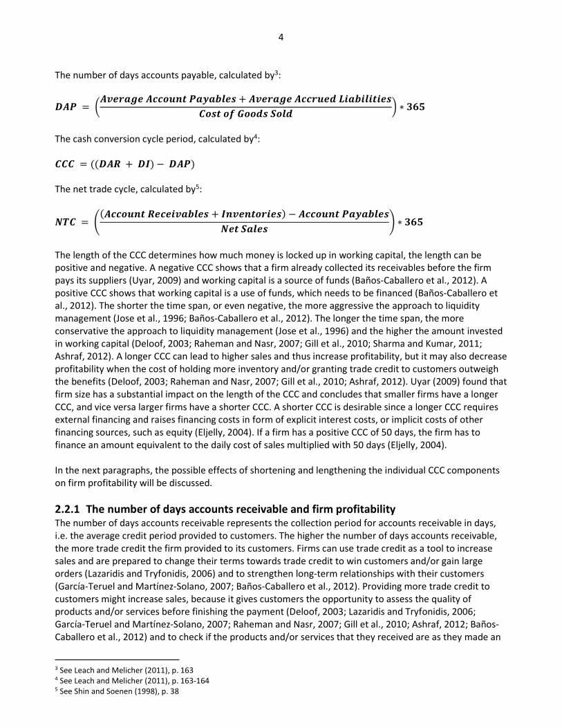
The number of days accounts payable, calculated by3:

��+ = �!�� +�� + �!�� -�� *�� #�� $ ∗ &'(

The cash conversion cycle period, calculated by4:

= ((�� + �)) − ��+)

The net trade cycle, calculated by5:

"1 = 2(�� !�� + )�!��) − �� +��"�� #�� 3 ∗ &'(

The length of the CCC determines how much money is locked up in working capital, the length can be

positive and negative. A negative CCC shows that a firm already collected its receivables before the firm

pays its suppliers (Uyar, 2009) and working capital is a source of funds (Baños-Caballero et al., 2012). A

positive CCC shows that working capital is a use of funds, which needs to be financed (Baños-Caballero et

al., 2012). The shorter the time span, or even negative, the more aggressive the approach to liquidity

management (Jose et al., 1996; Baños-Caballero et al., 2012). The longer the time span, the more

conservative the approach to liquidity management (Jose et al., 1996) and the higher the amount invested

in working capital (Deloof, 2003; Raheman and Nasr, 2007; Gill et al., 2010; Sharma and Kumar, 2011;

Ashraf, 2012). A longer CCC can lead to higher sales and thus increase profitability, but it may also decrease

profitability when the cost of holding more inventory and/or granting trade credit to customers outweigh

the benefits (Deloof, 2003; Raheman and Nasr, 2007; Gill et al., 2010; Ashraf, 2012). Uyar (2009) found that

firm size has a substantial impact on the length of the CCC and concludes that smaller firms have a longer

CCC, and vice versa larger firms have a shorter CCC. A shorter CCC is desirable since a longer CCC requires

external financing and raises financing costs in form of explicit interest costs, or implicit costs of other

financing sources, such as equity (Eljelly, 2004). If a firm has a positive CCC of 50 days, the firm has to

finance an amount equivalent to the daily cost of sales multiplied with 50 days (Eljelly, 2004).

In the next paragraphs, the possible effects of shortening and lengthening the individual CCC components

on firm profitability will be discussed.

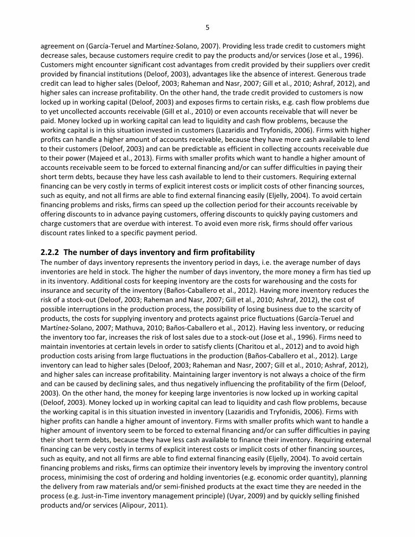
2.2.1 The number of days accounts receivable and firm profitability The number of days accounts receivable represents the collection period for accounts receivable in days,

i.e. the average credit period provided to customers. The higher the number of days accounts receivable,

the more trade credit the firm provided to its customers. Firms can use trade credit as a tool to increase

sales and are prepared to change their terms towards trade credit to win customers and/or gain large

orders (Lazaridis and Tryfonidis, 2006) and to strengthen long-term relationships with their customers

(García-Teruel and Martínez-Solano, 2007; Baños-Caballero et al., 2012). Providing more trade credit to

customers might increase sales, because it gives customers the opportunity to assess the quality of

products and/or services before finishing the payment (Deloof, 2003; Lazaridis and Tryfonidis, 2006;

García-Teruel and Martínez-Solano, 2007; Raheman and Nasr, 2007; Gill et al., 2010; Ashraf, 2012; Baños-

Caballero et al., 2012) and to check if the products and/or services that they received are as they made an

3 See Leach and Melicher (2011), p. 163 4 See Leach and Melicher (2011), p. 163-164 5 See Shin and Soenen (1998), p. 38

5

agreement on (García-Teruel and Martínez-Solano, 2007). Providing less trade credit to customers might

decrease sales, because customers require credit to pay the products and/or services (Jose et al., 1996).

Customers might encounter significant cost advantages from credit provided by their suppliers over credit

provided by financial institutions (Deloof, 2003), advantages like the absence of interest. Generous trade

credit can lead to higher sales (Deloof, 2003; Raheman and Nasr, 2007; Gill et al., 2010; Ashraf, 2012), and

higher sales can increase profitability. On the other hand, the trade credit provided to customers is now

locked up in working capital (Deloof, 2003) and exposes firms to certain risks, e.g. cash flow problems due

to yet uncollected accounts receivable (Gill et al., 2010) or even accounts receivable that will never be

paid. Money locked up in working capital can lead to liquidity and cash flow problems, because the

working capital is in this situation invested in customers (Lazaridis and Tryfonidis, 2006). Firms with higher

profits can handle a higher amount of accounts receivable, because they have more cash available to lend

to their customers (Deloof, 2003) and can be predictable as efficient in collecting accounts receivable due

to their power (Majeed et al., 2013). Firms with smaller profits which want to handle a higher amount of

accounts receivable seem to be forced to external financing and/or can suffer difficulties in paying their

short term debts, because they have less cash available to lend to their customers. Requiring external

financing can be very costly in terms of explicit interest costs or implicit costs of other financing sources,

such as equity, and not all firms are able to find external financing easily (Eljelly, 2004). To avoid certain

financing problems and risks, firms can speed up the collection period for their accounts receivable by

offering discounts to in advance paying customers, offering discounts to quickly paying customers and

charge customers that are overdue with interest. To avoid even more risk, firms should offer various

discount rates linked to a specific payment period.

2.2.2 The number of days inventory and firm profitability The number of days inventory represents the inventory period in days, i.e. the average number of days

inventories are held in stock. The higher the number of days inventory, the more money a firm has tied up

in its inventory. Additional costs for keeping inventory are the costs for warehousing and the costs for

insurance and security of the inventory (Baños-Caballero et al., 2012). Having more inventory reduces the

risk of a stock-out (Deloof, 2003; Raheman and Nasr, 2007; Gill et al., 2010; Ashraf, 2012), the cost of

possible interruptions in the production process, the possibility of losing business due to the scarcity of

products, the costs for supplying inventory and protects against price fluctuations (García-Teruel and

Martínez-Solano, 2007; Mathuva, 2010; Baños-Caballero et al., 2012). Having less inventory, or reducing

the inventory too far, increases the risk of lost sales due to a stock-out (Jose et al., 1996). Firms need to

maintain inventories at certain levels in order to satisfy clients (Charitou et al., 2012) and to avoid high

production costs arising from large fluctuations in the production (Baños-Caballero et al., 2012). Large

inventory can lead to higher sales (Deloof, 2003; Raheman and Nasr, 2007; Gill et al., 2010; Ashraf, 2012),

and higher sales can increase profitability. Maintaining larger inventory is not always a choice of the firm

and can be caused by declining sales, and thus negatively influencing the profitability of the firm (Deloof,

2003). On the other hand, the money for keeping large inventories is now locked up in working capital

(Deloof, 2003). Money locked up in working capital can lead to liquidity and cash flow problems, because

the working capital is in this situation invested in inventory (Lazaridis and Tryfonidis, 2006). Firms with

higher profits can handle a higher amount of inventory. Firms with smaller profits which want to handle a

higher amount of inventory seem to be forced to external financing and/or can suffer difficulties in paying

their short term debts, because they have less cash available to finance their inventory. Requiring external

financing can be very costly in terms of explicit interest costs or implicit costs of other financing sources,

such as equity, and not all firms are able to find external financing easily (Eljelly, 2004). To avoid certain

financing problems and risks, firms can optimize their inventory levels by improving the inventory control

process, minimising the cost of ordering and holding inventories (e.g. economic order quantity), planning

the delivery from raw materials and/or semi-finished products at the exact time they are needed in the

process (e.g. Just-in-Time inventory management principle) (Uyar, 2009) and by quickly selling finished

products and/or services (Alipour, 2011).

6

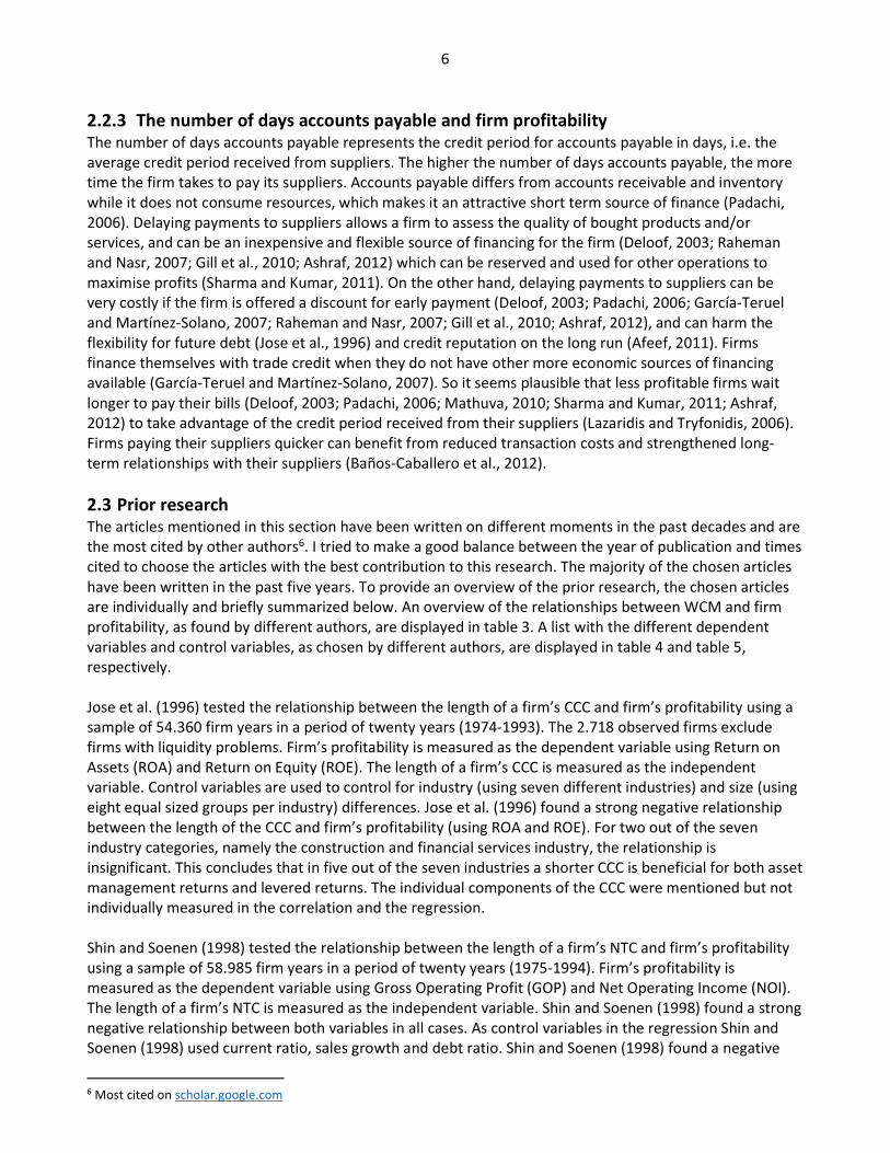
2.2.3 The number of days accounts payable and firm profitability The number of days accounts payable represents the credit period for accounts payable in days, i.e. the

average credit period received from suppliers. The higher the number of days accounts payable, the more

time the firm takes to pay its suppliers. Accounts payable differs from accounts receivable and inventory

while it does not consume resources, which makes it an attractive short term source of finance (Padachi,

2006). Delaying payments to suppliers allows a firm to assess the quality of bought products and/or

services, and can be an inexpensive and flexible source of financing for the firm (Deloof, 2003; Raheman

and Nasr, 2007; Gill et al., 2010; Ashraf, 2012) which can be reserved and used for other operations to

maximise profits (Sharma and Kumar, 2011). On the other hand, delaying payments to suppliers can be

very costly if the firm is offered a discount for early payment (Deloof, 2003; Padachi, 2006; García-Teruel

and Martínez-Solano, 2007; Raheman and Nasr, 2007; Gill et al., 2010; Ashraf, 2012), and can harm the

flexibility for future debt (Jose et al., 1996) and credit reputation on the long run (Afeef, 2011). Firms

finance themselves with trade credit when they do not have other more economic sources of financing

available (García-Teruel and Martínez-Solano, 2007). So it seems plausible that less profitable firms wait

longer to pay their bills (Deloof, 2003; Padachi, 2006; Mathuva, 2010; Sharma and Kumar, 2011; Ashraf,

2012) to take advantage of the credit period received from their suppliers (Lazaridis and Tryfonidis, 2006).

Firms paying their suppliers quicker can benefit from reduced transaction costs and strengthened long-

term relationships with their suppliers (Baños-Caballero et al., 2012).

2.3 Prior research The articles mentioned in this section have been written on different moments in the past decades and are

the most cited by other authors6. I tried to make a good balance between the year of publication and times

cited to choose the articles with the best contribution to this research. The majority of the chosen articles

have been written in the past five years. To provide an overview of the prior research, the chosen articles

are individually and briefly summarized below. An overview of the relationships between WCM and firm

profitability, as found by different authors, are displayed in table 3. A list with the different dependent

variables and control variables, as chosen by different authors, are displayed in table 4 and table 5,

respectively.

Jose et al. (1996) tested the relationship between the length of a firm’s CCC and firm’s profitability using a

sample of 54.360 firm years in a period of twenty years (1974-1993). The 2.718 observed firms exclude

firms with liquidity problems. Firm’s profitability is measured as the dependent variable using Return on

Assets (ROA) and Return on Equity (ROE). The length of a firm’s CCC is measured as the independent

variable. Control variables are used to control for industry (using seven different industries) and size (using

eight equal sized groups per industry) differences. Jose et al. (1996) found a strong negative relationship

between the length of the CCC and firm’s profitability (using ROA and ROE). For two out of the seven

industry categories, namely the construction and financial services industry, the relationship is

insignificant. This concludes that in five out of the seven industries a shorter CCC is beneficial for both asset

management returns and levered returns. The individual components of the CCC were mentioned but not

individually measured in the correlation and the regression.

Shin and Soenen (1998) tested the relationship between the length of a firm’s NTC and firm’s profitability

using a sample of 58.985 firm years in a period of twenty years (1975-1994). Firm’s profitability is

measured as the dependent variable using Gross Operating Profit (GOP) and Net Operating Income (NOI).

The length of a firm’s NTC is measured as the independent variable. Shin and Soenen (1998) found a strong

negative relationship between both variables in all cases. As control variables in the regression Shin and

Soenen (1998) used current ratio, sales growth and debt ratio. Shin and Soenen (1998) found a negative

6 Most cited on scholar.google.com

7

relationship between the NTC and firm’s profitability. The individual components of the NTC were

mentioned but not individually measured in the correlation and the regression.

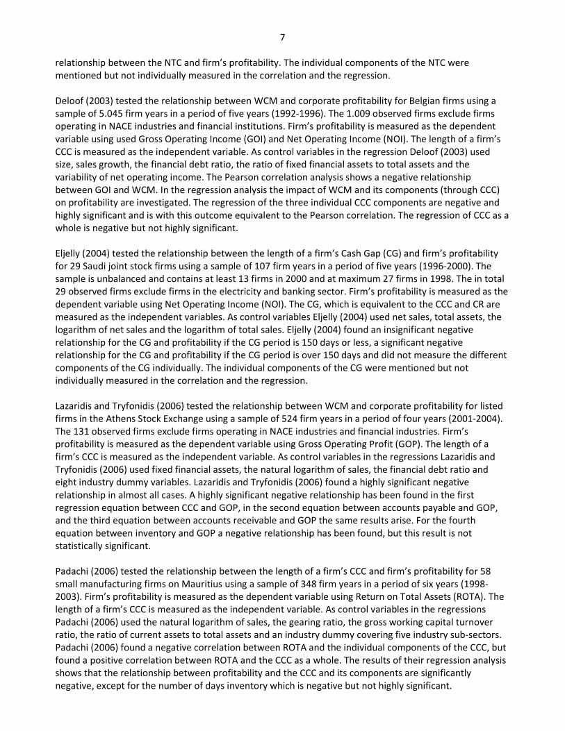
Deloof (2003) tested the relationship between WCM and corporate profitability for Belgian firms using a

sample of 5.045 firm years in a period of five years (1992-1996). The 1.009 observed firms exclude firms

operating in NACE industries and financial institutions. Firm’s profitability is measured as the dependent

variable using used Gross Operating Income (GOI) and Net Operating Income (NOI). The length of a firm’s

CCC is measured as the independent variable. As control variables in the regression Deloof (2003) used

size, sales growth, the financial debt ratio, the ratio of fixed financial assets to total assets and the

variability of net operating income. The Pearson correlation analysis shows a negative relationship

between GOI and WCM. In the regression analysis the impact of WCM and its components (through CCC)

on profitability are investigated. The regression of the three individual CCC components are negative and

highly significant and is with this outcome equivalent to the Pearson correlation. The regression of CCC as a

whole is negative but not highly significant.

Eljelly (2004) tested the relationship between the length of a firm’s Cash Gap (CG) and firm’s profitability

for 29 Saudi joint stock firms using a sample of 107 firm years in a period of five years (1996-2000). The

sample is unbalanced and contains at least 13 firms in 2000 and at maximum 27 firms in 1998. The in total

29 observed firms exclude firms in the electricity and banking sector. Firm’s profitability is measured as the

dependent variable using Net Operating Income (NOI). The CG, which is equivalent to the CCC and CR are

measured as the independent variables. As control variables Eljelly (2004) used net sales, total assets, the

logarithm of net sales and the logarithm of total sales. Eljelly (2004) found an insignificant negative

relationship for the CG and profitability if the CG period is 150 days or less, a significant negative

relationship for the CG and profitability if the CG period is over 150 days and did not measure the different

components of the CG individually. The individual components of the CG were mentioned but not

individually measured in the correlation and the regression.

Lazaridis and Tryfonidis (2006) tested the relationship between WCM and corporate profitability for listed

firms in the Athens Stock Exchange using a sample of 524 firm years in a period of four years (2001-2004).

The 131 observed firms exclude firms operating in NACE industries and financial industries. Firm’s

profitability is measured as the dependent variable using Gross Operating Profit (GOP). The length of a

firm’s CCC is measured as the independent variable. As control variables in the regressions Lazaridis and

Tryfonidis (2006) used fixed financial assets, the natural logarithm of sales, the financial debt ratio and

eight industry dummy variables. Lazaridis and Tryfonidis (2006) found a highly significant negative

relationship in almost all cases. A highly significant negative relationship has been found in the first

regression equation between CCC and GOP, in the second equation between accounts payable and GOP,

and the third equation between accounts receivable and GOP the same results arise. For the fourth

equation between inventory and GOP a negative relationship has been found, but this result is not

statistically significant.

Padachi (2006) tested the relationship between the length of a firm’s CCC and firm’s profitability for 58

small manufacturing firms on Mauritius using a sample of 348 firm years in a period of six years (1998-

2003). Firm’s profitability is measured as the dependent variable using Return on Total Assets (ROTA). The

length of a firm’s CCC is measured as the independent variable. As control variables in the regressions

Padachi (2006) used the natural logarithm of sales, the gearing ratio, the gross working capital turnover

ratio, the ratio of current assets to total assets and an industry dummy covering five industry sub-sectors.

Padachi (2006) found a negative correlation between ROTA and the individual components of the CCC, but

found a positive correlation between ROTA and the CCC as a whole. The results of their regression analysis

shows that the relationship between profitability and the CCC and its components are significantly

negative, except for the number of days inventory which is negative but not highly significant.

8

García-Teruel and Martínez-Solano (2007) tested the relationship between the length of a firm’s CCC and

firm’s profitability for 8.872 small and medium-sized Spanish firms using an unbalanced sample of 38.464

firm years in a period of seven years (1996-2002). Firm’s profitability is measured as the dependent

variable using Return on Assets (ROA). The length of a firm’s CCC and its components are measured as the

independent variables. As control variables García-Teruel and Martínez-Solano (2007) used the logarithm

of assets, sales growth, debt ratio and the GDP growth. García-Teruel and Martínez-Solano (2007) found a

negative relationship between ROA, the CCC and the individual CCC components. For the CCC, the number

of days accounts receivable and the number of days inventory this negative relationship is significant. For

the number of days accounts payable this relationship is not significant, but negative.

Raheman and Nasr (2007) tested the relationship between WCM and firm’s profitability for 94 Pakistani

firms listed on the Karachi Stock Exchange using a sample of 564 firm years in a period of six years (1999-

2004). Firm’s profitability is measured as the dependent variable using Net Operating Profitability (NOP).

The length of a firm’s CCC and its components, and the current ratio of a firm are measured as the

independent variables. The current ratio is used to measure the liquidity of a firm. As control variables in

the regressions Raheman and Nasr (2007) used firm size, debt ratio and the ratio of financial assets to total

assets. Raheman and Nasr (2007) found a significant negative relationship in all cases.

Uyar (2009) tested the relationship between the length of a firm’s CCC and the firm’s size, and the length

of a firm’s CCC and firm’s profitability for 166 Turkish firms listed on the Istanbul Stock Exchange in the

year 2007. Firm’s size is measured as the dependent variable by total assets and sales revenue, and firm’s

profitability is measured as the dependent variable using ROA and ROE. The length of a firm’s CCC and its

components are measured as the independent variables. As a control variable Uyar (2009) used the type of

industry. Uyar (2009) found a significant negative correlation between a firm’s CCC and a firm’s size for

both of the used measurements, found a significant negative correlation between a firm’s CCC and a firm’s

profitability measured with ROA and found no significant correlation between a firm’s CCC and a firm’s

profitability measured with ROE. The individual components of the CCC were mentioned but not

individually measured in the correlation.

Gill et al. (2010) tested the relationship between WCM and firm’s profitability for 88 American

manufacturing firms listed on the New York Stock Exchange using a sample of 264 firm years in a period of

three years (2005-2007). Firm’s profitability is measured as the dependent variable using used Gross

Operating Profit (GOP). The length of a firm’s CCC and its individual components are measured as the

independent variables. As control variables in the regressions Gill et al. (2010) used firm size, financial debt

ratio and fixed financial asset ratio. Gill et al. (2010) found a negative relationship between the number of

days accounts receivable and profitability, no significant relationship between the number of days

accounts payable and profitability, no significant relationship between the number of days inventory and

profitability and a positive relationship between the CCC and profitability.

Mathuva (2010) tested the relationship between WCM components and corporate profitability for 30

Kenyan firms listed on the Nairobi Stock Exchange using a sample of 468 firm years in a period of fifteen

years (1993-2008). Firm’s profitability is measured as the dependent variable using Net Operating Profit

(NOP). The length of a firm’s CCC and its individual components are measured as the independent variable.

As control variables in the regressions Mathuva (2010) used firm size, sales, leverage ratio, fixed financial

assets ratio, growth (using the growth in the gross domestic product) and the age of the firm. Mathuva

(2010) found a negative relationship between the number of days accounts receivable and profitability, a

positive relationship between the number of days inventory and profitability, a positive relationship

between the number of days accounts payable and profitability and a negative relationship between the

CCC and profitability.

9

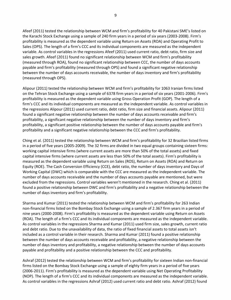
Afeef (2011) tested the relationship between WCM and firm’s profitability for 40 Pakistani SME’s listed on

the Karachi Stock Exchange using a sample of 240 firm years in a period of six years (2003-2008). Firm’s

profitability is measured as the dependent variable using Return on Assets (ROA) and Operating Profit to

Sales (OPS). The length of a firm’s CCC and its individual components are measured as the independent

variable. As control variables in the regressions Afeef (2011) used current ratio, debt ratio, firm size and

sales growth. Afeef (2011) found no significant relationship between WCM and firm’s profitability

(measured through ROA), found no significant relationship between CCC, the number of days accounts

payable and firm’s profitability (measured through OPS) and found a significant negative relationship

between the number of days accounts receivable, the number of days inventory and firm’s profitability

(measured through OPS).

Alipour (2011) tested the relationship between WCM and firm’s profitability for 1063 Iranian firms listed

on the Tehran Stock Exchange using a sample of 6378 firm years in a period of six years (2001-2006). Firm’s

profitability is measured as the dependent variable using Gross Operation Profit (GOP). The length of a

firm’s CCC and its individual components are measured as the independent variable. As control variables in

the regressions Alipour (2011) used current ratio, debt ratio, firm size and financial assets. Alipour (2011)

found a significant negative relationship between the number of days accounts receivable and firm’s

profitability, a significant negative relationship between the number of days inventory and firm’s

profitability, a significant positive relationship between the number of days accounts payable and firm’s

profitability and a significant negative relationship between the CCC and firm’s profitability.

Ching et al. (2011) tested the relationship between WCM and firm’s profitability for 32 Brazilian listed firms

in a period of five years (2005-2009). The 32 firms are divided in two equal groups containing sixteen firms:

working capital intensive firms (where current assets are more than 50% of the total assets) and fixed

capital intensive firms (where current assets are less than 50% of the total assets). Firm’s profitability is

measured as the dependent variable using Return on Sales (ROS), Return on Assets (ROA) and Return on

Equity (ROE). The Cash Conversion Efficiency (CCE), debt ratio, the number of days inventory and Days of

Working Capital (DWC) which is comparable with the CCC are measured as the independent variable. The

number of days accounts receivable and the number of days accounts payable are mentioned, but were

excluded from the regressions. Control variables weren’t mentioned in the research. Ching et al. (2011)

found a positive relationship between DWC and firm’s profitability and a negative relationship between the

number of days inventory and firm’s profitability.

Sharma and Kumar (2011) tested the relationship between WCM and firm’s profitability for 263 Indian

non-financial firms listed on the Bombay Stock Exchange using a sample of 2.367 firm years in a period of

nine years (2000-2008). Firm’s profitability is measured as the dependent variable using Return on Assets

(ROA). The length of a firm’s CCC and its individual components are measured as the independent variable.

As control variables in the regressions Sharma and Kumar (2011) used firm size, sales growth, current ratio

and debt ratio. Due to the unavailability of data, the ratio of fixed financial assets to total assets isn’t

included as a control variable in their research. Sharma and Kumar (2011) found a positive relationship

between the number of days accounts receivable and profitability, a negative relationship between the

number of days inventory and profitability, a negative relationship between the number of days accounts

payable and profitability and a positive relationship between the CCC and profitability.

Ashraf (2012) tested the relationship between WCM and firm’s profitability for sixteen Indian non-financial

firms listed on the Bombay Stock Exchange using a sample of eighty firm years in a period of five years

(2006-2011). Firm’s profitability is measured as the dependent variable using Net Operating Profitability

(NOP). The length of a firm’s CCC and its individual components are measured as the independent variable.

As control variables in the regressions Ashraf (2012) used current ratio and debt ratio. Ashraf (2012) found

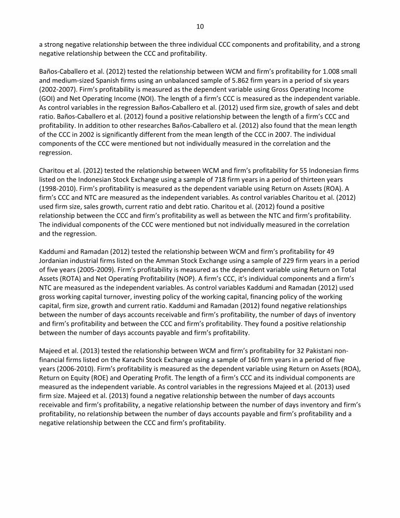
10

a strong negative relationship between the three individual CCC components and profitability, and a strong

negative relationship between the CCC and profitability.

Baños-Caballero et al. (2012) tested the relationship between WCM and firm’s profitability for 1.008 small

and medium-sized Spanish firms using an unbalanced sample of 5.862 firm years in a period of six years

(2002-2007). Firm’s profitability is measured as the dependent variable using Gross Operating Income

(GOI) and Net Operating Income (NOI). The length of a firm’s CCC is measured as the independent variable.

As control variables in the regression Baños-Caballero et al. (2012) used firm size, growth of sales and debt

ratio. Baños-Caballero et al. (2012) found a positive relationship between the length of a firm’s CCC and

profitability. In addition to other researches Baños-Caballero et al. (2012) also found that the mean length

of the CCC in 2002 is significantly different from the mean length of the CCC in 2007. The individual

components of the CCC were mentioned but not individually measured in the correlation and the

regression.

Charitou et al. (2012) tested the relationship between WCM and firm’s profitability for 55 Indonesian firms

listed on the Indonesian Stock Exchange using a sample of 718 firm years in a period of thirteen years

(1998-2010). Firm’s profitability is measured as the dependent variable using Return on Assets (ROA). A

firm’s CCC and NTC are measured as the independent variables. As control variables Charitou et al. (2012)

used firm size, sales growth, current ratio and debt ratio. Charitou et al. (2012) found a positive

relationship between the CCC and firm’s profitability as well as between the NTC and firm’s profitability.

The individual components of the CCC were mentioned but not individually measured in the correlation

and the regression.

Kaddumi and Ramadan (2012) tested the relationship between WCM and firm’s profitability for 49

Jordanian industrial firms listed on the Amman Stock Exchange using a sample of 229 firm years in a period

of five years (2005-2009). Firm’s profitability is measured as the dependent variable using Return on Total

Assets (ROTA) and Net Operating Profitability (NOP). A firm’s CCC, it’s individual components and a firm’s

NTC are measured as the independent variables. As control variables Kaddumi and Ramadan (2012) used

gross working capital turnover, investing policy of the working capital, financing policy of the working

capital, firm size, growth and current ratio. Kaddumi and Ramadan (2012) found negative relationships

between the number of days accounts receivable and firm’s profitability, the number of days of inventory

and firm’s profitability and between the CCC and firm’s profitability. They found a positive relationship

between the number of days accounts payable and firm’s profitability.

Majeed et al. (2013) tested the relationship between WCM and firm’s profitability for 32 Pakistani non-

financial firms listed on the Karachi Stock Exchange using a sample of 160 firm years in a period of five

years (2006-2010). Firm’s profitability is measured as the dependent variable using Return on Assets (ROA),

Return on Equity (ROE) and Operating Profit. The length of a firm’s CCC and its individual components are

measured as the independent variable. As control variables in the regressions Majeed et al. (2013) used

firm size. Majeed et al. (2013) found a negative relationship between the number of days accounts

receivable and firm’s profitability, a negative relationship between the number of days inventory and firm’s

profitability, no relationship between the number of days accounts payable and firm’s profitability and a

negative relationship between the CCC and firm’s profitability.

11

Underneath a scheme with the outcomes of the researches.

Author(s):

Relationship between the

number of days accounts

receivable and Profitability


number of days inventory

and Profitability


number of days accounts

payable and Profitability


Cash Conversion Cycle and

Profitability

Jose et al. (1996) Not individually measured Not individually measured Not individually measured Negative

Shin and Soenen (1998) Not individually measured Not individually measured Not individually measured Negative

Deloof (2003) Negative Negative Negative Negative

Eljelly (2004) Not individually measured Not individually measured Not individually measured Negative

Lazaridis and Tryfonidis (2006) Negative Negative Negative Negative

Padachi (2006) Negative Negative Negative Negative

García-Teruel and Martínez-Solano (2007) Negative Negative Negative Negative

Raheman and Nasr (2007) Negative Negative Negative Negative

Uyar (2009) Not individually measured Not individually measured Not individually measured Negative(a)

Gill et al. (2010) Negative No significant relationship No significant relationship Positive

Mathuva (2010) Negative Positive Positive Negative

Afeef (2011) Negative(b) Negative(b) No significant relationship No significant relationship

Alipour (2011) Negative Negative Positive Negative

Ching et al. (2011) Not individually measured Negative Not individually measured Positive

Sharma and Kumar (2011) Positive Negative Negative Positive

Ashraf (2012) Negative Negative Negative Negative

Baños-Caballero et al. (2012) Not individually measured Not individually measured Not individually measured Positive

Charitou et al. (2012) Not individually measured Not individually measured Not individually measured Positive

Kaddumi and Ramadan (2012) Negative Negative Positive Negative

Majeed et al. (2013) Negative Negative No significant relationship Negative

Notes:

(a): Uyar (2009) only performed a correlation analysis to test the relationship. (b): Afeef (2011) found a negative relationship through the Operating Profit to Sales ratio and no significant relationship through Return on Assets.

Table 3: Overview of found relationships by different authors

12

A notable difference between the articles is their choice how to measure the dependent variable;

profitability. We have seen GOI which is nearly equivalent to GOP (Shin and Soenen, 1998; Deloof, 2003;

Lazaridis and Tryfonidis, 2006; Gill et al., 2010; Alipour, 2011; Baños-Caballero et al., 2012), NOP which is

nearly equivalent to NOI (Shin and Soenen, 1998; Deloof, 2003; Eljelly, 2004; Raheman and Nasr, 2007;

Mathuva, 2010; Ashraf, 2012; Baños-Caballero et al., 2012; Kaddumi and Ramadan, 2012), EBIT (Majeed et

al., 2013), OPS (Afeef, 2011), ROA (Jose et al., 1996; García-Teruel and Martínez-Solano, 2007; Uyar, 2009;

Afeef, 2011; Ching et al., 2011; Sharma and Kumar, 2011; Charitou et al., 2012; Majeed et al., 2013), ROE

(Jose et al., 1996; Uyar, 2009; Ching et al., 2011; Majeed et al., 2013), ROS (Ching et al., 2011) and ROTA

(Padachi, 2006; Kaddumi and Ramadan, 2012). The calculations of these variables can be found in table 4

below.

Measurement methods: Calculations:

Gross Operating Income (GOI) &

Gross Operating Profit (GOP) ==== #�� − �� *�� #��

1�� − 4��

Net Operating Profitability (NOP) &

Net Operating Income (NOI) ====

5�� )�� + ��1�� − 4��

Operating Profit (EBIT) ==== 6�� 7�� )�� 1�8

Operating Profit to Sales (OPS) ==== 5�� +��

"�� #��

Return on Assets (ROA) ==== "�� )��

�!�� 1��

Return on Equity (ROE) ==== "�� )��

69��

Return on Sales (ROS) ==== "�� )��

#��

Return on Total Assets (ROTA) ==== 6�� 7�� )�� 1�8�� (67)1)

1��

Table 4: Dependent variables and their calculations

For the GOI, GOP, NOP and NOI, some authors decide to divide with all total assets (Baños-Caballero et al.,

2012), others decide to divide with total assets and deduct financial assets (Deloof, 2003; Lazaridis and

Tryfonidis, 2006; Raheman and Nasr, 2007; Gill et al., 2010; Mathuva, 2010; Alipour, 2011; Ashraf, 2012)

and even others decide to divide with net sales (Shin and Soenen, 1998; Eljelly, 2004).

The independent variables are the same in most studies, except for Shin and Soenen (1998) who chose for

the NTC, Eljelly (2004) which chose for the CG and Ching et al. (2011) who chose for DWC. All other authors

chose for the CCC and its individual components; the number of days accounts receivable, the number of

days inventory and the number of days accounts payable or chose for a combination of both, the CCC and

the NTC. The NTC, CG and DWC are comparable with the CCC. The calculations of the independent

variables CCC and NTC can be found in paragraph 2.2 the cash conversion cycle. The calculations for the CG

and DWC are equal to the calculation of the CCC.

13

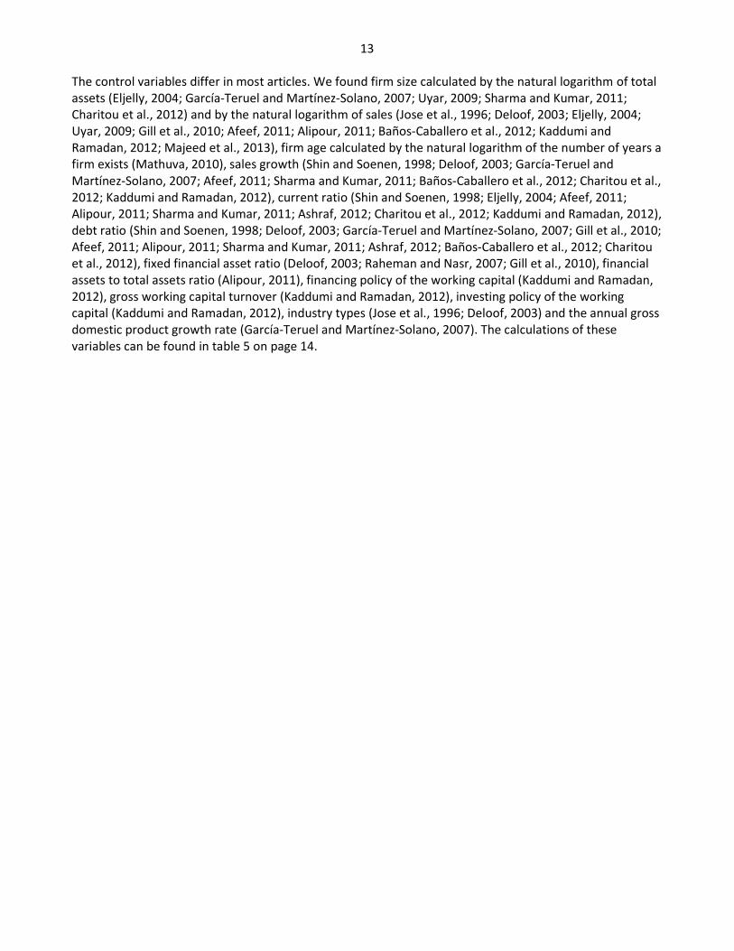
The control variables differ in most articles. We found firm size calculated by the natural logarithm of total

assets (Eljelly, 2004; García-Teruel and Martínez-Solano, 2007; Uyar, 2009; Sharma and Kumar, 2011;

Charitou et al., 2012) and by the natural logarithm of sales (Jose et al., 1996; Deloof, 2003; Eljelly, 2004;

Uyar, 2009; Gill et al., 2010; Afeef, 2011; Alipour, 2011; Baños-Caballero et al., 2012; Kaddumi and

Ramadan, 2012; Majeed et al., 2013), firm age calculated by the natural logarithm of the number of years a

firm exists (Mathuva, 2010), sales growth (Shin and Soenen, 1998; Deloof, 2003; García-Teruel and

Martínez-Solano, 2007; Afeef, 2011; Sharma and Kumar, 2011; Baños-Caballero et al., 2012; Charitou et al.,

2012; Kaddumi and Ramadan, 2012), current ratio (Shin and Soenen, 1998; Eljelly, 2004; Afeef, 2011;

Alipour, 2011; Sharma and Kumar, 2011; Ashraf, 2012; Charitou et al., 2012; Kaddumi and Ramadan, 2012),

debt ratio (Shin and Soenen, 1998; Deloof, 2003; García-Teruel and Martínez-Solano, 2007; Gill et al., 2010;

Afeef, 2011; Alipour, 2011; Sharma and Kumar, 2011; Ashraf, 2012; Baños-Caballero et al., 2012; Charitou

et al., 2012), fixed financial asset ratio (Deloof, 2003; Raheman and Nasr, 2007; Gill et al., 2010), financial

assets to total assets ratio (Alipour, 2011), financing policy of the working capital (Kaddumi and Ramadan,

2012), gross working capital turnover (Kaddumi and Ramadan, 2012), investing policy of the working

capital (Kaddumi and Ramadan, 2012), industry types (Jose et al., 1996; Deloof, 2003) and the annual gross

domestic product growth rate (García-Teruel and Martínez-Solano, 2007). The calculations of these

variables can be found in table 5 on page 14.

14

Measurement methods: Calculations:

Firm Size ====

-�(1�� )

or -�(1�� #��)

Firm Age ==== -�("�� 8��)

Sales Growth ==== ("�� #�� − "�� #��:;)

"�� #��:;

Current Ratio ==== ��

�� -��

Debt Ratio ==== 1�� -��

1��

Fixed Financial Asset ratio ==== 48�� 4��

1��

Financial Assets to Total Assets ratio ==== 4��

1��

Financing Policy of the Working Capital ==== �� -��

1��

Gross Working Capital Turnover ==== "�� #��

��

Investing Policy of the Working Capital ==== ��

1��

Industry types ==== )��

Annual GDP growth rate ==== (*�+� − *�+�:;)

*�+�:;

Notes:

�: time in years.

Table 5: Control variables and their calculations

15

3. Hypotheses The aim of this research is to examine the relationship between WCM and firm profitability. To prove the

relationship between WCM and firm profitability, this research will use a hypothesis testing approach.

Therefor this research contains five testable hypotheses. As noticed in the prior research it seems plausible

that there is a negative relationship between the WCM and the profitability of firms.

According to this information the following problem statement can be formulated:

“�� ? ”

This problem statement will be analysed during this research and hopefully contribute to the existing

knowledge on WCM, which is known to be an important aspect of Financial Management.

The objectives of this research are:

� To find a relationship between firm profitability and the number of days accounts receivable over a

period of nine years for 67 Dutch listed firms, and

� To find a relationship between firm profitability and the number of days inventory over a period of nine

years for 67 Dutch listed firms, and

� To find a relationship between firm profitability and the number of days accounts payable over a

period of nine years for 67 Dutch listed firms, and

� To find a relationship between firm profitability and the Cash Conversion Cycle over a period of nine

years for 67 Dutch listed firms, and

� To find a relationship between firm profitability and the Net Trade Cycle over a period of nine years for

67 Dutch listed firms, and

� To find the effects of firm size, sales growth, current ratio, debt ratio and the annual GDP growth rate

on firm profitability over a period of nine years for 67 Dutch listed firms.

The relationships as mentioned above are considered to be of high importance to test the relationship

between WCM and firm profitability, while WCM refers to the management of working capital which is the

sum of current assets minus current liabilities. The current assets are accounts receivable and inventory,

and the current liabilities are accounts payable.

As noticed in the prior research it seems plausible that there exists a negative relationship between the

number of days accounts receivable and the profitability of firms (Deloof, 2003; Lazaridis and Tryfonidis,

2006; Padachi, 2006; García-Teruel and Martínez-Solano, 2007; Raheman and Nasr, 2007; Gill et al., 2010;

Mathuva, 2010; Afeef, 2011; Alipour, 2011; Ashraf, 2012; Kaddumi and Ramadan, 2012; Majeed et al.,

2013), except for Sharma and Kumar (2011) who found a positive relationship between the number of days

accounts receivable and the profitability of firms. Following the majority of the reviewed literature, a

negative relationship in the obtained dataset seems plausible as well.

In this research, the following hypothesis is drawn:

<�� ;: 1�� !� �� >�� !�� .

This hypothesis implies that if the number of days accounts receivable decrease, the profitability of Dutch

listed firms increase. Vice versa, if the number of days accounts receivable increase, the profitability of

Dutch listed firms decrease.


number of days inventory and the profitability of firms (Deloof, 2003; Lazaridis and Tryfonidis, 2006;

16

Padachi, 2006; García-Teruel and Martínez-Solano, 2007; Raheman and Nasr, 2007; Afeef, 2011; Alipour,

2011; Ching et al., 2011; Sharma and Kumar, 2011; Ashraf, 2012; Kaddumi and Ramadan, 2012; Majeed et

al., 2013), except for Mathuva (2010) who found a positive relationship and Gill et al. (2010) who found no

significant relationship between the number of days inventory and the profitability of firms. Following the

majority of the reviewed literature, a negative relationship in the obtained dataset seems plausible as well.


<�� @: 1�� !� �� >�� !�� .

This hypothesis implies that if the number of days inventory decrease, the profitability of Dutch listed firms

increase. Vice versa, if the number of days inventory increase, the profitability of Dutch listed firms

decrease.


number of days accounts payable and the profitability of firms (Deloof, 2003; Lazaridis and Tryfonidis,

2006; Padachi, 2006; García-Teruel and Martínez-Solano, 2007; Raheman and Nasr, 2007; Sharma and

Kumar, 2011; Ashraf, 2012), conversely some authors found a positive relationship (Mathuva, 2010;

Alipour, 2011; Kaddumi and Ramadan, 2012) or no significant relationship (Gill et al., 2010; Afeef, 2011;

Majeed et al., 2013) between the number of days accounts payable and the profitability of firms. Following

the majority of the reviewed literature, a negative relationship in the obtained dataset seems plausible as

well.


<�� &: 1�� !� �� >�� .

This hypothesis implies that if the number of days accounts payable decrease, the profitability of Dutch

listed firms decrease. Vice versa, if the number of days accounts payable increase, the profitability of Dutch

listed firms increase.


length of the CCC and the profitability of firms (Jose et al., 1996; Deloof, 2003; Eljelly, 2004; Lazaridis and

Tryfonidis, 2006; Padachi, 2006; García-Teruel and Martínez-Solano, 2007; Raheman and Nasr, 2007; Uyar,

2009; Mathuva, 2010; Alipour, 2011; Ashraf, 2012; Kaddumi and Ramadan, 2012; Majeed et al., 2013),

conversely some authors found a positive relationship (Gill et al., 2010; Ching et al., 2011; Sharma and

Kumar, 2011; Baños-Caballero et al., 2012; Charitou et al., 2012) or no significant relationship (Afeef, 2011)

between the length of the CCC and the profitability of firms. Following the majority of the reviewed

literature, a negative relationship in the obtained dataset seems plausible as well.


<�� A: 1�� !� �� >�� !�� .

This hypothesis implies that if the CCC period decreases, the profitability of Dutch listed firms increase.

Vice versa, if the CCC period increases, the profitability of Dutch listed firms decrease.

17


length of the NTC and the profitability of firms (Shin and Soenen, 1998; Kaddumi and Ramadan, 2012),

conversely some authors found a positive relationship between the length of the NTC and the profitability

of firms (Ching et al., 2011; Charitou et al., 2012). Because the number of studies reporting a positive or

negative relationship are equally shared, there is no majority to follow. The NTC is comparable with the

CCC, and most of the studies about the relationship between the CCC and the profitability of firms report a

negative relationship. Following the majority of the reviewed literature for both the NTC and CCC, a

negative relationship in the obtained dataset seems plausible between the length of the NTC and the

profitability of firms as well.


<�� (: 1�� !� �� >�� .

This hypothesis implies that if the NTC period decreases, the profitability of Dutch listed firms increase.

Vice versa, if the NTC period increases, the profitability of Dutch listed firms decrease.

18

4. Methodology This research uses statistics as a tool to accept or reject the hypotheses as discussed in the previous

chapter. The dependent, independent and control variables used in the descriptive statistics, the

correlation analysis and the regression models are explained in paragraph 4.1. The regression models, as

linked to the different hypotheses can be found in paragraph 4.2. A brief explanation of the collected data

can be found in paragraph 4.3.

4.1 Variables In this paragraph the dependent, independent and control variables for this research will be indicated. The

choice of the variables for this research is affected by the prior research on the relationship between WCM

and firm profitability as discussed in the literature review in chapter two. Prior research did not always

mention why a specific variable is used, but the choice is sometimes limited due to the unavailability of

data. The names for the data in the variables below differ from the names for the data in the literature

review, because the names for the data in the variables are equal to the names provided through the

ORBIS database. The use different names for the variables do not change the outcome of the calculations.

In this research the independent variable for WCM is the cause, the dependent variable for firm

profitability the effect. In other words, WCM policies cause an effect on firm profitability. The control

variables in this research attempt to explain the relationship between the dependent and independent

variables.

4.1.1 Dependent variables The dependent variables in this research measure firm profitability. In the reviewed literature, eight

different variables are used to measure firm profitability. The majority of the reviewed literature chose for

Return on Assets (ROA) or Gross Operating Profit (GOP). Other chosen variables are: Net Operating Profit

(NOP), Earnings before Interest and Taxes (EBIT), Operating Profit to Sales (OPS), Return on Equity (ROE),

Return on Sales (ROS) and Return on Total Assets (ROTA). The most simple and commonly used variable for

measuring firm profitability is ROA. The difference between ROA and ROTA is that ROA is based on income

after interest and taxes (net income), and ROTA is based on income before interest and taxes. ROA is a

good measure for firm profitability since it relates the firm profitability to a firms asset base (Padachi,

2006; Leach and Melicher, 2011; Sharma and Kumar, 2011), and is used by various authors (Jose et al.,

1996; García-Teruel and Martínez-Solano, 2007; Uyar, 2009; Afeef, 2011; Ching et al., 2011; Sharma and

Kumar, 2011; Charitou et al., 2012; Majeed et al., 2013). ROA is measured by dividing net income with

average total assets.

�� (�5�) = "�� )�� 1��

For some of the firms in the dataset, financial assets cover a significant part of the firms total assets.

Financial assets are long term receivables, long term investments in other firms, investments in properties,

other investments and/or other long term assets (see: balance sheet in appendix A2). Firms where financial

assets cover a significant part of the firms total assets, the firms operating activities will have little

influence on the return on (total) assets. ROA does not exclude financial assets, and for that reason this

research has chosen to add a second dependent variable which does exclude financial assets from the

profitability measure, namely GOP.

GOP is a good measure for firm profitability since it relates the firm profitability to a firms asset base minus

the financial assets (Deloof, 2003), and is used by various authors (Shin and Soenen, 1998; Deloof, 2003;

Lazaridis and Tryfonidis, 2006; Gill et al., 2010; Alipour, 2011; Baños-Caballero et al., 2012).

19

GOP is calculated by dividing sales minus cash costs of goods sold with total assets minus financial assets.

The calculation followed the majority of the authors.

*�� 5�� +�� (*5+) = #�� − �� *�� #��1�� − 4��

Both ROA and GOP will be used as a measurement for firm profitability in this research. By choosing two

variables the research can be more easily compared with other researches to strengthen the results.

4.1.2 Independent variables As mentioned in the literature review, WCM consists out of three individual components which together

form the CCC, namely: the number of days accounts receivable, the number of days accounts payable and

the number of days inventory (Deloof, 2003). In this research WCM is measured through the three

individual components of the CCC, the CCC and NTC. Doing so makes this research more comparable with

other researches, while most of the researches chose for CCC or NTC instead of both.

The number of days accounts payable (DAR) variable already exists in ORBIS and can be found as collection

period. The calculation is as follow:

"�� !�� = (�� !�� − �� )

�� !�� (��) = ��"�� #��$ ∗ &'(

The number of days inventory (DI) variable does not exist in ORBIS and is calculated as follow:

"�� #�� )�!�� #�� = ��> �� + �� +�� +4�� *�� + )�!�� +��-+��

�� )�!�� (�)) = "�� #�� )�!�� *�� #�� $ ∗ &'(

This calculation for the number of days accounts payable differs from the calculation found in the

paragraph 2.2 the cash conversion cycle, while in this research average accrued liabilities are not added to

the average accounts payable. All the reviewed literature has not mentioned accrued liabilities, accrued

liabilities are not direct payables for firms and the data cannot be individually obtained from the ORBIS

database. For these reasons accrued liabilities are excluded for the rest of the research. In the ORBIS

database payables are described as creditors and/or trade creditors. The number of days accounts payable

(DAP) variable already exists in ORBIS and can be found as credit period. The calculation is as follow:

�� +�� (��+) = �� *�� #��$ ∗ &'(

The cash conversion cycle period (CCC) variable does not exist in ORBIS and is calculated as follow:

�� !�� ( ) = (�� + �)) − ��+

The net trade cycle period (NTC) variable does not exist in ORBIS and is calculated as follow:

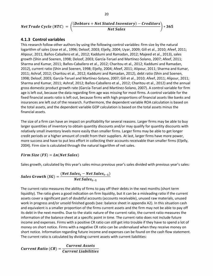
20

"�� 1�� ("1 ) = 2(�� + "�� #�� )�!��) − ��"�� #�� 3 ∗ &'(

4.1.3 Control variables This research follow other authors by using the following control variables: firm size by the natural

logarithm of sales (Jose et al., 1996; Deloof, 2003; Eljelly, 2004; Uyar, 2009; Gill et al., 2010; Afeef, 2011;

Alipour, 2011; Baños-Caballero et al., 2012; Kaddumi and Ramadan, 2012; Majeed et al., 2013), sales

growth (Shin and Soenen, 1998; Deloof, 2003; García-Teruel and Martínez-Solano, 2007; Afeef, 2011;

Sharma and Kumar, 2011; Baños-Caballero et al., 2012; Charitou et al., 2012; Kaddumi and Ramadan,

2012), current ratio (Shin and Soenen, 1998; Eljelly, 2004; Afeef, 2011; Alipour, 2011; Sharma and Kumar,

2011; Ashraf, 2012; Charitou et al., 2012; Kaddumi and Ramadan, 2012), debt ratio (Shin and Soenen,

1998; Deloof, 2003; García-Teruel and Martínez-Solano, 2007; Gill et al., 2010; Afeef, 2011; Alipour, 2011;

Sharma and Kumar, 2011; Ashraf, 2012; Baños-Caballero et al., 2012; Charitou et al., 2012) and the annual

gross domestic product growth rate (García-Teruel and Martínez-Solano, 2007). A control variable for firm

age is left out, because the data regarding firm age was missing for most firms. A control variable for the

fixed financial assets ratio is left out, because firms with high proportions of financial assets like banks and

insurances are left out of the research. Furthermore, the dependent variable ROA calculation is based on

the total assets, and the dependent variable GOP calculation is based on the total assets minus the

financial assets.

The size of a firm can have an impact on profitability for several reasons. Larger firms may be able to buy

larger quantities of inventory to obtain quantity discounts and/or may qualify for quantity discounts with

relatively small inventory levels more easily than smaller firms. Larger firms may be able to get longer

credit periods or a higher amount of credit from their suppliers. At last, larger firms have more power,

more success and have to put less effort in collecting their accounts receivable than smaller firms (Eljelly,

2004). Firm size is calculated through the natural logarithm of net sales.

4�� #C� (4#) = -�("�� #��)

Sales growth, calculated by this year’s sales minus previous year’s sales divided with previous year’s sales:

#�� *��>�� (#*) = ("�� #�� − "�� #��:;)"�� #��:;

The current ratio measures the ability of firms to pay off their debts in the next months (short term

liquidity). The ratio gives a good indication on firm liquidity, but it can be a misleading ratio if the current

assets cover a significant part of doubtful accounts (accounts receivable), unused raw materials, unused

work in progress and/or unsold finished goods (see: balance sheet in appendix A2). In this situation cash

and equivalent is a smaller proportion of the firms current assets and the firm may not be able to pay off

its debt in the next months. Due to the static nature of the current ratio, the current ratio measures the

information of the balance sheet at a specific point in time. The current ratio does not include future

income and expenses. Firms with a positive CR ratio can still get into trouble if they have to spend a lot of

money on short notice. Firms with a negative CR ratio can be undervalued when they receive money on

short notice. Information regarding future income and expenses can be found on the cash flow statement.

The current ratio is calculated by dividing current assets with current liabilities:

�� ( �) = �� -��

21

The debt ratio measures the leverage of firms. The ratio gives a good indication on the amount of a firms

total assets that is financed through external debt. The debt ratio is calculated by dividing total liabilities

with total assets:

�� (��) = 1�� -��1��

The annual GDP growth rate shows the economic condition of the country the firms in the dataset operate

in (in this dataset: the Netherlands). The annual GDP is calculated as follow;

*�+� = �� + �� !�� + ��!�� + (�8�� − ��)

, and the annual GDP growth rate is calculated as follow:

�� *�+ *��>�� (*�+*) = (*�+� − *�+�:;)*�+�:;

22

4.2 Research design The two dependent variables, five independent variables and five control variables will be tested through a

Pearson correlation, a pooled Ordinary Least Squares regression model (OLS) and through a Fixed-Effects

regression model (FEM) or Generalized Least Squares Random-Effects regression model (REM).

Underneath a scheme with the different regressions chosen by other authors.

Author(s): OLS regression FEM regression REM regression

Jose et al. (1996)(a)

Shin and Soenen (1998)(b) �

Deloof (2003) � �

Eljelly (2004)(c) �

Lazaridis and Tryfonidis (2006) �

Padachi (2006) � � �

García-Teruel and Martínez-Solano (2007) � � �

Raheman and Nasr (2007) � �

Uyar (2009)(d)

Gill et al. (2010)(e) � �

Mathuva (2010) � �

Afeef (2011) �

Alipour (2011)(f) �

Ching et al. (2011) �

Sharma and Kumar (2011) �

Ashraf (2012)(g) �

Baños-Caballero et al. (2012) �

Charitou et al. (2012) �

Kaddumi and Ramadan (2012) � �

Majeed et al. (2013) � (a): Jose et al. (1996) tested the relationship with a univariate regression analysis. (b): Shin and Soenen (1998) also performed cross-section regressions. (c): Eljelly (2004) also performed a sector regression and a temporal regression. (d): Uyar (2009) only tested the relationship with a correlation analysis. (e): Gill et al. (2010) also performed a Weighted Least Squares regression analysis. (f): Alipour (2011) also performed a Weighted Least Squares regression analysis. (g): Ashraf (2012) also performed a panel data regression.

Table 6: Overview of used regression models by different authors

The OLS regression model is a linear regression applied to the entire dataset, explaining the variations of

profitability between firms. The OLS regression models are tested for multicollinearity through the

Variance Inflation Factor (VIF) in STATA8. Multicollinearity can appear in a multiple regression model and

appears when two or more independent variables are highly correlated. Multicollinearity can occur when

the regression model covers too many variables and when some of the different variables measure the

same phenomena. If multicollinearity is present, small changes in the regression model or the dataset may

change the coefficient estimates for the independent variables, and the individual effects of each

independent variable on the dependent variable are probably invalid. The VIF is defined as;

D)4 = ;E; − � @FG

8 Command STATA: estat vif

23

, where � @F is the multiple correlation of the independent variable HF with the other independent

variables. Multicollinearity is problematic when VIF values exceed 10, if the values exceed 10 the

coefficients for the regression analysis are probably poorly estimated.

The OLS regression models are tested for heteroskedasticity with the White’s test in STATA9. The null

hypothesis assumes homoskedasticity and the alternative hypothesis assumes heteroskedasticity.

If the p-value is below 0.05 (5%) we have no argument to accept the null hypothesis and accept the

alternative hypothesis. Heteroskedasticity exists when the variances of the error terms are different for all

observations, meaning that dependent variable H and random error � are heteroskedastic.

The problem of heteroskedasticity can be corrected by using robust standard error in the OLS regression.

The coefficient estimates for the independent variables stay the same, but the p-values are more accurate

due to the changed standard errors.

To test the dataset with a FEM regression or REM regression, the dataset has to be declared as a panel

data set in STATA10. As the data panel ID variable is chosen for the firm number and as the time variable is

chosen for the year. Panel data observes multiple cases (people, industries, firms, countries, etc.) at

different periods in time. Other names for panel data are cross-sectional time series data and longitudinal

data. The FEM regression and REM regression consider single cases (in this case firms) across time periods

(in this case nine years), explaining the variations of profitability within firms. This panel dataset observes

67 firms in a period of nine years. With 603 firm observations this can be identified as a strongly balanced

panel dataset.

To test whether the FEM regression or the REM regression is the appropriate regression model, a Hausman

test is performed. Within the Hausman test the null hypothesis indicates that the REM regression is the

appropriate regression method, and the alternative hypothesis indicates that the FEM regression is the

appropriate regression method. This means that if the P-value equal to 0.05 (5%) or less, we reject the null

hypothesis and accept the alternative hypothesis.

To test whether the REM regression or the OLS regression is the appropriate regression model, a Breusch

and Pagan Lagrangian multiplier test is performed in STATA11. Within the Breusch and Pagan Lagrangian

multiplier test the null hypothesis indicates that the OLS regression is the appropriate regression method,

and the alternative hypothesis indicates that the REM regression is the appropriate regression method.

This means that if the P-value equal to 0.05 (5%) or less, we reject the null hypothesis and accept the

alternative hypothesis.

General model used in the analysis:

+�� = �(�� , 4�� )

These two regression models are used to test the first hypothesis of this research, and will test the

relationship between the number of days accounts receivable and the profitability of Dutch listed firms:

Regression equation 1: �5�� = J + K;(��) + K@( ��) + K&(��) + KA(4#�) + K((#*�) + K'(*�+*�) + L + M� + N�

Regression equation 2: *5+� = J + K;(��) + K@( ��) + K&(��) + KA(4#�) + K((#*�) + K'(*�+*�) + L + M� + N� 9 Command STATA: imtest, white 10 Command STATA: xtset Companyno Year, yearly 11 Command STATA: xttest0

24

These two models are used to test the second hypothesis of this research, and will test the relationship

between the number of days inventory and the profitability of Dutch listed firms:

Regression equation 3: �5�� = J + K;(�)�) + K@( ��) + K&(��) + KA(4#�) + K((#*�) + K'(*�+*�) + L + M� + N�

Regression equation 4: *5+� = J + K;(�)�) + K@( ��) + K&(��) + KA(4#�) + K((#*�) + K'(*�+*�) + L + M� + N�

These two models are used to test the third hypothesis of this research, and will test the relationship

between the number of days accounts payable and the profitability of Dutch listed firms:

Regression equation 5: �5�� = J + K;(��+�) + K@( ��) + K&(��) + KA(4#�) + K((#*�) + K'(*�+*�) + L + M� + N�

Regression equation 6: *5+� = J + K;(��+�) + K@( ��) + K&(��) + KA(4#�) + K((#*�) + K'(*�+*�) + L + M� + N�

These two models are used to test the fourth hypothesis of this research, and will test the relationship

between the cash conversion cycle period and the profitability of Dutch listed firms:

Regression equation 7: �5�� = J + K;( �) + K@( ��) + K&(��) + KA(4#�) + K((#*�) + K'(*�+*�) + L + M� + N�

Regression equation 8: *5+� = J + K;( �) + K@( ��) + K&(��) + KA(4#�) + K((#*�) + K'(*�+*�) + L + M� + N�

These two models are used to test the fourth hypothesis of this research, and will test the relationship

between the net trade cycle period and the profitability of Dutch listed firms:

Regression equation 9: �5�� = J + K;("1 �) + K@( ��) + K&(��) + KA(4#�) + K((#*�) + K'(*�+*�) + L + M� + N�

Regression equation 10: *5+� = J + K;("1 �) + K@( ��) + K&(��) + KA(4#�) + K((#*�) + K'(*�+*�) + L + M� + N� �5�� and *5+� as a measurement for firm profitability, J as the constant, �� as the number of days

accounts receivable, �)� as the number of days inventory, ��+� as the number of days accounts

payable, � as the cash conversion cycle period, "1 � as the net trade cycle period, �� as the firm

liquidity measured by the current ratio, �� as the firm leverage measured by the debt ratio, 4#� as the

firm size measured by the natural logarithm of sales, #*� as the annual firm sales growth, *�+*� as the

annual growth of the gross domestic product, L as the unobservable heterogeneity, measuring the

particular firm characteristics, M� as the time dummy for firm year controls, N� as the residual errors, as a

firm ranging from 1 to 67, � as time in years ranging from 2004 to 2012.

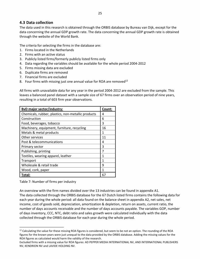
25

4.3 Data collection The data used in this research is obtained through the ORBIS database by Bureau van Dijk, except for the

data concerning the annual GDP growth rate. The data concerning the annual GDP growth rate is obtained

through the website of the World Bank.

The criteria for selecting the firms in the database are:

1. Firms located in the Netherlands

2. Firms with an active status

3. Publicly listed firms/formerly publicly listed firms only

4. Data regarding the variables should be available for the whole period 2004-2012

5. Firms missing data are excluded

6. Duplicate firms are removed

7. Financial firms are excluded

8. Four firms with missing just one annual value for ROA are removed12

All firms with unavailable data for any year in the period 2004-2012 are excluded from the sample. This

leaves a balanced panel dataset with a sample size of 67 firms over an observation period of nine years,

resulting in a total of 603 firm year observations.

BvD major sector/industry: Count:

Chemicals, rubber, plastics, non-metallic products 4

Construction 6

Food, beverages, tobacco 3

Machinery, equipment, furniture, recycling 16

Metals & metal products 1

Other services 11

Post & telecommunications 4

Primary sector 3

Publishing, printing 7

Textiles, wearing apparel, leather 1

Transport 1

Wholesale & retail trade 9

Wood, cork, paper 1

Total: 67

Table 7: Number of firms per industry

An overview with the firm names divided over the 13 industries can be found in appendix A1.

The data collected through the ORBIS database for the 67 Dutch listed firms contains the following data for

each year during the whole period: all data found on the balance sheet in appendix A2, net sales, net

income, cost of goods sold, depreciation, amortization & depletion, return on assets, current ratio, the

number of days accounts receivable and the number of days accounts payable. The variables GOP, number

of days inventory, CCC, NTC, debt ratio and sales growth were calculated individually with the data

collected through the ORBIS database for each year during the whole period.

12 Calculating the value for these missing ROA figures is considered, but seem to be not an option. The rounding of the ROA

figures for the known years were just unequal to the data provided by the ORBIS database. Adding the missing values for the

ROA figures as calculated would harm the validity of the research.

Excluded firms with a missing value for ROA figures: AD PEPPER MEDIA INTERNATIONAL NV, AND INTERNATIONAL PUBLISHERS

NV, KENDRION NV and LAVIDE HOLDING NV.

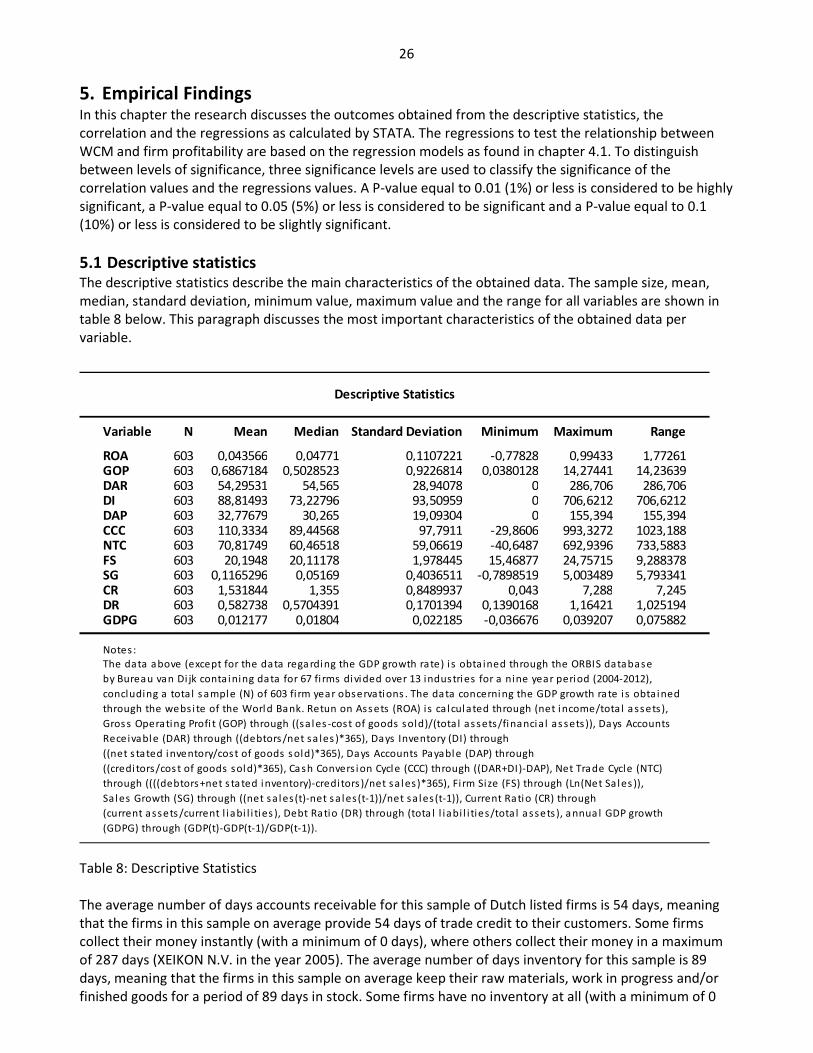
26

5. Empirical Findings In this chapter the research discusses the outcomes obtained from the descriptive statistics, the

correlation and the regressions as calculated by STATA. The regressions to test the relationship between

WCM and firm profitability are based on the regression models as found in chapter 4.1. To distinguish

between levels of significance, three significance levels are used to classify the significance of the

correlation values and the regressions values. A P-value equal to 0.01 (1%) or less is considered to be highly

significant, a P-value equal to 0.05 (5%) or less is considered to be significant and a P-value equal to 0.1

(10%) or less is considered to be slightly significant.

5.1 Descriptive statistics The descriptive statistics describe the main characteristics of the obtained data. The sample size, mean,

median, standard deviation, minimum value, maximum value and the range for all variables are shown in

table 8 below. This paragraph discusses the most important characteristics of the obtained data per

variable.

Variable N Mean Median Standard Deviation Minimum Maximum Range

ROA 603 0,043566 0,04771 0,1107221 -0,77828 0,99433 1,77261GOP 603 0,6867184 0,5028523 0,9226814 0,0380128 14,27441 14,23639DAR 603 54,29531 54,565 28,94078 0 286,706 286,706DI 603 88,81493 73,22796 93,50959 0 706,6212 706,6212DAP 603 32,77679 30,265 19,09304 0 155,394 155,394CCC 603 110,3334 89,44568 97,7911 -29,8606 993,3272 1023,188NTC 603 70,81749 60,46518 59,06619 -40,6487 692,9396 733,5883FS 603 20,1948 20,11178 1,978445 15,46877 24,75715 9,288378SG 603 0,1165296 0,05169 0,4036511 -0,7898519 5,003489 5,793341CR 603 1,531844 1,355 0,8489937 0,043 7,288 7,245DR 603 0,582738 0,5704391 0,1701394 0,1390168 1,16421 1,025194GDPG 603 0,012177 0,01804 0,022185 -0,036676 0,039207 0,075882

Notes:

(GDPG) through (GDP(t)-GDP(t-1)/GDP(t-1)).

Receivable (DAR) through ((debtors /net sa les )*365), Days Inventory (DI) through

((net s tated inventory/cost of goods s old)*365), Days Accounts Payable (DAP) through

((credi tors/cos t of goods sold)*365), Ca sh Convers i on Cycle (CCC) through ((DAR+DI)-DAP), Net Trade Cycle (NTC)

through ((((debtors+net s ta ted inventory)-creditors )/net sa les)*365), Firm Size (FS) through (Ln(Net Sa les )),

Sa les Growth (SG) through ((net sa les(t)-net s a les(t-1))/net sa les(t-1)), Current Ratio (CR) through

(current assets /current l i abi l i ties ), Debt Ratio (DR) through (tota l l iabi l i ties/tota l a ssets), a nnua l GDP growth

Descriptive Statistics

The data above (except for the data rega rding the GDP growth rate) i s obta ined through the ORBIS database

by Bureau van Di jk containing data for 67 fi rms divided over 13 industries for a nine year period (2004-2012),

concluding a tota l s ample (N) of 603 fi rm year observations . The data concerning the GDP growth ra te i s obta ined

through the webs i te of the World Bank. Retun on Assets (ROA) is ca lculated through (net income/tota l a ssets),

Gros s Operating Profi t (GOP) through ((sa les -cost of goods sold)/(tota l as sets/financia l as sets)), Days Accounts

Table 8: Descriptive Statistics

The average number of days accounts receivable for this sample of Dutch listed firms is 54 days, meaning

that the firms in this sample on average provide 54 days of trade credit to their customers. Some firms

collect their money instantly (with a minimum of 0 days), where others collect their money in a maximum

of 287 days (XEIKON N.V. in the year 2005). The average number of days inventory for this sample is 89

days, meaning that the firms in this sample on average keep their raw materials, work in progress and/or

finished goods for a period of 89 days in stock. Some firms have no inventory at all (with a minimum of 0

27

days), where others have inventory for a maximum of 707 days (XEIKON N.V. in the year 2005). The

average number of days accounts payable for this sample is 33 days, meaning that firms in this sample

finance themselves with trade credit provided by their suppliers on an average period of 33 days. Some

firms pay their bills instantly (with a minimum of 0 days), where others postpone their payments to a

maximum of 155 days (KONINKLIJKE BRILL N.V. in the year 2012). This results in an average CCC period of

89 days for this sample, meaning that most of the firms in this sample do not finance themselves with

trade credit provided by their suppliers but provide trade credit to their customers and take the risk of

keeping inventories. Some of the firms collect their accounts receivable before paying their accounts

payable (with a minimum and negative CCC of 30 days for X5 RETAIL GROUP N.V. in the year 2007),

probably these firms have very little to no inventories. Other firms take the risk of keeping inventories for a

long period and providing trade credit to their customers, but not postponing payments towards their

suppliers (with a maximum CCC of 993 days for XEIKON N.V. in the year 2005). The values for the NTC are

comparable with the values for the CCC, having an average NTC period of 71 days (with a minimum and

negative NTC period of 41 days for X5 RETAIL GROUP N.V. in the year 2007 and a maximum NTC period of

693 days for XEIKON N.V. in the year 2005).

The firm size calculated by the natural logarithm of sales has a minimum of 15,46877 corresponding with

the data for CATALIS S.E. in the year 2004 where the firm has €5,224,000 of sales, and a maximum of

24.75715 corresponding with the data for AIRBUS N.V. in the year 2012 where the firm has

€56,480,000,000 of sales. On average the firms in this sample have a natural logarithm of sales of 20.1948

corresponding with a sales of approximately €589,508,679.

The firm sales growth percentage has a minimum of -79% for XEIKON N.V. in the year 2005 where sales

declined from €27,276,000 in 2004 to €5,732,000 in 2005. The sales growth percentage has a maximum of

+500% for XEIKON N.V. in the year 2006 where sales improved from €5,732,000 in 2005 to €34,412,000 in

2006. These extreme values for the sales growth of XEIKON N.V. could be caused by the number of days

accounts receivable, the number of days inventory, the CCC and the NTC of XEIKON N.V. in the year 2005.

On average the firms in this sample improved their sales with 11,65%.

The current ratio has a minimum of 4,3% for NIEUWE STEEN INVESTMENTS N.V. in the year 2008 and a

maximum of 728,8% for HYDRATEC INDUSTRIES N.V. in the year 2008. On average the firms in this sample

have a current ratio of 153,2%, meaning that on average the current assets are 153,2% of the current

liabilities. So it seems the majority of the firms are healthy and able to pay off their debts in the next

months (short term liquidity).

The debt ratio has a minimum of 13,9% for HYDRATEC INDUSTRIES N.V. in the year 2008 and a maximum

of 116,4% for ENVIPCO HOLDING N.V. in the year 2004. The maximum percentage for the debt ratio is

exceptional. Two out of the 603 observations have a debt ratio percentage exceeding 100%, both for the

firm named ENVIPCO HOLDING N.V. in the year 2004 and 2005. The only possible explanation for the

exceptional debt ratio is that the firm has a negative equity for both years, resulting in a higher value for

the total liabilities than for the total assets. Equity is not a part of the debt ratio used in this research. On

average the firms in this sample have a debt ratio of 58,3%, meaning that on average 58,3% of the total

assets is financed with liabilities and 41,7% is financed with equity.

The annual GDP growth rate is the same for all firms with a minimum growth rate of -3,67% in 2009 and a

maximum growth rate of 3,92 in 2007. On average the GDP has improved 1,22% through the nine year

period.

28

5.2 Correlation analysis The number of days accounts receivable is negatively and significantly correlated (highly significant at 1%

level) with both ROA and GOP. This correlation explains that a decrease in the number of days accounts

receivable, will most likely increase ROA and GOP.

The number of days inventory is negatively and significantly correlated (slightly significant at 10% level)

with ROA and negatively and significantly correlated (highly significant at 1% level) with GOP. This

correlation explains that a decrease in the number of days inventory, will most likely increase ROA and

GOP.

The number of days accounts payable is negatively and significantly correlated (highly significant at 1%

level) with both ROA and GOP. This correlation explains that a decrease in the number of days accounts

payable, will most likely increase ROA and GOP.

The CCC is negatively and significantly correlated (significant at 5% level) with ROA and negatively and

significantly correlated (highly significant at 1% level) with GOP. This correlation explains that a decrease in

the number of days cash conversion cycle, will most likely increase ROA and GOP.

The NTC is negatively and significantly correlated (highly significant at 1% level) with both ROA and GOP.

This correlation explains that a decrease in the number of days net trade cycle, will most likely increase

ROA and GOP.

The size of a firm is positively and significantly correlated (slightly significant at 10% level) with ROA and

negatively and significantly correlated (highly significant at 1% level) with GOP.

Sales growth is positively and significantly correlated (highly significant at 1% level) with ROA and

negatively but insignificant correlated with GOP.

Current ratio is positively and significantly correlated (highly significant at 1% level) with ROA and

negatively and significantly correlated (highly significant at 1% level) with GOP.

Debt Ratio is negatively and significantly correlated (highly significant at 1% level) with ROA and negatively

but insignificant with GOP.

GDP Growth is positively and significantly correlated (highly significant at 1% level) with ROA and positively

but insignificant with GOP.

29

ROA GOP DAR DI DAP CCC NTC FS SG CR DR

GOP 0,0476

DAR -0,1492 *** -0,1729 ***

DI -0,0743 * -0,2061 *** 0,1814 ***

DAP -0,1533 *** -0,2596 *** 0,1291 *** 0,3424 ***

CCC -0,0852 ** -0,1976 *** 0,4442 *** 0,9431 *** 0,1703 ***

NTC -0,1158 *** -0,2262 *** 0,5168 *** 0,8061 *** 0,0666 0,9108 ***

FS 0,0688 * -0,1914 *** -0,2068 *** -0,1166 *** 0,1352 *** -0,1991 *** -0,1722 ***

SG 0,1220 *** -0,0229 -0,0093 0,0191 0,0678 * 0,0023 -0,0114 -0,0693 *

CR 0,2414 *** -0,1944 *** 0,1850 *** 0,2357 *** -0,0925 ** 0,2982 *** 0,3195 *** -0,1753 *** 0,0317

DR -0,2319 *** -0,0428 0,0164 -0,0028 0,3166 *** -0,0596 -0,0179 0,3569 *** -0,0399 -0,4768 ***

GDPG 0,1718 *** 0,0315 0,0771 * -0,0042 0,0120 0,0165 0,0273 -0,0308 0,2046 *** 0,0576 0,0094

Pearson Correlation Matrix (Two-tailed)

Notes:

*** correlation is s ignifica nt at the 1% level , ** correla tion is s igni fi cant at the 5% level , * correlation i s s ignificant at the 10% level .

Al l va riable definitions and ca lculations can be found in the notes of ta ble 8 (descriptive s tatis tics ).

Table 9: Pearson Correlation Matrix (two-tailed)

30

5.3 Regression analyses In this research all variables are regressed using the OLS regression, the FEM regression and the GLS REM

regression.

The OLS Regressions are tested on multicollinearity and heteroskedasticity. Multicollinearity is tested

through the Variance Inflation Factor (VIF). In this research all values for VIF are ranged between 1.05 and

1.58, these values indicate that there is an absence of multicollinearity. Heteroskedasticity is tested

through the White’s test for heteroskedasticity. In this research all p-values for the White test are below

0.05 (5%), meaning that the alternative hypothesis is accepted. The alternative hypothesis assumes a

presence of heteroskedasticity. To solve the problem of heteroskedasticity the OLS regressions are

executed again with a robust standard error. The VIF values stay the same in the regression with a robust

standard error.

The OLS regressions without a robust standard error can be found in appendix A3 and appendix A4.

All p-values for the Hausman test concerning dependent variable ROA are below 0.05 (5%) indicating that

the Fixed-Effects regression model is the appropriate regression model for dependent variable ROA.

Four out of five p-values for the Hausman test concerning dependent variable GOP are above 0.05 (5%)

indicating that the Random-Effects regression model is the appropriate regression model for four out of

five regressions concerning the dependent variable GOP. To stay consistent, all five regressions concerning

the dependent variable GOP are regressed through the Random-Effects regression model.

The p-values for the Breusch and Pagan Lagrangian multiplier test are all below 0.05 (5%), indicating that

we accept the alternative hypothesis. The alternative hypothesis indicates that the Generalized Least

Squares Random-Effects Model is the appropriate regression model, instead of the Ordinary Least Squares

regression model.

31

5.3.1 OLS regressions with the dependent variable ROA: The outcomes for the OLS regression with the dependent variable ROA can be found in table 10.

The VIF scores are ranging from 1.05-1.58 indicating no presence of multicollinearity.

Because the White’s test for testing the presence of heteroskedasticity has a p-value below 0.05 (5%) in all

OLS regressions for the dependent variable ROA, it is assumed that heteroskedasticity is present in the

regular OLS regressions for the dependent variable ROA. To avoid the presence of heteroskedasticity, the

OLS regression is executed again with a robust standard error.

The regular OLS regression with dependent variable ROA can be found in appendix A3.

There exists a negative and significant relationship (significant at 5%) between the number of days

accounts receivable and ROA, explaining that a decrease in the number of days accounts receivable will

most likely increase profitability and vice versa.

There exists a negative but insignificant relationship between the number of days inventory and ROA,

explaining that a decrease in the number of days inventory will most likely increase profitability and vice

versa. Because the relationship is insignificant, there is not enough evidence to prove a negative

relationship between the number of days inventory and ROA in this regression.

There exists a negative and significant relationship (significant at 5%) between the number of days

accounts payable and ROA, explaining that a decrease in the number of days accounts payable will most

likely increase profitability and vice versa.

There exists a negative but insignificant relationship between the CCC period and ROA, explaining that a

decrease of the CCC period will most likely increase profitability and vice versa. Because the relationship is

insignificant, there is not enough evidence to prove a negative relationship between the CCC and ROA in

this regression.

There exists a negative and significant relationship (slightly significant at 10%) between the NTC period and

ROA, explaining that a decrease of the NTC period will most likely increase profitability and vice versa.

There exists a positive and significant relationship (highly significant at 1%) between firm size and ROA in

four out of five regressions (except for the regression with independent variable DAP), explaining that an

increase of firm size will most likely increase profitability and vice versa (for the independent variables

DAR, DI, CCC and NTC). There exists a negative and significant relationship (highly significant at 1%)

between firm size and ROA (with independent variable DAP), explaining that a decrease of firm size will

most likely increase profitability and vice versa (for the independent variable DAP).

There exists a positive but insignificant relationship between sales growth and ROA in all five regressions,

explaining that an increase of the sales growth will most likely increase profitability and vice versa. Because

the relationship is insignificant, there is not enough evidence to prove a positive relationship between

sakes growth and ROA in this regression.

There exists a positive and significant relationship (highly significant at 1%) between the current ratio and

ROA in all five regressions, explaining that an increase of a firms current ratio will most likely increase

profitability and vice versa.

32

There exists a negative and significant relationship (highly significant at 1%) between the debt ratio and

ROA in all five regressions, explaining that a decrease of a firms debt ratio will most likely increase


There exists a positive and significant relationship (highly significant at 1%) between the growth of the

annual GDP and ROA in all five regressions, explaining that an increase of the growth of the annual GDP

will most likely increase profitability and vice versa.

33

Regression model (1) (3) (5) (7) (9)

DAR -0.0006275(0.032) **

[1.12]

DI -0.0001183(0.178)

[1.10]

DAP -0.0006644(0.027) **

[1.13]

CCC -0.0001449(0.163)

[1.15]

NTC -0.0003134(0.083) *

[1.19]

FS 0.0082035 0.0096945 -0.0106237 0.0089738 0.008655(0.000) *** (0.000) *** (0.000) *** (0.000) *** (0.000) ***

[1.22] [1.17] [1.15] [1.20] [1.19]

SG 0.0229949 0.025079 0.0273211 0.0242015 0.0234003(0.183) (0.151) (0.117) (0.156) (0.158)

[1.05] [1.05] [1.06] [1.05] [1.05]

CR 0.0256742 0.0244319 0.0215905 0.0262808 0.0292173(0.000) *** (0.001) *** (0.001) *** (0.001) *** (0.000) ***

[1.37] [1.40] [1.31] [1.44] [1.49]

DR -0.1209719 -0.1317643 -0.1183916 -0.1292538 -0.1180078(0.000) *** (0.000) *** (0.008) *** (0.000) *** (0.000) ***

[1.49] [1.48] [1.58] [1.48] [1.51]

GDPG 0.809714 0.7443619 0.7527861 0.7540074 0.7610701(0.000) *** (0.000) *** (0.000) *** (0.000) *** (0.000) ***

[1.05] [1.05] [1.05] [1.05] [1.05]

constant -0.0694063 -0.1143357 -0.1256325 -0.0986146 -0.0970072

(0.092) * (0.017) ** (0.017) ** (0.027) ** (0.025) **

R² 0.1633 0.1483 0.1509 0.1534 0.1628

Ordinary Least Squares regressions (dependent variable ROA) with Robust Standard Errors

All variable definitions and calculations can be found in the notes of table 8 (descriptive statistics).

Notes:

First value for each variable is the coefficient, appointing a positive or negative relationship.

( ): p-value to indicate the significance of the regression coefficient, where:

*** Significant at the 1% level, ** Significant at the 5% level and * Significant at the 10% level.

[ ]: VIF value to indicate the presence of multicollinearity.

Table 10: Overview Ordinary Least Squares regressions (dependent variable ROA)

34

5.3.2 FEM regressions with the dependent variable ROA: The outcomes for the FEM regression with the dependent variable ROA can be found in table 11.

According to the performed Hausman test all five regression models with the dependent variable Return

on Assets are best explained by the Fixed-Effects Model regressions (all P-values are below 5%).

The REM regressions with dependent variable ROA can be found in appendix A5.

There exists a negative and significant relationship (slightly significant at 10%) between the number of days

accounts receivable and ROA, explaining that a decrease in the number of days accounts receivable will


There exists a negative and significant relationship (highly significant at 1%) between the number of days

inventory and ROA, explaining that a decrease in the number of days inventory will most likely increase


There exists a negative but insignificant relationship between the number of days accounts payable and

ROA, explaining that a decrease in the number of days accounts payable will most likely increase

profitability and vice versa. Because the relationship is insignificant, there is not enough evidence to prove

a negative relationship between the number of days accounts payable and ROA in this regression.

There exists a negative and significant relationship (highly significant at 1%) between the CCC period and

ROA, explaining that a decrease of the CCC period will most likely increase profitability and vice versa.

There exists a negative and significant relationship (highly significant at 1%) between the NTC period and

ROA, explaining that a decrease of the NTC period will most likely increase profitability and vice versa.

There exists a positive and significant relationship (significance levels ranging from 5-10%) between firm

size and ROA in all five regressions, explaining that an increase of a firms size will most likely increase


There exists a positive and significant relationship (significance levels ranging from 1-5%) between sales

growth and ROA in all five regressions, explaining that an increase of a firms sales growth will most likely

increase profitability and vice versa.

There exists a positive and significant relationship (highly significant at 1%) between the current ratio and

ROA in all five regressions, explaining that an increase of a firms current ratio will most likely increase


There exists a negative and significant relationship (highly significant at 1%) between the debt ratio and

ROA in all five regressions, explaining that a decrease of a firms debt ratio will most likely increase


There exists a positive and significant relationship (highly significant at 1%) between the growth of the

annual GDP and ROA in all five regressions, explaining that an increase of the growth of the annual GDP


35


DAR -0.0004669(0.079) *

DI -0.0002476(0.009) ***

DAP -0.0001639(0.599)

CCC -0.000212(0.008) ***

NTC -0.0003652(0.002) ***

FS 0.0212684 0.0220142 0.0261115 0.0207394 0.0180476(0.053) * (0.040) ** (0.014) ** (0.054) * (0.097) *

SG 0.0290746 0.0259833 0.0316086 0.0253933 0.0241474(0.003) *** (0.008) *** (0.001) *** (0.009) *** (0.013) **

CR 0.0391942 0.0388068 0.0384616 0.0391126 0.0388158(0.000) *** (0.000) *** (0.000) *** (0.000) *** (0.000) ***

DR -0.3229967 -0.3277775 -0.3402141 -0.3234247 -0.3182665(0.000) *** (0.000) *** (0.000) *** (0.000) *** (0.000) ***

GDPG 0.7915673 0.7549913 0.7530073 0.7724689 0.7811178(0.000) *** (0.000) *** (0.000) *** (0.000) *** (0.000) ***

constant -0.2454375 -0.2596764 -0.351894 -0.2356804 -0.1813547

(0.291) (0.249) (0.117) (0.299) (0.429)

Overall R² 0.1446 0.1368 0.1309 0.1419 0.1487

Hausman test Chi² 33.76 12.90 33.40 48.79 30.83

(0.0000) (0.0446) (0.0000) (0.0000) (0.0000)

Al l variable definitions and ca lculations can be found in the notes of table 8 (descriptive s tati s ti cs ).

Hausman test performed to test wether FEM or REM is the appropriate model .

Fixed-Effects Model regressions (dependent variable ROA)

Notes :

Firs t va lue for each variable i s the coeffi cient, appointing a pos itive or negative relations hip.

( ): p-va lue to indicate the s igni fi cance of the regress ion coeffi cient, where:

*** Signi ficant at the 1% level , ** Signi ficant at the 5% level and * Signi fi cant at the 10% level .

[ ]: VIF va lue to indicate the presence of mul ti col l inearity.

Table 11: Overview Fixed-Effects Model regressions (dependent variable ROA)

36

5.3.3 OLS regressions with the dependent variable GOP: The outcomes for the OLS regression with the dependent variable GOP can be found in table 12.

The VIF scores are ranging from 1.05-1.58 indicating no presence of multicollinearity.

Because the White’s test for testing the presence of heteroskedasticity has a p-value below 0.05 (5%) in all

OLS regressions for the dependent variable GOP, it is assumed that heteroskedasticity is present in the

regular OLS regressions for the dependent variable GOP. To avoid the presence of heteroskedasticity, the

OLS regression is executed again with a robust standard error.

The regular OLS regression with the dependent variable GOP can be found in appendix A4.


accounts receivable and GOP, explaining that a decrease in the number of days accounts receivable will



inventory and GOP, explaining that a decrease in the number of days inventory will most likely increase



accounts payable and GOP, explaining that a decrease in the number of days accounts payable will most

likely increase profitability and vice versa.

There exists a negative and significant relationship (highly significant at 1%) between the CCC period and

GOP, explaining that a decrease of the CCC period will most likely increase profitability and vice versa.

There exists a negative and significant relationship (highly significant at 1%) between the NTC period and

GOP, explaining that a decrease of the NTC period will most likely increase profitability and vice versa.

There exists a negative and significant relationship (highly significant at 1%) between firm size and GOP in

all five regressions, explaining that a decrease of a firms size will most likely increase profitability and vice

versa.

There exists a negative and significant relationship (significance levels ranging from 5-10%) between sales

growth and GOP in four out of five regressions (except for the regression with independent variable DAP),

explaining that a decrease of sales growth will most likely increase profitability and vice versa. Because the

relationship between sales growth and GOP (with independent variable DAP) is insignificant, there is not

enough evidence to prove a negative relationship between sales growth and GOP (with independent

variable DAP) in this regression.

There exists a negative and significant relationship (highly significant at 1%) between the current ratio and

GOP in all five regressions, explaining that a decrease of the current ratio will most likely increase


There exists a negative and significant relationship (significance levels ranging from 5-10%) between the

debt ratio and GOP in four out of five regressions (except for the regression with independent variable

DAP), explaining that a decrease of the debt ratio will most likely increase profitability and vice versa.

Because the relationship between the debt ratio and GOP (with independent variable DAP) is insignificant,

37

there is not enough evidence to prove a negative relationship between the debt ratio and GOP (with

independent variable DAP) in this regression.

There exists a positive and significant relationship (slightly significant at 10%) between the growth of the

annual GDP and GOP in four out of five regressions (except for the regression with independent variable

DI), explaining that an increase of the growth of the annual GDP will most likely increase profitability and

vice versa. Because the relationship between the growth of the annual GDP and GOP (with independent

variable DI) is insignificant, there is not enough evidence to prove a positive relationship between the

growth of the annual GDP and GOP (with independent variable DI) in this regression.

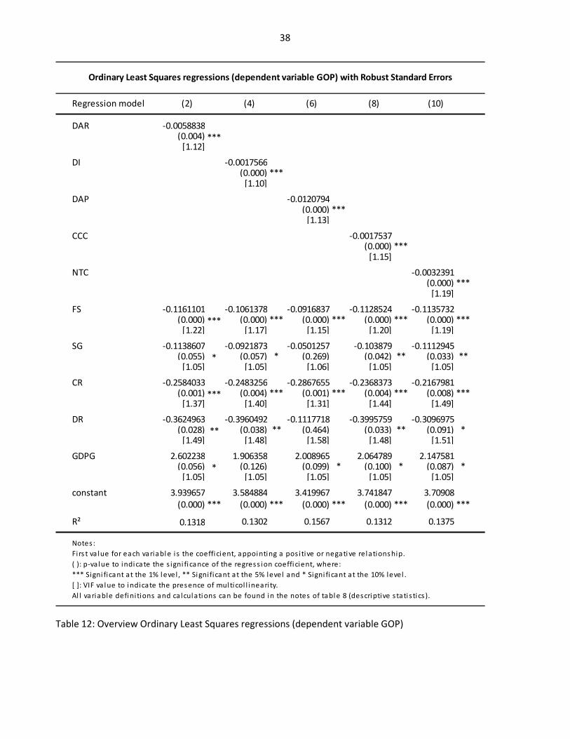
38


DAR -0.0058838(0.004) ***

[1.12]

DI -0.0017566(0.000) ***

[1.10]

DAP -0.0120794(0.000) ***

[1.13]

CCC -0.0017537(0.000) ***

[1.15]

NTC -0.0032391(0.000) ***

[1.19]

FS -0.1161101 -0.1061378 -0.0916837 -0.1128524 -0.1135732(0.000) *** (0.000) *** (0.000) *** (0.000) *** (0.000) ***

[1.22] [1.17] [1.15] [1.20] [1.19]

SG -0.1138607 -0.0921873 -0.0501257 -0.103879 -0.1112945(0.055) * (0.057) * (0.269) (0.042) ** (0.033) **

[1.05] [1.05] [1.06] [1.05] [1.05]

CR -0.2584033 -0.2483256 -0.2867655 -0.2368373 -0.2167981(0.001) *** (0.004) *** (0.001) *** (0.004) *** (0.008) ***

[1.37] [1.40] [1.31] [1.44] [1.49]

DR -0.3624963 -0.3960492 -0.1117718 -0.3995759 -0.3096975(0.028) ** (0.038) ** (0.464) (0.033) ** (0.091) *

[1.49] [1.48] [1.58] [1.48] [1.51]

GDPG 2.602238 1.906358 2.008965 2.064789 2.147581(0.056) * (0.126) (0.099) * (0.100) * (0.087) *

[1.05] [1.05] [1.05] [1.05] [1.05]

constant 3.939657 3.584884 3.419967 3.741847 3.70908

(0.000) *** (0.000) *** (0.000) *** (0.000) *** (0.000) ***

R² 0.1318 0.1302 0.1567 0.1312 0.1375




Ordinary Least Squares regressions (dependent variable GOP) with Robust Standard Errors

Notes :



Table 12: Overview Ordinary Least Squares regressions (dependent variable GOP)

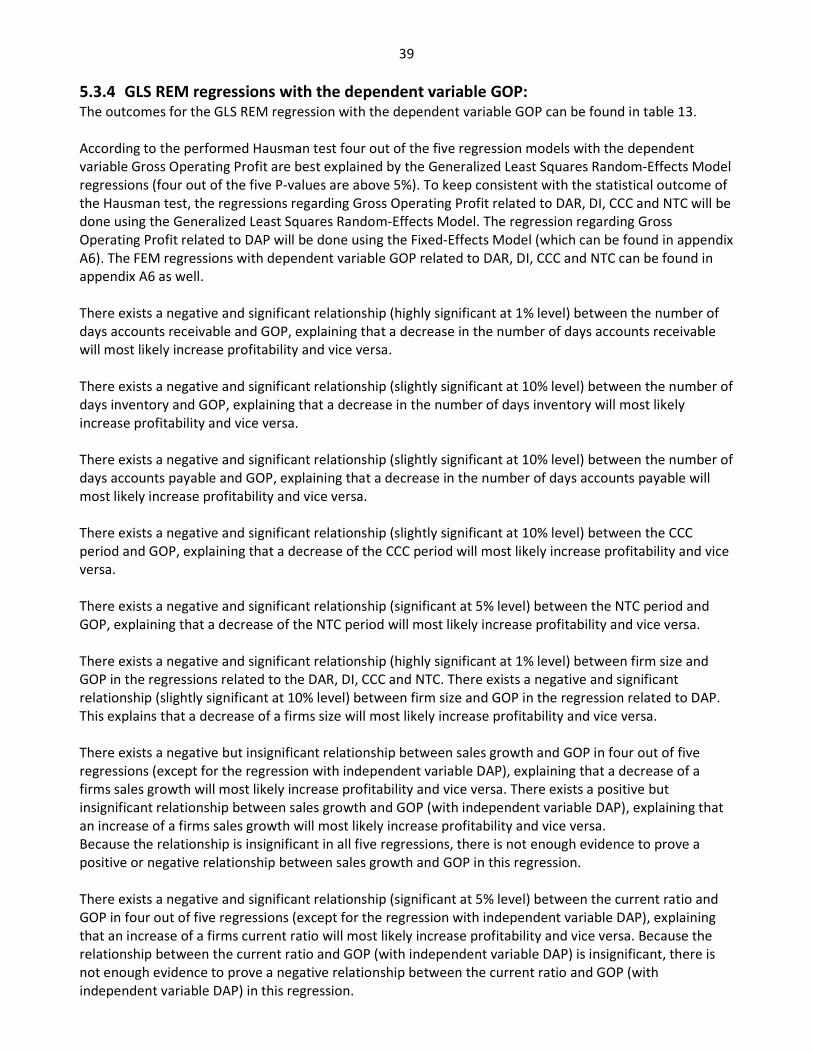
39

5.3.4 GLS REM regressions with the dependent variable GOP: The outcomes for the GLS REM regression with the dependent variable GOP can be found in table 13.

According to the performed Hausman test four out of the five regression models with the dependent

variable Gross Operating Profit are best explained by the Generalized Least Squares Random-Effects Model

regressions (four out of the five P-values are above 5%). To keep consistent with the statistical outcome of

the Hausman test, the regressions regarding Gross Operating Profit related to DAR, DI, CCC and NTC will be

done using the Generalized Least Squares Random-Effects Model. The regression regarding Gross

Operating Profit related to DAP will be done using the Fixed-Effects Model (which can be found in appendix

A6). The FEM regressions with dependent variable GOP related to DAR, DI, CCC and NTC can be found in

appendix A6 as well.

There exists a negative and significant relationship (highly significant at 1% level) between the number of

days accounts receivable and GOP, explaining that a decrease in the number of days accounts receivable


There exists a negative and significant relationship (slightly significant at 10% level) between the number of

days inventory and GOP, explaining that a decrease in the number of days inventory will most likely

increase profitability and vice versa.

There exists a negative and significant relationship (slightly significant at 10% level) between the number of

days accounts payable and GOP, explaining that a decrease in the number of days accounts payable will


There exists a negative and significant relationship (slightly significant at 10% level) between the CCC

period and GOP, explaining that a decrease of the CCC period will most likely increase profitability and vice

versa.

There exists a negative and significant relationship (significant at 5% level) between the NTC period and

GOP, explaining that a decrease of the NTC period will most likely increase profitability and vice versa.

There exists a negative and significant relationship (highly significant at 1% level) between firm size and

GOP in the regressions related to the DAR, DI, CCC and NTC. There exists a negative and significant

relationship (slightly significant at 10% level) between firm size and GOP in the regression related to DAP.

This explains that a decrease of a firms size will most likely increase profitability and vice versa.

There exists a negative but insignificant relationship between sales growth and GOP in four out of five

regressions (except for the regression with independent variable DAP), explaining that a decrease of a

firms sales growth will most likely increase profitability and vice versa. There exists a positive but

insignificant relationship between sales growth and GOP (with independent variable DAP), explaining that

an increase of a firms sales growth will most likely increase profitability and vice versa.

Because the relationship is insignificant in all five regressions, there is not enough evidence to prove a

positive or negative relationship between sales growth and GOP in this regression.

There exists a negative and significant relationship (significant at 5% level) between the current ratio and

GOP in four out of five regressions (except for the regression with independent variable DAP), explaining

that an increase of a firms current ratio will most likely increase profitability and vice versa. Because the

relationship between the current ratio and GOP (with independent variable DAP) is insignificant, there is

not enough evidence to prove a negative relationship between the current ratio and GOP (with

independent variable DAP) in this regression.

40

There exists a negative but insignificant relationship between the debt ratio and GOP in all five regressions,

explaining that an decrease of a firms debt ratio will most likely increase profitability and vice versa.

Because the relationship is insignificant, there is not enough evidence to prove a negative relationship

between the debt ratio and GOP in this regression.

There exists a positive but insignificant relationship between the growth of the annual GDP and GOP in all

five regressions, explaining that an increase of the growth of the annual GDP will most likely increase

profitability and vice versa. Because the relationship is insignificant, there is not enough evidence to prove

a positive relationship between the growth of the annual GDP and GOP in this regression.

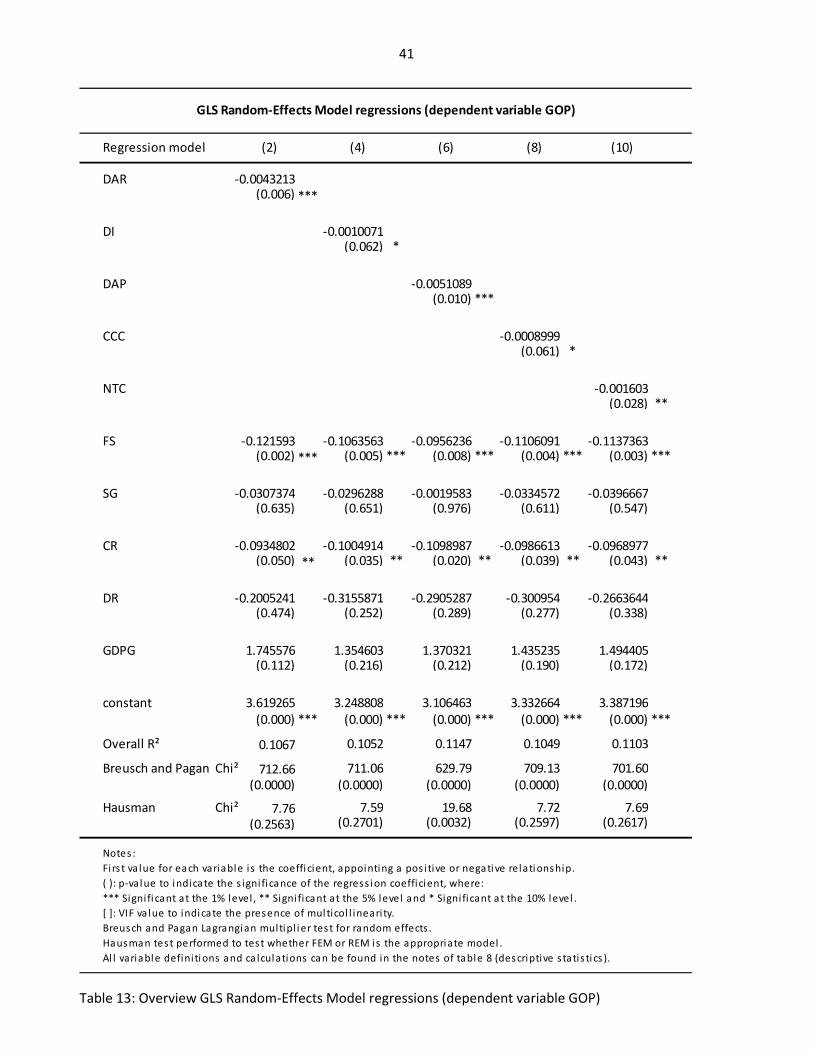
41


DAR -0.0043213(0.006) ***

DI -0.0010071(0.062) *

DAP -0.0051089(0.010) ***

CCC -0.0008999(0.061) *

NTC -0.001603(0.028) **

FS -0.121593 -0.1063563 -0.0956236 -0.1106091 -0.1137363(0.002) *** (0.005) *** (0.008) *** (0.004) *** (0.003) ***

SG -0.0307374 -0.0296288 -0.0019583 -0.0334572 -0.0396667(0.635) (0.651) (0.976) (0.611) (0.547)

CR -0.0934802 -0.1004914 -0.1098987 -0.0986613 -0.0968977(0.050) ** (0.035) ** (0.020) ** (0.039) ** (0.043) **

DR -0.2005241 -0.3155871 -0.2905287 -0.300954 -0.2663644(0.474) (0.252) (0.289) (0.277) (0.338)

GDPG 1.745576 1.354603 1.370321 1.435235 1.494405(0.112) (0.216) (0.212) (0.190) (0.172)

constant 3.619265 3.248808 3.106463 3.332664 3.387196

(0.000) *** (0.000) *** (0.000) *** (0.000) *** (0.000) ***

Overall R² 0.1067 0.1052 0.1147 0.1049 0.1103

Breusch and Pagan Chi² 712.66 711.06 629.79 709.13 701.60

(0.0000) (0.0000) (0.0000) (0.0000) (0.0000)

Hausman Chi² 7.76 7.59 19.68 7.72 7.69

(0.2563) (0.2701) (0.0032) (0.2597) (0.2617)

Breusch and Pagan Lagrangi an multipl i er test for random effects .

Hausman test performed to test whether FEM or REM is the appropri ate model .

Al l variabl e defini ti ons and ca lcul ations can be found in the notes of table 8 (descriptive s tatis ti cs ).

GLS Random-Effects Model regressions (dependent variable GOP)

Notes :

Firs t va lue for each variable is the coeffi cient, appointing a pos itive or negati ve relati onship.

( ): p-val ue to i ndicate the s igni fi cance of the regress i on coeffici ent, where:

*** Signi fi cant at the 1% level , ** Signi ficant at the 5% level and * Signi ficant at the 10% l evel .

[ ]: VIF va lue to indi cate the presence of mul ticol l ineari ty.

Table 13: Overview GLS Random-Effects Model regressions (dependent variable GOP)

42

5.4 Relationships After testing the relationships between the different variables with a correlation and regression analyses in

the previous paragraphs, this paragraph explains the found relationships. An overview of the found

relationships can be found in table 14 below.

DAR Negative *** Negative *** Negative ** Negative *** Negative * Negative ***

DI Negative * Negative *** Negative Negative *** Negative *** Negative *

DAP Negative *** Negative *** Negative ** Negative *** Negative Negative *

CCC Negative ** Negative *** Negative Negative *** Negative *** Negative *

NTC Negative *** Negative *** Negative * Negative *** Negative *** Negative **

FS Positive * Negative *** Positive *** Negative *** Positive * Negative ***

SG Positive *** Negative Positive Negative * Positive *** Negative

CR Positive *** Negative *** Positive *** Negative *** Positive *** Negative **

DR Negative *** Negative Negative *** Negative * Negative *** Negative

GDPG Positive *** Positive Positive *** Positive * Positive *** Positive

is an outcome of the FEM regression as found in appendix 6 (due to the outcome of the Hausman test).

DependentROA

Ind

ep

en

de

nt

va

ria

ble

s

All variable definitions and calculations can be found in the notes of table 8 (descriptive statistics).

variables

REM

regression

FEM

regression

OLS regressions

(Robust Standard Error)

The REM regression outcome for dependent variable GOP related to DAP,

GOP GOP

Overview relationships between variables

Notes:*** Significant at the 1% level, ** Significant at the 5% level and * Significant at the 10% level.

Pearson correlation

ROA GOP ROA

Table 14: Overview relationships between variables

Hypothesis 1: “There is a negative relationship between the number of days accounts receivable and the

profitability of Dutch listed firms”.

The relationship between ROA and DAR and the relationship between GOP and DAR is negative and

significant in the correlation and the regressions. A negative relationship was expected in the hypothesis.

This concludes that we accept the hypothesis and that there is a negative relationship between the

number of days accounts receivable and the profitability of the Dutch listed firms used in this sample. It

seems plausible that the outcome for this research is applicable to other researches as well. The outcome

is consistent with the outcome of (Deloof (2003); Lazaridis and Tryfonidis (2006); Padachi (2006); García-

Teruel and Martínez-Solano (2007); Raheman and Nasr (2007); Gill et al. (2010); Mathuva (2010); Afeef

(2011); Alipour (2011); Ashraf (2012); Kaddumi and Ramadan (2012); Majeed et al. (2013)), and indicates

that an increase in the number of days accounts receivable will decrease profitability and vice versa. It

seems that the Dutch listed firms in this sample that do provide trade credit to their customers are less

profitable than the Dutch listed firms in this sample that do not provide trade credit to their customers.

Firms not providing generous trade credit are less exposed to risk of never paying accounts receivable and

face less liquidity problems and cash flow problems. Firms with higher profits that do want to provide

generous trade credit do not need external financing to finance accounts receivable, and thus have less

impact on firm profitability. Trade credit can be used as a tool to win customers and/or gain large orders,

43

and thus increase sales. For the majority of this dataset, providing more trade credit does not lead to

higher profitability.

Hypothesis 1: Accepted for this research.

Hypothesis 2: “There is a negative relationship between the number of days inventory and the profitability

of Dutch listed firms”.

The relationship between ROA and DI and the relationship between GOP and DI is negative and significant

in the correlation and the regressions. A negative relationship was expected in the hypothesis. This

concludes that we accept the hypothesis and that there is a negative relationship between the number of

days inventory and the profitability of the Dutch listed firms used in this sample. It seems plausible that the

outcome for this research is applicable to other researches as well. The outcome is consistent with the

outcome of (Deloof (2003); Lazaridis and Tryfonidis (2006); Padachi (2006); García-Teruel and Martínez-

Solano (2007); Raheman and Nasr (2007); Afeef (2011); Alipour (2011); Ching et al. (2011); Sharma and

Kumar (2011); Ashraf (2012); Kaddumi and Ramadan (2012); Majeed et al. (2013)), and indicates that an

increase in the number of days inventory will decrease profitability and vice versa. It seems that the Dutch

listed firms in this sample that keep high levels of inventory in stock are less profitable than the Dutch

listed firms in this sample that do not keep high levels of inventory in stock. Firms not keeping high levels

of inventory in stock avoid the risk of not selling inventories and avoid additional costs for warehousing,

insurance and security. Firms that keep high levels of inventory in stock reduce the risk of stock-out, the

cost of possible interruptions in the production process, the possibility of losing business due to the

scarcity of products, the costs for supplying inventory and protects against price fluctuations. For the

majority of this dataset, keeping (too) high levels of inventory does not lead to higher profitability.


Hypothesis 3: “There is a positive relationship between the number of days accounts payable and the


The relationship between ROA and DAP and the relationship between GOP and DAP is negative and

significant in the correlation and all the regressions (except for the FEM regression with dependent

variable ROA). The outcome is consistent with the outcome of (Mathuva (2010); Alipour (2011); Kaddumi

and Ramadan (2012)). A positive relationship was expected in the hypothesis. Following the correlations,

regressions and previous research we reject the hypothesis and conclude that there is a negative

relationship between the number of days accounts payable and the profitability of the Dutch listed firms

used in this sample. It seems plausible that the outcome for this research is applicable to other researches

as well. The negative relationship indicates that an increase in the number of days accounts payable will

decrease profitability and vice versa. It seems that the Dutch listed firms in this sample that postpone to

pay their bills are less profitable than the Dutch listed firms in this sample that do pay their bills on a

shorter notice.

Firms delaying payments to suppliers can assess the quality of bought products and/or services, and it can

be an inexpensive and flexible source of financing for the firm. Firms paying their bills in time can benefit

from discounts if offered, and it can strengthen their long-term relationship with suppliers. For the

majority of this dataset, postponing payments does not lead to higher profitability.

Hypothesis 3: Rejected for this research.

Hypothesis 4: “There is a negative relationship between the cash conversion cycle period and the


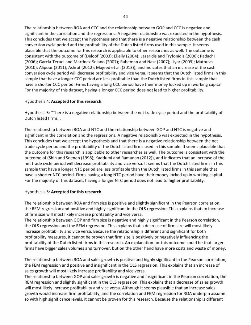
44

The relationship between ROA and CCC and the relationship between GOP and CCC is negative and


This concludes that we accept the hypothesis and that there is a negative relationship between the cash

conversion cycle period and the profitability of the Dutch listed firms used in this sample. It seems

plausible that the outcome for this research is applicable to other researches as well. The outcome is

consistent with the outcome of (Deloof (2003); Eljelly (2004); Lazaridis and Tryfonidis (2006); Padachi

(2006); García-Teruel and Martínez-Solano (2007); Raheman and Nasr (2007); Uyar (2009); Mathuva

(2010); Alipour (2011); Ashraf (2012); Majeed et al. (2013)), and indicates that an increase of the cash

conversion cycle period will decrease profitability and vice versa. It seems that the Dutch listed firms in this

sample that have a longer CCC period are less profitable than the Dutch listed firms in this sample that

have a shorter CCC period. Firms having a long CCC period have their money locked up in working capital.

For the majority of this dataset, having a longer CCC period does not lead to higher profitability.


Hypothesis 5: “There is a negative relationship between the net trade cycle period and the profitability of

Dutch listed firms”.

The relationship between ROA and NTC and the relationship between GOP and NTC is negative and


This concludes that we accept the hypothesis and that there is a negative relationship between the net

trade cycle period and the profitability of the Dutch listed firms used in this sample. It seems plausible that

the outcome for this research is applicable to other researches as well. The outcome is consistent with the

outcome of (Shin and Soenen (1998); Kaddumi and Ramadan (2012)), and indicates that an increase of the

net trade cycle period will decrease profitability and vice versa. It seems that the Dutch listed firms in this

sample that have a longer NTC period are less profitable than the Dutch listed firms in this sample that

have a shorter NTC period. Firms having a long NTC period have their money locked up in working capital.

For the majority of this dataset, having a longer NTC period does not lead to higher profitability.


The relationship between ROA and firm size is positive and slightly significant in the Pearson correlation,

the REM regression and positive and highly significant in the OLS regression. This explains that an increase

of firm size will most likely increase profitability and vice versa.

The relationship between GOP and firm size is negative and highly significant in the Pearson correlation,

the OLS regression and the REM regression. This explains that a decrease of firm size will most likely

increase profitability and vice versa. Because the relationship is different and significant for both

profitability measures, it cannot be proven that firm size is positively or negatively influencing the

profitability of the Dutch listed firms in this research. An explanation for this outcome could be that larger

firms have bigger sales volumes and turnover, but on the other hand have more costs and waste of money.

The relationship between ROA and sales growth is positive and highly significant in the Pearson correlation,

the FEM regression and positive and insignificant in the OLS regression. This explains that an increase of

sales growth will most likely increase profitability and vice versa.

The relationship between GOP and sales growth is negative and insignificant in the Pearson correlation, the

REM regression and slightly significant in the OLS regression. This explains that a decrease of sales growth

will most likely increase profitability and vice versa. Although it seems plausible that an increase sales

growth would increase firm profitability, and the correlation and FEM regression for ROA underpin assume

so with high significance levels, it cannot be proven for this research. Because the relationship is different

45

and some are insignificant for both profitability measures, it cannot be proven that sales growth is

positively or negatively influencing the profitability of the Dutch listed firms in this research.

The relationship between ROA and the current ratio is positive and highly significant in the Pearson

correlation, the OLS regression and the FEM regression. This explains that an increase of the current ratio


The relationship between GOP and the current ratio is negative and highly significant in the Pearson

correlation, the OLS regression and negative and significant in the REM regression. This explains that a

decrease of the current ratio will most likely increase profitability and vice versa.

Because the relationship is different and significant for both profitability measures, it cannot be proven

that the current ratio is positively or negatively influencing the profitability of the Dutch listed firms in this

research. An explanation for the different relationships with the profitability measures could be the

differences in the calculation of the assets part in both measures. The ROA calculation is based on the

average total assets, where the GOP is based on total assets minus financial assets.

The relationship between ROA and the debt ratio is negative and highly significant in the Pearson

correlation, the OLS regression and the FEM regression. This explains that a decrease of the debt ratio will


The relationship between GOP and the debt ratio is negative but insignificant in the Pearson correlation,

the REM regression and negative and slightly significant in the OLS regression. This explains that a decrease

of the debt ratio will most likely increase profitability and vice versa.

Because all outcomes are negative and highly significant for profitability measure ROA and partly

significant for GOP, the assumption can be made that a decrease of the debt ratio will increase profitability

and vice versa for the Dutch listed firms in this research. This seems obvious for the majority of firms, while

debt increases interest costs and thus shorten profitability. In other situations firms need debt to stay in

business, and debt contributes to making profit. An explanation for the insignificant outcome with

profitability measure GOP could be that the calculation is based on total assets minus financial assets,

where the ROA calculation is based on the average total assets.

The relationship between ROA and the annual GDP growth is positive and highly significant in the Pearson

correlation, the OLS regression and the FEM regression. This explains that an increase of the debt ratio will


The relationship between GOP and the debt ratio is positive but insignificant in the Pearson correlation,

the REM regression and positive and slightly significant in the OLS regression. This explains that an increase

of the debt ratio will most likely increase profitability and vice versa.

Because all outcomes assume a positive and highly significant relationship for ROA and a positive and

partly significant relationship for GOP between the profitability variables and annual GDP growth, the

assumption can be made that an increase of the annual GDP growth will increase profitability and vice

versa for the Dutch listed firms in this research. This seems obvious while a positive annual GDP indicates

that customers, industries and the government probably spend/invest more money, and/or that export

probably exceeds import.


“�� ? ”

Answer: Yes. According to the outcome of the correlation and regression analyses, four out of five

hypotheses are accepted for this research. A positive and significant relationship between the number of

days accounts payable and firm profitability was expected. The number of days accounts receivable, the

number of days inventory, the number of days accounts payable, the cash conversion cycle and the net

46

trade cycle all have a negative and significant relationship with the profitability of the firms in this research.

The negative and significant relationship explains that a decrease of the number of days accounts

receivable, the number of days inventory, the number of days accounts payable, the cash conversion cycle

and the net trade cycle most likely increase the profitability of the firms in this research. This concludes

that working capital management does affect the profitability of the Dutch listed firms in this research.

47

6. Conclusions In this chapter the main contents and conclusions on the empirical findings of this research will be

summarized. The conclusions should provide a recommendation for the Dutch listed firms used in this

research, but it seems plausible that the findings of this research relate to non-financial listed firms

worldwide.


“�� ? ”

According to the outcome of the correlation and regression analyses, four out of five hypotheses are

accepted for this research. The hypotheses, the outcomes and the recommendations are drawn below.

Hypothesis 1: There is a negative relationship between the number of days accounts receivable and the


This hypothesis is accepted. As there exists a negative and significant relationship between the number of

days accounts receivable and firm profitability, the firms in this research should try to get their money

from their customers as fast as possible to increase firm profitability. The negative relationship indicates

that an increase in the number of days accounts receivable, decreases firm profitability and vice versa.

Methods for speeding up payments and decreasing the number of days accounts receivable are offering

discounts to in advance or quick paying customers and charge customers that are overdue. To avoid even

more risk, firms should offer various discount percentages associated with various payment periods.

Hypothesis 2: There is a negative relationship between the number of days inventory and the profitability


This hypothesis is accepted. As there exists a negative and significant relationship between the number of

days inventory and firm profitability, the firms in this research should try to keep as less inventory in stock

as possible to increase firm profitability. The negative relationship indicates that an increase in the number

of days inventory, decreases firm profitability and vice versa. Methods for keeping as less money involved

with inventories as possible are using economic order quantity, just-in-time management or even a

supplier-to-customer flow for inventories and trying to use more semi-finished products in the production

process.

Hypothesis 3: There is a positive relationship between the number of days accounts payable and the


This hypothesis is rejected. As there exists a negative and significant relationship between the number of

days accounts payable and firm profitability, the firms in this research should try to complete payments as

soon as possible to make use of early payment discounts when offered. The negative relationship indicates

that an increase in the number of days accounts payable, decreases firm profitability and vice versa. When

no early payment discounts are offered it is recommended to make use of this flexible source as a

substitute for external financing. This could save interest costs for external financing but can harm long-

term relationship with suppliers.

Hypothesis 4: There is a negative relationship between the cash conversion cycle period and the


48

Hypothesis 5: There is a negative relationship between the net trade cycle period and the profitability of

Dutch listed firms.

Both, hypothesis 4 and 5 are accepted. The three components mentioned above form the CCC and NTC, for

both there exists a negative and significant relationship with firm profitability. The negative relationship

indicates that an increase of the CCC and/or NTC period, decreases firm profitability and vice versa. The

firms in this research should try to keep the length of the CCC and NTC period as short as possible.

There is no evidence that firm size, sales growth and current ratio are positively or negatively related to

firm profitability. There exists a negative and significant relationship between debt ratio and firm

profitability and a positive and significant relationship between the annual GDP growth rate and firm

profitability.

The number of days accounts receivable, the number of days inventory, the number of days accounts

payable, the cash conversion cycle and the net trade cycle all have a negative and significant relationship

with the profitability of the firms in this research. The negative and significant relationship explains that a

decrease of the number of days accounts receivable, the number of days inventory, the number of days

accounts payable, the cash conversion cycle and the net trade cycle most likely increase the profitability of

the firms in this research. This concludes that working capital management does affect the profitability of

the Dutch listed firms in this research.

The outcomes are consistent with the majority of the reviewed literature and therefor it seems to be

generalizable to the majority of non-financial listed firms worldwide.

Motivation and extending current literature:

This research can be used as a foundation for existing research as well as for future research on the

relationship between WCM and firm profitability. This research extends existing research with a research

based on more than one dependent variable as a measurement for profitability with the same dataset, as

well as with using the CCC and NTC as independent variables in one research. Furthermore, this research

focuses on Dutch listed firms where limited research has been done to test the relationship between WCM

and firm profitability.

Limitations and recommendations for future research:

This research excludes non-listed firms and financial related firms (banking and insurance). Future research

should include non-listed firms and financial related firms to make the outcomes of the researches

generalizable to all firms worldwide. This research only tried to find the relationship between WCM and

firm profitability. It did not discuss an optimum level for WCM. Future research should try to find the

optimum level for the individual components of WCM to reach the highest firm profitability. Furthermore,

this research based the outcomes on data for Dutch listed firms only. Future research should try to base

one research on the data for multiple countries to see if there exists a relationship between country

specific factors (country specific annual GDP, country specific population count, etc.) and firm profitability.

Note: all outcomes of this research apply to this research setting, the outcomes only make it more

plausible that the outcomes of existing and future research are most likely true or false.

49

Bibliography

1. Afeef, M. (2011). Analyzing the Impact of Working Capital Management on the Profitability of SME’s in

Pakistan.

2. Alipour, M. (2011). Working capital management and corporate profitability: Evidence from Iran. World

applied sciences journal, 12(7), 1093-1099.

3. Ashraf, C. K. (2012). The Relationship between Working Capital Efficiency and Profitability. Advances In

Management Vol, 5, 12.

4. Baños-Caballero, S., García-Teruel, P. J., & Martínez-Solano, P. (2012). How does working capital

management affect the profitability of Spanish SMEs? Small Business Economics, 39(2), 517-529.

5. Charitou, M., Lois, P., & Santoso, H. B. (2012). The Relationship Between Working Capital Management

And Firm’s Profitability: An Empirical Investigation For An Emerging Asian Country. International

Business & Economics Research Journal (IBER), 11(8), 839-848.

6. Ching, H. Y., Novazzi, A., & Gerab, F. (2011). Relationship between working capital management and

profitability in Brazilian listed companies. journal of global business and economics, 3(1), 74-86.

7. Deloof, M. (2003). Does working capital management affect profitability of Belgian firms? Journal of

Business Finance & Accounting, 30(3-4), 573-588.

8. Eljelly, A. M. A. (2004). Liquidity-profitability tradeoff: an empirical investigation in an emerging market.

International Journal of Commerce and Management, 14(2), 48-61.

9. García-Teruel, P. J., & Martínez-Solano, P. (2007). Effects of working capital management on SME

profitability. International Journal of Managerial Finance, 3(2), 164-177.

10. Gill, A., Biger, N., & Mathur, N. (2010). The relationship between working capital management and

profitability: evidence from The United States. Business and Economics Journal, 10, 1-9.

11. Gitman, L. J. (1974). Estimating corporate liquidity requirements: a simplified approach. Financial

Review, 9(1), 79-88.

12. Jose, M. L., Lancaster, C., & Stevens, J. L. (1996). Corporate returns and cash conversion cycles. Journal

of Economics and Finance, 20(1), 33-46.

13. Kaddumi, T. A., & Ramadan, I. Z. (2012). Profitability and Working Capital Management: The Jordanian

Case. International Journal of Economics and Finance, 4(4), p217.

14. Knauer, T., & Wöhrmann, A. (2013). Working capital management and firm profitability. Journal of

Management Control, 1-11.

15. Lazaridis, I., & Tryfonidis, D. (2006). Relationship between working capital management and

profitability of listed companies in the Athens stock exchange. Journal of financial management and

analysis, 19(1).

16. Leach, J. C., & Melicher, R. W. (2011). Entrepreneurial Finance: South-Western Cengage Learning.

17. Majeed, S., Makki, M. A. M., Saleem, S., & Aziz, T. (2013). The Relationship of Cash Conversion Cycle

and Profitability of Firms: An Empirical Investigation of Pakistani Firms.

18. Mathuva, D. (2010). The influence of working capital management components on corporate

profitability: a survey on Kenyan listed firms. Research Journal of Business Management, 3(1), 1-11.

19. Padachi, K. (2006). Trends in working capital management and its impact on firms’ performance: an

analysis of Mauritian small manufacturing firms. International Review of Business Research Papers,

2(2), 45-58.

20. Raheman, A., & Nasr, M. (2007). Working capital management and profitability–case of Pakistani firms.

International Review of Business Research Papers, 3(1), 279-300.

21. Richards, V. D., & Laughlin, E. J. (1980). A cash conversion cycle approach to liquidity analysis. Financial

Management, 32-38.

22. Sharma, A. K., & Kumar, S. (2011). Effect of Working Capital Management on Firm Profitability Empirical

Evidence from India. Global Business Review, 12(1), 159-173.

23. Shin, H.-H., & Soenen, L. (1998). Efficiency of working capital management and corporate profitability.

Financial Practice and Education, 8, 37-45.

24. Smith, K. V. (1980). Readings on the management of working capital: West Publishing Company.

50

25. Sutton, T. (2004). Corporate Financial Accounting and Reporting: FT Prentice Hall/ Financial Times.

26. Uyar, A. (2009). The relationship of cash conversion cycle with firm size and profitability: an empirical

investigation in Turkey. International Research Journal of Finance and Economics, 24(2), 186-193.

27. ORBIS database by Bureau van Dijk, Retrieved Januar 21, 2014, from https://orbis.bvdinfo.com/ip/

28. World Bank database, Retrieved Januar 29, 2014, from http://data.worldbank.org/

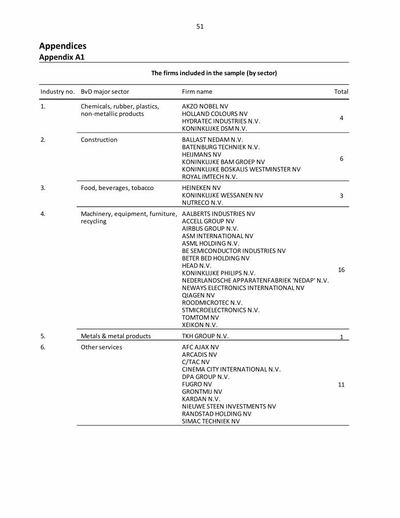
51

Appendices Appendix A1

Industry no. BvD major sector Firm name Total

1. Chemicals, rubber, plastics, AKZO NOBEL NVnon-metallic products HOLLAND COLOURS NV

HYDRATEC INDUSTRIES N.V.KONINKLIJKE DSM N.V.

2. Construction BALLAST NEDAM N.V.BATENBURG TECHNIEK N.V.HEIJMANS NVKONINKLIJKE BAM GROEP NVKONINKLIJKE BOSKALIS WESTMINSTER NVROYAL IMTECH N.V.

3. Food, beverages, tobacco HEINEKEN NVKONINKLIJKE WESSANEN NVNUTRECO N.V.

4. Machinery, equipment, furniture, AALBERTS INDUSTRIES NVrecycling ACCELL GROUP NV

AIRBUS GROUP N.V.ASM INTERNATIONAL NVASML HOLDING N.V.BE SEMICONDUCTOR INDUSTRIES NVBETER BED HOLDING NVHEAD N.V.KONINKLIJKE PHILIPS N.V.NEDERLANDSCHE APPARATENFABRIEK 'NEDAP' N.V.NEWAYS ELECTRONICS INTERNATIONAL NVQIAGEN NVROODMICROTEC N.V.STMICROELECTRONICS N.V.TOMTOM NVXEIKON N.V.

5. Metals & metal products TKH GROUP N.V. 1

6. Other services AFC AJAX NVARCADIS NVC/TAC NVCINEMA CITY INTERNATIONAL N.V.DPA GROUP N.V.FUGRO NVGRONTMIJ NVKARDAN N.V.NIEUWE STEEN INVESTMENTS NVRANDSTAD HOLDING NVSIMAC TECHNIEK NV

4

The firms included in the sample (by sector)

11

16

3

6

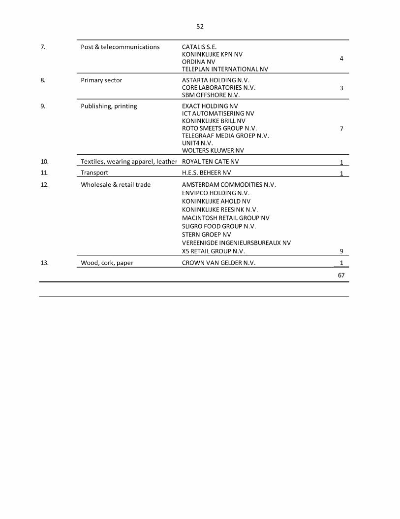
52

7. Post & telecommunications CATALIS S.E.KONINKLIJKE KPN NVORDINA NVTELEPLAN INTERNATIONAL NV

8. Primary sector ASTARTA HOLDING N.V.CORE LABORATORIES N.V.SBM OFFSHORE N.V.

9. Publishing, printing EXACT HOLDING NVICT AUTOMATISERING NVKONINKLIJKE BRILL NVROTO SMEETS GROUP N.V.TELEGRAAF MEDIA GROEP N.V.UNIT4 N.V.WOLTERS KLUWER NV

10. Textiles, wearing apparel, leather ROYAL TEN CATE NV 1

11. Transport H.E.S. BEHEER NV 1

12. Wholesale & retail trade AMSTERDAM COMMODITIES N.V.

ENVIPCO HOLDING N.V.

KONINKLIJKE AHOLD NV

KONINKLIJKE REESINK N.V.

MACINTOSH RETAIL GROUP NV

SLIGRO FOOD GROUP N.V.

STERN GROEP NV

VEREENIGDE INGENIEURSBUREAUX NV

X5 RETAIL GROUP N.V.

13. Wood, cork, paper CROWN VAN GELDER N.V. 1

67

9

7

3

4

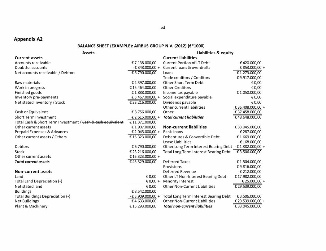
53

Appendix A2

Current assets Current liabilitiesAccounts receivable € 7.138.000,00 Current Portion of LT Debt € 420.000,00Doubtful accounts -€ 348.000,00 + Current loans & overdrafts € 853.000,00 +

Net accounts receivable / Debtors € 6.790.000,00 Loans € 1.273.000,00Trade creditors / Creditors € 9.917.000,00

Raw materials € 2.397.000,00 Other Short Term Debt € 0,00Work in progress € 15.464.000,00 Other Creditors € 0,00Finished goods € 1.888.000,00 Income tax payable € 1.050.000,00Inventory pre-payments € 3.467.000,00 + Social expenditure payable € 0,00

Net stated inventory / Stock € 23.216.000,00 Dividends payable € 0,00Other current liabilities € 36.408.000,00 +

Cash or Equivalent € 8.756.000,00 Other € 37.458.000,00

Short Term Investment € 2.615.000,00 + Total current liabilities € 48.648.000,00Total Cash & Short Term Investment / Cash & cash equivalent € 11.371.000,00Other current assets € 1.907.000,00 Non-current liabilities € 33.045.000,00Prepaid Expenses & Advances € 2.045.000,00 + Bank Loans € 287.000,00

Other current assets / Others € 15.323.000,00 Debentures & Convertible Debt € 1.669.000,00Lease Liabilities € 168.000,00

Debtors € 6.790.000,00 Other Long Term Interest Bearing Debt € 1.382.000,00 +

Stock € 23.216.000,00 Total Long Term Interest Bearing Debt € 3.506.000,00Other current assets € 15.323.000,00 +

Total current assets € 45.329.000,00 Deferred Taxes € 1.504.000,00Provisions € 9.816.000,00

Non-current assets Deferred Revenue € 212.000,00Land € 0,00 Other LT Non-Interest Bearing Debt € 17.982.000,00Total Land Depreciation (-) € 0,00 + Minority Interest € 25.000,00 +

Net stated land € 0,00 Other Non-Current Liabilities € 29.539.000,00Buildings € 8.542.000,00Total Buildings Depreciation (-) -€ 3.909.000,00 + Total Long Term Interest Bearing Debt € 3.506.000,00Net Buildings € 4.633.000,00 Other Non-Current Liabilities € 29.539.000,00 +

Plant & Machinery € 15.293.000,00 Total non-current liabilities € 33.045.000,00

BALANCE SHEET (EXAMPLE): AIRBUS GROUP N.V. (2012) (€*1000)

Liabilities & equityAssets

54

Plant & Machinery Depreciation (-) -€ 9.422.000,00 +Net Stated Plant & Machinery € 5.871.000,00 Total current liabilities € 48.648.000,00Transportation Equipment € 0,00 Total non-current liabilities € 33.045.000,00

Transportation Equipment Depreciation (-) € 0,00 + Total liabilities & debt € 81.693.000,00Net Transportation Equipment € 0,00Leased Assets € 0,00 EquityLeased Assets Depreciation (-) € 0,00 + Common Stock / Shares / Share Capital € 827.000,00Net Leased Assets € 0,00 Participation Shares € 0,00Other Property Plant & Equipment € 7.287.000,00 Preferred Shares € 0,00Other Property Plant & Equipment Depreciation (-) -€ 2.595.000,00 + Redeemable Prefered Shares € 0,00 +

Net Other Property Plant & Equipment € 4.692.000,00 + Total shares € 827.000,00Accumulated Depreciation, n.e.s. (-) € 0,00 +

Tangible fixed assets / Net Property, Plant & Equipment € 15.196.000,00 Share Premiums € 7.253.000,00Treasury Shares -€ 84.000,00

Goodwill € 11.003.000,00 Revaluation Reserves € 0,00Other Intangibles € 1.054.000,00 + Retained Earnings € 2.129.000,00Intangible fixed assets / Intangibles € 12.057.000,00 Other Shareholders Reserves € 284.000,00 +

Other € 9.582.000,00Exploration € 0,00Long Term Receivables € 0,00 Total Shares € 827.000,00Investments € 9.488.000,00 Other € 9.582.000,00 +

Long Term Associated Companies € 2.662.000,00 Total Shareholders Equity € 10.409.000,00Investment Properties € 72.000,00Other Long Term Assets € 7.298.000,00 +

Other fixed assets € 19.520.000,00

Tangible fixed assets € 15.196.000,00Intangible fixed assets € 12.057.000,00Other fixed assets € 19.520.000,00 +

Total non-current assets / Fixed assets € 46.773.000,00

Current assets € 45.329.000,00 Total liabilities & debt € 81.693.000,00Non-current assets € 46.773.000,00 + Total shareholders equity € 10.409.000,00 +

Total assets € 92.102.000,00 Total liabilities & equity € 92.102.000,00

55

Appendix A3


DAR -0.0006275(0.000) ***

[1.12]

DI -0.0001183(0.012) **

[1.10]

DAP -0.0006644(0.004) ***

[1.13]

CCC -0.0001449(0.002) ***

[1.15]

NTC -0.0003134(0.000) ***

[1.19]

FS 0.0082035 0.0096945 -0.0106237 0.0089738 0.008655(0.000) *** (0.000) *** (0.004) *** (0.000) *** (0.000) ***

[1.22] [1.17] [1.15] [1.20] [1.19]

SG 0.0229949 0.025079 0.0273211 0.0242015 0.0234003(0.029) ** (0.019) ** (0.010) *** (0.023) ** (0.027) **

[1.05] [1.05] [1.06] [1.05] [1.05]

CR 0.0256742 0.0244319 0.0215905 0.0262808 0.0292173(0.000) *** (0.000) *** (0.000) *** (0.000) *** (0.000) ***

[1.37] [1.40] [1.31] [1.44] [1.49]

DR -0.1209719 -0.1317643 -0.1183916 -0.1292538 -0.1180078(0.000) *** (0.000) *** (0.000) *** (0.000) *** (0.000) ***

[1.49] [1.48] [1.58] [1.48] [1.51]

GDPG 0.809714 0.7443619 0.7527861 0.7540074 0.7610701(0.000) *** (0.000) *** (0.000) *** (0.000) *** (0.000) ***

[1.05] [1.05] [1.05] [1.05] [1.05]

constant -0.0694063 -0.1143357 -0.1256325 -0.0986146 -0.0970072

(0.148) (0.014) ** (0.007) *** (0.036) ** (0.037) **

R² 0.1633 0.1483 0.1509 0.1534 0.1628

Adjusted R² 0.1549 0.1397 0.1423 0.1449 0.1544

White's test Chi² 64.67 79.83 75.80 70.42 54.54

(0.0001) (0.0000) (0.0000) (0.0000) (0.0013)


White's tes t performed to test for heteroskedastici ty .

Ordinary Least Squares regressions (dependent variable ROA)

Notes :





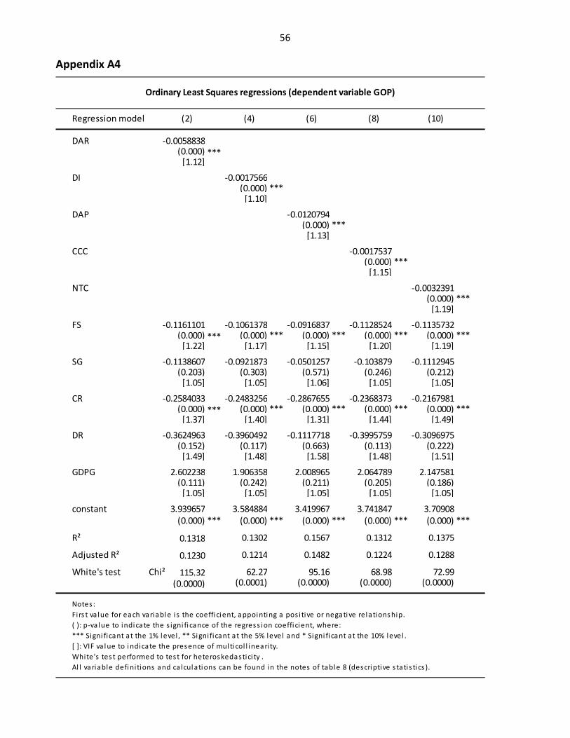
56

Appendix A4


DAR -0.0058838(0.000) ***

[1.12]

DI -0.0017566(0.000) ***

[1.10]

DAP -0.0120794(0.000) ***

[1.13]

CCC -0.0017537(0.000) ***

[1.15]

NTC -0.0032391(0.000) ***

[1.19]

FS -0.1161101 -0.1061378 -0.0916837 -0.1128524 -0.1135732(0.000) *** (0.000) *** (0.000) *** (0.000) *** (0.000) ***

[1.22] [1.17] [1.15] [1.20] [1.19]

SG -0.1138607 -0.0921873 -0.0501257 -0.103879 -0.1112945(0.203) (0.303) (0.571) (0.246) (0.212)

[1.05] [1.05] [1.06] [1.05] [1.05]

CR -0.2584033 -0.2483256 -0.2867655 -0.2368373 -0.2167981(0.000) *** (0.000) *** (0.000) *** (0.000) *** (0.000) ***

[1.37] [1.40] [1.31] [1.44] [1.49]

DR -0.3624963 -0.3960492 -0.1117718 -0.3995759 -0.3096975(0.152) (0.117) (0.663) (0.113) (0.222)

[1.49] [1.48] [1.58] [1.48] [1.51]

GDPG 2.602238 1.906358 2.008965 2.064789 2.147581(0.111) (0.242) (0.211) (0.205) (0.186)

[1.05] [1.05] [1.05] [1.05] [1.05]

constant 3.939657 3.584884 3.419967 3.741847 3.70908

(0.000) *** (0.000) *** (0.000) *** (0.000) *** (0.000) ***

R² 0.1318 0.1302 0.1567 0.1312 0.1375

Adjusted R² 0.1230 0.1214 0.1482 0.1224 0.1288

White's test Chi² 115.32 62.27 95.16 68.98 72.99

(0.0000) (0.0001) (0.0000) (0.0000) (0.0000)



White's tes t performed to test for heteroskedastici ty .


Ordinary Least Squares regressions (dependent variable GOP)

Notes :



57

Appendix A5


DAR -0.0006289(0.002) ***

DI -0.0001889(0.004) ***

DAP -0.0003032(0.264)

CCC -0.0002013(0.001) ***

NTC -0.0003783(0.000) ***

FS 0.0125102 0.0140737 0.0153419 0.0129752 0.012507(0.001) *** (0.000) *** (0.000) *** (0.001) *** (0.001) ***

SG 0.0277585 0.0276433 0.0311598 0.0261164 0.0245201(0.003) *** (0.004) *** (0.001) *** (0.006) *** (0.010) ***

CR 0.0328646 0.0327979 0.0297715 0.0338014 0.0349293(0.000) *** (0.000) *** (0.000) *** (0.000) *** (0.000) ***

DR -0.2233762 -0.2374465 -0.2387812 -0.2330982 -0.2232459(0.000) *** (0.000) *** (0.000) *** (0.000) *** (0.000) ***

GDPG 0.7954795 0.7347765 0.7383821 0.7528776 0.7671845(0.000) *** (0.000) *** (0.000) *** (0.000) *** (0.000) ***

constant -0.1080262 -0.1479137 -0.1754022 -0.1244106 -0.1178313

(0.185) (0.066) (0.024) * (0.126) (0.144)

Overall R² 0.1567 0.1430 0.1406 0.1483 0.1569

Breusch and Pagan Chi² 182.51 198.50 171.26 199.84 198.49

(0.0000) (0.0000) (0.0000) (0.0000) (0.0000)

Hausman test Chi² 33.76 12.90 33.40 48.79 30.83

(0.0000) (0.0446) (0.0000) (0.0000) (0.0000)

Al l variable definitions a nd ca lculations can be found in the notes of ta ble 8 (descriptive statis ti cs ).

Breusch and Paga n Lagra ngian multipl ier tes t for random effects .

Haus man test performed to test whether FEM or REM i s the a ppropriate model .

GLS Random-Effects Model regressions (dependent variable ROA)

Notes:

First va lue for each variable is the coeffi cient, appointing a pos i tive or negative rela tions hip.

( ): p-va lue to indicate the s igni ficance of the regres s ion coeffi cient, where:

*** Signi fi ca nt at the 1% level , ** Signi ficant at the 5% level and * Signi ficant at the 10% level .

[ ]: VIF va lue to indicate the presence of mul ticol l inea ri ty.

58

Appendix A6


DAR -0.0035836(0.048) **

DI -0.0004401(0.495)

DAP -0.0035017(0.100) *

CCC -0.0004158(0.449)

NTC -0.0009171(0.262)

FS -0.1565221 -0.1246236 -0.1240154 -0.1279412 -0.1378389(0.037) ** (0.089) * (0.087) * (0.084) * (0.066) *

SG -0.0166841 -0.0087223 0.006221 -0.0108687 -0.0172731(0.799) (0.896) (0.924) (0.871) (0.796)

CR -0.0651455 -0.0700176 -0.0710854 -0.0693586 -0.069759(0.206) (0.175) (0.168) (0.180) (0.177)

DR -0.2537341 -0.373829 -0.3625363 -0.3626877 -0.3395747(0.412) (0.219) (0.230) (0.235) (0.267)

GDPG 1.464565 1.173674 1.165052 1.208274 1.24054(0.187) (0.287) (0.290) (0.274) (0.261)

constant 4.273986 3.554376 3.611203 3.620496 3.826944

(0.007) *** (0.022) ** (0.018) ** (0.020) ** (0.015) **

Overall R² 0.0809 0.0697 0.0776 0.0699 0.0752

Hausman test Chi² 7.76 7.59 19.68 7.72 7.69

(0.2563) (0.2701) (0.0032) (0.2597) (0.2617)



Hausman test performed to test wether FEM or REM is the appropriate model .


Fixed-Effects Model regressions (dependent variable GOP)

Notes :



Documents

University of Twente Business Administration Financial ...essay.utwente.nl/65105/1/Linderhof_MA_MB.pdf · University of Twente Business Administration ... Financial Management