Embed Size (px)
Citation preview

UNIVERSITY OF TORONTO SCARBOROUGH
Department of Computer and Mathematical Sciences
Midterm Test February 2016
STAB22H3 Statistics I, LEC 01 and LEC 02Duration: 1 hour and 45 minutes
Last Name: First Name:
Student number:
Aids allowed:
- One handwritten letter-sized sheet (both sides) of notes prepared by you
- Non-programmable, non-communicating calculator
Standard normal distribution tables are attached at the end.
This test is based on multiple-choice questions. There are 35 questions. All questions carryequal weight. On the Scantron answer sheet, ensure that you enter your last name, firstname (as much of it as fits), and student number (in “Identification”).
Mark in each case the best answer out of the alternatives given (which means the nu-
merically closest answer if the answer is a number and the answer you obtained
is not given.)
Also before you begin, complete the signature sheet, but sign it only when the invigilatorcollects it. The signature sheet shows that you were present at the exam.
There are 18 pages including this page and statistical tables. Please check to see you haveall the pages.
Good luck!!
Answer Key for Exam A
1

1. Use this information for this question and the next two questions. The length ofhuman pregnancies (with no complications)from conception to birth varies and has anormal distribution with mean 260 days and standard deviation 10. Approximatelywhat percentage of pregnancy lengths are above 285 days?
(a) 0.0062 percent
(b) 0.0250 percent
(c) 0.2500 percent
(d) 0.6200 percent
(e) 0.9938 percent
2. Refer to the information in question 1 above. The longest five percent of the pregnancylengths are, approximately, longer than what value?
(a) 244
(b) 255
(c) 265
(d) 273
(e) 276
3. Refer to the information in question 1 above. Using 68-95-99.7 rule, what percentageof pregnancy lengths are, approximately, between 250 and 280 days?
(a) 68.0
(b) 81.5
(c) 95
(d) 97.5
(e) 99.7
4. If the correlation coefficient (r)= 1.00, then
(a) all the points on the scatter diagram must fall exactly on a straight line with anegative slope.
(b) all the points on the scatter diagram must fall exactly on a straight line with a
positive slope.
(c) all the points on the scatter diagram must fall exactly on a straight line with azero slope.
(d) all the points on the scatter diagram must fall exactly on a straight line withslope equal to 1.
(e) all the points on the scatter diagram must fall close to a straight line but notnecessarily exactly on straight line.
2

5. The gross revenue (in millions of dollars) for the top 20 movies over the 2001 LaborDay Weekend had median 3.85, the first quartile 1.5, and the third quartile 8.4. Thefour lowest observations had gross revenues 1.2, 1.3, 1.7, 1.8, and the three highestobservations had gross revenues 11, 11.7, 15.8. Based on the 1.5 × IQR rule, howmany outliers are there in this data set of gross revenues?
(a) No outliers
(b) Only one outlier
(c) Only two outliers
(d) Only three outliers
(e) More than three outliers
6. A researcher wants to construct the regression equation for predicting grocery bills(BILLS) from number of people in the household (NUMBER). He has calculated theslope to be 33.57. The mean BILL is $132.71 and the mean NUMBER is 2.71. Whatis the value of the y-intercept?
(a) 132.71
(b) 8.2
(c) 41.73
(d) 223.68
(e) 130
7. Three statistics classes (50 students each) took the same test. Shown below are his-tograms of the scores for the classes. Use the histograms to answer the question.
Which class had the highest median score?
(a) Class 1
(b) Class 2
(c) Class 1 and Class 3
(d) Class 3
(e) None, because the classes had the same mean.
3

8. Which of the following values of the correlation r indicates the strongest correlationbetween the two variables?
(a) r = 1.22
(b) r = −1.90
(c) r = 0.75
(d) r = −0.81
(e) r = 1.22
9. In a study, educational researchers were interested in predicting schools AcademyPerformance Index score (y) on the results of the Stanford 9 Achievement test frompercent of students at that school who are considered English Language Learners(x). Scores ranged from 200 to 1000. The researchers took a random sample of eightelementary schools in Riverside County, California, and recorded schools AcademyPerformance Index (API) scores along with the percent of students at that schoolwho are considered English Language Learners (ELL). The scatterplot of y againstx was approximately linear. Use this information for this question and the next fourquestions. The regression equation is: y = 727.22− 2.46x
The estimated coefficient of determination, R2 is 0.79.
Approximately, what is the estimated correlation, r?
(a) 0.40
(b) 0.79
(c) -0.79
(d) 0.89
(e) -0.89
10. Refer to the information in question 9. Which of the following statements is an accurateinterpretation of estimated coefficient of determination, R2 = 0.79 in the context ofthis study.
(a) The percent of students at that school who are considered ELL causes APIscores to increase by 0.79%
(b) About 79% of variation in API scores is explained by the linear regression with
the percent of students at that school who are considered ELL.
(c) About 79% of API scores is explained by the linear regression with the percentof students at that school who are considered ELL.
(d) About 79% of variation in the percent of students who are considered ELL inthese schools is explained by the linear regression with API scores.
(e) About 79% of the percent of students who are considered ELL in these schoolsis explained by the linear regression with API scores.
4

11. Refer to the information in question 9. The slope of the regression line is -2.46. Thismeans that:
(a) When the percentage of students who are considered ELL increases by 1, the
mean API score is estimated to decrease by 2.46.
(b) When the percentage of students who are considered ELL increases by 1, themean API score is estimated to increase by 2.46.
(c) When the API score increases by 1, the mean percentage of students who areconsidered ELL is estimated to increase by 2.46.
(d) When the API score increases by 1, the mean percentage of students who areconsidered ELL is estimated to decrease by 2.46.
(e) The estimated mean API score is -2.46.
12. Refer to the information in question 9. If x = 0 was in the observed range of x values,which of the following statements is true?
(a) The mean percent of students who are considered ELL is estimated to be 0.
(b) There would be no relationship between API scores and the percent of studentswho are considered ELL.
(c) The mean score in API is estimated to be 727.22 when the percentage of students
who are considered ELL is 0.
(d) There would be no meaningful relationship between API scores and the percentof students who are considered ELL.
(e) The mean score in API is estimated to be 0 when the percentage of studentswho are considered ELL is 0.
5

13. In checking the adequacy of the regression model, the plot below shows that:
(a) Residual points are evenly spread out. No major pattern is seen. Thus, theregression model is correct.
(b) Residual points are evenly spread out. No major pattern is seen. Thus, theregression model is incorrect.
(c) Residual points are not evenly spread out. A major pattern is observed. Thus,the regression model is correct.
(d) Residual points are not evenly spread out. A pattern is observed. Thus, the
regression model is incorrect
(e) As x values increases, residual points increases. Thus, regression model is cor-rect.
6

14. The Normal quantile plot of the grades in an exam is shown below.
Based on this information what can we conclude about the distribution of these grades?
(a) The distribution is approximately Normal.
(b) The distribution is right skewed.
(c) The distribution is left skewed.
(d) The distribution is symmetric but not Normal.
(e) The distribution is not symmetric.
15. A study investigated the relationship between GPA scores and MCAT scores (scoreson Medical College Admission Test) for 55 applicants who applied to various medicalschools. The study aimed at predicting MCAT scores (y) from GPA scores (x). Assumethat the scatterplot of y against x is approximately linear.The regression equation is: y = 3.92 + 9.10x.For an applicant in this study, the GPA score is 3.62 and the MCAT score is 38. Whatis the residual for this observation?
(a) 1.14
(b) -1.14
(c) 5.06
(d) -5.06
(e) 346.10
7
16. Which of the following statements about correlation and regression is/are true?
I) Correlation based on data that are summary statistics are usually higher.
II) If r2 = 0.95, then the response variable increases as the explanatory variableincreases.
III) An outlier always decreases the correlation.
(a) Only statement I is true.
(b) Only statements I and II are true.
(c) Only statements II and III are true.
(d) Only statements I and III are true.
(e) All statements I, II and III are true.
8

17. The graph below represents the percentage of workers living in 18 Canadian cities whoused public transportation to commute to work.Note: In order to avoid complications, you may assume that no city in this sample hadpercentage of workers who used public transportation exactly at a class boundary.
Based in this information, which of the following statements is true?
(a) More than 30 percent of workers in this sample used public transportation tocommute to work.
(b) About 22 percent of cities in this sample had more than 30 percent of their
workers who used public transportation to commute to work.
(c) About 4 percent of cities in this sample had more than 30 percent of theirworkers who used public transportation to commute to work
(d) More than 30 percent of cities in this sample had workers who used public
transportation to commute to work.
(e) About 3 percent of cities in this sample had more than 30 percent of theirworkers who used public transportation to commute to work.
18. The distribution for starting salaries in Major League Baseball is highly skewed witha tail to the right.If the median starting income is $500,000 per year, what can be saidabout the mean starting income?
(a) It is less than $500,000 per year.
(b) It is equal to $500,000 per year.
(c) It is greater than $500,000 per year.
(d) It cannot be determined with the given information.
(e) It is equal to the mode.
9

19. The stemplot below shows the annual family incomes (in dollars) of a random sampleof 20 families selected from a city.
Variable: Family Income
Decimal point is 5 digit(s) to the right of the colon.
Leaf unit = 10000
0 : 11222333
0 : 55788899
1 : 022
1 : 7
Use this data to calculate the third quartile (Q3)of the family income.
(a) 20000 dollars
(b) 50000 dollars
(c) 9000 dollars
(d) 5000 dollars
(e) 90000 dollars
20. Which of the following statements about influential and/or high leverage points is/aretrue?
I) Removal of an influential point changes the regression line.
II) All high leverage points are influential.
III) All hight leverage points have large residuals.
(a) Only statement I is true.
(b) Only statements I and II are true.
(c) Only statements II and III are true.
(d) Only statements I and III are true.
(e) All statements I, II and III are true.
10

21. A student in STAB22 did all ten quizzes. The average of the grades of these ten quizzesis 8.0. According to our quiz evaluation policy, we drop the lowest quiz grade and usethe average of the grades of the best nine quizzes. This student’s lowest quiz grade is3.0. If we drop this lowest quiz, what is the average of the grades of the other ninequizzes? (i.e. the average of her best nine quiz grades)?
(a) 8.0
(b) 8.2
(c) 8.6
(d) 9.0
(e) 9.4
22. Which of the following statements regarding the standard deviation is FALSE?
(a) The numbers 7, 7, 7 have a standard deviation of 0.
(b) The numbers 8, 9, 10 have a smaller standard deviation than 1, 3, 5.
(c) The numbers 1, 2, 4, 5 have a smaller standard deviation than 1, 1, 5, 5.
(d) The numbers 1, 2, 3 have a smaller standard deviation than 2, 4, 6.
(e) The numbers 3, 5, 7 have a smaller standard deviation than 103, 105, 107.
11

23. The boxplot of the age (in years) at death of a group of 200 individuals is shown below.
Based in this information, what is the interquartile range of the distribution of the ageat death?
(a) 25 years
(b) 30 years
(c) 55 years
(d) 75 years
(e) 85 years
24. Refer to the information in question 23 above. Based on this information how many
individuals in this sample died before the age of 55 years?Note: In order to avoid complications, you may assume that no one in this sample diedexactly at any of the quartiles.
(a) 50 individuals
(b) 55 individuals
(c) 75 individuals
(d) 80 individuals
(e) 85 individuals
12

25. Refer to the information in question 23 above. Based on this information what can wesay about the shape of the distribution of age at death of these individuals.
(a) The distribution of age at death of these individuals is right skewed.
(b) The distribution of age at death of these individuals is left skewed.
(c) The distribution of age at death of these individuals is symmetric.
(d) The distribution of age at death of these individuals is bell-shaped.
(e) This boxplot gives no information about the shape of the distribution.
26. A social researcher collects the following data from 100 residents in a community. Whatvariable is categorical?
(a) Age (in years)
(b) Level of education
(c) Household income
(d) Years of education
(e) Number of children
27. Use this information for this question and the next three questions. A survey wasconducted to evaluate the effectiveness of a new flu vaccine that had been administratedin a small community. The vaccine was provided free of charge in a two-shot sequenceover a period of 2 weeks. Some people received the two-shot sequence, some appearedfor only the first shot, and others received neither. A survey of 1000 local residents inthe following spring provided the information shown in the table below. The researcherworking on this data was interested to investigate if this vaccine was successful inreducing the number of flu cases in the community.
TreatmentCases of Flu No Vaccine One shot Two shots Total
Flu 24 9 13 46No flu 289 100 565 954Total 313 109 578 1000
Suppose the researcher wants to compare the proportion of residents who had the fluin the following spring among those who received the two-shot sequences, only thefirst shot, and others that received neither. Which percentage should the researchercalculate?
(a) Row percentage
(b) Column percentage
(c) Joint percentage
(d) Marginal percentage
(e) Marginal percentage of those who did not get the flu
13

28. In the study in question 27 above, what is the dependent variable?
(a) Treatment
(b) The residents
(c) The researcher
(d) Whether the residents had the flu or not in the following spring
(e) The effect of no vaccine
29. Refer to the information in question 27 above. What percentage of the residents thatreceived no vaccine had the flu in the following spring?
(a) 4.6
(b) 7.7
(c) 24.0
(d) 31.3
(e) 52.2
30. Refer to the information in question 27 above. Among those residents who receivedeither one shot or two shots, what is the conditional percentage of those who had theflu in the following spring?
(a) 2.2
(b) 3.2
(c) 10.5
(d) 47.8
(e) 68.7
14

31. Twenty-six households were polled in a marketing survey. The graph below shows thenumber of quarts of milk purchased during a particular week.
Variable: Quarts of milk
Decimal point is at the colon.
Leaf unit = 0.1
0 : 00
0 :
1 : 00000
1 :
2 : 000000000
2 :
3 : 00000
3 :
4 : 000
4 :
5 :
5 :
6 : 00
What percentage of households purchased less than 4 quarts of milk during a particularweek?
(a) 12
(b) 21
(c) 24
(d) 81
(e) 92
32. Refer to the information in question 31 above. What is the shape of the distributionof number of quarts of milk purchased during a particular week?
(a) Exactly symmetrical
(b) Right Skewed
(c) Normal
(d) Bell-shaped
(e) Left skewed
15

33. Refer to the information in question 31 above. What is the most appropriate measureof spread for the data on the number of quarts of milk purchased during a particularweek?
(a) Mode
(b) Standard deviation
(c) Variance
(d) Range
(e) Inter Quartile Range
34. Which of the following statements about the Normal density curves is/are true?
I) The total area under the Normal density curve (and above the horizontal line(i.e. density = 0 line ) ) is 1.
II) All Normal density curves are bell-shaped.
III) All bell-shaped density curves are Normal density curves.
(a) Only statement I is true.
(b) Only statements I and II are true.
(c) Only statements II and III are true.
(d) Only statements I and III are true.
(e) All statements I, II and III are true.
35. The survey of Teachers Attitude Toward Computers asked teachers to indicate theirfeelings about working with computers as Strongly Disagree, Disagree, Undecided,Agree, or Strongly Agree. What type of a variable is this?
(a) A categorical variable measured on a nominal scale.
(b) A quantitative variable measured on an interval scale
(c) A categorical variable measured on an ordinal scale.
(d) A quantitative variable measured on a nominal scale
(e) A categorical variable measured on an interval scale.
16
Tables of normal, binomial and t-distributionsprepared by Ken Butler
2015-06-03
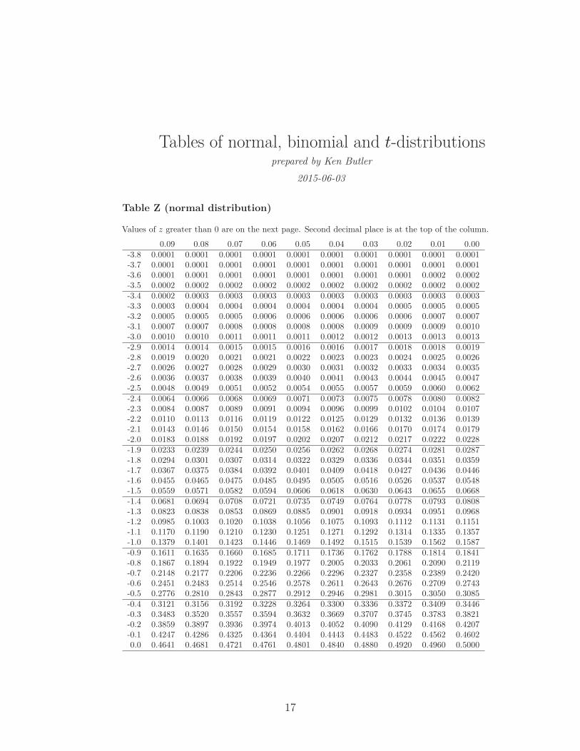
Table Z (normal distribution)
Values of z greater than 0 are on the next page. Second decimal place is at the top of the column.
0.09 0.08 0.07 0.06 0.05 0.04 0.03 0.02 0.01 0.00
-3.8 0.0001 0.0001 0.0001 0.0001 0.0001 0.0001 0.0001 0.0001 0.0001 0.0001
-3.7 0.0001 0.0001 0.0001 0.0001 0.0001 0.0001 0.0001 0.0001 0.0001 0.0001
-3.6 0.0001 0.0001 0.0001 0.0001 0.0001 0.0001 0.0001 0.0001 0.0002 0.0002
-3.5 0.0002 0.0002 0.0002 0.0002 0.0002 0.0002 0.0002 0.0002 0.0002 0.0002
-3.4 0.0002 0.0003 0.0003 0.0003 0.0003 0.0003 0.0003 0.0003 0.0003 0.0003
-3.3 0.0003 0.0004 0.0004 0.0004 0.0004 0.0004 0.0004 0.0005 0.0005 0.0005
-3.2 0.0005 0.0005 0.0005 0.0006 0.0006 0.0006 0.0006 0.0006 0.0007 0.0007
-3.1 0.0007 0.0007 0.0008 0.0008 0.0008 0.0008 0.0009 0.0009 0.0009 0.0010
-3.0 0.0010 0.0010 0.0011 0.0011 0.0011 0.0012 0.0012 0.0013 0.0013 0.0013
-2.9 0.0014 0.0014 0.0015 0.0015 0.0016 0.0016 0.0017 0.0018 0.0018 0.0019
-2.8 0.0019 0.0020 0.0021 0.0021 0.0022 0.0023 0.0023 0.0024 0.0025 0.0026
-2.7 0.0026 0.0027 0.0028 0.0029 0.0030 0.0031 0.0032 0.0033 0.0034 0.0035
-2.6 0.0036 0.0037 0.0038 0.0039 0.0040 0.0041 0.0043 0.0044 0.0045 0.0047
-2.5 0.0048 0.0049 0.0051 0.0052 0.0054 0.0055 0.0057 0.0059 0.0060 0.0062
-2.4 0.0064 0.0066 0.0068 0.0069 0.0071 0.0073 0.0075 0.0078 0.0080 0.0082
-2.3 0.0084 0.0087 0.0089 0.0091 0.0094 0.0096 0.0099 0.0102 0.0104 0.0107
-2.2 0.0110 0.0113 0.0116 0.0119 0.0122 0.0125 0.0129 0.0132 0.0136 0.0139
-2.1 0.0143 0.0146 0.0150 0.0154 0.0158 0.0162 0.0166 0.0170 0.0174 0.0179
-2.0 0.0183 0.0188 0.0192 0.0197 0.0202 0.0207 0.0212 0.0217 0.0222 0.0228
-1.9 0.0233 0.0239 0.0244 0.0250 0.0256 0.0262 0.0268 0.0274 0.0281 0.0287
-1.8 0.0294 0.0301 0.0307 0.0314 0.0322 0.0329 0.0336 0.0344 0.0351 0.0359
-1.7 0.0367 0.0375 0.0384 0.0392 0.0401 0.0409 0.0418 0.0427 0.0436 0.0446
-1.6 0.0455 0.0465 0.0475 0.0485 0.0495 0.0505 0.0516 0.0526 0.0537 0.0548
-1.5 0.0559 0.0571 0.0582 0.0594 0.0606 0.0618 0.0630 0.0643 0.0655 0.0668
-1.4 0.0681 0.0694 0.0708 0.0721 0.0735 0.0749 0.0764 0.0778 0.0793 0.0808
-1.3 0.0823 0.0838 0.0853 0.0869 0.0885 0.0901 0.0918 0.0934 0.0951 0.0968
-1.2 0.0985 0.1003 0.1020 0.1038 0.1056 0.1075 0.1093 0.1112 0.1131 0.1151
-1.1 0.1170 0.1190 0.1210 0.1230 0.1251 0.1271 0.1292 0.1314 0.1335 0.1357
-1.0 0.1379 0.1401 0.1423 0.1446 0.1469 0.1492 0.1515 0.1539 0.1562 0.1587
-0.9 0.1611 0.1635 0.1660 0.1685 0.1711 0.1736 0.1762 0.1788 0.1814 0.1841
-0.8 0.1867 0.1894 0.1922 0.1949 0.1977 0.2005 0.2033 0.2061 0.2090 0.2119
-0.7 0.2148 0.2177 0.2206 0.2236 0.2266 0.2296 0.2327 0.2358 0.2389 0.2420
-0.6 0.2451 0.2483 0.2514 0.2546 0.2578 0.2611 0.2643 0.2676 0.2709 0.2743
-0.5 0.2776 0.2810 0.2843 0.2877 0.2912 0.2946 0.2981 0.3015 0.3050 0.3085
-0.4 0.3121 0.3156 0.3192 0.3228 0.3264 0.3300 0.3336 0.3372 0.3409 0.3446
-0.3 0.3483 0.3520 0.3557 0.3594 0.3632 0.3669 0.3707 0.3745 0.3783 0.3821
-0.2 0.3859 0.3897 0.3936 0.3974 0.4013 0.4052 0.4090 0.4129 0.4168 0.4207
-0.1 0.4247 0.4286 0.4325 0.4364 0.4404 0.4443 0.4483 0.4522 0.4562 0.4602
0.0 0.4641 0.4681 0.4721 0.4761 0.4801 0.4840 0.4880 0.4920 0.4960 0.5000
17

Table Z (continued)
0.00 0.01 0.02 0.03 0.04 0.05 0.06 0.07 0.08 0.09
0.0 0.5000 0.5040 0.5080 0.5120 0.5160 0.5199 0.5239 0.5279 0.5319 0.5359
0.1 0.5398 0.5438 0.5478 0.5517 0.5557 0.5596 0.5636 0.5675 0.5714 0.5753
0.2 0.5793 0.5832 0.5871 0.5910 0.5948 0.5987 0.6026 0.6064 0.6103 0.6141
0.3 0.6179 0.6217 0.6255 0.6293 0.6331 0.6368 0.6406 0.6443 0.6480 0.6517
0.4 0.6554 0.6591 0.6628 0.6664 0.6700 0.6736 0.6772 0.6808 0.6844 0.6879
0.5 0.6915 0.6950 0.6985 0.7019 0.7054 0.7088 0.7123 0.7157 0.7190 0.7224
0.6 0.7257 0.7291 0.7324 0.7357 0.7389 0.7422 0.7454 0.7486 0.7517 0.7549
0.7 0.7580 0.7611 0.7642 0.7673 0.7704 0.7734 0.7764 0.7794 0.7823 0.7852
0.8 0.7881 0.7910 0.7939 0.7967 0.7995 0.8023 0.8051 0.8078 0.8106 0.8133
0.9 0.8159 0.8186 0.8212 0.8238 0.8264 0.8289 0.8315 0.8340 0.8365 0.8389
1.0 0.8413 0.8438 0.8461 0.8485 0.8508 0.8531 0.8554 0.8577 0.8599 0.8621
1.1 0.8643 0.8665 0.8686 0.8708 0.8729 0.8749 0.8770 0.8790 0.8810 0.8830
1.2 0.8849 0.8869 0.8888 0.8907 0.8925 0.8944 0.8962 0.8980 0.8997 0.9015
1.3 0.9032 0.9049 0.9066 0.9082 0.9099 0.9115 0.9131 0.9147 0.9162 0.9177
1.4 0.9192 0.9207 0.9222 0.9236 0.9251 0.9265 0.9279 0.9292 0.9306 0.9319
1.5 0.9332 0.9345 0.9357 0.9370 0.9382 0.9394 0.9406 0.9418 0.9429 0.9441
1.6 0.9452 0.9463 0.9474 0.9484 0.9495 0.9505 0.9515 0.9525 0.9535 0.9545
1.7 0.9554 0.9564 0.9573 0.9582 0.9591 0.9599 0.9608 0.9616 0.9625 0.9633
1.8 0.9641 0.9649 0.9656 0.9664 0.9671 0.9678 0.9686 0.9693 0.9699 0.9706
1.9 0.9713 0.9719 0.9726 0.9732 0.9738 0.9744 0.9750 0.9756 0.9761 0.9767
2.0 0.9772 0.9778 0.9783 0.9788 0.9793 0.9798 0.9803 0.9808 0.9812 0.9817
2.1 0.9821 0.9826 0.9830 0.9834 0.9838 0.9842 0.9846 0.9850 0.9854 0.9857
2.2 0.9861 0.9864 0.9868 0.9871 0.9875 0.9878 0.9881 0.9884 0.9887 0.9890
2.3 0.9893 0.9896 0.9898 0.9901 0.9904 0.9906 0.9909 0.9911 0.9913 0.9916
2.4 0.9918 0.9920 0.9922 0.9925 0.9927 0.9929 0.9931 0.9932 0.9934 0.9936
2.5 0.9938 0.9940 0.9941 0.9943 0.9945 0.9946 0.9948 0.9949 0.9951 0.9952
2.6 0.9953 0.9955 0.9956 0.9957 0.9959 0.9960 0.9961 0.9962 0.9963 0.9964
2.7 0.9965 0.9966 0.9967 0.9968 0.9969 0.9970 0.9971 0.9972 0.9973 0.9974
2.8 0.9974 0.9975 0.9976 0.9977 0.9977 0.9978 0.9979 0.9979 0.9980 0.9981
2.9 0.9981 0.9982 0.9982 0.9983 0.9984 0.9984 0.9985 0.9985 0.9986 0.9986
3.0 0.9987 0.9987 0.9987 0.9988 0.9988 0.9989 0.9989 0.9989 0.9990 0.9990
3.1 0.9990 0.9991 0.9991 0.9991 0.9992 0.9992 0.9992 0.9992 0.9993 0.9993
3.2 0.9993 0.9993 0.9994 0.9994 0.9994 0.9994 0.9994 0.9995 0.9995 0.9995
3.3 0.9995 0.9995 0.9995 0.9996 0.9996 0.9996 0.9996 0.9996 0.9996 0.9997
3.4 0.9997 0.9997 0.9997 0.9997 0.9997 0.9997 0.9997 0.9997 0.9997 0.9998
3.5 0.9998 0.9998 0.9998 0.9998 0.9998 0.9998 0.9998 0.9998 0.9998 0.9998
3.6 0.9998 0.9998 0.9999 0.9999 0.9999 0.9999 0.9999 0.9999 0.9999 0.9999
3.7 0.9999 0.9999 0.9999 0.9999 0.9999 0.9999 0.9999 0.9999 0.9999 0.9999
3.8 0.9999 0.9999 0.9999 0.9999 0.9999 0.9999 0.9999 0.9999 0.9999 0.9999
18
UNIVERSITY OF TORONTO SCARBOROUGH
Department of Computer and Mathematical Sciences
Midterm Test February 2016
STAB22H3 Statistics I, LEC 01 and LEC 02Duration: 1 hour and 45 minutes
Last Name: First Name:
Student number:
Aids allowed:
- One handwritten letter-sized sheet (both sides) of notes prepared by you
- Non-programmable, non-communicating calculator
Standard normal distribution tables are attached at the end.
This test is based on multiple-choice questions. There are 35 questions. All questions carryequal weight. On the Scantron answer sheet, ensure that you enter your last name, firstname (as much of it as fits), and student number (in “Identification”).
Mark in each case the best answer out of the alternatives given (which means the nu-
merically closest answer if the answer is a number and the answer you obtained
is not given.)
Also before you begin, complete the signature sheet, but sign it only when the invigilatorcollects it. The signature sheet shows that you were present at the exam.
There are 18 pages including this page and statistical tables. Please check to see you haveall the pages.
Good luck!!
Answer Key for Exam B
1

1. Three statistics classes (50 students each) took the same test. Shown below are his-tograms of the scores for the classes. Use the histograms to answer the question.
Which class had the highest median score?
(a) Class 1
(b) Class 2
(c) Class 1 and Class 3
(d) Class 3
(e) None, because the classes had the same mean.
2
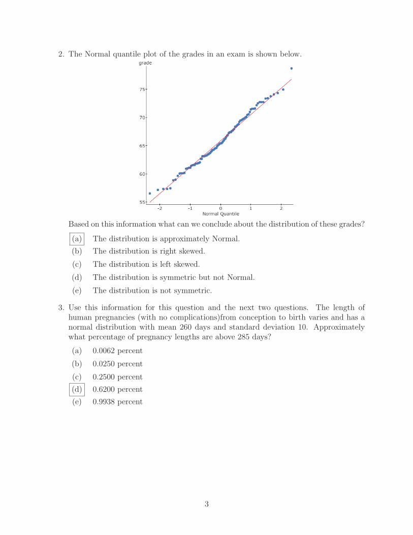
2. The Normal quantile plot of the grades in an exam is shown below.
Based on this information what can we conclude about the distribution of these grades?
(a) The distribution is approximately Normal.
(b) The distribution is right skewed.
(c) The distribution is left skewed.
(d) The distribution is symmetric but not Normal.
(e) The distribution is not symmetric.
3. Use this information for this question and the next two questions. The length ofhuman pregnancies (with no complications)from conception to birth varies and has anormal distribution with mean 260 days and standard deviation 10. Approximatelywhat percentage of pregnancy lengths are above 285 days?
(a) 0.0062 percent
(b) 0.0250 percent
(c) 0.2500 percent
(d) 0.6200 percent
(e) 0.9938 percent
3

4. Refer to the information in question 3 above. The longest five percent of the pregnancylengths are, approximately, longer than what value?
(a) 244
(b) 255
(c) 265
(d) 273
(e) 276
5. Refer to the information in question 3 above. Using 68-95-99.7 rule, what percentageof pregnancy lengths are, approximately, between 250 and 280 days?
(a) 68.0
(b) 81.5
(c) 95
(d) 97.5
(e) 99.7
6. If the correlation coefficient (r)= 1.00, then
(a) all the points on the scatter diagram must fall exactly on a straight line with anegative slope.
(b) all the points on the scatter diagram must fall exactly on a straight line with a
positive slope.
(c) all the points on the scatter diagram must fall exactly on a straight line with azero slope.
(d) all the points on the scatter diagram must fall exactly on a straight line withslope equal to 1.
(e) all the points on the scatter diagram must fall close to a straight line but notnecessarily exactly on straight line.
4

7. Use this information for this question and the next three questions. A survey wasconducted to evaluate the effectiveness of a new flu vaccine that had been administratedin a small community. The vaccine was provided free of charge in a two-shot sequenceover a period of 2 weeks. Some people received the two-shot sequence, some appearedfor only the first shot, and others received neither. A survey of 1000 local residents inthe following spring provided the information shown in the table below. The researcherworking on this data was interested to investigate if this vaccine was successful inreducing the number of flu cases in the community.
TreatmentCases of Flu No Vaccine One shot Two shots Total
Flu 24 9 13 46No flu 289 100 565 954Total 313 109 578 1000
Suppose the researcher wants to compare the proportion of residents who had the fluin the following spring among those who received the two-shot sequences, only thefirst shot, and others that received neither. Which percentage should the researchercalculate?
(a) Row percentage
(b) Column percentage
(c) Joint percentage
(d) Marginal percentage
(e) Marginal percentage of those who did not get the flu
8. In the study in question 7 above, what is the dependent variable?
(a) Treatment
(b) The residents
(c) The researcher
(d) Whether the residents had the flu or not in the following spring
(e) The effect of no vaccine
9. Refer to the information in question 7 above. What percentage of the residents thatreceived no vaccine had the flu in the following spring?
(a) 4.6
(b) 7.7
(c) 24.0
(d) 31.3
(e) 52.2
5

10. Refer to the information in question 7 above. Among those residents who receivedeither one shot or two shots, what is the conditional percentage of those who had theflu in the following spring?
(a) 2.2
(b) 3.2
(c) 10.5
(d) 47.8
(e) 68.7
11. The survey of Teachers Attitude Toward Computers asked teachers to indicate theirfeelings about working with computers as Strongly Disagree, Disagree, Undecided,Agree, or Strongly Agree. What type of a variable is this?
(a) A categorical variable measured on a nominal scale.
(b) A quantitative variable measured on an interval scale
(c) A categorical variable measured on an ordinal scale.
(d) A quantitative variable measured on a nominal scale
(e) A categorical variable measured on an interval scale.
12. Which of the following statements about the Normal density curves is/are true?
I) The total area under the Normal density curve (and above the horizontal line(i.e. density = 0 line ) ) is 1.
II) All Normal density curves are bell-shaped.
III) All bell-shaped density curves are Normal density curves.
(a) Only statement I is true.
(b) Only statements I and II are true.
(c) Only statements II and III are true.
(d) Only statements I and III are true.
(e) All statements I, II and III are true.
13. The distribution for starting salaries in Major League Baseball is highly skewed witha tail to the right.If the median starting income is $500,000 per year, what can be saidabout the mean starting income?
(a) It is less than $500,000 per year.
(b) It is equal to $500,000 per year.
(c) It is greater than $500,000 per year.
(d) It cannot be determined with the given information.
(e) It is equal to the mode.
6

14. The boxplot of the age (in years) at death of a group of 200 individuals is shown below.
Based in this information, what is the interquartile range of the distribution of the ageat death?
(a) 25 years
(b) 30 years
(c) 55 years
(d) 75 years
(e) 85 years
15. Refer to the information in question 14 above. Based on this information how many
individuals in this sample died before the age of 55 years?Note: In order to avoid complications, you may assume that no one in this sample diedexactly at any of the quartiles.
(a) 50 individuals
(b) 55 individuals
(c) 75 individuals
(d) 80 individuals
(e) 85 individuals
7
16. Refer to the information in question 14 above. Based on this information what can wesay about the shape of the distribution of age at death of these individuals.
(a) The distribution of age at death of these individuals is right skewed.
(b) The distribution of age at death of these individuals is left skewed.
(c) The distribution of age at death of these individuals is symmetric.
(d) The distribution of age at death of these individuals is bell-shaped.
(e) This boxplot gives no information about the shape of the distribution.
17. A study investigated the relationship between GPA scores and MCAT scores (scoreson Medical College Admission Test) for 55 applicants who applied to various medicalschools. The study aimed at predicting MCAT scores (y) from GPA scores (x). Assumethat the scatterplot of y against x is approximately linear.The regression equation is: y = 3.92 + 9.10x.For an applicant in this study, the GPA score is 3.62 and the MCAT score is 38. Whatis the residual for this observation?
(a) 1.14
(b) -1.14
(c) 5.06
(d) -5.06
(e) 346.10
18. A researcher wants to construct the regression equation for predicting grocery bills(BILLS) from number of people in the household (NUMBER). He has calculated theslope to be 33.57. The mean BILL is $132.71 and the mean NUMBER is 2.71. Whatis the value of the y-intercept?
(a) 132.71
(b) 8.2
(c) 41.73
(d) 223.68
(e) 130
19. A social researcher collects the following data from 100 residents in a community. Whatvariable is categorical?
(a) Age (in years)
(b) Level of education
(c) Household income
(d) Years of education
(e) Number of children
8

20. Which of the following statements about correlation and regression is/are true?
I) Correlation based on data that are summary statistics are usually higher.
II) If r2 = 0.95, then the response variable increases as the explanatory variableincreases.
III) An outlier always decreases the correlation.
(a) Only statement I is true.
(b) Only statements I and II are true.
(c) Only statements II and III are true.
(d) Only statements I and III are true.
(e) All statements I, II and III are true.
21. The gross revenue (in millions of dollars) for the top 20 movies over the 2001 LaborDay Weekend had median 3.85, the first quartile 1.5, and the third quartile 8.4. Thefour lowest observations had gross revenues 1.2, 1.3, 1.7, 1.8, and the three highestobservations had gross revenues 11, 11.7, 15.8. Based on the 1.5 × IQR rule, howmany outliers are there in this data set of gross revenues?
(a) No outliers
(b) Only one outlier
(c) Only two outliers
(d) Only three outliers
(e) More than three outliers
9

22. Twenty-six households were polled in a marketing survey. The graph below shows thenumber of quarts of milk purchased during a particular week.
Variable: Quarts of milk
Decimal point is at the colon.
Leaf unit = 0.1
0 : 00
0 :
1 : 00000
1 :
2 : 000000000
2 :
3 : 00000
3 :
4 : 000
4 :
5 :
5 :
6 : 00
What percentage of households purchased less than 4 quarts of milk during a particularweek?
(a) 12
(b) 21
(c) 24
(d) 81
(e) 92
23. Refer to the information in question 22 above. What is the shape of the distributionof number of quarts of milk purchased during a particular week?
(a) Exactly symmetrical
(b) Right Skewed
(c) Normal
(d) Bell-shaped
(e) Left skewed
10
24. Refer to the information in question 22 above. What is the most appropriate measureof spread for the data on the number of quarts of milk purchased during a particularweek?
(a) Mode
(b) Standard deviation
(c) Variance
(d) Range
(e) Inter Quartile Range
25. Which of the following statements regarding the standard deviation is FALSE?
(a) The numbers 7, 7, 7 have a standard deviation of 0.
(b) The numbers 8, 9, 10 have a smaller standard deviation than 1, 3, 5.
(c) The numbers 1, 2, 4, 5 have a smaller standard deviation than 1, 1, 5, 5.
(d) The numbers 1, 2, 3 have a smaller standard deviation than 2, 4, 6.
(e) The numbers 3, 5, 7 have a smaller standard deviation than 103, 105, 107.
26. In a study, educational researchers were interested in predicting schools AcademyPerformance Index score (y) on the results of the Stanford 9 Achievement test frompercent of students at that school who are considered English Language Learners(x). Scores ranged from 200 to 1000. The researchers took a random sample of eightelementary schools in Riverside County, California, and recorded schools AcademyPerformance Index (API) scores along with the percent of students at that schoolwho are considered English Language Learners (ELL). The scatterplot of y againstx was approximately linear. Use this information for this question and the next fourquestions. The regression equation is: y = 727.22− 2.46x
The estimated coefficient of determination, R2 is 0.79.
Approximately, what is the estimated correlation, r?
(a) 0.40
(b) 0.79
(c) -0.79
(d) 0.89
(e) -0.89
11

27. Refer to the information in question 26. Which of the following statements is anaccurate interpretation of estimated coefficient of determination, R2 = 0.79 in thecontext of this study.
(a) The percent of students at that school who are considered ELL causes APIscores to increase by 0.79%
(b) About 79% of variation in API scores is explained by the linear regression with
the percent of students at that school who are considered ELL.
(c) About 79% of API scores is explained by the linear regression with the percentof students at that school who are considered ELL.
(d) About 79% of variation in the percent of students who are considered ELL inthese schools is explained by the linear regression with API scores.
(e) About 79% of the percent of students who are considered ELL in these schoolsis explained by the linear regression with API scores.
28. Refer to the information in question 26. The slope of the regression line is -2.46. Thismeans that:
(a) When the percentage of students who are considered ELL increases by 1, the
mean API score is estimated to decrease by 2.46.
(b) When the percentage of students who are considered ELL increases by 1, themean API score is estimated to increase by 2.46.
(c) When the API score increases by 1, the mean percentage of students who areconsidered ELL is estimated to increase by 2.46.
(d) When the API score increases by 1, the mean percentage of students who areconsidered ELL is estimated to decrease by 2.46.
(e) The estimated mean API score is -2.46.
29. Refer to the information in question 26. If x = 0 was in the observed range of x values,which of the following statements is true?
(a) The mean percent of students who are considered ELL is estimated to be 0.
(b) There would be no relationship between API scores and the percent of studentswho are considered ELL.
(c) The mean score in API is estimated to be 727.22 when the percentage of students
who are considered ELL is 0.
(d) There would be no meaningful relationship between API scores and the percentof students who are considered ELL.
(e) The mean score in API is estimated to be 0 when the percentage of studentswho are considered ELL is 0.
12

30. In checking the adequacy of the regression model, the plot below shows that:
(a) Residual points are evenly spread out. No major pattern is seen. Thus, theregression model is correct.
(b) Residual points are evenly spread out. No major pattern is seen. Thus, theregression model is incorrect.
(c) Residual points are not evenly spread out. A major pattern is observed. Thus,the regression model is correct.
(d) Residual points are not evenly spread out. A pattern is observed. Thus, the
regression model is incorrect
(e) As x values increases, residual points increases. Thus, regression model is cor-rect.
31. A student in STAB22 did all ten quizzes. The average of the grades of these ten quizzesis 8.0. According to our quiz evaluation policy, we drop the lowest quiz grade and usethe average of the grades of the best nine quizzes. This student’s lowest quiz grade is3.0. If we drop this lowest quiz, what is the average of the grades of the other ninequizzes? (i.e. the average of her best nine quiz grades)?
(a) 8.0
(b) 8.2
(c) 8.6
(d) 9.0
(e) 9.4
13
32. Which of the following values of the correlation r indicates the strongest correlationbetween the two variables?
(a) r = 1.22
(b) r = −1.90
(c) r = 0.75
(d) r = −0.81
(e) r = 1.22
33. Which of the following statements about influential and/or high leverage points is/aretrue?
I) Removal of an influential point changes the regression line.
II) All high leverage points are influential.
III) All hight leverage points have large residuals.
(a) Only statement I is true.
(b) Only statements I and II are true.
(c) Only statements II and III are true.
(d) Only statements I and III are true.
(e) All statements I, II and III are true.
14

34. The graph below represents the percentage of workers living in 18 Canadian cities whoused public transportation to commute to work.Note: In order to avoid complications, you may assume that no city in this sample hadpercentage of workers who used public transportation exactly at a class boundary.
Based in this information, which of the following statements is true?
(a) More than 30 percent of workers in this sample used public transportation tocommute to work.
(b) About 22 percent of cities in this sample had more than 30 percent of their
workers who used public transportation to commute to work.
(c) About 4 percent of cities in this sample had more than 30 percent of theirworkers who used public transportation to commute to work
(d) More than 30 percent of cities in this sample had workers who used public
transportation to commute to work.
(e) About 3 percent of cities in this sample had more than 30 percent of theirworkers who used public transportation to commute to work.
15

35. The stemplot below shows the annual family incomes (in dollars) of a random sampleof 20 families selected from a city.
Variable: Family Income
Decimal point is 5 digit(s) to the right of the colon.
Leaf unit = 10000
0 : 11222333
0 : 55788899
1 : 022
1 : 7
Use this data to calculate the third quartile (Q3)of the family income.
(a) 20000 dollars
(b) 50000 dollars
(c) 9000 dollars
(d) 5000 dollars
(e) 90000 dollars
16

Tables of normal, binomial and t-distributionsprepared by Ken Butler
2015-06-03
Table Z (normal distribution)
Values of z greater than 0 are on the next page. Second decimal place is at the top of the column.
0.09 0.08 0.07 0.06 0.05 0.04 0.03 0.02 0.01 0.00
-3.8 0.0001 0.0001 0.0001 0.0001 0.0001 0.0001 0.0001 0.0001 0.0001 0.0001
-3.7 0.0001 0.0001 0.0001 0.0001 0.0001 0.0001 0.0001 0.0001 0.0001 0.0001
-3.6 0.0001 0.0001 0.0001 0.0001 0.0001 0.0001 0.0001 0.0001 0.0002 0.0002
-3.5 0.0002 0.0002 0.0002 0.0002 0.0002 0.0002 0.0002 0.0002 0.0002 0.0002
-3.4 0.0002 0.0003 0.0003 0.0003 0.0003 0.0003 0.0003 0.0003 0.0003 0.0003
-3.3 0.0003 0.0004 0.0004 0.0004 0.0004 0.0004 0.0004 0.0005 0.0005 0.0005
-3.2 0.0005 0.0005 0.0005 0.0006 0.0006 0.0006 0.0006 0.0006 0.0007 0.0007
-3.1 0.0007 0.0007 0.0008 0.0008 0.0008 0.0008 0.0009 0.0009 0.0009 0.0010
-3.0 0.0010 0.0010 0.0011 0.0011 0.0011 0.0012 0.0012 0.0013 0.0013 0.0013
-2.9 0.0014 0.0014 0.0015 0.0015 0.0016 0.0016 0.0017 0.0018 0.0018 0.0019
-2.8 0.0019 0.0020 0.0021 0.0021 0.0022 0.0023 0.0023 0.0024 0.0025 0.0026
-2.7 0.0026 0.0027 0.0028 0.0029 0.0030 0.0031 0.0032 0.0033 0.0034 0.0035
-2.6 0.0036 0.0037 0.0038 0.0039 0.0040 0.0041 0.0043 0.0044 0.0045 0.0047
-2.5 0.0048 0.0049 0.0051 0.0052 0.0054 0.0055 0.0057 0.0059 0.0060 0.0062
-2.4 0.0064 0.0066 0.0068 0.0069 0.0071 0.0073 0.0075 0.0078 0.0080 0.0082
-2.3 0.0084 0.0087 0.0089 0.0091 0.0094 0.0096 0.0099 0.0102 0.0104 0.0107
-2.2 0.0110 0.0113 0.0116 0.0119 0.0122 0.0125 0.0129 0.0132 0.0136 0.0139
-2.1 0.0143 0.0146 0.0150 0.0154 0.0158 0.0162 0.0166 0.0170 0.0174 0.0179
-2.0 0.0183 0.0188 0.0192 0.0197 0.0202 0.0207 0.0212 0.0217 0.0222 0.0228
-1.9 0.0233 0.0239 0.0244 0.0250 0.0256 0.0262 0.0268 0.0274 0.0281 0.0287
-1.8 0.0294 0.0301 0.0307 0.0314 0.0322 0.0329 0.0336 0.0344 0.0351 0.0359
-1.7 0.0367 0.0375 0.0384 0.0392 0.0401 0.0409 0.0418 0.0427 0.0436 0.0446
-1.6 0.0455 0.0465 0.0475 0.0485 0.0495 0.0505 0.0516 0.0526 0.0537 0.0548
-1.5 0.0559 0.0571 0.0582 0.0594 0.0606 0.0618 0.0630 0.0643 0.0655 0.0668
-1.4 0.0681 0.0694 0.0708 0.0721 0.0735 0.0749 0.0764 0.0778 0.0793 0.0808
-1.3 0.0823 0.0838 0.0853 0.0869 0.0885 0.0901 0.0918 0.0934 0.0951 0.0968
-1.2 0.0985 0.1003 0.1020 0.1038 0.1056 0.1075 0.1093 0.1112 0.1131 0.1151
-1.1 0.1170 0.1190 0.1210 0.1230 0.1251 0.1271 0.1292 0.1314 0.1335 0.1357
-1.0 0.1379 0.1401 0.1423 0.1446 0.1469 0.1492 0.1515 0.1539 0.1562 0.1587
-0.9 0.1611 0.1635 0.1660 0.1685 0.1711 0.1736 0.1762 0.1788 0.1814 0.1841
-0.8 0.1867 0.1894 0.1922 0.1949 0.1977 0.2005 0.2033 0.2061 0.2090 0.2119
-0.7 0.2148 0.2177 0.2206 0.2236 0.2266 0.2296 0.2327 0.2358 0.2389 0.2420
-0.6 0.2451 0.2483 0.2514 0.2546 0.2578 0.2611 0.2643 0.2676 0.2709 0.2743
-0.5 0.2776 0.2810 0.2843 0.2877 0.2912 0.2946 0.2981 0.3015 0.3050 0.3085
-0.4 0.3121 0.3156 0.3192 0.3228 0.3264 0.3300 0.3336 0.3372 0.3409 0.3446
-0.3 0.3483 0.3520 0.3557 0.3594 0.3632 0.3669 0.3707 0.3745 0.3783 0.3821
-0.2 0.3859 0.3897 0.3936 0.3974 0.4013 0.4052 0.4090 0.4129 0.4168 0.4207
-0.1 0.4247 0.4286 0.4325 0.4364 0.4404 0.4443 0.4483 0.4522 0.4562 0.4602
0.0 0.4641 0.4681 0.4721 0.4761 0.4801 0.4840 0.4880 0.4920 0.4960 0.5000
17

Table Z (continued)
0.00 0.01 0.02 0.03 0.04 0.05 0.06 0.07 0.08 0.09
0.0 0.5000 0.5040 0.5080 0.5120 0.5160 0.5199 0.5239 0.5279 0.5319 0.5359
0.1 0.5398 0.5438 0.5478 0.5517 0.5557 0.5596 0.5636 0.5675 0.5714 0.5753
0.2 0.5793 0.5832 0.5871 0.5910 0.5948 0.5987 0.6026 0.6064 0.6103 0.6141
0.3 0.6179 0.6217 0.6255 0.6293 0.6331 0.6368 0.6406 0.6443 0.6480 0.6517
0.4 0.6554 0.6591 0.6628 0.6664 0.6700 0.6736 0.6772 0.6808 0.6844 0.6879
0.5 0.6915 0.6950 0.6985 0.7019 0.7054 0.7088 0.7123 0.7157 0.7190 0.7224
0.6 0.7257 0.7291 0.7324 0.7357 0.7389 0.7422 0.7454 0.7486 0.7517 0.7549
0.7 0.7580 0.7611 0.7642 0.7673 0.7704 0.7734 0.7764 0.7794 0.7823 0.7852
0.8 0.7881 0.7910 0.7939 0.7967 0.7995 0.8023 0.8051 0.8078 0.8106 0.8133
0.9 0.8159 0.8186 0.8212 0.8238 0.8264 0.8289 0.8315 0.8340 0.8365 0.8389
1.0 0.8413 0.8438 0.8461 0.8485 0.8508 0.8531 0.8554 0.8577 0.8599 0.8621
1.1 0.8643 0.8665 0.8686 0.8708 0.8729 0.8749 0.8770 0.8790 0.8810 0.8830
1.2 0.8849 0.8869 0.8888 0.8907 0.8925 0.8944 0.8962 0.8980 0.8997 0.9015
1.3 0.9032 0.9049 0.9066 0.9082 0.9099 0.9115 0.9131 0.9147 0.9162 0.9177
1.4 0.9192 0.9207 0.9222 0.9236 0.9251 0.9265 0.9279 0.9292 0.9306 0.9319
1.5 0.9332 0.9345 0.9357 0.9370 0.9382 0.9394 0.9406 0.9418 0.9429 0.9441
1.6 0.9452 0.9463 0.9474 0.9484 0.9495 0.9505 0.9515 0.9525 0.9535 0.9545
1.7 0.9554 0.9564 0.9573 0.9582 0.9591 0.9599 0.9608 0.9616 0.9625 0.9633
1.8 0.9641 0.9649 0.9656 0.9664 0.9671 0.9678 0.9686 0.9693 0.9699 0.9706
1.9 0.9713 0.9719 0.9726 0.9732 0.9738 0.9744 0.9750 0.9756 0.9761 0.9767
2.0 0.9772 0.9778 0.9783 0.9788 0.9793 0.9798 0.9803 0.9808 0.9812 0.9817
2.1 0.9821 0.9826 0.9830 0.9834 0.9838 0.9842 0.9846 0.9850 0.9854 0.9857
2.2 0.9861 0.9864 0.9868 0.9871 0.9875 0.9878 0.9881 0.9884 0.9887 0.9890
2.3 0.9893 0.9896 0.9898 0.9901 0.9904 0.9906 0.9909 0.9911 0.9913 0.9916
2.4 0.9918 0.9920 0.9922 0.9925 0.9927 0.9929 0.9931 0.9932 0.9934 0.9936
2.5 0.9938 0.9940 0.9941 0.9943 0.9945 0.9946 0.9948 0.9949 0.9951 0.9952
2.6 0.9953 0.9955 0.9956 0.9957 0.9959 0.9960 0.9961 0.9962 0.9963 0.9964
2.7 0.9965 0.9966 0.9967 0.9968 0.9969 0.9970 0.9971 0.9972 0.9973 0.9974
2.8 0.9974 0.9975 0.9976 0.9977 0.9977 0.9978 0.9979 0.9979 0.9980 0.9981
2.9 0.9981 0.9982 0.9982 0.9983 0.9984 0.9984 0.9985 0.9985 0.9986 0.9986
3.0 0.9987 0.9987 0.9987 0.9988 0.9988 0.9989 0.9989 0.9989 0.9990 0.9990
3.1 0.9990 0.9991 0.9991 0.9991 0.9992 0.9992 0.9992 0.9992 0.9993 0.9993
3.2 0.9993 0.9993 0.9994 0.9994 0.9994 0.9994 0.9994 0.9995 0.9995 0.9995
3.3 0.9995 0.9995 0.9995 0.9996 0.9996 0.9996 0.9996 0.9996 0.9996 0.9997
3.4 0.9997 0.9997 0.9997 0.9997 0.9997 0.9997 0.9997 0.9997 0.9997 0.9998
3.5 0.9998 0.9998 0.9998 0.9998 0.9998 0.9998 0.9998 0.9998 0.9998 0.9998
3.6 0.9998 0.9998 0.9999 0.9999 0.9999 0.9999 0.9999 0.9999 0.9999 0.9999
3.7 0.9999 0.9999 0.9999 0.9999 0.9999 0.9999 0.9999 0.9999 0.9999 0.9999
3.8 0.9999 0.9999 0.9999 0.9999 0.9999 0.9999 0.9999 0.9999 0.9999 0.9999
18