UNIVERSITY OF TORONTO SCARBOROUGHDepartment of Computer and Mathematical Sciences

Sample Midterm Test

STAC67H3 Regression AnalysisDuration: One hour and fifty minutes

Last Name: First Name:

Student number:

Aids allowed:

- The textbook: Applied Regression Analysis by Ketner et al published by McGraw Hill

- Class notes

- A calculator (No phone calculators are allowed)

No other aids are allowed. For example you are not allowed to have any other textbook orpast exams.

All your work must be presented clearly in order to get credit. Answer alone (even thoughcorrect) will only qualify for ZERO credit. Please show your work in the space provided;you may use the back of the pages, if necessary, but you MUST remain organized. Show yourwork and answer in the space provided, in ink. Pencil may be used, but then any re-gradingwill NOT be allowed.

There are 14 pages including this page. Please check to see you have all the pages.

Good Luck!

Question: 1 2 3 4 Total

Points: 19 20 10 11 60

Score:

Page 2 of 14

1. The following data ( and the summary statistics) relate biomass production of soybeansto cumulative intercepted solar radiation over an eight-week period following emergence.Biomass production is the mean dry weight in grams of independent samples of fourplants (Virginia Lesser and Mike Unsworth).

Row SolarRadiation(x) PlantBiomass(y)

1 29.7 16.6

2 68.4 49.1

3 120.7 121.7

4 217.2 219.6

5 313.5 375.5

6 419.1 570.8

7 535.9 648.2

8 641.5 755.6∑x = 2346,

∑y = 2757,

∑x2 = 1039943.1,

∑y2 = 1523629,

∑xy = 1255267

Assume that the data satisfied the necessary assumptions for the tests and confidenceintervals below.

(a) (6 points) Calculate b0 and b1 for the linear regression of plant biomass(y) on in-tercepted solar radiation(x).

Solution: b1 = SSXY

SSXX=

1255267− 2346×27578

1039943.1− 23462

8

= 1.27.

b0 = y − b1x = 27578− 1.27× 2346

8= −27.8

(b) (6 points) Calculate a 95% confidence interval for β1.

Solution: SSTot = 1523629− 27572

8= 573497.875, SSReg = b2

1SSXX = 1.272×(1039943− 23462

8) ≈ 567706, SSE = SSTot− SSReg ≈ 573497.875− 567706 ≈

5791.875, s =√MSE =

√5791.9/6 ≈ 31, sb1 = s√

SSXX= 31√

1039943.1− 23462

8

≈

0.05 and the CI is b1 ± t0.975,6sb1 = 1.27± 2.4469× 0.05.

(c) (3 points) Test the null hypothesis H0 : β1 = 1 against the alternative H1 : β1 6= 1.

Solution: t = b1−1sb1

= 1.27−10.05

= 5.4 and the p-value < 0.05 and so reject H0 :

β1 = 1 in favour of the alternative H1 : β1 6= 1. (Or just see that 1 /∈ CI in partb above).

(d) (4 points) Calculate the 95% confidence interval estimates of the mean biomassproduction for X = 300.

Question 1 continues on the next page. . .

Page 3 of 14

Solution: SSXX = 1039943.1 − 23462

8= 351978. The predicted value y =

−27.8 + 1.27 × 300 = 353.4 and the CI for the mean at x = 300 is = y ±

tn−2,α/2s√

1n

+ (xh−x)2

SSXX= 353.4± 2.4469× 31×

√18

+(300− 2346

8 )2

351978.

Question 1 continues on the next page. . .

Page 4 of 14

You may continue your to answer to question 1 on this page

Page 5 of 14

2. (Samuel, M. et. al.) Laetisaric acid is a compound that holds promise for control offungus diseases in crop plants. The accompanying data show the results of growing thefungus Pythium ultimum in various concentrations(in µG/ml) of laetisaric acid. Eachgrowth value is the average of four radial measurements(mm) of a colony grown in apetri dish for 24 hours. Some R outputs (with codes) from the analysis of the data fromthis study based on the Normal error regression model are given below:

> fungus=read.table("C:/Users/Mahinda/Desktop/fungus.txt", header=T)

> fungus

Row AcidConc Growth

1 1 0 33.3

... only the first and the last observations are printed here

12 12 30 10.0

> Growth <- fungus[,3]

> AcidConc <- fungus[,2]

> plot(AcidConc, Growth)

0 5 10 15 20 25 30

10

15

20

25

30

AcidConc

Gro

wth

> fit = lm(Growth ~AcidConc)

> summary(fit)

Call: lm(formula = Growth ~ AcidConc)

Residuals:

Min 1Q Median 3Q Max

-2.0896 -0.8498 0.2743 0.9004 1.4702

Coefficients:

Estimate Std. Error t value Pr(>|t|)

(Intercept) 31.82979 0.55693 57.15 6.53e-14 ***

AcidConc -0.71201 0.03589 -19.84 2.32e-09 ***

Question 2 continues on the next page. . .

Page 6 of 14

---

Signif. codes: 0 *** 0.001 ** 0.01 * 0.05 . 0.1 1

Residual standard error: 1.295 on 10 degrees of freedom Multiple

R-squared: 0.9752, Adjusted R-squared: 0.9727 F-statistic: 393.6

on 1 and 10 DF, p-value: 2.321e-09

> anova(fit)

Analysis of Variance Table

Response: Growth

Df Sum Sq Mean Sq F value Pr(>F)

AcidConc 1 660.57 660.57 393.64 2.321e-09 ***

Residuals 10 16.78 1.68

---

Signif. codes: 0 *** 0.001 ** 0.01 * 0.05 . 0.1 1

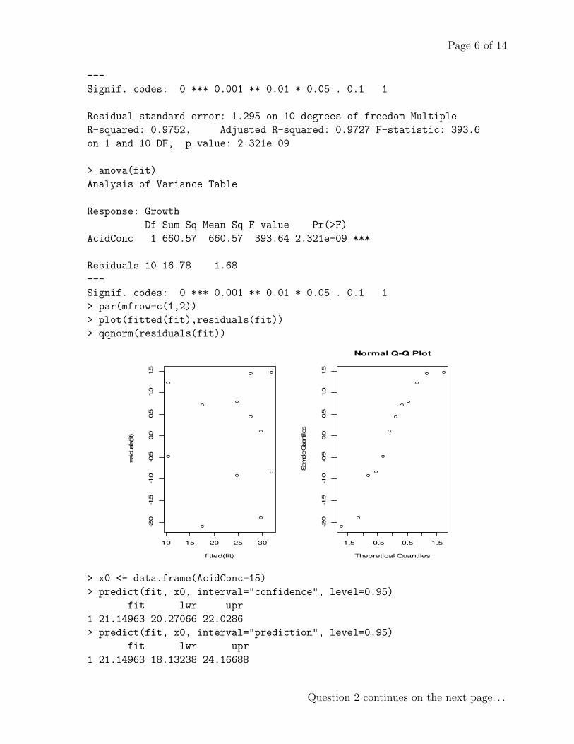
> par(mfrow=c(1,2))

> plot(fitted(fit),residuals(fit))

> qqnorm(residuals(fit))

10 15 20 25 30

-2.0

-1.5

-1.0

-0.5

0.0

0.5

1.0

1.5

fitted(fit)

residuals(fit)

-1.5 -0.5 0.5 1.5

-2.0

-1.5

-1.0

-0.5

0.0

0.5

1.0

1.5

Normal Q-Q Plot

Theoretical Quantiles

Sample Q

uantiles

> x0 <- data.frame(AcidConc=15)

> predict(fit, x0, interval="confidence", level=0.95)

fit lwr upr

1 21.14963 20.27066 22.0286

> predict(fit, x0, interval="prediction", level=0.95)

fit lwr upr

1 21.14963 18.13238 24.16688

Question 2 continues on the next page. . .

Page 7 of 14

(a) (3 points) Describe what you learn from the scatterplot of growth on Acid concen-tration.

Solution: A strong, linear, negative relationship.

(b) (2 points) What proportion of the variability in fungal growth is explained by thisregression linear regression with acid concentration?

Solution: 97.52% (The proportion of the variability in fungal growth is ex-plained by this regression linear regression with acid concentration means R-sq)

(c) (4 points) Comment on the residual plots (i.e the plot of residuals vs fitted valuesand the Normal QQ plot of residuals)

Solution: The plot of residuals vs fitted values looks random. This indicatesthat there is no serious violation of the assumption of independence of errors.The Normal QQ plot is close to s straight line indicating no serious violation ofthe assumption of Normality of errors.

Question 2 continues on the next page. . .

Page 8 of 14

Note: For the remaining parts of this question, assume that the data satisfied allthe necessary assumptions, regardless of your answers to parts a, b and c above.

(d) (3 points) Is there significant evidence (at α = 0.05) for a linear relationship be-tween fungus growth and acid concentration? Give reasons to your answer.

Solution: Yes, the p-value for testing the null hypothesis H0 : β1 = 0 againstthe alternative H1 : β1 6= 0 is less than 0.05 (p-value = 2.32e-09 )

(e) (3 points) Construct a 95% confidence interval for the change in mean fungal growthwhen the acid concentration increases by 1 µG/ml.

Solution: −0.71201± t0.975,10 × 0.03589 = −0.71201± 2.228× 0.03589 (df canbe obtained from the ANOVA table)

(f) (5 points) Calculate a 90% confidence interval for the mean fungal growth whenthe acid concentration is 15 µG/ml.Note This question requires a numerical answer. Just stating whether this intervalis wider or narrower is not an acceptable answer.

Solution: Note that the R output gives the 95% CI for the mean of Y at x =15, and the question wants the 90% CI.y = 21.14963 and t0.975,10 × sy = (22.0286 − 20.27066)/2 = 0.87897 and sosy = 0.87897/2.228 = 0.394510772 and the 90% CI for the mean of Y is y ±

Question 2 continues on the next page. . .

Page 9 of 14

t0.95,10 × sy = 21.14963± 1.812× 0.394510772 = (20.43, 21.86).Here is the R output (just to compare the above calculations)

> predict(fit, x0, interval="confidence", level=0.90)

fit lwr upr

1 21.14963 20.43464 21.86462

Page 10 of 14

3. A simple linear regression was run on a data set with n = 6 observations . You are givenonly the following information:

• The regression equation is y = - 5.36 + 0.0405 x

• The value of the t-test statistic for testing null hypothesis H0 : β1 = 0 against thealternative H1 : β1 6= 0 is 9.25.

• MSE = 2.16

(a) (4 points) Calculate a 95% confidence interval for β1.

Solution: sb1 = 0.0405/9.25 = 0.004378, t(0.975, 6− 2) = 2.776 and so the CIis (0.0405± 2.776× 0.004378) = (0.028, 0.053)

(b) (6 points) Calculate and interpret the coefficient of determination (R2).

Solution: F = MSRegMSE

= t2 = 9.252 =⇒ MSReg = 9.252 × 2.16 = 184.815.SSE = MSE× (n−2) = 2.16×4 = 8.64 and SSReg = MSReg×1 = 184.815,SSTot = SSReg + SSE = 184.815 + 8.64 = 193.455, R2 = SSReg

SSTot= 184.815

193.455=

0.955, i.e. 95.5% of the variability in y is explained by this linear regressionwith x.

Here is a software(MINITAB) output (just to compare the calculated values):

The regression equation is y = - 5.36 + 0.0405 x

Predictor Coef SE Coef T P

Constant -5.360 1.558 -3.44 0.026

x 0.040488 0.004375 9.25 0.001

S = 1.46824 R-Sq = 95.5% R-Sq(adj) = 94.4%

Analysis of Variance

Source DF SS MS F P

Regression 1 184.63 184.63 85.65 0.001

Residual Error 4 8.62 2.16

Total 5 193.26

Question 3 continues on the next page. . .

Page 11 of 14

You may continue your to answer to question 3 on this page

Page 12 of 14

4. Consider the regression model with no intercept given by Yi = βxi + εi, i = 1 . . . n withthe following assumptions:

1. εi’s are independent.

2. E(εi) = 0 for i = 1 . . . n

3. V ar(εi) = σ2 for i = 1 . . . n

4. xi’s are known constants.

Note that εi’s are NOT necessarily Normally distributed and recall that in class we

showed (in an exercise) that B =∑n

i=1 xiYi∑ni=1 x

2i

is the least squares estimator of β and it is

an unbiased estimator of β.

(a) (3 points) Prove that V ar(B) = σ2∑ni=1 x

2i

Solution: V ar(B) =∑n

i=1 x2i V ar(Yi)

(∑n

i=1 x2i )

2 =σ2

∑ni=1 x

2i

(∑n

i=1 x2i )

2 = σ2∑ni=1 x

2i.

(b) (5 points) Prove that E(Yi −Bxi)2 = σ2(

1− x2i∑ni=1 x

2i

)Solution: E(Yi −Bxi)2 = E(Yi − βxi + βxi −Bxi)2 = V ar(Yi) + x2

iV ar(B)−2xiCov(Yi, B) = σ2 +

σ2x2i∑ni=1 x

2i− 2x2i∑n

i=1 x2iV ar(Yi) = σ2− σ2x2i∑n

i=1 x2i

= σ2(

1− x2i∑ni=1 x

2i

).

(c) (3 points) Prove that S2 = 1n−1

∑ni=1(Yi −Bxi)2 is an unbiased estimator of σ2.

Solution: E(S2) = 1n−1

∑ni=1E(Yi−Bxi)2) = 1

n−1

∑ni=1 σ

2(

1− x2i∑ni=1 x

2i

)= σ2.

Question 4 continues on the next page. . .

Page 13 of 14

You may continue your to answer to question 4 on this page

END OF TEST

Page 14 of 14