Embed Size (px)
Citation preview

University of Lusaka, ECF 110: Introduction to Macroeconomics, Prepared by Nchimunya Ndiili Kunda Page 1
UNIVERSITY OF LUSAKA
FACULTY OF ECONOMICS, BUSINESS & MANAGEMENT
UNDERGRADUATES PROGRAM
INTRODUCTION TO MACROECONOMICS
ED:230
COURSE MODULE

University of Lusaka, ECF 110: Introduction to Macroeconomics, Prepared by Nchimunya Ndiili Kunda Page 2
TABLE OF CONTENTS
UNIT 1: MACROECONOMIC OVERVIEW………………………………………………………………………5
Definition of macroeconomics …………………………………………………………………5
Objectives of macroeconomics………………………………………………………………...5
Instruments of macroeconomics……………………………………………………………….6
UNIT 2: MEASUREMENT OF ECONOMIC PERFORMANCE………………………………………………..7
Concepts: GNP,GDP NI and other economic indicators…………………………………..7
GDP concept……………………………………………………………………………7
GNP concept……………………………………………………………………………8
NI concept………………………………………………………………………………9
Other economic indicators……………………………………………………………………...9
Inflation rate…………………………………………………………………………….9
Unemployment rate…………………………………………………………………..10
Expenditure and Income approach…………………………………………………………..11
Income approach……………………………………………………………………..11
Expenditure approach………………………………………………………………..11
National income account computation……………………………………………………….12
Problems in measuring national income…………………………………………………….12
UNIT 3: NATIONAL INCOME…………………………………………………………………………………….13
Aggregate demand and output……………………………………………………………….13
Definition of AD……………………………………………………………………….13
Determinants of AD…………………………………………………………………..13
Aggregate demand curves…………………………………………………………..14
Shifts in AD……………………………………………………………………………15
Aggregate Expenditure model (AE)………………………………………………………...17
Definition of AE model……………………………………………………………….17
Consumption function………………………………………………………………..17
Saving function………………………………………………………………………..18
National income equilibrium…………………………………………………………………..19
Definition of National Income equilibrium………………………………………….19
Adjustments towards equilibrium……………………………………………………19
The Multiplier model……………………………………………………………………………20
Definition of equilibrium………………………………………………………………20
Equilibrium using the multiplier model……………………………………………...20
Paradox of shifts – Savings & Investments………………………………………………….22

University of Lusaka, ECF 110: Introduction to Macroeconomics, Prepared by Nchimunya Ndiili Kunda Page 3
UNIT 4: FISCAL POLICY…………………………………………………………………………………………24
Goals of fiscal policy ………………………………………………………………………….24
Tools of Fiscal policy………………………………………………………………………….24
Government spending………………………………………………………………..24
Taxation………………………………………………………………………………..24
Fiscal policy expansion and contraction……………………………………………………..25
Fiscal policy expansion………………………………………………………………25
Fiscal policy contraction ……………………………………………………………..26
Effects of Governments spending and taxes on output……………………………………26
Crowding out effect…………………………………………………………………………….27
Fiscal Policy and budget deficit……………………………………………………………….28
The national debt and the deficit……………………………………………………………..29
Limitations of Fiscal policy……………………………………………………………………29
UNIT 5: MONETARY POLICY…………………………………………………………………………………...30
Goals of Monetary policy ……………………………………………………………………30
Tools of Monetary policy……………………………………………………………………..30
Discount rate………………………………………………………………………….30
Reserve ratio………………………………………………………………………….30
Open market operations……………………………………………………………..30
Monetary policy expansion and contraction ( IS –LM Model)…………………………….31
UNIT 6: MONEY AND BANKING………………………………………………………………………………..34
Definition and types of money………………………………………………………………...34
Functions of money…………………………………………………………………………….35
The demand for money……………………………………………………………………….36
The supply for money…………………………………………………………………………37
The central bank……………………………………………………………………...37
The functions of the commercial banks……………………………………………38
Creation of money……………………………………………………………………………...39
Multiple deposit expansion…………………………………………………………..39
Money multiplier………………………………………………………………………40
UNIT 7: INFLATION……………………………………………………………………………………………….41
Definitions of inflation………………………………………………………………………….41
Measurement of inflation………………………………………………………………………42
Causes of inflation……………………………………………………………………………..43
Effects of inflation………………………………………………………………………………46
Cures of inflation……………………………………………………………………………….47
UNIT 8: UNEMPLOYMENT……………………………………………………………………………………...52
Defining ‗full‘ employment……………………………………………………………………..52
Types of unemployment……………………………………………………………………….53
Measures of Unemployment………………………………………………………………….54

University of Lusaka, ECF 110: Introduction to Macroeconomics, Prepared by Nchimunya Ndiili Kunda Page 4
Costs of unemployment……………………………………………………………………….55
Economic costs of unemployment…………………………………………………55
Social costs of unemployment……………………………………………………..56
Inflation and unemployment (Phillips curve)………………………………………………57
The original Philips curve…………………………………………………………..57
The critics on the Philips curve…………………………………………………….58
The expected augmented Philips curve…………………………………………..59
UNIT 9: THE OPEN MARKET…………………………………………………………………………………..61
The open Market……………………………………………………………………………….61
International Trade……………………………………………………………………………..62
Basis of trade………………………………………………………………………….63
Terms of trade………………………………………………………………………...67
Trade barriers…………………………………………………………………………68
Trade protection………………………………………………………………………70
Free trade bodies…………………………………………………………………….74
Balance of Payments………………………………………………………………………….74
Components of BOP…………………………………………………………………74
Current account………………………………………………………………………74
Capital account……………………………………………………………………….74
Current account deficit………………………………………………………………74
Zambia balance of payment………………………………………………………..75
Foreign Exchange rates……………………………………………………………………………76
Definition exchange rates………………………………………………………………...76
Types of exchange rates………………………………………………………………….76
Exchange rates regime…………………………………………………………………...79
Effects exchange rates on investments…………………………………………………80
Devaluation…………………………………………………………………………………81
UNIT 10: ECONOMIC GROWTH AND BUSINESS CYCLE………………………………………………….82
Business cycles……………………………………………………………………………82
Definition of Growth……………………………………………………………………….83
Classical growth theory…………………………………………………………83
Neo –classical growth theory…………………………………………………..83
Endogenous growth theory……………………………………………………..84
Factors of growth………………………………………………………………………….84
Bibliography………………………………………………………………………………………………………..87

University of Lusaka, ECF 110: Introduction to Macroeconomics, Prepared by Nchimunya Ndiili Kunda Page 5
UNIT: 1
TOPIC: MACROECONOMICS OVERVIEW
OBJECTIVE:
At the end of the lesson, students must understand macroeconomics as the study of aggregates of the whole
economy. They should clearly differentiate the micro economic and macro economics concepts and relate the
macroeconomic concepts to the economic activities in the world.
SUB- TOPICS:
- Definition of macroeconomics
- Objectives and instruments of macroeconomics
A. Definition of Macroeconomics
- ‗Macroeconomics is the study of the behavior of the economy as a whole.‖ (Samuelson .N, 2007)
- ‗Macroeconomics is the study of aggregate economic variables.‖ ( Blanchard,O, 2007) - Examples of aggregates are aggregate production, average price level, unemployment rate, inflation,
unemployment, and industrial production. The aggregate will be covered in detail in other lectures. - The distinction between Microeconomics and Macroeconomics is that they stress on different issues.
Macroeconomics considers the industrial sector, the services sector or the farm sector but not consider
specific parts of any of these sectors. Microeconomics considers units production and prices in a specific
markets such as unit prices of commodities, individual demand for goods and services.
B. Objectives of macroeconomics
- The objective of Macroeconomics is to explain the behavior of the aggregates variables due to the effect
of government policies. This is achieved by :
Making assumptions to simplify the analysis
Construct simple structures (models) to examine and interpret the economy.
Examples of models are IS-LM model, AS-AD model, Phillips curve
C. Focus of macroeconomics
The major focus of the macroeconomic is aggregate output, economic growth, unemployment and
inflation .
- Aggregate output is quantity of goods and services produced and measured by Gross Domestic
Products (GDP) or Gross National Products (GNP).
- Economic growth is the rise in real GDP or GNP and measured by growth of GDP or GNP
- Unemployment is the number of people without jobs out of the labor force and measured by
unemployment rate.
- Inflation is the persist rise in relative prices for goods and services and measured by inflation
rate

University of Lusaka, ECF 110: Introduction to Macroeconomics, Prepared by Nchimunya Ndiili Kunda Page 6
D. Instruments of macroeconomics
- Macroeconomic instruments fall within the realm of Macroeconomics policy. The policy is divided two
subsets: Monetary policy and Fiscal policy.
- Monetary policy is conducted by the central bank of a country, and Fiscal policy is conducted by a
Government department and deals with managing a nation‘s Budget. In Zambia, the monetary policy is
conducted by Bank of Zambia and Fiscal policy is conducted by Ministry of Finance.
- The policies are used to stabilize the economy and pursue macroeconomic goals.

University of Lusaka, ECF 110: Introduction to Macroeconomics, Prepared by Nchimunya Ndiili Kunda Page 7
UNIT: 2
TOPIC: MEASUREMENT OF ECONOMIC PERFORMANCE
LEARNING OBJECTIVE:
At the end of the lesson, students must understand the comprehensive measures of economic performance such
as GDP, GNP, National Income and other macroeconomic variables used as economic indicators. They should
competently understanding how to compute the National Income account and differentiate the two approaches
used in the analysis of National Income: Expenditure and Income approach.
SUB- TOPICS:
- Concepts: GDP,GNP, NI and economic indicators
- Expenditure and Income approach
- National income account computation
- Problems in measuring National Income
1 Concepts: GDP,GNP,NI and other economic indicators
1.1 GDP Concept - The Gross Domestic Product (GDP) measures the value of all final goods and services produced within
a country. The real GDP is when the GDP is adjusted to prices or inflation.
- Composition of GDP is : C+ I+ G + (X - M ) , where
- C =consumption, I =Investment, G =Government spending , X =exports , I = imports
- GDP per Capita is the value of goods produced per person in the country. This is equals to the
GDP divided by the number of people in the country
- Measuring economic growth rate using GDP:
Real GDP t – Real GDP t-I X 100
Real GDP t-I
Where t is the current year and t-1 is the previous year
Illustration
The following information was collected from central Intelligence Agency (CIA) fact book website with the IMF
GDP, population estimates, inflation and unemployment for the member countries. Using the information in the
table, calculate the economic growth and GDP per capita for Zambia,
Table 1: GDP, Population, Inflation ,Unemployment ,Labor force Estimates
GDP ( $million) Population Inflation
Unemployment (million)
Labour force (million)
Country/Year 2009 2008 2009 2009 2008 2009 2008 2009
Zambia 14,958.13
14,314.00
12,056,923 14% 12.5% 2699 49% 5398
Source: CIA Factbook, 2009

University of Lusaka, ECF 110: Introduction to Macroeconomics, Prepared by Nchimunya Ndiili Kunda Page 8
Economic growth Solution:
Rate of GDP = 14,958,130,000 -14,314,000,000 X 100 = 4.5%
14,314,000,000
Analysis: The 2009 economic growth for Zambia was 4,5 %
Table 2: Actual and Projected Zambia Economic Growth Rates
Year 2007 2008 2009 2010
Projected 7 7 5 5.5
Actual 6.2 6 4.5 5
Note: Estimate Government Projections
Source: MoFNP (2008, 2009)
- Analysis for the variance in the actual and projected economic growth can be sourced from The Global
Financial Crisis Discussion series (Proffessor .M. Ndulo, Mudenda.D, Ingombe.L, Muchimba.L ( May
2009).www.odi.uk/resources/downloads
Exercise: Refer to table 1 Calculate the GDP per capita for 2009
1.2 GNP Concept - Gross National Product (GNP) measures the value of all final goods and services produced with
domestically owned factors of production. The concept is now commonly referred to as Gross National
Income.
- Measuring economic growth rate using GNP similar to the GDP approach:
Real GNP t – Real GNP t-I X 100
Real GNP t-I
Where t is the current year and t-1 is the previous year
- The difference between the GDP and GNP is that GDP measures the value of all final goods and
services produced within a country less payment to foreign factors of production, plus factor income of
residents abroad. While GNP measures the value of all final goods and services produced with
domestically owned factors of production.
University of Lusaka, ECF 110: Introduction to Macroeconomics, Prepared by Nchimunya Ndiili Kunda Page 9
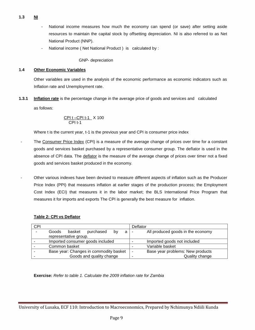
1.3 NI
- National income measures how much the economy can spend (or save) after setting aside
resources to maintain the capital stock by offsetting depreciation. NI is also referred to as Net
National Product (NNP).
- National income ( Net National Product ) is calculated by :
GNP- depreciation 1.4 Other Economic Variables
Other variables are used in the analysis of the economic performance as economic indicators such as
Inflation rate and Unemployment rate.
1.3.1 Inflation rate is the percentage change in the average price of goods and services and calculated
as follows: CPI t –CPI t-1 X 100 CPI t-1
Where t is the current year, t-1 is the previous year and CPI is consumer price index - The Consumer Price Index (CPI) is a measure of the average change of prices over time for a constant
goods and services basket purchased by a representative consumer group. The defIator is used in the
absence of CPI data. The deflator is the measure of the average change of prices over timer not a fixed
goods and services basket produced in the economy.
- Other various indexes have been devised to measure different aspects of inflation such as the Producer
Price Index (PPI) that measures inflation at earlier stages of the production process; the Employment
Cost Index (ECI) that measures it in the labor market; the BLS International Price Program that
measures it for imports and exports The CPI is generally the best measure for inflation.
Table 2: CPI vs Deflator
CPI Deflator
- Goods basket purchased by a representative group.
- All produced goods in the economy
- Imported consumer goods included - Imported goods not included
- Common basket - Variable basket
- Base year: Changes in commodity basket - Goods and quality change
- Base year problems: New products - Quality change
Exercise: Refer to table 1. Calculate the 2009 inflation rate for Zambia
University of Lusaka, ECF 110: Introduction to Macroeconomics, Prepared by Nchimunya Ndiili Kunda Page 10
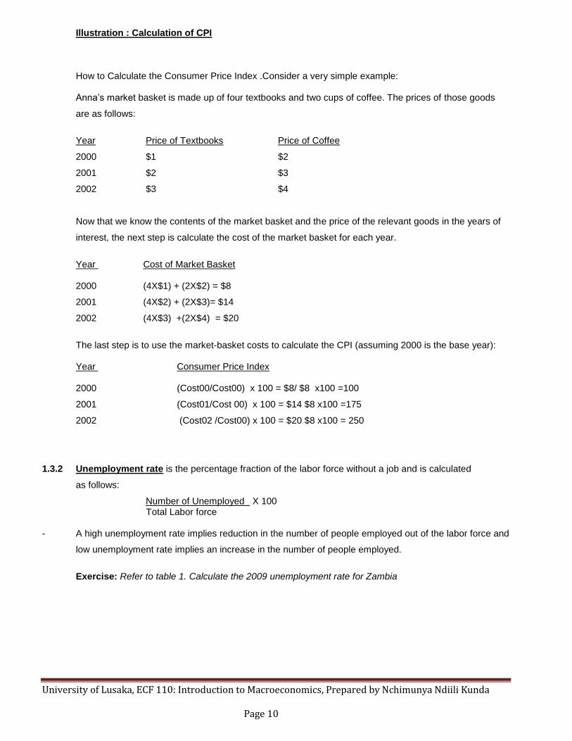
Illustration : Calculation of CPI How to Calculate the Consumer Price Index .Consider a very simple example: Anna‘s market basket is made up of four textbooks and two cups of coffee. The prices of those goods
are as follows:
Year Price of Textbooks Price of Coffee
2000 $1 $2
2001 $2 $3
2002 $3 $4
Now that we know the contents of the market basket and the price of the relevant goods in the years of
interest, the next step is calculate the cost of the market basket for each year.
Year Cost of Market Basket 2000 (4X$1) + (2X$2) = $8
2001 (4X$2) + (2X$3)= $14
2002 (4X$3) +(2X$4) = $20
The last step is to use the market-basket costs to calculate the CPI (assuming 2000 is the base year): Year Consumer Price Index 2000 (Cost00/Cost00) x 100 = $8/ $8 x100 =100
2001 (Cost01/Cost 00) x 100 = $14 $8 x100 =175
2002 (Cost02 /Cost00) x 100 = $20 $8 x100 = 250
1.3.2 Unemployment rate is the percentage fraction of the labor force without a job and is calculated
as follows:
Number of Unemployed X 100 Total Labor force - A high unemployment rate implies reduction in the number of people employed out of the labor force and
low unemployment rate implies an increase in the number of people employed.
Exercise: Refer to table 1. Calculate the 2009 unemployment rate for Zambia
University of Lusaka, ECF 110: Introduction to Macroeconomics, Prepared by Nchimunya Ndiili Kunda Page 11
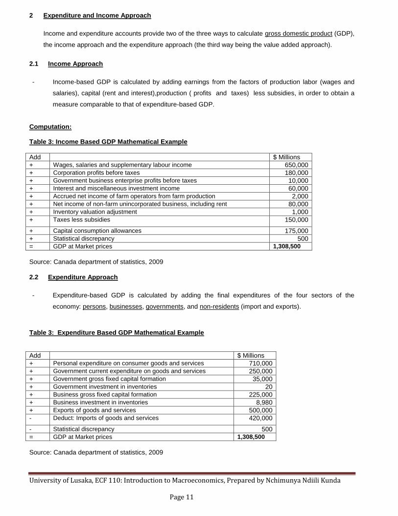
2 Expenditure and Income Approach
Income and expenditure accounts provide two of the three ways to calculate gross domestic product (GDP),
the income approach and the expenditure approach (the third way being the value added approach).
2.1 Income Approach
- Income-based GDP is calculated by adding earnings from the factors of production labor (wages and
salaries), capital (rent and interest),production ( profits and taxes) less subsidies, in order to obtain a
measure comparable to that of expenditure-based GDP.
Computation: Table 3: Income Based GDP Mathematical Example
Add $ Millions
+ Wages, salaries and supplementary labour income 650,000
+ Corporation profits before taxes 180,000
+ Government business enterprise profits before taxes 10,000
+ Interest and miscellaneous investment income 60,000
+ Accrued net income of farm operators from farm production 2,000
+ Net income of non-farm unincorporated business, including rent 80,000
+ Inventory valuation adjustment 1,000
+ Taxes less subsidies 150,000
+ Capital consumption allowances 175,000
+ Statistical discrepancy 500
= GDP at Market prices 1,308,500
Source: Canada department of statistics, 2009
2.2 Expenditure Approach
- Expenditure-based GDP is calculated by adding the final expenditures of the four sectors of the
economy: persons, businesses, governments, and non-residents (import and exports).
Table 3: Expenditure Based GDP Mathematical Example
Add $ Millions
+ Personal expenditure on consumer goods and services 710,000
+ Government current expenditure on goods and services 250,000
+ Government gross fixed capital formation 35,000
+ Government investment in inventories 20
+ Business gross fixed capital formation 225,000
+ Business investment in inventories 8,980
+ Exports of goods and services 500,000
- Deduct: Imports of goods and services 420,000
- Statistical discrepancy 500
= GDP at Market prices 1,308,500
Source: Canada department of statistics, 2009

University of Lusaka, ECF 110: Introduction to Macroeconomics, Prepared by Nchimunya Ndiili Kunda Page 12
2.3 National Income Account Computation
- The national Income account is constructed from business accounts .In the business income statement
the left hand side shows the sales of Goods ( output) and right hand side shows the cost of production and
( wages rents which are earnings).The National account then adds up the aggregates of number of
identical firms to obtain total GDP ( See page 427 ,Samuelson ,2007).
- Note that the GPD the Expenditure (product) side is equal to the GDP from the Income (earnings) side.
Refer to table 3 and 4.
3 Problem in Measuring National Income Using GDP
The famous French economist Alfred Sauvy, points to the fact that GDP excludes (or significantly
underestimates) goods and services produced outside the official market economy. GDP deficiencies can
be divided into four categories:
- Non-market production (household activities) - domestic work and business such tailoring, home based
salons and barbers shops are not accounted for in GDP .There is no way to measure the value added by
these service
- Government services (valuation problems)- In public accounting rules, GDP is the sum of values added by
all economic entities, Thus, value added is in fact constituted by two main parts: wages and profits. In
Government ministries, no value of production is available as public services are generally not bought by
anyone on a market (think of public gardens maintenance or tax collection). A free service resulting from a
past public investment does not appear in GDP
- Informal sector (underground economy) - According to various studies carried out in Zambia, domestic
production could represent as much as 60% of the national outputs
- Voluntary work: a bicycle repaired by a friend makes GDP fall if the work used to be done by (and paid to)
a professional. Thus, a society where voluntary work is widespread will enjoy a higher level of economic
well-being but not necessarily a higher GDP (in fact, even a lower GDP
- Other deficiencies
o GDP and economic well-being – GDP only considers the positive side of production and
not the negative externalities of production. These contribute to environmental
degradation, pollution, poor heath and subsequently an increase economic cost.
o GDP and non-economic well-being (welfare) – There are numerous technical difficulties
in the measurement of distribution of income and wealth, life expectancy and health,
education and access to education that possess varies in Human Development Index
(HDI) for developing and developed countries.
University of Lusaka, ECF 110: Introduction to Macroeconomics, Prepared by Nchimunya Ndiili Kunda Page 13
UNIT: 3
TOPIC: NATIONAL INCOME
LEARNING OBJECTIVE:
At the end of the lesson, students must understand the components of demand at national level and apply the
expenditure and multiplier model to explain national Income equilibrium. Finally they should understand the
relationship between savings and investments decisions.
SUB- TOPICS:
- Aggregate demand and output
- Aggregate Expenditure model
- National Income equilibrium
- The multiplier model
- Paradox of shits -Savings & Investments
1 Aggregate demand and output
1.1 Definition and determinants of AD
1.1.1 Definitions
- Aggregate demand (AD) is the total demand for final goods and services in the economy (Y) at a given
time and price level. It is the amount of goods and services in the economy that will be purchased at all
possible price levels – Keynes
- The total amount that different sectors in the economy are willingly spend in a given period and it
depends on levels of prices - Samuelson
1.1.2 Determinants of AD
- We assume that what is produced (Y) is equal to what is demanded (AD)
- In a closed economy without a government and foreign sector, sources of AD are Consumption (C) and
Investments (I)
AD =C + I
- In a closed economy with a government, sources of AD are Consumption (C) Investments (I) and
government spending ( G)
AD = C+I + G
- Open economy – according to Mundell- Fleming, there are four major components of aggregate demand. The
equation for aggregate demand is Y = C(Y - T) + I(r) + G + NX(e), where
Y represents income or output.
C(Y - T) represents consumption as a function of disposable income, defined as income
Less tax
I(r) represent investment as a function of the interest rate,
G represents government spending,
NX (e) represents net exports, defined as exports less imports (X-IM)

University of Lusaka, ECF 110: Introduction to Macroeconomics, Prepared by Nchimunya Ndiili Kunda Page 14
1.1.3 Downward sloping AD Curves
- The aggregate demand curve is a just like any other demand curve, but for the sum total of all goods and
services in an economy. The aggregate demand curve can be thought of just like a demand curve for a firm.
When the price level is high, aggregate demand is low; when the price level is low, aggregate demand is high
- It shows a downward slope with price level on the vertical axis and income or output on the horizontal axis.It
curve lies in a plane consisting of the price level and income or output.
- The aggregate demand curve outlines the relationship between income or output and the price level. It is
important to notice that aggregate demand is a schedule because as the price level changes, the
income or output also changes
Figure 1: AD Curve
P
250
200
150
100 AD
50
Q
2000 3000 4000 5000
Real GDP (billions)
Source: Samuelson, 2007
- The AD curve represents the quantity of total spending at different price levels, with other factors held
constant.
- The aggregate demand curve is downward sloping. There are a number of reasons for this relationship.
A downward sloping aggregate demand curve means that as the price level drops, the quantity of output
demanded increases. Similarly, as the price level drops, the national income increases
- The equation for aggregate demand of Y = C(Y - T) + I(r) + G + NX(e) has been deciphered. This
equation has many meanings such as output, national income, and GDP.
Exercise: Why is the AD downward sloping?
P
r
i
c
e
f
o
r
c
o
m
m
o
d
i
t
i
e
s

University of Lusaka, ECF 110: Introduction to Macroeconomics, Prepared by Nchimunya Ndiili Kunda Page 15
1.1.4 Shifts in the AD Curves
A change in factors affecting any one or more components of aggregate demand, households (C), firms (I), the
government (G) or overseas consumers and business (X) changes planned aggregate demand and results in a
shift in the AD curve
Figure 2: Shifts in the AD Curve
Source: Geoff Riley, 2006
- The diagram above which shows an inward shift of AD from AD1 to AD3 and an outward shift of AD from AD1 to
AD2. The increase in AD might have been caused by a fall in determinant of AD or an increase in the determinant of
AD.

University of Lusaka, ECF 110: Introduction to Macroeconomics, Prepared by Nchimunya Ndiili Kunda Page 16
Table 4: Summary of the causes in the AD Curve shits
Factors causing a shift in AD
Changes in Expectations
Current spending is affected by
anticipated future income, profit, and
inflation
- The expectations of consumers and businesses can have a powerful effect
on planned spending in the economy E.g. expected increases in consumer
incomes, wealth or company profits encourage households and firms to
spend more – boosting AD. Similarly, higher expected inflation encourages
spending now before price increases come into effect - a short term boost to
AD.
- When confidence turns lower, we expect to see an increase in saving and
some companies deciding to postpone capital investment projects because of
worries over a lack of demand and a fall in the expected rate of profit on
investments.
Changes in Monetary Policy – i.e. a
change in interest rates
(Note there is more than one interest rate
in the economy, although borrowing and
savings rates tend to move in the same
direction)
- An expansionary monetary policy will cause an outward shift of the AD curve.
If interest rates fall – this lowers the cost of borrowing and the incentive to
save, thereby encouraging consumption. Lower interest rates encourage
firms to borrow and invest.
- There are time lags between changes in interest rates and the changes on
the components of aggregate demand.
Changes in Fiscal Policy
Fiscal Policy refers to changes in
government spending, welfare benefits
and taxation, and the amount that the
government borrows
- For example, the Government may increase its expenditure e.g. financed by
a higher budget deficit, - this directly increases AD
- Income tax affects disposable income e.g. lower rates of income tax raise
disposable income and should boost consumption.
- An increase in transfer payments rises AD – particularly if welfare recipients
spend a high % of the benefits they receive
Economic events in the international
economy
International factors such as the exchange
rate and foreign income (e.g. the
economic cycle in other countries)
- A fall in the value of the kwacha (a depreciation) makes imports dearer and
exports cheaper thereby discouraging imports and encouraging exports – the
net result should be that ZMK AD rises – the impact depends on the price
elasticity of demand for imports and exports and also the elasticity of supply
of ZMK exporters in response to an exchange rate depreciation.
- An increase in overseas incomes raises demand for exports and therefore
ZMK AD rises. In contrast a recession in a major export market will lead to a
fall in ZMK exports and an inward shift of aggregate demand.The ZMK is an
open economy, meaning that a large and rising share of our national output is
linked to exports of goods and services or is open to competition from
imports.
Changes in household wealth
Wealth refers to the value of assets
owned by consumers e.g. houses and
shares
- A rise in house prices or the value of shares increases consumers‘ wealth
and allow an increase in borrowing to finance consumption increasing AD. In
contrast, a fall in the value of share prices will lead to a decline in household
financial wealth and a fall in consumer demand.

University of Lusaka, ECF 110: Introduction to Macroeconomics, Prepared by Nchimunya Ndiili Kunda Page 17
2 Aggregate Expenditure Model
2.2.1 Definition - Aggregate expenditure (AE) is the sum of consumption, investment, government purchases, and net export. Of
these four sectors, the consumption represents the largest share.
2.2.2 The consumption function
- The consumption function shows the positive relationship between disposable income and consumption demand. It
shows aggregate consumption demand at each level of personal disposable income
C = Co + MPC (Yd), where :
C = total consumption
Co = autonomous consumption demand whose amount is independent of disposable income
MPC = marginal propensity to consume is a fraction of each extra pound of disposable income that household wish to
Consume, The remaining (1- 0) they wish to save . This is a fraction between 0 and 1; It is equal to change in
consumption brought about by a change in disposable income. It is the slope of the consumption function.
MPC = change in C / change in Yd ) , where
Yd = disposable income.
Figure 3: Consumption Function
C = consumption function
Consumers‘ Expenditure
Slope = MPC = C / Yd
Co
Disposable income ( Yd)
Source: Begg.D,2007

University of Lusaka, ECF 110: Introduction to Macroeconomics, Prepared by Nchimunya Ndiili Kunda Page 18
- Therefore S+ C = Yd, planned saving is part of income not planned to be spent on consumption
2.2.3 The Saving function
- The saving function shows the desired saving at each income level. Saving is income not consumed The saving
function is derived from the consumption function :
S= -Co + ( 1- MPC) Yd
Figure 4 : Saving Function
S = - Co + ( 1 – MPC)Yd
Saving
0
- A
Income
Source: Begg. D, 2007
- MPS = marginal propensity to save is equal to change in savings (S) brought about by a change in disposable
income.
MPS = change in S / change in Yd
MPS = 1 - MPC
- Since all income must be either consumed or saved, then any change in income must also be consumed or saved.
Therefore: MPC + MPS = 1
- The average propensity to consume (APC) is the portion of income spent on consumption.
(APC = C / Yd)
- The average propensity to save (APS) is the portion of income saved.
(APS = S / Yd)
Again, APC + APS = 1

University of Lusaka, ECF 110: Introduction to Macroeconomics, Prepared by Nchimunya Ndiili Kunda Page 19
3 National Income Equilibrium
3.1 Definition
- Equilibrium is when planned saving equals actual output and actual income – Begg. D
Equilibrium of National Income(Y) is the level of output whose production will create total spending just
sufficient to purchase that output. If the economy produces an amount of goods that differs to the
amount that the four sectors of the economy buy (AE), AE and aggregate production (AP) are not equal;
then the economy is in disequilibrium.
Figure 5: Line diagram and equilibrium Output
AD =C + I C
Desired
Spending E
0 C
- A
45
Y¹ Y*
Source: Begg, 2007
- The 45 line reflects any value on the horizontal axis onto the same value of the vertical axis. Point E,
where AD schedule crosses the 45 line is the point where AD is equal to income. Therefore E is the
equilibrium point at which planned spending equals actual output and actual income.
- All output below E are Y*, aggregate demand exceeds income and output and output above E implies
that AD is less than income and output.
Adjustments towards equilibrium
- When output (Y) is above E output (Y*) this implies that AE < AP, firms will involuntarily accumulate
inventory. This will signal firms that they have overproduced. As a result, firms will cut back on
production and/or prices. This will decrease the total value of output, moving the economy towards the
equilibrium GDP.
- When output (Y¹) is below E output (Y*) this implies that AE > AP, inventories will be depleted
unexpectedly. This will signal firms that they have not produced enough. As a result, firms will increase
productions and/or prices. This will increase the total value of output, moving the economy towards the
equilibrium GDP.
B

University of Lusaka, ECF 110: Introduction to Macroeconomics, Prepared by Nchimunya Ndiili Kunda Page 20
4 The Multiplier Model
- The multiplier model is the ratio of the change in equilibrium output to the change in autonomous
spending that caused the change ( Begg , 2007).It tells how much output has changed after a shift in
AD. Recall that AD =C + I. In this analysis we will focus on a parallel shift in the AD schedule caused by
a change in autonomous investments demand.
- The multiplier depends on the MPC; Keynes observed that changes in autonomous expenditures (those
expenditures independent of income) could create even larger changes in national income. Therefore, a
large change in MPC , the multiplier is small or vice versa.
Multiplier = 1 / (1- MPC) =1/MPS
- For example, a technological breakthrough has increased the autonomous investment by $50million, this
$50M will become the income of the resources market. Workers who may have higher income are willing
to spend more in the market. Their spending becomes the income of producers who will again spend in
the market, and create extra income. This process repeats itself, creating a multiplier effect. If the
Multiplier (M) = 2.5, then the aggregate expenditure will increase by $50M X 2.5 = $ 125M.
4.1 Equilibrium using the Multiplier Models
The equilibrium between AE and AP and the multiplier model is illustrated below.
Table 5: Data in this table is used to construct the graph below.
GDP CONSUMPTION GDP=C+I SAVING INVESTMENT
240 244 264 -4 20
260 260 280 0 20
280 276 296 4 20
300 292 312 8 20
320 308 328 12 20
340 324 344 16 20
360 340 360 20 20
380 356 376 24 20
400 372 392 28 20

University of Lusaka, ECF 110: Introduction to Macroeconomics, Prepared by Nchimunya Ndiili Kunda Page 21
Figure 6: The equilibrium between AE and AP ( AE & Y)
- The investments has increased the equilibrium GDP, (from the intersection of red and blue curves (A) to
the new intersection of red and yellow curves (B).The same equilibrium GDP can be obtained by
observing the Investment and Saving schedule.

University of Lusaka, ECF 110: Introduction to Macroeconomics, Prepared by Nchimunya Ndiili Kunda Page 22
Figure 7: Equilibrium using Investments and saving Model and multiplier Model
- In both graphs, we can see that equilibrium GDP is at 360.
- Another approach to get the equilibrium GDP is by using the multiplier. The equilibrium GDP, GDPe,
before the investment is 260. MPC for this data set is 0.8.
Multiplier = 1 / 1-MPC = 1 / (1-0.8) = 5
The investment amount of 20, will increase GDPe by 5 times, this will give us an increase of
20 X 5 = 100.Therefore, the new equilibrium GDP will be 260 + 100 = 360.
5 The Paradox of thrift
- Paradox of thrift is the change in the amount households wish to save of each income leads to a change
in E income, but no change in equilibrium saving which must be equal planned investments ( Begg,
2007).In this analysis, we will focus on a parallel shift in the AD schedule caused by a change in in the
autonomous consumption and savings.
- A higher autonomous consumption demand implies an identical fall in autonomous planned saving .For
example, if automous consumption increases by 5 , there is a parallel shift in the consumption function
and AD but a parallel downward shift in the saving function fall .
- In Equilibrium: Planned S = Planned I ( investment is not altered).
Therefore at E, income must always adjust to restore planned savings to the unchanged level of planned
investments.
Co CF AD S

University of Lusaka, ECF 110: Introduction to Macroeconomics, Prepared by Nchimunya Ndiili Kunda Page 23
Figure 8: The paradox of thrift (Savings & Investments)
S S¹
Savings E E¹
0
Y* Y**
Source: Begg, D, 2007
- In equilibrium, planned savings equals planned investments. A fall in the desire to save induces a rise in
output to keep planned saving equal to planned investments.
University of Lusaka, ECF 110: Introduction to Macroeconomics, Prepared by Nchimunya Ndiili Kunda Page 24
UNIT: 4
TOPIC: FISCAL POLICY
LEARNING OBJECTIVE:
Students must understand the instruments used by the Government under fiscal policy in stabilizing the
economy.
Students must apply the applicable fiscal policy in an economic situation to stabilize the economy.
SUB- TOPICS:
- Goals of fiscal policy
- Tools of Fiscal policy
o Government spending
o Taxes
- Fiscal Policy Expansion and Contraction
- Effects of Governments spending and taxes on output
- Crowding out effect
- Fiscal Policy and budget deficit:
o Government and Structural budget
o Budget deficits adjustments
- The national debt and the deficit
- Limitations of Fiscal policy
1. GOALS OF FISCAL POLICY
- Fiscal policy is one of the instruments that government uses to stabilize the economy. The policy can be
used to reduce inflation, unemployment, improve economic growth or correct trade balance. Fiscal policy
consists of managing the national Budget and its financing so as to influence economic activity
(Samuelson. N, 2006)
- This entails the expansion or contraction of government expenditures related to specific government
programs. It also includes the raising of taxes to finance government expenditures and the raising of
debt (bonds & treasury bills) to bridge the gap (Budget deficit) between revenues (tax receipt) and
expenditures related to the implementation of government programs.
1.1 Tools of fiscal Policy
- The tools of Fiscal policy are taxes and government spending:
• Government spending entails government expenditures related to specific government
programs
• Taxes is the raising or reduction of taxes to finance government expenditures

University of Lusaka, ECF 110: Introduction to Macroeconomics, Prepared by Nchimunya Ndiili Kunda Page 25
- Government spending affects the overall spending in the economy, while taxes affect individuals
disposable income and prices of goods and factors of production.
2. Fiscal Policy Expansion and Contraction
2.1 Fiscal Policy Expansion
- Fiscal policy expansion is when government spending is increased to increase output. Taxes are
reduced to increase disposable income to increase aggregate demand (AD) and output. Fiscal policy
expansion is adopted during recession to foster economic growth.
- Lowering taxes and increasing the Budget Deficit is considered an expansive fiscal policy that would
increase aggregate demand and stimulate the economy.
Figure 1: Fiscal policy expansion
P² B
P¹ A
AD 1 AD2
Y ¹ Y²
Source: Blanchard. O, 2007
When government spending is increased or taxes are reduced AD increases from AD1 to AD 2, output
increases from Y¹ to Y² and general prices increase from P¹ to P². Therefore overall economic activity
increases when fiscal policy expansion is implemented.

University of Lusaka, ECF 110: Introduction to Macroeconomics, Prepared by Nchimunya Ndiili Kunda Page 26
2.2 Fiscal Policy Contraction
Fiscal policy contract is when government spending is reduced to decrease output. Taxes are increased
to reduce disposable income and aggregate demand (AD) .Subsequently output is reduced. Fiscal policy
contraction is adopted during a boom to slow down economic growth.
- Raising taxes and reducing the Budget Deficit is deemed to be a restrictive fiscal policy as it would
reduce aggregate demand and slow down GDP growth.
Figure 2: Fiscal policy contraction
P¹
B
A
P²
AD 2 AD1
Y² Y ¹
Source: Blanchard. O, 2007
When government spending is reduced or taxes are increased AD reduces from AD1 to AD 2, output
reduces from Y¹ to Y² and general prices reduce from P¹ to P². Therefore overall economic activity
slows down when fiscal policy contraction is implemented.
3. EFFECTS OF GOVERNMENT SPENDING AND TAXES ON OUTPUT
3.1 Under fiscal policy expansion
- Increase in government spending leads to an increase in output. This eventually leads to an increase in
employment .Therefore AD and prices also rise.

University of Lusaka, ECF 110: Introduction to Macroeconomics, Prepared by Nchimunya Ndiili Kunda Page 27
- Reduction in taxes leads to an increase in the disposable income of individuals. This increases the AD
and stimulates economic activities (output increases).
3.2 Under Fiscal Contraction
- Reduction in government spending leads to a decrease in output. This eventually leads to decrease in
employment ,AD and prices also fall down.
- Increase in taxes leads to a reduction in the disposable income of individuals. This decreases the AD
and slows down economic activities (output reduces).
4. CROWDING OUT EFFECT
- As government spend more to correct the recessionary gap in the economy, they compete with private
sector for resources and goods and services.
- As government expenditure increases, consumption and investment decreases, causing the
ineffectiveness of the fiscal policy.
- Another way of defining crowding out effect is when government increases spending and reduces
taxation, resulting in a deficit which must be funded through borrowing. This increased borrowing will
push the interest rate higher, reducing the consumption and investment in the private sector.
Figure 3: Crowding out effect
P² B
P¹ A C
AD 1 AD2
Y ¹ Y³ Y²
Source: Blanchard. O, 2007
University of Lusaka, ECF 110: Introduction to Macroeconomics, Prepared by Nchimunya Ndiili Kunda Page 28
- At the same level of prices, an increase in government spending will lead to an immediate shift of AD
from point A to Point C at AD2.Output will automatically increase from Y¹ to Y².A t point C, government
will start competing with private sector for resources and goods and services. Therefore part of the
investment sector will fall out of business and output will reduce from Y² to Y³. This will also lead to a fall
in AD 2 along the same demand curve from point C to B. The fall of output from Y² to Y³ and aggregate
demand from point C to B is referred to as crowding out effect.
5. FISCAL POLICY AND BUDGET DEFICIT
- Budget deficit is a shortfall between Government revenue – expenditure. This is when government
expenditure is less that the revenue. The source of government revenue is taxes.
- Therefore raising of taxes to finance government expenditure is a good measure to reduce budget deficit
(Fiscal contraction).
- Lowering taxes and increasing government spending is considered an expansive fiscal policy that would
increase aggregate demand and stimulate the economy. However, this leads to an increase in the
Budget Deficit.
5.1 Budget deficits adjustments
- The budget deficit should be adjusted to the structural budget level .The structural budget shows a
balanced budget where the government expenditure is equal to revenue (what the budget would be like
if output were at potential output.)
- Given that higher government spending on goods and services increases equilibrium. Given a tax rate,
revenue rises but the deficit increases. (Note that budget deficit may not be necessarily be connected to
fiscal stance. A deficit may occur during a recession due to low output and the deficit is larger than in the
boom.) .
- Budget deficit corrective measure is to impose a higher tax rate that will reduce disposable income and
affect costs of factors of production. This will lead to a reduction in AD and output taking the equilibrium
output to the equilibrium output point (structural budget).Therefore the budget deficit is reduced.
- Alternatively government spending can be reduced which is a very rare measure taken to correct budget
deficit.
University of Lusaka, ECF 110: Introduction to Macroeconomics, Prepared by Nchimunya Ndiili Kunda Page 29
6. THE NATIONAL DEBT AND THE BUDGET DEFICT
- When government implements an expansionary fiscal policy, Government increases spending and
reduces taxation. This results in a budget deficit which must be funded through borrowing since taxes
are reduced.
- Therefore government resorts to borrowing and national debt is created.
7. LIMITATIONS OF FISCAL POLICY
- Lowering taxes and increasing government spending is considered an expansive fiscal policy that would
increase aggregate demand and stimulate the economy. This is a restrictive fiscal policy as it would
reduce aggregate demand and slow down GDP growth despite increasing government revenue. This is
referred to as crowding out effect.
- Lowering taxes and increasing government spending is considered an expansive fiscal policy that would
increase aggregate demand and stimulate the economy. However, this leads to an increase in the
Budget Deficit.
- Budget deficit which must be funded through borrowing since taxes are reduced leads to an increase in
national debt.
University of Lusaka, ECF 110: Introduction to Macroeconomics, Prepared by Nchimunya Ndiili Kunda Page 30
UNIT: 5
TOPIC: MONETARY POLICY
LEARNING OBJECTIVE:
Students must understand the instruments used by the Government under monetary policy in stabilizing
the economy.
Students must apply the applicable monetary policy in an economic situation to stabilise the economy.
SUB- TOPICS:
- Goals of monetary policy
- Tools of monetary policy
o Discount rate
o Reserve ratio
o Open markets operations
- Monetary policy expansion and contraction ( IS –LM Model)
- Monetary policy in the open market
1. GOALS OF MONETARY POLICY
- Monetary policy is one of the instruments that government uses to stabilize the economy. The policy can
be used to manage or curb domestic inflation and control money supply. Monetary policy consists of
managing discount rates, reserve requirement for commercial banks and open market operations in the
economy (Samuelson. N, 2006).
- Monetary policy is implemented by the central bank of every country (Bank of Zambia in Zambia).
Recently, the Central banks have often focused on a second objective, that is managing economic
growth as both inflation and economic growth are highly interrelated.
2. Tools of Monetary Policy
- The tools of monetary policy are discount rates, statutory reserve ratios and open market operations.
o Discount rate is interest rate overnight cash rate for lending money to commercial banks
by the central bank. The central bank controls the monetary base by either reducing or
increasing the discount rate when lending money to banks.
o Statutory reserve ratio is the statutory minimum amount every commercial bank is
required to have at the central bank. The central bank controls the monetary base by
either reducing or increasing the required reserve ratio.
University of Lusaka, ECF 110: Introduction to Macroeconomics, Prepared by Nchimunya Ndiili Kunda Page 31
o The open market operations is the selling of treasury bill and bonds to the market with
interest to the public. Treasury bills are short term with a maturity period of within one
year. Bonds are long term with maturity period after one year. The central bank controls
the money in circulation by either selling or buying bonds and treasury bills.
3. Monetary Policy Expansion and Contraction
3.1 Monetary Policy Expansion
- Monetary policy expansion is when
o Discount rate is reduced to increase money supply in circulation. The cost of borrowing
for commercial banks from the central bank is reduced leading to an increase in the
money borrowed. The reduced discount rates trickle down to low interest rates charged
by the commercial banks to the public. This leads to an increment in borrowing from
the commercial and Investment in the economy increases.
o Reserve ratios are reduced to increase money supply in circulation .The commercial
banks monetary base will increase .Therefore money to given to the public will increase.
o Bonds and treasury bills are bought from the public in exchange for money .This leads
to an increase in money in circulation and fosters economic growth.
- Monetary policy expansion is adopted during recession to foster economic growth.
University of Lusaka, ECF 110: Introduction to Macroeconomics, Prepared by Nchimunya Ndiili Kunda Page 32
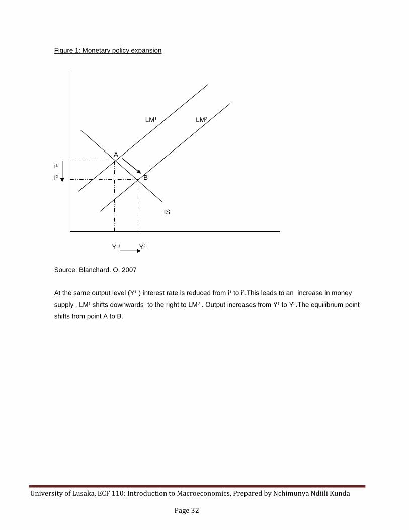
Figure 1: Monetary policy expansion
LM¹ LM²
A
i¹
i² B
IS
Y ¹ Y²
Source: Blanchard. O, 2007
At the same output level (Y¹ ) interest rate is reduced from i¹ to i².This leads to an increase in money
supply , LM¹ shifts downwards to the right to LM² . Output increases from Y¹ to Y².The equilibrium point
shifts from point A to B.
University of Lusaka, ECF 110: Introduction to Macroeconomics, Prepared by Nchimunya Ndiili Kunda Page 33
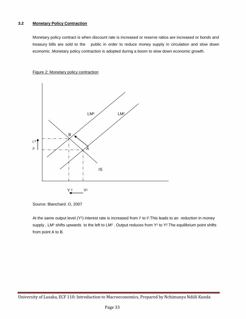
3.2 Monetary Policy Contraction
Monetary policy contract is when discount rate is increased or reserve ratios are increased or bonds and
treasury bills are sold to the public in order to reduce money supply in circulation and slow down
economic .Monetary policy contraction is adopted during a boom to slow down economic growth.
Figure 2: Monetary policy contraction
LM² LM¹
B
i ²
i¹ A
IS
Y ² Y¹
Source: Blanchard. O, 2007
At the same output level (Y¹) interest rate is increased from i¹ to i².This leads to an reduction in money
supply , LM¹ shifts upwards to the left to LM² . Output reduces from Y¹ to Y².The equilibrium point shifts
from point A to B.
University of Lusaka, ECF 110: Introduction to Macroeconomics, Prepared by Nchimunya Ndiili Kunda Page 34
UNIT: 6
TOPIC: MONEY AND BANKING
LEARNING OBJECTIVE:
Students must know the types of money and how money is created in the economy. The functions of the
central bank and the commercial banks will also be analyzed in detail.
At the end of the lesson, students must be conversant of the demand for money arises and how money
is supplied to meet the demand.
SUB- TOPICS:
- Definition and functions of money
- Types of money
- The demand for money
- The supply for money
o The central bank
o The functions of the commercial banks
- Creation of money
o Multiple deposit expansion
o Money multiplier
1. DEFINITION AND FUNCTIONS OF MONEY
1.1 Definition of Money
- Money is any good that is widely used and accepted in transactions involving the transfer of goods
and services from one person to another. Economists differentiate among three different types of
money: commodity money, fiat money, and bank money.
- Commodity money is a good whose value serves as the value of money. Gold coins are an
example of commodity money. In most countries, commodity money has been replaced with fiat
money.
- Fiat money is a good, the value of which is less than the value it represents as money. Dollar bills
are an example of fiat money because their value as slips of printed paper is less than their value
as money.
University of Lusaka, ECF 110: Introduction to Macroeconomics, Prepared by Nchimunya Ndiili Kunda Page 35
- Bank money consists of the book credit that banks extend to their depositors. Transactions made
using checks drawn on deposits held at banks involve the use of bank money.
1.2 FUNCTIONS OF MONEY
Money is used as a medium of exchange, store of value and unit of account
1.2.1 Medium of exchange
- Money's most important function is as a medium of exchange to facilitate transactions. Without
money, all transactions would have to be conducted by barter, which involves direct exchange of
one good or service for another. The difficulty with a barter system is that in order to obtain a
particular good or service from a supplier, one has to possess a good or service of equal value,
which the supplier also desires.
- In other words, in a barter system, exchange can take place only if there is a double coincidence
of wants between two transacting parties. The likelihood of a double coincidence of wants,
however, is small and makes the exchange of goods and services rather difficult. Money effectively
eliminates the double coincidence of wants problem by serving as a medium of exchange that is
accepted in all transactions, by all parties, regardless of whether they desire each others' goods
and services.
1.2.2 Store of value
- In order to be a medium of exchange, money must hold its value over time; that is, it must be a
store of value. If money could not be stored for some period of time and still remain valuable in
exchange, it would not solve the double coincidence of wants problem and therefore would not be
adopted as a medium of exchange. As a store of value, money is not unique; many other stores of
value exist, such as land, works of art, and even baseball cards and stamps. Money may not even
be the best store of value because it depreciates with inflation.
- However, money is more liquid than most other stores of value because as a medium of
exchange, it is readily accepted everywhere. Furthermore, money is an easily transported store of
value that is available in a number of convenient denominations.

University of Lusaka, ECF 110: Introduction to Macroeconomics, Prepared by Nchimunya Ndiili Kunda Page 36
1.2.3 Unit of account
- Money also functions as a unit of account, providing a common measure of the value of goods and
services being exchanged. Knowing the value or price of a good, in terms of money, enables both
the supplier and the purchaser of the good to make decisions about how much of the good to
supply and how much of the good to purchase.
2. DEMAND FOR MONEY
The demand for money is affected by several factors, including the level of income, interest rates,
and inflation as well as uncertainty about the future. The way in which these factors affect money
demand is usually explained in terms of the three motives for demanding money: the transactions,
the precautionary, and the speculative motives.
2.1 Transactions motive
The transactions motive for demanding money arises from the fact that most transactions involve
an exchange of money. Because it is necessary to have money available for transactions, money
will be demanded. The total number of transactions made in an economy tends to increase over
time as income rises. Hence, as income or GDP rises, the transactions demand for money also
rises.
2.1 Precautionary motive
People often demand money as a precaution against an uncertain future. Unexpected expenses,
such as medical or car repair bills, often require immediate payment. The need to have money
available in such situations is referred to as the precautionary motive for demanding money.
2.3 Speculative motive
- Money, like other stores of value, is an asset. The demand for an asset depends on both its rate of
return and its opportunity cost. Typically, money holdings provide no rate of return and often
depreciate in value due to inflation. The opportunity cost of holding money is the interest rate that
can be earned by lending or investing one's money holdings. The speculative motive for
demanding money arises in situations where holding money is perceived to be less risky than the
alternative of lending the money or investing it in some other asset.
- For example, if a stock market crash seemed imminent, the speculative motive for demanding
money would come into play; those expecting the market to crash would sell their stocks and hold
University of Lusaka, ECF 110: Introduction to Macroeconomics, Prepared by Nchimunya Ndiili Kunda Page 37
he proceeds as money. The presence of a speculative motive for demanding money is also
affected by expectations of future interest rates and inflation. If interest rates are expected to rise,
the opportunity cost of holding money will become greater, which in turn diminishes the speculative
motive for demanding money. Similarly, expectations of higher inflation presage a greater
depreciation in the purchasing power of money and therefore lessen the speculative motive for
demanding money.
3. SUPPLY OF MONEY
- There are several definitions of the supply of money. M1 is narrowest and most commonly used.
It includes all currency (notes and coins) in circulation, all checkable deposits held at banks
(bank money), and all traveler's checks. A somewhat broader measure of the supply of money is
M2, which includes all of M1 plus savings and time deposits held at banks. An even broader
measure of the money supply is M3, which includes all of M2 plus large denomination, long-term
time deposits—for example, certificates of deposit (CDs) in amounts over $100,000. Most
discussions of the money supply, however, are in terms of the M1 definition of the money supply.
3.1 The Central Bank and the supply of money
- A portion of each nation's money supply ( M1) is controlled by a government agency known as the
central bank. The central bank is unique in that it is the only bank that can issue currency. The Zambian
central bank is called the Bank of Zambia (BOZ) .The Bank of Zambia issues all Zambian Kwacha bills,
known as Federal Reserve Notes. Thus, BOZ has control over the supply of the national currency. BOZ
also has control over the private bank reserves that banks entrust to the central bank. Banks hold a
portion of their required reserves with the central bank because BOZ acts as a clearing house for all
sorts of transactions between banks—for example, the processing of all checks.
-
- The central bank's liabilities therefore consist of all kwacha notes in circulation plus all private bank
deposits held at the central bank as reserves On the asset side, BOZ owns a large amount of
government debt in the form of government bonds. These bonds have been issued by the Treasury to
pay for current and past government deficits. A simplified example of the central bank's balance sheet is
provided in Table 1. Note that the central bank's total liabilities are equal to its total assets.
TABLE 1: The Balance Sheet of A central Bank ($ values are in millions)
Assets Liabilities
Government bonds $300 Central bank Reserve notes $250
Reserves of private 50
banks
- The central bank's control over the money supply stems from its ability to change the composition of its
balance sheet. For example, the central bank may decide to purchase additional government bonds on

University of Lusaka, ECF 110: Introduction to Macroeconomics, Prepared by Nchimunya Ndiili Kunda Page 38
the open market from bondholders or private banks. This type of action is referred to as an open market
operation by the central bank. In exchange for these government bonds, the central bank increases the
reserves of private banks by the amount of the purchase.
-
- Banks, in turn, lend out their excess reserves and initiate the multiple deposit expansion process
discussed above. Thus, when the central bank buys government bonds on the open market, it increases
the supply of money by increasing bank reserves and inducing an expansion in the amount of deposits.
Similarly, when the central bank sells some of its stock of government bonds to bondholders or private
banks, the central bank compensates itself for the sale by reducing the reserves of private banks. The
sale of government bonds by the central bank reduces the supply of money by reducing the reserves
available to private banks and thereby decreasing the amount of deposit expansion that is possible.
- The central bank can also control the supply of money by its choice of the reserve requirement. Recall
that the money multiplier is the reciprocal of the reserve requirement. If the central bank increases the
reserve requirement, the money multiplier decreases, implying that deposit creation and the money
supply are reduced. If the central bank decreases the reserve requirement, the money multiplier
increases, causing both the creation of deposits and the money supply to expand further.
3.2 The commercial banks
- In order to understand the factors that determine the supply of money, one must first understand the role
of the banking sector in the money-creation process. Banks perform two crucial functions. First, they
receive funds from depositors and, in return, provide these depositors with a checkable source of funds
or with interest payments. Second, they use the funds that they receive from depositors to make loans to
borrowers; that is, they serve as intermediaries in the borrowing and lending process.
-
- When banks receive deposits, they do not keep all of these deposits on hand because they know that
depositors will not demand all of these deposits at once. Instead, banks keep only a fraction of the
deposits that they receive. The deposits that banks keep on hand are known as the banks' reserves.
When depositors withdraw deposits, they are paid out of the banks' reserves. The reserve requirement
is the fraction of deposits set aside for withdrawal purposes. The reserve requirement is determined by
the nation's banking authority, a government agency known as the central bank. Deposits that banks
are not required to set aside as reserves can be lent to borrowers, in the form of loans. Banks earn
profits by borrowing funds from depositors at zero or low rates of interest and using these funds to
make loans at higher rates of interest.
-
- A balance sheet for a typical bank is given in Table 2. The balance sheet summarizes the bank's
assets and liabilities. Assets are valuable items that the bank owns and consist primarily of the bank's
reserves and loans. Liabilities are valuable items that the bank owes to others and consist primarily of
the bank's deposit liabilities to its depositors. In Table 2, the bank's assets (reserves and loans) total $1
University of Lusaka, ECF 110: Introduction to Macroeconomics, Prepared by Nchimunya Ndiili Kunda Page 39
million. The bank's liabilities (deposits) total $1 million. A banking firm's assets must always equal its
liabilities.
TABLE 2: The Balance Sheet of A Typical Bank
Assets Liabilities
Reserves $100,000 Deposits $1,000,000
Loans 900,000
You can infer from Table 2 that the reserve requirement in this example is 10%.
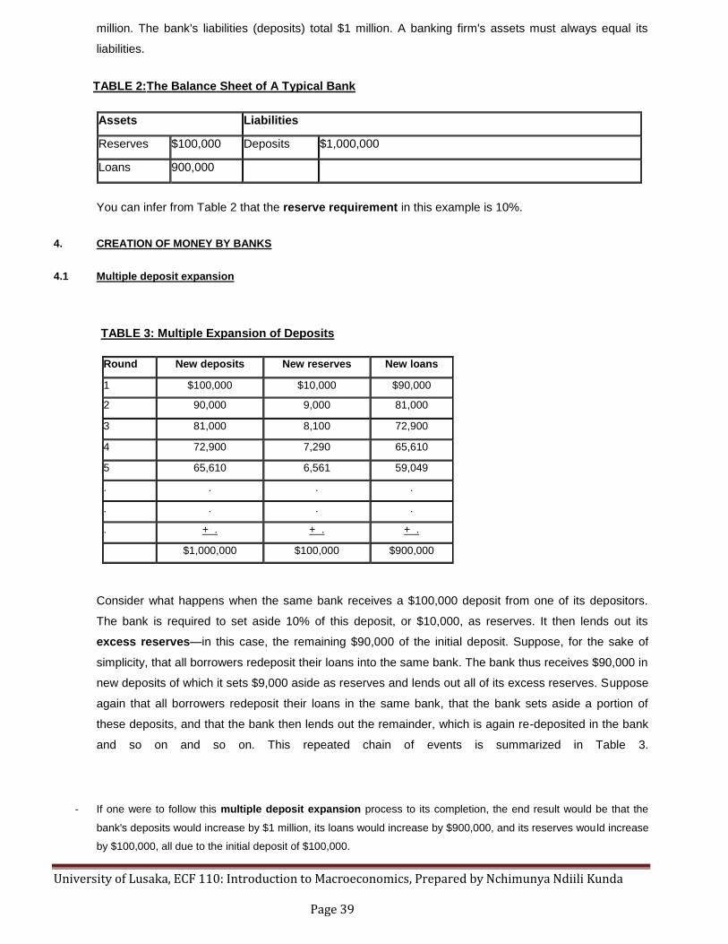
4. CREATION OF MONEY BY BANKS
4.1 Multiple deposit expansion
Consider what happens when the same bank receives a $100,000 deposit from one of its depositors.
The bank is required to set aside 10% of this deposit, or $10,000, as reserves. It then lends out its
excess reserves—in this case, the remaining $90,000 of the initial deposit. Suppose, for the sake of
simplicity, that all borrowers redeposit their loans into the same bank. The bank thus receives $90,000 in
new deposits of which it sets $9,000 aside as reserves and lends out all of its excess reserves. Suppose
again that all borrowers redeposit their loans in the same bank, that the bank sets aside a portion of
these deposits, and that the bank then lends out the remainder, which is again re-deposited in the bank
and so on and so on. This repeated chain of events is summarized in Table 3.
- If one were to follow this multiple deposit expansion process to its completion, the end result would be that the
bank's deposits would increase by $1 million, its loans would increase by $900,000, and its reserves would increase
by $100,000, all due to the initial deposit of $100,000.
TABLE 3: Multiple Expansion of Deposits
Round New deposits New reserves New loans
1 $100,000 $10,000 $90,000
2 90,000 9,000 81,000
3 81,000 8,100 72,900
4 72,900 7,290 65,610
5 65,610 6,561 59,049
. . . .
. . . .
. + . + . + .
$1,000,000 $100,000 $900,000

University of Lusaka, ECF 110: Introduction to Macroeconomics, Prepared by Nchimunya Ndiili Kunda Page 40
4.2 Money Multiplier Effect
The amount by which bank deposits expand in response to an increase in excess reserves is found
through the use of the money multiplier, which is given by the formula
-
In the example of deposit expansion found in Table 3 , the reserve requirement is 10%; so, the money
multiplier in this case is (1/.10) = 10. The excess reserves resulting from the initial deposit of $100,000
are $90,000. Multiplying $90,000 by the money multiplier, 10, yields $900,000, which is the amount of
additional deposits created by the banking system as the result of the initial $100,000 deposit.
- In reality, loan recipients do not deposit all of their loan funds into a bank. More typically, they hold a
fraction of their loan funds as currency. If some loan funds are held as currency, then there is a leakage
of money out of the banking system. In this case, the money multiplier will still be greater than 1, but it
will be less than the inverse of the reserve requirement.
University of Lusaka, ECF 110: Introduction to Macroeconomics, Prepared by Nchimunya Ndiili Kunda Page 41
UNIT: 7
TOPIC: INFLATION
LEARNING OBJECTIVE:
At the end of the lesson, students must be conversant of the costs and benefits of inflation. The focus
will be on the causes, consequences and cures of inflation. Students must know the policies to
implement in order to control inflation and achieve the target inflation.
SUB- TOPICS:
- Definitions of inflation
- Measurement of inflation
- Causes of inflation
- Costs of inflation
- Cures of inflation
1. Definitions of inflation
This is a rise in the general level of prices in a given period of time (Samuelson. N,2006). Other
economists have defined inflation as the persistent rise in relative prices over a given period of time.
Inflation is a normal economic development as long as the annual percentage remains low; once the
percentage rises over a pre-determined level, it is considered an inflation crisis.
- The rate of inflation is the percentage change of general prices in a given period of time.
(Samuelson. N, 2006) and is calculated as follows:
Price level (t) – Price level (t-1) x 100
Price level (t -1 )
Or CPI (t) – CPI (t-1) x 100
CPI (t -1)
Where t = current year
t-1 = previous year
- The government calculates the price level by constructing price indexes such as consumer price index, ,
GDP price index and producer price index

University of Lusaka, ECF 110: Introduction to Macroeconomics, Prepared by Nchimunya Ndiili Kunda Page 42
2. MEASUREMENT OF INFLATION
2.1 Consumer Price Index
- The consumer price index is the most widely used to measure inflation. The Consumer Price Index (CPI)
is a measure of the average change of prices over time for a constant goods and services basket
purchased by a representative consumer group.
The traditional method of constructing a CPI is prices for a market basket goods ( common basket)
such as food, clothing , shelter, transportation purchased for daily use. The index is then constructed by
weighting each price according to the economic performance of the commodity.
- Simple method of calculating CPI
Assume that the market basket has two commodities: textbooks and coffee consumed in quantities of 4
and 2 respectively. The prices of these goods are as follows:
Year Price of Textbooks Price of Coffee
2000 $1 $2
2001 $2 $3
2002 $3 $4
Now that we know the contents of the market basket and the price of the relevant goods in the years of
interest, the next step is calculate the cost of the market basket for each year.
Year Cost of Market Basket 2000 (4X$1) + (2X$2) = $8
2001 (4X$2) + (2X$3)= $14
2002 (4X$3) +(2X$4) = $20
The last step is to use the market-basket costs to calculate the CPI (assuming 2000 is the base year): General formula : Total cost for current year divided by total cost for base year multiply by a hundred. Year Consumer Price Index 2000 (Cost00/Cost00) x 100 = $8/ $8 x100 =100
2001 (Cost01/Cost 00) x 100 = $14 $8 x100 =175
2002 (Cost02 /Cost00) x 100 = $20 $8 x100 = 250
The rate of inflation for 2001 is calculated as follows:
175 -100 x 100 = 75%
100
Note that the CPI for the base year is always 100
University of Lusaka, ECF 110: Introduction to Macroeconomics, Prepared by Nchimunya Ndiili Kunda Page 43
2.2 The GDP deflator
- The defIator is used in the absence of CPI data. The deflator is the measure of the average change of
prices over time not a fixed goods and services basket produced in the economy.
2.3 Producer price index
- Other various indexes have been devised to measure different aspects of inflation such as the Producer
Price Index (PPI) that measures inflation at earlier stages of the production process; The CPI is
generally the best measure for inflation.
3. CAUSES OF INFLATION
There are many causes for inflation and these depend on a number of factors.
3.1 Quantity Theory of Money
The quantity theory of money states that there is a direct relationship between the quantity of money in
an economy and the level of prices of goods and services sold. According to QTM, if the amount of
money in an economy doubles, price levels also double, causing inflation (the percentage rate at which
the level of prices is rising in an economy). The consumer therefore pays twice as much for the same
amount of a good or service. Therefore Inflation happens when governments print an excess of money
to deal with a crisis. As a result, prices end up rising at an extremely high speed to keep up with the
currency surplus.
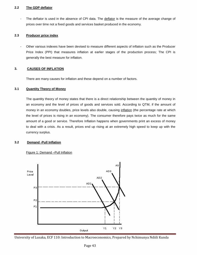
3.2 Demand -Pull Inflation
Figure 1: Demand –Pull Inflation

University of Lusaka, ECF 110: Introduction to Macroeconomics, Prepared by Nchimunya Ndiili Kunda Page 44
Demand-pull inflation happens where there is 'too much money chasing too few goods'. Excessive
growth in demand literally pulls prices up. Demand-pull inflation is asserted to arise when aggregate
demand in an economy outpaces aggregate supply. It involves inflation rising as real gross domestic
product rises and unemployment falls. This is commonly described as "too much money chasing too few
goods". More accurately, it should be described as involving "too much money spent chasing too few
goods", since only money that is spent on goods and services can cause inflation. This would not be
expected to persist over time due to increases in supply, unless the economy is already at a full
employment level.
Figure 1 shows the demand pull inflation where as more firms will employ people, the more people are
employed, and the higher aggregate demand will become. This greater demand will make firms employ
more people in order to increase output . Due to capacity constraints, this increase in output will
eventually become so small that the price of the good will rise. At first, unemployment will go down,
shifting AD1 to AD2, which increases Y by (Y2 - Y1). This increase in demand means more workers are
needed, and then AD will be shifted from AD2 to AD3, but this time much less is produced than in the
previous shift, but the price level has risen from P2 to P3, a much higher increase in price than in the
previous shift. This increase in price is called inflation.
3.3 Cost - Push Inflation
Source: Saving .R. Thomas, 2006
Cost-push inflation is a type of inflation caused by substantial increases in the production costs,
which leads to an increase in the price of the final product in the cost of important goods or services
where no suitable alternative is available. For example, if raw materials increase in price, this leads to
University of Lusaka, ECF 110: Introduction to Macroeconomics, Prepared by Nchimunya Ndiili Kunda Page 45
the cost of production increasing, which in turn leads to the company increasing prices to maintain
steady profits.
Monetarist economists such as Milton Friedman argue against the concept of cost-push inflation
because increases in the cost of goods and services do not lead to inflation without the government and
its central bank cooperating in increasing the money supply. The argument is that if the money supply is
constant, increases in the cost of a good or service will decrease the money available for other goods
and services, and therefore the price of some those goods will fall and offset the rise in price of those
goods whose prices have increased.
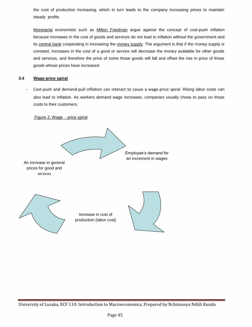
3.4 Wage-price spiral
- Cost-push and demand-pull inflation can interact to cause a wage-price spiral. Rising labor costs can
also lead to inflation. As workers demand wage increases, companies usually chose to pass on those
costs to their customers.
Figure 2; Wage - price spiral
Employee‘s demand for
an increment in wages
Increase in cost of
production (labor cost)
An increase in general
prices for good and
services

University of Lusaka, ECF 110: Introduction to Macroeconomics, Prepared by Nchimunya Ndiili Kunda Page 46
3.5 International lending and debts
- Inflation can also be caused by international lending and national debts. As nations borrow money, they
have to deal with interests, which in the end cause prices to rise as a way of keeping up with their debts.
A deep drop of the exchange rate can also result in inflation, as governments will have to deal with
differences in the import/export level.
3.6 Increase in fuel prices
- Finally, inflation can be caused by federal taxes put on consumer products such as fuel. As the taxes
rise, suppliers often pass on the burden to the consumer; the catch, however, is that once prices have
increased, they rarely go back, even if the taxes are later reduced. Wars are often cause for inflation, as
governments must both recoup the money spent and repay the funds borrowed from the central bank.
A situation that has been often cited of this was the oil crisis of the 1970s, which some economists see
as a major cause of the inflation experienced in the Western world in that decade. It is argued that this
inflation resulted from increases in the cost of petroleum imposed by the member states of OPEC. Since
petroleum is so important to industrialised economies, a large increase in its price can lead to the
increase in the price of most products, raising the inflation rate. This can raise the normal or built-in
inflation rate, reflecting adaptive expectations and the price/wage spiral, so that a supply shock can have
persistent effects
Note that war often affects everything from international trading to labor costs to product demand, so in
the end it always produces a rise in prices.
4. EFFECTS OF INFLATION
- Inflation affects different groups differently. Since the beginning of the 1980s, inflation has superseded
unemployment as the principal economic target for the government. The principal reason for switching
was because of the costs of inflation to the economy, and because they felt that if they could get low and
stable inflation, full employment would naturally follow. The seriousness of the costs of inflation depends
mainly on whether it is anticipated (expected) or unanticipated
4.1 Anticipated inflation
If people anticipate the inflation, then the effects will be less, as they will build these expectations into
their behavior. Nevertheless, there will be costs for firms who have to keep changing their prices. These
are called 'menu costs'.
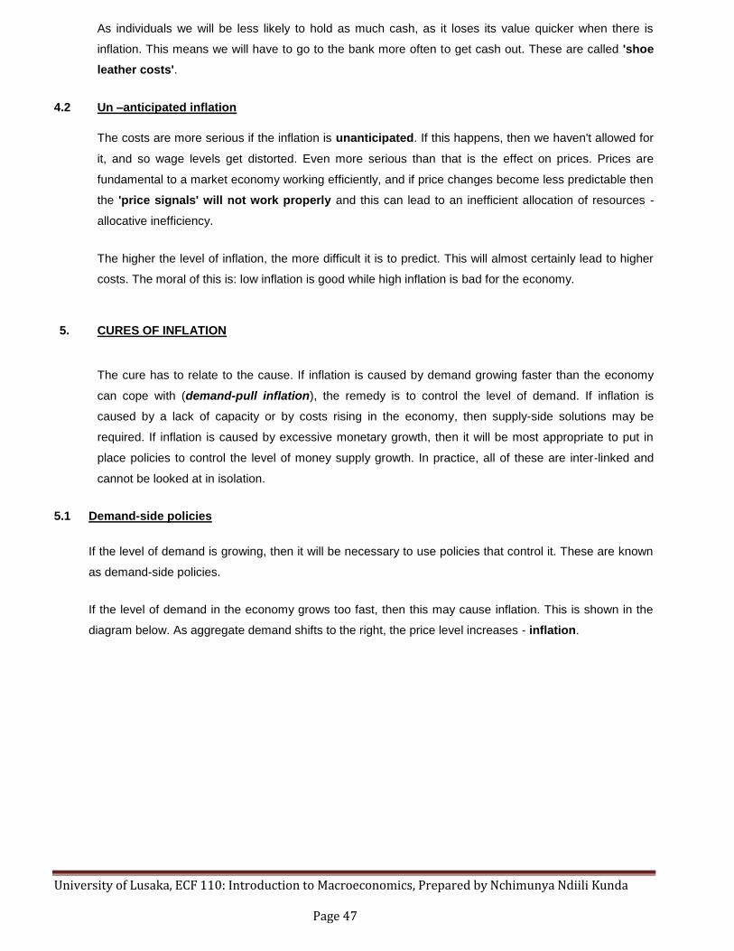
University of Lusaka, ECF 110: Introduction to Macroeconomics, Prepared by Nchimunya Ndiili Kunda Page 47
As individuals we will be less likely to hold as much cash, as it loses its value quicker when there is
inflation. This means we will have to go to the bank more often to get cash out. These are called 'shoe
leather costs'.
4.2 Un –anticipated inflation
The costs are more serious if the inflation is unanticipated. If this happens, then we haven't allowed for
it, and so wage levels get distorted. Even more serious than that is the effect on prices. Prices are
fundamental to a market economy working efficiently, and if price changes become less predictable then
the 'price signals' will not work properly and this can lead to an inefficient allocation of resources -
allocative inefficiency.
The higher the level of inflation, the more difficult it is to predict. This will almost certainly lead to higher
costs. The moral of this is: low inflation is good while high inflation is bad for the economy.
5. CURES OF INFLATION
The cure has to relate to the cause. If inflation is caused by demand growing faster than the economy
can cope with (demand-pull inflation), the remedy is to control the level of demand. If inflation is
caused by a lack of capacity or by costs rising in the economy, then supply-side solutions may be
required. If inflation is caused by excessive monetary growth, then it will be most appropriate to put in
place policies to control the level of money supply growth. In practice, all of these are inter-linked and
cannot be looked at in isolation.
5.1 Demand-side policies
If the level of demand is growing, then it will be necessary to use policies that control it. These are known
as demand-side policies.
If the level of demand in the economy grows too fast, then this may cause inflation. This is shown in the
diagram below. As aggregate demand shifts to the right, the price level increases - inflation.
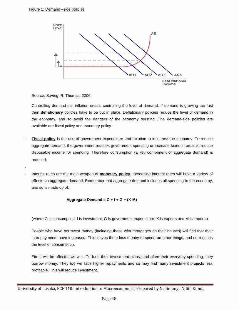
University of Lusaka, ECF 110: Introduction to Macroeconomics, Prepared by Nchimunya Ndiili Kunda Page 48
Figure 1: Demand –side policies
Source: Saving .R. Thomas, 2006
Controlling demand-pull inflation entails controlling the level of demand. If demand is growing too fast
then deflationary policies have to be put in place. Deflationary policies reduce the level of demand in
the economy, and so avoid the dangers of the economy bursting .The demand-side policies are
available are fiscal policy and monetary policy.
- Fiscal policy is the use of government expenditure and taxation to influence the economy. To reduce
aggregate demand, the government reduces government spending or increase taxes in order to reduce
disposable income for spending. Therefore consumption (a key component of aggregate demand) is
reduced.
-
- Interest rates are the main weapon of monetary policy. Increasing interest rates will have a variety of
effects on aggregate demand. Remember that aggregate demand includes all spending in the economy,
and so is made up of:
Aggregate Demand = C + I + G + (X-M)
(where C is consumption, I is investment, G is government expenditure, X is exports and M is imports)
People who have borrowed money (including those with mortgages on their houses) will find that their
loan payments have increased. This leaves them less money to spend on other things, and so reduces
the level of consumption.
Firms will be affected as well. To fund their investment plans, and often their everyday spending, they
borrow money. They too will face higher repayments and so may find many investment projects less
profitable. This will reduce investment.

University of Lusaka, ECF 110: Introduction to Macroeconomics, Prepared by Nchimunya Ndiili Kunda Page 49
Governments are also borrowers because they have to pay interest on the National Debt. An increase in
interest rates will raise the cost to them of servicing that debt. This will lead to a trade-off with other
spending .The government may have to cut spending on some other public service.
Higher interest rates may attract more overseas investment into the UK. This will lead to an increased
demand for sterling and may lead to an appreciation in the exchange rate. This could adversely affect
exports and lead to a further fall in aggregate demand.
5.2 Supply-side policies
- The economy can cope with increasing demand if the capacity of the economy grows fast enough.
Demand-pull inflation only happens when aggregate demand grows faster than the ability of the economy
to produce the goods. Therefore, if we can boost the capacity of the economy we may help to avoid
inflationary problems. Supply-side policies are policies that are aimed at doing this.
- Supply-side policies are aimed at making markets work better and removing possible market
imperfections. They could include:
Improved education and training
Reducing the power of trade unions to increase the flexibility of wage-setting
Reducing taxes to encourage investment and risk-taking
Reducing the level of tax to motivate people to work harder
Removing unnecessary regulations from markets that may hinder efficiency and innovation
The effect of these policies should be to shift the aggregate supply curve to the right. This is illustrated in
the diagram below. The economy clearly has a greater capacity to produce and can cope with a higher
level of aggregate demand before there is any increase in the price level.
Figure 2: Supply –side policies
Source: Saving .R. Thomas, 2006

University of Lusaka, ECF 110: Introduction to Macroeconomics, Prepared by Nchimunya Ndiili Kunda Page 50
5.3 Monetary and other targets
- Targets are set for various variables to help set policy. Recall that low and stable inflation is important to
create a healthy environment for business and the economy to prosper. The low inflation is given a target
in order to set policy appropriately.
- An inflation target is known as a final target. A target is set for the variable that is being controlled in this
instant the target is inflation. Most countries have an inflation target. For example, The UK inflation target is
2%, Australia is 3% and Zambia ‗ ‗s target is between 4% - 8% in 2010.
- It is generally reckoned that monetary policy changes can take up to two years to have their full effect, and
so a target also needs to be set for future inflation on the basis of forecasts for inflation.
- An intermediate target is a target set for a variable that affects the one that you are trying to control. In the
case of inflation, you could set targets for the level of money supply growth or perhaps for the exchange
rate. Both of these can act as an indicator of possible inflationary problems and help with setting policy.
5.4 Control of the money supply
The quantity theory of money suggests that control of the money supply will help in the fight against
inflation. The remedy is to use inflation target and interest rates to influence money supply growth
indirectly. However, there are various alternative techniques for controlling the money supply that have
been suggested over the years such as monetary base control, direct controls on lending and reserve
requirements.
5.4.1 Monetary base control
Banks are only able to lend to people and firms if they have enough liquid money available to meet their
liabilities. This is because the more they lend, the more money is required in the system. So, they have to
have more than enough cash available to handle all requests for cash at a given time. After all you
wouldn't be very happy if you turned up at your cash machine and it just said 'sorry'! This liquid money is
referred to as 'base money'. The theory of monetary base control is that if you control the amount of base
money available, you will limit the amount the banks can lend, and therefore limit the growth of the money
supply.
5.4.2 Direct controls on lending
Direct controls are regulations and requirements imposed on the banks and other financial institutions.
They may take various forms, but usually set limits on the amounts the banks can lend. They are also
often termed credit controls. These methods were dropped as the complexity and sophistication of the
financial system increased. It would now be very difficult to use them, and there is little will to use them
anyway. This is because they introduce all sorts of rigidities and reduce the amount of competition in
financial markets.
University of Lusaka, ECF 110: Introduction to Macroeconomics, Prepared by Nchimunya Ndiili Kunda Page 51
5.4.3 Reserve requirements
Banks have to place a proportion of their liabilities as a reserve requirement with the central bank. These
will often be non-interest bearing (pay no interest). The central bank could then use this reserve
requirement to influence how much the banks could lend. If they raise the reserve requirement, then the
banks would have to transfer money to the central bank and have less cash available to draw on when
people wanted it. This would limit the amount they could lend as they would not be able to afford to
generate new deposits. This would slow down the rate of growth of the money supply. Lowering the
reserve requirement would have the opposite effect and would enable the banks to expand their deposits,
increasing money supply growth.

University of Lusaka, ECF 110: Introduction to Macroeconomics, Prepared by Nchimunya Ndiili Kunda Page 52
UNIT: 8
TOPIC: UNEMPLOYMNET
LEARNING OBJECTIVE:
At the end of the lesson, students must be conversant of the different types of unemployment and
competent explain the causes, consequences and cures of unemployment. Students must know the
policies to implement in order to control high unemployment and achieve a desirable unemployment
rate .
SUB- TOPICS:
- Defining ‗full‘ employment
- Types of unemployment
- Measures of Unemployment
-Costs of unemployment
o Economic costs of unemployment
o Social costs of unemployment
- Inflation and unemployment (Phillips curve)
o The original Philips curve
o The critics of the Philips curve
o The expected augmented Philips curve
1. DEFINING ‘FULL’ EMPLOYMEN
- This is when all available labor resources are being used in the most economically efficient way. Full
employment embodies the highest amount of skilled and unskilled labor that could be employed within
an economy at any given time. When the economy is said to be at full employment, it is at its natural rate
of unemployment ( Begg .D, 2005)
1.1 Natural rate of unemployment
- This is the lowest rate of unemployment that an economy can sustain over the long run. Keynesians
believe that a government can lower the rate of unemployment (i.e. employ more people) if it were willing
to accept a higher level of inflation (the idea behind the Phillips Curve). However, critics of this say that
the effect is temporary and that unemployment would bounce back up but inflation would stay high.
Thus, the natural, or equilibrium, rate is the lowest level of unemployment at which inflation remains
stable. Also known as the "non-accelerating inflation rate of unemployment" (NAIRU).

University of Lusaka, ECF 110: Introduction to Macroeconomics, Prepared by Nchimunya Ndiili Kunda Page 53
1.2 Unemployment
- Unemployment is the number of people without jobs out of the labor force. It is an economic condition
where an individual or individuals seeking jobs remain un-hired. The level of unemployment differs with
economic conditions and other market forces. Basically there are five types of unemployment namely
frictional unemployment, structural unemployment, cyclical unemployment, classical unemployment and
seasonal unemployment.
2. TYPES OF UNEMPLOYMENT
2.1 Frictional Unemployment
- Frictional unemployment is the amount of unemployment that results from workers who are in between
jobs, but are still in the labor force. This unemployment occurs when an individual is out of his current
job and looking for another job. The time period of shifting between two jobs is known as frictional
unemployment. Frictional unemployment is a temporary condition. Many economists have estimated the
amount of frictional unemployment, with the number ranging from 2-7% of the labor force.
-
- Frictional unemployment is also a term used to describe unemployment that results from difficulties in matching
qualified workers with new jobs. Many qualified workers seeking work are not able to find new jobs right away,
usually because of a lack of complete information about new job openings. While it is likely that qualified workers will
soon be matched with new jobs, these workers are considered frictionally unemployed during the time that they
spend searching for their new jobs.
2.2 Structural Unemployment
- This is unemployment resulting from changes in the basic composition of the economy. These changes
simultaneously open new positions for trained workers. An example of structural unemployment is the
technological revolution. Computers may have eliminated jobs, but they also opened up new positions
for those who have the skills to operate the computers. Structural unemployment occurs due to the
structural changes within an economy.
- This type of unemployment occurs when there is a mismatch of skilled workers in the labor market.
Some of the causes of the structural unemployment are geographical immobility (difficulty in moving to a
new work location), occupational immobility (difficulty in learning a new skill) and technological change
(introduction of new techniques and technologies that need less labor force). Structural unemployment
depends on the growth rate of an economy and also on the structure of an industry.

University of Lusaka, ECF 110: Introduction to Macroeconomics, Prepared by Nchimunya Ndiili Kunda Page 54
- Structural unemployment results from structural changes in the economy that cause workers to lose
jobs. The same structural changes also prevent these workers from obtaining new jobs. Structurally
unemployed workers are not qualified for the new job openings that are available, mainly because they
lack the education or training needed for the new jobs. Consequently, the structurally unemployed tend
to be out of work for long periods of time, usually they learn the skills of the new jobs or until they decide
to relocate.
2.3 Cyclical unemployment
- This is unemployment that relates to the cyclical trends in growth and production that occur within the
business cycle. When business cycles are at their peak, cyclical unemployment will be low because total
economic output is being maximized. When economic output falls, as measured by the gross domestic
product (GDP), the business cycle is low and cyclical unemployment will rise. The aggregate demand for
goods and services decrease and demand for labor decreases.
-
- Economists describe cyclical unemployment as the result of businesses not having enough demand for
labor to employ all those who are looking for work. The lack of employer demand comes from a lack of
spending and consumption in the overall economy.
2.4 Seasonal unemployment
- This is unemployment that occurs due to the seasonal nature of the job is known as seasonal
unemployment. The industries that are affected by seasonal unemployment are hospitality industry,
tourism industries, fruit picking and catering industries.
2.5 Classical unemployment
- Classical unemployment is also known as the real wage unemployment or disequilibrium unemployment.
This type of unemployment occurs when trade unions and labor organization bargain for higher wages,
which leads to fall in the demand for labor.
3. MEASURING UNEMPLOYMENT
- The unemployment rate measures the percentage of the total civilian labor force that are currently
unemployed. The formula for the unemployment rate is given by
- The civilian labor force consists of all civilians (non-military personnel), 16 years of age or older,
who are willing to work and are not incarcerated. The number of people unemployed is determined
according to certain criteria. In the U.S., an unemployed person is a member of the civilian labor
force who is currently available for work and who has worked less than one hour per week for pay
or profit.

University of Lusaka, ECF 110: Introduction to Macroeconomics, Prepared by Nchimunya Ndiili Kunda Page 55
- Furthermore, an unemployed worker must have been actively searching for work during the past
month. Workers who are not actively searching for work, referred to as discouraged workers, are
not considered a part of the civilian labor force and therefore are not counted among the
unemployed.
5 . C O S T S O F U N E M P L O Y M E N T
- Most economists agree that high levels of unemployment are costly not only to the individuals and
families directly affected, but also to local and regional economies and the economy as a whole. We can
make a distinction between the economic costs arising from people out of work and the social costs
that often result.
5.1 Economic Costs
- Lost output of goods and services
Unemployment causes a waste of scarce economic resources and reduces the long run growth
potential of the economy. An economy with high unemployment is producing within its production
possibility frontier. The hours that the unemployed do not work can never be recovered.
Source; Poole. H, 2000
But if unemployment can be reduced, total national output can rise leading to an improvement in
economic welfare.

University of Lusaka, ECF 110: Introduction to Macroeconomics, Prepared by Nchimunya Ndiili Kunda Page 56
- Fiscal costs to the government
High unemployment has an impact on government expenditure, taxation and the level of government
borrowing each year. An increase in unemployment results in higher benefit payments and lower tax
revenues. When individuals are unemployed, not only do they receive benefits but also pay no income
tax. As they are spending less they contribute less to the government in indirect taxes.
This rise in government spending along with the fall in tax revenues may result in a higher government
borrowing requirement (known as a public sector net cash requirement)
- Deadweight loss of investment in human capital
Unemployment wastes some of the scarce resources used in training workers. Furthermore, workers
who are unemployed for long periods become de-skilled as their skills become increasingly dated in a
rapidly changing job market. This reduces their chances of gaining employment in the future, which in
turn increases the economic burden on government and society. See the revision page on long term
unemployment
5.2 SOCIAL COSTS OF UNEMPLOYMENT
- Rising unemployment is linked to social and economic deprivation - there is some relationship
between rising unemployment and rising crime and worsening social dislocation (increased divorce,
worsening health and lower life expectancy).
-
- Areas of high unemployment will also see a decline in real income and spending together with a rising
scale of relative poverty and income inequality. As younger workers are more geographically mobile
than older employees, there is a risk that areas with above average unemployment will suffer from an
ageing potential workforce - making them less attractive as investment locations for new businesses.
5.3 The duration of unemployment affects the economic and social costs
- It is clear therefore that unemployment carries substantial economic and social costs. These costs are
greatest when long-term structural unemployment is high. Indeed many governments focus their labor
market policies on improving the employment prospects of the long-term unemployed.

University of Lusaka, ECF 110: Introduction to Macroeconomics, Prepared by Nchimunya Ndiili Kunda Page 57
6. INFLATION AND UNEMPLOYMENT
- The Phillips Curve shows the short-term trade-off between unemployment and inflation. The original
Phillips Curve has come under sustained attack – in particular from monetarist economists
6.1 Original Phillips Curve idea
- The originator of the Philips curve was AW Philips in 1958 .He plotted 95 years of data of UK wage
inflation against unemployment. It seemed to suggest a short-run trade-off between unemployment and
inflation. The theory behind this was fairly straightforward. Falling unemployment might cause rising
inflation and a fall in inflation might only be possible by allowing unemployment to rise. If the
Government wanted to reduce the unemployment rate, it could increase aggregate demand but,
although this might temporarily increase employment, it could also have inflationary implications in labor
and the product markets.
-
- The key to understanding this trade-off is to consider the possible inflationary effects in both labor and
product markets arising from an increase in national income, output and employment:
The labor market:
As unemployment falls, some labor shortages may occur where skilled labor is in short supply. This puts
extra pressure on wages to rise, and since wages are usually a high percentage of total costs,
prices may rise as firms pass on these costs to their customers.
Other factor markets:
Cost-push inflation can also come from rising demand for commodities such as oil, copper and
processed manufactured goods such as steel, concrete and glass. When an economy is booming, so
does demand for these components and raw materials.
Product markets:
Rising demand and output puts pressure on scarce resources and can lead to suppliers raising prices to
widen profit margins. The risk of rising prices is greatest when demand is out-stripping supply-capacity
leading to excess demand.
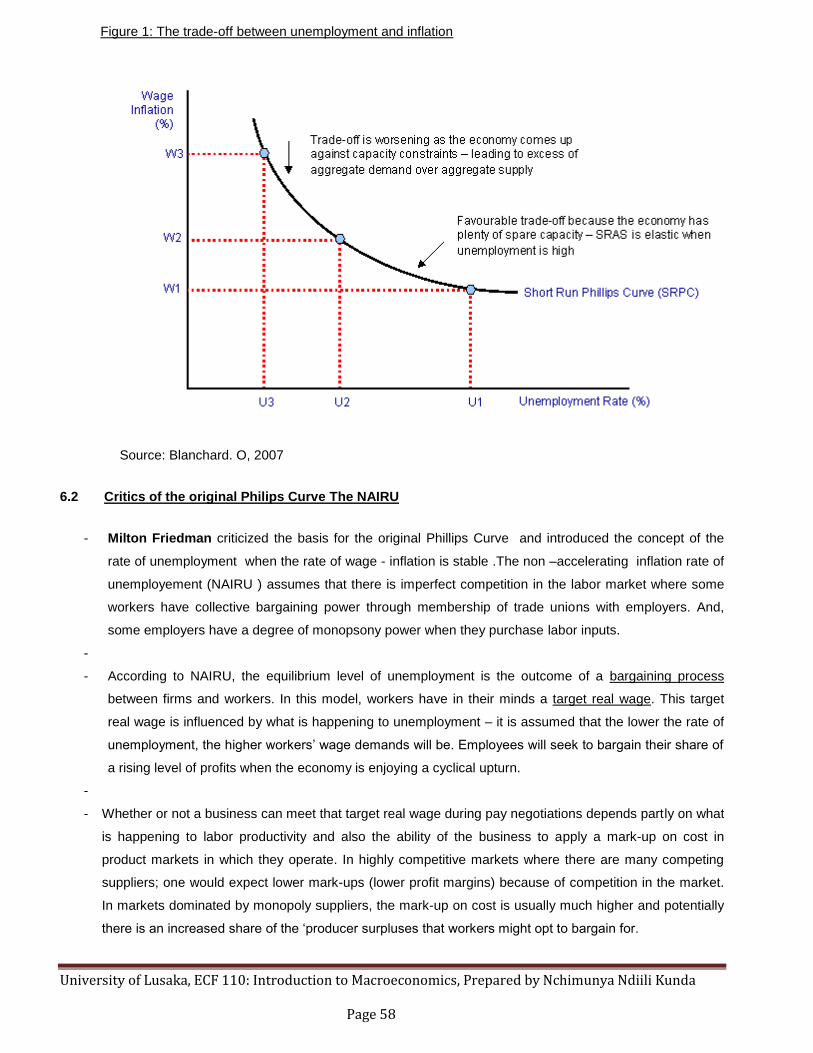
University of Lusaka, ECF 110: Introduction to Macroeconomics, Prepared by Nchimunya Ndiili Kunda Page 58
Figure 1: The trade-off between unemployment and inflation
Source: Blanchard. O, 2007
6.2 Critics of the original Philips Curve The NAIRU
- Milton Friedman criticized the basis for the original Phillips Curve and introduced the concept of the
rate of unemployment when the rate of wage - inflation is stable .The non –accelerating inflation rate of
unemployement (NAIRU ) assumes that there is imperfect competition in the labor market where some
workers have collective bargaining power through membership of trade unions with employers. And,
some employers have a degree of monopsony power when they purchase labor inputs.
-
- According to NAIRU, the equilibrium level of unemployment is the outcome of a bargaining process
between firms and workers. In this model, workers have in their minds a target real wage. This target
real wage is influenced by what is happening to unemployment – it is assumed that the lower the rate of
unemployment, the higher workers‘ wage demands will be. Employees will seek to bargain their share of
a rising level of profits when the economy is enjoying a cyclical upturn.
-
- Whether or not a business can meet that target real wage during pay negotiations depends partly on what
is happening to labor productivity and also the ability of the business to apply a mark-up on cost in
product markets in which they operate. In highly competitive markets where there are many competing
suppliers; one would expect lower mark-ups (lower profit margins) because of competition in the market.
In markets dominated by monopoly suppliers, the mark-up on cost is usually much higher and potentially
there is an increased share of the ‗producer surpluses that workers might opt to bargain for.

University of Lusaka, ECF 110: Introduction to Macroeconomics, Prepared by Nchimunya Ndiili Kunda Page 59
- If actual unemployment falls below the NAIRU, theory suggests that the balance of power in the labor
market tends to switch to employees rather than employers. The consequence can be that the economy
experiences acceleration in pay settlements and the growth of average earnings. Ceteris paribus, an
increase in wage inflation will cause a rise in cost-push inflationary pressure.
6.3 The expectations-augmented Phillips Curve ( Modern Philips Curve)
- The original Phillips Curve idea was subjected to fierce criticism from the Monetarist school among them
but that in the long run, the Phillips Curve was vertical and that there was no trade-off between
unemployment and inflation.
-
- He argued that each short run Phillips Curve was drawn on the assumption of a given expected rate of
inflation. So if there were an increase in inflation caused by a large monetary expansion and this had the
effect of driving inflationary expectations higher, then this would cause an upward shift in the short run
Phillips Curve.
Friedman introduced the idea of adaptive expectations –
This is illustrated in the next diagram – inflation expectations are higher for SPRC2. The result may be
that higher unemployment is required to keep inflation at a certain target level.

University of Lusaka, ECF 110: Introduction to Macroeconomics, Prepared by Nchimunya Ndiili Kunda Page 60
Figure 2: Expected Augmented Philips Curve
Source: Blanchard. O, 2007
The natural rate of unemployment is the unemployment rate such that the real wage chosen in wage
setting is equal to the real wage implied by price setting.
The expectations-augmented Phillips Curve argues that attempts by the government to reduce
unemployment below the natural rate of unemployment by boosting aggregate demand will have little
success in the long run. The effect is merely to create higher inflation and with it an increase in inflation
expectations. The Monetarist school believes that inflation is best controlled through tight control of
money and credit. Credible policies to keep on top of inflation can also have the beneficial effect of
reducing inflation expectations – causing a downward shift in the Phillips Curve.
- The monetarist view is that attempts to boost AD to achieve faster growth and lower unemployment have
only a temporary effect on jobs. Friedman argued that a government could not permanently drive
unemployment down below the NAIRU – the result would be higher inflation which in turn would
eventually bring about a return to higher unemployment but with inflation expectations increased along
the way.
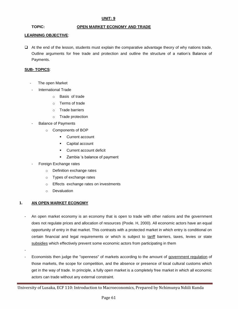
University of Lusaka, ECF 110: Introduction to Macroeconomics, Prepared by Nchimunya Ndiili Kunda Page 61
UNIT: 9
TOPIC: OPEN MARKET ECONOMY AND TRADE
LEARNING OBJECTIVE:
At the end of the lesson, students must explain the comparative advantage theory of why nations trade,
Outline arguments for free trade and protection and outline the structure of a nation‘s Balance of
Payments.
SUB- TOPICS:
- The open Market
- International Trade
o Basis of trade
o Terms of trade
o Trade barriers
o Trade protection
- Balance of Payments
o Components of BOP
Current account
Capital account
Current account deficit
Zambia ‗s balance of payment
- Foreign Exchange rates
o Definition exchange rates
o Types of exchange rates
o Effects exchange rates on investments
o Devaluation
1. AN OPEN MARKET ECONOMY
- An open market economy is an economy that is open to trade with other nations and the government
does not regulate prices and allocation of resources (Poole. H, 2000). All economic actors have an equal
opportunity of entry in that market. This contrasts with a protected market in which entry is conditional on
certain financial and legal requirements or which is subject to tariff barriers, taxes, levies or state
subsidies which effectively prevent some economic actors from participating in them
-
- Economists then judge the "openness" of markets according to the amount of government regulation of
those markets, the scope for competition, and the absence or presence of local cultural customs which
get in the way of trade. In principle, a fully open market is a completely free market in which all economic
actors can trade without any external constraint.

University of Lusaka, ECF 110: Introduction to Macroeconomics, Prepared by Nchimunya Ndiili Kunda Page 62
-
- In reality, few markets exist which are open to that extent, since they usually cannot operate without an
enforceable legal framework for trade which guarantees security of property, the fulfillment of contractual
obligations associated with transactions, and the prevention of cheating. In response to this type of
criticism, the concept of open market is often redefined to mean a situation of free competition, and the
inability to participate is explained as a lack of competitiveness.
2. INTERNATIONAL TRADE
- International trade allows a country to consume a combination of goods and services that exceeds its
production possibilities curve. The theory of international trade assumes:
• There are two countries
• Each produces two goods, but initially there is no trade.
The following table shows the possible production of two goods in two economies
Table 1: Production of wine and salt
Good Spain Portugal
Wine 15 40
Salt 30 40
Source: Layton Robinson & Tucker, 2009
Figure 1: Pre –trade production possibility frontier
Wine
40 Portugal
15 Spain
30 40 Salt
Source: Layton Robinson & Tucker, 2009

University of Lusaka, ECF 110: Introduction to Macroeconomics, Prepared by Nchimunya Ndiili Kunda Page 63
2.1 Basis of Trade
2.1.1 Adam Smith – Absolute Advantage
According to Adam Smith Model of absolute advantage in labor, the country with the relatively higher
labor productivity in a commodity should completely specialize and export that commodity and import the
commodity where it has relatively lower labor productivity.
Absolute advantage of the production of a commodity is represented on the diagram by a higher
intercept (indicates higher labor productivity).
Figure 2: Absolute advantage production possibility frontier
Wine
40 Portugal
15 Spain
30 40 Salt
Source: Layton Robinson & Tucker, 2009
Portugal has a higher intercept indicating that it has higher labor productivity in the production of wine.
Based on absolute advantage, Portugal has comparative advantage in the production of wine.
2.1.2 Ricardian model – Comparative Advantage
The country with the relatively lower opportunity cost in the production of a commodity should completely
specialize and export that commodity. It should, at the same time, import the commodity which it has a
relatively higher opportunity cost. The country should produce the commodity in which it has the greatest
comparative advantage or countries should do what they do best
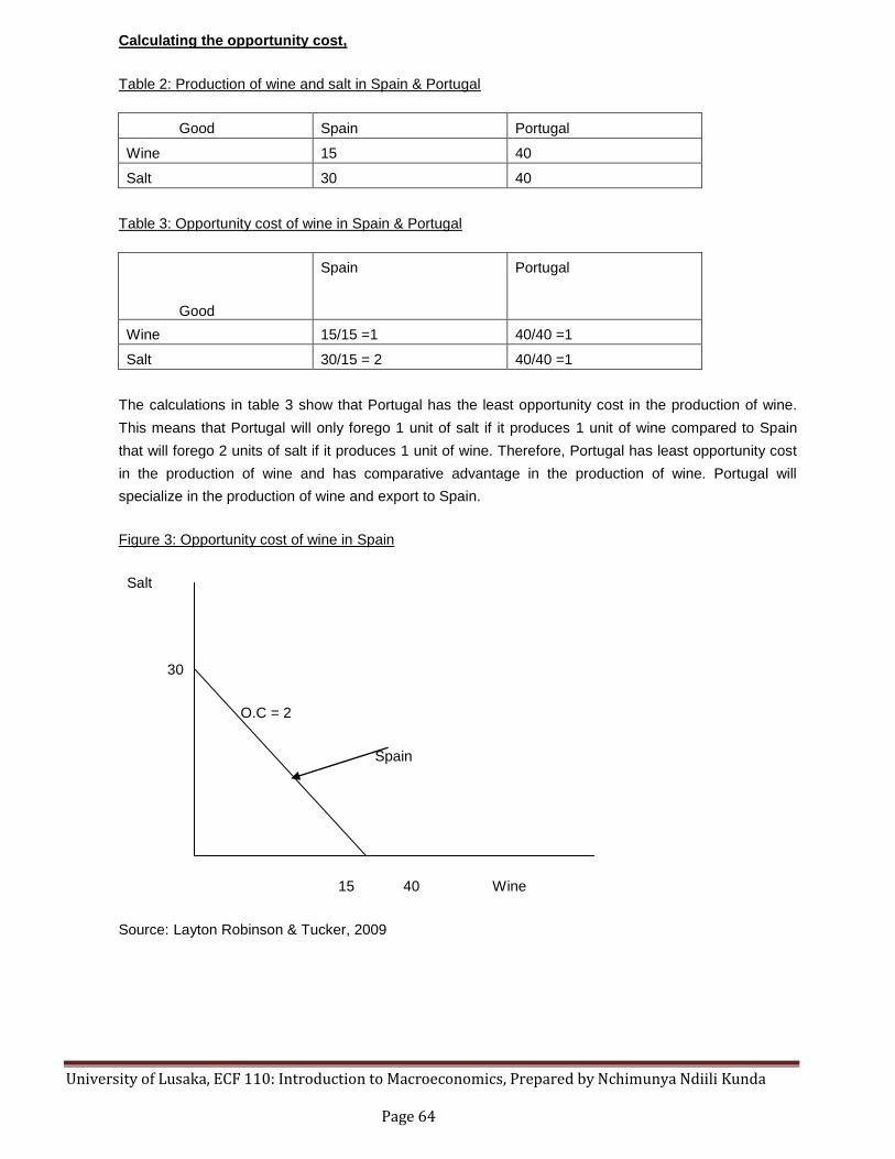
University of Lusaka, ECF 110: Introduction to Macroeconomics, Prepared by Nchimunya Ndiili Kunda Page 64
Calculating the opportunity cost,
Table 2: Production of wine and salt in Spain & Portugal
Good Spain Portugal
Wine 15 40
Salt 30 40
Table 3: Opportunity cost of wine in Spain & Portugal
Good
Spain Portugal
Wine 15/15 =1 40/40 =1
Salt 30/15 = 2 40/40 =1
The calculations in table 3 show that Portugal has the least opportunity cost in the production of wine.
This means that Portugal will only forego 1 unit of salt if it produces 1 unit of wine compared to Spain
that will forego 2 units of salt if it produces 1 unit of wine. Therefore, Portugal has least opportunity cost
in the production of wine and has comparative advantage in the production of wine. Portugal will
specialize in the production of wine and export to Spain.
Figure 3: Opportunity cost of wine in Spain
Salt
30
O.C = 2
Spain
15 40 Wine
Source: Layton Robinson & Tucker, 2009
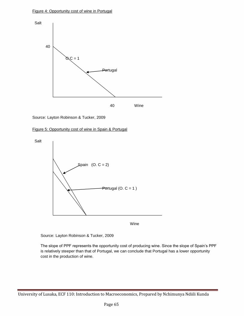
University of Lusaka, ECF 110: Introduction to Macroeconomics, Prepared by Nchimunya Ndiili Kunda Page 65
Figure 4: Opportunity cost of wine in Portugal
Salt
40
O.C = 1
Portugal
40 Wine
Source: Layton Robinson & Tucker, 2009
Figure 5: Opportunity cost of wine in Spain & Portugal
Salt
Spain (O. C = 2)
Portugal (O. C = 1 )
Wine
Source: Layton Robinson & Tucker, 2009
The slope of PPF represents the opportunity cost of producing wine. Since the slope of Spain‘s PPF
is relatively steeper than that of Portugal, we can conclude that Portugal has a lower opportunity
cost in the production of wine.
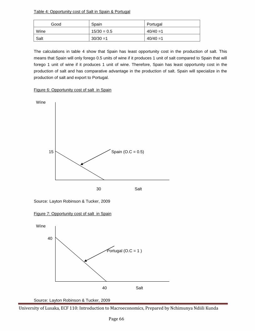
University of Lusaka, ECF 110: Introduction to Macroeconomics, Prepared by Nchimunya Ndiili Kunda Page 66
Table 4: Opportunity cost of Salt in Spain & Portugal
Good Spain Portugal
Wine 15/30 = 0.5 40/40 =1
Salt 30/30 =1 40/40 =1
The calculations in table 4 show that Spain has least opportunity cost in the production of salt. This
means that Spain will only forego 0.5 units of wine if it produces 1 unit of salt compared to Spain that will
forego 1 unit of wine if it produces 1 unit of wine. Therefore, Spain has least opportunity cost in the
production of salt and has comparative advantage in the production of salt. Spain will specialize in the
production of salt and export to Portugal.
Figure 6: Opportunity cost of salt in Spain
Wine
15 Spain (O.C = 0.5)
30 Salt
Source: Layton Robinson & Tucker, 2009
Figure 7: Opportunity cost of salt in Spain
Wine
40
Portugal (O.C = 1 )
40 Salt
Source: Layton Robinson & Tucker, 2009

University of Lusaka, ECF 110: Introduction to Macroeconomics, Prepared by Nchimunya Ndiili Kunda Page 67
Figure 8: Opportunity cost of salt in Spain & Portugal
Wine
Portugal (O.C = 1)
Spain (O.C = 0.5)
Salt
Source: Layton Robinson & Tucker, 2009
The slope of PPF represents the opportunity cost of producing salt. Since the slope of Portugal‘s PPF is
relatively steeper than that of Spain, we can conclude that Spain has a lower opportunity cost in the
production of salt.
2.2 Terms of trade
- Domestic opportunity costs (pre trade prices) set the limits to the single world price which will emerge
with trade. The world price is also known as international price ratio. Portugal will export wine, but only if
the price is at least 1 unit of salt (before trade it could already have 1 salt for every 1 wine it gave up).
Spain would be happy to pay up to 2 units of salt (Spain‘s pre trade cost). Any rate of exchange between
the domestic price ratios will be acceptable. Note this is not dollars, but opportunity costs.
Assume the final price is 1 wine for 1.5 salt. Portugal can now get 1.5 salt for every wine it chooses to
trade instead of the initial ( pre –trade) 1 wine for 1.5 salt.
2.3 Gains from Trade
A country gains more in trade compared to producing a product locally and consuming it locally. By
exporting a product where a country has least opportunity cost and importing a product where it has high
opportunity cost, a country will consume more of a high opportunity cost product through trade.
Lets say Portugal chooses to export 20 wine. How many units of salt can they get now?
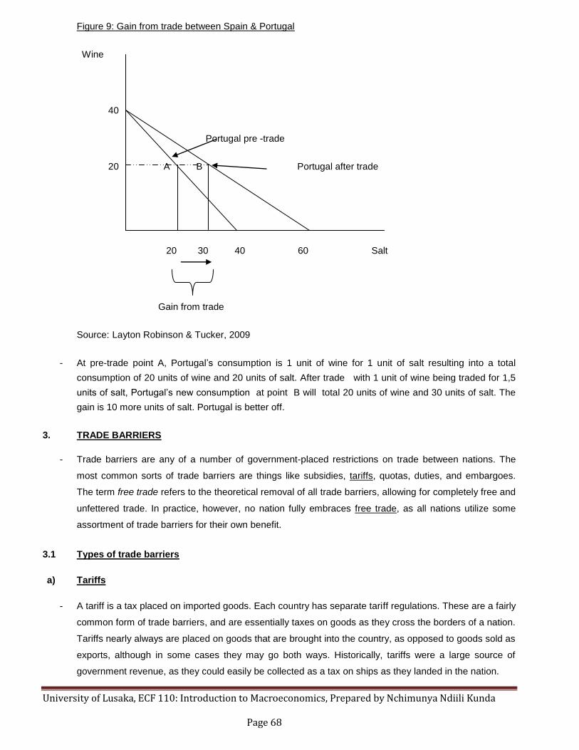
University of Lusaka, ECF 110: Introduction to Macroeconomics, Prepared by Nchimunya Ndiili Kunda Page 68
Figure 9: Gain from trade between Spain & Portugal
Wine
40
Portugal pre -trade
20 A B Portugal after trade
20 30 40 60 Salt
Gain from trade
Source: Layton Robinson & Tucker, 2009
- At pre-trade point A, Portugal‘s consumption is 1 unit of wine for 1 unit of salt resulting into a total
consumption of 20 units of wine and 20 units of salt. After trade with 1 unit of wine being traded for 1,5
units of salt, Portugal‘s new consumption at point B will total 20 units of wine and 30 units of salt. The
gain is 10 more units of salt. Portugal is better off.
3. TRADE BARRIERS
- Trade barriers are any of a number of government-placed restrictions on trade between nations. The
most common sorts of trade barriers are things like subsidies, tariffs, quotas, duties, and embargoes.
The term free trade refers to the theoretical removal of all trade barriers, allowing for completely free and
unfettered trade. In practice, however, no nation fully embraces free trade, as all nations utilize some
assortment of trade barriers for their own benefit.
3.1 Types of trade barriers
a) Tariffs
- A tariff is a tax placed on imported goods. Each country has separate tariff regulations. These are a fairly
common form of trade barriers, and are essentially taxes on goods as they cross the borders of a nation.
Tariffs nearly always are placed on goods that are brought into the country, as opposed to goods sold as
exports, although in some cases they may go both ways. Historically, tariffs were a large source of
government revenue, as they could easily be collected as a tax on ships as they landed in the nation.

University of Lusaka, ECF 110: Introduction to Macroeconomics, Prepared by Nchimunya Ndiili Kunda Page 69
The five main types of tariffs include revenue, advalorem, specific, prohibitive and protective.
Revenue Tariff: A revenue tariff increases government funds. For example, countries that do not grow
bananas may create a tariff on importing bananas. The government would then make money from
businesses that import bananas.
An ad valorem: tariff means that the tariff applies to a percentage of the import's value such as a set
number of cents on every dollar of value. A specific tariff, on the other hand, means that the tariff is not
concerned with the estimated value of the imported goods, but rather is based on specific amount of the
goods. A specific tariff may apply to the number of goods imported or to the weight, volume or other
measurement of the goods.
Prohibitive tariff: is one that is such as high cost that it keeps the item from being imported. A
protective tariff is used to raise the price of imported goods as a protective measure against the
competition from foreign markets. A higher tariff allows a local company to compete with foreign
competition.
Protective tariffs: can be advantageous as they can help foster the local economy, but sometimes they
can also make the price of the item so expensive that companies must charge more. For example, when
gas prices become too high, industries such as the trucking industry may have to charge retailers more
for delivering products. The retail industry then has to mark up their items to allow for their increased
transportation costs in order to make the same profit they once did. The end result is that consumers pay
more for the goods.
- Tariffs, like most trade barriers, may be imposed for different reasons. Some tariffs are placed simply to
earn money for the government. This might either be a flat fee on an item, or it might be based on the
market value of the item. Other tariffs exist as a form of protectionism, to make imported goods more
expensive than they might otherwise be, in order to protect domestic industries. For example, if a
country has a fairly high wage, and high labor standards, the cost of producing a single widget might be
around ten units. If a nearby country can produce a widget for three units, then imports of that country‘s
widgets could easily drive the domestic industry out of business. So the country might place a restrictive
tariff on widget imports, to make sure that domestic widgets always remained competitively priced, or
even to make it unfeasible for widgets to be imported at all.
b) Subsidies
- Subsidies are another of the common trade barriers, and are often placed to protect domestic industries.
Subsidies may actually be intended simply to make certain key goods affordable to citizens of the nation,
but the end result can still be to make imports non-competitive. Many food crops, for example, are
heavily subsidized, to ensure the citizenry has a constant supply of affordable food. Steel is also often
subsidized, to ensure a nation always has a domestic steel supply, which can be crucial during times of
war when normal shipping avenues may be cut off.

University of Lusaka, ECF 110: Introduction to Macroeconomics, Prepared by Nchimunya Ndiili Kunda Page 70
c) Embargo
- An embargo can be seen as the most extreme of the trade barriers. Embargoes basically prohibit the
import or export of anything with another country. This is often done as a form of punishment, or to try to
force the country to undergo radical change internally as a result of a weakened economic state.
Historically, the embargo was used as a war tactic, and so was often considered a declaration of war. In
modern times, however, although the most brutal of the trade barriers, it is usually not viewed as an act
of outright aggression, although a declaration of war is often accompanied by an embargo.
d) Quotas – a limit on the quantity of a good that may be imported.
4. TRADE PROTECTIONISM
- Protectionism is an economic policy which is meant to benefit domestic producers of goods and
services. In a nation with protectionist policies, domestic producers are insulated from competition
against foreign firms by a series of barriers to import. They may also be supported directly by the
government with the use of subsidies. The opposite of protectionism is free trade, in which goods are
freely permitted to cross borders. Many nations support free trade, and would prefer to see protectionist
economic policies barred altogether. Signatories to the General Agreement of Tariffs and Trade (GATT)
and members of the World Trade Organization (WTO), for example, are typically proponents of free
trade.
-
- The logic behind protectionism is that domestic industries may suffer when confronted with foreign
imports which are available at cheaper prices due to lower cost of labor, more readily available natural
resources, or foreign government subsidies which help the producers keep their costs low. By imposing
stiff import tariffs and quotas, a government can theoretically increase the market for domestic goods, by
essentially closing the market to foreign producers. This in turn is designed to benefit the domestic
economy.
-
- When restrictions on imports are accompanied by government subsidies to domestic companies and
government export subsidies to encourage exports of domestic products, protectionism is intended to
benefit domestic companies.
-
- Supporters of protectionism argue that it can help nascent industries by insulating them from the open
market until they are strong enough to function independently.
-
- Protectionism also theoretically protects domestic employment, by encouraging companies to hire
domestically, and it can be used to promote living wages and better benefits for employees. Proponents
point out that protectionism can also be used to pressure foreign nations to improve conditions for their
workers.
University of Lusaka, ECF 110: Introduction to Macroeconomics, Prepared by Nchimunya Ndiili Kunda Page 71
Negative effects of protectionism
- Protectionism leads to lack of competition. Domestic companies may have less interest in developing
innovative new products, sticking with old inventions and technologies. They may also face export
barriers, because foreign countries often respond to protectionism with protectionist policies of their own.
-
- Individual citizens can also suffer under protectionism, because they may find that prices for goods and
services become inflated. Without low-cost foreign competition, companies can afford to charge
whatever they like for their goods and services, and this means that consumers may pay prices which
are much higher than those paid by people in other regions of the world. They may also chafe at the lack
of innovation, or lobby for a greater freedom to choose between products.
5. FREE TRADE BODIES
- A number of free trade bodies exist in the world to try to curtail the use of trade barriers by nations. The
World Trade Organization is perhaps the widest reaching of these bodies, and it enforces strict rules
against member nations, restricting the acceptable use of things like tariffs. As a result, some countries
have begun using trade barriers that are not tariffs, but have similar effects. The European Union, for
example, does not allow the import of many genetically-modified organisms, which effectively bans the
vast majority of food imports from the United States. In recent years, groups like the WTO have begun to
look at these forms of trade barriers as well, and to strip them when possible.
5.1 World trade Organization
- According to the World Trade Organization (WTO), its goal is to help producers of goods and services,
exporters, and importers conduct their business. This international organization accomplishes this mainly
by helping countries establish and agree upon trade rules. Without such an organization, it is likely that
trade relations between foreign entities could be difficult, unfair, and inconsistent.
-
- The World Trade Organization was created in 1995 and has three official languages: French, English
and Spanish. The organization has hundreds of members around the globe, however, and aims to work
in the best interest of all of them. Most decisions made by the WTO are matters of consensus. This
means that all members agree upon them.
-
- A trade agreement usually contains both the rights and obligations of the agreeing parties. WTO
agreements can generally be divided into two categories. Multilateral agreements refer to those that all
World Trade Organization members have agreed to. Plurilateral agreements are those that only some
members have agreed to.
-
- Different countries tend to have different cultures. Many people in business realize that culture can be a
major factor in determining how affairs are conducted. Other factors such as previous experiences, both
good and bad, can determine the business decisions that are made. These are just two of many

University of Lusaka, ECF 110: Introduction to Macroeconomics, Prepared by Nchimunya Ndiili Kunda Page 72
examples of factors that could cause trade barriers or trade inconsistencies if such business
arrangements were left to the whim of individuals.
-
- One thing that the World Trade Organization aims to do is normalize trade. This means that certain
practices should be kept consistent. For example, the organization may secure agreements among trade
partners that prevent politics from playing a role in the initiation or rise of tariffs.
-
- In addition to easing trade transactions, the World Trade Organization also aims to eliminate
discrimination from international exchange. This can produce the dual benefits of allowing producers
access to foreign markets and allowing consumers access to foreign goods. This can also prevent
substantial economic growth for some while economic growth is unfairly or unethically inhibited for
others.
5.2 EUROPEAN UNION
- The European Union, or EU, is a collaborative effort between 27 European countries to form a mutually
beneficial economic and policy community. Since 1993, the EU has worked to increase economies and
spread human rights advances worldwide. The goals of the European Union include uniting Europe
toward common goals and providing aid to developing nations.
-
- After World War II, Europe was a fractured area, divided by political and cultural differences. Several
attempts to promote a regional governing body met with varying success, including the European Coal
and Steel Community and the European Community. Because of the power ideological and political
differences between Western and Eastern Europe, a true community could not be formed until after the
end of the Cold War
-
- In 1992, the Maastricht Treaty was signed by member nations, bringing the European Union into effect.
The treaty outlined three pillars of the union: European Communities, Common Foreign and Security
Policy, and Justice and Home Affairs. The treaty also made provisions to admit many of the nations of
Eastern Europe. In 2001, the Treaty of Nice further expanded provisions for new nations.
-
- To become a member of the European Union, a nation must be in conformance with a series of
standards called the Copenhagen criteria. These detail geographic and political necessities for member
nations. Included standards dictate human rights laws, democracy, protective law for minorities, and a
market economy. As of 2008, three states are candidates undergoing review: Turkey, Croatia, and the
Republic of Macedonia. Several other nations are identified as potential candidates for future admission,
including Albania and Serbia.
-
- One of the greatest achievements of the European Union is the establishment of a single market
economy. Between member nations, trade is largely unrestricted. While nations maintain separate laws
University of Lusaka, ECF 110: Introduction to Macroeconomics, Prepared by Nchimunya Ndiili Kunda Page 73
on taxation and trade standards, EU members agree to basic trade laws between their countries. Almost
all products created by one nation are legal for trade in all of the other countries.
-
- Most nations belonging to the EU have adopted a common currency, called the Euro. The Euro is
overseen by the European Central Bank, in an effort to promote all economies that incorporate the use
of the currency. As of 2008, 15 nations use the Euro, collectively called the Euro zone. Other EU
members must meet specific financial and economic standards before being allowed to adopt the
currency. Slovenia was the first of the countries from the 2004 expansion to meet euro criteria.

University of Lusaka, ECF 110: Introduction to Macroeconomics, Prepared by Nchimunya Ndiili Kunda Page 74
.6. THE BALANCE OF PAYMENTS
The balance of payments is a summary of international transactions between one country and others
over a period of time. This summary records the nature and value of inflows and outflows of goods,
services and financial assets .The balance of payments comprises of the current account and the capital
account.
6.1 The current account
The current account records trade in goods and services. It consists of balances on
o merchandise trade (goods) that is exports less imports
o services (e.g. tourism, education)
o income (e.g. dividends and interest payments)
o transfers.
6.2 The capital account
The capital account records dollar payments flows of purchases of foreign assets by Australians, and of
domestic assets by foreigners. The assets referred to are ‗investment assets such as bonds, securities,
property, shares
Note that any income flowing from the ownership of these assets is recorded as income in the current
account.
Current and capital account offset each other.The current and capital accounts should balance (any
difference is a measurement error).This is because any deficit on the current account is financed by a
surplus on the capital account – foreigners accommodate additional current expenditure by becoming
investors in the country.
6.3 The current account deficit
- Most countries have experienced a current account deficit (CAD) in every year since 1960.This means
that countries spend more than the income they generate, so foreigners are accumulating domestic
assets.
-
- The CAD is not likely to prove a problem provided overseas funds are used to finance investment goods
which earn income in the future.
-
- There has been a significant rise in foreign liabilities and debt over the past 25 years in most developing
countries. Much of this is explained by financial deregulation and the freeing up of international financial
markets over the last 20 years in direct investment, portfolio investment
-
- It is important to note that the amount of foreign liabilities is not a concern provided the debt can be
serviced (just like a housing loan). This is more likely if liabilities have been incurred to generate income.
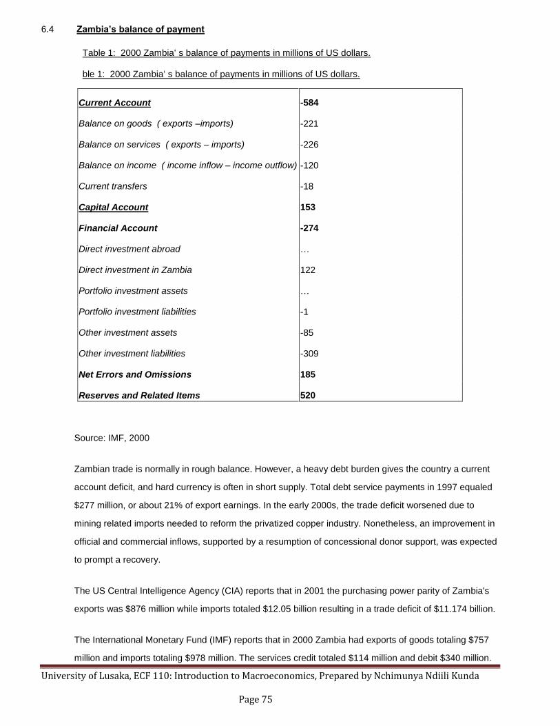
University of Lusaka, ECF 110: Introduction to Macroeconomics, Prepared by Nchimunya Ndiili Kunda Page 75
6.4 Zambia’s balanc of paym nt
Table 1: 2000 Zambia‗ s balance of payments in millions of US dollars.
ble 1: 2000 Zambia‗ s balance of payments in millions of US dollars.
Source: IMF, 2000
Zambian trade is normally in rough balance. However, a heavy debt burden gives the country a current
account deficit, and hard currency is often in short supply. Total debt service payments in 1997 equaled
$277 million, or about 21% of export earnings. In the early 2000s, the trade deficit worsened due to
mining related imports needed to reform the privatized copper industry. Nonetheless, an improvement in
official and commercial inflows, supported by a resumption of concessional donor support, was expected
to prompt a recovery.
The US Central Intelligence Agency (CIA) reports that in 2001 the purchasing power parity of Zambia's
exports was $876 million while imports totaled $12.05 billion resulting in a trade deficit of $11.174 billion.
The International Monetary Fund (IMF) reports that in 2000 Zambia had exports of goods totaling $757
million and imports totaling $978 million. The services credit totaled $114 million and debit $340 million.
Current Account -584
Balance on goods ( exports –imports) -221
Balance on services ( exports – imports) -226
Balance on income ( income inflow – income outflow) -120
Current transfers -18
Capital Account 153
Financial Account -274
Direct investment abroad …
Direct investment in Zambia 122
Portfolio investment assets …
Portfolio investment liabilities -1
Other investment assets -85
Other investment liabilities -309
Net Errors and Omissions 185
Reserves and Related Items 520

University of Lusaka, ECF 110: Introduction to Macroeconomics, Prepared by Nchimunya Ndiili Kunda Page 76
7. EXCHANGE RATES
- The exchange rate is the price of one currency expressed in terms of another currency. It is also defined
as the price of the domestic currency for one unit of a foreign currency.
For example if ZMK 5000 buys $1 dollars, the exchange rate is expressed as:
ZMK 5000 = 5000.
$1
7.1 TYPES OF EXCHANGE RATES
a) Nominal exchange rate
The nominal exchange rate ε is defined as the number of units of the domestic currency that can
purchase a unit of a given foreign currency.
ε = ZMK 5000 = 5000.
$1
Where :ZMK 5000 is also referred to as the price currency or term currency
: $1 is also reffered to as the price commodity currency or base currency
A decrease in this variable is termed nominal appreciation of the currency. (Under the fixed exchange
rate regime, a downward adjustment of the rate ε is termed revaluation.) An increase in this variable is
termed nominal depreciation of the currency. (Under the fixed exchange rate regime, an upward
adjustment of the rate ε is called devaluation.)
Nominal exchange rates are established on currency financial markets called "forex markets", which
are similar to stock exchange markets. Rates are usually established in continuous quotation, with
newspaper reporting daily quotation (as average or finishing quotation in the trade day on a specific
market). Central bank may also fix the nominal exchange rate. In most parts of the world, the market
convention that determines which is the base currency and which is the term currency is in the order :
EUR – GBP – AUD – NZD – USD – others.
Quotes using a country's home currency as the price currency (e.g., EUR 0.735342 = USD 1.00 in the
euro zone) are known as direct quotation or price quotation (from that country's perspective) and are
used by most countries. Quotes using a country's home currency as the unit currency (e.g., EUR 1.00 =
USD 1.35991 in the euro zone) are known as indirect quotation or quantity quotation and are used in
British newspapers and are also common in Australia, New Zealand and the euro zone.
University of Lusaka, ECF 110: Introduction to Macroeconomics, Prepared by Nchimunya Ndiili Kunda Page 77
b) Real exchange rates
This is exchange rates that have been adjusted for the inflation differential between two countries. While
the nominal exchange rate shows the number of domestic currency one receives for a foreign currency
(or vice versa), it does not show the purchasing power of the domestic currency versus that of a foreign
currency .It is customary to distinguish nominal exchange rates from real exchange rates.
While two currencies may have a certain exchange rate on the foreign exchange market, this does not
mean that goods and services purchased with one currency cost the equivalent amounts in another
currency. This is due to different inflation rates with different currencies. Real exchange rates are thus
calculated as a nominal exchange rate adjusted for the different rates of inflation between the two
currencies.
The is denoted as
Q= Ε X P*/ P
Where ε is the nominal exchange rate
P* : prices for foreign goods
P : prices for domestic goods
This rate tells us how many times more goods and services can be purchased abroad (after conversion
into a foreign currency) than in the domestic market for a given amount. In practice, changes of the real
exchange rate rather than its absolute level are important. An increase in the real exchange rate Q is
termed appreciation of the real exchange rate, a decrease is termed depreciation. In contrast to the
nominal exchange rate, the real exchange rate is always 'floating", since even in the regime of a fixed
nominal exchange rate ε, Q can move via price-level changes.
Note that the Real appreciation means an increase in the real exchange rate Q, whereas nominal
appreciation means a decrease in the nominal exchange rate ε.Rather than focusing on the nominal
exchange rate, it is more sensible to consider the real exchange rate when assessing the effect of
exchange rates on international trade.
Example
Assume that the domestic price level rises by 10 %, the foreign price is 5% and the nominal exhange
rate is 2.50 ,then the real exchange rate is: Q = 2.50 X 0.02 /0.10 = 0.5
University of Lusaka, ECF 110: Introduction to Macroeconomics, Prepared by Nchimunya Ndiili Kunda Page 78
c) Effective exchange rate ( EXR)
The effect exchange rate, also reffered to as the multilateral rate measures the overall nominal value of
a currency in the foreign exchange market. It is computed by formulating a weighted average (reflecting
the importance of each country's currency in international trade) of selected bilateral rates. Several
institutions such as International Monetary Fund (IMF), US Federal Reserve bank, and Morgan Guaranty
Trust Co., compute and publish EXRs based on their own weighting formulas. EXR is an important
measure of the overall demand and supply of a currency. Also called trade weighted exchange rate.
Effective exchange rates are computed in order to judge the general dynamics of a country's currency
toward the rest of the world. One takes a basket of different currencies, select a (more or less)
meaningful set of relative weights, then computes the "effective" exchange rate of that country's
currency.
Example:
Given that the SAR 1 has a basket made up of 40% USA dollars ($) , 30% Euros (E) , 20% Namibian
dollar ( N$) and 10% Botswana pula (P) , and the nominal exchange rates for the respective currencies
are:
$ / SAR 1 = 0 .6
E /SAR 1 = 0.4
N $ /SAR 1 = 1
P /SAR 1 = 1.2
The effective exchange rate is calculated as:
Nominal exchange rate Percentages in the basket EXR
$ / SAR 1 = 0 .6 40% 0 .6 X 40% = 0.24
E /SAR 1 = 0.4 30% 0.4 X 30% = 0.12
N $ /SAR 1 = 1 20% 1 X 20% = 0.20
P /SAR 1 = 1.2 10% 1.2 X 10% = 0.12
Total 0.68
University of Lusaka, ECF 110: Introduction to Macroeconomics, Prepared by Nchimunya Ndiili Kunda Page 79
d) Real Effective Exchange Rate ( REER)
This is the weighted average ( effective exchange rate ) of a country's currency relative to an index or
basket of other major currencies adjusted for the effects of inflation. The weights are determined by
comparing the relative trade balances, in terms of one country's currency, with each other country within
the index. All currencies within the said index are the major currencies being traded today: U.S. dollar,
Japanese yen, euro, etc
This is also the value that an individual consumer will pay for an imported good at the consumer
level. This price will include any tariffs and transactions costs associated with importing the good.
This exchange rate is used to determine an individual country's currency value relative to the other major
currencies in the index, as adjusted for the effects of inflation..
8. EXCHANGE RATES REGIME
- There are some basic exchange rate regimes that are used nowadays – the floating exchange rate, the
pegged float exchange rate and the fixed or pegged exchange rate.
a) Floating exchange rate
This is an exchange rate in which the value of the currency is determined by the free market. That is, a
currency has a floating exchange rate when its value changes constantly depending on the supply and
demand for that currency, as well as the amount of the currency held in foreign reserves..
- The currency is not constrained by central bank intervention and does not have to maintain its
relationship with another currency in a narrow band. The currency value is determined by trading in the
foreign exchange market
- The floating exchange rate regime is also known as a dirty float or a managed float. This is because the
governments always step in to address any excesses in the changes of value. The floating rates are
extensively used in most countries of the world.
- An advantage to a floating exchange rate is the fact that it tends to be more economically efficient.
However, floating exchange rates tend to be more volatile, depending on the particular currency.

University of Lusaka, ECF 110: Introduction to Macroeconomics, Prepared by Nchimunya Ndiili Kunda Page 80
b) Pegged floating exchange rates
- There are three types of pegged floats – the crawling bands, pegging with horizontal bands and crawling
bands. In case of the crawling bands the rate is permitted to fluctuate within a particular band or limit and
the movements are based on a particular central value. This central value is adjusted at definite periods.
The entire exercise is performed in a controlled manner.
-
- In case of the crawling pegs the rates of exchange stay fixed. In case the rates are pegged with
horizontal bands the rate would be allowed to move within a specified limit or band, which is 1% more
than the band.
c) Fixed or pegged exchange rates
- This is an exchange rate that is set by the governments involved rather than being allowed to fluctuate
freely with market forces. In order to keep currencies trading at the prescribed levels, government
monetary authorities actively enter the currency markets to buy and sell according to variations in supply
and demand.
- A country ties the value of its currency to another country's currency, gold (or another commodity), or a
basket of currencies. The fixed exchange rate does not change according to market conditions therefore
it is also called a pegged exchange rate.
- Pegged exchange rates are generally more stable, but, since they are set by government fiat, they may
take political rather than economic conditions into account. For example, some countries peg their
exchange rates artificially low with respect to a major trading partner to make their exports to that partner
artificially cheap.
7.2 Effects of currency exchange rates on investment
- When the exchange rate between the foreign currency of an international investment and the kwacha
changes, it can increase or reduce investment return. Because foreign companies trade and pay
dividends in the currency of their local market, there is need to convert the cash received from dividends
or the sale of the investment into kwacha. Therefore, if the exchange rate changes significantly between
the time one buys and the time one sell, it can sometimes turn a positive return in the investment itself
into a loss for the investment in total, or vice versa.
-
- International investment returns increase when the kwacha weakens in value against another currency,
because each unit of foreign currency translates into more kwacha notes. On the other hand, if the
kwacha strengthens against the foreign currency, it translates each foreign currency unit into fewer
kwacha and therefore diminishes one‘s returns.
-
University of Lusaka, ECF 110: Introduction to Macroeconomics, Prepared by Nchimunya Ndiili Kunda Page 81
7.3 Devaluation
- Devaluation is a deliberate decision by a government or central bank to reduce the value of its own
currency in relation to the currencies of other countries. Devaluation occurs exclusively in fixed
currencies, when the currency in question is pegged to another currency.
- Governments often opt for devaluation when there is a large current account deficit, which may occur
when a country is importing far more than it is exporting. Devaluation is generally undertaken by a
government in order to make its country's products more competitive in world markets .When a nation
devalues its currency, the goods it imports and the overseas debts it must repay become more
expensive. But its exports become less expensive for overseas buyers. These competitive prices often
stimulate higher sales and help to reduce the deficit.
-
- Additionally, devaluation can significantly reduce the value of investments held by foreign investors in
the devaluing country
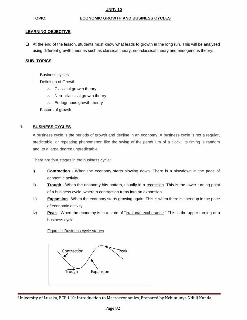
University of Lusaka, ECF 110: Introduction to Macroeconomics, Prepared by Nchimunya Ndiili Kunda Page 82
UNIT: 10
TOPIC: ECONOMIC GROWTH AND BUSINESS CYCLES
LEARNING OBJECTIVE:
At the end of the lesson, students must know what leads to growth in the long run. This will be analyzed
using different growth theories such as classical theory, neo-classical theory and endogenous theory..
SUB- TOPICS:
- Business cycles
- Definition of Growth
o Classical growth theory
o Neo –classical growth theory
o Endogenous growth theory
- Factors of growth
1. BUSINESS CYCLES
A business cycle is the periods of growth and decline in an economy. A business cycle is not a regular,
predictable, or repeating phenomenon like the swing of the pendulum of a clock. Its timing is random
and, to a large degree unpredictable.
There are four stages in the business cycle:
i) Contraction - When the economy starts slowing down. There is a slowdown in the pace of
economic activity.
ii) Trough - When the economy hits bottom, usually in a recession. This is the lower turning point
of a business cycle, where a contraction turns into an expansion
iii) Expansion - When the economy starts growing again. This is when there is speedup in the pace
of economic activity.
iv) Peak - When the economy is in a state of "irrational exuberance." This is the upper turning of a
business cycle.
Figure 1: Business cycle stages
Contraction Peak
Trough Expansion

University of Lusaka, ECF 110: Introduction to Macroeconomics, Prepared by Nchimunya Ndiili Kunda Page 83
2. DEFINITIONS OF GROWTH
Generally economic growth is an increase in the nation's capacity to produce goods and services and
usually refers to real GDP growth. The increases must occur after adjustments for inflation have been
made. There are different growth theories that define economic growth such as classical growth theory,
neo-classical growth theory, endogenous growth theory.
2.1 Classical growth theory
The modern conception of economic growth was began by the Scottish Enlightenment thinkers such as
David Hume and Adam Smith, and the foundation of the discipline of modern political economy. The
theory of the physiocrats was that productive capacity, itself, allowed for growth, and the improving and
increasing capital to allow that capacity was "the wealth of nations". Whereas they stressed the
importance of agriculture and saw urban industry as "sterile", Smith extended the notion that
manufacturing was central to the entire economy.
David Ricardo argued that trade was a benefit to a country, because if one could buy a good more
cheaply from abroad, it meant that there was more profitable work to be done here. This theory of
"comparative advantage" would be the central basis for arguments in favor of free trade as an essential
component of growth.
2.2 Neo – classical growth theory
This model, developed by Robert Solow and Trevor Swan in the 1950s, was the first attempt to model
long-run growth analytically. According to this view, the role of technological change became crucial,
even more important than the accumulation of capital.. This model assumes that countries use their
resources efficiently and that there are diminishing returns to capital and labor increases.
The neo-classical model makes three important predictions:
- First, increasing capital relative to labor creates economic growth, since people can be more
productive given more capital.
- Second, poor countries with less capital per person will grow faster because each investment in
capital will produce a higher return than rich countries with ample capital.
- Third, because of diminishing returns to capital, economies will eventually reach a point at which
no new increase in capital will create economic growth. This point is called a "steady state".
The model also notes that countries can overcome this steady state and continue growing by inventing
new technology. In the long run, output per capita depends on the rate of saving, but the rate of output
growth should be equal for any saving rate. In this model, the process by which countries continue
growing despite the diminishing returns is "exogenous" and represents the creation of new technology
that allows production with fewer resources. Technology improves, the steady state level of capital
increases, and the country invests and grows. The data does not support some of this model's

University of Lusaka, ECF 110: Introduction to Macroeconomics, Prepared by Nchimunya Ndiili Kunda Page 84
predictions, in particular, that all countries grow at the same rate in the long run, or that poorer countries
should grow faster until they reach their steady state. Also, the data suggests the world has slowly
increased its rate of growth.
However modern economic research shows that the baseline version of the neoclassical model of
economic growth is not supported by the evidence. Calculations made by Solow claimed that the
majority of economic growth was due to technological progress rather than inputs of capital and labor.
2.3 Endogenous growth theory
This theory is also known as the new growth theory that was initiated by Paul Romer in the late 1980s
and early 1990s. Other important new growth theorists include Robert E. Lucas and Robert J. Barro.
Unsatisfied with Solow's explanation, economists worked to "endogenize" technology in the 1980s. They
developed the endogenous growth theory that includes a mathematical explanation of technological
advancement This model also incorporated a new concept of human capital, the skills and knowledge
that make workers productive. Unlike physical capital, human capital has increasing rates of return.
Therefore, overall there are constant returns to capital, and economies never reach a steady state.
The new growth theorists concluded that growth does not slow as capital accumulates, but the rate of
growth depends on the types of capital a country invests in. Research done in this area has focused on
what increases human capital (e.g. education) or technological change (e.g. innovation).
Recent empirical analyses suggest that differences in cognitive abilities, related to schooling and other
factors, can largely explain variations in growth rates across countries. Cognitive abilities comprise
intelligence and knowledge and are more important than education itself. Cognitive abilities are more
relevant than the classical growth factor "economic freedom". In comparison of low, mean and high
ability groups within societies the competence level of the high ability group is the most important,
stimulating through research and innovation economic growth and other favorable aspects of countries
like democracy.
3. FACTORS OF GROWTH
One way that output can increase is if there is an expansion in the inputs used to produce it, that is
capital and labor.
There are five kinds of capital. Human-produced capital is called manufactured capital to distinguish it
from the other kinds of capital. Land and natural resources are natural capital, and all the skills and
knowledge possessed by humans are also a kind of capital – human capital. We also note the
importance of social and financial capital, which both refer to institutional arrangements that make
production possible.
University of Lusaka, ECF 110: Introduction to Macroeconomics, Prepared by Nchimunya Ndiili Kunda Page 85
Economists sometimes think about output as being generated according to a "production function,"
which is a mathematical relation between various inputs and the level of output.
Output = f( L, K)
In the most general sense we might say that the output of an economy should be expressed as a
function of flows from all the different types of capital that make production possible. The inputs to the
production function are commonly referred to as factors of production. In the production functions most
commonly used by economists, the factors that are emphasized are manufactured capital and labor.
Sometimes, but not always, natural resources also are included.
3.1 Modeling Economic Growth –Solow Robert
One very influential, and more specific, model of economic growth was developed by economist Robert
Solow in 1957. In his model, he assumed that an economy-wide production function can be written in the
simple form:
Y = A K0.3
L0.7
Where:
Y is aggregate output,
A is a number based on the current state of technology as described below,
K is a quantitative measure of the size of the stock of manufactured capital,
L is the quantity of labor used during the period of time.
K and L are the only factors of production explicitly included in the model. Both capital and labor are
needed for the production of output, with the exponents in the equation reflecting their relative
contributions.
A is called total factor productivity, and includes all contributions to total production not already reflected
in levels of K and L. Often, ―total factor productivity‖ has been interpreted as reflecting the way in which
technological innovation allows capital and labor to be used in more effective and valuable ways. For
example, the development of computer word-processing greatly increased efficiency compared to the
use of typewriters. Typewriters, which seem antique to us today, were themselves a huge productive
advance over clerical work using pen and paper. This process of improved technological methods has
resulted in an increase in labor productivity – more output can now be produced with fewer labor-hours.

University of Lusaka, ECF 110: Introduction to Macroeconomics, Prepared by Nchimunya Ndiili Kunda Page 86
After some mathematical manipulations, the production function above can be converted to an equation
for the growth rate of output per worker as a function of ―total factor productivity‖ and the growth rate of
manufactured capital per worker:
Growth rate of output per worker = growth rate of total factor productivity + 0.3 (growth rate of
manufactured capital per worker)
For example:
if ―total factor productivity‖ grows at 1% per year
and capital per worker grows at 2% per year,
this equation says that output per worker will grow at 1.6% per year
(1% + (0.3)2% = 1.6%).
This became known as the ―growth accounting‖ equation.
Note that output per worker is what is commonly referred to as ―labor productivity‖. While labor
productivity and GDP per capita are not quite equivalent (some people in the population do not work, for
example), they are obviously closely related. Thus, this model implies that the way to raise income per
capita—to achieve economic growth—is to increase the amount of capital that each person works with
(the second term) and improve technology (the first term).
The use of the Solow growth model served to highlight some important factors in economic growth. In
particular, the model led to much discussion of the role of savings in providing the basis for growing
levels of manufactured capital per worker. Technological change also received attention, since this was
thought to be the main driver behind growth in the value of "A." For many years, economists tended to
treat growth as primarily a matter of encouraging savings, investment, and the creation and
dissemination of technology.
In more recent years, other economists have suggested that perhaps this model has directed too much
attention to savings and technology. Some have argued that other factors such as good institutions that
support markets, innovations in the organization of work, or access to global markets should be thought
of as equally important in promoting economic growth. It is not helpful, they suggest, to fold all issues of
social, human, financial and natural capital into just one, rather vague, "A" term
University of Lusaka, ECF 110: Introduction to Macroeconomics, Prepared by Nchimunya Ndiili Kunda Page 87
BIBLIOGRAPHY
Begg.D, Fischer. S & Dornbusch .R (2005), Economics, Mc-Graw –Hill Education, UK
Blanchard. O ( 2009), Macroeconomics, Pearson Education International
Layton Robinson & Tucker, 2009, Economics for Today, Pearson Education Australia
Poole.H (2000), Principles of Economics, D. C Heath and Company, Toronto
Samuelson.N (2007), Economics, Mc –Graw-Hill, New York
Thomas.S.R (2006), Inflation Causes and Cures, Centre for free Enterprise,
Texas A & M University, College Station, TX
Wilson.G.W (1982), Causes and Cures of Inflation, Indiana University
Press, Bloomington