University of New South Wales

School of Economics

Honours Thesis

Hedonic Pricing and the User Cost of Housing in theNetherlands

Author:

Aaryn Lally

Student ID: 3373062

Supervisor:

Assoc. Prof. Glenn Otto

Prof. Kevin Fox

Bachelor of Commerce/Economics (Economics, Econometrics, Finance) (Honours)

28th October, 2016

0.1 Declaration

I hereby declare that this submission is my own work and that, to the best of my

knowledge, it contains no material which has been written by another person or

persons, except where due acknowledgement has been made. This thesis has not

been submitted for the award of any degree or diploma at the University of New

South Wales, or at any other institute of higher education.

Aaryn Lally

28th October, 2016

i

0.2 Acknowledgements

First, I would like to thank my supervisors Professor Kevin Fox and Associate

Professor Glenn Otto for their expertise, guidance, time, and encouragement during

this year. Their passion for real estate economics and empirical measurement, and

years of wisdom in the research field, provided invaluable insight.

I would also like to thank Dr. Iqbal Syed for always being open to have a chat about

my research, and providing useful feedback I could incorporate into my research. A

special thanks also to Professor Jan de Haan for providing access to the Assen data

set and his feedback on the direction of my research findings.

I would like to thank my family for their support and encouragement this year. Last

of all, a special thanks to the 2016 Economics Honours Cohort. I really appreciate

the encouragement and support, and all the honours room banter that made the

year enjoyable.

ii

Contents

0.1 Declaration . . . . . . . . . . . . . . . . . . . . . . . . . . . . . . . . i

0.2 Acknowledgements . . . . . . . . . . . . . . . . . . . . . . . . . . . . ii

Table of Contents iii

0.3 Abstract . . . . . . . . . . . . . . . . . . . . . . . . . . . . . . . . . . 1

1 Introduction 2

2 The Netherland’s Residential Property Market 6

3 Literature 13

3.1 Hedonic Price Methods . . . . . . . . . . . . . . . . . . . . . . . . . . 13

3.2 Stratified Hedonic Indices . . . . . . . . . . . . . . . . . . . . . . . . 18

3.3 User Cost of Housing . . . . . . . . . . . . . . . . . . . . . . . . . . . 19

3.4 Empirical Evidence of Hedonic Pricing . . . . . . . . . . . . . . . . . 22

4 Data 27

4.1 Assen Housing Sector: Variable Description . . . . . . . . . . . . . . 27

4.2 Assen Housing: Data Cleaning . . . . . . . . . . . . . . . . . . . . . . 31

4.3 Assen Housing: Key Data Characteristics . . . . . . . . . . . . . . . . 32

5 Hedonic Pricing Model 36

5.1 Preliminary Hedonic Model Form . . . . . . . . . . . . . . . . . . . . 36

5.2 The Basic Builder’s Model . . . . . . . . . . . . . . . . . . . . . . . . 39

5.2.1 Constant Depreciation Calculation . . . . . . . . . . . . . . . 44

5.3 Creating the Basic Builder’s Model as One Regression . . . . . . . . . 45

6 Hedonic Pricing Under Linear Splining of Land Plot Size 47

6.1 Hedonic Price Analysis: Linear Splining with One Breakpoint . . . . 47

6.2 Hedonic Price Analysis: Linear Splining with Two Breakpoints . . . . 51

6.3 Hedonic Price Analysis: Linear Splining with Nine Breakpoints . . . . 54

7 Hedonic Pricing with Exogenous Construction Cost Data 57

iii

8 Significance of Other Land and Structure Quality Characteristics 62

8.1 Final Builder’s Model . . . . . . . . . . . . . . . . . . . . . . . . . . . 66

9 Investigating the User Cost of Residential Property 69

9.1 Additional Data for User Cost of Housing Calculation . . . . . . . . . 69

9.1.1 Marginal Income Tax Rate . . . . . . . . . . . . . . . . . . . . 69

9.1.2 Risk-Free Interest Rate . . . . . . . . . . . . . . . . . . . . . . 70

9.1.3 Property Tax Rate . . . . . . . . . . . . . . . . . . . . . . . . 70

9.1.4 Maintenance and Depreciation Costs . . . . . . . . . . . . . . 71

9.1.5 Risk Premium of Home Ownership . . . . . . . . . . . . . . . 72

9.1.6 Expected Capital Gains . . . . . . . . . . . . . . . . . . . . . 72

9.2 Applying Poterba’s Framework to Assen Housing . . . . . . . . . . . 73

9.3 Theoretical versus Market User Cost . . . . . . . . . . . . . . . . . . 74

10 Implications for the Real Estate Sector 77

11 Concluding Remarks 80

12 Appendix 81

iv

0.3 Abstract

This thesis provides insight into the contribution of land and structure to property

prices, and investigates housing affordability and market disequilibrium in The

Netherland’s residential property sector. Hedonic regression methods are used

to perform an additive decomposition of property prices into land and structure

components for detached housing in Assen. This analysis indicates structure size,

land plot size, structure age, parking quality and house maintenance quality are

significant factors in determining the land and structure values of a house. Poterba’s

(1984) user cost of capital framework is used to find evidence of disequilibrium in

the housing market, where home ownership has been affordable relative to renting

in Assen over time.

1

Chapter 1

Introduction

Real estate ownership is an important component of household wealth, and housing-

related expenses make up a significant proportion of overall household consumption.

Housing wealth has been observed to have a more significant impact on household

consumption than stock price movements (Case et al, 2005). Capital accumulation

through homeownership has continued to increase, and property taxation makes up

a significant proportion of government funding sources. As a result, strong property

market growth in countries such as the U.S. and Australia combined with stable

prevailing economic conditions have been a driving factor in sustaining high levels

of economic growth.

Following the Global Financial Crisis (GFC), uncertainty has increased in regards

to the market and government understanding how house prices and supply-demand

mechanisms are evolving. It is crucial for the government, households and investors

to enhance their understanding of house price movements to achieve financial

and economic growth and stability. The Reserve Bank of Australia (RBA) has

identified understanding conditions and prospects in the housing sector as a key

policy issue, with a focus on housing affordability, the supply and demand for

housing, and the broader macroeconomic context. This will provide central banks

insight into how real estate impacts economic growth, monetary policy and inflation

measurement, thereby improving economic management and welfare. Additionally,

accurate pricing of real estate and assessment of real estate sector risks is critical

for national statistical agencies such as the Australian Bureau of Statistics (ABS)

to keep accurate national accounts on capital and land stocks over time, and to

measure the Consumer Price Index (CPI). Furthermore, local governments can use

the land and structure decomposition to gain a more accurate measure of property

tax rates on land and structure components.

Typically, national statistical agencies such as the Australian Bureau of Statistics

measure house prices on a periodic basis to track house price changes. This involves

tracking the median sales price for a given region over time and using these prices

to create a house price index. This is based on a matched models methodology,

where the details and prices of a representative selection of houses are collected in

2

a base reference period and their matched prices collected in successive periods.

Measuring house prices in this manner is limited in its ability to capture house

quality adjustments over time and space, and therefore the constructed price indexes

will provide misleading results because the mix of houses sold changes rapidly over

time. This creates matched models sample selection bias, where the sample is

unrepresentative of the residential property sector. This limitation can be overcome

by decomposing property prices into it’s land and structure components separately.

This recognises taxation and depreciation differences between the land and structure

components of a property, and controls for quality changes when measuring price

changes (Francke and Vos, 2004). The decomposition will indicate what fundamental

housing characteristics are driving house price movements and whether market

values for houses reflect the true intrinsic value of real estate over time.

A striking case to analyse is The Netherland’s residential real estate sector. The

Dutch housing boom has been a key factor in enabling The Netherlands to maintain

a stable level of economic growth of 2.19% per annum on average from 1995 to

2015 (CBS Statline, 2016). Following the Global Financial Crisis, the valuation and

quality of Dutch real estate has come under increased scrutiny from government

regulators, households, and the financial sector following recent economic, legislative,

and political changes in the Euro zone. Gaining an understanding of the evolution

of housing supply-demand mechanisms and house prices is important to understand

the level of risk for investors, households and the government in the residential real

estate sector. Understanding the key risk factors in the housing sector will allow the

market and government to understand the potential contagion effects and systematic

risk that The Netherland’s real estate sector poses for the Euro zone and the global

economy.

The Netherland’s government has pursued a range of highly interventionist gov-

ernment policies (both direct and indirect intervention) in the residential property

sector in an attempt to improve home ownership affordability. These policies include

government subsidies, spatial planning laws, zoning regulations, financial guarantees

on mortgages taken out by low-income households, stricter regulation of housing

associations, stricter rent controls, development of financial instruments with higher

loan-to-value ratios, and higher interest deductibility of mortgages. There remains

debate over how these policies have distorted The Netherland’s residential housing

sector, and what contribution these policies have to structural problems in the Dutch

economy. With this backdrop in mind, I analyse house prices and the user cost of

housing in Assen.

3

To analyse house prices, I create a house price index using a highly detailed data

set for Assen detached housing. To analyse user cost of housing, I apply Poterba’s

(1984) user cost of capital framework to identify market disequilibrium by comparing

the theoretical user cost with actual user cost of housing. This will identify the

affordability of home ownership relative to renting over time.

The house prices are decomposed into it’s land and structure components separately

through a hedonic methodology. Land and structure are treated as price-determining

characteristics through a cost of production approach, where the hedonic price

function is determined by market supply and demand forces. The hedonic price

function generates partial derivatives for all periods t = 1, ..., T, which are marginal

prices (also known as shadow prices). These shadow prices are used to perform the

following additive decomposition in Equation 1.1;

V = pLL+ pSS (1.1)

In this framework the property’s value, V, is equivalent to the property’s selling

price. The property’s value equals the addition of land value and structure value.

Land value equals the land plot size, L, multiplied by the price of a unit of land, pL.

Structure value equals the structure floor space area, S, multiplied by the price of a

unit of structure floor space, pS. The hedonic methodology used in this thesis will

build on this basic empirical relationship.

The thesis is structured as follows. Chapter 2 provides a brief introduction to The

Netherland’s residential property market. Chapter 3 will introduce theory behind

additive decomposition of house prices and the motivation behind the builder’s

model used in this thesis. Poterba’s user cost framework, and empirical results

in the literature for user cost analysis and house price index construction will also

be introduced.

Chapter 4 examines key features of the Assen data set and provides a summary of

the land and structure variables after data-cleaning. Chapter 5 introduces the basic

hedonic framework for new and existing houses. In Chapter 6, I use linear splining

of house prices based on land plot size in an attempt to improve model performance.

Chapter 7 introduces exogenous construction cost data in an attempt to address

multicollinearity in the model. Chapter 8 examines the price-determining power of

other land and structure characteristics in the data set. The final, preferred model is

4

also presented in Chapter 8. Chapter 9 examines the affordability of home ownership

in Assen over time and market disequilibrium using Poterba’s user cost framework.

Chapter 10 considers implications of the thesis’ findings, and further research

directions. Chapter 11 provides a summary of the thesis’ main findings.

5

Chapter 2

The Netherland’s Residential Property Market

The Netherlands is a decentralised unitary state consisting of twelve provinces and

418 municipalities. One of these provinces is called Drenthe, located in the north-

east of the Netherlands (as shown in the red box in Figure 2.1). The capital city

of Drenthe is the municipality called Assen, which is the focus of the empirical

investigation in this thesis.

Assen is a small provincial capital city located approximately 133 kilometres from the

Dutch capital city Amsterdam. Assen lies in a flat, featureless plain approximately

ten metres above sea level. Drenthe is considered a remote and low populated

province, and it’s topography is common of cities in The Netherland’s urban fringe.

The Netherland’s has a very unique topography, where 26% of all land lies below sea

level. The high prevalence of low-lying land has encouraged the Dutch government to

enforce a spatial policy that has created dykes, weirs and polders to ensure accessible

and affordable land for housing development.

Another interesting feature of The Netherlands is their population demographics.

The Netherland’s has the highest density out of all Euro zone countries with 488

people per square kilometre. Statistics Netherlands census data indicates that

Assen’s population has grown approximately 0.86% per annum on average from

59,005 in 2001, to 67,061 in 2016 (CBS Statline, 2014). This indicates that Assen

does not have the same population density-pressures relative to the Netherland’s

average. The Netherland’s has a total population of 16 million people, with 40% of

the population living in the Randstand region (which refers to Amsterdam, Utrecht,

the Hague and Rotterdam). This thesis’ results are unlikely to hold accurately in the

Randstand region due to the effect of population-density on local property markets.

Before analysing some preliminary house price results, the last key feature to note

about The Netherlands is the structure and nature of government policy decisions

and enforcement. The Netherland’s national government uses a key planning and

strategic decision framework to manage a variety of complex policy challenges

in spatial planning, land use, housing allowances, social housing, infrastructure

development, and the provision of public services. The strategic framework is high

6

Figure 2.1: Assen’s Location in The NetherlandsSource: SplendidGlobal: Let’s Start from Netherland’s Entry Mode,

https://splendidglobal.wordpress.com/2013/03/25/

lets-start-from-netherlands-entry-mode/, March 2015.

7

Figure 2.2: Drenthe Total Value of House PurchasesSource: CBS Statline, ‘House Price Index by region; existing own homes; 2010 =

100,’ October 2016.

level and empowers provincial and municipal governments to manage their local

residential property sector.

I present here a quick overview of the real estate sector’s performance in Drenthe

between 1998 and 2008. The total value of house purchases in Drenthe grew 60%

from 1998 to 2008 (from 740 to 1185 million Euros), equal to 5.46% per annum

(Figure 2.2). Over the same time period, the house price index grew 110% from

1998 to 2008 (from 1 to 2.1), or 10% per annum (Figure 2.3). This indicates very

strong and consistent growth in both the prices and value of housing transactions

in Drenthe’s residential housing sector from 1998 to 2008.

The Netherland’s residential property sector has seen heavy use of interventionist

policies to achieve the government’s policy objectives. During the early twentieth

century, The Netherland’s national government focused on providing a greater

quantity of affordable housing, and also focused on how to improve accessibility

to this housing for a greater proportion of the population. To meet these objectives,

the Housing Act was introduced in 1901. The introduction of this legislature greatly

improved median housing conditions in The Netherlands. During this time, the

government enforced zoning areas (allocated by provincial government authorities),

developed new subsidy instruments to provide greater mortgage relief to low-income

household owners, and enforced legislation that required municipal governments to

8

Figure 2.3: Drenthe House Price IndexSource: CBS Statline, ‘House Price Index by region; existing own homes; 2010 =

100,’ October 2016.

provide basic amenities and services for all residential households.

During World War 2, The Netherland’s experienced another huge housing shortage.

This required further intervention by the Netherland’s national government to

provide additional policy instruments to complement the Housing Act. The

Netherland’s government introduced new subsidies for companies that provided

social housing, and set the level of residential gross house rents well below the

market equilibrium level. These policies were hugely effective in enabling a greater

proportion of low income households to enter and remain in the residential property

market as home owners. The policy has had a lasting impact on The Netherland’s

housing market, where The Netherlands has the largest social housing proportion

in the Euro zone at 33% of all dwellings (Vandevyvere and Zenthofer, 2012).

Since the early 1980s, The Netherland’s government has shifted its policy focus

towards improving the median quality of houses. This policy shift has coincided with

an increase in home ownership in The Netherlands from 42% of total dwellings in

1980 to 60% of total dwellings in 2012. To achieve this new policy objective, a range

of government policy and financial market changes have taken place. These include

favourable tax policy for home owners, lower inflation levels, lower real interest rates,

better mortgage-financing instruments, and low supply elasticity for new dwellings.

This policy shift has made the housing sector more market-oriented by decentralising

housing policy to municipalities, gradually removing subsidies for social rental

9

housing, better targeting of housing allowances towards low income households,

and making mortgage payments fully deductible for home owners (Priemus and

Dieleman, 1997).

Although these policy changes have allowed strong sustainable growth in the

residential property sector, this has come at a potential cost to financial stability.

The combination of these changes have relaxed borrowing conditions for home-

owners. In particular, the ability of home-owners to fully deduct interest payments

on mortgage loans from their taxable income up to 30 years, and the opportunity to

invest in newly-introduced investment mortgages (which take advantage of unlimited

mortgage interest payment deductions) have significantly benefitted high-income

earners and incentivised households to borrow more money to acquire property.

Furthermore, credit limitations on banks have been relaxed. Banks can now take

the primary and non-primary income of a household into acccount when determining

the maximum mortgage amounts that can be lent. These policies have significantly

increased the gross debt level in The Netherlands, with this increase strongly driven

by a rise in gross mortgage debt. Currently, The Netherland’s has the highest gross

household debt level as a percentage of GDP in Europe at 111.4%. This worrying

household debt level trend has been persistent in The Netherland’s financial sector

since the Second World War.

A major component of the government’s housing market policy is the National

Mortgage Guarantee System (NMG). As of 2012, the NMG guaranteed $141 billion

Euros worth of mortgage loans (which represents 24% of The Netherland’s total

GDP). The NMG subsidises and stimulates higher home ownership and protects

banks from credit risk (Vandevyvere and Zenthofer, 2012).

To provide a snapshot, the Dutch economy experienced consistently high economic

growth leading up to the late twentieth century, with the Dutch housing boom

a key factor in this trend. Following the recent Global Financial Crisis (GFC),

uncertainty has increased in The Netherland’s residential housing sector. This has

created a decline in transaction volumes and house prices, reflecting increased risk

for consumers and investors of Dutch real estate. Empirically, the mean Dutch house

price fell below the long-run-average for the first time in two decades following the

GFC, decreasing at an average of 3% per annum since 2008. It is likely house prices

in Drenthe also fell following the GFC but this time period is not reported in this

thesis’ analysis. Potential reasons for the observed house price decline following the

GFC are a fall in average household disposable income, tighter lending standards

imposed on banks, lower employment growth, and decreased market confidence in

10

the real estate sector. There are currently significant questions being raised about

the affordability of home ownership and renting in the residential housing market,

and how to make government policy more effective.

It is worth noting The Netherland’s social housing sector as it is a unique feature

of The Netherland’s residential property sector. The Netherland’s has the third

largest stock of social housing in Europe, after France and the United Kingdom.

As of 2005, 2.4 million out of 6.8 million (approximately one third of all dwellings)

in The Netherlands were social rented dwellings and this number has remained

relatively constant up to the present day. Social housing is more prevalent in urban

areas. In particular, 55% of all dwellings in Rotterdam and Amsterdam are social

rented properties.

The proportion of social housing is also reasonably high in remote, less populated

areas like Drenthe which has a social rented housing proportion of 25% of all

dwellings. The majority of this social housing stock was built between 1945

to 1990, where The Netherland’s government was effectively able to incentivise

increased social housing supply in the aftermath of World War 2. Housing

associations supplying social housing were exempted from paying corporate tax,

received subsidised prices for council land, and had their loans guaranteed under

the Guarantee Fund for Social Housing. In response to house price increases over

the last twenty years, the government has abolished these supply-side subsidies and

shifted it’s policy focus to improving housing affordability for first-home buyers.

With this backdrop in this mind, this thesis investigates the following questions.

First, how has the value of Dutch residential real estate changed over time,

accounting for land and structure components separately. This will build on analysis

conducted by Diewert et al (2015) on Assen house sales price data. This thesis

focuses on levels value analysis of the contribution of land value as a percentage of

house value (also called land leverage) over time. The second question addressed

by this thesis is how the affordability of residential property ownership relative to

renting has evolved over time, and whether any patterns exist in observed market

disequilibrium.

The Netherland’s seems a good choice to analyse due to the unique nature of it’s

housing market structure and the high prevalence of government intervention in

the sector. This thesis’ analysis adds to numerous literature studies on user cost

of housing, including in the US (Himmelberg, Mayer and Sinai, 2005; Baker, 2002;

McCarthy and Peach, 2004), Australia (Hatzvi and Otto, 2008), the UK (Weeken,

11

2004), Ireland (Browne, Conefrey and Kennedy, 2013), and Finland (Kivisto, 2012).

To the best of my knowledge, this thesis is the first empirical investigation of housing

user cost in The Netherlands.

12

Chapter 3

Literature

3.1 Hedonic Price Methods

Hedonic regression is a revealed preference method used to estimate the contributory

value of each explanatory characteristic to an item’s price. The contributory

values of each variable is determined by regressing the item’s price on the vector

of characteristics. These methods have many applications in the literature with

particular use in industries experiencing rapid technological change (Diewert, Heravi

and Silver, 2007).

Applied to a housing context, the hedonic model treats real estate as a bundle

of goods sold on the market. The expected transaction price for a house is the

summation of the value of the houses’ characteristics (where the characteristics are

divided into physical and locational factors);

House sales price = f(Physical and Locational factors).

Physical factors measure dwelling quality and include land plot size, structure

floor space, the number of bathrooms, the number of bedrooms, and parking

space available. Locational factors measure the quality of the building site

and include distance to the nearest train station, the provision of shops and

workplaces, neighbourhood characteristics, distance to the capital city, distance to

basic amenities and services such as shopping centres, and environmental quality

(such as noise pollution).

There are limitations on the extent and accuracy to which these factors can

be measured and quantified since there is no market for these characteristics.

Each characteristic can not be sold separately, and therefore the price of each

characteristic is not independently observable. Traditional discount cash flow models

are inapplicable as a result. This thesis uses an additive decomposition framework

to overcome these data limitations.

There are three methodologies that can be used to perform an additive decom-

position of house prices into it’s land and structure values separately. These are the

13

construction cost method, hedonic regression methods, and the vacant land method.

The vacant land method determines the price of a unit of land associated with

a sold property, pL, from the sales of vacant land plots comparable in size and

location. Using the estimated price pL and the house price model V = pLL + pSS,

the price of a unit of housing structure, pS, can be determined. Available land sales

are not likely to be comparable with the date at which they were sold, and there

tends to be a relatively sparse volume of vacant land sales in urban centres (Clapp,

1980). This results in significant accuracy issues with this approach.

The construction cost method uses construction cost per unit of structure area

(measured by National Statistical agencies) as an estimate of the price of a unit of

housing structure, pS. Using this price and the house price model V = pLL + pSS,

the price of a unit of land, pL, can be determined (Glaeser and Gyourko, 2003;

Davis and Palumbo, 2008). There are significant accuracy measures in estimating

unit structure price in this manner, depending on the approach used by a given

statistical agency.

To avoid these accuracy issues, I use a hedonic regression which treats land and

structure as separate characteristics to create a quality-adjusted price index (Diewert

et al, 2015). The hedonic model is estimated using an additive decomposition

framework. The hedonic function generates marginal prices for land and structure

(also called shadow prices) for a given time period as partial derivatives. The

partial derivatives are used to decompose the house price into it’s separate land

and structure components and can be interpreted as the marginal cost of producing

the different characteristics.

This paper only considers physical factors to quality adjust land and structure due

to data limitations with the Assen detached housing dataset. There may be an

omitted variable problem caused by a lack of location data. This can be removed by

explicitly accounting for spatial dependence. Hill et al (2008) suggest incorporating

geospatial data with splines to perform parametric and non-parametric analysis to

allow for spatial dependence. Given suitable data, such an approach would be a

useful extension to this paper’s findings.

The hedonic regression methodology has distinct advantages and disadvantages

over other methods. Advantages of using hedonic regression methods to construct

property price indexes (RPPIs) are;

14

1. Hedonic methods can create separate indexes for land and buildings, which are

very difficult to compile otherwise,

2. Hedonic methods can adjust for sample mix changes and quality changes of

individual properties,

3. Hedonic methods are flexible in constructing price indexes for different types of

property that vary by dwelling-type or location,

4. The matched model approach often used in the literature to value houses is

equivalent to the hedonic imputation method, allowing easy comparison of hedonic

prices with existing literature.

Some of the major disadvantages of using hedonic regression methods to construct

RPPIs are;

1. Hedonic methods are data intensive, and require detailed property characteristics

data for all house sales. Non-homogenous data with respect to location and house

type is ideal for reliable estimation where the sample can be broken into subgroups

that have similar characteristics,

2. There is a high risk of multicollinearity between the land and structure

components which will result in unreliable price estimates,

3. It can be difficult to sufficiently control for location if property prices differ

significantly by region. A common method used to solve this problem is to stratify

hedonic regressions,

4. Hedonic methods require a variety of decisions on functional form, model

transformations, and error term specification. This can make replicating and

validating results difficult with wide variation in price estimates.

5. Measuring quality change of land and structure is difficult. To make this easier, I

assume quality is closely related to the period in which the dwellings are constructed

(since regulation and construction costs change between time periods),

6. The structure values calculated will need to be adjusted to be compared with

capital measurement under the perpetual inventory method.

This paper uses a cost-oriented hedonic model called the builder’s model (Diewert et

al, 2015). For a given time period t, location and type of land, the hedonic regression

model in it’s most simplistic form is Equation 3.1;

V = βS + αL+ ε (3.1)

The builder’s model (both it’s linear and non-linear specifications) are estimated

15

using maximum likelihood estimation on the Assen data. There are two functional

forms commonly used in the literature to create hedonic house price models. The

first approach is the fully linear model (Equation 3.2);

V tn = αtLtn + βtStn + εtn (3.2)

∀t = 1, ..., T ;

∀n = 1, ....., N(t),

The second approach is the semi-log model (Equation 3.3);

lnV tn = αtLtn + βtStn + εtn (3.3)

∀t = 1, ..., T ;

∀n = 1, ....., N(t),

The log-linear model is not valid in an additive decomposition framework, since

house value is simply the addition of land value and structure value. Thus, I use

the linear model for my analysis. In situations where the additive decomposition

framework is not considered, the semi-log specification is advantageous as it can

help reduce heteroskedasticity and allow for constant variance of errors (Diewert,

2003).

For the builder’s model, each property has a sales price, V tn , structure floor space

area, Stn, building cost per square metre, β, land plot area, Ltn, land cost per square

meter, α, and an error term εtn for a given period t, and for n = 1, ..., N(t). The

property price is equivalent to the property’s market value.

I make the stochastic assumption that all houses in the sample are of the same

general type. I assume the error terms εtn are independently and normally distributed

with a mean of zero and constant variance. This is an additive error specification,

and is preferred over the assumption of multiplicative errors in the additive

decomposition framework (Diewert et al, 2015). A potential implication of assuming

16

an additive error specification is that heteroskedastic errors may arise if expensive

properties tend to have relatively large absolute errors relative to cheaper properties

(Koev and Santos Silva, 2008).

In terms of running the hedonic regression, there are two techniques that can be

used to quality-adjusted prices; the hedonic imputation method and the hedonic

time dummy method. Both methods use hedonic regressions to remove the effects

of quality changes on house prices, and can be used in a weighted or unweighted

regression. However, each method yields a different result due to a difference in

the averaging principle used (Pakes, 2003). The hedonic time dummy method

constrains the hedonic regression parameters to be constant over time, whilst the

hedonic imputation index allows the hedonic regression parameters to vary over

time. This makes the hedonic imputation method more flexible in allowing for

quality adjustment changes in each period, and is the preferred method for this

paper.

The hedonic time dummy method provides a useful measure of house price inflation

but does not specify the portion of land and structure value captured by this

inflation term. This makes it very hard to create an accurate land and structure

decomposition of house prices using the hedonic time dummy method.

Multicollinearity is a common problem in hedonic regression methods due to high

correlation between some of the included explanatory variables. There is likely to

be high collinearity between housing characteristics due to the fixed proportions

of these variables in housing construction (for example, between the number of

rooms and structure floor space area). Atkinson and Crocker (1987) use Bayesian

techniques to treat this collinearity and note an important bias-variance tradeoff.

The collinearity results in high standard errors for the regression coefficients, causing

the coefficients to become unstable and increasing mis-measurement bias. The

presence of collinearity raises concerns about specification issues and makes it hard

to predict how different variables affect house prices.

Another common problem in a housing context is omitted variable bias. As noted

by Case et al (1991), it is hard to accurately measure all housing characteristics that

affect house quality and house prices over time. This problem makes it difficult to

predict the magnitude and sign of the bias caused by the omitted variables, resulting

in bias in the constructed hedonic indexes.

17

3.2 Stratified Hedonic Indices

Stratification can be used to adjust for changes in the quality mix of houses sold over

time. My paper heavily draws on these stratification strategies as it seems sensible

that house value may have a non-linear relationship with land plot size. Stratification

techniques were popularised in the analysis of profit rates in the aerospace industry

by Poirier and Garber (1974) who used spline functions to analyse and compare

three distinct time periods. Another example is by Diewert and Wales (1992), who

use adaptive splining to choose a suitable breakpoint specification that allows for

non-linear responses with respect to time in a normalised quadratic profit function.

The number of break points is first set to two, and a grid search is conducted on all

possible combinations of potential break points (where the model with the largest

log likelihood value is selected).

Stratifying the sample creates a piecewise linear function. The function is made up

of a number of linear splines that adjust for changes in the quality mix of properties

sold. An important consideration is choosing a suitable number and position of

splines (Friedman and Silverman, 1989). I use median and percentile measures to

optimise the breakpoint specification.

Using stratification to adjust for quality changes in houses seems sensible, since

it is unlikely a single hedonic model can accurately measure housing dynamics in all

house market segments. Furthermore, stratification helps to reduce sample selection

bias in stock-based RPPIs to produce a more accurate comparison of price trends

between different types of houses and regions.

The alternatives to spline modelling are to use dummy variables or polynomials.

The dummy variable approach fits dummies to blocks of observations to avoid over-

fitting issues. This method provides poor estimation if the model is continuous with

respect to land plot sizes.

The use of polynomials is also undesirable due to constraint considerations with

global fit of the model. De Boor (1979) finds that spline functions are continuously

differentiable to the order of n - 1, whereas polynomials are only continuously

differentiable to the order of n. This makes spline functions more flexible as they can

respond to locally sharp areas of the function without affecting the model’s global fit.

In regards to spline functional form, it is appropriate to use linear splines over

higher order functions since there is no a priori reason to model land plot size in a

18

continuously differentiable manner (Fox, 2012).

In this paper, I stratify house prices by land plot size. This uses a linear land

plot trend to capture potential discontinuities and instantaneous jumps in the house

price function at the spline break points. This will assign a different land price to

properties based on the land plot size. The regression creates a set of variables used

to construct a piecewise linear model. The linear spline function is initially flat and

drops at the breakpoint (capturing a threshold effect) before becoming flat again.

The threshold effect is captured by the two breakpoints which specify the start and

end points of the land pot size slope change.

I assume the regression model is linear between any two corresponding break points

and that the regression is connected at these break points. I also assume that the

quality mix of housing within each constructed spline is the same. The effectiveness

of splining depends on how significantly land prices change as land plot size increases,

and on the amount of unit value bias inherent in the spline model (since each

property sale is a unique good).

3.3 User Cost of Housing

Analysing user cost of housing measures deviations in the market value of houses

from their theoretical equilibrium values over time. Tracking market disequilibrium

changes over time measures the affordability of home ownership relative to renting,

and whether there is evidence of a potential housing market bubble. Conventional

metrics such as price-rent and expenditure-income ratios capture the annual rent

paid for housing consumption and are typically used to measure housing affordability

(Haffner and Boumeester, 2010). These approaches are directly linked to a

household’s relative income and are restricted in analysing how the proportion of

household income spent on housing changes over time (Hulchanski, 1995). The user

cost of housing approach to measuring market disequlibrium and housing bubbles

has become increasingly popular in the real estate literature, such as Syed and Hill’s

(2012) investigation of Sydney property overvaluation.

The user cost of housing at the start of period t is the present value of buying

one unit of housing, using it for period t, and than selling this unit of housing

(Diewert, 1974; Hicks, 1939). This equals the rate of return on housing over period

t, which is equivalent to the cost of renting a house for period t. This approach to

measuring cost is useful because it factors in asset-class risk as well as idiosyncratic

19

risk for homeowners.

Poterba’s user cost of capital framework (Poterba, 1984) is a neoclassical investment

model used to study housing demand and analyse the equilibrium imputed rental

income for homeowners. An owner-occupier of real estate forgoes interest on the

dwelling’ s market value, incurs property taxes, incurs depreciation and maintenance

costs, incurs risk from uncertainty of future house prices and gross rent movements,

and benefits from the dwelling’s future capital gains. The user cost of housing is

calculated using Equation 3.4;

UCt = rt + αt + δ + γ − βt (3.4)

where;

− UCt is the per dollar cost of owning one unit of housing for period t (where t

is measured in years),

− rt is the risk-free interest rate for period t,

− αt is the local property tax rate for period t,

− δ is the maintenance and depreciation rate for period t,

− γ is the required risk premium to invest in one unit of housing relative to

renting, and

− βt is the expected house price appreciation from year t to year t+1.

∀t = 1, ..., 11

At equilibrium, the theoretical equilibrium cost of renting equals the price-rent ratio

(Shiller, 2006) as shown in Equation 3.5;

UCt =Rt

Pt(3.5)

where;

− UCt is the per dollar user cost of capital for period t,

20

− Rt is a given household’s imputed rental income per unit of housing capita for

period t,

− Pt is the asset price of a unit of housing capital for period t, and

− UCt ∗ Pt is the user cost of capital for period t.

∀t = 1, ..., 11

To evaluate the equilibrium empirically, the expression is often re-expressed as

Equation 3.6;

PtRt

=1

UCt(3.6)

The price-rent ratio in the market should equal the inverse of the per dollar user

cost. If the actual market rent is higher than the theoretical user cost (Rt > UCtPt),

than it is cheaper for households to buy housing relative to renting. Since owner-

occupying is more attractive than renting, this puts upward pressure on house prices

and downward pressure on gross rent until equilibrium is restored. If the theoretical

user cost is higher than actual market rent, the opposite argument applies. Renting

will be cheaper relative to buying and this decreases pressure on house prices and

increases pressure on gross rent until market equilibrium is achieved.

The equilibrium framework assumes that the price-rent ratio is the same for all

types of owner-occupiers and assumes Pt and Rt are calculated for properties of

equal quality. This is unlikely to hold in practice where Pt and Rt vary across

age and income groups. There is a quality mismatch between median houses in

the rental and owner-occupier housing markets. Furthermore, the variables used

to calculate user cost aren’t directly observable and approximation of these inputs

creates mis-measurement bias (Verbrugge, 2008).

21

3.4 Empirical Evidence of Hedonic Pricing

The conceptual motivation for performing hedonic methods was first explained by

Lancaster (1966) and Rosen (1974). Lancaster and Rosen broke away from the

traditional approach of treating goods as direct objects and utility, and instead

assumed utility is derived from the goods’ characteristics and properties. In

recent years, quality-adjustment of house prices has become a major focus to gain

greater understanding of house price dynamics. There are two main approaches to

conducting house price hedonic analysis; the hedonic imputation method and the

hedonic time dummy method.

Before investigating the user of hedonic methods, I consider other methods in the

literature to analyse house prices. First, transactions data on a microeconomic level

can be used to quality-adjust house prices. One such application of this methodology

is by Wu, Deng, and Liu (2014) who create a constant-quality house price index using

transactions data for new housing units in China. The data set is obtained from the

Real Estate Market Information System (REMIS) for thirty-five Chinese cities, and

provides detailed characteristics and information on all new housing unit sales from

2006 onwards across China. They observe a dramatic price surge across China from

2006 to 2010. The framework provides a good method that can be employed in The

Netherland’s on how to collect data to construct accurate city hedonic price indexes.

Another approach to modelling house prices is a simultaneous equations framework.

Chow and Niu (2013) utilise a simultaneous equations framework to analyse supply

and demand for Chinese urban residential housing. Demand is equal to Equation

3.7;

qt = b0 + b1yt + b2pt + u1t (3.7)

Supply is equal to Equation 3.8;

qt = c0 + c1pt + c2ct + u2t (3.8)

In this framework, qt is housing space per capita, yt is real disposable income per

capita, pt is the relative price of housing, and ct is the real construction cost. Using

reduced form equations, Chow and Niu (2013) find that rapid housing price growth

is well explained where income determines demand and construction costs affect

supply.

Finally, Gyourko (2013) uses spatial data on US residential property to analyse the

22

government’s regulation of residential property. Gyourko finds empirical evidence

that local zoning policies and land-use restrictions influence housing supply elasticity

in a statistically and economically significant way. This has important implications

for analysing the impact of highly intervenionist government policies on The

Netherlands’ property sector.

The above methods are not applicable to this thesis’ investigation as they do

not allow an accurate deconstruction of house prices into it’s land and structure

components. Hedonic regression methods provide a useful method for such analysis.

Gyourko et al (2015) create a constant-quality hedonic price index to construct

price-rent and price-income ratios for China’s three property tiers. This framework

utilises a microeconomic data set that measures housing supply, housing demand,

rent data, depreciation data, and real land prices. Using the constructed ratios,

Gyourko et al (2015) find evidence of high user cost of housing in China’s larger cities.

This is potential evidence for poor housing affordability and strong over-valuation of

property in these areas. The finding is empirically justified by considering expected

future capital gains for real estate in China’s larger cities.

Syed et al (2008) construct quarterly temporal and spatial hedonic price indexes for

Sydney housing. The paper uses temporal fixity (Hill, 2004) to manipulate shadow

prices so they are flexible across regions and time. This breaks the regression up into

overlapping blocks that are spliced together. This overcomes spatial dependence

in the shadow prices by spatially weighting the neighbourhood of observations.

This creates more efficient estimators and corrects standard errors. House prices

are than estimated using maximum likelihood estimation (Anselin, 1988). This

helps overcome spatial dependence by spatially weighting the neighbourhoods of

observations, which creates more efficient estimators and corrects standard errors.

Furthermore, the paper uses multiple imputation techniques to solve missing data

issues and to correct for heteroskedasticity (Rubin, 1987). The significance in the

literature placed on accounting for spatial dependence has increased due to the

influence of spatial correlation on hedonic results where house prices are obtained for

neighbourhoods that share locational amenities or consist of dwellings with similar

structural characteristics (Basu and Thibodeau, 1998). The method is not applied to

Assen due to data limitations but would be a useful extension to my paper’s analysis.

An early use of hedonic methods to create an additive decomposition model is

by Bostic et al (2007) who use an additive decomposition model to demonstrate

how land leverage explains the majority of variation in house price appreciation in

23

Kansas. Land leverage is equal to land value as a proportion of house value. The

paper employs a framework similar to Davis and Heathcote’s (2007) analysis of the

U.S. market from 1975 to 2000. Land leverage is investigated by comparing the price

of vacant land plots with prices of the same properties after houses are constructed

on the vacant land plot. An alternative measure of land leverage is to use assessed

values for land provided by local property tax assessment offices. This focus on land

leverage has become popular in the literature with a variety of applications. An

example is Bourassa et al’s (2009) measurement of land leverage in New Zealand.

Bourassa et al (2009) find that houses with a higher land leverage value are more

price-volatile over the entire property cycle.

Building on Bostic et al’s (2007) approach, Diewert et al (2015) use the hedonic

imputation method to create a land and structure decomposition model called the

builder’s model (Equation 3.9);

V tn = αtLtn + β1pt(1− δtAtn)(1 + γRt

n)Stn + εtn (3.9)

Diewert et al (2015) consider linear splining and adding exogenous information to

the model to find the builder’s model explains 87% of house price variation in Assen

from 1998 to 2003. The paper provides the motivation for the methods employed

in this thesis. This thesis considers the land and structure values in Assen from

1998 to 2008 on a levels basis, which allows comparison with the index land and

structure prices calculated by Diewert et al (2015). Furthermore, this thesis analyses

the relative affordability of home ownership versus renting over time in Assen. The

implications of house prices on housing affordability are not considered by Diewert

et al (2015).

A common issue in hedonic regression analysis is how to treat missing data

appropriately to avoid mis-measurement and bias. Syed et al (2008) provide a

framework that uses multiple imputation techniques developed by Rubin (1987) to

solve missing data issues, and use this to correct for heteroskedasticity. The paper

demonstrates how to perform hedonic regressions to provide detailed analysis of the

impact of interaction terms between housing characteristics, different regions and

different time periods on house prices. These methods provide motivation on the

modelling strategy used in this thesis and help improve model flexibility and remove

substitution bias.

Another strategy that can be used to improve hedonic regression decomposition

models is to use a dynamic identification strategy. Rambaldi et al (2015) create a

24

land and structure decomposition (using a dynamic identification structure through

a Kalman filter) to find land value is significantly larger proportion of house value

than structure value in Brisbane and the San Francisco Bay Area. Application of the

Kalman filter to the Assen data set may help improve the identification strategy for

separating land and structure values separately but is not considered in this paper

due to a lack of detailed location data.

The literature on residential house price movements in The Netherlands focus on

using price indexes created by Statistcs Netherlands (CBS Statline). There are a

variety of such studies including Kakes and Van Den End (2004) who investigate the

link between stock prices and house prices, Shiller (2007) who investigates trends

between house prices and home ownership, and Boelhouwer (2005) who investigates

the effect of incomplete privatisation in The Netherlands on house price dynamics.

The house price data used in these investigations in not valid for comparison with

results in this thesis as they are not applicable in an additive decomposition context.

Using these house prices, the relative change in the affordability of owning a house

can be conducted using Poterba’s (1984) framework, where the marginal cost of

housing services equals the marginal benefit of housing services. Poterba analyses

the user cost of housing service per unit of housing, and compares this with the rate

of gross housing market rent which is interpretable as the marginal benefit. In other

words, individuals will consumer housing services until the marginal value of using

housing services equals the marginal cost of the housing service. The user cost per

unit of housing service is equal to Equation 3.10;

w = [δ +K + (1− θ)(i+ µ)− πH ] (3.10)

The framework assumes all housing units depreciate at a constant rate δ and require

maintenance equal to K times the total current house value. Furthermore, property

tax liabilities at a rate of µ are imposed on owner-occupiers, who can deduct property

taxes from their taxable income where a given individual faces the marginal income

tax rate θ. Finally, owner-occupiers expect capital gains of πH over the coming year

on their house and can borrow or lend at the nominal interest rate i. Using this user

cost approach provides the motivation for the measurement of housing affordability

in this thesis.

Himmelberg et al (2005) use Poterba’s (1984) user cost framework to measure the

user cost of housing for single-family households in U.S. metropolitan areas. They

find conventional measures of housing affordability in the literature such as price-

25

rent ratios, house price growth rates and price-income ratios yield misleading results.

These conventional measures of the affordability of housing are unable to indicate

whether house price increases are increasing ownership costs because the price of

a house is not equivalent to the annual cost of owning that house. Furthermore,

calculation of the ratios is heavily dependent on assumptions of expected house

price appreciation and future tax rates. This can cause significant variation in

calculated price-rent ratios. Finally, house prices are more sensitive to interest rate

changes when real interest rates are low or in cities where the long-run growth rate

of house prices is high. In these situations, observed price growth may inaccurately

provide evidence of a house price bubble. Himmelberg et al (2005) overcome these

inaccuracies by imputing the annual rental cost of owning a home and evaluate this

as the cost of owning a house. Using Poterba’s user cost framework, Himmelberg

et al (2005) find evidence of overvaluation in the owner-occupier housing market

during the 1980s, and that these house prices have corrected towards the long-term

trends. This indicates that overvalued houses have experienced large price decreases

to correct towards market equilibrium over time. Furthermore, Himmelberg et al

(2005) find that the cost of owning a house relative to renting increased in most U.S.

cities from 1995 to 2004. This evidence suggests housing affordability in the rental

market has improved over time.

Syed and Hill (2012) build on Syed et al’s (2008) investigation by using quality

adjusted price-rent ratios and observed price-rent ratios in the property market

to analyse the user cost of housing in Sydney. The paper finds evidence of

disequilibrium in the Sydney property market, where home ownership is overvalued.

The paper notes key issues that must be considered when working with the user

cost framework. Since median owner-occupied housing are of a higher quality

than median rented dwellings on average (Hatzvi and Otto, 2008), bias may arise

due to quality mismatches. To avoid this, price-rent ratios should be matched

at the individual dwelling level. This data is not available because dwellings are

sold and rented at different times. Syed and Hill (2012) use hedonic methods to

estimate price-rent ratios at the individual dwelling level and assume price-rent

ratios computed under the user cost framework measure the same dwelling as market

price-rent ratios. Another key issue is the sensitivity of price-rent ratios to expected

real capital gains on housing (Verbrugge, 2008). Syed and Hill impute expected

capital gain implied by the user cost framework to measure forecasted expected

capital gains.

26

Chapter 4

Data

4.1 Assen Housing Sector: Variable Description

My thesis uses a panel data set consisting of 6,397 sales records of detached houses

in Assen from the first quarter of 1998 to the second quarter of 2008. Note that

further data sources are used for user cost housing measurement. These sources are

presented in a later section of this thesis. For each house sale in Assen, the data

set contains corresponding quantitative and qualitative information for key physical

and locational attributes. There are no missing observations or non-response issues

with the initial data set (which are typically common in empirical hedonic regression

studies). The information is a mixture of continuous and dummy variables.

Table 4.1: Variable Definitions

Value Description Measurement Units

V tn Sales price for property n sold in quarter t 1000s of EurosLtn Land plot size for property n sold in quarter t m2

Stn Floor space area for property n sold in quarter t m2

BP tn Decade in which property n sold in quarter t is built 0 to 9

Atn Decade age of property n sold in quarter t 0 to 4Rtn Number of rooms for property n sold in quarter t Units

T tn Number of toilets for property n sold in quarter t UnitsF tn Number of floors for property n sold in quarter t UnitsBLtn Number of balconies for property n sold in quarter t UnitsDtn Number of dormers for property n sold in quarter t Units

RT tn Number of roof terraces for property n sold in quarter t UnitsBT tn Number of bathrooms for property n sold in quarter t UnitsP tn Parking quality for property n sold in quarter t 0 to 5MI tn Inside house maintenance of property n sold in quarter t 0 to 9MOt

n Outside house maintenance of property n sold in quarter t 0 to 9SH t

n Garden storage quality for property n sold in quarter t 0 to 6LRt

n Living room area for property n sold in quarter t UnknownCtn Construction costs for property n sold in quarter t Index (1998 = 1)

Qtn Quarter in which property n is sold Units

A description of the housing characteristics used in my analysis is provided in Table

4.1 ∀ t = 1, ..., 42 and ∀ n = 1, ...., 6397. This thesis analyses linear prices, since

27

the semi-log model specification is not interpretable or valid under the additive

decomposition framework.

The quarter variable is constructed from observed contract registration date.

Structure size is measured using the structure’s floor space area Stn. The mean

structure floor space area is 125.72m2, with the smallest house having a floor space

area of 55m2 and the largest house having a floor space area of 352m2. The median

and modal floor space area for detached housing in Assen is 120m2.

The number of floors variable F tn is not used in my analysis due to uncertainty

over whether the building floor data is measuring apartment numbers rather than

number of floors.

The structure age variable Atn is constructed using building period data and is

defined in Equation 4.1;

Structure age = 9−Building period (4.1)

The interpretation of the decade structure age is provided in Table 4.2. For example,

a house built between 1960 to 1970 is assigned a value of 4 and so on. The variable

measures the increase in structure price per square metre when moving from one

decade structure age to the next. The median structure age is 2 (1981 to 1990) with

an average of 1.99 (1981 to 1990). The largest number of houses are built from 1991

to 2000.

Table 4.2: Structure Age Description

Decade Structure Age Value

2001 - 2008 01991 - 2000 11981 - 1990 21971 - 1980 31961 - 1970 4

∀t = 1, ..., 42;

∀n = 1, ...., 6397.

28

The interpretation of parking quality is provided in Table 4.3. For example, a house

that has a garage and one carport will be assigned a value of 4. In general, the

higher the parking quality value, the higher the structure price per square metre.

Table 4.3: Parking Availability Description

Parking Quality Value

No parking 0Parking space 1Carport with no garage 2Garage with no carport 3Garage and carport 4Garage for multiple vehicles 5

The inside maintenance variable measures the quality of maintenance performed

inside a house, on a scale from bad to excellent. I assume this variable captures

maintenance performed to the inside and outside of the houses’ structure component,

but excludes any maintenance performed to the physical land plot that the structure

sits on. The scale of values for inside maintenance is shown in Table 4.4. For

example, a house with reasonable to good inside maintenance is assigned a value of

6. As inside maintenance increases, this reflects a greater quality of housing structure

resulting in an increase in structure price per square metre. Note that this variable

does not indicate the cost or amount of maintenance performed to the inside of the

structure. To enable more accurate analysis of the impact of renovation quality on

structure value, data measuring the dollar value maintenance improvements to a

house would be ideal to capture these effects.

Table 4.4: Inside Maintenance Description

Inside Maintenance Quality Value

Bad 1Bad to moderate 2Moderate 3Moderate to reasonable 4Reasonable 5Reasonable to good 6Good 7Good to excellent 8Excellent 9

29

The outside maintenance variable measures the quality of maintenance performed

to the physical land plot that the structure sits on. The variable is measured on

a scale from bad to excellent as shown in Table 4.5. For example, a house with

good outside maintenance is assigned a value of 7. As outside maintenance quality

increases, this reflects a greater quality of land plot resulting in an increase in land

price per square metre. Again, more detailed analysis will be possible if data is

available on the dollar value of outside maintenance performed to a house.

Table 4.5: Outside Maintenance Description

Outside Maintenance Quality Value

Bad 1Bad to moderate 2Moderate 3Moderate to reasonable 4Reasonable 5Reasonable to good 6Good 7Good to excellent 8Excellent 9

The garden shed variable measures the quality of garden storage space available. The

variable measures whether a house has a garden shed, and what material the garden

is made of. Measurement of the variable is explained in Table 4.6. For example,

a house with a box shed is given a value of 6 and is assumed to have the highest

quality of garden storage space available. The median and average value for garden

shed is 2, indicative of a garden shed detached from the house and made of brick.

Interestingly, 31% of houses do not have any garden storage space available. This

model assumes that wooden garden sheds are superior in quality relative to brick

garden sheds. Furthermore, garden sheds detached from the house are assumed to

add more quality to the structure component of housing than garden sheds that are

an extension to the main housing structure on the land plot. Indoor sheds and box

sheds are higher-quality garden storage spaces, and are observed infrequently in the

data. It is likely that only luxury houses have garden storage space of such quality.

For the purposes of my analysis, I ignore differences in building location such as

distance to basic services and facilities, since location is unlikely to be a significant

price-determining factor in this small city, and there is a lack of accurate data

on location. The impact of environmental quality factors (such as neighbourhood

layout), housing density measures, and the degree of urbanisation are also excluded

30

for similar reasons.

The Assen data set is quite detailed but there are a range of characteristics not

measured including landscaping, type of heating system, air conditioning, number

of swimming pools, and shape of the land plots. Extensions to this thesis could

consider measures of these variables to improve the accuracy of quality-adjustment

measures in this thesis, and allow more flexible model comparison with other cities.

Table 4.6: Garden Storage Description

Garden Storage Quality Value

No garden shed 0Extension to house, made of brick 1Detached from house, made of brick 2Extension to house, made of wood 3Detached from house, made of wood 4Indoor shed 5Box shed 6

4.2 Assen Housing: Data Cleaning

Before using the data to create house price indexes and quality-adjusted structure

values, I clean the data by removing data entry errors and range outliers to minimise

data bias and obtain stable coefficients. The data cleaning process proceeds as

follows.

As mentioned in the Variable Description section, I exclude sales observations

where the structure component of the house is older than fifty years old. The

reasoning behind this is that very old houses have exponentially larger renovation

expenditures relative to younger houses. Since the focus of this thesis is on

estimating net depreciation and property inflation for younger structures, including

these observations would create bias in the results.

There are 30 houses that sold for a price lower than 60000 Euros, and 16 houses

that sold for a price greater than 550,000 observations. There are no house sales

where the houses land plot size less than 70 m2 and there are 39 sales of houses that

have land plot sizes larger than 1,500m2. There are no houses sales with structure

sizes less than 50m2 and there is 1 house sale that has a structure space larger than

400m2. Finally, there are 14 sales of houses that have less than 2 rooms, and 9 sales

31

of houses that have more than 9 rooms. These observations are all excluded from

the hedonic regressions as range outliers. This results in 103 observations being

omitted from the original data set, giving a final sample size of 6,295 house sales

after data cleaning.

4.3 Assen Housing: Key Data Characteristics

The mean, standard deviation, minimum and maximum values for house sales prices

and the explanatory characteristics used in this thesis are summarised in Table 4.7.

Table 4.7: Summary Statistics for Key Variables

Variable Mean Standard Deviation Minimum Maximum

V tn 158.67 69.69 60.13 550Ltn 252.28 145.72 70 1469Stn 125.71 29.26 55 352Atn 1.99 1.15 0 4Rtn 4.67 0.84 2 9

T tn 1.44 0.48 0 3.33F tn 2.88 0.46 1 6BLtn 0.07 0.26 0 2Dtn 0.05 0.23 0 2

RT tn 0.04 0.2 0 2BT tn 0.97 0.3 0 2P tn 1.59 1.44 0 5MI tn 7.23 0.89 1 9MOt

n 7.21 0.86 1 9

Tables 4.8 and 4.9 summarise average house value, average land quantity and average

quality-adjusted structure quantity from 1998 to 2008 in Assen. There is strong

house price growth in Assen of 8.87% per annum on average from 1998 to 2008,

significantly above the inflation rate. This is similar to the strong growth experienced

across Drenthe as noted earlier in this thesis.

The average land quantity and the average quality-adjusted structure quantity from

1998 to 2008 is 251.81m2 and 97.99m2 respectively as shown in Tables 4.8 and

4.9 respectively. Land and quality-adjusted structure sizes are relatively constant

over time, indicating very little change in the quantity characteristics of housing.

Additionally, each quarter has approximately the same number of house sales. Since

32

the quantities are constant over time, this helps separate the price change from

quality change more easily. The strong house price growth in Assen is shown by the

increasing trend in house prices from 1998 to 2008 in Figure 4.1.

The growth in house prices reflects a modest increase in market activity in the real

estate sector, reflected through the steady increase in the number of transactions over

time in Table 4.10. This indicates that housing supply has been relatively inelastic

from 1998 to 2008.This helps keep the stock of housing constant over time, which is

useful when analysing price dynamics independent of transaction flow effects. One

possible explanation for the relative inelasticity in housing market transactions is

that the market supply of housing was unable to react sufficiently to house price

increases (Boelhouwer, 2005). An alternative explanation is that favourable tax

treatment has kept high upwards pressure on house prices, resulting in inelastic

supply (Van Ewijk et al, 2006). Note the 2008 figure is lower as only the first two

quarters of this year are covered in the data set.

Table 4.8: House Prices and Land Quantity in Assen

Year Average House Price (000s Euros) Average Land Quantity (m2)

1998 97.21 241.071999 118.11 260.742000 131.74 241.962001 144.45 243.512002 151.79 239.532003 163.32 254.592004 172.81 258.072005 181.47 253.182006 190.07 261.012007 195.74 266.322008 192.07 249.95

Average 158.071 251.812

There are large correlations between house prices (V tn) with land parcel size (Ltn),

structure floor space (Stn) and decade structure age (Atn) of 0.740, 0.682, and -

0.351 respectively. The sales price is highly correlated with land parcel size and

structure floor space as expected. The correlation coefficient between L and S is

0.590, indicating that although the effects of land and structure are separate, there

is the potential for multicollinearity between land and structure.

There is strong correlation between house prices with number of rooms (Rtn), quality

of available parking (P tn) and quality of inside house maintenance (MI tn) of 0.350,

33

Table 4.9: Structure Quantity in Assen

Year Average Structure Quantity Average Quality-Adjusted(m2) Structure Quantity (m2)

1998 127.3 95.091999 125.35 95.132000 126.13 96.252001 123.01 94.322002 122.05 94.122003 125.68 97.412004 125.45 99.542005 126.09 101.312006 127.71 101.922007 127.69 100.82008 126.29 101.98

Average 125.705 97.988

Figure 4.1: Average House Values in Assen

34

Table 4.10: Volume of House Transactions in Assen

Year Number of House Sale Transactions

1998 5301999 5452000 5592001 5782002 5982003 6002004 6072005 6212006 6472007 6752008 335

Average 572.273

0.481 and 0.258 respectively. The correlation coefficient between S and R is 0.472.

This indicates a strong positive correlation between structure floor space and number

of rooms, and it is likely a wide amount of price variation attributable to R will be

picked up by the S variable.

Note that the data must be cleaned before proceeding with hedonic analysis since

the regression coefficients and correlation between variables differ significantly when

outliers are included in the data set.

35

Chapter 5

Hedonic Pricing Model

The hedonic price indexes in this section are constructed using the hedonic

imputation method. This allows the implicit characteristic prices to vary over time,

making it more flexible than the time dummy variable method.

The regressions are run with robust standard errors and no constant term using

maximum likelihood estimation. The model assumes identical suppliers of housing

in Assen. Due to the rural nature of this municipality, the assumption seems

reasonable. The assumption will need to be relaxed and is also not likely to be

prudent in hedonic investigations of areas that have a large proportion of unit

structures or significant zoning restrictions.

5.1 Preliminary Hedonic Model Form

The simplistic representation of the hedonic regression model incorporates land

quantity, Ltn, and structure quantity, Stn, for the sale of property n in a given period

t. The two constant quality prices in period t are the price of land per square

metre, αt, and the price of structure floor space per square metre, βt. The hedonic

regression is of the form shown in Equation 5.1;

V tn = αtLtn + βtStn + εt; (5.1)

∀n = 1, ...., N(t);

∀t = 1, ....., T.

Land value is equal to the land price per metre squared, αt, multiplied by the land

plot size, Ltn. The structure value is than easily computed as the house value minus

the land value. This process is used to calculate land value and structure value

throughout this paper.

36

Table 5.1: Land Prices and Structure Prices in Assen

Year Land price Structure priceper square metre per square metre

1998 0.2028 0.3827(0.0068) (0.0149)

1999 0.1891 0.5563(0.0084) (0.0198)

2000 0.2983 0.472(0.0104) (0.0217)

2001 0.2533 0.6743(0.0104) (0.0229)

2002 0.3020 0.6531(0.0010) (0.0212)

2003 0.2315 0.8333(0.0097) (0.0223)

2004 0.2565 0.8656(0.0102) (0.0235)

2005 0.2477 0.9468(0.0105) (0.0238)

2006 0.2682 0.9498(0.0114) (0.0259)

2007 0.2362 1.0491(0.0099) (0.0237)

2008 0.2520 1.0344(0.0146) (0.0323)

Average 0.2542 0.7585(0.0044) (0.0099)

The land and structure prices are shown in Table 5.1. Note that I report standard

errors in brackets throughout the paper. The model has an adjusted R2 of 0.9413.

Structure floorspace and land plot size are economically and statistically significant

at the 1% significance level. Structure prices are higher than land prices, and increase

at a faster rate than land prices. As a result, structure value increases faster relative

to land value as illustrated in Figure 5.1. The implication of this is structure value

increases as a proportion of total house value over time, shown in Figure 5.2.

The model parameter interpretations for this basic model and the expanded model

are shown in Table 5.2, and complement the variable descriptions provided earlier

in the Data section.

37

Figure 5.1: Land Value and Structure Value

Figure 5.2: Land Value Proportion and Structure Value Proportion

38

Table 5.2: Basic Builder’s Model: Variable and Parameter Descriptions

Variable Description Measurement Units

V tn Sales price for property n sold in period t 000s of EurosLtn Land plot size for property n sold in period t m2

Stn Structure floor space for property n sold in period t m2

Atn Decade age of property n sold in period t 0 to 4αt Estimated land price per metre 000s of Euros

square in period tβt Estimated structure price per metre 000s of Euros

squared in period tδt Estimated decade net depreciation Percentage

rate in period t of Total House Value

5.2 The Basic Builder’s Model

The preliminary hedonic regression model used in the Preliminary Hedonic Model

Form subsection treats each square metre of structure as equal regardless of the

building’s age. Using this regression is likely to yield inflated structure values over

time since depreciation and age deterioration effects are not accounted for, and the

Assen detached housing data set does not exclusively consist of sales of new houses.

Thus, the preliminary hedonic model form will only produce reliable results if all

the houses in the data set contain new structures (in other words, are built between

2000 and 2008).

I now expand the regression model to include a structure age variable that accounts

for depreciation and deterioration effects over time. Introducing the age variable

creates the quality-adjusted hedonic empirical relationship in Equation 5.2;

V tn = αtLtn + βt(1− δtAtn)Stn + εt; (5.2)

∀n = 1, ...., N(t);

∀t = 1, ....., T,

where Atn is the structure’s age (decades) and δt is the net depreciation rate

(decade) as the structure ages one year. The net depreciation rate measures average

gross depreciation less average real renovation expenditure and is expected to be

approximately 0.5% to 1.5% per annum. The term δA increases as building age

increases, and β(1 − δA) is the adjustment required to obtain the quality-adjusted

39

structure floor space area.

Table 5.3: Land Prices, Structure Prices and Depreciation Rate inAssen

Year Land price Quality-adjusted Structure Depreciation Rateper square metre price per square metre

1998 0.1993 1.0713 0.1301(0.0060) (0.0188) (0.0080)

1999 0.1988 1.0949 0.1297(0.0075) (0.0228) (0.0087)

2000 0.2935 1.0950 0.1399(0.0089) (0.0237) (0.0079)

2001 0.2591 1.1313 0.1415(0.0084) (0.0237) (0.0066)

2002 0.2972 1.0922 0.1094(0.0086) (0.0226) (0.0064)

2003 0.2351 1.0847 0.0860(0.0088) (0.0244) (0.0067)

2004 0.2638 1.1182 0.1125(0.0081) (0.0210) (0.0052)

2005 0.2454 1.0953 0.0860(0.0092) (0.0092) (0.0056)

2006 0.2818 1.1333 0.1163(0.0088) (0.0221) (0.0050)

2007 0.2726 1.1325 0.1098(0.0078) (0.0196) (0.0047)

2008 0.2706 1.1085 0.0929(0.0120) (0.0285) (0.0068)

Average 0.2561 0.9451 0.1140(0.0086) (0.0215) (0.0065)

The land and structure prices are shown in Table 5.3. The model has an adjusted

R2 of 0.9788, which is a slightly better fit than the previous model. Structure floor

space area, land parcel area, and structure age are statistically and economically

significant at the 1% significance level. Again, structure price per square metre

of structure space is significantly higher than land price per square metre of land

area. Estimated structure value is slightly lower now as expected, since deterioration

effects are being captured as shown in Figure 5.3. This results in a slightly lower

structure value proportion of total house value (Figure 5.4). Overall, structure values

are still increasing as a proportion of house value over time.

I compare my basic builder’s model results with Diewert et al’s (2015) analysis

to check for consistency. This involves converting my average land and structure

40

Figure 5.3: Land Value and Structure Value

Figure 5.4: Land Value Proportion and Structure Value Proportion

41

quantities into aggregate values, and converting the structure price into the quality-

adjusted structure price (which involves adjusting structure price for depreciation

effects). The land and structure quantities in my Assen data set are quite similar

to those of Diewert et al (2015) as shown in Table 5.4 but are not identical, due to

differences in data cleaning and the original set of data observations. Note I only

report 2003 average values for this comparison since Diewert et al’s (2015) study

does not consider from 2003 quarter three onwards.

By using the additive decomposition framework, I compute the land and structure

prices and values for Diewert et al’s (2015) estimates and compare these with my

results in Tables 5.5 and 5.6 respectively. I find that my land and structure values

are also consistent over time with those extrapolated using Diewert et al’s (2015)

index analysis.

Table 5.4: Comparison of Data Set with Diewert et al (2015)

Land Quantity Diewert Land Quality-Adjusted Diewert Quality-Adjustedm2 Quantity Structure Quantity Structure Quantity

m2 m2

1998 127768 152756 50395.26 60169.21999 142101 156646 51845.8 62019.32000 135256 157224 53802.89 64478.72001 140747 168871 54515.1 67637.52002 143236 180637 56281.01 70086.12003 152756 83732 58445.63 34990.12004 156646 60420.692005 157224 62914.892006 168871 65941.542007 179765 68037.842008 83732 34162.46

Average 140310.7 149977.7 54214.29 59896.82(2003)

The result seems counter-intuitive compared to findings in the literature for the

U.S., Australia and other developed economies. The literature indicates that

land leverage is responsible for driving house value movements in these developed

countries. However, accounting for the unique topography of Assen and the unique

characteristics of The Netherland’s housing market, the results estimated here can

be interpreted intuitively.

42

Table 5.5: Comparison of Land and Structure Prices with Diewert et al(2015)

Land Price Diewert Land Price Quality-Adjusted Diewert Quality-Adjustedper m2 per m2 Structure Price Structure Price

per m2 per m2

1998 0.1993 0.2543 0.6902 0.97181999 0.1988 0.2599 0.9212 1.04252000 0.2935 0.2579 0.868 1.11352001 0.2591 0.2729 1.1899 1.13952002 0.2972 0.2829 1.0261 1.16792003 0.2351 0.2827 1.1537 1.15772004 0.2638 1.28662005 0.2454 1.29912006 0.2818 1.41152007 0.2726 1.46992008 0.2706 1.3849

Average 0.2472 0.2685 0.9748 1.0988(2003)

Table 5.6: Comparison of Land and Structure Values with Diewert et al(2015) Extrapolated Results

Year Land Value Diewert Land Quality-Adjusted Diewert Quality-Adjusted(000s Euros) Value (000s Euros) Structure Value Structure Value

(000s Euros) (000s Euros)

1998 48.06 61.31 49.16 35.911999 51.84 67.78 66.28 50.332000 71.01 62.39 60.73 69.342001 63.1 66.46 81.35 77.992002 71.18 67.77 80.61 84.012003 59.86 71.97 103.46 91.352004 68.08 104.722005 62.13 119.342006 73.54 116.532007 72.59 123.152008 67.64 124.43

Average 60.84 66.28 73.6 68.16(2003)

43

Assen is geographically situated in a flat, featureless plain where there is a lack

of natural barriers to expansion for residential housing. This influences supply-

demand dynamics in the residential housing sector by keeping land prices low and

near their farmland equivalent values. The continual increase in house prices can be

attributed to record-low mortgage rates and high domestic incomes which is likely

to have influenced median consumer behaviour, by inducing consumer’s to spend a

greater amount of money (but the same relative proportion of their total income)

on the structure component of housing over time. This is a likely explanation for

the observed sharp increase in structure values in Assen.

5.2.1 Constant Depreciation Calculation

The quality adjusted structure quantity in quarter t, St, equals the sum of the

properties sold in that quarter adjusted into new structure units. This is expressed

in Equation 5.3;

St =∑nεN(t)

(1− δtAtn)Stn (5.3)

The depreciation rates are quite volatile and range from 8.60% to 14.15% of total

house value from 1998 to 2008, as shown in Figure 5.5. To minimise this volatility, it

is appropriate to use the average depreciation rate for quality-adjustment purposes

(extrapolated from the yearly depreciation rates calculated in the basic builder’s

model section). This yields an average decade net depreciation rate δt is 11.40%, or

1.14% per annum, which is well within the expected range.

The coefficient δ is interpreted as the sample net depreciation rate as the structure’s

age increases by one decade. I assume a constant depreciation rate over time to

calculate the land and structure values in the additive decomposition framework,

for all years in the data.

44

Figure 5.5: Net Decade Depreciation Rate

5.3 Creating the Basic Builder’s Model as One

Regression

The basic builder’s model can be estimated on the pooled data for all time periods

using the hedonic time dummy approach. This uses dummy variables to represent

time periods and yields the same coefficient estimates as the hedonic imputation

method. The time dummy coefficients are interpreted as the average difference in

price relative to the base quarter, controlling for other housing characteristics.

Using the hedonic time dummy method involves regressing Equation 5.4 for the

pooled data of the quarterly sample S(1), ..., S(42) ∀ t = 1, ...., 42;

V tn = αtLtn +

42∑t=1

γtDtn + βt(1− δtAtn)Stn + εt; (5.4)

∀n = 1, ...., N(t);

∀t = 1, ....., T,

The hedonic time dummy method yields the time dummy coefficients after being

exponentiated and indexed to the base quarter, βt and γt ∀t = 1, ..., 42. The hedonic

time dummy coefficients are provided in Figure 5.6 (where 1998 quarter 1 is set as

the base quarter).

45

Figure 5.6: Hedonic Time Dummy Method: General House PriceInflation

The hedonic time dummy method is not the preferred method in this paper due to

inaccuracies it creates in performing an additive decomposition of house prices. The

hedonic time dummy method does not indicate how much of structure value and

land value is captured by this general price inflation measure. Furthermore, using

the hedonic time dummy method does not allow the characteristics’ parameters to

change over time. Parameter variation is a key factor in accurately measuring land

value and structure value over time.

Nevertheless, it should be noted the hedonic time dummy method does help preserve

the degrees of freedom by pooling the data (which results in increased model

efficiency and lower standard errors).

46

Chapter 6

Hedonic Pricing Under Linear Splining of Land

Plot Size

Weighting the sample of houses traded can potentially make them more representa-

tive for the total population of houses sold. This involves running an OLS regression

on the data set after it has been pooled and weighted. This method is not used in

this paper, since it introduces heteroskedasticity to the model (assuming constant

variance of the error term over time).

Instead, I use an alternative strategy that employs sample stratification techniques.

This involves stratifying the sample into several splines and running separate OLS

regressions on each strata. The stratum-specific hedonic indexes are weighted using

sales weights to construct an overall RPPI more representative of the population of

total houses sold.

6.1 Hedonic Price Analysis: Linear Splining with One

Breakpoint

The basic builder’s model in Chapter 5 was restricted in it’s ability to capture the

empirical observation that houses that have larger sized plots sell for a lower price

per unit area than houses that have smaller sized land plots (Francke, 2008). I use

a spline model to allow the price of large land parcels to drop relative to smaller

land parcels, under the assumption that builder’s face a piecewise linear schedule of

prices per unit of land when they purchase a land plot.

I first implement a simple linear spline model with one breakpoint to divide the

land parcel data into two equally-sized groups (where the breakpoint chosen is the

median lot size of 209 m2). The rationale for testing the spline model is shown in the

scatter plot of land parcel size and house transaction price in Figure 6.1, where house

prices increase at a decreasing rate as land parcel size increases (particularly in the

upper region of the graph when land plot sizes are above 900 m2). This indicates

a potential statistically and economically significant change in the mean price of a

47

Figure 6.1: Land Parcel Size versus Transaction Price

unit of land over different parcel sizes, although the concentration of smaller land

plot sizes may result in an insignificant result.

For a given observation n in period t associated with a below median land parcel

size, the regression model estimates Equation 6.1:

V tn = αtL1tn + βt(1− δAtn)Stn + εtn; (6.1)

∀t = 1, ..., 42;

∀nεN(t);

L < 210.

For an observation n in period t associated with an above median land parcel size,

the regression model estimates Equation 6.2:

V tn = αt + L2tn + βt(1− δAtn)Stn + εtn; (6.2)

48

∀t = 1, ..., 42;

∀nεN(t);

L > 210.

The model has an adjusted R2 of 0.9790. The coefficients are all different from zero

as expected. The land price per square metre for land plot sizes under 210m2 is

269.7 Euros and the land price per square metre for land plots above 210m2 is 255.7

Euros. The difference is statistically significant at the 1% significance level, and

is economically significant when considering the Euro value of transactions (where

the median house price is 158,070 Euros over the 42 quarter period). This provides

evidence of a structural shift in the effect of land plot size on house value using two

splines. The values of land in each spline can be obtained by assuming L1 and L2

are the same for all properties that have land parcel sizes in that spline region.

49

Table 6.1: Hedonic Regression Land and Structure Prices with TwoLinear Splines

Year L1 per square L2 per square Structure price Depreciation ratemetre metre per square metre (%)(000s Euros) (000s Euros) (000s Euros)

1998 0.153 0.2009 0.6132 0.1173(0.0231) (0.0171) (0.0403) (0.0069)

1999 0.2113 0.1981 0.716 0.1333(0.033) (0.0245) (0.0097) (0.0084)

2000 0.283 0.2946 0.6929 0.137(0.0347) (0.018) (0.0547) (0.0075)

2001 0.2933 0.2555 0.8827 0.1496(0.0233) (0.0302) (0.0455) (0.0089)

2002 0.2962 0.2974 0.8437 0.1092(0.0271) (0.0173) (0.0416) (0.0072)

2003 0.295 0.2325 0.9123 0.0984(0.0468) (0.0188) (0.0734) (0.0091)

2004 0.2292 0.265 1.0932 0.1051(0.0296) (0.0164) (0.0482) (0.0086)

2005 0.299 0.2449 1.0394 0.0947(0.0342) (0.0266) (0.0581) (0.0082)

2006 0.3078 .2811 1.1123 0.1213(0.0303) (0.0179) (0.0454) (0.0075)

2007 0.3112 0.273 1.1541 0.1162(0.0453) (0.0159) (0.0628) (0.0093)

2008 0.2878 0.2693 1.1471 0.0956(0.0431) (0.0361) (0.0662) (0.0127)

Average 0.2697 0.2557 0.9279 0.1162

50

6.2 Hedonic Price Analysis: Linear Splining with Two

Breakpoints

I now implement a linear spline model with two breakpoints. This model

differentiates between small land parcel sizes (S), regular land parcel sizes (M), and

large land parcel sizes (L). The two breakpoints for this piecewise linear regression

are 170 and 270 metres squared, and are chosen so that the land parcels are split

into three equally-sized groups.

I denote the set of observations n that belong to groups S, M and L in period t

as NS(t), NM(t), and NL(t) respectively.

For an observation n in period t associated with a small lot size, the regression

model estimates Equation 6.3:

V tn = αtSL

tn + βt(1− δAtn)Stn + εtn; (6.3)

∀t = 1, ..., 42;

∀nεNS(t).

The equation to estimate house prices for the observations with small lot sizes is

identical to Equation 6.1. The estimated parameters for this equation are αt, βt and

δ for t = 1, ..., 11.

For an observation n in period t associated with a regular lot size, the regression

model estimates Equation 6.4:

V tn = αtS(170) + αtM(Ltn − 170) + βt(1− δAtn)Stn + εtn; (6.4)

∀t = 1, ..., 42;

∀nεNM(t).

The estimated parameters for this equation are αtS, αtM , βt and δ for t = 1, ..., 11.

51

For an observation n in period t associated with a large lot size, the regression

model estimates Equation 6.5:

V tn = αtS(170) + αtM(270− 170) + αtL(Ltn − 270) + βt(1− δAtn)Stn + εtn; (6.5)

∀t = 1, ..., 42;

∀nεNL(t);

L > 270.

The estimated parameters for these equations (excluding Equation 6.3, which is

identical to Equation 6.1) are αtS, αtM , αtL, βt and δ ∀ t= 1, ..., 11. These new

parameters have the following interpretations:

− αtS is the value of extra marginal addition of land in quarter t for a small land

parcel;

− αtM is the value of extra marginal addition of land in quarter t for a regular-

sized land parcel;

− αtM is the value of extra marginal addition of land in quarter t for a large land

parcel.

The average prices for large, regular and small lot sizes are calculated using

Equations 6.6, 6.7 and 6.8:

P tLS =

V tLS

LtLS; (6.6)

P tLM =

V tLM

LtLM; (6.7)

P tLL =

V tLL

LtLL, (6.8)

∀t = 1, ...., 11.

52

The regression results are presented in Table 6.2. The series here is smoother and

looks more reasonable but there is still clear evidence of multicollinearity between

the land and structure price. The regression results are statistically significant at

the 1% significance level but the difference in land prices by lot size is economically

insignificant. This model has an adjusted R2 of 0.9796. The land prices for a small

land plot, medium land plot and large land plot per square metre are on average

222.1 Euros, 334.3 Euros and 235.3 Euros respectively from 1998 to 2008. This

provides greater detail of a structural shift in land prices per square metre, where

the land price per square metre increases for small and regular land plots, but

decreases for larger land plots.

Table 6.2: Hedonic Regression Land and Structure Prices with ThreeLinear Splines

Year LS per square LM per LL per Structure price Depreciationmetre metre metre per square metre rate(000s Euros) (000s Euros) (000s Euros) (000s Euros) (%)

1998 0.0666 0.2607 0.1764 0.6991 0.1015(0.0322) (0.0214) (0.0213) (0.0481) (0.0068)

1999 0.1066 0.3649 0.1600 0.7729 0.1071(0.0512) (0.0270) (0.0295) (0.0682) (0.0092)

2000 0.2585 0.3354 0.2792 0.7094 0.1331(0.0386) (0.0246) (0.0229) (0.0577) (0.0078)

2001 0.2192 0.3752 0.2224 0.9398 0.1356(0.0397) (0.0292) (0.0365) (0.0581) (0.0085)

2002 0.3098 0.2905 0.2992 0.8299 0.1120(0.0315) (0.0213) (0.0232) (0.0459) (0.0072)

2003 0.2669 0.3136 0.2186 0.9281 0.0942(0.0609) (0.0264) (0.0230) (0.0841) (0.0094)

2004 0.1914 0.2979 0.2505 1.1210 0.0996(0.0399) (0.0233) (0.0210) (0.0566) (0.0082)

2005 0.2171 0.3725 0.2125 1.1032 0.0837(0.0563) (0.0266) (0.0341) (0.0741) (0.0086)

2006 0.2897 0.3200 0.2723 1.1239 0.1185(0.0420) (0.0255) (0.0242) (0.0560) (0.0073)

2007 0.2753 0.3675 (0.2554 1.1693 0.1116(0.0538) (0.0274) (0.0191) (0.0698) (0.0092)

2008 0.2421 0.3793 0.246 1.1692 0.0914(0.0604) (0.0352) (0.0456) (0.0789) (0.0125)

Average 0.2221 0.3343 0.2353 0.9605 0.1080

53

6.3 Hedonic Price Analysis: Linear Splining with Nine

Breakpoints

Finally as a robustness check, I create ten splines by equally-weighted percentiles to

run a piecewise linear model with 9 splines. The parameters can be interpreted and

defined similarly to the definitions in the Hedonic Price Analysis: Linear Splining

with Two Breakpoints subsection, except here the coefficient on each parameter

L1 to L10 measures the value of extra marginal addition of land in quarter t for

an increase in land plot size between nine breakpoints. This yields the regression

coefficients in Tables 6.3 and 6.4, with an adjusted R2 of 0.9806. Breaking the

model down into ten splines does not produce economically meaningful results for

all splines, where some splines are estimated to have negative land prices per square

metre. Additionally, the results here are not significant at the 1% significance level.

The problem in data-overfitting due to the inclusion of too many parameters renders

advanced techniques such as adaptive spline-fitting unreliable with the Assen house

price data set.

To conclude this Chapter, the splining analysis indicates there is a non-linear effect of

land plot size on house price. The additive decomposition model is able to accurately

capture this. The results above also indicate large data variability and the likely

presence of multicollinearity between land and structure prices, which is a common

problem in analysing house prices using a hedonic methodology.

54

Table 6.3: Hedonic Regression Land and Structure Prices for TenSplines

Year L1 per L2 per L3 per L4 per L5 per L6 permetre metre metre metre metre metre(000s (000s (000s (000s (000s (000sEuros) Euros) Euros) Euros) Euros) Euros)

1998 0.0980 -0.2621 0.4397 -0.3063 0.5037 0.2517(0.0413) (0.2483) (0.3687) (0.2709) (0.1989) (0.1071)

1999 0.1502 0.1190 -0.4441 0.1235 0.4330 0.2819(0.0529) (0.3299) (0.3988) (0.3085) (0.1364) (0.1726)

2000 0.3048 0.0409 -0.2455 0.0036 0.4240 0.3754(0.0441) (0.5324) (0.4050) (0.3496) (0.1986) (0.1187)

2001 0.3165 -0.9034 0.5498 -0.0738 0.2885 0.5131(0.0420) (0.3768) (0.5553) (0.3533) (0.1723) (0.1287)

2002 0.3986 -0.8559 0.8878 0.0798 0.2028 0.4203(0.0381) (0.2465) (0.4490) (0.2754) (0.1966) (0.1475)

2003 0.3803 -1.1885 0.7012 -0.0313 0.3853 0.1708(0.0751) (0.3546) (0.4020) (0.3142) (0.1390) 0.1540

2004 0.2398 -0.1481 0.0368 0.2259 0.2550 0.3816(0.0495) (0.2604) (0.4403) (0.2714) (0.1208) (0.1378)

2005 0.3336 -0.4735 -0.1580 0.4876 0.3757 0.2400(0.0564) (0.2723) (0.3485) (0.3381) (0.1276) (0.1373)

2006 0.3577 -0.5940 0.3391 0.2676 0.3772 0.1220(0.0462) (0.3149) (0.3125) (0.2109) (0.1263) (0.2199)

2007 0.4099 -0.6614 0.1544 0.2054 (0.3318) 0.5110(0.0560) (0.2396) (0.3104) (0.2054) (0.2171) (0.1942)

2008 0.3578 -1.1957 0.5611 0.2405 -0.0574 0.6813(0.0692) (0.6015) (0.5364) (0.3215) (0.3324) (0.2586)

Average 0.3043 -0.5566 0.2566 0.1111 0.3200 0.3590

55

Table 6.4: Hedonic Regression Land and Structure Prices for TenSplines

Year L7 per L8 per L9 per L10 per Structure pricemetre metre metre metre per metre(000s Euros) (000s Euros) (000s Euros) (000s Euros) (000s Euros)

1998 0.0356 0.5623 0.2648 0.1508 0.6742(0.1455) (0.2402) (0.0779) (0.0315) (0.0544)

1999 0.5783 -0.3090 0.4517 0.1028 0.7453(0.1722) (0.1713) (0.0815) (0.0428) (0.0646)

2000 0.3465 0.4320 0.2424 0.2767 0.6871(0.2484) (0.1977) (0.1132) (0.0333) (0.0602)

2001 0.2851 0.2170 0.4413 0.1889 0.8954(0.1948) (0.1885) (0.1087) (0.0443) (0.0553)

2002 0.4101 0.3917 0.1417 0.3212 0.7948(0.1701) (0.1653) (0.1072) (0.0344) (0.0492)

2003 0.5314 0.2340 0.3505 0.1832 0.8794(0.2067) (0.2146) (0.1052) (0.0344) (0.0901)

2004 0.1089 0.4938 0.2767 0.2290 1.0989(0.2257) (0.1857) (0.0898) (0.0306) (0.0580)

2005 0.3983 0.3644 0.4347 0.1544 1.0239(0.1865) (0.1726) (0.0907) (0.0426) (0.0675)

2006 0.6931 0.0197 0.4779 0.2305 1.0981(0.2730) (0.2421) (0.1041) (0.0330) (0.0571)

2007 0.2938 0.2542 0.5765 0.1745 1.0822(0.1953) (0.1548) (0.0797) (0.0246) (0.0667)

2008 0.6152 0.1600 0.3091 0.2250 1.1186(0.3513) (0.2718) (0.1771) (0.0735) (0.0777)

Average 0.3906 0.2564 0.3607 0.2034 0.9180

56

Chapter 7

Hedonic Pricing with Exogenous Construction

Cost Data

The models in the previous chapters displayed a large degree of data variability and

multicollinearity between land and structure prices. This multicollinearity may be

responsible for providing erratic estimates for these variables (due to inconcistent

standard errors). The results in previous sections indicated that a large increase in

land price was matched by a large decrease in structure prices, and vice versa. This

can be seen quite clearly by comparing the land and structure value trend in the

basic builder’s model presented earlier. When viewing the graphs, it also becomes

apparent the model is still displaying a slight tendency to fit data outliers (even

after data-cleaning).

Using exogenous construction cost data for new constructions may help remove

this multicollinearity. This approach is justified by the significant correlation found

between construction costs of new houses and fluctuations in U.S. house prices

(Abraham and Hendershott, 1996). Additionally, Diewert and Shimizu (2013) deal

with the multicollinearity issue by introducing a construction cost index to the

regression model. Diewert and Shimizu incorporate construction cost data by using

the following regression model in Equation 7.1;

P = βC(1− δA)B + PL+ ε (7.1)

where C is the construction cost index.

It should be noted the approach may create a pricing mis-match where construction

costs of new houses significantly underestimate house price fluctuations (Meen,

2002). This occurs where housing supply is inelastic and is unable to meet changes in

demand for residential property efficiently. Alternatively, house price developments

may actually be influenced more heavily by existing houses as opposed to new houses

(Meen, 2002).

To deal with the multicollinearity problem, I incorporate exogenous information on

57

Figure 7.1: Netherland’s Construction Cost Index

new house building costs using the ‘New Dwelling Output Price Indices, Building

Costs, 2005 = 100, Price Index: Building costs including VAT’ series, available

from Statline Netherlands. I re-index this series so that the base quarter becomes

1998, quarter 1. The construction cost data measures national constructions for

new houses in The Netherlands. I assume price movements for house sales in

Assen are equal to the national construction cost price movements for new houses.

The construction cost index is provided in Figure 7.1. The graph indicates that

construction costs have increased marginally over time. I will now examine whether

including the construction cost index (which represents a nationwide growth rate)

helps explain the price change in quality-adjusted structure values in Assen.

Using this data, the constant quality structure parameter βt for t = 2, ..., 42 can be

estimated using Equation 7.2;

βt = β1pt; (7.2)

∀t = 2, ...., 42,

where pt is the estimated construction cost price index and where β1 is a constant

parameter that transforms the construction cost index into a value per square metre.

The exogenous construction cost data is included in the model by running the

regression in Equation 7.3;

V tn = αtLtn + β1p

t(1− δtAtn)Stn + εtn (7.3)

58

Table 7.1: Hedonic Regression Land and Structure Prices IncludingExogenous Construction Costs

Year Land Price Structure Price Depreciationper m2 per m2 Rate (%)

1998 0.1986 0.5389 0.1284(0.0060) (0.0184) (0.0081)

1999 0.1970 0.6817 0.1286(0.0074) (0.0209) (0.0086)

2000 0.2902 0.6044 0.1389(0.0088) (0.0206) (0.0077)

2001 0.2576 0.7733 0.1400(0.0084) (0.0195) (0.0065)

2002 0.2974 0.6303 0.1085(0.0087) (0.0170) (0.0065)

2003 0.2351 0.7125 0.0864(0.0088) (0.0177) (0.0067)

2004 0.2661 0.7737 0.1126(0.0081) (0.0156) (0.0053)

2005 0.2440 0.8045 0.0855(0.0092) (0.0174) (0.0056)

2006 0.2819 0.8280 0.1162(0.0088) (0.0160) (0.0050)

2007 0.2739 0.8280 0.1099(0.0078) (0.0135) (0.0048)

2008 0.2707 0.7642 0.0929(0.0120) (0.0186) (0.0048)

Average 0.2557 0.7218 0.1135

Table 7.2: Land and Structure Values when Exogenous ConstructionCosts are Included

Year House Price Land Value Structure Value(000s Euros) (000s Euros) (000s Euros)

1998 97.215 47.881 49.3341999 118.112 51.376 66.7362000 131.736 70.226 61.5092001 144.451 62.733 81.7172002 151.786 71.246 80.542003 163.321 59.843 103.4772004 172.805 68.672 104.1332005 181.468 61.777 119.6912006 190.071 73.569 116.5022007 195.739 72.953 122.7862008 192.071 67.658 124.413

Average 158.070 64.358 93.713

59

Figure 7.2: Land Value, Structure Value and House Prices

Diewert et al (2015) find that including exogenous information produces a reasonable

decomposition of house values into it’s land and structure components, and helps

remove multicollinearity. My land and structure price per square metre estimates

in Table 7.1 indicate that by including construction cost data, estimated structure

value will be slightly lower relative to land value than estimated in the basic builder’s

model (this is verified by the land and structure values in Table 7.2). This model has

an adjusted R2 of 0.9789, and has removed significant multicollinearity between land

and structure prices. As shown in Figure 7.2, overall structure value still increases

at a faster rate than land value and from 1998 to 2008, the proportion of house value

explained by structure value increases from 51% to 65% as expected. This increase

is particularly the case from 2003 onwards, where structure value as a percentage of

house value increases from 53% to 65%, reflecting structural changes in the Dutch

housing market around this time. The trend in proportion fluctuations over time is

provided in Table 7.3 for completeness.

There are likely to be further errors in measuring land quality and structure

quality which are attributable to other important price-determining characteristics,

locational factors not included in this thesis’ analysis, imperfect measurement of

variables, and data recording issues. These may also help explain a significant

amount of the price volatility. I will explore the impact of other important price-

determining characteristics in Chapter 8 and note the inaccuracies caused by the

other mis-measurement issues.

60

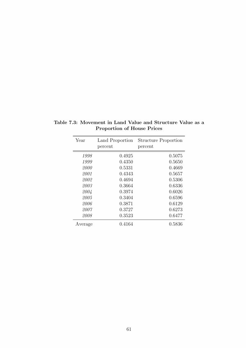
Table 7.3: Movement in Land Value and Structure Value as aProportion of House Prices

Year Land Proportion Structure Proportionpercent percent

1998 0.4925 0.50751999 0.4350 0.56502000 0.5331 0.46692001 0.4343 0.56572002 0.4694 0.53062003 0.3664 0.63362004 0.3974 0.60262005 0.3404 0.65962006 0.3871 0.61292007 0.3727 0.62732008 0.3523 0.6477

Average 0.4164 0.5836

61

Chapter 8

Significance of Other Land and Structure Quality

Characteristics

The aim of this chapter is to construct more accurate price indexes by accounting

for additional housing characteristics, in an attempt to create better quality adjust-

ments and decrease unit value bias. Including other important price-determining

characteristics is also a more parsimonious model improvement tool to using linear

splining of house prices. The additional price-determining characteristics tested in

this section are the number of rooms, the availability of parking. the quality of

inside and outside maintenance performed to the house, quality of garden storage

space, and non-linear effects of land and structure size.

I expect structure quality to increase as the quality of parking availability increases.

The parking availability term is included in the regression in a multiplicative fashion

to capture the assumption it is subject to the same depreciation that influences the

entire structure component. I also assume parking availability only affects structure

quality with no effect on land quality, which seems reasonable as the parking spaces

involve garages which are additions to the houses’ structure component. My model

captures an increase in the price of structure per metre squared as the quality of

available parking increases by running the regression in Equation 8.1;

V tn = αtLtn + β1p

t(1− δtAtn)(1 + λP tn)Stn + εtn (8.1)

My regression results support this intuition and indicate that parking availability

has a statistically significant impact on structure price per square metre at the 1%

significance level for all time periods. The model has an adjusted R2 of 0.9804. My

results in Table 8.1 indicate that the availability of parking has a significant economic

impact on housing price. More specifically, increasing average available parking

quality by 1 unit (as defined in the data section) increase the average structure

price per square metre by 53.9 Euros.

62

Table 8.1: Hedonic Regression Prices with Parking Included

Year Land price Structure price Depreciation Parking priceper m2 per m2 rate (%) per unit

1998 0.1786 0.5066 0.1143 0.0702(0.0067) (0.0179) (0.0079) (0.0119)

1999 0.1663 0.6008 0.1078 0.1008(0.0079) (0.0205) (0.0082) (0.1282)

2000 0.2508 0.5480 0.1122 0.0978(0.0095) (0.0197) (0.0076) (0.0123)

2001 0.2286 0.7265 0.1268 0.0634(0.0091) (0.0194) (0.0064) (0.0094)

2002 0.2781 0.6116 0.1004 0.0355(0.0097) (0.0171) (0.0065) (0.0084)

2003 0.2082 0.6613 0.0750 0.0629(0.0092) (0.0177) (0.0064) (0.0089)

2004 0.2468 0.7470 0.1019 0.0321(0.0090) (0.0162) (0.0056) (0.0069)

2005 0.2211 0.7720 0.0771 0.0441(0.0095) (0.0171) (0.0054) (0.0064)

2006 0.2555 0.7968 0.1060 0.0371(0.0099) (0.0163) (0.0051) (0.0068)

2007 0.2668 0.8116 0.1068 0.0152(0.0083) (0.0150) (0.0049) (0.0062)

2008 0.2497 0.7370 0.0844 0.0335(0.0130) (0.0195) (0.0068) (0.0090)

Average 0.2319 0.6837 0.1012 0.0539

63

I also test whether the quality of inside maintenance to a house increases structure

value. This maintenance is assumed to include renovations and basic fixations that

experience the same depreciation effects as the overall structure component, and are

assumed to only affect the structure component of the house. Including this variable

involves running the regression in Equation 8.2;

V tn = αtLtn + β1p

t(1− δtAtn)(1 + θMI tn)(1 + λP tn)Stn + εtn (8.2)

The regression results support my intuition at the 1% significance level for all time

periods, shown in Table 8.2. The model has an adjusted R2 of 0.9813. Including

inside maintenance to the regression has an economically significant impact on house

prices, where structure price increase by 110.14 Euros per unit increase in inside

maintenance quality. Note that the structure price per square metre reported in

Table 8.2 is significantly lower on average, reflecting the idea that a lot of this value

increase is being captured by the inside maintenance variable.

Performing similar methods, I test outside maintenance quality, number of bath-

rooms, number of toilets, and garden storage quality. Each variable is included in a

similar fashion to parking, where it is added as a multiplicative term to the land or

structure price per square metre. Garden storage quality and outside maintenance

quality are assumed to only affect land quality. The number of bathrooms and

number of toilets are assumed to only affect structure quality, where I also assume

that depreciation affects bathrooms and toilets at the same rate it changes overall

house structure value. Overall, including these variables in the hedonic regressions

indicated they are statistically and economically insignificant in the final builder’s

model at the 5% significance level. The number of rooms and number of bathrooms

are likely to be insignificant as a majority of their effect is captured by including

the structure floor space area. Garden storage quality is not found to be significant

due to the relatively homogenous nature of garden storage facilities for Assen houses.

I now test for a non-linear relationship between the price-determining characteristics

and house prices. The first effect I test is between building size and transaction price

by including a land parcel size squared variable, L2tn. This highlights the idea that

increasing the building size won’t continue to increase the price indefinitely, and at

some turning point will start to have a diminishing effect on price. Similarly, the

age of the building may be squared to account for the idea that price changes non-

linearly with changes in age. I test for this specification’s statistical and economic

significance by including the variable A2tn. My regression results indicate that land

64

Table 8.2: Hedonic Regression Prices with Inside Maintenance Included

Year Land price Structure price Depreciation Parking price Inside Maintenanceper m2 per m2 rate (%) per unit Quality per unit

1998 0.1787 0.1638 0.0927 0.0601 0.2609(0.0064) (0.0516) (0.0091) (0.0112) (0.1189)

1999 0.1657 0.4192 0.0983 0.0970 0.0553(0.0078) (0.0660) (0.0092) (0.0127) (0.0278)

2000 0.2496 0.4064 0.1056 0.0936 0.0460(0.0095) (0.0563) (0.0081) (0.0122) (0.0236)

2001 0.2280 0.5119 0.1202 0.0604 0.0551(0.0090) (0.0645) (0.0068) (0.0093) (0.0227)

2002 0.2774 0.2906 0.0868 0.0308 0.1442(0.0094) (0.0510) (0.0070) (0.0082) (0.0467)

2003 0.2069 0.4432 0.0634 0.0598 0.0625(0.0091) (0.0529) (0.0071) (0.0087) (0.0218)

2004 0.2394 0.4559 0.0885 0.0261 0.0854(0.0088) (0.0488) (0.0060) (0.0065) (0.0226)

2005 0.2144 0.5479 0.0660 .0431 0.0544(0.0096) (0.0558) (0.0061) (0.0062) (0.0184)

2006 0.2525 0.4980 0.0938 0.0328 0.0798(0.0096) (0.0512) (0.0055) (0.0065) (0.0210)

2007 0.2667 0.2613 0.0857 0.0139 0.2733(0.0077) (0.0573) (0.0053) (0.0058) (0.0874)

2008 0.2406 0.4344 0.0712 0.0348 0.0946(0.0129) (0.0726) (0.0074) (0.0087) (0.0376)

Average 0.2291 0.403 0.0884 0.0502 0.1101

65

squared has a statistically significant (but economically meaningless impact) since

the coefficient on land squared is on average -0.0001 during the 11 year period.

I now compare my results to those obtained by Diewert et al (2015). In their paper,

Diewert et al (2015) reason that as the number of rooms increases, the quality

of the structure will increase. Thus, the price per meter squared of a structure

should increase as the number of rooms increases. This is tested using the following

regression in Equation 8.3;

V tn = αtLtn + β1p

t(1− δtAtn)(1 + ΩRtn)Stn + εtn (8.3)

Diewert et al (2015) find that including the number of rooms in the regression has

an economically and statistically significant impact on structure value. Including

the number of rooms variable in this manner captures the effect of the number of

rooms taking out the effect of room number captured by including the structure floor

space variable. My regression results are inconsistent with the finding of Diewert

et al. I find that the number of rooms variable is significant at the 1% significance

level in some years and insignificant at the 10% significance level for other years.

Although this contradicts the findings of Diewert et al (2015), it makes intuitive

sense because the majority of the impact of number of rooms is being captured

by structure floor space area and inside house maintenance. This is supported by

the findings of Palmquist (1984) that indicate structure size does not have a linear

effect on house prices (where Palmquist finds that construction costs don’t increase

proportionally as structure size increases and the number of rooms effect should be

fully captured by structure floor space).

Finally, I note that Coulson (1992) finds significant volatility in large structure prices

in the US, indicating that the structure price should be non-constant structure price

per square metre. Testing the non-linearity of the impact of structure floor space

would provide a useful extension to this thesis but is not considered here, since I

assuming the additive decomposition framework holds for determining house value.

8.1 Final Builder’s Model

The final builder’s model used to calculate land value and structure value for Assen

housing based on the regression results in this section is shown by Equation 8.4;

66

V tn = αt(1− γLtn)Ltn + β1p

t(1− δtAtn)(1 + θMI tn)(1 + λP tn)Stn + εtn (8.4)

Running this regression on the Assen data set and aggregating results, I find that

including land parcel size (in a non-linear fashion), structure floor space, age of

a structure, and parking availability quality explain 88% of house price variation.

The model has an adjusted R2 of 0.9822. The final regression output is shown in

Table 8.3. Note land squared price per square metre is not reported in the table

but is included in the regression, and has a coefficient of -0.0001 with a standard

error of 0.0000 on average. Thus, including land squared in the model improves

the functional form of the model (and yields different regression results as shown in

Table 8.3).

Note that the Appendix contains the LR test results between the basic builder’s

model and final builder’s model. The result indicates that adding parking, inside

maintenance quality, and land squared have a statistically significant improvement

on the model’s fit.

The land and structure values are shown in Figure 8.1 and indicate that land and

structure equally account for approximately 50% of house value over time. The

proportion of house value explained by land value over time has stayed relatively

constant. This result makes intuitive sense and indicates that land policy in Assen

has managed to maintain land and structure value constant over time (adjusting for

inflation), which is part of their policy objective in regards to housing affordability.

Before proceeding to the user cost analysis, I will mention a key limitation of this

thesis’ coverage. An economically significant improvement to this thesis would be to

evaluate and adjust for the desirability of land using fixed effects analysis, where a

probability measure of flood risk in The Netherland’s is applied and combined with

data on how close a city is to water and key environmental hazards. I ignore these

effects in my thesis, noting key limitations in the Assen data set.

67

Table 8.3: Hedonic Regression Prices for Final Builder’s Model

Year Land price Structure price Depreciation Parking price Inside Maintenanceper m2 per m2 rate (%) per unit Quality per unit

1998 0.2384 0.1895 0.1079 0.0669 0.4801(0.0153) (0.0549) (0.0111) (0.0137) (0.3597)

1999 0.2787 0.2524 0.1190 0.1277 0.1041(0.0174) (0.0655) (0.0114) (0.0185) (0.0558)

2000 0.2696 0.3771 0.1085 0.0967 0.0525(0.0213) (0.0628) (0.0089) (0.0133) (0.0272)

2001 0.3363 0.3852 0.1394 0.0658 0.0766(0.0170) (0.0656) (0.0082) (0.0112) (0.0334)

2002 0.3138 0.2465 0.0926 0.0340 0.1779(0.0203) (0.0553) (0.0079) (0.0089) (0.0650)

2003 0.2974 0.3502 0.0771 0.0606 0.0866(0.0224) (0.0572) (0.0085) (0.0099) (0.0321)

2004 0.2992 0.3762 0.0973 0.0259 0.1131(0.0191) (0.0539) (0.0069) (0.0071) (0.0325)

2005 0.3551 0.3788 0.0809 .0358 0.0965(0.0232) (0.0612) (0.0075) (0.0073) (0.0339)

2006 0.3360 0.4155 0.1042 0.0358 0.0971(0.0195) (0.0534) (0.0064) (0.0073) (0.0273)

2007 0.4136 0.3693 0.1065 0.0111 0.3917(0.0195) (0.0579) (0.0068) (0.0069) (0.1748)

2008 0.4000 0.3654 0.0928 0.0347 0.1820(0.0365) (0.0813) (0.0102) (0.0104) (0.0907)

Average 0.2291 0.3205 0.1024 0.0541 0.1689

Figure 8.1: Final Builder’s Model: Land Value and Structure Valueversus House Value

68

Chapter 9

Investigating the User Cost of Residential Property

I use an asset-market model on sales of detached residential properties to analyse

short-run and long-run housing affordability in Assen. This utilises Poterba’s (1984)

user cost of capital framework. Comparison with expected empirical results from

the literature will also be discussed.

9.1 Additional Data for User Cost of Housing

Calculation

The following subsections delve into additional data required to calculate the user

cost of housing in Assen. Note that the data listed here are only estimates and

further investigation using more accurate data is highly advised.

9.1.1 Marginal Income Tax Rate

I will quickly introduce The Netherland’s income tax system to provide context in

which to analyse these user cost figures. The full deductibility of mortgage payments

from an individual’s personal income tax remains a key incentive for investing in

The Netherlands housing market. The Netherlands’ has a partly progressive tax

rate which has become less progressive from 1998 to 2008. Historically, individuals

in The Netherland’s highest income tax bracket had a marginal income tax rate of

72%. This has gradually decreased over time, down to 60% in 1990 and 52% in

2001. The marginal income tax brackets in 2014 were 33.5%, 42% and 52%.

Note in Poterba’s (1984) framework that property tax is deducted from an owner

occupier’s taxable income. The property tax rates used in my analysis are already

adjusted for this deduction and therefore, I do not include an explicit marginal

income tax term in my user cost model.

69

Figure 9.1: 10-year interest rate on Netherland’s government bonds

9.1.2 Risk-Free Interest Rate

The risk-free interest rate measures the interest an owner-occupier of housing

forgoes on the dwelling’s market value. The risk-free interest rate is obtained from

the annual interest rate on Netherland’s government bonds (this data is readily

accessible from the FRED database). The long-term interest rate is 4.36% on

average over this time period and fluctuates only marginally on an annual basis

between 3.3% and 5.3%, as shown in Figure 9.1.

9.1.3 Property Tax Rate

An owner-occupier of real estate incurs a property tax liability arising from

contractual ownership of the piece of real estate. In The Netherlands, the property

tax rate is determined on a local municipality level. Taxation can vary significantly

between different regions and over time. There are also complications in calculating

the rate of property tax, as there is an additional taxation system for different

infrastructural support systems such as water-level management, water cleaning,

and waste management that complements the standard land tax rate.

The property tax rate in Assen is estimated using an adjustment to the property

tax levy on owner-occupied housing in Amsterdam in 2014 and 2015. Using these

tax levies, I compute the growth rate between these time periods and interpolate a

property tax growth rate for the period 1998 to 2008 in Amsterdam on an annualised

basis. I assume that the Assen property tax rate is equal to the property tax rate in

Amsterdam, and that the Assen property tax rate follows the same growth pattern

70

Figure 9.2: Assen Property Tax Rate

and fluctuations over time. Using Amsterdam data is desirable as data on real estate

rates and costs are more readily available for Amsterdam relative to smaller cities

in The Netherlands like Assen.

The property tax rate for Assen fluctuates between 0.06795% and 0.07605% of WOZ

value, with an average property tax rate of 0.07200% of WOZ value. The WOZ value

is a term used in The Netherlands to compute the amount of house value that is

assessable for local and provincial taxation purposes.

The graph of the property tax rate in Assen is provided in Figure 9.2. The property

tax rate appears to decrease linearly from 1998 to 2008, indicating a decrease in

property tax costs for owner-occupiers.

9.1.4 Maintenance and Depreciation Costs

The maintenance and depreciation rate per annum for property in Assen is estimated

to be 2.5% per annum. I assume this value based on the annual depreciation rate

used by Himmelberg et al (2005), who based their motivation for assuming this value

by referring to analysis conducted on housing depreciation rates by Harding et al

(2004). The same depreciation rate has been assumed elsewhere in the literature,

such as by Syed and Hill (2012).

71

Figure 9.3: Expected Capital Gains for Assen Residential Housing

9.1.5 Risk Premium of Home Ownership

The risk premium of owning a unit of housing relative to renting is assumed to be

2.5% per annum, using the framework and assumptions of Flavin and Yamashita

(2002). The same rate has been assumed in the literature, including papers by

Himmelberg et al (2005) and Syed and Hill (2012).

Flavin and Yamashita (2002) construct an asset allocation line of portfolio inclusive

of housing, which allows comparison of the bond-to-stock ratio with the proportion

of financial assets in stocks to measure the risk premium.

Note this estimate for risk premium may be too high because it does not factor

in the insurance value of owning a house in hedging risk. Nevertheless, choosing

an alternative value has been found to have little effect on user cost over time

(Himmelberg et al, 2005).

Th risk premium measure could be improved in future analysis by generalising the

model to allow the relative risk of home ownership versus renting to vary over time.

9.1.6 Expected Capital Gains

The expected house price appreciation is constructed from 1 year ahead forecasted

expected capital gains in Assen (which are calculated using the house prices from

my data set). The fluctuations in these expected appreciations is provided in Figure

9.3. The expected capital gains fluctuate between 1.8% and 6.1% per annum with

an average of 3.56% per annum. This expected capital gain rate seems reasonable

72

given the strong growth in The Netherland’s property sector and strong population

density growth in The Netherlands.

9.2 Applying Poterba’s Framework to Assen Housing

The user cost of housing for a given time period t is calculated using Equation 9.1;

UCt = rt + αt + δt + γt − βt (9.1)

where;

− UCt = per dollar cost of owning one unit of housing for period t,

− rt = 10-year interest rate on Netherland’s government bonds for period t,

− αt = property tax rate for period t,

− δ = maintenance and depreciation rate for housing,

− γ = risk premium of owning a unit of housing relative to renting, and

− βt = 1-year forecasted expected capital gain for Assen.

It is appropriate to keep the values δ and γ constant since they are just expectations.

These variables are kept in the regression. An alternative approach would be to take

these variables out of the equation (since they are constant over time) and analyse

percentage changes in user cost over time. However, the focus of this thesis is to

find evidence of changes in housing affordability over time in levels terms, which

provides justification to keep these variables in the user cost calculation.

Note that mortgage interest payments are accounted for in this framework since

mortgage interest payments on owner-occupied housing in The Netherlands is fully

deductible.

Using this framework, I calculate the theoretical equilibrium user cost of capital

shown in Figure 9.4. The theoretical equilibrium user cost of housing decreased

from 1999 to 2006 from 5.9% to 2%, before increasing back up to 6.1% by 2008.

Rents in the social rental sector tend to be 70% of the maximum rent allowed for

a dwelling. The responsibility for the affordability of housing is shared between the

73

Figure 9.4: Theoretical Equilibrium User Cost of Housing

government and the social rental sector (Haffner and Boumeester, 2010). As there

are not many dwellings with a market rent, this may be an indication of the market

rent that is actually achievable on average. This may also be the effect of the large

number of dwellings on the market that are offered for social rent and effectively

subsidised via rent regulation.

Housing allowances influence the gross rent level for households in the rental sector.

The average housing allowance in 2006 was 148 Euros per month for each recipient

(Ministry of VROM, 2007).

9.3 Theoretical versus Market User Cost

The user cost of housing over one year at equilibrium should equal the cost of renting

housing over the year. This equilibrium condition is expressed in Equation 9.2;

Rt = utPt (9.2)

The theoretical market equilibrium is where user cost = rentprice

. In words, the user

cost is equal to the inverse of the price-rent ratio. The framework is interpreted as

follows. If actual market rent exceeds theoretical market rent, than home ownership

is more affordable relative to renting a house. This occurs where the market rent

is greater than the theoretical gross market rent. If market rent is represented by

MRt, than this relationship can be defined by Equation 9.3;

MRt > p UC (9.3)

74

Figure 9.5: Assen: Market Rent for Housing

The actual market rent data is obtained using the growth rate of the Harmonised

Index of Consumer Prices: Actual Rentals for Housing for Netherlands, and applying

this to the monthly rent observed in Amsterdam. This rental series is shown in

Figure 9.5.

The disequilibrium between the theoretical user cost and market user cost is provided

in Figure 9.6. Home ownership has better affordability relative to renting in The

Netherlands over time. Home ownership has also become relatively cheaper to

renting over time. Interestingly, disequilibrium in the market increases from 2003

to 2008. This reflects increasing costs in The Netherlands rental market, which is

consistent with the government’s increase in the gross rent level for renters and the

abolition of in subsidies provided to housing associations to provide social rental

housing.

It is interesting to note that rents for social housing are significantly lower than

for private housing in The Netherlands. Thus, when applying the framework to

other countries the user cost will need to be adjusted for comparison.

Also, the gross rent level for renters is controlled by each municipality. This makes

it difficult to accurately measure the difference between social housing rents and

market rents. The government has regulated rents since World War 2, and has

75

Figure 9.6: Theoretical versus Market User Cost of Housing

enforced a maximum rent cut-off of 615 Euros per month. The average rental level

in The Netherlands in 2002 was 508 Euros per month, with the average rent in the

social rental sector equal to 353 Euros per month in 2002.

Since 2002, the government has decreased regulation in the housing by allowing

landlords to increase gross rent by a larger amount. It is likely rent levels have

increased since 2002, but there is a lack of certainty on this matter due to the lack

of publicly available information on these trends. Furthermore, the government’s

decreased regulation has benefited the private sector by significantly increasing

rental income for landlords providing social and private housing, but has come

at a cost to The Netherland’s governments financial stability by increasing the

government’s financial burden for providing housing allowances.

76

Chapter 10

Implications for the Real Estate Sector

The use of the additive decomposition framework to decompose house prices into

land and structure components has implications for central banks in measuring

land and capital stocks more accurately. Regulators will also need to understand

and account for this framework, and commercial developers will be able to use

the decomposition to provide additional housing sector information to their clients.

This will continue the trend in the industry towards revamping hedonic price index

methodologies, such as Core Logic. A major consideration for regulators is how to

go about backtracking price indexes to obtain accurate measures for market updates

and national accounts, and to understand the value of the different components of

housing.

The paper finds that the Netherlands’ government has been effective in using real

estate market policies to slowly decrease the financial burden on the government

over time. The social housing sector has been decentralised and is now funded by

housing associations. The government has also provided housing associations greater

flexibility to prioritise housing issues at a localised level. Additionally, housing

associations are able to access the Central Housing Fund established in 1995 to help

financially weak associations. The decreased regulation of the social rental sector

has changed the role of housing associations. In the 1980s, housing associations

focused on increasing social housing stock and providing moderate rental yields

for good quality housing. There was great expansion of housing stock across The

Netherlands and little competition for middle income earners.

Since 2000, housing associations have started to set rental yields near the equilibrium

market level. Housing associations now have greater access to capital markets.

Combined with historically low interest-rates in the Dutch economy, this has resulted

in housing associations significantly increasing new construction of owner-occupied

houses. As housing has become more accessible, middle income households have

continued to leave the rental market to the owner occupier market. This is supported

by my user cost results which indicate home ownership is more affordable relative to

renting. This trend in housing market movement and the changing role of housing

associations is an area for future research.

77

New roles are being considered for housing associations including environmental

management around dwellings, providing houses for non-traditional clients such as

the elderly and students, and provide facilities such as schools and shops. Addi-

tionally, many housing associations have begun to invest at the neighbourhood level

by offering extra services like insurance, neighbourhood centres and environmental

maintenance. This improves the quality of life in these neighbourhoods and keeps

property prices high. A key research area is to analyse how housing associations

have reacted to market changes.

As demonstrated in this paper, houses prices have appreciated quite quickly in Assen.

This appreciation trend is consistent across The Netherlands, which has resulted

in significant housing affordability issues for low income earners and first-home

buyers. Decreasing the gap between the rental market and owner-occupier market

is currently a key concern for policymakers. This was addressed in June 2006 in the

Vision for Housing Market policy announcements, which involves subsidised loans

to first-home buyers (Dekker, 2006). This raises an important policy consideration

for municipal governments and housing associations in how to set the gross market

rent. This can be answered by using econometric methods to predict the drift in

important variables used to measure house prices and user cost, with a focus on

the impact of economic changes on home ownership affordability for low-income

earners. This is crucial as low income earners represent 30% of all households in

The Netherlands. Low income earners in this context are identified as individuals

with a taxable income below 33,000 Euros.

One major challenge for the Dutch housing sector in the coming decades is urban

renewal control. A lot of housing stock was built in the post-war period and needs

to be replaced and refurbished. To renew housing stock, this will require an urban

renewal program which will be expensive in the short-run and will require prudent

financial management.

Another policy area to consider is the government’s taxation policy. The government

has kept mortgage interest payments for owner occupation fully deductible from

income tax. Although this has helped the government achieve it’s national policy

of promoting home ownership over social renting, it is likely mortgage interest tax

relief on owner-occupied dwellings has pushed house prices in The Netherland’s up

quite significantly. Renters spent on average 15.5% of disposable income on housing

in 1982, and this grew to 21% by 1994. At the same time, buying a house has

comparatively cheap due to record-low mortgage interest rates. This has created a

78

massive tenure shift of households with moderate and higher income to buy housing

and this effect persists today.

There are also implications from financial market changes. There are now a greater

variable of mortgage products available, which has resulted in record high debt levels

in The Netherlands. Gross expenditure is expected to change in the Netherlands,

as land supply becomes less elastic and house prices continue to rise. There is

uncertainty over how this will influence competition in The Netherlands real estate

sector. A further area to investigate the lag in supply of new dwellings in Assen in

response to housing shortages, and how this influences housing affordability.

Sustaining the financial position of housing associations is a key policy issue for

The Netherlands government. To develop the real estate sector, a system that

allows housing associations to self-regulate needs to be established. The Ministry for

Housing in The Netherlands has also identified improving internal supervision and

developing benchmarks to better manage the performance of housing associations,

and as an alternative to self-regulation.

Finally, the user cost results can be improved by explicitly factoring in subsidised

rents for social housing (which are significantly lower than for private housing).

Since these rents are controlled by each municipality, it is difficult to accurately

measure the difference between social and market rents. Obtaining better data for

rent levels in the Netherlands is a key priority,

79

Chapter 11

Concluding Remarks

This thesis runs hedonic regressions on the sales of detached houses in Assen

from 1998 to 2008 through an additive decomposition framework. The additive

decomposition framework models house prices into it’s land and structure values

separately. This provides greater understanding of house price dynamics and has

potential application in the commercial sector and for statistical agencies in creating

quality-adjusted price indexes. This thesis has found evidence that structure value

has increased more quickly than land value over time.

The theoretical rent calculated under Poterba’s user cost framework is lower than

actual market rent reflecting disequilibrium in the housing sector, where home

ownership has become more affordable relative to renting. This provides evidence

of a potential ’bubble’ in Assen’s rental market.

The thesis’ findings have direct policy implications for the government in achieving

it’s goal of creating a competitive market for residential housing, and improving

the qualitative aspects of housing. An example is reconsideration of social housing

subsidies, zoning laws, and the NMG Scheme. The additive decomposition also has

many potential uses in the commercial sector and for regulators to gain a more

accurate insight into house price dynamics.

80

Chapter 12

Appendix

Likelihood Ratio (LR) test of Basic Builder’s Model and the Final Builder’s Model:

The LR test compares the goodness of fit between the basic builder’s model and

the final builder’s model. The ratio can be interpreted as how many times more

likely the data is under one model than the other. The LR test is calculated using

Stata and involves evaluating the following expression;

LR = −2lnL(m1)

L(m2)= 2(ln(m2)− ln(m1)) (1)

where;

− m1:

V tn = αtLtn) + βt(1− δtAtn)Stn + εtn (2)

− m2:

V tn = αt(1− γLtn)Ltn + β1p

t(1− δtAtn)(1 + θMI tn)(1 + λP tn)Stn + εtn (3)

− H0: m1 fits the data

− H1: m2 fits the data

− Assumption: m1 nested in m2

− LR χ2(3) = 3085.97

− Probability > χ2 = 0.0000

81

References

Anselin, L. (1988). ‘Spatial Econometrics: Methods and Models,’ Dordrecht:

Kluwar Academic Publishers, 1-283.

Basu, S. & Thibodeau, T. (1998). ‘Analysis of Spatial Autocorrelation in House

Prices,’ Journal of Real Estate Finance and Economics, 17(1), 61-85.

Boelhouwer, P., Haffner, M., Neuteboom, P, & De Vries, P. (2004). ‘House prices

and income tax in the Netherlands: an international perspective,’ Housing Studies,

19(3), 415 - 432.

Atkinson, S.E. & Crocker, T.D. (1987). ‘A Bayesian approach to assessing the

robustness of hedonic property value studies’, Journal of Applied Econometrics,

2(1), 27-45.

Bostic, R.W., Longhofer, S. D., & C. L. Redfearn. (2007). ‘Land Leverage:

Decomposing Home Price Dynamics,’ Real Estate Economics, 35(2), 183-208.

Boelhouwer, P.J. (2005). ‘The incomplete privatization of the Dutch housing market:

exploding house prices versus falling house-building output,’ Journal of Housing and

the Built Environment, 20, 363-378.

Bourassa, S.C., Haurin, D.R., Haurin, J.L., Hoesli, M., & Sun, J. (2009). ‘House

Price Changes and Idiosyncratic Risk: The Impact of Property Characteristics,’

Real Estate Ecconomics, 37(2), 259-278.

Case, B., Pollakowski, H. O., & Wachter, S. M. (1991). ‘On Choosing Among

House Price Index Methodologies,’ American Real Estate and Urban Economics

Association, 19(3), 259-472.

Case, K. E., Quigley, J.M., & Shiller, R.J. (2005). ‘Comparing Wealth Effects:

82

The Stock Market versus the Housing Market’, 5(1), 1534-1563.

CBS Statline. (2016). ‘GDP, production and expenditures; value, Quarterly

National Accounts’.

CBS Statline. (2014). ‘Bevolkingsontwikkeling; regio per maand [Population

growth; regions per month]’.

Clapp, J. M. (1980). ‘The elasticity of substitution for land: The effects of

measurement errors,’ Journal of Urban Economics, 8, 255-263.

Chow, G.C., & Niu, L. (2010). ‘Demand and supply for residential housing in

urban China,’ Journal of Financial Research, 44(1), 1-11.

Daniel, V.E., Florax, R.J.G.M, & Rietveld, P. (2009). ‘Floods and Residential

Property Values: A Hedonic Price Analysis for the Netherlands,’ Built Environment,

35(4), 563-576.

Davis, M.A., & Heathcote, J. (2007). ‘The price and quantity of residential land in

the United States,’ Journal of Monetary Economics, 54(8), 2595-2620.

Davis, M. A., & Palumbo, M. G. (2008). ‘The price of residential land in large

U.S. cities,’ Journal of Urban Economics, 63, 352-384.

De Boor, C. (1979). ‘A Practical Guide to Splines,’ New York: Springer-Verlag.

Diewert, W.E. (2011). ‘Alternative Approaches to Measuring House Price Inflation,’

Journal of Economic Literature Classification Numbers, 10(10).

Diewert, W. E. (2003). ‘Hedonic regressions: A review of some unresolved issues,’

University of British Columbia: Department of Economics, 1-40.

Diewert, W. E. (1974). ‘Intertemporal Consumer Theory and the Demand for

Durables,’ Econometrica, 42, 497-516.

Diewert, W.E. (1974). ‘Application of duality theory,’ Frontiers of Quantitative

Economics, 2, 106-171.

Diewert, W.E. & Wales, T.J. (1992). ‘Quadratic spline models or producer’s supply

83

and demand functions,’ International Economic Review, 33, 705-722.

Diewert W. E., de Haan, J., & Hendricks, R. (2015). ‘Hedonic Regressions and

the Decomposition of a House Price Index into Land and Structure Components,’

Econometric Reviews, 34(1-2), 106-126.

Diewert, W. E., Heravi, S., & Silver, M. (2007). ‘Hedonic Imputation versus Time

Dummy Hedonic Indexes,’ IMF Working Paper, 07(234), Washington D.C.

Drake, L. (1993). ‘Modelling UK house prices using cointegration: an application

of the Johansen technique,’ Applied Economics, 25(9), 1255-1228.

Flavin, M., & Yamashita, T. (2002). ‘Owner-occupied housing and the composition

of the household portfolio,’ The American Economic Review, 92(1), 345-362.

Fox, K. J. (1998). ‘Non-parametric estimation of technical progress,’ Journal of

Productivity Analysis, 10(3), 235-250.

Francke, M. K. & Vos, G. A. (2004). ‘ The hierarchical trend model for property

valuation and local price indices’, Journal of Real Estate Finance and Economics,

28, 179-208.

Friedman, J. H. & Silverman, B. W. (1989). ‘Flexible Parsimonious Smoothing

and Additive Modeling,’ Technometrics, 31(1), 3-21.

Glaeser, E. L., & Gyourko, J. (2003). ‘The impact of building restrictions on housing

affordability,’ Economic Policy Review, 9, 21-39.

Gyourko, J., Mayer, C., & Sinai, T. (2013). ‘Superstar Cities,’ American Economic

Journal: Economic Policy, 5(4), 167-199.

Gyourko, J., Deng, Y., & Wu, J. (2015). ‘Evaluating the Risk of Chinese Housing

Markets: What We Know and What We Need to Know,’ NBER Working Paper

Series, 21346, 531-543.

Haffner, M.E.A., and Boumeester, H.J.F.M. (2010). ‘The affordability of housing in

the Netherlands: An increasing income gap between renting and owning?,’ Housing

Studies, 25(6), 799-820.

84

Harding, J.P., Rosenthal, S.S., & Sirmans, C.F. (2004). ‘Depreciation of Housing

Capital and the Gains from Homeownership,’ working paper, Syracuse University.

Hatzvi, E. & Otto, G. (2008). ‘ Prices, Rents and rational speculative bubbles

in the Sydney housing market,’ Economic Record, 84(267), 405-420.

Hill, R.J. (2004). ‘Comparing Price Indexes Across Countries and Time: The Case

of the European Union,’ American Economic Review, 94(5), 1379-1410.

Hicks, J. R. (1939). ‘The Foundations of Welfare Economics’, The Economic

Journal, 49(196), 696-712.

Hill, R. J. & Syed, I. A. (2012). ‘Hedonic price-rent ratios, user cost, and departures

from equilibrium in the housing market,’ Regional Science and Urban Economics,

56, 60-72.

Hill, R. J., Melser, D., & Syed, I. A. (2008). ‘Flexible Spatial and Temporal Hedonic

Price Indexes for Housing in the Presence of Missing Data,’ School of Economics

Discussion Paper.

Himmelberg, C., Mayer, C., & Sinai, T. (2005). ‘Assessing High House Prices:

Bubbles, Fundamentals and Misperceptions,’ Journal of Economic Perspectives,

19(4), 67-92.

Holly, S., Pesaran, M.H., & Yamagata, T. (2010). ‘A spatio-temporal model of

house prices in the US,’ Journal of Econometrics, 158(1), 160-173.

Koev, E., and Santos Silva, J.M.C. (2008). ‘Hedonic Methods for Decomposing

House Price Indices into Land and Structure Components,’ Unpublished paper,

Department of Economics, University of Essex, England.

Hulchanski, D.J. (1995). ‘The concept of housing affordability: six contemporary

uses of the housing expenditure-to-income ratio,’ Housing Studies, 10, 471-491.

Kakes, J. & Van Den End, J.W. (2004). ‘Do stock prices affect house prices?

Evidence for the Netherlands,’ Applied Economics Letters, 11(12), 741-744.

Pain, N. & Westaway, P. (1997). ‘Modelling structural change in the UK housing

market: a comparison of alternative house price models,’ Economic Modelling, 14(4),

85

587-610.

Pakes, A. (2003). ‘A Reconsideration of Hedonic Price Indexes with an Application

to PC’s,’ The American Economic Review, 93, 1576-11593.

Poirier, D. J., & Garber, S. G. (1974). ‘The Determinants of Aerospace Profit

Rates, 1951 - 1971,’ Southern Economic Journal, 41, 228-238.

Poterba, J. M. (1984). ‘Tax subsidies to owner-occupied housing: An asset-market

approach,’ The Quarterly Journal of Economics, 99(4), 729-752.

Poterba, J.M. (1992). ‘ Taxation and Housing: Old Questions, New Answers’,

NBER Working Paper Series, 3963, 1-15.

Priemus, H. & Fieleman, F. (1997). ‘Social rented housing: Recent changes in

western Europe - Introduction,’ 421-425.

Rambaldi, A.N., McAllister, R.R.J., & Fletcher, C.S. (2015). ‘Decoupling land

values in residential property prices: smoothing methods for hedonic imputed price

indices,’ Technical report, Discussion Papers Series 549, School of Economics, The

University of Queensland, Australia.

Rubin, D. B. (1987). ‘Multiple Imputation for Nonresponse in Surveys,’ New York:

Wiley, 1-239.

Shiller, T. (2006). ‘Housing: Boom or Bubble?,’ Business Review Q4, 9-18.

Shiller, R.J. (2007). ‘Understanding recent trends in house prices and home

ownership,’ No. w13553. National Bureau of Economic Research, 2007.

Van Ewijk, C., Konink, M., Lever, M., & de Mooij, R. (2006). ‘Economische effecten

van aanpassing fiscale behandeling eigen woning,’ Den Haag: CPB.

Vandevyvere, W. & Zenthofre, A. (2012). ‘The Housing Market in the Netherlands,’

European Commission, 457.

Verbrugge R. (2008). ‘The Puzzling Divergence of Rents and User Costs, 1980-

2004,’ Review of Income and Wealth, 54(4), 671-699.

86

Wu, J., Deng, Y., & Liu, H. (2013). ‘House price index construction in the nascent

housing market: The case of China,’ Journal of Real Estate Finance and Economics,

48, 522-545.

87