University of Leipzig - Wirtschaftswissenschaftliche ... · PDF filemarginal cost. Incentive constraint ful–lled by a ... w on the output Harald Wiese (University of Leipzig)

Advanced MicroeconomicsHidden action

Harald Wiese

University of Leipzig

Harald Wiese (University of Leipzig) Advanced Microeconomics 1 / 42

Hidden action

1 Introduction2 The principal-agent model3 Sequence, strategies, and solution strategy4 Observable e¤ort5 Unobservable e¤ort6 Special case: two outputs7 More complex principal-agent structures


Introduction

The agent is to perform some task for the principal, the asymmetry ofinformation occurs after the agent has been employed

Problem: the output is assumed to be a function of both the agent�se¤ort and chance

Since the e¤ort is not observable, the payment to the agent (asspeci�ed in the contract) is a function of the output, but not of e¤ort

Principalchooses thecontract.

Naturechoosesthe output.

Agent decideswhether to acceptthe contract.

Principalagent model

Agent decideson effort level.


Introduction

The principal-agent problem is described as the principal�smaximization problem subject to two conditions:

participation constraintincentive compatibility

Principal-agent models often assume that the principal is risk neutraland the agent risk averse;

Pareto optimality requires that the agent does not bear any risk.

However, in order to incite the agent not to be lazy, it may benecessary to have the agent bear some risk


The principal-agent model

De�nition (Principal-agent problem)

A tuple Γ = (fP,Ag , E ,X , (ξe )e2E , c , u�is called a principal-agent

problem where

P is the principal; A is the agent,

E = R+ is the agent�s action set (his e¤ort level),

c : E ! R is the agent�s cost-of-e¤ort function,

X is the output set or the set of net pro�ts,

ξe is the probability distribution on X generated by e¤ort level e,

the principal�s nonprobabilistic payo¤ is given by

x � w , with x 2 X , wage rate w 2 R,

the agent�s nonprobabilistic payo¤ is given by

w � c (e)the agent�s reservation utility is u 2 R.


Sequence, strategies, and solution strategy

The principal-agent problem is modeled as a four-stage game

1 The principal chooses a wage function which speci�es the wage as afunction of the output. This wage function is also called a contract

2 The agent decides whether to accept the contract3 The agent decides on his e¤ort level4 Nature chooses the output and thus the payo¤s for both principal andagent

De�nition (Strategies)

Let Γ be a principal-agent problem. The principal�s strategy is a wagefunction sP = w : X ! R. The agent�s strategy is a functionsA : SP ! fy, ng � E , where y means ("yes" or "accept") and n ("no" or"decline") and refers to the agent�s participation decision. sA is sometimes

written as�sfy, ngA , sEA

�with sfy, ngA (sP ) 2 fy, ng and sEA (sP ) 2 E .


Sequence, strategies, and solution strategy

The principal can foresee the agent�s reaction to any wage function heo¤ers

We look for a subgame-perfect equilibrium

Our solution strategy to the principal-agent problem focuses on thee¤ort level of an agent who accepts a contract

Imagine that the principal aims for an e¤ort level b 2 E , the principalmaximizes his payo¤ under two conditions:

The agent needs to prefer accepting the contract and exerting e¤ortlevel b to not accepting the contractThe agent needs to prefer e¤ort level b to any other e¤ort level e 2 E


Observable e¤ort

The principal can directly observe the agent�s e¤ort or the principalobserves the output and can deduce the e¤ort unequivocallyThe principal can propose a payment scheme with domain E or X(we assume domain X )Assume that the principal wants the agent to choose some e¤ort levelb 2 E ; his maximization problem is

maxw(x (b)� w (x (b)))

subject to the side conditions

w (x (b))� c (b) � u, participation c.w (x (b))� c (b) � w (x (e))� c (e) for all e 2 E , incentive c.

There is no need to give more to the agent than the reservation utility;

w (x (b)) = u + c (b) (1)

is the minimal wage that ful�lls the participation constraintHarald Wiese (University of Leipzig) Advanced Microeconomics 8 / 42

Observable e¤ort

Thus, the optimal e¤ort chosen by the principal (!) is

e� = argmaxe(x (e)� (u + c (e)))

where e� is obtainable (in good-natured problems) by

dxde|{z}

marginal output

!=

dcde|{z}

marginal cost

.

Incentive constraint ful�lled by a boiling-in-oil contract:

w (x) =�u + c (e) , x = x (e)�∞ x 6= x (e)

The payo¤s are x (e�)� u � c (e�) for the principal and u for theagentThe sum of the payo¤s is x (e�)� c (e�) and hence the payo¤ thatthe principal could achieve if he were his own agent


Unobservable e¤ortThe model

We assume that the principal knows the probability distribution ξegenerated by any e¤ort level e 2 EIn general, this knowledge plus the speci�c output is not su¢ cient toreconstruct the e¤ort level itself

Principal bases his wage payments w on the output



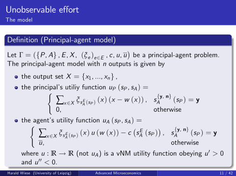
De�nition (Principal-agent model)

Let Γ = (fP,Ag ,E ,X , (ξe )e2E , c , u, u�be a principal-agent problem.

The principal-agent model with n outputs is given by

the output set X = fx1, ..., xng ,the principal�s utiliy function uP (sP , sA) =(

∑x2X ξsEA (sP )(x) (x � w (x)) , sfy, ngA (sP ) = y

0, otherwise

the agent�s utility function uA (sP , sA) =(∑x2X ξsEA (sP )

(x) u (w (x))� c�sEA (sP )

�, sfy, ngA (sP ) = y

u, otherwise

where u : R ! R (not uA) is a vNM utility function obeying u0 > 0and u00 < 0.



The agent�s utility function uA is somewhat special; the cost of e¤ortcan be separated from the utility with respect to the wage earnings

We now try to solve the principal-agent model. The two sideconditions for action b 2 E are

∑x2X

ξb (x) u (w (x))� c (b) � u, participation c.

∑x2X

ξb (x) u (w (x))� c (b)

� ∑x2X

ξe (x) u (w (x))� c (e) for all e 2 E ,incentive c.


Unobservable e¤ortApplying the Lagrangean method to the participation constraint

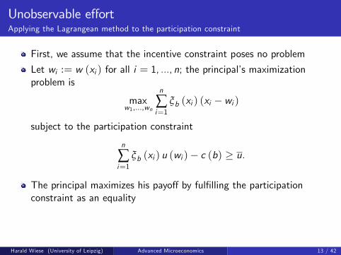
First, we assume that the incentive constraint poses no problem

Let wi := w (xi ) for all i = 1, ..., n; the principal�s maximizationproblem is

maxw1,...,wn

n

∑i=1

ξb (xi ) (xi � wi )

subject to the participation constraint

n

∑i=1

ξb (xi ) u (wi )� c (b) � u.

The principal maximizes his payo¤ by ful�lling the participationconstraint as an equality



The Lagrangean of this problem is

L (w1,w2, ...,wn,λ)

=n

∑i=1

ξb (xi ) (xi � wi ) + λ

n

∑i=1

ξb (xi ) u (wi )� c (b)� u!.

The Lagrange multiplier λ > 0 indicates the additional payo¤ accruingto the principal if the participation constraint is relaxed. Reducing thereservation utility by one unit increases the principal�s payo¤ by

λ = �duPdu

which is not quite, but basically correct



The partial derivatives with respect to wi (i = 1, ..., n) yield

∂L∂wi

= �ξb (xi )| {z }wage payments increase

with probability ξb(xi )

+ λ ξb (xi ) u0 (wi )| {z }

participation constraint

is relaxed

!= 0.

Bad news: An increase of wi (i.e., in case of output xi ) by one unitreduces the expected pro�t by ξb (xi ) because the wage payments areincreased by one unit with probability ξb (xi )Good news: A wage increase eases the participation constraint byξb (xi ) u

0 (wi ); multiply by λ to obtain the pro�t increaseThe wages are the same for all outputs:

u0 (wi )!=1λ

the risk averse agent is not exposed to any riskHarald Wiese (University of Leipzig) Advanced Microeconomics 15 / 42

Unobservable e¤ortApplying the Kuhn-Tucker method to the incentive constraint

A constant wage is not optimal if the incentive constraint is bindingThe principal�s optimization problem leads to the Lagrangean

L (w1,w2, ...,wn,λ, µ)

=n

∑i=1

ξb (xi ) (xi � wi )

+λ

n

∑i=1

ξb (xi ) u (wi )� c (b)� u!(participation constraint)

+µe 0

∑x2X

ξb (x) u (w (x))� c (b)�

∑x2X

ξe 0 (x) u (w (x))� c�e 0�!!

+µe 00

∑x2X

ξb (x) u (w (x))� c (b)�

∑x2X

ξe 00 (x) u (w (x))� c�e 00�!!

+... (all the other incentive constraints)



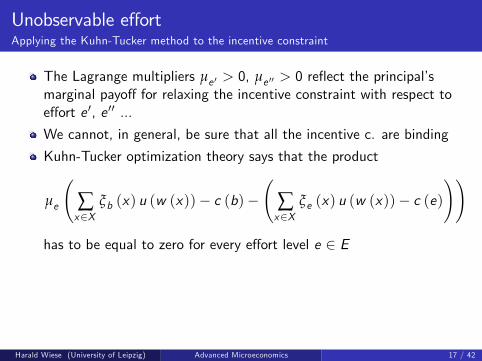
The Lagrange multipliers µe 0 > 0, µe 00 > 0 re�ect the principal�smarginal payo¤ for relaxing the incentive constraint with respect toe¤ort e 0, e 00 ...

We cannot, in general, be sure that all the incentive c. are binding

Kuhn-Tucker optimization theory says that the product

µe

∑x2X

ξb (x) u (w (x))� c (b)�

∑x2X

ξe (x) u (w (x))� c (e)!!

has to be equal to zero for every e¤ort level e 2 E



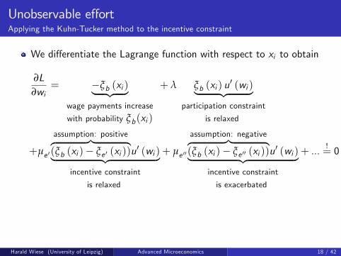
We di¤erentiate the Lagrange function with respect to xi to obtain

∂L∂wi

= �ξb (xi )| {z }wage payments increase

with probability ξb(xi )

+ λ ξb (xi ) u0 (wi )| {z }

participation constraint

is relaxed

+µe 0

assumption: positivez }| {(ξb (xi )� ξe 0 (xi ))u

0 (wi )| {z }incentive constraint

is relaxed

+ µe 00

assumption: negativez }| {(ξb (xi )� ξe 00 (xi ))u

0 (wi )| {z }incentive constraint

is exacerbated

+ ...!= 0



Assume the special case of two e¤ort levels b and e

The above maximization condition implies (after some reshu ing)

u0 (wi )!=

ξb (xi )λξb (xi ) + µe (ξb (xi )� ξe (xi ))

=1

λ+ µeξb (xi )�ξe (xi )

ξb (xi )

.

Assume µe > 0 and ξb (xi ) > ξe (xi ). Then

wage wi should be relatively high in order to give the agent anincentive to choose b rather than eformally, u0 (wi ) is smaller for µe > 0 than for µe = 0Sketch a concave vNM utility function so that you see why a small u0

implies a large wi .


Special case: two outputsThe model

Two output levels, x1 and x2, and two actions, e and b

We assume

Output x2 is higher than output x1 : x1 < x2,b makes x2 more likely than e : ξb (x2) > ξe (x2),b is the principal�s preferred action

ExerciseDo x1 < x2 and ξb (x2) > ξe (x2) imply that the principal aims for brather than e?



So far:

principal �xes wages w = w (x) andvNM utility u (w)

From now on:

principal �xes vNM utility levels andw (u) is the wage level necessary in order to give vNM utility u to theagent

If u is concave, w = u�1 is convex.



The principal who aims at e¤ort level b obtains maximal payo¤

π (b) = maxu1,u2

ξb (x1) [x1 � w (u1)] + ξb (x2) [x2 � w (u2)]

subject to the two side conditions

ξb (x1) u1 + ξb (x2) u2 � c (b) � u, p. c.ξb (x1) u1 + ξb (x2) u2 � c (b) � ξe (x1) u1 + ξe (x2) u2 � c (e) , i. c.

Solving for u2 yields

u2 � u+c (b)ξb (x2)

� ξb (x1)ξb (x2)

u1, participation c.

u2 � u1 + c (b)�c (e)ξb (x2)�ξe (x2)

, incentive c.


Special case: two outputsThe indi¤erence curves

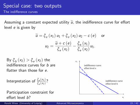
Assuming a constant expected utility eu, the indi¤erence curve for e¤ortlevel e is given by

eu = ξe (x1) u1 + ξe (x2) u2 � c (e) or

u2 =eu + c (e)ξe (x2)

� ξe (x1)ξe (x2)

u1.

By ξb (x2) > ξe (x2) theindi¤erence curves for b are�atter than those for e.

Interpretation of ξe (x1)ξe (x2)

?

Participation constraint fore¤ort level b? 1u

2u

indifference curveeffort level e

indifference curveeffort level b


Special case: two outputsThe indi¤erence curves

1u

2u

participation linefor effort level b

incentive linefor effort level b

( )( )2x

bcu

bξ+

( ) ( )( ) ( )22 xx

ecbc

eb ξξ −−

c (b)� c (e) > 0 � > incentive line above 45�-line

utiliy di¤erence u2 � u1 does not fall below c (b)�c (e)ξb (x2)�ξe (x2)

utility levels u1 and u2 have to be chosen inside the highlighted area


Special case: two outputsThe principal�s iso-pro�t lines

The principal�s pro�t

π (u1, u2) = ξb (x1) [x1 � w (u1)] + ξb (x2) [x2 � w (u2)] ,

The slope of the iso-pro�t lines is given by

du2du1

= �∂π∂u1∂π∂u2

= � ξb (x1)w0 (u1)

ξb (x2)w 0 (u2)

negatively sloped because w 0 (u1) and w 0 (u2) are positivethe nearer the iso-pro�t lines are to the origin, the higher the pro�tthey indicate


Special case: two outputsThe principal�s iso-pro�t lines

An increase in u1 leads toan increase in w 0 (u1)(convexity of w),

a decrease in u2 (negativeslope of the iso-pro�tline)and hence

a decrease in w 0 (u2)(convexity of w)

� > absolute value of theslope increasesu1 = u2 � > iso-pro�t line�sslope: � ξb (x1)

ξb (x2)

1u

2u

isoprofit lines

°45


If we do not need to worry aboutincentive compatibility, ...


Special case: two outputsSolving the principal-agent problem

1u

2u


isoprofit lines

°45


cb � ce � > u1 +c (b)�c (e)

ξb (x2)�ξe (x2)� u1

The incentive constraint does not prevent the �rst-best solution (i.e.,the solution when there is no asymmetric information)


Special case: two outputsSolving the principal-agent problem

1u

2u


isoprofit lines

°45


cb > ce � > u1 +c (b)�c (e)

ξb (x2)�ξe (x2)> u1

Optimal risk sharing at u1 = u2 is not possible

Second-best solution (taking asymmetric information into account)


Special case: two outputsSolving the principal-agent problem: example

From Milgrom/Roberts (1992, pp. 200-203):

We have two outputs 10 and 30.

The agent has two e¤ort levels, 1 and 2. E¤ort level 2 makes output30 more likely than e¤ort level 1 :

E¤ort level Output x = 10 Output x = 30e = 1 ξ1 (10) = 2/3 ξ1 (30) = 1/3e = 2 ξ2 (10) = 1/3 ξ2 (30) = 2/3

The agent is risk averse with vNM utility functionu (w , e) =

pw � (e � 1) . The reservation utility is u = 1.

The principal has the pro�t function π given by π (w , x) = x � w .In case of unobservable e¤ort, the principal�s wage function is givenby w (10) � wl , w (30) � wh.


Special case: two outputsSolving the principal-agent problem: observable e¤ort (questions)

If the principal aims for e = 1, what is his optimal wage function?

If the principal aims for e = 2, what is his optimal wage function?

Should the principal aim for e¤ort level 1 or 2?


Special case: two outputsSolving the principal-agent problem: observable e¤ort (answers)

If the principal aims for e = 1, he needs to take care of the participationconstraint, only: p

w � (e � 1) � u.The wage rate w = 1 ful�lling this constaint automatically takes care ofthe incentive problem.



In case of observable e¤ort, it is easy to force e = 2. The wage rate ofwe=2 = 4 guarantees the participation constraint

pwe=2 � (2� 1) � 1.

The incentive constraint ispwe=2 � (2� 1) �

pwe=1 � (1� 1) which

can be rewritten as

pwe=1 � p

we=2 � 1=

p4� 1

= 1.

Thus, the wage function

w =�4, e = 21, e = 1

is optimal.



e = 1 and w = 1 implies the expected pro�t

π (e = 1) =23� 10+ 1

3� 30� 1

=473

while e = 2 and w = 4 leads to

π (e = 2) =13� 10+ 2

3� 30� 4

=583

>473.

The principal should aim for e = 2.


Special case: two outputsSolving the principal-agent problem: unobservable e¤ort for e=2 (questions)

Write down the participation constraint in terms ofpwl and

pwh.

Write down the incentive constraint in terms ofpwl and

pwh.

Depict the two constraints by puttingpwl on the abscissa and

pwh

on the ordinate.

Determine wl and wh !


Special case: two outputsSolving the principal-agent problem: unobservable e¤ort for e=2 (answers)

In case of unobservability, the wage needs to be a function of output, note¤ort. wl is the wage for the low output 10 and wh is the wage for thehigh output 30.The agent�s participation constraint for the high e¤ort 2 is

13u (wl , 2) +

23u (wh, 2)

=13(pwl � 1) +

23(pwh � 1)

=13pwl +

23pwh � 1

� 1,

or pwh � 3�

12pwl .



The incentive constraint for e¤ort 2 rather than 1 is

13pwl +

23pwh � 1

=13u (wl , 2) +

23u (wh, 2)

� 23u (wl , 1) +

13u (wh, 1)

=23pwl +

13pwh,

which can also be written as

pwh � 3+

pwl .



constraints squareroot

7.pdflw

hw

631

4

3

1

2participation linefor effort level 2

incentive line



From the �gure, we learn that the principal should not pay a positive wageto the agent in case of x = 10. We have

pwh = 3 and

pwl = 0 or the

wage function

w =�9, x = 300, x = 10

.

The principal�s pro�t is

π (e = 2) =13� (10� 0) + 2

3� (30� 9)

=523.


Special case: two outputsSolving the principal-agent problem: unobservable e¤ort

Is the principal�s pro�t higher for e = 1 than for e = 2?Very similar to the case of observable e¤ort, if the e¤ort level 1 is aimedfor, the incentive constraint is no problem. We know that w = 1 ful�llsthe participation constraint and leads to the pro�t 473 . By

523 >

473 the

principal should go for e = 2. Note 583 >

523 , i.e., observability leads to a

higher pro�t. After all, e = 2 is a second-best solution, only.


Special case: two outputsSolving the principal-agent problem: unobservable e¤ort (question di¤erent problem)

What is the optimal contract for these probabilities:

E¤ort level Output x = 10 Output x = 30e = 1 ξ1 (10) = 2/3 ξ1 (30) = 1/3e = 2 ξ2 (10) = 0 ξ2 (30) = 1


Special case: two outputsSolving the principal-agent problem: unobservable e¤ort (answer di¤erent problem)

The new probabilities reduce the principal�s uncertainty. The high e¤ortprecludes the low output. Here, a boiling-in-oil contract is optimal:

w =�4, x = 300, x = 10

ful�lls the participation constraint because the agent has the (expected)payo¤

p4� (2� 1) = 1 = u. E¤ort level e = 1 leads to the expected

utility 23

p0+ 1

3

p4 = 2

3 < 1.


More complex principal-agent structures

We consider two-tier principal-agent structures. Tirole (1986) pointsto three-tier structures

principal supervisor agentproduction unit manager foreman workerregulation government regulating authority �rmPhD procedure faculty council professor PhD stud.professorship ministry of educ. dean/rector professor

time, competence or cost e¢ ciency

Does the supervisor act in the principal�s interests? Sometimes,

the agent�s achievements re�ect on the supervisor,the supervisor and the agent collude against the principal,secret side payments play a role.


Documents

University of Leipzig - Wirtschaftswissenschaftliche ... · PDF filemarginal cost. Incentive constraint ful–lled by a ... w on the output Harald Wiese (University of Leipzig)