University of Groningen

Robust Feature Detection and Local Classification for Surfaces Based on Moment AnalysisClarenz, Ulrich; Rumpf, Martin; Telea, Alexandru

Published in:Default journal

IMPORTANT NOTE: You are advised to consult the publisher's version (publisher's PDF) if you wish to cite fromit. Please check the document version below.

Document VersionPublisher's PDF, also known as Version of record

Publication date:2004

Link to publication in University of Groningen/UMCG research database

Citation for published version (APA):Clarenz, U., Rumpf, M., & Telea, A. (2004). Robust Feature Detection and Local Classification for SurfacesBased on Moment Analysis. Default journal.

CopyrightOther than for strictly personal use, it is not permitted to download or to forward/distribute the text or part of it without the consent of theauthor(s) and/or copyright holder(s), unless the work is under an open content license (like Creative Commons).

Take-down policyIf you believe that this document breaches copyright please contact us providing details, and we will remove access to the work immediatelyand investigate your claim.

Downloaded from the University of Groningen/UMCG research database (Pure): http://www.rug.nl/research/portal. For technical reasons thenumber of authors shown on this cover page is limited to 10 maximum.

Download date: 19-10-2018

Robust Feature Detection andLocal Classification for Surfaces

Based on Moment AnalysisUlrich Clarenz, Martin Rumpf, and Alexandru Telea

Abstract—The stable local classification of discrete surfaces with respect to features such as edges and corners or concave and

convex regions, respectively, is as quite difficult as well as indispensable for many surface processing applications. Usually, the feature

detection is done via a local curvature analysis. If concerned with large triangular and irregular grids, e.g., generated via a marching

cube algorithm, the detectors are tedious to treat and a robust classification is hard to achieve. Here, a local classification method on

surfaces is presented which avoids the evaluation of discretized curvature quantities. Moreover, it provides an indicator for

smoothness of a given discrete surface and comes together with a built-in multiscale. The proposed classification tool is based on local

zero and first moments on the discrete surface. The corresponding integral quantities are stable to compute and they give less noisy

results compared to discrete curvature quantities. The stencil width for the integration of the moments turns out to be the scale

parameter. Prospective surface processing applications are the segmentation on surfaces, surface comparison, and matching and

surface modeling. Here, a method for feature preserving fairing of surfaces is discussed to underline the applicability of the presented

approach.

Index Terms—Surface classification, surface processing, edge detection, nonsmooth geometry.

�

1 INTRODUCTION

FEATURE detection is known to be an indispensable tool inimage processing. Features such as edges and corners

have to be classified in a stable way to enable edgepreserving image denoising [19], [1], [25] and robustsegmentation of image subdomains bounded by edges[18], [2], [25]. Correspondingly, the local classification ofsurfaces, in particular the detection of edge and cornerfeatures or the distinction of concave and convex areas onthe surface, turns out to be an important ingredient formany surface processing applications. Indeed, some appli-cations are:

. Surface fairing: A given initial, noisy surface issmoothed, while edges on it are simultaneouslypreserved or even enhanced (cf. [23], [8], [4]).

. Mesh decimation: A given surface mesh is simplifiedwhile edge features are preserved (cf. [26], [11]).

. Surface segmentation: Identification of homogeneousregions, indicated by characteristics such as con-vexity and concavity, or bounded by feature lines.

. Surface matching: Surfaces are reduced to a skeletonof features lines to enable a better comparison.

In image processing, a straightforward identification of

edges can be based on an evaluation of the image gradient.

A sufficiently large gradient is supposed to indicate anedge. Alternatively, a frequently considered edge indicatoris the Canny edge indicator, which searches for extrema ofthe second derivatives in the gradient direction [6].Furthermore, the structure tensor (cf. [24]) enables a robustclassification of edges and edge directions in images. Onsurfaces, gradients are no more natural objects for theidentification of intrinsic surface characteristics. Here, thecanonical quantity for the detection of edges is the curvaturetensor, in the case of codimension 1, represented by thesymmetric shape operator. An edge is supposed to beindicated by one sufficiently large principle curvature andthe corresponding principle curvature direction is perpendi-cular to the edgeon the surface. Thismethod iswell-suited forsmooth objects. Curvature evaluation for discrete surfacescan be based on the algorithm proposed by Moreton andSequin [17]. In particular, in surface processing, curvatureevaluation is used to detect important features [4], [23], [14],[7]. Another method of computing the curvature on discretedata sets is given by [4], where the surface is locally projectedonpolynomial graphs over the tangent space. In [7], themeancurvature is defined as the first variation of the areafunctional. This approach is closely related to the minimalsurface algorithm by Pinkall and Polthier [20]. Furthermore,in [16], discrete curvatures are computed, where the discreteGaussian curvature is based on the quotient of a localspherical image and the corresponding local surface area.Curvature is an object which comes along with smoothness.Consequently, on discrete surfaces, we can separate areas oflow curvature from nonsmooth areas. Nevertheless, wecannot obtain information about the structure of the non-smooth part. For that reason, curvature estimation requires atedious treatment and is unstable on irregular surfaces or

516 IEEE TRANSACTIONS ON VISUALIZATION AND COMPUTER GRAPHICS, VOL. 10, NO. 5, SEPTEMBER/OCTOBER 2004

. U. Clarenz and M. Rumpf are with the Institute fur Mathematik, DuisburgUniversity, Germany. E-mail: {clarenz, rumpf}@math.uni-duisburg.de.

. A. Telea is with the Department of Mathematics and Computer Science,Eindhoven University of Technology, The Netherlands.E-mail: alext@win.tue.nl.

Manuscript received 30 Apr. 2003; revised 19 Dec. 2003; accepted 6 Apr.2003.For information on obtaining reprints of this article, please send e-mail to:tvcg@computer.org, and reference IEEECS Log Number TVCGSI-0030-0403.

1077-2626/04/$20.00 � 2004 IEEE Published by the IEEE Computer Society

on surfaces perturbed by noise. In addition, discretecurvature evaluation is a local process without a scaleand therefore very noise sensitive (see [16, Fig6(c)]).

Here, in contrast to the curvature-based approach forsurface classification, we propose a novel set of surfaceclassification criteria based on local zero and first moments.This approach is related to the structure tensor approach forimages [24] and provides a stable way to distinguishsmooth regions from the vicinity of edges and corners onsurfaces. Furthermore, it allows us to robustly extractinformation on the geometry close to, or even on a featuresingularity (cf. Section 3). In [22], moments have alreadybeen applied for the computation of skeletons from distancefunction singularities in 2D and 3D. For an approach toskeletons of 3D point clouds representing surfaces, we referto [15]. In this paper, we generalize the techniquespresented in [22] and [5] to yield a general tool for theclassification of feature singularities. A subsequent advan-tage of our method is that it comes along with an embeddedscale factor that allows a simple and natural way fordetecting important surface structures at or above a user-selected scale. In addition, this paper provides a detailedquantitative analysis of the local surface classifiers whichwe believe to be the backbone of the observed robustness inthe application. Here, in particular, the different scalings ofthe zero moment in smooth and nonsmooth situations,respectively, and the corresponding scaling and theeigenvalues of the first moment are derived.

We apply the presented surface classification tool for anumber of fairly distinct triangular surfaces of differentorigin, complexity, and resolution. Finally, as an applicationin actual surface processing, we consider edge preservingsurface fairing. Hence, we apply an anisotropic geometricdiffusion. Here, moment-based local classification is used todistinguish edges from smooth surface areas and to identifyedge directions on the surface. For the correspondingbackground and literature, we refer to [4], [5].

The paper is organized as follows: In Section 2, we recallhow surfaces may be classified using curvature informa-tion. In Section 3, the local moment analysis is presented.We give proofs of the fact that the zero moment scalesquadratically in smooth domains of a surface, where itscales only linearly in nonsmooth domains (cf. Theorem 2and Theorem 4) and that the scaling of the first moment isquadratically in smooth and nonsmooth areas. Indeed, todistinguish smooth from nonsmooth regions based on firstmoments requires a comparison of the eigenvalues of thefirst moment (cf. Theorem 3 and Theorem 5). Furthermore,we discuss the implementation on triangle meshes. InSection 4, we compare curvature and moment classificationand demonstrate experimentally the robustness of theapproach. The application in surface fairing is describedin Section 4.2. Finally, in Section 5, we draw conclusions.

Notation. Let us summarize notations and conventionswe are going to use in the sequel. We consider a parametermanifold M which essentially fixes the topological type ofimmersed surfaces x : M ! IRdþ1. Hence, the actual surfaceis xðMÞ. With a slight misuse of notation, we will denotethe surface x again by M. The parameter on M is denotedby �. By T �M, we denote the tangent space at � and by T M

the tangent bundle of M. For immersions x, the differentialDx induces, canonically, a metric on M via the relationgðv; wÞ ¼ DxðvÞ �DxðwÞ which holds for all v; w 2 T M.Here, the scalar product in IRm is denoted by �. Incoordinates, we obtain gij ¼ gð@i; @jÞ. Suppose

RM f dA

denotes the usual integral of a function f over M. Thus,the area element dA is given by

ffiffiffiffiffiffiffiffiffiffidet g

pd�, where g ¼ ðgijÞij

is the metric tensor corresponding to gð�; �Þ. Integration overM leads to the L2-scalar product of L2-functions f; g on M:ðf; gÞ :¼

RM f � g dA. We will make use of the gradient rM

and the divergence divM on the manifold. For a function fon M, the gradient rMf 2 T �M in � 2 M is defined bygðrMf; wÞ ¼ d

dt fðcðtÞÞjt¼0, where cðtÞ is a curve on M withcð0Þ ¼ � and _ccð0Þ ¼ w. Furthermore the divergence isdefined as the corresponding dual differential operator. Inparticular

RM divMv � dA ¼ �

RM gðv;r�Þ dA. The manifolds

M are assumed to be oriented and the normal mapping willbe denoted by n : M ! Sd, where d is the dimension of themanifold M. This enables us to define the shape operatorS : T �M ! T �M by gðST �Mw; vÞ :¼ @wn �DxðvÞ. The traceof the shape operator is the classical mean curvatureh ¼ trST �M. We often write S ¼ ST �M if a misunderstand-ing is ruled out. The Laplacian divM gradM is denoted by�M. Finally, let us from now on use Einstein summationconvention.

2 A REVIEW OF CURVATURE-BASED LOCAL

SURFACE CLASSIFICATION

In this section,webriefly recall howto locally classify surfacesbased on curvature analysis. The quantity for the detection ofhighly curved surface areas—namely, edges—is the curva-ture tensor: In the codimension 1 case, it is represented bythe symmetric shape operator ST �M. An edge is supposed tobe indicated by one sufficiently large eigenvalue of ST �M.The main drawback of this approach is that it involvesderivatives of “noisy” data, which is usually a riskyenterprise. In particular, in the interesting case of surfaceswith sharp edges, these quantities are not even defined onthe actual surface.

Thus, we have to stabilize the evaluation of the shapeoperator. This can either be done by a straightforward“geometric Gaussian” filter, which turns out to be a shorttime-step � ¼ �2=2 of mean curvature motion (for details cf.[4], [9]) or by local L2 projection of the surface onto quadraticpolynomial graphs. Let us denote this prefiltered surface byM�. Hence, for stability reasons, we compute a shapeoperator ST �M�

onM�. Here, the parameter � either indicatesthe “geometric Gaussian” filter-width or the size of theneighorhood, which we take into account for the local L2

projection [21]. Let us emphasize that we are able to reducenoise by this filter operator. But, we might also removefeatures in a hard to predict way. Now, we introduce, foreverypoint onM�, a classification tensora

�T �M�

. It is supposedto be a symmetric, positive definite, linear mapping on thetangent space T �M�. Let us suppose that w1;�; w2;� are theprincipal directions of curvature—the orthogonal eigendir-ections of the shape operator—and �1;�; �2;� the principlecurvatures—the corresponding eigenvalues. Then, wedefine the tensor a�T �M�

in the basis fw1;�; w2;�g as follows:

CLARENZ ET AL.: ROBUST FEATURE DETECTION AND LOCAL CLASSIFICATION FOR SURFACES BASED ON MOMENT ANALYSIS 517

a�T �M�¼ G �1;�ð Þ 0

0 G �2;�ð Þ

� �; ð1Þ

where the function G is given by GðxÞ :¼ 11þðx=�Þ2 . Here, �

serves as a user-defined threshold parameter which

classifies the significance of surface features. Hence, a point

is supposed to belong to an edge if there is one principal

direction of curvature on M� with large curvature com-

pared to �. If the second principal curvature is small w.r.t.

�, we consider the first direction as being orthogonal to an

edge on the surface. At corners, both principal curvatures of

M� are large. Summarizing this, our tensor leads to the

following surface classification:

. Smooth areas are characterized by a�T �M�� diag½1; 1�.

. Edges are defined by a�T �M�� diag½1; 0�. In this case,

the edge direction is given by w2;� and we assumej�1;�j >> j�2;�j.

. Corners are defined by a�T �M�� diag½0; 0�.

As a simple edge indicator, we can use the functionCcurv� ðxÞ ¼ tr a�T �M�

. Depending on the threshold parameter�, edges and corners are given by Ccurv� ðxÞ < 1. However, theabove classifier encounters serious problems on noisy dataor data containing features (e.g., edges) at several spatialscales (cf. Section 4).

Finally, let us mention that we can make use of thisclassification tensor as a diffusion tensor for surface fairing.Generalizing the algorithm introduced by Dziuk [10] formean curvature flow, we can define an anisotropicgeometric diffusion process which smoothes the surface inregions being classified as smooth and preserves edges onthe surface. In addition, we can allow smoothing along anedge. The corresponding generalized mean curvature flowis given by the following equation:

@tx� divMða�T �M�rMMxÞ ¼ 0:

For a more detailed discussion of this type of equation, werefer to Section 4.2 and to [4]. This approach generalizes theimage processing methodology presented and discussed byPerona and Malik [19], Alvarez et al. [1], and Weickert [24].Let us mention that our approach here differs fromKimmel’s method [13], where denoising of textures onsurfaces is discussed, whereas we consider the denoising ofthe surface itself.

3 MOMENT-BASED SURFACE ANALYSIS

In the following, we will introduce and discuss local surfaceclassification based on zero and first order surfacemoments. This will, in particular, allow us to robustlydistinguish smooth regions from the vicinity of edges on thecurve or surface. To begin with, we introduce thecorresponding definitions:

Definition 1. For an embedding x : M ! IRdþ1, the zeromoment is given by the barycenter M0

� ðxð�ÞÞ; � 2 M, ofxðMÞ \B�ðxð�ÞÞ, where B�ðxð�ÞÞ is the Euclidean �-ball inIRdþ1 centered at xð�Þ:

M0� ðxð�ÞÞ ¼ �

ZB�\M

x dA:

The parameter � is called the scanning width. Furthermore, the

first moment is defined as:

M1� ðxð�ÞÞ

¼ �Z

B�\Mðx�M0

� ðxð�ÞÞÞ � ðx�M0� ðxð�ÞÞÞ dA;

where y� z :¼ ðyizjÞi;j¼1;...;dþ1.

Due to the definition via local integration, the zero and the

first moment are expected to be robust with respect to noise.

To study the effectiveness of our moment-based classifiers,

we next examine their behavior on smooth (Section 3.1),

respectively, nonsmooth (Section 3.2) surfaces.

3.1 Smooth Surface Case

We first show that a locally smooth surface is characterized

by a quadratic scaling of the zero moment shift n� ¼M0

� ðxð�ÞÞ � xð�Þ and the first moment M1� ðxð�ÞÞ. Here, n�

plays the role of a scaled approximate normal.Indeed, for a smooth function � on a Euclidean �-ball

B�ð0Þ � IRd, we have:

�Z

B�

� ¼ �Z

B�

�ð0Þ þ r�ð0Þ � x

þ 1

2r2�ð0Þx � x dxþ oð�2Þ

¼ �ð0Þ þ 1

2�Z

B�ð0Þr2�ð0Þx � x dxþ oð�2Þ

¼ �ð0Þ þ 1

2�i�Z

B�ð0Þx2i dxþ oð�2Þ;

where the �i for i ¼ 1; . . . ; d are the eigenvalues of r2�ð0Þ.Note that, in the above equation, we used the fact that:

ZB�

r�ð0Þ � x dx ¼Xdi¼1

ZB�

@i�ð0Þxi dx

andRB�xi dx ¼ 0. Therefore, we have:

�Z

B�

�

¼ �ð0Þ þ 1

2� 1d�Z

B�ð0Þjxj2dx � trr2�ð0Þ þ oð�2Þ

¼ �ð0Þ þ cðdÞ �2��ð0Þ þ oð�2Þ;

where the dimension depending constant cðdÞ is given by

cðdÞ ¼ 1=½2ðdþ 2Þ�.Now, we consider the surface M in the vicinity of some

point � on M. In a first step, we replace the Euclidean ball

B�ðxð�ÞÞ � IRdþ1 by a geodesic ball eBB�ðxð�ÞÞ � M and

compute the barycenter eMM0� ðxð�ÞÞ of eBB�ðxð�ÞÞ. To evaluateReBB�ðxð�ÞÞ

xð�ÞdAð�Þ, we take into account normal coordinates,

i.e.,

gijð0Þ ¼ ij; @kgijð0Þ ¼ 0:

For more details on normal coordinates see e.g., the

textbook [12, p. 19]. Then, one obtains for the Laplacian

on M at xð�Þ:

518 IEEE TRANSACTIONS ON VISUALIZATION AND COMPUTER GRAPHICS, VOL. 10, NO. 5, SEPTEMBER/OCTOBER 2004

ð�M�Þðxð�ÞÞ ¼ ð@i@i�Þð0Þ ¼ ��ð0Þ: ð2Þ

Hence, for the difference eMM0� ðxð�ÞÞ � xð�Þ we get. Note that

we identify xð�Þ and xð0Þ as well as eBB�ðxð�ÞÞ and B�ð0Þ in

the chart and on the surface, respectively. Due to the choice

of normal coordinates, the Euclidean ball in IRd and the

geodesic ball on M coincide via the chart map.

eMM0� ðxð�ÞÞ � xð�Þ ¼ �

ZB�ð0Þ

x dx� xð0Þ

¼ cðdÞ�2�xð0Þ þ oð�2Þ¼ cðdÞ�2�Mxð�Þ þ oð�2Þ¼ �cðdÞ�2hð�Þnð�Þ þ oð�2Þ;

where h is the mean curvature of M. Here, we have taken

into account the classical [3] relation between the Laplace-

Beltrami operator applied to the coordinate mapping and

the mean curvature vector:

�Mx ¼ �hn:

Let us point out here that, for the Euclidean ball on the

surface B�ðxð�ÞÞ \M and for the geodesic ball eBB�ðxð�ÞÞ, we

have the relation

j jB�ðxð�ÞÞ \Mj � j eBB�ðxð�ÞÞj j ¼ Oð�dþ2Þ:

We observe an order dþ 2 instead of d due to the vanishing

first order terms @kgijð0Þ for normal coordinates. Therefore,

one can replace the geodesic ball by the Euclidean ball

without losing the corresponding scaling order.So far, we obtain:

Theorem 2. Let x : M ! IRdþ1 be an immersion. For � 2 Mconsider a ball of radius � with center xð�Þ and the �-normal

n�ð�Þ ¼ M0� ðxð�ÞÞ � xð�Þ. Then, n� scales quadratically in �

and

n�ð�Þ ¼ ��2cðdÞhð�Þnð�Þ þ oð�2Þ:

Using (2), we can give a corresponding scaling result for the

first moment. Choosing � ¼ xixj, one easily evaluates the

components of the first moment:

�Z

B�\Mxixj dA

¼ xið�Þxjð�Þ þ cðdÞ �2 �MðxixjÞ þ oð�2Þ¼ xið�Þxjð�Þ þ cðdÞ �2 ð2rMxi � rMxj

þ xj�Mxi þ xi�MxjÞ þ oð�2Þ:

Therefore, the scaling of the first moment is also quadratic:

ðM1� Þij

¼ �Z

B�\Mxixj dA��

ZB�\M

xi dA �Z

B�\Mxj dA

¼ 2 cðdÞ �2rMxirMxj þ oð�2Þ¼ 2 cðdÞ �2ð�T �MÞij þ oð�2Þ;

where �T �M is the linear projection onto the tangent space

of M at point xð�Þ. More precisely, �T �M is the matrix

representation w.r.t. the canonical basis of IRdþ1 and

ð�T �MÞij is the corresponding matrix entry. We can state:

Theorem 3. For an embedding x : M ! IRdþ1, the first moment

w.r.t. xð�Þ and scanning width � scales quadratically:

M1� ðxð�ÞÞ ¼ 2 cðdÞ �2�T �M þ oð�2Þ:

3.2 Nonsmooth Surface Case

We now discuss the case of nonsmooth surface features,

such as edges and corners. To this aim, let x : M ! IRdþ1 be

a Lipschitz continuous immersed surface, which is smooth

up to a one-dimensional subset �M. Here, �M is the edge

set on the surface. With respect to the scaling behavior of

the shift n� of the zero moment centered at x0 ¼ xð�0Þ,�0 2 �M, it suffices to assume that, for a small open domain

U ¼ Uðx0Þ � IRdþ1, the set M\ U is of cone type, i.e., x 2M\ U implies ðx� x0Þ þ x0 2 M\ U for all 2 ½0; 1Þ.This is a first order, i.e., linear approximation of the

curvilinear case. Furthermore, consider �0 such that

B�0ðx0Þ � Uðx0Þ and let �1; �2 < �0. If we assume for a

moment x0 ¼ 0, we derive from the cone property the

following identity:

��d�11

ZB�1

\Mx dA ¼ ��d

1

ZB�1

\Mx=�1 dA

¼ ��d2

ZB�2

\Mx=�2 dA ¼ ��d�1

2

ZB�2

\Mx dA;

and this leads to

��11 �Z

B�1\M

x dA ¼ ��12 �Z

B�2\M

x dA: ð3Þ

These equations are a result of the self-similarity of a cone.

For the general case, where x0 is not necessarily the origin,

we have the following result:

Theorem 4. Let x : M ! IRdþ1 be a Lipschitz continuous

embedding that is smooth on M� �M; then, for �0 2 �M,

consider a ball of radius � with center x0 ¼ xð�0Þ and

n�ð�0Þ ¼ M0� ðxð�0ÞÞ � xð�0Þ. Then, there is a vector ~nn such

that

n�ð�0Þ ¼ � ~nnþ oð�Þ:

In the case d ¼ 1, we are able to compute the length of the

above vector ~nn. This enables us to determine the apex angle

of an edge of a given curve explicitly. The corresponding

computation and result can be found in [5].Next, let us consider the first moment and consider the

following special situation for d ¼ 2:L e t D� ¼ fðx1; x2; x3Þ 2 IR3jx3 ¼ 0; x1 � 0; x2

1 þ x22 � �2g

be a semidisc in IR3. Rotating D� around the x2-axis by an

angle ’, resp. �’, we obtain two semidiscs S1� and S2

� ,

respectively. Now, we compute the first moment of the

union S ¼ S1� [ S2

� . This tensor coincides up to higher order

terms with the actual first moment M1� ðxð�ÞÞ, where xð�Þ is

contained in the singularity set �M of the Lipschitz

continuous surface, where S1� and S2

� are the two tangential

planes at xð�Þ. Here, due to the invariance of the first

moment w.r.t. translations, we assume that xð�0Þ ¼ 0. We

observe that, for �1; �2 < �, one has

CLARENZ ET AL.: ROBUST FEATURE DETECTION AND LOCAL CLASSIFICATION FOR SURFACES BASED ON MOMENT ANALYSIS 519

��21 �Z

S\B�1

x� x dA ¼ ��22 �Z

S\B�2

x� x dA:

By Theorem 4, one obtains for the zero moment M0�1

of

S \B�1 :

M0�1�M0

�1¼ �21 ~nn� ~nnþ oð�21Þ:

Hence, we obtain quadratic scaling of the first moment, as in

the smooth case.We now explicitly compute the eigenvalues of the first

moment ofS. Because of the above considerations concerning

the scaling behavior, we set � ¼ 1 as well as S11 ¼ S1, S2

1 ¼ S2,

D1 ¼ D. The two subsetsS1 andS2 are of the same area. Thus,

we can express the first moment M1ðSÞ of S by the first

moments of S1 and S2 and an additional correction term:

M1ðSÞ ¼ M1ðS1 [ S2Þ

¼ 1

4M1ðS1Þ þ 1

4M2ðS2Þ þ 1

4�Z

S1

x� x dA

�

��Z

S1

x dA��Z

S2

x dAþ�Z

S2

x� x dA

��Z

S2

x dA��Z

S1

x dA

�

¼ 1

2M1ðS1Þ þ 1

2M2ðS2Þ þ 1

4�Z

S1

x dA��Z

S1

x dA

�

��Z

S1

x dA��Z

S2

x dAþ�Z

S2

x dA��Z

S2

x dA

��Z

S2

x dA��Z

S1

x dA

�

¼ 1

2M1ðS1Þ þ 1

2M2ðS2Þ þ fTPTg;

ð4Þ

where, by TPT , we denote all tensor product terms above.

The first moment of the semidisc D in the x3-plane is

M1ðDÞ ¼1=4� ½4=ð3�Þ�2 0 0

0 1=4 0

0 0 0

0B@

1CA

¼ 0:0699 0 0

0 � ¼ 0:25 0

0 0 0

0B@

1CA:

Introducing the matrix Q ¼ diagð1; 1;�1Þ one gets

M1ðS2Þ ¼ QM1ðS1ÞQT . Analogous relations are valid for

each tensor product term of TPT in (4). Finally, by taking

into consideration these arguments, we obtain:

M1ðSÞ ¼ cos2 ’ 0 0

0 � 0

0 0 sin2 ’

0B@

1CA

þ0 0 0

0 0 0

0 0 �RS1x3 dA

� �20B@

1CA:

Because of the equation sin2 ’þ �RS1x3 dA

� �2¼ � sin2 ’, we

finally obtain:

Theorem 5. Let x : M ! IR3 be a C0;1-surface which is smooth

up to a one-dimensional set �M � M. We assume that, for

�0 2 �M, the surface xðMÞ has an edge of apex angle 2’. Inthat case, the first moment M1

� ðxð�0ÞÞ scales quadratically asin the smooth case. Furthermore, the eigenvalues of the firstmoment are �2�, �2� sin2 ’, and �2 cos2 ’ (up to higher orderterms) if � and are the eigenvalues of the first moment of D.

Let us summarize what we have obtained so far: Thezero moment shift n� on surfaces scales quadratically withrespect to the scanning width � in smooth surface areas,whereas it scales linearly in nonsmooth areas. Even thoughthe scaling behavior of the first moment in the smooth andthe nonsmooth case is identical, the eigenvalues giveadditional information on the presence of an edge and thecorresponding edge angle. This justifies the usage ofmoments as detectors for surface features. For a given,usually small, parameter �, only features larger than � willbe detected. In Section 4.1, we will derive feature classifiersbased on these results and illustrate their performance by anumber of examples.

3.3 Implementation of Zero and First MomentComputation

Above, we have treated arbitrary surfaces. In the applica-tions, we usually deal with two-dimensional, irregular,triangular grids. In the following, we will detail thediscretization of the presented local surface classificationin this case. Hence, we consider a polyhedron Mh

consisting of triangles. In our implementation, we computethe moments centered at each node of the triangulation.

Let us fix one node Xi and denote the moments by M0�;h

and M1�;h. Here, h indicates the grid size and � is, as before,

the radius of the corresponding Euclidean ball. Given this

radius �, first of all, one collects all triangles fT1; . . .Tmg of

the triangulation such that Ti \B�ðXiÞ 6¼ ;; i ¼ 1; . . .m.

This set of triangles splits into two subsets. The first one

—denoted by T o—consists of all elements with Ti \B� ¼ Ti.

The second one, T @ , is supposed to be the complement, i.e.,

Ti 2 T @ implies Ti \B� 6¼ ;. Now, we iteratively compute

the integrals �RT ox dA and �

RT ox� x dA. To this aim, we use

the following relation for averaged integrals over disjoint

sets A;B:

�Z

A[Bf ¼ jAj

jAj þ jBj �Z

A

f þ jBjjAj þ jBj �

ZB

f: ð5Þ

On each triangle of T 0, we use the following exactintegration formulas:

M0ðTiÞ ¼1

3ðX0 þX1 þX2Þ ;

�Z

Ti

x� x dA ¼ 1

3ðY0 � Y0 þ Y1 � Y1 þ Y2 � Y2Þ;

where X0; X1; X2 are the nodes of Ti and Y0 ¼ ðX0 þX1Þ=2,Y1 ¼ ðX1 þX2Þ=2, and Y2 ¼ ðX0 þX2Þ=2. For the corre-sponding computations on T @ \B�, we apply an approx-imation. For each triangle Tl 2 T @ , the intersection of thesphere @B� and the edges of the triangle consists of twopoints, denoted by P1; P2. We replace the curvilinearconnection Tl \ @B� by the line segment connecting P1 andP2. Hence, we replace Tl \B� by a polygon which we again

520 IEEE TRANSACTIONS ON VISUALIZATION AND COMPUTER GRAPHICS, VOL. 10, NO. 5, SEPTEMBER/OCTOBER 2004

can split into triangles. Now, we proceed as above usingexact integration on all these virtual triangles. Using (5), oneis able to compute the average integrals over the quad-rilaterals. Next, once again, we iteratively compute �

RT @ x dA

and �RT @ x� x dA. Finally, we get

M0�;h ¼ �

ZT o[T @

x dA

¼ jT ojjT oj þ jT @ j

M0ðT oÞ þ jT @ jjT oj þ jT @ j

M0ðT @Þ

and an analogous relation for �RT o[T @ x� x dA and achieve

M1�;h ¼ �

ZT o[T @

x� x dA�M0�;h �M0

�;h:

4 FEATURE CLASSIFICATION AND APPLICATIONS

In this section, we will derive feature detectors on surfacesand experimentally verify their robustness. We propose thefollowing two classification methods:

. zero moment classification: C0� ¼ Gðjn�j=�Þ,

. combined zero and first moment classification: C0;1� ¼Gðjn�j�min

� �maxÞ with �min; �max, the smallest and largest

eigenvalue of M1� ðxÞ.

Here, the function G is GðsÞ ¼ 1þ�s2

with suitably chosen; � > 0. The quotient �min=�max is approximatively givenby Theorem 5:

�min=�max ¼ =� cos2 ’ ¼ 0:2796 cos2 ’;

where 2’ is the apex angle as in Theorem 5. This relation for�min=�max is valid for ’ larger than 0:2726 16o. Especially,in the smooth case (’ ¼ �=2), this quotient vanishes whereit increases for decreasing ’. For ’ smaller than 16o, thequotient again tends to 0 when ’ ! 0. In this sense, verysharp features will be detected in a weaker sense as theyshould be. Nevertheless, as our experiments show, thisseems to be a theoretical detail. In real-world applications,the above observation does not play an important role andis partly compensated by the zero moment.

First, we show the classifiers on various data sets(Section 4.1) and compare the zero and first momentclassifiers with respect to robustness, detail detection, andcomputation time. In particular, it turns out that thecombined classification is performing much better. Indeed,already, for small parameters �, we obtain a robust featuredetection. Let us mention that the computational cost for asingle moment evaluation on a vertex of the surface Mh isOð�h

2Þ. Hence, the cost is large for a scanning width � whichis relatively large compared to the grid size h. As we willsee, one obtains satisfying results for typical meshes Mh

and � 3h; 4h. Finally, we present an application of theproposed detectors for surface denoising (Section 4.2).

4.1 Classification Results

At first, we test our classification in Fig. 1 on a sequence ofoctahedra with an increasing noise level. In this case, thescale, i.e., the scanning width is always the same. Fig. 2shows the detection of details on different scales choosing adifferent scanning width �. Here, the norm of the linearlyrescaled zero moment shift n�ð�Þ ¼ M0

� ð�Þ � xð�Þ is colorcoded from red (low) to green (high). Next, we consider theclassification of human cortices. Here, the focus is onvisually separating convex and concave areas of the surface,which is a difficult task due to the complicated localgeometry. Potential applications are the segmentation ofcertain domains on the cortex, analyzing the course ofdiseases as, e.g., Alzheimer’s disease, and, perspectively,the matching of different cortices.

Fig. 3 shows the classification of a human cortex usingour zero moment classifier, on the same red to greencolormap as in Fig. 2. Here, we use a slightly improvedcolor coding. To be able to distinguish sulci from gyri(“mountains and valleys” or convex and concave areas,respectively), we, in addition, consider the sign of the scalarproduct n�ð�Þ � nð�Þ, where nð�Þ is an averaged oriented

CLARENZ ET AL.: ROBUST FEATURE DETECTION AND LOCAL CLASSIFICATION FOR SURFACES BASED ON MOMENT ANALYSIS 521

Fig. 1. From left to right: zero moment classifier (top row) and combined

classifier (bottom row) for white noise perturbations of maximal

amplitudes h, 2h, 3h in normal direction (from left to right). We always

choose the scanning width � ¼ 4h.

Fig. 2. Different scales of the zero moment shift on a surface choosing

� ¼ 0:02 on the left, 0:04 in the middle, and 0:06 on the right. The

diameter of the object is scaled to 1.

Fig. 3. Human cortex classification using the zero moment shift, different

viewpoints. The scanning width is � ¼ 0:05, where the diameter of the

object is scaled to 1.

normal on the surface. The surface was generated by amarching cube algorithm and consists of approximately130,000 triangles.

Fig. 4 compares both types of surface classifications.Here, the scanning width is � ¼ 3h, where h is the averagediameter of the data set triangle cells. This corresponds to afraction of 0.015 of the object size. We notice that, by thecombined zero and first moment classification, we obtainthe best results. The zero moment classification delivers asignificantly weaker result for the same scanning width.Although, for a larger scanning width, one is able to detectthe major edges (cf. Fig. 3), the combined classifiervisualizes and separates fine structures much better.Furthermore, Fig. 5 shows a comparison of the classificationbased on moments and based on local curvature computa-tion as introduced in Section 2 (here, based on the local L2

projection onto polynomial graphs). This comparisonclearly demonstrates the robustness of the new momentbased method with respect to noise.

In Fig. 6, subsequent examples are shown using bothclassifiers C0� and C0;1� The scanning width is � ¼ 4h in allcases. As in the previous examples, the zero momentclassifier C0� is only able to detect coarser scale features. Thebest results are obtained by the combined zero and firstmoment classifier C0;1� . In all applications listed so far, weused ¼ 0:1, whereas � was set to 5 for the zero momentclassifier, 100 for the first moment classifier, and 20 for thecombined classifier, respectively. The computation of theclassifiers took around 7 seconds for a mesh of 269,000triangles on a Pentium 4 PC at 1.7 GHz.

4.2 Edge Preserving Surface Fairing

As an application of our local surface classification insurface processing, we consider the fairing of surfaces

based on anisotropic geometric diffusion. Our model

preserves edges and in addition enables tangential smooth-

ing along edges. Therefore—as in Section 2—we consider an

anisotropic diffusion tensor a�T �M. For a suitable definition

of a�T �M, we take into account the eigenvectors of the first

momentM1� ðxÞ (see Section 3.2). Hence, we define the actual

diffusion tensor on T �M in the orthogonal basis

fw1;�; w2;�; ng, where n denotes the surface normal and

fw1;�; w2;�g � IR3 denote the embedded tangent vectors

corresponding to the eigenvectors of the first moment.

More precisely, w1;� corresponds to the largest eigenvalue of

the first moment and w2;� is the orthogonal complement of

w1;� in the tangent space. Practically, we compute the

eigenvalues and eigenvectors of the three by three matrix

M1� ðT Þ of every mesh triangle T applying Jacobi iteration.Next, we take the eigenvector w1;� corresponding to the

largest eigenvalue, project it on the plane of the triangle,

and normalize it. Then, we compute w2;� as a cross product

between w1;� and the triangle’s normal. This gives a stable

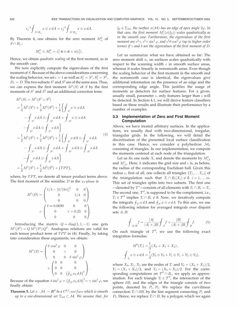
and simple way to determine the tangent basis ðw1;�; w2;�Þ.To illustrate this procedure, we show in Fig. 7 the

eigenvector w1;� corresponding to the largest eigenvalue of

the first moment as an arrow plot. The vector is shown only

in areas where the combined zero and first moment

classifier is larger than a given threshold, i.e., where

features such as edges and cusps are detected. Hence, w1;�

is aligned to the direction of the features (edges). As shown

by the detailed images in Fig. 7, the computation of the

feature directions is robust and reliable.Next, we define the application of the diffusion tensor

a�T �M to a vector z 2 R3 by

522 IEEE TRANSACTIONS ON VISUALIZATION AND COMPUTER GRAPHICS, VOL. 10, NO. 5, SEPTEMBER/OCTOBER 2004

Fig. 4. Zero moment (a) and combined (b) classifiers for the human

cortex in Fig. 3.

Fig. 5. Human cortex surface classified with zero moments (a) and

curvature classification (b).

Fig. 6. Classifier applied to different surfaces. Left column: C0� and right

column: C0;1� .

a�T �M z :¼ �T �M

�Gð0Þðz � w1;�Þw1;�

þ C0;1� ðz � w2;�Þw2;� þ ðz � nÞn:

ð6Þ

Here, �T �M denotes the orthogonal projection onto thetangent space T �M and we identify the operator on theabstract tangent space and the endomorphism in IR3.Furthermore, the function Gð�Þ is chosen as in Section 4.1,where, in our applications, ¼ 0:1 and � ¼ 20. Now, weapply a�T �M as diffusion tensor in the following type ofparabolic evolution problem:

Given an initial compact embedded manifold M0 in IR3,

we compute a one parameter family of manifolds

fMðtÞgt2IRþ0with corresponding coordinate mappings xðtÞ

which solves the system of anisotropic geometric evolution

equations:

@tx� divMðtÞða�T �M rMðtÞxÞ ¼ f on IRþ MðtÞ; ð7Þ

and satisfies the initial condition

Mð0Þ ¼ M0:

Hence, due to the anisotropy defined above, we enforce asignal enhancement in the direction of the eigenvectorcorresponding to the largest eigenvalue of the first moment.In the perpendicular direction on the tangent space, theamount of diffusion is determined by the combined zero andfirst moment classifier C0;1� , i.e., as a function of the surfacesmoothness. For f ¼ 0, we can rewrite the evolution problemby use of the notion of the generalized mean curvature ha�T �M(for the corresponding background, we refer to [3], [5]):

@tx ¼ �ha�T �Mnþ ðdivM a�T �MÞðxÞ:

Hence, the velocity @tx splits into a tangential componentand a component orthogonal to the surface,

�ðT �MÞ? @tx ¼ �ha�T �Mn;

�T �M @tx ¼ ðdivM a�T �MÞðxÞ:

Here, �ðT �MÞ? v ¼ ðv � nÞn (with n being the surface normal),

is the orthogonal projection onto the normal direction.The tangential part �TxM @tx causes a tangential drift of

the surface coordinates on the surface, but it does notinfluence the shape of the surface itself. Nevertheless, thisdrift property may result in degeneration of triangles in thecase of discrete surfaces. To avoid this problem, wereformulate (7) by

@tx� divM a�T �M;rMx�

� n�

n ¼ 0: ð8Þ

In the spatially discretized form, we project the displace-ment of the mesh nodes onto node normals. The nodenormals are recomputed after each mesh smoothing step.The problem is discretized by a semi-implicit time steppingscheme (cf. the algorithm by Dziuk [10] and its general-ization in [4]). Frequently, due to the robustness of ourclassification, it suffices to compute the classifier on theinitial noisy mesh once and use it subsequently for all thedeformation steps. The corresponding linear system issolved using CG-iterations. One deformation step takesabout two seconds on a mesh of 269,000 triangles on aPentium 4 PC at 1.7 GHz.

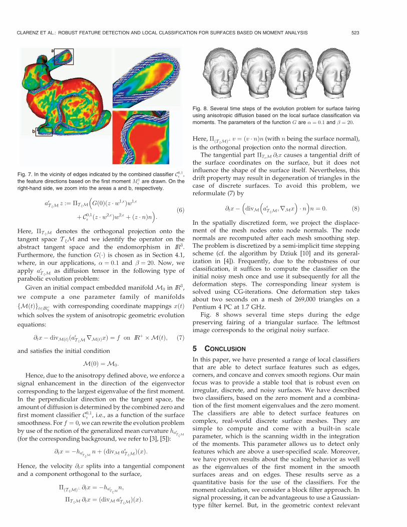
Fig. 8 shows several time steps during the edgepreserving fairing of a triangular surface. The leftmostimage corresponds to the original noisy surface.

5 CONCLUSION

In this paper, we have presented a range of local classifiersthat are able to detect surface features such as edges,corners, and concave and convex smooth regions. Our mainfocus was to provide a stable tool that is robust even onirregular, discrete, and noisy surfaces. We have describedtwo classifiers, based on the zero moment and a combina-tion of the first moment eigenvalues and the zero moment.The classifiers are able to detect surface features oncomplex, real-world discrete surface meshes. They aresimple to compute and come with a built-in scaleparameter, which is the scanning width in the integrationof the moments. This parameter allows us to detect onlyfeatures which are above a user-specified scale. Moreover,we have proven results about the scaling behavior as wellas the eigenvalues of the first moment in the smoothsurfaces areas and on edges. These results serve as aquantitative basis for the use of the classifiers. For themoment calculation, we consider a block filter approach. Insignal processing, it can be advantageous to use a Gaussian-type filter kernel. But, in the geometric context relevant

CLARENZ ET AL.: ROBUST FEATURE DETECTION AND LOCAL CLASSIFICATION FOR SURFACES BASED ON MOMENT ANALYSIS 523

Fig. 7. In the vicinity of edges indicated by the combined classifier C0;1� ,

the feature directions based on the first moment M1� are drawn. On the

right-hand side, we zoom into the areas a and b, respectively.

Fig. 8. Several time steps of the evolution problem for surface fairing

using anisotropic diffusion based on the local surface classification via

moments. The parameters of the function G are ¼ 0:1 and � ¼ 20.

here, this would require a corresponding time step of mean

curvature motion [4] as the geometric counterpart of

Gaussian filtering. Hence, we confine ourselves to the

simplest filter here, which, in particular, allows us to

present a detailed qualitative and quantitative analysis.Future work will address the use of the presented

surface classifiers, especially the combined one, for devising

better surface smoothing methods and for the multiscale

modeling of surfaces.

ACKNOWLEDGMENTS

The authors would like to thank Marc Tittgemeyer for

valuable hints on the cortex classification.

REFERENCES

[1] L. Alvarez, F. Guichard, P.L. Lions, and J.M. Morel, “Axioms andFundamental Equations of Image Processing,” ArchitecturalRational Mechanical Analysis, vol. 123, no. 3, pp. 199-257, 1993.

[2] V. Caselles, F. Catte, T. Coll, and F. Dibos, “A Geometric Model forActive Contours in Image Processing,” Numerical Math., vol. 66,1993.

[3] U. Clarenz, “Enclosure Theorems for Extremals of EllipticParametric Functionals,” Calculus Variations, vol. 15, pp. 313-324,2002.

[4] U. Clarenz, U. Diewald, and M. Rumpf, “Anisotropic Diffusion inSurface Processing,” Proc. Visualization 2000, B. Hamann, T. Ertl,and A. Varshney, eds., pp. 397-405, 2000.

[5] U. Clarenz, G. Dziuk, and M. Rumpf, “On Generalized MeanCurvature Flow,” Geometric Analysis and Nonlinear Partial Differ-ential Equations, H. Karcher and S. Hildebrandt, eds., Springer,2003.

[6] R. Deriche, “Using Canny’s Criteria to Derive a RecursivelyImplemented Optimal Edge Detector,” Int’l J. Computer Vision,vol. 1, pp. 167-187, 1987.

[7] M. Desbrun, M. Meyer, P. Schroeder, and A. Barr, “ImplicitFairing of Irregular Meshes Using Diffusion and Curvature Flow,”Computer Graphics (SIGGRAPH ’99 Proc.), pp. 317-324, 1999.

[8] M. Desbrun, M. Meyer, P. Schroeder, and A. Barr, “AnisotropicFeature Preserving Denoising of Height Fields and BivariateData,” Graphics Interface ’00 Proc., 2000.

[9] U. Diewald, S. Morigi, and M. Rumpf, “On Geometric Evolutionand Cascadic Multigrid in Subdivision,” Proc. Vision, Modeling andVisualization 2001, T. Ertl, B. Girod, G. Greiner, H. Niemann, andH.-P. Seidel, eds., pp. 67-75, 2001.

[10] G. Dziuk, “An Algorithm for Evolutionary Surfaces,” NumericalMath., vol. 58, pp. 603-611, 1991.

[11] C. Gotsman, S. Gumhold, and L. Kobbelt, “Simplification andCompression of 3D Models,” Tutorials on Multiresolution inGeometric Modeling, Springer, 2002.

[12] J. Jost, Riemannian Geometry and Geometric Analysis. Springer, 1998.[13] R. Kimmel, “Intrinsic Scale Space for Images On Surfaces: The

Geodesic Curvature Flow,” Graphical Models and Image Processing,vol. 59, no. 5, pp. 365-372, 1997.

[14] L. Kobbelt, S. Campagna, J. Vorsatz, and H.-P. Seidel, “InteractiveMulti-Resolution Modeling on Arbitrary Meshes,” ComputerGraphics (SIGGRAPH ’98 Proc.), pp. 105-114, 1998.

[15] F.F. Leymarie and B.B. Kimia, “Computation of the Shock Scaffoldfor Unorganized Point Clouds in 3D,” IEEE Proc. Conf. ComputerVision and Pattern Recognition, vol. 1, pp. 821-827, 2003.

[16] M. Meyer, M. Desbrun, P. Schroder, and A.H. Barr, “DiscreteDifferential-Geometry Operators for Triangulated 2-Manifolds,”Proc. VisMath Conf., 2002.

[17] H.P. Moreton and C.H. Sequin, “Functional Optimization for FairSurface Design,” SIGGRAPH ’92 Conf. Proc., pp. 167-176, 1992.

[18] S.J. Osher and J.A. Sethian, “Fronts Propagating with CurvatureDependent Speed: Algorithms Based on Hamilton-Jacobi For-mulations,” J. Computational Physics, vol. 79, pp. 12-49, 1988.

[19] P. Perona and J. Malik, “Scale Space and Edge Detection UsingAnisotropic Diffusion,” Proc. IEEE CS Workshop Computer Vision,1987.

[20] U. Pinkall and K. Polthier, “Computing Discrete Minimal Surfacesand Their Conjugates,” Experimental Math., vol. 2, no. 1, pp. 15-35,1993.

[21] T. Preußler and M. Rumpf, “A Level Set Method for AnisotropicGeometric Diffusion in 3D Image Processing,” SIAM J. AppliedMath., vol. 62, no. 5, pp. 1772-1793, 2002.

[22] M. Rumpf and A. Telea, “A Continuous Skeletonization MethodBased on Level Sets,” Proc. VisSym ’02, 2002.

[23] G. Taubin, “A Signal Processing Approach to Fair SurfaceDesign,” Computer Graphics (SIGGRAPH ’95 Proc.), pp. 351-358,1995.

[24] J. Weickert, “Foundations and Applications of Nonlinear Aniso-tropic Diffusion Filtering,” Z. Angew. Math. Mech., vol. 76, pp. 283-286, 1996.

[25] J. Weickert, Anisotropic Diffusion in Image Processing. Teubner,1998.

[26] J. Wu, S. Hu, C. Tai, and J. Sun, “An Effective Feature-PreservingMesh Simplification Scheme Based on Face Constriction,” PacificGraphics 2001 Proc., pp. 12-21, 2001.

Ulrich Clarenz studied mathematics at theUniversity of Bonn and received the Diploma in1996 and the PhD degree in 1999. In 2000 and2001, he worked for the Deutsche Boerse AG.Since 2001, he has held a postdoctoral researchposition at the University of Duisburg-Essen. Hisresearch interests are in analytical and numer-ical aspects of nonlinear partial differentialequations and the calculus of variations.

Martin Rumpf received the Diplom degree andthe PhD degree in mathematics from BonnUniversity in 1989 and 1992, respectively. Heheld a postdoctoral research position at FreiburgUniversity. Between 1996 and 2001, he was anassociate professor at Bonn University. Since2001, he has held the chair for NumericalMathematics and Scientific Computing at theUniversity Duisburg-Essen. His research inter-ests are in numerical methods for nonlinear

partial differential equations, geometric evolution problems, calculus ofvariations, adaptive finite element methods, image and surfaceprocessing.

Alexandru Telea graduated in 1996 in computerscience from the Polytechnics Institute of Bu-charest, Romania, and received the PhD degreein computer science in 2000 from the EindhovenUniversity of Technology (TU/e), The Nether-lands. Since then, he has been an assistantprofessor in visualization and computer graphicsin the Department of Mathematics and Compu-ter Science at TU/e. His research interests aremultiscale modeling and analysis for scientific

and information visualization, shape analysis and representation, andcomponent and object-oriented software architectures.

. For more information on this or any computing topic, please visitour Digital Library at www.computer.org/publications/dlib.

524 IEEE TRANSACTIONS ON VISUALIZATION AND COMPUTER GRAPHICS, VOL. 10, NO. 5, SEPTEMBER/OCTOBER 2004