University of Groningen

Considerations on modeling for early detection of abnormalities in locally autonomousdistributed systemsVeelen, Martijn van

IMPORTANT NOTE: You are advised to consult the publisher's version (publisher's PDF) if you wish to cite fromit. Please check the document version below.

Document VersionPublisher's PDF, also known as Version of record

Publication date:2007

Link to publication in University of Groningen/UMCG research database

Citation for published version (APA):Veelen, M. V. (2007). Considerations on modeling for early detection of abnormalities in locallyautonomous distributed systems. s.n.

CopyrightOther than for strictly personal use, it is not permitted to download or to forward/distribute the text or part of it without the consent of theauthor(s) and/or copyright holder(s), unless the work is under an open content license (like Creative Commons).

The publication may also be distributed here under the terms of Article 25fa of the Dutch Copyright Act, indicated by the “Taverne” license.More information can be found on the University of Groningen website: https://www.rug.nl/library/open-access/self-archiving-pure/taverne-amendment.

Take-down policyIf you believe that this document breaches copyright please contact us providing details, and we will remove access to the work immediatelyand investigate your claim.

Downloaded from the University of Groningen/UMCG research database (Pure): http://www.rug.nl/research/portal. For technical reasons thenumber of authors shown on this cover page is limited to 10 maximum.

Download date: 24-12-2021

Considerations on Modeling for Early Detection of Abnormalities

in Locally Autonomous Distributed Systems

Martijn van Veelen

RIJKSUNIVERSITEIT GRONINGEN

Considerations on Modeling for Early Detection of Abnormalities

in Locally Autonomous Distributed Systems

Proefschrift

ter verkrijging van het doctoraat in de Wiskunde en Natuurwetenschappen aan de Rijksuniversiteit Groningen

op gezag van de Rector Magnificus, dr. F. Zwarts, in het openbaar te verdedigen op

vrijdag 2 maart 2007 om 16:15 uur

door

Martijn van Veelen

geboren op 7 maart 1974

te Haarlem

Promotor: Prof. dr. ir. L. Spaanenburg

Copromotor: dr.ir. J.A.G. Nijhuis

Beoordelingcommissie: Prof. dr. P.W. AdriaansProf. dr. H. ButcherProf. dr. ir. C.H. Slump

IPA Dissertation Series 2007-03

ISBN: 90-367-2929-7 (hardcopy) ; 90-367-2930-0 (digital, pdf)

The work in this thesis has been carried out under the auspices of the research school IPA (Institute for Programming research and Algorithmics)

i

Table of Contents

Chapter 1 Introduction ....................................................................................................1

1.1 Automating beyond control.............................................................................. 11.1.1 The challenge ............................................................................................................11.1.2 The complexity of distributed systems .....................................................................21.1.3 The complexity of modeling .....................................................................................41.1.4 Deviations and disturbances......................................................................................51.1.5 The function of detection ..........................................................................................6

1.2 Detection approaches .......................................................................................61.2.1 The classical framework ...........................................................................................61.2.2 Strategies and techniques ..........................................................................................71.2.3 Principal challenges ..................................................................................................8

1.3 This research ....................................................................................................81.3.1 Research problem......................................................................................................81.3.2 Research objective ....................................................................................................91.3.3 Research questions ....................................................................................................91.3.4 Thesis ........................................................................................................................91.3.5 The role of neural networks ......................................................................................9

1.4 Thesis layout ..................................................................................................101.4.1 Outline.....................................................................................................................101.4.2 Pointers to related work discussed in this thesis .....................................................11

Chapter 2 Modeling & Estimation ................................................................................ 15

2.1 Sources: systems and processes .....................................................................152.1.1 Systems and processes ............................................................................................162.1.2 Information source ..................................................................................................162.1.3 Configuration, state space and manifestation..........................................................17

2.2 Data: observation and sampling .....................................................................192.2.1 Data sampling..........................................................................................................192.2.2 Data analysis ...........................................................................................................202.2.3 Preprocessing ..........................................................................................................22

2.3 Models: architecture and parameters..............................................................232.3.1 Objectives and definitions.......................................................................................232.3.2 Distribution estimation............................................................................................242.3.3 Function approximation and regression..................................................................252.3.4 Physically plausible models ....................................................................................262.3.5 Black-box models....................................................................................................282.3.6 Errors and disturbances ...........................................................................................28

2.4 Estimation: fitting, quality & limitations .......................................................302.4.1 Procedures for fitting data as a learning process.....................................................302.4.2 Risk, bias and variance............................................................................................332.4.3 Performance and error measures.............................................................................352.4.4 Control system theory .............................................................................................382.4.5 Complexity estimation ............................................................................................402.4.6 Fundamental limitations..........................................................................................422.4.7 Dealing with complexity through simplifications...................................................42

2.5 Summary ........................................................................................................43

Chapter 1

ii

Chapter 3 Neural Modeling ...........................................................................................45

3.1 Background ....................................................................................................453.1.1 Developments and evolution...................................................................................463.1.2 Neural networks overview ......................................................................................483.1.3 Applications for neural networks ............................................................................49

3.2 MLP-based dynamic models.......................................................................... 503.2.1 The Perceptron and alternative kernels ...................................................................503.2.2 The Multi-Layer Perceptron....................................................................................513.2.3 Dynamic extensions of the Multi-Layer Perceptron ...............................................523.2.4 Focused time-lagged architectures and gamma networks.......................................55

3.3 Neural estimation ...........................................................................................583.3.1 Procedures for fitting data.......................................................................................583.3.2 Error back-propagation ...........................................................................................593.3.3 Learning in dynamic neural networks.....................................................................623.3.4 Convergence and stopping criteria..........................................................................64

3.4 Neural design and learning issues ..................................................................653.4.1 Typical features of neural models ...........................................................................653.4.2 Observed neural design and learning problems ......................................................663.4.3 Problem analysis: typical features causing problems..............................................673.4.4 Neural design heuristics and architectural modifications .......................................713.4.5 Status-quo of neural design and learning issues .....................................................77

3.5 Summary ........................................................................................................78

Chapter 4 Detection for Controlled Systems................................................................79

4.1 Introduction ....................................................................................................794.1.1 Background .............................................................................................................794.1.2 Views on systems and abnormalities ......................................................................804.1.3 Process outline ........................................................................................................834.1.4 Requirements and criteria .......................................................................................854.1.5 Key functions and base techniques .........................................................................86

4.2 Statistical signal detection.............................................................................. 884.2.1 Preliminaries ...........................................................................................................884.2.2 Basic one-sample tests: residual analysis................................................................894.2.3 Basic two-sample tests for residual comparison.....................................................914.2.4 Dedicated filters ......................................................................................................934.2.5 Projection methods..................................................................................................944.2.6 Adaptive Filters.......................................................................................................954.2.7 Design, quality and optimality ................................................................................96

4.3 Fault detection and isolation .......................................................................... 974.3.1 Preliminaries ...........................................................................................................974.3.2 Dedicated filters ......................................................................................................974.3.3 Projection methods..................................................................................................984.3.4 State estimation through adaptive filtering ...........................................................1004.3.5 Blind Identification ...............................................................................................1024.3.6 Selecting an FDI strategy......................................................................................103

4.4 Computational intelligence .......................................................................... 1044.4.1 Preliminaries .........................................................................................................1044.4.2 Search and diagnostic methods .............................................................................1054.4.3 Applications of neural networks in detection........................................................107

4.5 Discussion ....................................................................................................1084.5.1 Overview of the techniques organized by underlying mechanisms......................1094.5.2 Problem domain ....................................................................................................109

4.6 Summary ......................................................................................................111

iii

Chapter 5 Problem Analysis ........................................................................................115

5.1 Applications in distributed systems..............................................................1155.2 Inspiring phenomena....................................................................................118

5.2.1 Industrial plant: a hot strip mill .............................................................................1195.2.2 Network services: communication........................................................................1215.2.3 Sensory networks: low frequency array................................................................1235.2.4 A refinement of the problem domain ....................................................................126

5.3 Analysis of possible causes.......................................................................... 1285.3.1 Control strategies are inadequate ..........................................................................1285.3.2 Disturbances: global disturbances.........................................................................1295.3.3 The complexity of modeling .................................................................................1315.3.4 Pitfalls of conventional approaches ......................................................................136

5.4 Problem statement ........................................................................................1385.5 Conclusions ..................................................................................................139

Chapter 6 Early Abnormality Detection .................................................................... 141

6.1 Motivation and preliminaries .......................................................................1416.1.1 A view on systems and abnormalities...................................................................1416.1.2 The problem of modeling limitations in detection................................................1446.1.3 Causes and consequences of bias..........................................................................1466.1.4 Purpose and organization of this chapter ..............................................................148

6.2 Why redundancy inside the model? .............................................................1496.2.1 The driver of observability....................................................................................1496.2.2 Channel analogy....................................................................................................1496.2.3 Observability versus reductionism........................................................................1516.2.4 Reasons to avoid assumptions on system and abnormalities ................................1546.2.5 Arguments for redundant modeling ......................................................................154

6.3 Separate long term analysis from early detection........................................1566.3.1 Earliness ................................................................................................................1566.3.2 Array processing inspiration .................................................................................1576.3.3 Blind identification versus earliness .....................................................................1586.3.4 Separate long term analysis from early detection .................................................160

6.4 What to detect, and why monolithic modeling?...........................................1606.4.1 Focus on amount of structure in drift ....................................................................1606.4.2 Monolithic modeling.............................................................................................162

6.5 Redundancy, complexity and risk ................................................................1646.5.1 Redundancy versus minimal-risk..........................................................................1646.5.2 Risk-invariant redundancy ....................................................................................1666.5.3 A soft-scaling complexity .....................................................................................167

6.6 Conclusions ..................................................................................................169

Chapter 7 Intermezzo - Towards a detection method ...............................................173

7.1 Detection strategy.........................................................................................1737.1.1 Design objectives and the key mechanisms..........................................................1737.1.2 Overall detection strategy clarifying the role of models and data ........................1747.1.3 Verification and optimization of design................................................................176

7.2 Design considerations for the neural process model....................................1777.3 Positioning the detection procedure .............................................................178

Chapter 1

iv

Chapter 8 Neural Abnormality Detection ..................................................................181

8.1 Feasibility of modeling for early detection ..................................................1818.1.1 Data-driven dynamic modeling.............................................................................1818.1.2 Soft-scaling complexity ........................................................................................1838.1.3 Common features from multiple instances ...........................................................1878.1.4 Meeting modeling requirements for early detection .............................................188

8.2 Signature computation..................................................................................1888.2.1 Survey of neural metrics .......................................................................................1898.2.2 Selection of metrics...............................................................................................190

8.3 Computer experiments .................................................................................1938.3.1 Illustration of the design with a sine-wave prediction example............................1938.3.2 Robust non-deterministic detection for a Volterra-Lotka system.........................1958.3.3 Design consideriations ..........................................................................................198

8.4 Related work on early detection...................................................................2008.4.1 Detection based on a quantitative modeling .........................................................2008.4.2 Detection based on process history information...................................................200

8.5 Conclusions .................................................................................................204

Chapter 9 Concluding Remarks..................................................................................205

9.1 Contribution of this research........................................................................ 2059.2 Recommendations ........................................................................................208

9.2.1 Applications ..........................................................................................................2089.2.2 Future research ......................................................................................................209

9.3 Conclusions ..................................................................................................210

Postscript: Emergent behavior ........................................................................................ 215

Emergent behavior ...................................................................................... 215Links of this thesis to emerging behavior ................................................... 215An exemplary formulation of emergent behavior ....................................... 216Modeling requirements for discovery of emergent behavior ...................... 220A final insight.............................................................................................. 220

Appendix A Math and notations.......................................................................................... i

A.1 Typesettings math objects ................................................................................. iA.2 Descriptive statistics and probability ................................................................ iA.3 Information theory............................................................................................iiA.4 Signal processing..............................................................................................iiA.5 Artificial Neural Networks............................................................................... ii

Appendix B Solving and Linearizing ...............................................................................iii

B.1 Solving ............................................................................................................iiiB.2 Linearization..................................................................................................... vB.3 Deriving the Extended Kalman Filter equations.............................................. v

Appendix C List of Abbreviations ..................................................................................... ix

Appendix D Statistics and Signal Detection......................................................................xi

v

D.1 Statistical properties ........................................................................................xiD.2 Information Theory ........................................................................................xiiD.3 Signal detection theory..................................................................................xivD.4 Capon’s regularity conditions ........................................................................ xvD.5 Applications of Hankel matrices....................................................................xv

Appendix E List of neural metrics ..................................................................................xix

Chapter F Pruning Example .........................................................................................xxi

F.1 Simulated data ...............................................................................................xxiF.2 Pruning results..............................................................................................xxii

Appendix G Biography ...................................................................................................xxiii

G.1 About the author..........................................................................................xxiiiG.2 List of publications......................................................................................xxiii

G.2.1 This research ....................................................................................................... xxiiiG.2.2 Embedded systems research................................................................................ xxivG.2.3 Radiotelescope system design research .............................................................. xxivG.2.4 Speech recognition and digital signal processing .................................................xxv

G.3 List of public presentations .......................................................................... xxv

Appendix H Titles in the IPA Dissertation Series since 2002.....................................xxvii

Bibliography ..................................................................................................................... xxxi

Samenvatting .................................................................................................................... xlvii

Dankwoord............................................................................................................................. li

Chapter 1

vi

Automating beyond control Chapter 1 INTRODUCTION

1

Chapter 1

Introduction

The automation and evolution of networked applications brought locallyautonomous distributed systems with global quality attributes. These systemshave moved beyond acceptable manageability. Both design and applicationare unavoidably imperfect due to the complexity of modeling and conse-quently systematic errors appear. The classical detection approaches arelimited in their coverage. Hence, to advance the state of the art, a betterunderstanding is needed of the requirements for early abnormality detectionin locally autonomous distributed systems with global functions.

In this chapter we introduce the motivation and background concepts required for the discus-sion of early detection of abnormalities in locally autonomous distributed systems. The needfor detection occurs when a system does not fit well in it’s embedding environment. This maybe because the environment was not fully understood when the system was designed orbecause it has simply changed since then. Things can get out of hand when the system reactsaccording to a wrong perception of the world around it. Detection is then brought into play toavoid such misbehavior. In section 1.1 we discuss the application domain of Locally Autono-mous Distributed Systems (LADS) with global quality attributes, which raises the issue ofmodeling and detection. The classical detection framework, classical methods and techniques,are introduced in section 1.2. Finally, in section 1.3 the objective, the problem and the relatedresearch questions addressed in this thesis are explicitly stated.

1.1 Automating beyond control

1.1.1 The challenge

We have become highly dependent on very complex man-made distributed systems for energyproduction and transport, communication, environmental monitoring and industrial produc-tion. These increasingly automated systems are growing beyond manageability. Many strate-gies and techniques, though well-founded on physics and mathematics, do not provide asystem design that is correct-by-construction. To make imperfection acceptable, the involvedrisks in terms of cost and potential harm to others demand at least an adequate approach to pre-vent the worst to the largest affordable extent. Methods well-founded on physics and mathe-matics often fail to provide an adequate approach to accommodate a priori unknown but actualimperfections, which is why computational intelligence is called upon. The alarming observa-tion is made that the well-founded arsenal, including rigorous exact modeling, fails to bringsufficient manageability and sufficiently predictable behavior of the increasing complex man-made systems that have become the fabric of our society. This poses the challenge that we takeup in the coming discourse.

INTRODUCTION Chapter 1 Automating beyond control

2

1.1.2 The complexity of distributed systems

Welfare has increased in the previous century through the expansion of Signal, Electricity,Water and Natural Gas Grids. A recent addition is the Information Grid (or Internet). This doesnot only enrich the classical networks, but also stimulates new sensory ones in Home andIndustry [Amin, 2002]. The default distribution of a programming error as part of the mainte-nance procedure, that in 1992 causes the New-Jersey blackout, may have seemed just anexception at that time. But the problems keep coming back. Foremost the Allston-Keeler (July1996) and the Galaxy-IV (May 1998) disasters gave rise to a concerted research activity onSelf-Healing Networks [Amin, 2000]. In general the probable cause is a lack of investment toensure proper operational conditions as a result of commercializing national and global respon-sibilities. The series of three disasters on the Electricity Grid in Autumn 2003 (in respectivelyAmerica, Sweden and Italy) suggests that little progress has been made. And this is only the tipof an iceberg [Amin, 2003; Barabasi 2003].

Predictable behavior is key to prevent malfunction. In energy Grids, the EC recently called forEU wide governance. It is already a national concern, and for good reasons. These networksgrow without an overall architectural vision but rather by means of a local preferential attach-ment. Despite the lack of predetermined structure a seemingly chaotic self-organization leadsto a structure, though often surprisingly different from the topology of designed networks[Barabasi, 2003]. Automation brought LADS, which displays seemingly unpredictable behav-ior. What led to this situation?

Figure 1.1 : Jacquard pattern looms in the factory Gevers & Schmidt in Schmiedeberg (Silesia). Thepattern is entered via punched cards. (Wood engraving from 1858, · Deutsches Museum, München)

Expansion of man-made systems and industrial automation is an interaction of market-pull andtechnology-push. Industrial automation has a long history starting with the advent of machinesdriven by windmills in the Dutch Zaanstreek in the 17th century, over automation in the spin-ning and pattern weaving industry (figure 1.1) via the production streets popularized by Fordin the early 20th century to semi-automatically managed energy production and distributionsystems. In automated processing the pursued short time-to-market and technology adaptive-

Automating beyond control Chapter 1 INTRODUCTION

3

ness induces rapid replication of errors: "in ultra-dependable systems even a small correlationin failures of the replicated units can have a significant impact on the overall dependability"[Bouyssounouse & Sifakis, 2005]. The accumulation of such deviations into an harmful failuremust be prevented by a pro-active rather than a reactive attitude.

The network concept has moved in various directions. Sensory1 networks have become preva-lent in Home and Industrial Automation. They display a high degree of heterogeneity, whichadds to the system complexity and therefore implies reliability problems [Bullinger, 2004]. Inthe evolution of ever more complex and more automated systems, the risks in terms of damageand cost increase. These risks are unacceptable when a potential disaster is at hand, no matterwhat the probability is. Risks are highly inconvenient when they touch upon our well-being,such as by a loss of electric power, communication or public transport. They are merely unde-sirable and costly when the performance and availability of a system or instrument do not meettargets. In the economy of industry and governmental responsibility, investments follow risk-management strategies. The quality of a product or service is expressed in probabilities; imper-fection is a design criterion, dictated by return-on-investment. The prevaling risk-managementstrategies optimize but not minimize the failure probability.

We have a responsibility for the man-made technological systems exploiting natural principlesand resources. Such is in the hands of those who can perceive the patterns, rather than theunaware actors within the system. Responsibilities, besides those economically motivated,concern prevention, precaution and at least minimization of potential harm by guarding andguiding the environment. "A grand challenge for science is to understand the human implica-tions of global environment change and to help society cope with those changes. Virtually allthe scientific questions depend on geospatial information. Another challenge is to respond tocalamities, terrorist activities, other human-induced crises, and natural disasters. Much of thework addressing environmental- and emergency-related concerns will depend on how produc-tively humans are to integrate, distill, and correlate a wide range of seemingly unrelated infor-mation" [National Research Council, 2003]. Next to the responsibility for man-made systemsthere is an increasing demand to monitor ecosystems both for economic and safety purposes.Geospatial sensory networks can offer early warning for earthquakes on land or in the oceanthat may cause tsunamis. However early detection depends on detecting and localizing patternswithout exact, physically plausible models. The resolution and coverage of sensor networksare rapidly increasing, causing an overwhelming stream of data. The intelligence of humaninterpreters needs to migrate into automated systems.

Complex distributed systems become monoliths through attachment. Systems that are initiallyisolated become super-systems when distinct inseparable global functions and qualities arepursued. Other systems are intentionally designed for global functions and qualities, e.g. thenew generation of radio-telescopes LOFAR and SKA. Global functions are eminent, while dis-tinct sub-functions are no longer isolated in sub-systems; these types of systems are really dif-ferent from classical FDI (Fault Detection and Isolation) applications like airplanes, andisolated chemical systems and power plants. Distributed systems with global functions differ

1. The word sensor network refers to the system or platform, it is a network with sensors. The word sen-sory or sensing network is used for applications which pursue to benefit from the combination of sen-sor signal. In the sensory network concept a central model of an observed entity is calibrated using the sensor data. Sensory networks are sensor networks, but a sensor network is not necessarily a sensory network. We have used the concepts indiscriminately, their meaning will be clear from the context.

INTRODUCTION Chapter 1 Automating beyond control

4

from robots, where the vision and the arm-movement are different sub-systems with a distinctfunction. This has major implications for the quality management, since it is no longer clearhow the quality of sub-processes contributes to the quality of the end-product; it is hard to ana-lyze global quality aspects as the disturbance propagation is very complicated.

Distributed systems with global functions demand a coherent co-operation. Control mecha-nisms are an integral part in most dynamic systems, guiding them towards desired behavior.Control is designed purposefully into systems. In ecosystems the dynamics result from facilita-tion and competition over resources. Where craftsmanship turns into automation usingmachinery, human-guided processes and machines further evolve to connected distributed sys-tems. In the expansion appears an increasing effort to steer the interaction of components, ashuman-operations are replaced by hierarchical PID-control. Increased organizational complex-ity and accurately timed closed-loop control appear in local processes. Consequently globaldirect control over all components is in many instances no longer possible, resulting in autono-mous subsystems. Local autonomous processing and the hierarchical distribution of set-pointsallow for this. In a new generation of distributed systems, self-organization appears. Who man-ages the consequences of these developments on the requirements for health monitoring?

1.1.3 The complexity of modeling

There is mathematics (a truth but only within itself), there is statistics, and there is artificialintelligence. These three areas have struggled and competed in an ongoing effort to describethe world as we see it with the ultimate goal of control through technological advances. Eversince the industrial revolution we have become increasingly dependent on technology. It isinevitable that we slowly have recognized the limitations of our understanding of the processesin an effort to describe and control. Many processes are not well understood and confront uswith unforeseen events and unexplained behavior, often to our detriment. We observe, sampleand store huge amounts of measurements, but conventional models and modeling techniquesfail to increase our understanding in the complex behavior of the underlying processes.

A system design starts from a conceptual, desired function. The expertise to construct a modelmay have been assembled over a long time and formulated into generally valid natural laws,such as Ohm's Law or Maxwell's equations. Engineering always puts a strong emphasis on theability to formulate the exact model for design purposes. Such a model can be used as a frameof reference. Future developments will have the model as common starting point, describing acommon understanding for all concerned. The model derived from first principles is oftenassumed to suffice for design and control purposes.

A case of modeling complexity: designing the new generation of radio-telescopes

The Dutch low-frequency array (LOFAR) is a new type of telescope for conducting radioas-tronomy at low frequencies, with large instantaneous bandwidth (32MHz) and unpreceded sen-sitiviy and resolution and multi-beaming capability. The LOFARs infrastructure is also utilzedfor several sensor network applications. The essense of LOFAR is a coherent acquisition andprocessing of data to fit accurate dynamic models of natural phenomena approximately in real-time. We have conducted the feasibility and preliminary design studies for the LOFAR sta-tions, and as such participated in the system group. The LOFAR design objectives are a typicalchallenge to squeeze the most out of emerging technology capabilities to provide, within a lim-ited budget, a highly competitive and unique multi-purpose facility to a demanding and critical

Automating beyond control Chapter 1 INTRODUCTION

5

customer. All the digital subsystem design issues are highly intertwined with the design andissues of analog/RF front-end and the backend signal transport and central processing. The useof a global system model that leaves the necessary room for options to be offered by emergingtechnologies is used in the subsystem design. The lack of a very detailed system design is athreat to the convergence of (a) the system design studies and requirements, and (b) the systemspecification discussions. We have a collective learning process where unknown subsystemproperties need to be integrated successfully into a large system. A detailed end-to-end simula-tion, to that purpose, has been advocated but was never achieved. These experiences show thatan adequate system model is already beyond reach in design, despite a competent and focusedteam effort.

The difficulties in modeling locally autonomous distributed systems

The difficulties in modeling arise from the complexity of system behavior: dependenciesappear where they are not expected and variability occurs instead of consistent and predictablebehavior. Either way time-variant behavior is a rule rather than exception, and abnormalitieshave to be identified from volatile measurements. The essential difficulties that are generallyagreed upon, are: hidden dependencies [EEUMA, 1999]; variability [Venkatasubramanian,2003]; and, interaction of a system with an unknown environment [Lisboa, 2001].

A common remedy: divide and conquer

A fine-grain exact model for design and control implementation is too complex for large sys-tems; therefore feasibility (both of the design as well as in the control) depends on a divide-and-conquer approach. A system is composed hierarchically out of subsystems, subsystemsout of sub subsystems, etc. down to a level of detail where desired function, form and resultingbehavior coincide. This is the level of logical or physical components. On this level of abstrac-tion, where desired function, form and behavior coincide, a model is derived straightforwardlyfrom logical or physical principles.

1.1.4 Deviations and disturbances

Deviations are differences between the behavior that can be explained from the model and theactual system. A model is as good as the supporting measurements. Consequently reality maybe different from the design concept and disturbances may occur, as: 1) measurements areinfluenced by other than the intended subset of measurements; 2) models are incomplete, i.e.they do not describe the process or entity as it is, and 3) measured processes and entities aresubject to change. Usually these effects are present simultaneously and cannot be easily iso-lated in their net effect. Though the different ingredients of disturbances are modeled withvarying levels of detail, it is generally agreed upon that two types of disturbances can be distin-guished: unstructured and structural errors. Random errors cannot be prevented, as they areunstructured by definition. There is no meaningful extension or alteration to the existing modelto reduce such problems. Unstructuredness can result from numerical imprecision, chaos andinseparability of a single data source out of the many influencing the measurements.

The model should remain a good representation of the data source, hence it must accommodatesystematic errors. Therefore we need to recognize the conditions, under which the model canbe improved. If there is a source of disturbances in profound interaction with the data source, itwill cause structural dynamic disturbances that evolve towards unacceptable performance deg-radation. Revealing the presence of such sources is the goal of this research.

INTRODUCTION Chapter 1 Detection approaches

6

1.1.5 The function of detection

The purpose of fault detection, diagnosis and accommodation in real-world applications are: 1)to increase availability of the production process; 2) to enhance efficiency of the productionprocess; 3) to improve safety of the process; 4) to increment quality of the end-product or pro-vided service. Detection is a function complementary to the systems nominal operation, aimingat accommodation of deviations which are not treated by the systems control. Detection of dis-turbances facilitates the identification of wear, damage and other changes in the process.

1.2 Detection approaches

1.2.1 The classical framework

Detection is decision making or rather hypothesis testing based on a residual error signal. Thefollowing steps are generally agreed upon to make a decision:

1. model: to represent the known and expected behavior;2. sign: to compute an efficient representation of the residual;3. compare: to compare signatures of different measurements of presumed behavior;4. decide: to use information from the comparison(s) establishing the factual discrepancy.

Figure 1.2 : Isermann’s framework for detection and diagnosis [Isermann, 1984]

The, by now paradigmatic, framework for detection is shown in figure 1.2. At it’s heart is thephysical-principle model, which through state and parameter estimation allows for a transfor-

N

eventtime

faul

t det

ectio

ndi

agno

sistype

locationsizecause{

theoretical process model

normal process

faulty process

fault

fault {

uy

θ

p

0p

pp σµ ˆ,ˆ

1p

data

pr

oces

sing

feat

ure

extr

actio

n

parameter estimation

calculation of process coefficients

determination of changes

fault decision

fault classification

process

Detection approaches Chapter 1 INTRODUCTION

7

mation of measurements to physical properties or so-called non-directly measurable quantities(NMQ). These physical properties are interpreted and classified and yield a diagnosis includ-ing the location and cause of fault in case it is present.

1.2.2 Strategies and techniques

Two partitions divide diagnostic methods into four categories. The first partition separates pro-cess-oriented (white-box) approaches from process history based (data-driven) approaches.The second partition separates qualitative methods from quantitative models. Detection anddiagnosis techniques are classified [Venkatsubraminian, 2003] into these categories. The qual-itative techniques are: 1) causal models and abstraction hierarchy; and 2) expert systems andquantitative trend analysis. These approaches are not considered in this research. We considerapproaches that rely on both a model as well as measurements. These approaches are dividedthree ways: 1) residual vs. parameter-based (figure 4.4); 2) data-driven vs. process-oriented; 3)self-organized vs. supervised estimation; (figure 4.3 illustrates the latter two classifications).

Residual-based vs. parameter-based

In a residual-based approach, the error of the model is directly used to compute signatures. Inparameter-based methods the parameters of a model serve to compute the signatures. Estima-tion is essential in parameter-based signature computation. In case the model is a priori incom-plete, on-line observations are required to calibrate the model to keep it up-to-date.

Process-oriented or white-box modeling.

A key assumption that underlies the classical detection approach is: Given an optimally con-trolled system the residual can be assumed to be stationary. If not, there is an abnormality.Given the state-space equations, derived from quantitative physics, the system designer canreach optimal control by forcing equilibrium in state space. Quantitative techniques that willbe considered in chapter 4 are: dedicated observers, parity spaces and Kalman filters.

Data-driven and black-box modeling

A contemporary problem in both process control and identification as well as in data-mining isthat in many situations there is no clear notion of an underlying process which can be modeledby a physically plausible process model while there is a huge amount of data. In contrast to amodel-based approach, computational intelligence is founded on data-driven approaches. Theyallow for descriptive model construction in the absence of physically plausible process models.

Self-organizing vs. supervised fitting

Parameter-based methods fit measurements pursuing a specific functional relationship. This isreflected in the coding problem (input-target) and the model architecture. This form of estima-tion is called supervised. The process-oriented parameter-based approach is supervised. Black-box models can be supervised as well as self-organized. Unsupervised estimation is an unre-stricted adaptive projection of data. They are founded on PCA (principal component analysis)pursuing a best linear separation between signal and noise space. It allows for a blind analysisof any dynamic and static dependencies between possibly hidden features. Kohonen maps andART (adaptive reasonoance theory) are examples of self-organizing neural models.

INTRODUCTION Chapter 1 This research

8

1.2.3 Principal challenges

Key detection and diagnosis performance criteria are [Venkatasubramanian, 2003]: sensitivity;promptness; isolatability; robustness; novelty identifiability; a quantified figure of merit;adaptability, explanation facility; modeling requirements; storage and computational require-ments and multiple fault identifiability.

Fundamental trade-offs in the criteria are [Isermann, 1984]: the size-of-fault vs. the requireddetection-time, the speed of fault vs. process response time, the speed of fault vs. detectiontime, the size and speed of faults vs. maximal speed of process parameter changes and thedetection time vs. false alarm rate. The crucial trade-off is promptness vs. robustness: the sta-tionary window vs. analysis or detection window. Or, to put it differently, the number of mea-surements for establishing the abnormality needs to be sufficient to fit a model confirming it’spresence with sufficient confidence.

There is a key trade-off between robustness to various noise contributions & uncertainties, andisolatability. Under ideal conditions, having freedom from noise and and modeling uncertain-ties, the detector should project measurements onto a space where output response is orthogo-nal to faults that have not occurred. To obtain a signal trend that is not too susceptible tomomentary variations due to noise, some kind of filtering needs to be employed. Filters sufferfrom the fact that they cannot distinguish well between a transient and a true instability [Ven-katasubramanian, 2003]. Systems designed to respond quickly to certain abrupt changes mustbe sensitive to high-frequency effects, hence they are more sensitivity to noise. [Wilsky, 1976].

There is a trade-off between sensitivity and promptness vs. novelty identifiability. One hasaccess to a good dynamic model but it is possible that much of the abnormal operations regionmay not have been modeled adequately. The timely reaction of a detection algorithm may beimpaired by the desire to handle various kinds of a priori unknown abnormalities (Universal-ity). Conventional process-oriented FDI relies on a comparison of reality with a pre-developedmodel of the ideal process to facilitate a swift decision-making. Supervised learning raises thesensitivity by modeling a range of faults on the basis of "golden" (desired and ideal) behavior,while a level of self-organization suffices for monitoring. A trade-off to optimize for an appro-priate choice of design parameters determines the success of any detection approach.

1.3 This researchThis research focuses on an intersection of the detection challenges in relation to properties ofLADS (locally autonomous distributed systems) with global functions. We offer a new per-spective, in the scope set by this intersection, positioning several new ideas in a coherent anal-ysis. This dissertation provides new understanding that is supported by a synthesis ofrequirements from an analysis of the limitations of the existing "classical" arsenal.

1.3.1 Research problem

Our problem is to detect early, to identify a change before it becomes a fault or a failure. Thisproblem is the detection of systematic deviations before they result in undesirable states inLADS within the global function and quality objectives.

This research Chapter 1 INTRODUCTION

9

1.3.2 Research objective

Our objective is improved understanding of design aspects of a detection procedure: identifica-tion of the properties of the detection problem (properties of system and abnormalities), lead-ing to selection of a detection strategy and techniques, and an evaluation of potential(dis)advantages for required innovation.

1.3.3 Research questions

The key question of this research is: “Is a disturbance the result of a system that changestoward an undesirable state or of an incomplete model?”. We seek an answer by investigating:

1. If it is possibility to identify the presence of a priori unknown potentially harmful struc-ture from time-variant behavior?

2. What are the limitations of the existing arsenal of strategies and techniques?3. What causes the limitations of the existing strategies and techniques? How do they relate

to properties of the detection problem (features of system and abnormalities)?4. Can neural networks offer a solution by modeling the dynamics in the data utilizing their

on-line learning capabilities.

1.3.4 Thesis

Despite the physical and mathematical foundation of the disciplines involved in system designand operation, the pragmatic industrial R&D sections have opened up to less conventionaltechniques, i.e. computational intelligence, to complement the existing arsenal. Computationalintelligence includes quantitative methods such as neural networks, fuzzy logic and evolution-ary algorithms. Our research originates from this setting, i.e. to investigate the potential meritsof neural networks to detect and reduce time-related disturbances in batch-oriented processes.

Modeling real-world systems while pursuing physical plausibility has scarcely increased theunderstanding for coping with the unexpected. Our quest is to identify unexpected patternsdirectly from behavior, instead of through after-the-fact analysis of a physically plausiblemodel. We consider whether neural networks are usable for this purpose.

1.3.5 The role of neural networks

Detection based on physical principle models pursues accurate diagnosis by exploiting a strongrelation between the topology of the source and the architecture of a detection model. As fine-grain modeling from the physical principle models is neither effective nor strictly necessary fordesign purposes the accurate model is often not available for operational system monitoring.Nonetheless huge amounts of monitoring data needs to be inspected for early detection andfailure prevention. Computational intelligence provides models to identify patterns in data. Wehave chosen multi-layer Perceptrons since these neural networks can serve as process modelsof dynamical systems which is not obvious for other models. Moreover their supervised gradi-ent-based adaptation allows for a preferred parameter based detection.

This thesis considers the features of neural network black-box modeling for detecting abnor-malities in complex and large data sets, seeking an effective comparison of data in the absenceof a physically plausible model. We focus on neural networks because of three particular fea-tures: self-organizing internal behavior; associated continuously and iterative adaption proced-cures; and the ability to the approximate continuous functions. They offer a middle way

INTRODUCTION Chapter 1 Thesis layout

10

between gross simplifications and complexity explosion by providing a model to inspectdependencies at an effective and efficient level of detail. Redundancy is often used for recogni-tion purposes. Recognition is improved by comparing multiple independent representations ofthe same entity. Nature provides inspiring examples of this mechanism. We will exploit thebenefits of redundancy inside the neural model.

1.4 Thesis layout

1.4.1 Outline

This thesis contains two parts. Part I is primarily a classification of the prior art coveringdynamical modeling of systems and disturbances, and detection theory. It includes a basicunderstanding of modeling and estimation of systems and signals (chapter 2); dynamical neu-ral networks (chapter 3); understanding neural design and neural learning (chapter 3), andunderstanding the arsenal of detection strategies and techniques (chapter 4). Part I equips uswith a solid background on modeling for detection, both physical principle and statisticalapproaches as well as at least one example of an alternative to mathematically foundedapproaches: neural networks that detach the modeling from any assumed physical or logicallaws. Part II covers a new perspective on the required modeling for early detection and an anal-ysis of the problems and synthesis of requirements. Part II consists of an problem analysisinspired from real-world phenomena (chapter 5); a synthesis of the essential requirements andkey design trade-offs (chapter 6); and an exploration of a neural solution (chapter 7 and 8).

Chapter 2 introduces the basics of modeling and estimation of signals and systems. We assumefamiliarity with such basic techniques and issues in part II of the thesis. It discusses the tech-niques for data analysis and problem coding, the basic issues concerning model complexity,and fundamental limitations such as solvability and observability.

Firstly, chapter 3 introduces neural modeling to capture dynamics in data and new patterns insystems and data. The principle mechanisms are time-series modeling and accommodation.We provide a classification of dynamic neural networks [vanVeelen, 2000a] and an evaluationof neural temporal PCA [vanVeelen, 1999]. Secondly, chapter 3 introduces neural network fea-tures that clearly distinguish them from classical modeling approaches, i.e. physical principleand statistical modeling. Chapter 3 also addresses neural design issues, relating symptoms toneural features, linking it to remedies and applied neural metrics. These neural metrics reap-pear in chapter 8 when we consider neural modeling and signature computation from neurallearning behavior for early detection.

Chapter 4 provides a survey of methods and techniques found in signal detection and FDI,resulting in a classification of methods that relate the properties of abnormalities and systems.We discuss reasons to apply computational intelligence in detection including possible scenar-ios to apply learning for detection [van Veelen 2000b].

Chapter 5 is an analysis inspired from an exploration of the phenomena in the design and useof LADS. We discuss the causes of limitations of the classical detection arsenal [van Veelen,2004, 2005]. A key contribution is the increased understanding of the gap between the natureof abnormalities occurring in practice and the capabilities of classical detection approaches.

Chapter 6 provides the motivation for the set of essential modeling requirements to address theearly detection problem, synthesized from the identified limitations and their causes.

Thesis layout Chapter 1 INTRODUCTION

11

The procedures discussed in the intermezzo (chapter 7) are not a part of the thesis theory(which is on the modeling requirements rather than on a specific detection procedure). Thetechniques and procedures in chapter 7 are given without further proof. In chapter 8 we arguethe potential of neural modeling and estimation to meet the modeling requirements. It dis-cusses neural features in relation to the derived requirements, we illustrate the required neuralcapability [van Veelen, 2000c, vanderSteen 2001] in addition to some recent publications inour problem domain.

1.4.2 Pointers to related work discussed in this thesis

We have not discussed the related work for the topics of this thesis in isolation since the relatedwork is quite extensive and diverse. Instead we provide a few pointers here to the related workdiscussions found in various contexts throughout the thesis. A discussion of work by others onthe investigated techniques and methods is found in:

• Section 2.2.2 discusses methods for time series analysis.

• Section 2.3 provides a short overview of various methods to model systems and data.

• Section 3.4.4 provides a survey of metrics for the analysis of learning in neural networks.

• Chapter 4 is a literature survey of conventional methods for detection.

The discussion on work by others comparable or directly related to this research is found in:

• Section 4.4.3 provides an overview on the use of neural networks in a conventionaldetection approach, i.e. the neural network does not replace the conventional systemmodels.

• Section 5.2 includes references to published application specific research for the cases.

• In section 7.4 we discuss those methods that also seek alternatives to overcome limita-tions of the conventional approaches, either using a similar model or using a similarapproach for detection or diagnosis.

Furthermore comprehensive discussions on work of others related to the various topics in thisthesis can be found in the published papers, listed in appendix G..2.1, related to this research.

INTRODUCTION Chapter 1 Thesis layout

12

PART I

ORIENTATION

'Let me put it this way, Mr. Amer. The 9000 series is the mostreliable computer ever made. No 9000 computer has ever madea mistake or distorted information. We are all, by any practicaldefinition of the words, foolproof and incapable of error.'

- HAL, from "2001, A Space Odyssey”

0, <Year>

Sources: systems and processes Chapter 2 MODELING & ESTIMATION

15

Chapter 2

Modeling & Estimation

Designing and operating machinery such as industrial plants requiresunderstanding of the relevant physical principles. Automatic control is anessential ingredient that depends on understanding to translate desired resultto necessary actions. This essential understanding is reflected in a model,also called a blue-print. Formal methods to model complex systems, startingbottom-up from the principles at the finest level of physical detail, have diffi-culty to provide coherent models of global behavior, especially when non-lin-ear processes are involved. Consequently, for adequate operation, it is oftennecessary to update a model using measurements, resorting either to on-linefeedback control and/or online re-estimation of the control model. We intro-duce the models for control and fitting of data, and consider the fundamentallimitations of modeling, control and estimation. Both formal hypothesis-driven methods as well as data-driven methods yield imperfect models. Time-series analysis and dynamic modeling can reveal structure in time, asrequired to detect disturbances resulting from imperfections. This chapteralso introduces principles of time-series analysis and dynamical modeling.

This chapter introduces elementary ways to construct a model, and to fit or identify a modelfrom data, either based from a blueprint or from behavior only. A discussion on modelingought to start with a perspective on systems and processes; particularly the statistical and phys-ical view, section 2.1 gets us started. We consider in section 2.2 how data is observed, sampled,ordered in a database and how it is prepared for modeling using data analysis and preprocess-ing. We introduce various approaches to modeling, and treat the errors and disturbancesremaining after modeling in section 2.3. The process of fitting and qualities of a fit are dis-cussed in section 2.4, together with the fundamental limitations of modeling and estimationthat are well known from statistics and system theory. Readers with sufficient background instatistics and system theory may skip this chapter.

2.1 Sources: systems and processesA comparison of system behavior is possible from models. Models can be derived from data.However, data is not the system itself, but only a manifestation of a particular instance of sys-tem behavior. Definitions are required to express the origin of data such that we can distinguishthe actual system from the manifesting behavior. In the first subsection we identify differentparadigms for describing presumed systems, in the second subsection we give the general def-inition and view on systems that will be used. In the third subsection we clarify the notions ofinstance, realization and manifestation.

MODELING & ESTIMATION Chapter 2 Sources: systems and processes

16

2.1.1 Systems and processes

Modeling system behavior requires a description of what a system is. Starting from a system-theoretical point of view a system is a set of interacting processes, or an explicitly controlledsystem where controlling processes are distinguished by having particular objectives toachieve with the system as a whole. Modeling approaches are characterized by the beliefs theyexpress in the descriptions of the physical reality. Modeling approaches are characterized bythe assumed nature of the target process. Two complementary paradigms dominate the scien-tific world:

• the deterministic belief that all behavior results from unique state transitions gov-erned by physical principles and laws of nature; and

• the stochastic belief that a process is partly governed by random mechanisms.

The formulation of an exact model from the physical principles assumed to govern the processallows a verification of the expected behavior as observations are to match the dictated depen-dencies. There are good reasons to consider process behavior to be the realization of a set ofmultivariate stochastic variables as formulated in definition 2.1, also called a random process.For the sake of simplicity we consider only variables in .

Definition 2.1: A random process A random process is a ordered set of random (vector-valued) variables ,with each of the variables taking values in the domain ,where takes scalar values in .

A first reason for a stochastic formulation, i.e. not assuming determinism and structural identi-fiability / predictability of the source is that truly random components may be present in theprocess. A second one is that even behavior of deterministic processes may be unpredictable;chaotic processes are deterministic in nature, yet behave unpredictable and seemingly randomfor an observer to whom the underlying dynamics have not yet been revealed. Thus only an“incomplete” model, relying on a stochastic framework, can partly explain the behavior. Athird reason is the anticipated need for detecting new unknown structure in a process. Ourframework needs to deal with a process of which the structure is unknown beforehand, but thiswill be explained later. Impatient readers may continue in chapter 5.

2.1.2 Information source

The random variables are assumed to have a particular distribution and mutual dependency, thelatter also called structure. These distributions and structure in a random process is calledinformation. Expected behavior can only be described from observations if an underlyingstructure is assumed to be imposed on the dataset by a process which we will call the informa-tion source. The invariant of the information source is while it’s variations are determined byconfiguration , see figure 2.1. A realization of the stochastic process with a configuration

shows as instance of information source . This structure is expressed [Amari, 1990]

by stochastic variables and associated probability. For instance, in equation 2.1 the stochasticdiscrete-time equivalent is shown of the continuous-time dynamical system formulated inequation 2.2.

(2.1)

R

Xt( )t T∈

X X1 X2 … Xp, , ,( )= Rp

Xi R

I

θ Θ∈

θ Θ∈ Iθ I

Iθ X Y,( ) pθ Xn 1+ Yn Xn Un,( ),( ),{ }=

Sources: systems and processes Chapter 2 MODELING & ESTIMATION

17

(2.2)

Our viewpoint on information sources subject to detection is that that of self-regulating pro-cesses. It is therefore futile to distinguish between controlled and controlling functionality.Typical examples from economy or ecology motivate this viewpoint of co-existence ratherthan of subordination.

Definition 2.2: information sourceAn information source determines the distribution and dependencies of thevariables in a random process . An information source is expressed as a setof probability density functions , parameterized by with

Figure 2.1 : Information sources are processes observed through input-output behavior ,having internal state . The behavior of the process depends on it’s configuration .

The configuration of an information source refers to the presumed invariant structure of a sys-tem. Invariance is only violated in the case of system changes, which is not the same as statechanges. This difference is indeed fairly ad-hoc, but is motivated by the objective to support acontrol systems oriented view. This objective is only meaningful if we distinguish sensory,state and design variables, as explained in subsection 2.1.3.

2.1.3 Configuration, state space and manifestation

Starting from the stochastic view on information sources we require descriptions of dynamicsystems as well as notions of observable internal state and other hidden factors. Hence we dis-tinguish between the realization of the stochastic process and the observed behaviorbeing the data . The manifest behavior is the manifestation of the stochasticprocess .

x· fθ x u,( )=

y gθ x u,( )=

Iθ

Xt( )t T∈

pθ i( ) θ Θ∈

Iθ χ Θ pθ( )θ Θ∈, ,( )=

Process

sensors

factor x1 interaction . . .factor x2 factor xn

configuration θθθθ

actu

ator

s

y1 y2 ym

u1

uk

vt u y,( )t=( )t T∈

x x1 x2 … xn, , ,( )= θ

Xt( )t T∈

ξ vn( )n N∈= Vt( )

t T∈Xt( )

t T∈

MODELING & ESTIMATION Chapter 2 Sources: systems and processes

18

Figure 2.2 : Models are estimates of properties from realizations of instances of a random process

A control system-oriented perspective is embraced by distinguishing some types of variables,essential to control-oriented modeling. These types of variables are:

• Observables: sensory and actuator variablesSensory and actuator variables take the value of measurements at a certain time (e.g. thespeed of a car). Also one finds control variables (e.g. position of a gas-throttle) and con-dition variables (e.g. engine temperature). They describe the manifest process behavior.

• State variablesVariables used to describe the assumed internal (hidden) state of the system, e.g. energyconsumption, engine wear. In the context of this thesis state variables are considered tobe inferred by knowledge of the process, i.e. they are called white-box parameters. Latentvariables are those merely introduced for analysis and computation in the model con-struction process. They are not uniquely determined by physical principles governing theprocess. The variables of black-box data-driven models are internal adaptive parameters.

From a dynamic system point of view, the realization of the stochastic process may bethought of as the state of the process at sample times such that . We will use thenotation (see Appendix A):

• are sensory outputs in the context of process dynamics

• models in the context of input-output.

• are the steering variables of a process.

The inherent dependencies in a system, realizations of random processes and manifest behav-ior are different aspects of a system. Distinguishing them is essential, since variations in real-izations are not due to system changes, and manifest behavior that is observed does not revealall there is to know about the system. The state space of a system contains the time-variantdependencies of a system, as state variables represent a systems internal state, which is notalways directly observed.

random process properties statistics

X

ΘΘΘΘΓΓΓΓ

assumptionknowledge

realisation

estimation

g(θθθθ)

d(v)

p θ(x)

(configuration)

xtiXt i

Iθ ti vi g xti( )=

y vsensor( )

=

x v in( ) y, v out( )= = y M x( )=

u v steer( )=

Data: observation and sampling Chapter 2 MODELING & ESTIMATION

19

2.2 Data: observation and samplingThe sampling of a random continuous process provides information by discrete data: data thatis essential to model system behavior. Specific features relevant to the objectives and quality ofthe modeling can be isolated using the properties of the data by pre-processing. The character-ization of the dynamic data is essential to select the modeling approach. Sampling and data arediscussed in the first subsection, in the second subsection data analysis is described to estimateproperties of dynamical data. The third subsection discusses the common transformations tosimplify the modeling for known problematic properties of data.

2.2.1 Data sampling

Data are extracted by sampling and holding the value at a specific time. Each individual mea-surement is called an observation that can be a vector of values.

Definition 2.3: sample

An observation with is the realization of a set of mea-sured variables , which are determined by the random process , with

A series of observations is called a sample, denoted .

Though the dynamic dependencies may be expressed in terms of continuous-time variables,observations in samples are ordered by a discrete-time index, while the realization of the sto-chastic process are continuous in time . The manifest behavior becomes discrete-time through zero-order hold sampling of the signals at fixed times:

• equidistant sampling or in realizations

• non-equidistant sampling with a strictly increasing function of .

Figure 2.3 : A database is a time-ordered collection of samples

In this thesis we consider variations across multiple instances of information sources. There-fore it is convenient to organize samples in a database. The total of available samples at a cer-tain moment is called the sample database . Though the samples can be taken

randomly from the database, we assume a time-ordering of the samples within the database,such that indices correspond to temporal ordering (figure 2.3) The data acquisition time of an

v v1 v2 … vp, , ,( )= vv( ) v2( )

× …vp( )

××∈

V V1 V2 … Vp, , ,( )= Vt( )t T∈

V F v( )∈ ξ vn( )n N∈=

Xt( )t T∈ T R⊆ V V1 V2 … Vp, , ,( )=

tn n t∆⋅= v n[ ] f x n t∆⋅( )( )=

tn s n( )= s n( ) n

. . .

time now futurestart of usehistory

1ξ iξ2ξ . . .

database D = ( ) nii <≤0ξ

nξ1−nξ tv

sample iξ

=

−1,

2

1

pj

j

j

j

v

v

v

v1v 2v mv. . . . . .

decision interval

t D ξi{ }i t<=

MODELING & ESTIMATION Chapter 2 Data: observation and sampling

20

instance of an information source, from the start of use of a certain model for this particularinstance, up to the last observation is called the decision interval.

2.2.2 Data analysis

The modeling task is to describe system behavior by capturing relations present in the data.There is usually an implicit order of observations in time; in some cases the order of theobservations is important to explain the observed behavior. This may be obvious, for examplewhen a dynamical process is to be identified, but often it is not obvious. Determining whetherdata has dynamic dependencies (and if so, what time-scale is required) is a problem for whichno universal solution exists. If the order of observations is important, a sequence of observa-tions is referred to as a time-series. Once it has been determined that the problem at handrequires dynamic data modeling (meaning the data should be considered a time-series). Atype of model and an appropriate representation of the data should be chosen to fulfill themodeling objectives. Such representation is obtained by preprocessing the data, which is thesubject of the next subsection. First we address the issue of characterizing dynamic data.

An overview of properties and an analysis of these properties in the context of the design ofneural networks for time-series modeling was provided in [Venema, 1999]. The proposed char-acterization of time-series is shown in figure 2.4. A short discussion of these properties andthe methods to analyze them is given here to identify problems.

Figure 2.4 : The Venema [Venema, 1999] characterization of a dynamical data

Time scales and periodicity. Prior to modeling one needs to determine: a) the particularnumber of inputs delays and internal state variables required to model the time-series, i.e. thelargest time-window (MA-order); and, b) the number of state variables (AR-order) needed to

Randomly Switching

Linearity

DynamicsRegimes

Time Scales(logarithmic)

linearmixed non-linear

low

high

mixed

yes

no

1

2

3

4

5

6

7

1

2

3

4

5

6

7

mixed

stochastic

deterministic

yes

no

mixedendogeneous exogeneous

Data: observation and sampling Chapter 2 MODELING & ESTIMATION

21

capture all the dependencies in the series. Essentially the problem is that the temporal depthand the functional dependencies have to be determined simultaneously.

Tests for time-scale and periodicity. The chicken-and-egg problem is approached by assum-ing a model. Two typical models are: 1) assuming linear dependencies such that correlationanalysis can be applied, then auto-correlation and cross-correlation reveal at which delay adependency is found; 2) assuming composition with periodic functions, then convolving withsine-waves of various frequencies reveals if the data contains periodic signals. Essentially thisis Fourier analysis [Venema, 1999]; Brockwell & Davis 1987/1996]. Alternative methods toestimate periodicity are maximum entropy and Run-Length Analysis.

Stationarity. The most elementary property of time-series is that of stationarity: unchangingproperties in time and similarity of random processes. This is defined statistically [Brock-well & Davis, 1996] as in definition 2.4.

Definition 2.4: stationary processThe time-series is said to be weakly stationary if: (1) it has finite energy

for all observations ; (2) it has a non-varying average over time for constant and; (3) it has a time-invariant auto-covariance

. A process is strictly stationary or shift-invariant if thesimultaneous distribution equals that of for any fixed .

Tests for stationarity and normal distribution. Venema describes a test for the variables in astochastic process to be independent identically distributed (i.d.d.). The Lilifors statistic quan-tifies the “whiteness” or Gaussianity of the data. The Kolmogorov-Smirnov test is a non-para-metric test (that is distribution independent) to compare two distributions. Non-stationarity isalso shown by the presence of a trend. A trend test can be performed by fitting a line to thedata. White noise testing can be done using the cumulative power spectrum. This should be astraight line for normal distributions since all frequencies are equally present. Histogramsmethods can be used similarly to test for the type of distribution relying on a chi-squared good-ness of fit [Venema, 1999]. Presence of higher-order moments in the data are also indicators ofnon-whiteness. Skewness and kurtosis provide robust indicators of non-stationarity [Fried-man]. Robust tests do not rely on assumptions of a particular distribution; they are called non-parametric, e.g. histograms and order statistics (sorting of data).

Linearity Test. A single-sided hypothesis test to do a linear fit with F-test is the most straight-forward approach, alternatively the T-test statistic or Brock-Dechert-Scheinkman test can beused [Venema, 1999]. Non-linear Testing can be model-based (fit non-linear model); however,model-based statistics are beyond the scope of data-analysis.

Test for switching and regimes. The presence of multiple stationary regions can hardly bedetected without a model. Visual inspection offers a pragmatic alternative, though it is slightlymore demanding with regard to the intelligence of the so-called human expert. Scatter plots ofone variable against a (delayed) variable is a very convenient graphical means. Mutual infor-mation and mutual entropy allow for automatic coarse detection of non-random dependencies,such that a large number of variable vs. (delayed) variable dependencies can be inspected.Continuous state-transition behavior, e.g. speech, can be revealed using Hidden Markov Mod-els. However any statistic revealing presence of underlying states relies heavily on a correctestimate of the number of regimes or states to be detected [van Veelen, 1998].

Xt( )t Z∈

E Xt2 ∞< EXt m=

m

γX s t,( ) γX s h+ t h+,( )=

X0 … Xt, ,( ) Xh … Xt h+, ,( ) t

MODELING & ESTIMATION Chapter 2 Data: observation and sampling

22

Data-analysis, either by analytical methods or by statistics, is the most time-consuming phasein model design. A human expert, with thorough understanding of underlying physical princi-ples, still outperforms automatic data analysis. In general increasing availability of computa-tion power results in the increased use of brute-force simulation to empirically determineproperties from a model by random sampling of the parameter space. The boundary betweendata-analysis and model-design is totally obscured by such an approach.

2.2.3 Preprocessing

There are several properties of measurements that prevent a straightforward modeling of thedata. Data analysis can reveal several of these properties, such as dependencies between vari-ables, periodicity, outliers, trends, non-linearity and non-stationarity. Most modelingapproaches will benefit from the design of variables such that these properties are corrected.The design of model variables is also called data coding. There are some rules of thumb thatcan be applied [Masters, 1994]:

• Select variables from the observed data containing real information.

• If the data lies in clusters, either a) analyze and separate the effects or b) remap the datato equalize to cluster effects (e.g. using histogram equalization).

• If there are multiplicative responses, use a log-transform.

• If there are occasional huge values (outliers), use a compressing transformation. E.g. thelog-transform or the square root which is milder with respect to the regular range. Acubic root transform can be used if non-negative values are present.

• If there are discontinuities, see if they can be prevented. E.g. for angles from 0-360degrees, code them in two variables with the cosine and sine.

• If there are ranges that have a special meaning consider fuzzy membership coding

Relatively strong varying variables tend to get focus at the cost of others; offsets in the dataobscure other information that is present. There are some coding transformations that improvemost estimation procedures as they remove bias from the data:

• Scaling of the data is common for equalizing the information. Using the mean, or medianin case of outliers, to center the data removes the offset.

• Using standard deviation, or interquartile range if there are outliers, helps to normalizeand equalize the variables with respect to each other.

• In case of clusters, the class membership is best coded with one variable per class. Neveruse a single variable with different values to code different classes. Sometimes it helps tocode outliers with a flag.

• If there is a physical or natural reason for assuming a trend, de-trending can be used.Detrending is possible by differencing the series: finding a least-mean square trend ishowever more stable and reliable.

• If variables are dependent, then new variables can be derived that are independent. Prin-cipal component analysis can be used to orthogonalize the data and even to reduce thedata. If there are classes and the distribution within classes is similar, linear discriminant

Models: architecture and parameters Chapter 2 MODELING & ESTIMATION

23

functions can be used to emphasize class membership. They should be used in additionto other variables if there are non-linearities.

• If there are limited seasonal/periodic effects, isolation of these effects can be used tocompress the data by resampling the data. Band-pass filters and down conversion or Fou-rier domain filtering after DFT can be applied, though care should be taken for aliasingeffects. Using a DFT should be combined with windowing to improve the isolation.When there are only a few peaks the maximum entropy method is more efficient andaccurate than the DFT, since it is not bound to equidistant frequency bins.

Having non-uniformly sampled data is a problem for time-series prediction. Generic solutionsgo at the cost of precision for this issue. We have three suggestions: 1) either use a kind of bin-ning in a N-dimensional histogram and resort to probabilistic methods; 2) transform to anotherdomain and then project back to the original domain on a regular grid (e.g. DFT followed byan inverse FFT); 3) use interpolation. For time-series use interpolation filters, first upsamplingand then downsampling (e.g. with a polyphase filterbank). Upsampling can be chosen so thatthe sampling times of the original series approximately fall on the new grid.

The data should always be prepared with wisdom, as the coding itself can introduce biases inthe data. A proper application of a transformation depends highly on the accuracy of thehuman data analysis. Estimation procedures are designed to optimize certain cost-criteria.Since pre-processing is part of the modeling it is questionable to optimize manually rather thansubjecting the preprocessing to the same model optimization procedure.

2.3 Models: architecture and parametersThere are several modeling approaches to predict, control or capture dynamics from samples.The type of modeling is partly determined by the objectives. The nature of the data generatingprocess that is characterized by data analysis finally determines the capabilities that arerequired of a model. In the first subsection we briefly state the common modeling objective:time-series modeling. An overview of various types of models is provided. Independently ofthe quality of modeling to be quantified, we define error, residual and disturbances in the lastsubsection.

2.3.1 Objectives and definitions

The objective of modeling is to capture the behavior of a system. The motivation is usually toforce a system into a particular desired operation or to anticipate development of a complexprocess. The two main drivers are to increase control over a system and to gain understandingof a complex process. In either case it is essential to capture dynamics or predict. The objectiveis to find a mapping between the history and the future of manifest behavior. This is calledtime-series modeling, described in definition 2.5.

Definition 2.5: time-series modelingGiven a stochastic process as defined in (definition 2.1), that generates sequential

measurements of variables , with , the task is to deter-

mine the dynamic relations . Note that we haveassumed causality here as we model mappings rather than general dependencies.

v1 v2…vp, v v1 v2…vp,( ) Rp∈=

vi n k+[ ] fik( )

n v n[ ] v n 1–[ ] …, , ,( )=

MODELING & ESTIMATION Chapter 2 Models: architecture and parameters

24

We distinguish two aspects of time-series modeling. The first is the general issue of describingrelations between variables. The second is the incorporation of dynamics or time-dependency.There are three elementary principles behind dynamics in systems that can be represented bymodels: 1) dependency on a periodic reference signal (clock), 2) state feedback, and 3) delay.These elementary principles are also elementary dynamical model architectures: 1) clockedmodels, 2) feedback or auto regressive (AR) models and 3) moving average (MA), tappeddelay and time delay models. These dynamical model architectures can be combined. We dis-tinguish three types of models related to the general issue of describing relations between vari-ables: a) probabilistic models, b) function approximators; c) physical-principle models. In thenext subsections we describe how these types of models are used for time-series modeling.

2.3.2 Distribution estimation

The most straightforward approach towards data-driven modeling is by describing where thedata is likely to occur in the data space. This approach aims to estimate the probability densi-ties as enforced by the information source, equation (2.1). Data distributions can be estimatedfor each single variable (the so-called marginal distribution ) and for simultaneous distri-butions . No doubt, the data itself is the most accurate description thereof. However amore compact general representation is sought. To achieve a compact representation oneassumes that the densities can be expressed by some common estimator structure, i.e. anassumption is made of the data distribution. The model is a (set of) probability distribution(s)on or density estimates, or membership functions on one or more variables or transformationsthereof, similar to equation 2.3.

(2.3)

Commonly one distinguishes between parametric and non-parametric estimators. The differ-ence is sometimes hard to tell; maybe that is why semi-parametric estimators have been intro-duced. The actual existence of truly non-parametric models is questionable. As the model isbased on assumed structure and fitted data, it will be biased with respect to the used data andthe assumptions of the designer.

• Parametric estimatorsThe estimator effectively describes data having a specific type of distribution while theperformance is not guaranteed and often unknown for other distributions. The assump-tion of parametric estimation is that the “true” parameters are estimated. Our point ofview is, similar to white-box modeling: if the type of distribution is known, it should beadopted as a model. The major advantage of such estimators is that the data can bedescribed with few parameters. Thus it is very compact, e.g. mean and standard deviationfor normal distributions , hence the name parametric. Assuming a distribution

of variable(s) parameterized by , the goal is to find itself. There is a vastamount of literature on statistical parametric estimation [Hancock & Wintz, 1966; Him-melblau 1978; Patton, Frank and Clark, 1989].

• Non-parametric and semi-parametric models. [Sprent, 1989].Where less is known about the “true” distribution of the data, more degrees of freedomare required to obtain a general model, i.e. different parameters have to be determined forvarious regions/dependencies. Histograms (equation 2.4) and percentiles (equa-tion 2.5) are examples thereof. Kernel-based methods [Desforges et. al, 1998; Taylor

p vi( )

p v( )

P Vj n[ ] Vi m n<[ ]( ) P Vi Vj,( ) P Vk( ),,{ }

θ

θ µ σ2,( )=

pθ x( ) x θ θ

Hh( )

pr

Models: architecture and parameters Chapter 2 MODELING & ESTIMATION

25

2000] lie somewhere between non-parametric and parametric. The major advantage ofsuch semi-parametric methods is that a much larger class of information sources can bemodeled. Disadvantages are the larger number of parameters that have to be determined,i.e. less compact. Further one tends to forget that these estimators also rely on someimplicit assumptions.

(2.4)

(2.5)

For non-deterministic detection, distribution models are certainly the most popular and com-mon method [Taylor, 2000]. They have the advantage that no explicit target value is requiredto estimate a model.The probability of the occurrence certain dynamics does not require a tar-get to predict, so the likelihood of a sequence of observations is instantaneously available.

2.3.3 Function approximation and regression

Probability density estimation is seemingly complete in the sense that it assigns a probabilityto every possible realization of the stochastic process. Yet practical density estimators areoften non-parametric or at least semi-parametric as data hardly ever has a known distributionand non-parametric methods scale badly. As a consequence models fail to reflect the essentialrelations between variables compactly or, so to say, fail to represent the structure of the dataefficiently which was in fact the goal of modeling for detection. A good balance between gen-eralization and modeling error depends on the data size but also on the objective of the model.In case of detection the objectives are usually accuracy and robustness, we review theseobjectives in chapter 5 and 6.

A more directed search for structure in the data can be realized by representing only thedependency itself as a function. Note however that only surjective relations can be modeledadequately this way. Recall that the general objective of modeling for detection is to find allthe present static and dynamic relations [Rault & Baskiotis, 1989] in the data to represent thesystem behavior. The model is a set of functions between variables for which an error mea-sure is defined. The functions can be static (memory-less) or may contain some internal state.

(2.6)

(2.7)

One special class of function approximation models that actually relate observed variables tothemselves are called auto-associators. The goal of such models is to find a minimal, orthog-onal or separated representation of the data. There are three classes of function approxima-tors:

• exact: dynamical systems , control system theory ,

(2.8)

• statistical: time-series models ARMA-models and variants (ARCH, GARCH etc.)

Hih( )

X( ) P X hi hi 1+,[ ]∈( ) H h( )X( ), Hi

h( )X( )( )0 i h 2–≤ ≤≡=

pr 0 1,[ ]∈ X( ) argt

P X t<( )≡ r=

V in( ) M w V out( )( )=

Vi M w Zk( )

V n[ ]( )=

M f= M f g,( )=

x· f x θ,( ) x· f x u,( )=

y g x u,( )=,=

MODELING & ESTIMATION Chapter 2 Models: architecture and parameters

26

(2.9)

• computational intelligence: neural networks, evolutionary algorithms, rule-based models

A special application of function approximation is auto-association. An aut-associator con-sists of a projection and inverse projection, into and from a space in which a data point can berepresented efficiently. Examples of auto-associates are principal component analysis andindependent component analysis.

It can be very hard to determine how large a model should be, i.e. how much of the dynamicsit should model or how accurate it must and can be. The size, structure and order of a modelin relation to that of the information source determines the model quality. Estimating therequired order is attempted in data reduction and blind source separation. One example inauto-association is: how many variables are needed to represent the signal? Order-estimationis tough but it can be used to characterize the data in a more general sense: a feature thatmakes a potentially robust detector for structural changes in the data. Hence especially orderand complexity estimators for neural models will be considered for data-driven detection inthis thesis.

A model is always a limited representation in the time-frequency domain of the manifestbehavior. As a result some dependencies will not be captured. However detection of complexdisturbances does not always require a complete model of “normality”. Actually it is possibleto obtain an accurate change detection and estimation with a simplified model of the datasource [Basseville, 1988], as long as the model expresses the aspects related to the desiredoperation of a system. This also holds for physical-principle models. Hence exact identifica-tion of the information source is not a necessity for high quality detection. Even more, the pre-sumed quality of physical principle detection does not necessarily exceed that of data-drivenblack-box detection.

2.3.4 Physically plausible models

Knowledge of the information source, perhaps originating from the design of the process, canprovide a complete overview of the physical principles, i.e. “the physics laws”, which applyto that process. From such an overview one may deduce the structure of the model. In a con-ventional controller systems theory one infers differential equations from the presented phys-ical laws [Olsder, 1994]. As non-linear continuous-time models are not easily manipulatedand analyzed, commonly procedures are linearized and transformed to a discrete-time model[Olsder, 1994]. Theory for processes that are assumed to be linear time-invariant (LTI) (seeequation 2.10), i.e. the structure and coefficients of the parameters are fixed, is well devel-oped. Non-linear and time-varying processes require non-standard case-dependent analysis.

(2.10)

In a white-box all the process components as well as their behaviors are known. Each param-eter in the model is determined from the process components. The internal state of theobserved process can be estimated through state observers, when the structure of the processallows for it, as the variables and parameters of the model correspond to the physical quanti-ties. In control system design one aims to find an optimal observer-controller pair to steer the

Yn f Xn p– Xn p– 1+ … Xn 1–, , ,( )=

x k 1+[ ] Ax k[ ] Bu k[ ]+=

y k[ ] Cx k[ ]=

Models: architecture and parameters Chapter 2 MODELING & ESTIMATION

27

system toward a desired target output through computation of proper inputs given previous inputs and observed outputs . The possibility to do so is limited by the con-trollability of the process, i.e. each possible state must be reachable by providing the rightsequence of inputs.

Figure 2.5 : A system controller relies on accurate tracking of the systems state. A construction of a con-ventional observer-controller pair depends on knowledge of the physical laws governing the system.

Physical principle and more generally white-box models aim to represent the actual dependen-cies within a process rather than just to mimic the input-output behavior. In white-box model-ing there are two types of identification:

• identification of structure [Hof, 1996]:Process identification is the determination of the structure of the information source from measurements of the manifest behavior

• identification of parametersParameter identification or estimation is the determination of the value of the properties

underlying the information source from measurements of the manifest behavior of the information source .

The use of process models enables the estimation of process state variables and parametersthat are influenced by faults. To realize sensitive detection, the internal state must be traceablewith high precision and the parameters must be estimated very accurately [Isermann, 1984].The assumption is that, if holds, the physical properties of the information source mapone-to-one on the model parameters, i.e. and . Physical principleapproaches are the only viable approaches for detection according to some. As Isermann putsit: “Process models should express as closely as possible the physical laws which govern theprocess behavior. Therefore ... requires theoretical modeling” [Isermann, 1984].

Systems theorists tend to dislike non-determinism, which is probably the reason that noiseand uncertainty are not considered part of the model. However strictly speaking any quantita-tive remark on the robustness of the model in terms of tolerances of the observed variablesshould be included. An assumption on the amount or character of the noise can be included inthe model and the uncertainty of the dynamic relations as modeled according to equation (2.1)can be estimated from the data.

A B C D, , ,( ) y∗ u

y

Controller

x

y

u

Plant

actu

ator

s sensorsCyy

BuAxx

=+=ɺ

ObserverF

u

internal model

Observer

x

C

BuxAx += ˆɺ Ki+i

-+

yerror feedback

u

I

ξ Vt( )t

θ ξ

Vt θ( )t

Iθ

M I=

w f θ( )= θ f1–

w( )=

MODELING & ESTIMATION Chapter 2 Models: architecture and parameters

28

2.3.5 Black-box models

If a white-box modeling approach is feasible, given the knowledge of an information source,a conventional fault detection approach based on identification and classification of the pro-cess’ physical properties is advised. If the conventional approach cannot be the only constitu-ent, then it should serve at least as a basis for any further modeling. However, the feasibilityand effectiveness of white-box models is limited in practice. Hence there are several goodreasons for the use of a black-box modeling approach:

• A mathematical physical-principle model will often be too complex to gain insight intothe behavior of the information source as a whole. Mathematical truth does not automat-ically lead to understanding.

• White-box modeling is a reductionistic approach based on assumed knowledge. Instead aredundant representation can be more sensitive to abnormalities and yields a model lessbiased toward the assumed structure of the information source.

• The physical principles or laws governing the information source are not fully known,i.e. is not known and cannot be uniquely identified.

• The structure of the information source prevents observability of the internal state of theinformation source, thus requiring a simplified and inaccurate estimate.

In black-box modeling the goal is not to identify the actual structure of the information sourcebut to mimic it’s input-output behavior as close as possible. The structure of the model nor theparameters have an intended physical meaning. In general the parameters of black-box mod-els are not expected to relate in any specific way to the physical properties of the informationsource. Any interpretation in terms of behavior of the information source is expressed interms of observed variables. To put it differently: the quality of the model is not given by thecorrect identification but by the distance between model behavior and observed behavior. Themodel only imitates the information source; they are behaviorally approximately equivalent.

2.3.6 Errors and disturbances

Error functions measure discrepancies in manifest variables. The error as a function of thedata depends on the applied type of model. In case of a dynamic model the error cannot becomputed independent of the state of the model. This issue is resolved by taking the state ofthe dynamic model as an input and output argument, see appendix A.

Definition 2.6: errorAn error is a measure for the distance between distributions of observable vari-ables from a data source and the expected distributions asexpressed by a model . Given a single pattern the pattern-error is denoted

for static models and for dynamic models in state ; for sample

the sample-error is denoted .

Such a distance can be estimated in several ways, depending on modeling approach andobjectives, i.e. function approximation. Dynamic models and density estimators such as clus-tering require different error measures. For now we will only assume that these deviations canbe measured and that they represent the quality of a model.

I

s

Ms( )

V V1 V2 … Vp, , ,( )=

M x

e M( ) v( ) eeM( ) s x,( ) s

ξ vn( )n T∈= M( ) ξ( )

Models: architecture and parameters Chapter 2 MODELING & ESTIMATION

29

The instantaneous deviations, i.e. deviations for each separate observation in a sample , arealso called residuals. The projection is a model dependent operator on the stochastic variable

. The series of the instantaneous deviations is referred to as the sampleresidue .

Abnormalities cause the structure of the process to change. Thus, if the quality of the modelallows, the structure of the residual will change. The computational comparison betweenobserved and expected behavior can be made (equation 2.11) with the residual. Under theassumption of a perfect model, and in absence of observations of normal behavior, it can bestated that . Such residue-based detection methods are discussed in chapter 4.

(2.11)

Figure 2.6 : Error functions measure the difference between observed behavior of the informationsource and expected behavior as described by a model of the information source.

Errors will be present in most models estimated from measured data. In line with the discus-sion in 2.1.2, a distinction between “unstructured errors” and structural errors is called for.Such can be based on the amount of structure or dependence; measures thereof have been dis-cussed in the context have data analysis (subsection 2.2.2). For now we assume a quantifica-tion of the amount of structure among variables in the vector . The measure canbe thought of as statistical properties such as means and trends for individual variables andcorrelation or mutual information for sets of variables.

Definition 2.7: disturbanceA disturbance is the presence of a significant amount of structure in the residualwith dependence on the model inputs or time.

Given an appropriate measure of information or statistical property , abnormalities can bedescribed from the residuals in either of the following ways or

. Taking into account the effect of insufficient data and noise, a solutionfor detection can easily be provided if abnormalities are the only cause of disturbances. Thestructure of disturbances can be founded on three phenomena (figure 2.7):

• modeling artifacts (model bias)These limitations of a model structure and parameter configuration are already containedin the errors of the model on samples in the history database. Such imperfections can bemeasured from the unmodeled structure, e.g. . The dependency of observed vari-

ξ

V( ) ξ( ) e M( ) xn( )( )ξ=

ξ

Vt( ) θ( ) 0=

Vt( ) θ( ) Vt( ) Θ normal( )( )=

-expectedbehavior

sampleddata

Information source

sensorsac

tuat

ors

configuration

error

Model

output

inpu

t

)( inv

)(ˆ outv )(outv

I Xt( )( ) Xt( ) I

f

t( )( ) f 0( )≠

f t( ) θ( ) f t( ) Θ normal( )( )≠

I eM( )( )

I X eM( ),( )

MODELING & ESTIMATION Chapter 2 Estimation: fitting, quality & limitations

30

ables and errors being and , then the amount of unmodeled structure is. Dependencies, introduced by the model, and are not present in the

structure imposed by the information source are called model artifacts.

• noise, unbalanced representation of the information in the samples (sample bias)The modeling error may be different for fitted/training samples and test or validation as aresult of unbalanced data. Although this is a measurement problem, such effects on theprobability distributions of the variables should be considered as property of the informa-tion source.

• abnormalities/changes in the information source are the subject of this thesis. An analy-sis of abnormalities, disturbances and faults will follow in chapter 4, 5 and 6.

Figure 2.7 : The structure in residuals is unmodeled structure and modeling artifacts

2.4 Estimation: fitting, quality & limitationsThe estimation of parameters from data is essential in modeling the behavior of a system. Esti-mation is applied to determine an initial model for the system. However, estimation can beapplied also for accommodation of disturbances during the operation of the system, or forparameter-based detection. Procedures for estimation are discussed in the first subsection witha focus on learning processes. The bias-variance problem is explained, as it is essential inchoosing a model complexity and estimating quality. Performance and error measures typicalfor dynamic modeling are described in subsection 2.4.3; these are valid for any type of model.Essential properties of dynamical processes are taken from control system theory in subsection2.4.4. In subsection 2.4.5. the complexity estimation problem is stated. We close the chapterwith an overview of the limitations of estimation.

2.4.1 Procedures for fitting data as a learning process

The models discussed in the previous section consist of a fixed architecture and adjustableparameters. The parameter must be selected from data to minimize errors. The retrieval of“ideal” parameters can be seen as solving a finite set of equations, with each observationbeing an equation. The parameters are always a guess in case there is noise in the data, sincethe data is only one realization of the stochastic process to be modeled. Although variouserror measures can be used the most common is the quadratic error. The minimization of thequadratic error, given a data set, is a least squares solution. In linear models the least-squares

y M x( )= e y y–=

I X Y,( ) I X M X( ),( )–

randomness

limited capacity

unobservability

information sourceis structure

unexplained structure

structuredescribedby model

limited learnability

modeled structure

-

data

data domain

Model artifacts

structure in error+

Estimation: fitting, quality & limitations Chapter 2 MODELING & ESTIMATION

31

solution can be found through matrix inversion. Another class of estimation procedures isprovided by iterative search procedures. An iterative search procedure is a learning process ifit follows a non-random path through the parameter-space that is guided using feedback ofdata dependent error or cost-function. The design task is to configure the learning processsuch that this “best” configuration can be reached. The basic goal of a learning process is asfollows:

A learning process has the goal of steering the models parameter to a “best” configuration by feeding the proper signals through the selected model structure.

While the learning process is in fact a feedback system, it’s behavior can also be discussed interms of stability, convergence, robustness and states from a control perspective and in termsof attractors, equilibria and bifurcations from a perspective of dynamical systems. The task isthus actually to design a non-linear controller with restricted steering patterns. To clarify, onlythe patterns in a database can be used to steer the models adaptive parameters. Some compo-nents of the learning process can be configured to obtain a desirable learning behavior and inthe end a reasonable model. The learning behavior should be identified to configure thesecomponents in the learning process. The behavior of the learning process is mainly deter-mined by three interacting aspects:

• DATA: the mapping to learn defined by the available dataThe data requires a certain amount of memory and state variables. Hence it determinesthe architecture required to model the underlying process. While the model architecturedirectly influences the behavior of the learning process, other secondary properties suchas balancedness of the data, uncertainty, amount of data, outliers and disturbances have amore direct impact on the learning behavior. These secondary properties do not immedi-ately give a search direction for the model, but imply the limitations of that model andinduce learning problems.

• MODEL: the architecture of the modelThe architecture of the model as well as the size of the state vector determine the locationof the weights to be updated and inherently some dependency among them. Due to theconnectivity an optimal parameter configuration is often not uniquely determined by thedata, even if no uncertainty in the data is present.

• UPDATE: the update function There are many forms of learning. The gradient descent approach has appeared before,some other typical neural learning algorithms will be discussed in chapter 3.

MODELING & ESTIMATION Chapter 2 Estimation: fitting, quality & limitations

32

Figure 2.8 : The learning process: the data is partitioned in training and testing data, weights areadapted using the learning procedure until stopping criterion is reached.

Learning is called a process as supervised learning is inherently a feedback system. The sys-tem is initialized with certain parameter values. The internal state as represented by theparameters is altered by evaluating the model and updating the adaptive parameters from themeasured errors. This step is iterated until a predefined stopping criterion is reached. Thebasic pattern learning process is uniquely characterized by the following ingredients:

the model architectureThe model architecture is a template describing the connectivity of the components.

the initial weights

The choice of a range from which initial weights are chosen affects the learning behaviorand the complexity of the model.

a learning function for step-wise improvement

A learning function consisting of a search direction and associated parameters . Thepattern learn function is extended to a batch learning functions in the following manner:

(2.12)

the training data

the testing data and a stopping criterion A common choice to terminate the learning process is the stability of the training error, orthe squared error dropping below some a priori known, assumed, noise level.

test criterion model validation

DATABASE

initialize

learn

data sampling

ok?no

yes

( train )ξ ( test )ξ ( validation )ξ

w[ ]n

w[ ]n

w[ ]n

0w[0] w=

( train )

w[ 1]

( [ ], )

n

n

+= w ξL

( train ) ( test )( [ ], , )nw ξ ξC( validation )(w[ ], )n ξε

C

M

w0

lγ w n 1+[ ]∆ l γ w w,∆ v,( )=

γ

γ ∆0 w ∅, ,( ) w=

γ ∆0 w v0 …,( ), ,( ) γ lγ w w,∆ v,( ) w lγ w w,∆ v,( )+ …( ), ,( )=

ξ train( )

C ξ test( )C w ξ, test( )( )

Estimation: fitting, quality & limitations Chapter 2 MODELING & ESTIMATION

33

Given these definitions we can formalize a definition of a learning process. The (non-random-ized) learning of a (dynamical) model is a process with internal state defined by (state vector and) weights , initial state , state dynamics expressed by the update function whiletraining sequence and final states are determined by the predicate called thestopping criterion.

The performance on the problem has to be estimated also for unknown future measurements.When a model is trained to specific data, it will learn peculiarities in that data set which arenot present in general. Hence the apparent error on the training set will be an under-estimatefor the actual error. In cross validation (CV) the data is split into a train and a test set of ran-domly drawn observations or samples. The error on the test-set is considered the better esti-mate of the actual error. This is valid if both training set and testing set are highlyrepresentative of the underlying process. However, often the amount of overlap between test-ing set and training set is smaller than the overlap between training set and manifestations ofthe process. Hence the error on the testing set is an over-estimate of the real error. Neuraltraining problems require large quantities of data. The mean and variance in performance areusually estimated to determine the how bad the worst model will probably perform. In theend all data will be used for training the model. They are estimated using a k-fold repetitionof the training process with different training and testing sets. This is called k-fold cross vali-dation.

(2.13)

The process of randomly choosing training and testing data is called resampling, which incase of CV is drawing samples without replacement. For small data sets it may be problem-atic to draw representative training and testing data without replacement. In such cases abootstrap procedure [Efron and Tibshirani, 1993] can be used to estimate the performanceusing all the data for training. A single application model is estimated using all thedata for training, while k different pairs of training/testing sets will be drawn from the data-base with replacement. The error is then estimated from the application model with correctionfor the underestimation by the average testing-error, which is compensated with the trainingerrors, as in equation 2.14. A discussion on cross-validation and bootstrapping in dynamicalneural modeling is found in [LeBaron and Weigend, 1998].

(2.14)

2.4.2 Risk, bias and variance

The quality of a model is expressed by a cost- or risk-function. The idea of a cost-function isto express the price of making mistakes. This price may well vary over the input domain. Thecommon empirical risk function is shown in equation 2.15. It is an empirical version of thestandard risk function for function approximation, equation 2.16. The probability of acertain input as it occurs in 2.16 is omitted in the empirical risk function 2.15 as the data-base is thought to be representative.

s

w s0( ) w0, l γ

ξ test( ) C w ξ, test( )( )

ˆ w ξitrain( )( ) ξi

test( ),( )i 1=

k

∑=

Mapplication( )

D

bootstrap( )ˆ 1nD------ y y–( )

y D∈∑

1k---+

1

ntest( )

------------- y yi–1

ntrain( )

--------------- y yi–

y ξ train( )∈

∑–

y ξ test( )∈

∑

i 1=

k

∑=

p x( )

x

MODELING & ESTIMATION Chapter 2 Estimation: fitting, quality & limitations

34

(2.15)

(2.16)

These cost-functions aim to minimize the error over the entire data space rather than for indi-vidual pattern errors. The common approach towards function approximation using a mono-lithic model is by minimization of the average square error. The bias-variance dilemma is oneof the most fundamental problems in estimation theory. It has been studied extensively in rela-tion to over-fitting [German et. al., 1992] and is considered the crucial factor in data-drivenblack-box modeling [Haykin, 1994; Bishop, 1995]. The expected error over the entire inputspace is given by equation 2.17, i.e. the expected mean square error plus the expected condi-

tional variance of outputs [Bishop, 1995].

(2.17)

The expected squared error can be rewritten according to equations 2.18 and2.19.

(2.18)

+ (2.19)

The third term in 2.19 will vanish as the number of patterns approaches infinity. Hence wearrive at the bias-variance formula by including the unconditional probability density ofinputs and approximately weighting the expected output variance from equation 2.17. Thebias-variance formula is well-known for quadratic programming problems. The expectedquadratic error, equation 2.22, for a given estimate consists of two terms: (1) a squared esti-mator bias, equation 2.20; and (2) the estimator variance, equation 2.21. A result of the bias-variance relation is that any type of estimator, parameterized by a set of adaptive parameters

, is bounded by a lower limit , where bias can be exchanged for variance and viceversa without decreasing the quadratic error below that lower limit.

= (2.20)

= (2.21)

(2.22)

Formula 2.21 and 2.22 conveniently express the basic problem of the bias and variance trade-off. It seems that bias or variance can neatly be selected by the designer, which ignores thislimitation of the estimation procedure. The limitations of both learning procedure and modelarchitecture are in fact imposing structure on the residual. The term variance is implicitly asso-

Rξ w( ) Mw x( ) y–( )2

x y,( ) ξ∈∑=

R w( ) Mw x( ) y x( )–( )p x( ) xd

x y,( )∫=

σy2

x

E e2 y[ ] 1

2--- E y x[ ] y x( )–( )2

p x( ) x12--- E y

2 x[ ] E y x[ ]( )2–( )p x( ) xd∫+d∫=

y x( ) y x( )–( )2

E y x[ ] y x( )–( )2E y x[ ] E y x( )[ ]– E y x( )[ ] y x( )–+( )2

=

E y x[ ] y x( )–( )2E y x[ ] E y x( )[ ]–( )2

E y x( )[ ] y x( )–( )2+=

2 E y x[ ] E y x( )[ ]–( ) E y x( )[ ] y x( )–( )

y

w E e2 y[ ]

µy2

e( ) 12--- E y x( )[ ] E y x[ ]–( )2

p x( ) xd∫

σy2

e( ) 12--- E y x( ) E y x( )[ ]–[ ]2p x( ) xd∫

E e2 y[ ] µe2

y( ) σe2

y( )+=

Estimation: fitting, quality & limitations Chapter 2 MODELING & ESTIMATION

35

ciated with a kind of unstructuredness of the errors in the uncertainty areas denoted by .Non-linear modeling procedures will practically always cause a bias in adaptive parameterscausing structured errors.

2.4.3 Performance and error measures

Given a sample the usual static error measures are the MSE (Mean Square Error) or theRoot MSE, where , and the MAPE (Mean Absolute Percentage Error), asexpressed in equation 2.23.

(2.23)

For unscaled data one is rather more interested in relative than in absolute measures. TheMSE is therefore normalized with respect to the variance of the target values, and is called theNMSE (Normalized Mean Square Error), see equation 2.24. Errors should be expressed onthe domain of the estimated variables and state requirements.

(2.24)

These measures are independent of the ordering of the patterns and can be evaluated for anyset of observations of compatible dimensions to the model. For function approximation prob-lems, these measures give a reasonable impression of the quality of the model. The amount ofunmodeled structure is not expressed using these measures. Alternatives to detect the remain-ing structure are visual inspection or correlations and mutual information of inputs and errors.

A small RMSE is very misleading in dynamical modeling. A slowly varying series is easilypredicted with the model requiring only one delay. Then the RMSE will be verylow but the underlying dynamics are not captured by the model! The performance of dynami-cal models is often visualized by plotting the actual and the predicted time-series. An exam-plary time-series is shown in figure 2.9. The two lines in this case seem very close, and onemay falsely conclude that the model is accurate. However closer inspection shows that thepredicted series lags behind the actual series. Hence it is not a very accurate model and veryclose to the identity model . A more accurate performance measure is obviouslyrequired. Quantifying the performance is realized by several error measures discussed below.A more exploratory performance assessment is obtained by residual analysis.

σy2

e( )

ξ

RMSE ξ( ) MSE ξ( )=

MSE ξ( ) 1nξ----- y k[ ] y n[ ]–( )2

k 1=

nξ

∑= MAPE ξ( )

y( ) k[ ] y n[ ]–

k 1=

nξ

∑

y k[ ]k 1=

nξ

∑

---------------------------------------------=

NMSE ξ( )

y n[ ] y n[ ]–( )2

k 1=

nξ

∑

y n[ ] µy–( )2

k 1=

nξ

∑

---------------------------------------------=

y n 1+[ ] y n[ ]=

y n 1+[ ] y n[ ]=

MODELING & ESTIMATION Chapter 2 Estimation: fitting, quality & limitations

36

Figure 2.9 : Seemingly good prediction: the prediction is actually nearly the last seen value

A typical approach in time-series modeling is to train with the first part of the time-series andtest with the remaining observations. So a model based on the first observations isused for training and the average performance of a step ahead prediction based on the modelis calculated, as in equation 2.25. This extrapolation error measure is called a MultiStep a-head Cross Validation (MSCV) error measure, the MSCV is based on MSE [McNames,Suykens and VandeWalle, 1999], where is the model, trained leaving the observa-tions from to out of the data for validation.

(2.25)

This error-measure is already quite expensive to compute on-line while often we only want tomonitor the learning process or get a rough estimate of the performance for stopping criteria.The Ratio of Squared Errors (RSE) is the ratio of the prediction error of the model and thedistance between the current and previous observation, as expressed in equation 2.26. Themodeled dynamics are quantified better than by MSE-based measures. The model is com-pared with the identity model if the model equals the identity . Theintuitive rationale behind this measures is that for the model is times better thanthe identity model.

(2.26)

p nξ p–

j

M i j+i 1 i p+,+( )–

i 1+( ) i p+( )

MSCV1 p,( ) ξ( ) 1

p nξ p– 1+( )-------------------------------- y i j+[ ] M i j+

i 1 i p+,+( )–x i[ ]( )+( )

i 1=

nξ p– 1+

∑j 1=

p

∑=

y n 1+[ ] y n[ ]= RSE ξ( ) 0=

RSE ξ( ) 1r---= r

RSE ξ( )

y n[ ] y n[ ]–( )2

k 1=

nξ

∑

y n[ ] y n 1–[ ]–( )2

k 1=

nξ

∑

------------------------------------------------------=

Estimation: fitting, quality & limitations Chapter 2 MODELING & ESTIMATION

37

While such performance indicators as the RSE and the MSCV are helpful for a coarse repre-sentation of model quality, it does not reflect the fraction of captured structure. The fractionof explained structure can be analyzed by other performance measures such as the FVU(Fraction of Variance Unexplained).

(2.27)

Alternatively one can measure the amount of unexplained information, for example by themutual information. It is not uncommon to analyze the correlation between model variables.Examples are:

• inputs and errorThe relation between inputs and error measures the “yet unmodeled” part of the structurebetween inputs and targets. A cross-correlation at different lags between input and errorfacilitates a visual inspection.

• The relation between output and targetThe common error measures rely on the differences between the predicted and actualobservations. For a predictor this is the correlation between output and target. Theassociated error measure is the one minus squared correlation error [McNames, Suykensand VandeWalle, 1999] or scaled negative squared correlation .

• the dynamical structure in the errorThe error should not contain any structure, when the model has accurately captured thestructure in the data. This can be revealed by studying the auto-correlation of the errors atdifferent lags. There should be no significant correlation at any lag.

While correlation analysis is frequently used to study the performance of non-linear models,one should be aware of the limitations of linear statistics. The correlation between inputs anderrors is used as a regulating stopping criterion [McNames, Suykens and VandeWalle, 1999].Though this will indeed prevent overfitting, the limitations of linearity imply limited use ofthe non-linearity in the model. While mutual information reveals also non-linear structure,but it has undesirable biases due to quantization. The mutual information criterion works wellfor binary patterns but is not tailored for continuous functions represented by finite samples.

In process identification, sometimes only the issue of the overall model characteristic israised: is the global behavior of the model qualitatively similar to that of the process? Thenthe potential of a model class is considered rather than the exactness of a single model. Con-ventional control system toolboxes can be used to analyze the behavior of the dynamicalmodel. A step response may also involve initialization with a sequence of observations froman actual time-series to simulate the sudden appearance of a signal.

Dynamical models will naturally leave some dynamics in the residuals. Analysis in the fre-quency domain seems a logical idea. Unfortunately few measures and assessments are basedon a spectral analysis of the residual. Typically, the Fourier transform of the cross-correlationbetween inputs and errors will give a good perspective on the remaining structure. The cross-spectrum of the inputs and error should not reveal any significant dependencies.

FVU ξ( ) VAR e2

n[ ]( )VAR y

2n[ ]( )

----------------------------= VU ξ( ) I X n[ ] e n[ ],( )I x n[ ] y, n[ ]( )--------------------------------=

ρyy

SNSC 1 ρyy2–=

MODELING & ESTIMATION Chapter 2 Estimation: fitting, quality & limitations

38

2.4.4 Control system theory

To discuss dynamical systems appropriately we require a few system theoretical definitionsthat express stability, controllability and observability. These aspects can be defined fordynamical systems as differential equations. Computable statistics for these properties exist forthe linearized system model, expressed in section 2.3.4. These definitions are required to dis-cuss process behavior as well as the behavior of learning and estimation processes. For a back-ground on these definitions the interested reader is referred to [Olsder,1994].

Definition 2.8: Definition of a Stable equilibrium point

Given a first-order differential equation , with the solution where initial condition. A vector which satisfies is called an equilibrium point. Such a point is

stable if for every a exists such that, if , then for all . Anequilibrium point is called asymptotically stable if it is stable and, moreover, a existssuch that provided that .

The concept equilibrium has already been introduced; it is formalized in definition 2.8. Stabil-ity is another essential concept. A practical definition is BIBO stability, as described in defini-tion 2.9.

Definition 2.9: BIBO stable

A system if BIBO stable (bounded input, bounded output) if for all zero initial conditions at every bounded input defined on gives rise to a bounded output on . The sys-

tem is called uniformly BIBO stable if there exists a constant , independent of such that forall

,

Controllability

Observability and controllability are key concepts in understanding fundamental limitations ofcontrol over a system, including the learning process of a model. The setup in figure 2.10 clar-ifies controllability intuitively. Controllability is formally described in definition 2.10.

Definition 2.10: Controllability

A system is called controllable if for each arbitrary point two points and , a series ofinputs exists such that the systems state changes from to . Considering the following lin-ear system:

and where , and (2.28)

The system is controllable if there exists a and a series of actions such that, where:

(2.29)

The system is controllable if the controllability matrix has full rank, meaning it spans the fullspace. The controllability matrix is defined:

(2.30)

x· f x( )=

x 0( ) x0= x f x( ) 0= x

ε 0> δ 0> x0 x– δ< x t x0,( ) x– ε< t 0≥

δ1 0>

x t x0,( ) x–t ∞→lim 0= x0 x– δ1<

t t0= t0 ∞ ),[ t0 ∞ ),[

k t0t0

x t0( ) 0= u t( ) 1 for all t t0≥( ),≤ ⇒ y t( ) k≤ for all t t0≥( )

x0 x1 Rn∈

x0 x1

x· Ax Bu+= y Cx Du+= x Rn∈ u R

m∈ y Rp∈

t0 u U∈

x t0 x0 u, ,( ) x1=

x t x0 u, ,( ) eAt

x0 eA t s–( )

Bu s( ) sd

0

t

∫+= y t x0 u, ,( ) CeAt

x0 CeA t s–( )

Bu s( ) sd

0

t

∫ Du+ +=

R B AB A2B … A

n 1–B[ ]=

Estimation: fitting, quality & limitations Chapter 2 MODELING & ESTIMATION

39

Figure 2.10 : An illustration of the controllability problem

Observability

Observability of a process is the possibility to uniquely determine the internal state from theinput-output behavior of that process given sufficient observations, whileassuming that the structure and configuration of the process have been identified [Olsder,1994], figure . The observability of a given process depends on the mapping and the avail-able sensor information.

Figure 2.11 : An observer estimates the state from actuator and sensor data

Definition 2.11: Observability

A process is observable if it’s internal state can be determined from it’s input-output behavior.A system is observable if a exists such that for each it follows from

for all that . Considering the system:

and where , and (2.31)

Defining: (2.32)

(2.33)

Controllability: dependencyAttach the grey dotted bar to the two black bars. With a rigid spring the triangles cannot be aligned at the dotted position due to dependency of the steering: a control problem arises.

Controllability: underdeterminedAttach the grey dotted bar to the two black bars. Using only one handle, the triangles cannot be aligned at the dotted position due to underdetermination of the steering: a control problem arises.

target triangle

alignment

u y,( )t( )t T∈ vt( )

t T∈=

f θ

fθ

estimation of process state

observermodel

x

yu

Process

sensors

actu

ator

s

),( uxfx θ=ɺ

configuration θθθθ

t1 0> u U∈

y t x0 u, ,( ) y t x1 u, ,( )= t 0 t1,[ ]∈ x0 x1=

x· Ax Bu+= y Cx Du+= x Rn∈ u R

m∈ y Rp∈

x t x0 u, ,( ) eAt

x0 eA t s–( )

Bu s( ) sd

0

t

∫+= y t x0 u, ,( ) CeAt

x0 CeA t s–( )

Bu s( ) sd

0

t

∫ Du+ +=

MODELING & ESTIMATION Chapter 2 Estimation: fitting, quality & limitations

40

The system is observable if the observability matrix W has full rank , meaning it spans thefull space. The controllability W matrix is defined in equation 2.34.

(2.34)

2.4.5 Complexity estimation

After deciding on a particular type model and it’s architecture for the data, the problem ofmodel complexity remains. The problem has already been introduced in the context of dataanalysis, section 2.2.3. Complexity estimation for dynamical data is difficult, since the com-plexity of the functional dependencies and the temporal depth are intertwined. The temporaldepth can be dissected into two features:

• delay or amount of history relevant to dependencies between the past and future;

• the rank of the state space, which is the minimal number of required state variables.

Disregarding the dynamics, the complexity of the functional relations has two aspects

• rank of the space, i.e. the minimal number of independent variables required in a model

• the analytical complexity, i.e. the polynomial order of the function

Analythical complexity and dimensionality

Analytical complexity is best understood from Taylor expansions [Apostol, 1967] such as inequation 2.35. Higher-order dependencies implies more rapid changes and hence increasedcomplexity. Higher-order dynamics are often ignored if their effective contributes in the dataresides in the error-margin. Ignoring higher-order dependencies in a model is called trunca-tion. Truncation causes a small but structural error, a modeling artifact. Modeling artifactsoccur when model complexity is too high and higher-order terms appear as a bias term. Unfor-tunately the higher-order terms (H.O.T.) can rapidly change their impact on the manifestbehavior outside the point of estimation despite .

(2.35)

Statistical emperical complexity

The models’ complexity can be expressed by the number of free parameters in the model.The adequate number of parameters depends primarily on two aspects: 1) the rank or dimen-sion of the relations in the data, and 2) the amount of data points available to estimate anumber of parameters . Take the analogy of solving a set of linear equations. The number ofunknowns should be the same as the number of equations, because each data point correspondsto an equation. In stochastic modeling the constraint is not as tight. However the empir-ical risk relates in most models to the matching between: a) number of parameters and b) theratio between number of data points an degrees of freedom. The complexity estimation prob-

n

W

C

--

CA

…--

CAn 1–

=

a k!

f x( ) fk( )

a( )k!

--------------- x a–( )kO x

n 1+( )+

k 0=

n

∑=

P

N

P

N P=

P

Estimation: fitting, quality & limitations Chapter 2 MODELING & ESTIMATION

41

lem, finding the appropriate number of parameters , can be simplified. In [Cherkassky et. al.,1999] model selection criteria are compared through numerical simulation. The evaluatedmeasures use a rewrite of the empirical risk function as in equation 2.36, where is a penaliza-tion factor, the number of samples, and the degrees of freedom.

(2.36)

The empirical risk includes bias and variance. Many attempts have been made to find the rela-tion between number of parameters, amount of data, degrees of freedom and measuredsquared errors. Common penalization factors are, with the number of parameters:

Final prediction error (Akaike, 1970) (2.37)

Schwartz’ criterion (Schwartz, 1978) (2.38)

Generalized cross-validation (Craven, Wahba, 1979)(2.39)

Shibata’s model selector (Shibata, 1981) (2.40)

Vapniks measure (2.41)

Akaike’s information criterion is one of the most famous complexity estimates. The expectederrors given p parameters for N data-points in a linear model has been derived by Akaike as:

(2.42)

with the error for pattern . There is no consensus on the validity of Akaike ‘s criterion.The on-going research in this area shows that complexity estimation is a difficult problem.

Information theory

The key question is how many degrees of freedom are required to express all the patternspresent in data. This is relevant for communication, encryption, model identification and pat-tern analysis. It relates to our problem of detection since we have to detect structural deviationin a system from the systems behavior, where structural can be considered the information inthe deviation from the initial model. A quantitative measure for the amount of information, orstructuredness in data is provided by information theory which utilized principles from statisti-cal physics: mutual information for structuredness or entropy for unstructuredness. An intro-duction is found in appendix D.2.

Embedding dimension and temporal depth

In time-series analysis the key is also to reconstruct the process generating the data. The prob-lem becomes computable for a large class of identification problems once the resolution, staticpolynomial depth and temporal depth are known. Much theory has been developed to deter-mine what is required to reconstruct time-series generators, in section 2.2.2 we have discussedtime-series analysis. Compared to stable or turbulent processes, chaotic processes are hard toidentify. Without knowledge of the deterministic dependencies of a chaotic process it is hard toreconstruct from the data. A main contribution is the work of Takens on the embedding dimen-

P

r

n d

emperical risk rdn--- 1

n--- yi yi–( )2

i 1=

n

∑=

p

r p( ) 1 p+( ) 1 p–( ) 1–=

r p n,( ) 1n( )ln

2-------------p 1 p–( ) 1–

+=

r p( ) 1 p–( ) 2–=

r p( ) 1 2p+=

r p n,( ) 1 p–( ) p pnln

2n--------+

ln= =

AIC p( ) 2p N p–( ) 1N p–------------- e vj( ) e–( )2

j p 1+=

N

∑

log+=

e vj( ) vj

MODELING & ESTIMATION Chapter 2 Estimation: fitting, quality & limitations

42

sion of chaotic attractors, which is the minimal temporal depth required to identify all thedependencies generated by the process.

2.4.6 Fundamental limitations

Even given the proper model type (type of automaton) the state of the machine generating thedata may be not observable. Considering the five different perspectives on assessing andexpressing complexity discussed in the subsection 2.4.5 we find that this fundamental limita-tion that is expressed in most realms dealing with the modeling of processes and the data theygenerate. The quality of the model is not only a matter of choice for the designer but it is alsolimited by several other aspects related to the available data and chosen model class. The lim-iting factors in the modeling process are:

• Observability and identifiability of the informati on sourceObservability and identifiability of information sources is limited by: 1) available sensorinformation as that can prevent full observability of the state space; 2) commensurablecost-functions (conflicting requirements); 3) existence of interdependencies between theinternal states; and 4) knowledge on the state variables and the dependencies within thesystem.

• Physical and computational limitationsA fundamental physical limitation is the sampling frequency and signal to noise ratio ofthe data, as stated by the laws of Shannon and Nyquist. Numerical precision is a compu-tational limitation, especially for large system models with huge differences in amplitudebetween signal components can yield the requirements of large dynamic range. Also non-affine loops in the evaluation and learning of models require attention for the propagationof rounding errors.

• Statistical LimitationsA statistical limitation of universal most powerful (UMP) estimators is provided by theCramer-Rao bound. This expresses the maximum accuracy of estimators that can beachieved given the amount of data and the variance of the data.

The amount of information should be sufficient and complete to (uniquely define) the optimalsolution to the modeling problem. The problem is ill-posed if this is not the case. Ill-posedproblems are caused by either over-determination or under-determination:

• over-determinationthe amount of information as contained in the data cannot be contained in the model, e.g.there may not be any solution when there are three equations and two parameters.

• under-determinationthe amount of information as contained in the data in comparison with the chosen archi-tecture is insufficient to provide a unique solution to the parameter determination prob-lem, e.g. three variables with two relations. Though a solution can be chosen that solvesthe equations, many other solutions are equally good.

2.4.7 Dealing with complexity through simplifications

Next to these fundamental limitations, modeling approaches are limited by a preference ofdesigners to have a model that can be understood. Most designers are confronted with the dis-

Summary Chapter 2 MODELING & ESTIMATION

43

crepancies between the nominal and the natural world. Pragmatic design approaches in systemmodeling adopt two design principles:

• Divide-and-conquer.The system is divided into smaller processes up to the point where each subsystem can bedescribed by a simple and straightforward process model. A model is composed in amodular or hierarchical fashion such that the system behavior can be explained from thebehavior of it’s components, and only component behavior is modeled directly from data.

• Uniform simplicity (Occam’s Razor):A model is as accurate as required for a particular use. Any higher-order dependenciesare ignored when they are not necessary to describe the system in normal operating con-ditions. Exceptions from normal operating conditions are usually not part of the model. Apragmatic approach is required, as one cannot model the world.

• Linearization:Stability of a process in the equilibrium allows for a simplification by linearization. Lin-earization corresponds to a first-order Taylor expansion. Linearization of a non-linearfunction in certain point on the axis, is achieved by evaluating in the deriva-tive . If the equilibrium is not , then a correction is required, assuming theline , where and . A non-linear differenceequation is linearized taking the partial derivatives of the non-linear state propagationfunction and the measurement function . Equation 2.43 shows the linearization of thestate transition matrix. The linearization in the equilibrium requires no correction of the

matrix as approximates , outside the equilibrium a correction is required.

such that (2.43)

2.5 SummaryModels can be based on the structure of a system (hypothesis-driven and whitebox) and/orfrom data (data-driven or black-box), but in any case there are fundamental limitations to an apriori model. Another aspect that will require our attention is that of complexity. Complexitycan be expressed statistically in relation to the model required, specifically to the degrees offreedom required in a model. A well-chosen model architecture, following the hypothesizedsystem structure from the blueprint, and the key simplifications such as linearization anddivide-and-conquer selected from the system theoretical toolbox reduce the complexity, butthere is a price to pay.

This chapter has introduced theoretical concepts that are basic and essential to the reasoning inthis thesis. An introduction of dynamical modeling of systems and data prepares for the discus-sion of neural modeling in chapter 3. Time-series analysis, system model, model identificationand fitting are basic techniques to the disturbance detection methods discussed in chapter 4.The problem analysis in chapter 5, and the requirements analysis in chapter 6 require theunderstanding provided in this chapter of the divide-and-conquer strategy and the means of lin-earization to simplify complex modeling problems in connection with the issues of solvability,controllability and the bias-variance problem.

f x0 x x0df dx⁄ x0( ) x0y ax b+= a df dx⁄ x0( )= b f x0( ) ax0–=

f h

A xk∆ 0

A i j,[ ]f i[ ]∂x j[ ]∂

---------- xk 1– uk 1– 0, ,( )= xk xk A xk 1– xk 1––( )+≈

MODELING & ESTIMATION Chapter 2 Summary

44

Background Chapter 3 NEURAL MODELING

45

Chapter 3

Neural Modeling

We observe the behavior of complex systems such as in distributed communi-cation & transportation Grids, biologic federations of species taking roles aspredictor and prey, or automated cascaded processes in industrial plants.These systems have one thing in common: they generate huge amounts ofdata without a prevalent comprehensive model synthesized bottom-up fromthe underlying principles. Hypothesis-based models as arise from systemtheory suffer from an explosion in complexity when many principles fromvarious disciplines have to be coherently combined, while statistical model-ing is too coarse. Both do not provide satisfactory overall models for theirbehavior to bring out patterns that are easily identified by a human. Fortu-nately we can resort to so-called computational intelligent methods such asartificial neural networks (ANNs). ANNs can capture dynamical patternsfrom data, making them potential candidates for novelty detection. They arealso adaptive and hence can be capable of spotting harmful trends in a non-stationary system. Unfortunately some neural features, e.g. inherent redun-dancy and distributed information storage, are not only potentially interest-ing for fault tolerance, but also complicate neural design. Before utilizingneural learning we pay detailed attentiond to these complications.

Section 3.1 provides a coarse history of neural modeling, listing the common types of neuralnetwork and their typical applications. Then we follow the same line of discourse as in the pre-vious chapter. First neural architectures for modeling dynamic data are treated in section 3.2(refining 2.3 for the neural model). Then a discussion on neural learning in section 3.3 speci-fies in more detail how to train Multi-Layer Perceptron based dynamic neural networks (thusrefining 2.4). In section 3.4 we discuss particular features of neural modeling, showing the dif-ference with physical and statistical modeling and estimation.

3.1 BackgroundThis section has been written for those readers entirely unfamiliar to the subject of neural mod-eling. Some general background is required to understand how the Multi-Layer Perceptron anderror back-propagation are positioned in the larger class of architectures and learning algo-rithms. A historic overview in the development and evolution of neural modeling (subsection3.1.1) explains how several areas have been combined to arrive at connectionist learning archi-tectures. Section 3.1.2. briefly discusses the most common types of neural networks. We con-clude this section with a short overview of typical applications for these common types ofneural networks.

NEURAL MODELING Chapter 3 Background

46

3.1.1 Developments and evolution

In this thesis we do not advertise the use of neural networks as general models for any solution.In fact at the end of this chapter we will discuss the limitations and applicability of neural net-works to indicate that neural networks may have particular interesting properties but they areno snake oil for any problem. Yet, neural networks can hardly be discussed without mentioningsome of the trends in the past 50 years. Much of the fierce criticism that neural networks had toendure from conventional research areas is still expressed today. We direct the interestedreader to some of the paradigmatic literature on neural networks for a full background [Haykin1994, Bishop 1995]. In this thesis we stick to the historic background that is relevant within thescope of this thesis.

Neural network theory finds it’s root in various areas including electrical engineering, biologyand artificial intelligence. The field of research emerged in 1940s when the mathematicianPitts and the psychiatrist McCulloch hooked up. The mixture of neurology and mathematicshas characterized neural networks ever since. Von Neuman got involved, and Hebb formulatedthe first learning theory. Computer simulation models soon followed [Rochester, Holland,Haibt, Duda, 1956]. Minsky worked out the basics of the neural pattern learning [Minsky,1954, 1961, 1967]. Meanwhile related developments took place in the area of adaptive non-lin-ear filtering [Gabor, 1960]. The Perceptron and a supervised learning rule was introduced byRosenblat [Rosenblat, 1958], Widrow and Hoff introduced the least mean square algorithm forADALINE [Widrow and Hoff, 1960], and the ingredients were available for the first multi-lay-ered “neural network” MADALINE [Widrow, 1962]. Just a bit later, Amari developed the sto-chastical gradient method [Amari, 1967].

There are some interesting analogies between artificial and biological neural networks. A keybuilding block of the brain is a synapse that merely connects one processing element toanother; connectionism is the basis of neural networks theory. Neurons are cells that perform amostly non-linear transformation from the incoming synapses to output dendrites. In the brainthe transformations can be complex, in neural networks they are additions followed by a non-linear “squashing function”. In very large groups of neurons “knowledge” can be captured orlearned from an initially blank “brain”. There is no presumed model of reality; hence we speakof non-parametric models. Another feature is Adaptivity; learning from stimuli, that is eitherevidence for hypotheses to learn a mapping or simply learning to distinguish context, is a keyfeature of biologic and artificial neural networks. Distributedness of information is anothercrucial feature of neural networks. The neural network is built from uniform elements whichrepresent no particular function. Generic uniform elements can be combined to represent anymapping. The actual information in a huge combination of elements that hardly manifest ininput-output behaviour must be highly distributed and redundant. This makes a brain fault-tol-erant. Even if the elements are not flawless or break-down, it keeps behaving within a desirablerange. The design of artificial structures representing mapping from unreliable elements is aproblem that has been addressed by von Neuman [von Neuman, 1956] using redundancy. Itwas shown that a large number of elements could collectively represent a concept [Winograd,Cowan, 1963]. Then robustness and parallelism emerge as natural properties.

The possibility of composing of a complex function using simpler functions with less parame-ters is a generalization of the 13th problem that was stated by the famous mathematician Hil-bert. It is claimed [Hecht-Nielsen, 1987] Kolmogorov reformulated this into a Mapping NeuralNetworks Existence Theory. This mapping problem was addressed by various people. They

Background Chapter 3 NEURAL MODELING

47

have shown that Multi-Layer Perceptrons are universal approximators [Cybenko, 1988;Hornik, 1989], i.e. they can be used to express any function with arbitrary precision. Howeverthat does not mean that every mapping can be “learned” from data.

Fundamental limitations of single layer Perceptrons have been stated mathematically [Minsky,Papert 1969]. One of them is the credit/penalty assignment problem (C.A.P), i.e. in a redundantsystem who’s to blame for the error? In the 1970s the idea is spread that, since this C.A.P couldnot be solved for a single Perceptron, there was not hope for Multi-Layer Perceptrons. Thisidea and the lack of computational power has stalled the further development of neural net-works during the 1970s, with the exception of Self-Organizing Feature Maps [von der Mals-burg, 1973; Kohonen 1982] and behavioural continuous-time models, such as ART[Grossberg, 1976; Hopfield, 1982]. The plasticity-stability problem in learning stated byGrossberg, is still applicable; we will speak of it later on. A crucial breakthrough was the dis-covery of the Error Back-Propagation algorithm that was claimed by Rumelhart, Hinton andWilliams [Rumelhart, Hinton and Williams, 1986] but was first described by Werbos in hisPhD Thesis [Werbos, 1974]. Despite proof of universal approximation by neural networks,there are several reasons why learning may fail. Typically a connectionist model may be unvi-able, merely due to it’s structure, even if in principle a set of parameters exist that give a suffi-ciently small error. The learning process may not converge. Mapping with arbitrary precisionis only achieved when there is no restriction on the number of neurons to deploy. In practicefinding the right number of neurons, and layers, is not a trivial problem. Several statistics-based attempts have been made to estimate the “right” model dimensions.

The key property that distinguishes neural networks from most physical and statistical models,is that a solution to a problem is mostly not uniquely determined by the data. In mathematicalterms this is called ill-conditioned, which is often also mistaken to be under-determined. Aconsequence of this is that the design of a neural network either requires quite some expertiseand gut-feeling or computational intensive coverage of several design parameters. The inten-sive use of computing power to explore the neural design space is refered to as the frequentistapproach. Though frequentist and experimentalists have ruled the application of neural net-works for almost a decade, mathematicians and statisticians have called for a mathematicalbasis and a statistically sound design approach.

Sun-Ichi Amari has developed a stochastic macro-scopic model of learning behaviour. A phys-ical analogy was found in the spin-glass model, providing a probabilistic framework where thebehavior of neural networks is explained on a macro-scopic level based on the laws of thermo-dynamics and statistical mechanics. Sigmoid belief networks and the mean-field approxima-tion from this framework are based on stochastical physics. Bayesian and probabilitisticmethods apply a random-field approach to parameter estimation instead of a feedback learningalong the neural pathways. They advocate batch learning which is indeed a better approach forseveral types of problems. The Bayesians have addressed ill-posedness and weak convergenceof back-propagation learning by introducing priors and probabilistic learning rules. In theBayesian approach the connectivity of the neurons no longer poses a limitation on the assign-ment of errors or credits, since they are assumed to be independent stochastic variables. Theacademically attractive mathematical foundations of Bayesian and probabilistic learning meth-ods depend on regularity conditions (e.g. Gaussianity). Such properties can conveniently bedesigned into toy problems, but the conditions are not met in real-world problems.

NEURAL MODELING Chapter 3 Background

48

3.1.2 Neural networks overview

Neural networks cover a very large class of models. Good background readings providing asurvey of the several neural networks types are found in [Lippmann, 1987], detailed descrip-tions and analysis are found in [Haykin, 1994], [Bishop,1995]. A short overview is providedhere for completeness to the readers unfamiliar to neural modeling. We characterize each typeof model by it’s architectures and learning.

• Multi-Layer Perceptrons (MLP)Multi-layer Perceptrons are feed-forward input/output models. They usually have a num-ber of hidden neurons interconnecting input and output variables. The free parametersare multiplicative weights and biases. The typical learning algorithm is gradient descent.This model and type of learning will be extensively discussed in the remainder of thischapter. The learning can be iterative per observation (pattern-learning) or using the full-training set to determine mean error before updating weights (batch-learning).

• Recurrent and continuous-time neural network (RNN)Some networks assume a continuous signal flow rather than discrete-time pattern witherror propagation, such as the Hopfield and Cohonen-Grossberg ART model. Differentialequations are used to describe these models as well as the learning in these models. Sig-nal and chaos theory are used to analyse their behavior.

• Self-Organizing Feature Map (SOFM)Self-Organizing Features Maps have typically a Kohonen or von der Malzburg architec-ture. The vectors connecting a node to it’s inputs represent a prototype vector for a clus-ter. The prototype vectors are iteratively updated such that the clusters cover data, whilethe prototypes correspond to kernels representing data densities.

• Radial Basis Function Network (RBFN)Radial Basis Function Networks are also input/output models, with the difference thatinputs are not used directly. Instead a membership to an input-cluster is used as input-value to the feed-forward structure. The inputs-clusters are so-called receptive-fieldsdescribed by kernels representing probability distribution per cluster. The kernels areiteratively optimized using the full training-set to determine kernels parameters such asmean and variance for Gaussian kernel. The feed-forward structure is similar to a MLP.

• Support Vector Machines (SVM)A Support Vector Machine is a set of vectors taken from the data vectors, that character-ize the boundaries between clusters in the data. The target is to find a minimal number ofvectors that are orthogonal to the cluster boundaries. These are called the support vectors.

• Probabilistic Neural Networks (PNN)The differences with the other structures is that these aim to estimate probability densityrather than finding a input-output mapping, or in the use of non-gradient based learning.

The scope of this research is limited to neural networks for modeling dynamic behaviour,assuming discrete-time data. Self-organizing feature maps are considered to classifiy dynamicpatterns and Multi-Layer Perceptrons are applied for dynamic input-output relations.

Background Chapter 3 NEURAL MODELING

49

3.1.3 Applications for neural networks

The various neural model types are applied for different tasks. A short discussion of particularapplications with the typical neural model gives an indication why we choose to focus on theMulti-layer Perceptron. We provide some pointers to reference papers for neural applications.

• Pattern recognition and classificationPattern recognition and classification is the task of associating a symbol representing aclass to a particular input pattern. Speech recognition is one of the first applications ofneural networks to the modeling of dynamic patterns [Elman, 1990]. Multi-Layer Per-ceptrons are also used for classification, vision is another key application area.

• Process identification and controlNeural networks are used also for process identification and control. In control andaccommodation tasks the models interaction with the environment is a crucial element:control is performed by steering the actuators of a process to achieve a small error asobserved from sensors. The most common structure is the single layer recurrent Percep-tron [Narendra and Pasaranthy, 1990], but also Radial Basis Function networks areapplied. Neural applications have added value to conventional control theory when thenon-linearity is critical for achieving a sufficiently accurate model. Iterative updates ofthe neural networks are considered usefull for sliding-mode systems.

• Regression, function approximation, time-series modelingNeural networks are considered also as extension to existing statistical models. Theyoffer a powerful non-linear alternative for regression and time-series modeling, e.g. forprediction, when the non-linearities cannot be easily identified or interact. Note that incase the non-linear behavior can be isolated into independent variables that have a linearinteraction, a standard least-squares or QR-decomposition will generally provide a bettersolution than a neural network, as typical neural design problems (section 3.4) can beavoided. The Multi-Layer Perceptron is most commonly used among neural regression.A comparison between statistical and neural networks [Sarle, 1994] shows the similarityand inherent problems of any non-linear estimator in a statistical sense.

• Biologically plausible modelsThe pursuit of mathematical and/or intuitive insight into computationally intelligentbehavior has been one of the major forces driving the neural network community in thedecades before the 1980s when neural models could not yet compete with conventionalmodeling techniques. The goal of imitating the behavior of biological neural processesusing neural networks has given rise to several dynamic neural network architecturessuch as associative memory [Hopfield, 1982], Adaptive Resonance Theory (ART) ofGrossberg [Grossberg, 1976]. These networks are self-organizing continuous-time net-works with the goal of storing and reproducing input activations. Though much insightsfor dynamical structure have been gained from the analysis of these networks [Amari1990; Perreto, 1986; Grossberg, 1976], these architectures are designed for pattern recog-nition tasks rather than for the modeling of dynamics in a series of measurements.

Among neural applications the Multi-Layer Perceptron is mostly used for practical classifica-tion and regression problems. Classification and biological processes are outside the scope ofthis research. Our scope is limited to Multi-Layer Perceptrons with a some attention for self-organising features maps, since clustering is widely applied for abnormality detection.

NEURAL MODELING Chapter 3 MLP-based dynamic models

50

3.2 MLP-based dynamic modelsStarting from the basic building block of standard Multi-Layer Perceptrons, in section 3.2.1,we provide a foundation to understand the basic Multi-Layer Perceptron architecture in section3.2.2. The basic architecture can be extended to model dynamic data, similar to the extensionsdiscussed in 2.3.

3.2.1 The Perceptron and alternative kernels

The Perceptron [Rosenblatt, 1962] is a projection of a weighted sum over all the neuroninputs, see equation 3.1. The neuron activation is common to all types of neurons, whilethe transfer function which projects the activation determines the type of neuron. The adap-tive filtering capabilities of interconnected linear Perceptrons, called Madalines, has beenextensively studied by Widrow [Widrow,1962]. The original Rosenblatt Perceptron has ahard-limiting transfer function, but the transfer function needs to be differentiable for learningnon-linear mappings. A linear transfer function will result in an architecture that can bereduced to a single layer model i.e. each output is a linear weighted sum over the outputswhich can be optimized with a least mean square (LMS) algorithm, or a so-called Wiener fil-ter. Most Perceptrons have an adaptive offset or bias level which is obtained by adding a con-stant input ; the bias is denoted . The powerful modeling capacities as well asthe intriguing learning behavior result from the use of a non-linear transfer function. A com-mon non-linearity is the logistic function as in equation 3.2, where is called the slopeparameter often set to a fixed value of .

(3.1)

or alternatively (3.2)

The generalized kernel-based building block of equation 3.3 can be used with several kinds ofkernels. Using specific types of kernels combined with batch-like estimation extends themodel for probability estimation and radial-basis function like architecture.

(3.3)

It has been suggested that linear transfer functions are as effective as sigmoid transfer func-tions, [Weigend, 1996]. Linear transfer functions facilitate the modeling of non-smooth func-tions; for function approximation and prediction a linear transfer function is preferred over asigmoid transfer function as a sigmoid output neuron only tends to make the modeling problemmore complex. The use of linear output neurons provides a decreased stability of the learningprocess but yields a better convergence. Stability in the learning process is improved by a non-linear squashing function as it limits the error back-propagating through the network learningbest in the linear region of the sigmoid. EBP is assumed to work faster for asymmetric transferfunctions, i.e. ; hence a popular alternative [Haykin, 1994] for the logistic transferis the hyperbolic tangent function.

vj

x0 1–= θj wj0=

aa 1=

yjl( ) x( ) ϕ vj x( )( )= vj x( ) wj i xi

i∑=

ϕa v( ) 1

1 eav

–----------------= ϕa v( ) 2

π---tan

1–av( )=

y n[ ] ϕ wj gj n[ ] x n[ ]⋅( )( )j 1=

J

∑

=

ϕ x–( ) ϕ x( )–=

MLP-based dynamic models Chapter 3 NEURAL MODELING

51

3.2.2 The Multi-Layer Perceptron

The Multi-Layer Perceptron has been the dominating architecture in the neural networkscommunity for classification, prediction and function approximation from 1986 till halfwaythe 1990s. Though some variants of the basic Multi-Layer Perceptron have been introducedfor non-stationary data and dynamical modeling, few truly different basic architectures canmeet the MLPs popularity. This architecture has proven successful in many different applica-tions but is still received with much scepsis mainly due to the lack of understanding, theoreti-cal background and non-unique data representations of this non-linear model. MLPs are usedin this thesis for two reasons:

• They can be used to model any functional relation from data.Multi-Layer Perceptrons are universal approximators [Cybenko, 1988; Hornik, 1987],i.e. they can be used to express any function with arbitrary precision. However, crucial tothe success of the architecture is the learning algorithm through which arbitrary map-pings can be learning from data.

• Their learning process reveals interesting dynamics which characterizes the dataFinding a good configuration depends on the learning algorithm, discussed in section 3.4.It is the learning behavior and the learning process which is studied to characterize learn-ing behavior. Much unmodelled dynamics is reflected in the learning behavior of theMulti-Layer Perceptron in combination with EBP.

The Multi-Layer Perceptron is dealt with by many authors in the field of neural networks andpattern recognition, for a full coverage see [Haykin, 1994] or [Bishop, 1995]. As we will beusing the basic architecture throughout this thesis, we will briefly describe it’s architecturehere. Perceptrons are organized in layers, where each MLP has at one input layer and one out-put layer. The input layer simply holds the last offered input, while the following layers aresets of Perceptrons taking the output of the previous layer as their input, figure 3.1. Onespeaks of feed-forward networks because of the signal flows from input to output withoutfeedback.

Figure 3.1 : The architecture of a Multi-Layer Perceptron. The input layer holds the last offered pat-tern, following layers are sets of Perceptrons which take the output of the previous layer as their input.

The Multi-Layer Perceptron can be expressed as a superposition of sigmoid functions. Theconnectivity of the MLP is given by connections between layers of Perceptrons. Usually the

. . .

. . .

. . .

. . .

mx

x

x

.

.2

1

my

y

y

ˆ

.

.

ˆ

ˆ

2

1

input layer

hidden layer

hidden layer

input vector

output vector

output layer

NEURAL MODELING Chapter 3 MLP-based dynamic models

52

connectivity is expressed by numbering the neurons and denoting the connection weights with resp. output neuron and input neuron of the connection in the subscript, The con-nectivity in feed-forward networks is thus expressed by a weight-matrix. The output of a layeris where denotes the layer and denotes the th neuron in the layerand the neuron in the network. For a homogeneous choice of transfer functions the mappingof a neural network can be expressed by equation 3.4. The biases are defined and

the input.

(3.4)

The connectivity of a neural network together with the transfer functions, inputs and outputsis called the architecture of the neural network. A configuration of a neural network is a par-ticular choice for it’s adaptive parameters .

3.2.3 Dynamic extensions of the Multi-Layer Perceptron

Our prime interest is in dynamical phenomena. We seek to capture as many dynamical struc-ture present in the data as possible. The modeling of dynamical phenomena with a neural net-work has a long history dating back to before the rediscovery of the EBP algorithm.

The Multi-Layer Perceptron offers a generic approximation structure, but it is static. A staticfunction approximator with a learning algorithm can be extended in several ways to incorpo-rating dynamics. Two of the most common approaches are: 1) through data processing tech-niques; 2) through architectural changes to the basic MLP.

Subsequently, architectural modifications can be applied to the static structure as a whole or tothe building block of the model: the Perceptron. The basic ways to incorporate dynamics in theneural network process are listed below. Though all these techniques can be used on their own,it is not uncommon that a combination is used to realize a suitable architecture.

• Explicit notion of time, assuming a time-variant dependency in

The most direct way to incorporate time into a static model is by giving it an explicit rep-resentation [Haykin, 1994; Kindermann and Trappenberg, 1999]. This can be achievedby adding one or more input signals derived from counters or periodic signals. The ideais that an existing trend or cyclic behavior (presumably present in the data set) can befound by generating such a signal but with tunable parameters so that it can be amplified,scaled and stretched. Introducing an explicit notion of time may lead to sufficient time-series models. However it is not a truly dynamical model as it has no internal state ormemory. Explicit notion of time is still used but almost always as an extension to adynamic model [Suykens, 1996; Venema, 1998]. The necessity for architectural exten-sions to capture dynamics in time-series models is emphasized by Elman [Elman, 1990].

• Finite time-window and memoryA very direct way to capture dynamics is to explicitly model the relation between and a finite number of past observations . Thestatic model is explicitly given a short-term memory . The static model does notrequire structural modifications, as the delayed input patterns can be created before train-ing and evaluating the model. A finite time-window can also be realized through internalmemory, i.e. weighted tapped delays of the hidden neuron or synaptic outputs.

wj i

j i j i,( )

y.l( )

yj1

l( )yj2

l( ) … yjn

j( )

l( ), , , = l yj i

l( )i

j iy0 1–=

y 0( ) x=

oj yjl( ) ϕ wji yi

l 1–( )

i∑

ϕ wji ϕ wk∑ ikyk

l 2–( )

i∑

…= = = =

w

fi

vi n k+[ ]

q x n[ ] Z q( )v n[ ] v n[ ] v n 1–[ ] … v n q–[ ], ,,( )= =

Z q( )

MLP-based dynamic models Chapter 3 NEURAL MODELING

53

• Feedback and internal stateLong-term dependencies usually result from the presence of internal state in the informa-tion process that generates the time-series. Though it is possible to capture this with finitetime-windows, such will often require too many delay variables. The long-term effectsare best modelled by incorporating feedback. Feedback of predicted variables isreferred to as auto-regression, while the use of independent feedback variables enable aninternal state in the model. It is a structural modification which cannot be realized bymanipulating input and output variables.

• AdaptationIt is a small step from using state variables and feedback to learning. While feedbackvariables reflect the acquired information in the network, so do the weights! In contrastwith finite time-windows the weight in the neural network are also referred to as long-term memory. Learning is also a form of feedback, so naturally the neural network can belearned “on-line” to adapt to new situations.

Figure 3.2 provides an overview of neural networks for modeling dynamic phenomena.

Figure 3.2 : An overview of different types of neural networks for modeling dynamic phenomena:

A static network is made dynamic by modifying the neuron either through feedback, as in theHopfield network, or by adding a linear filter (see figure 3.3). In the first variant, figure 3.3a,the synapses are modelled by linear time-invariant filters [Shamma, 1989].

Figure 3.3 : Neuron extensions to include dynamics (a) Dynamical extension through synapse modifica-tion; (b) RC-neuron model, neuron activation is extended with memory.

vi

Temporal Neural Networks

static

on-line learning explicit notion of time

dynamic

feedbackfinite memory

internalmemory

input filter

internal external

input filter

between layers

-

TD

NN

TD

L-MLP

Gam

ma-T

DL

Context U

nits

Contextual Inputs

NA

RX

RN

Ns

FocusedTime Lagged

Neural Networks

∑

1( )x t

2( )x t

( )px t

ϕ( )ju t

1jh

2jh

2jh

.

.

.

( )jy t

(a)

jθ

∑

1( )x t

2 ( )x t

( )px t

ϕ( )ju t ( )jy t

(b)

jθ

0h

1jw

2jw

jpw

NEURAL MODELING Chapter 3 MLP-based dynamic models

54

The second variant is the biologically motivated RC-neuron [Scott, 1977; Rall, 1989] shownin figure 3.3b. The Perceptron of figure 3.3a is called a Finite Impulse Response (FIR) Per-ceptron when all the filters at the synapses are causal and have a finite time-window. Imple-mentations of the FIR Perceptron are discrete-time linear filters with activation defined inequation 3.5, where is the memory depth.

(3.5)

The FIR-type neural networks are based on the FIR dynamic model of a Perceptron. Thismodel can be used internally, in which case a Time Delay Neural Network (TDNN) is con-structed, or only following the input nodes, in which case an Tapped Delay Line (TDL) neuralnetwork is obtained. In TDNNs [Waibel et. al. 1989; Lang and Hinton, 1988], linear time-invariant causal finite impulse response filters are used as synapses anywhere in the networkfigure 3.4a. There are several drawbacks to this type of neural network. First there is trainingof this model: in order to use an error back-propagation algorithm the network has to beunfolded [Haykin, 1994]. The unfolded network is much larger than the original one, result-ing in higher computational complexity and problems in the loss of coupling of related syn-apses. Unfolding is in fact not an analytically sound technique as the unfolded network is notequivalent to the original one. Another drawback is the poor heuristics on the estimation offilter orders in the different layers in the network and the interpretation of internal state in themodel. Though some successes have been achieved in time-series modeling, e.g. speech rec-ognition, they lost attention already in the last years of the 20th century.

Figure 3.4 : Finite-memory neural networks; (a) Time delay MLP; (b) Tapped delay-line MLP.

In the Tapped Delay Line neural network (figure 3.4b) the linear time-invariant finite impulseresponse filters are implemented by simply adding a tapped delay-line to all or some of thenetwork inputs. Instead of connecting all the delay-line outputs to the neural network, the

M

vj n[ ] wjil xi n m–[ ] wj0+

m 0=

M

∑i 1=

p

∑=

MLP-based dynamic models Chapter 3 NEURAL MODELING

55

delay-line can also be partially connected [Diepenhorst et al., 1996]. TDL networks are com-monly applied in neural forecasting as they are easy to implement, are guaranteed to be stableand require no significant alterations to the EBP learning algorithm discussed in section 3.2.A drawback of FIR approaches in general is that in real-world applications the required filterorder (or delay-line length) will be large for time-series containing long-term dependencies.The large number of weights slows down the learning process.

Many processes have an internal state as the total effect of many interacting factors. There-fore a state-space model is to be preferred over a finite-memory model. Feedback in a processcauses dynamics of the manifest behavior and is best captured in a model through the use offeedback or internal state. The IIR type of neural networks use feedback connections. Feed-back connections can be inserted in many different ways in the neural network. One of theearliest recurrent network architecture is the Hopfield network: a network which is typicallyused for pattern storage and error-correction. The Hopfield network is viewed as a non-linearassociative memory or CAM (content addressable memory) [Hopfield, 1982]. The Hopfieldnetwork is evaluated asynchronously; as a result the network always converges to a steadystate, if it exists. A variant which uses synchronous (parallel) evaluation [Shaw and Little,1975] does not necessarily converge to a steady state. In practice, continuous-time architec-tures are implemented by Discrete-Time (DT) networks with a high frequency internal clock.A network trained with an RTRL algorithm, and containing feedback, is called a real-timerecurrent network [Williams and Zipser, 1989]. This type of network can be transformed intoa partially recurrent network if the exogenous outputs of the network are not connected to thenetwork inputs. An example of such neural networks are those using contextual inputs [Rob-son and Fallside, 1991; Elman, 1990].

A common dynamic extension of the MLP which preserves all the properties that allow theuse of the standard error back-propagation algorithm is the Nonlinear Auto Regressive modelwith eXogenous inputs or NARX [Narendra and Parthasarathy, 1990]. This network uses aTDL-type network as described with a feedback connection from the output of the network toone of the inputs, not using the instantaneous output during learning. The advantage of thistype of model is that no modification to the default evaluation and learning algorithm has tobe made to capture temporal information using feedback.

Particular design issues for IIR networks make them less reliable. First of all, any structurethat uses some kind of feedback potentially suffers from instability; moreover the adaptiveparameters in such a structure have non-convex behavior. The result of these potential fea-tures may be that the model does not converge during learning or that the adaptive parametersdiverge. The global feedback makes working with IIR networks problematic. However pureFIR implementations can only model large memory depth systems at the price of many time-delays. Thus feedback is often desired.

3.2.4 Focused time-lagged architectures and gamma networks

The attention of the neural network community has clearly shifted from recurrent networksand TDNNs to focussed time-lagged neural networks, see for example the first [Haykin,1994] and second edition [Haykin, 1999] of Simon Haykin's introduction to neural networks.Several authors have contributed both theoretical as empirical evidence, that favor focussedtime-lagged neural networks (FTLNNs) over networks with delay elements or feedbackwithin the neural network [Mozer, 1994; Sandberg and Xu, 1997a].

NEURAL MODELING Chapter 3 MLP-based dynamic models

56

Figure 3.5 : Focused Time-lagged Neural Networks (FTLNN)

A justification for the use of FTLNNs, apart from the design problems with recurrent networksand TDNNs encountered in practice, is Sandberg and Xu's Myopic Mapping Theorem [Sand-berg and Xu, 1997b], that states: Any shift-invariant myopic dynamic map can be uniformlyapproximated arbitrarily well by a structure consisting of two functional blocks: a bank of lin-ear filters feeding a static neural network.

The mapping is shift invariant, if the mapping gives as output at time the same valueas it would have at time applied to the variable delayed , i.e. it is invariant time, formallyif and only if eq. 3.6 holds.

(3.6)

In figure 3.5 Focussed Time-lagged Neural Nets are shown. FTLNN supporters claim theonly remaining problem, considering MLPs are universal approximators [Hornik, 1989], isthe estimation of a good linear filter bank. This linear filter bank is the only part of the archi-tecture capable of storing temporal information, which reliefs both network and learningalgorithm of all the expensive dynamic extensions. A promising type of network belonging tothis class is the Gamma Network [deVries and Principe, 1992] which trades memory resolu-tion for memory depth by applying a generic delay kernel using limited feedback to guaranteestability while allowing for large time scopes [Sandberg and Xu, 1997a; Principe et al., 1992].

Figure 3.6 : Structure of the gamma filter (left) and the Gamma Neural Network (right)

G α β–

α β

β Gx( ) α β–( ) : ∀ Gzβ–x( ) α( )=

MLP-based dynamic models Chapter 3 NEURAL MODELING

57

The difference betweeen the Gamma Network and a TDL MLP is that each tap in the delay-line has a feedback connection, figure 3.6a. The forward and the feedback connection weightsare defined by a single adaptive parameter , which is equal to the memory resolution of thegamma TDL. The output of each tap is computed according to equation 3.7. Similar to thegeneric non-linear kernel model, equation 3.3, equation 3.32 is the kernel function of thegamma neuron. The response of the delay kernels for gamma neurons is shown in figure 3.7.

(3.7)

Figure 3.7 : Gamma delay kernels: obtained through a step-response with k=4 and

(3.8)

(3.9)

The sampling time for one tap of the gamma memory is computed according to equation 3.9.Memory depth is the largest sampling time minus the smallest sampling time. Hence for agamma memory, this is for the “oldest” tap minus for the newest output giving

. The memory resolution is the reciprocal of the sampling period (equation 3.10)

(3.10)

Hence memory depth (D) and memory resolution (R) are coupled through the relation

. Gamma networks have been successfully applied to speech recognition[Lawrence et al., 1997], outperforming the ordinary TDL MLP and TDNN. Similar results arereported in a comparison of FGN, TDL and TDNN to time-series prediction and system identi-fication [Principe et al., 1992].

µ

xk n[ ] 1 µ–( )xk n 1–[ ] µxk 1– n[ ]+=

µ 0.2=

gj n[ ] n 1–

j 1–

µj1 µn j–

–( )1j n≥= ⇒ Gj z[ ] Z gj n[ ]( ) µz 1 µ–( )–-------------------------

k= =

nk ngk n[ ]n 0=

∞

∑ Z ngk{ }z 1=

zzd

d Gk z( )– zzd

d µz 1 µ–( )–-------------------------

k–

kµ---= = = = =

nk n0 0=

nk 0–kµ---=

1nk∆

-------- 1k 1+

µ------------ k

µ---–

---------------------- µ= =

D R× constant=

NEURAL MODELING Chapter 3 Neural estimation

58

Table 3.1 gives an overview of the properties of dynamical extended neural networks based onan MLP. While the locality of the feedback helps to improve the stability, due to the non-robustlearning configuration, this gamma filter is no snake oil to dynamical modeling.

3.3 Neural estimationIterative learning procedures in neural networks behave different from parameter estimation inlinear models, as discussed in chapter 2. The neural estimation algorithms are summarized insubsection 3.2.1. In subsection 3.2.2 we discuss in detail the error back-propagation algorithm,since this procedure is an essential ingredient to understanding the typical aspects of neuralestimation. Some extensions of the error back-propagation algorithm, required to facilitate thelearning in dynamic MLPs, are presented in subsection 3.2.3.

3.3.1 Procedures for fitting data

Neural learning algorithms are designed for a particular neural architecture and use. There aretwo different types of learning: supervised and unsupervised. Supervised learning is based onthe availability of examples that are input-target pairs, such that an error can be computedgiven an input-output response of a neural network. The error is subsequently used for adjust-ing weights; this is also called “learning by a teacher”. Unsupervised learning only requiresdata-patterns that are used to fit for example probability densities against the data distribution.Supervised learning is usually also based on minimization of squared error. The derivative ofweights to error is the basis for weight-updates is called steepest descent.

Step-wise improvement of the model configuration through an update function is a procedurewe call learning. Parameter estimation is a technical procedure rather than a mystical process.Nonetheless the resulting behavior remains obscure and intriguing in that it seems to beerratic and chaotic. There is yet no comprehensive model of the global learning behavior withsteepest descent in non-linear neural networks. The original steepest descent algorithm hasbeen extended with several update functions for several reasons, among which are the mathe-matical soundness of the algorithm and the convergence rate of the algorithm. Table 3.2 liststhe most prominent descendants of the EBP update function [Saarinen et al., 1991].

Table 3.1: Properties of dynamical extensions of neural networks

FIR GAMMA IIR

Stability always for non-trivial

Depth vs. order coupled: semi-coupled decoupled

Learning complexity

Table 3.2: Overview of learning algorithm [Saarinen et al., 1991].

Learning Algorithm Search direction

SD - Steepest Descent

CGa - Conjugate Gradient

N - Newton

0 µ 2< <

kkµ---

O k( ) O k( ) O k2( )

JwT

e n[ ]

w n[ ]∆ JwT

e n[ ]–=

w n[ ]∆ JwTe n[ ]– β w n 1–[ ]∆+=

w n[ ]∆ J– wT Jw

TJw ei ∇w2[ ]ii 1=

m∑+( )

1–e n[ ]⋅=

Neural estimation Chapter 3 NEURAL MODELING

59

For conjugate gradient and steepest descent the convergence is worse than for many othersecond-order learning methods and the learning method is not exact. Nonetheless, wherequality is an issue, bad configurations can be discarded in the model selection independent ofdata, while learning problems are highly characteristic for the behavior of the data; hencelearning problems can serve to characterize the normal (learning) behavior.

3.3.2 Error back-propagation

Despite the quality of many “better” learning algorithms, error back-propagation remains apopular and intuitively comprehensive learning algorithm. The basic idea is to walk in thedirection which will decrease the error most, also the direction of steepest descent on theerror-surface. Moreover the error back-propagation algorithm reveals more interestingdynamics than “so-called” theoretically sound or optimal learning algorithm. As EBP playssuch a elementary role for our signature computation we will dedicate a few pages to a sum-mary on it’s background and derivation. Error back-propagation is a learning technique pre-sumed to be discovered by several researchers in parallel [Rumelhart and McClelland, 1985;Parker, 1986; LeCun, 1985] while the basic idea behind the error back-propagation is firstdescribed by Werbos in his PhD. thesis [Werbos, 1974]. Through the rediscovery of errorback-propagation in the mid 1980s neural networks revived from some hard strokes of criti-cism uttered by Minsky and Papert in their book Perceptrons [Minsky and Papert, 1969].

The task we consider here is the modeling of some unknown mapping between an input andan output . The mapping to be estimated is only available through samples ofpatterns . The pattern error1 expresses the distance between actual and desired out-put, as expressed in equation 3.11, with the pattern evaluatedat time rather than the pattern from the sample .

also (3.11)

The estimation task is the minimization of a cost-function w.r.t. the free model parameters ,usually SSE (Sum of Squared Errors) over all targets in the pattern , as expressed in equa-tion 3.12. The pattern error is a vector while the sum of squared errors is a scalar.

GN - Gauss-Newton

LM - Levenberg-Marquardt

QN - Quasi-Newton

a. The conjugate gradient method uses an orthogonalization with see table 3.6

1. The use of the common notation instead of is avoided here because has a special meaning in the context of detection, which may easily cause confusion in the next chapters.

Table 3.2: Overview of learning algorithm [Saarinen et al., 1991].

Learning Algorithm Search direction

w n[ ]∆ J– wT Jw

TJw( )1–e n[ ]⋅=

w n[ ]∆ J– wT Jw

TJw ρkI+( )1–e n[ ]⋅=

w n[ ]∆ J– wT Jw

TJw Bk+( )1–e n[ ]⋅=

β

x

y ξ vi( )0 i ξ≤<=

vi xi yi,( )=

d y– y y– d

y n[ ] Mw x n[ ]( )= v n[ ] x n[ ] y n[ ],( )=

n nth ξ

ew n[ ] y n[ ] ywˆ n[ ]–= ew v( ) v out( )

Mw v in( )( )– y Mw x( )–= =

w

yj

NEURAL MODELING Chapter 3 Neural estimation

60

(3.12)

The ASE (average squared error) is the error over an entire set of patterns, equation 3.13,which is the total cost-function to be minimized for a complete database of samples containing a total of [patterns. This empirical cost-function reflects the data-drivenapproach we are taking. A probabilistic function approximation formulation will rather con-sider the entire data space and introduce the a priory probability of a pattern to bedrawn given information source , as in equation 3.13.

(3.13)

The idea of any steepest descent algorithm is to find the direction which will decrease theerror most. This direction is given by the derivative of each parameter to the observed error,as in equation 3.14 based on the instantaneous error . Based on the average squarederror it should be multiplied by .

(3.14)

The new weight , using an adaptation without the use of a stabiliz-ing momentum, is then obtained straightforward from equation 3.15 with some positive learn-ing rate constant , which determines how fast we will be running down-hill, multiplied bythe gradient , also the local gradient times the connection input .

(3.15)

The computation of the local gradient depends on the transfer function and connectivity ofthe neuron, i.e. being a hidden or a output neuron. For output neurons the local gradient isexpressed by equation 3.16. No error propagation is required as the local error is provided atthe output.

(3.16)

The local error of hidden units does not come from a target, but needs propagation of the pro-vided error signal back through the following layer, figure 3.8. Hence the term error back-propagation. With the local gradients now available in the following layer, the local error canbe computed as the derivative w.r.t. to the output error of the neuron output . The outputerror of the hidden neuron is given by the back-propagated errors, i.e the local gradients inthe preceding layer times correction weight . The resulting local gradient is thenobtained similarly by the error signal , times the derivative of the transfer function w.r.t.it’s activation, as expressed in equation 3.17.

SSE n[ ] w( ) 12---ew n[ ]ew

Tn[ ] 1

2--- ej w( )2

n[ ]j∑= =

SSE w v,( ) 12--- ej

2 w v,( )j∑=

D ξk( )=

N ξ∑=

Rv

pθ v( ) v

Iθ

ASE D( ) SSE v( ) D1N---- SSE v( )

v ξ∈∑

ξ D∈∑= =

SSE n[ ]

ASE D( ) 1N----

∂ n[ ]∂wji n[ ]------------------ ∂ n[ ]

∂ej n[ ]----------------

∂ej n[ ]∂yj n[ ]---------------

∂ yj n[ ]∂vj n[ ]

--------------------∂vj n[ ]∂wj i n[ ]------------------ ej n[ ] 1 ϕ'j vj n[ ]( ) yi n[ ]⋅ ⋅–⋅= =

wj i n 1+[ ] wj i n[ ] wj i∆+= wj i∆

η

δi j n[ ] ∂ n[ ]∂wj i n[ ]------------------= δj n[ ] yi n[ ]

wji n[ ]∆ η ∂ n[ ]∂wji n[ ]------------------ ηδj n[ ]yi n[ ]= =

δj n[ ] ∂ n[ ]∂ej n[ ]----------------

∂ej n[ ]∂yj n[ ]---------------

∂ yj n[ ]∂vj n[ ]

-------------------- ej n[ ]ϕ'j vj n[ ]( )= =

yj

j

δk n[ ]wkj n[ ]

ej n[ ]

Neural estimation Chapter 3 NEURAL MODELING

61

(3.17)

For the common sigmoid transfer function with constant slope , the gradient has the nicefeature that . Hence the local gradient computation reduces to equation3.18. The process of back-propagation is then continued to compute all the weight gradientsfrom the last hidden layer through all preceeding layers till the input neurons are reachedwhich do not have any adaptive parameters. Going back to equation 3.15, shows that with allthe weight gradients available, the weights can be adapted and we are done. This is what errorback-propagation is all about.

(3.18)

A full discussion on the pros and cons of EBP is beyond our scope; however some character-istic features deserve our attention. The adaptation of a parameter only requires availability offan-in, fan-out and back-propagated error. Hence EBP is a local adaptation method, whichsolves the credit assignment problem posed by Minsky and Papert. This property of locality,which is mostly biologically inspired and a general feature of connectionist models, makes itespecially suitable for parallel computation. However in the output error the internal modeldependencies are obscured. These dependencies are the conglomerate effect of all the chosenweights. The learning rate parameter is much criticized as it seems a rather tricked way tomake the idea of steepest descent work. The EBP algorithm is not guaranteed to converge. Itsuffers from various problems such as instability, local minima and premature saturation[Lee et al., 1990] as discussed in the next section. The convergence of the EBP algorithm canbe improved by the use of a stabilizing momentum [Rumelhart et al., 1986; Qian, 1999]. Theheuristic is that contradicting gradients should damp the speed of adaptation, while persistentadaptation is amplified. This heuristic is realized by the momentum term , result-ing in the learning rule of equation 3.19.

(3.19)

The learning rule (equation 3.19) is not entirely correct to optimize the cost-function of thebatch error . The batch or exact learning rule, also called delta rule, minimizes the aver-age squared error by adapting the weights in the direction of the average gradient. This learn-ing approach is called batch learning.

(3.20)

The instantaneous learning approach, i.e. backpropagating after each evaluation, expressed inequations 3.18 and 3.19 is called pattern learning (or on-line learning). In batch learning thestability of the weights is much less an issue and does not require a momentum term. Theoret-ical analysis reveals that pattern pattern learning closely approaches the batch learning forsmall values of the learning rate [Heskes and Wiegerinck, 1996]. Due to the arbitrary order-ing of patterns, pattern learning is a stochastic learning process while batch-learning is a

δj n[ ] ϕ'j vj n[ ]( )ej n[ ]local error

ϕ'j vj n[ ]( ) δk n[ ]wkj n[ ]k∑= =

a 1=

ϕ' x( ) ϕ x( ) 1 ϕ x( )–( )=

δj n[ ] ϕ'j vj n[ ]( ) δk n[ ]wkj n[ ]k∑ yj n[ ] 1 yj n[ ]–( ) δk n[ ]wkj n[ ]

k∑= =

α wj i n 1–[ ]∆

wji n[ ]∆ α wj i n 1–[ ] ηδj n[ ]yj n[ ]+∆= wji n[ ]∆ η αn 1– δj t[ ]yi t[ ]t 0=

n

∑=

ASE

wij∆ η ∂ ξ( )∂wji n[ ]------------------–

ηN---- ej n( )

∂ej n[ ]∂wj i n[ ]------------------

n 1=

N

∑–= =

η

NEURAL MODELING Chapter 3 Neural estimation

62

deterministic procedure, i.e. the effect of ordering is removed through the averaging processin equation 3.20. We discuss the randomness of learning process in section 3.4.

Figure 3.8 : Error back-propagation in a multi-layer neural network

3.3.3 Learning in dynamic neural networks

The a priori unknown amount of variables (state and delay variables in particular) makesdynamical modeling a different and harder class of problems than function approximation andclassification. The analysis and feature selection as well as the model selection need a moreextensive approach, as a result of the unknown and higher dimensionality. The configurationof the learning process requires some additional issues to be resolved. A good overview ofdesign issues in dynamical neural modeling is found in [Maier and Dandy, 2000]. The differ-ences compared to static MLP design w.r.t. learning in dynamically extended MLPs are:

• initialization timeThe dynamical model relies on past inputs and internal state. Previous inputs are notavailable during the first evaluations. Hence the error computed after evaluation is anoverestimation of the actual error. To resolve this, in absence of internal feedback, trans-form the data to a static mapping, i.e. a training pattern explicitly stores the requiredamount of past values of some variables. Apart from the wasted amount of memory anddisk space, this approach will not work for feedback models. Two more commonapproaches are: a) skip several learning cycles, i.e. evaluate only before learning. Thememory depth of a model can be estimated using the techniques described above. Thisprovides a reasonable estimate for the initialization time; b) rely on the batch error ratherthan back-propagate the instantaneous errors.

• instantaneous error invalidThe instantaneous back-propagation algorithm is not analytically correct for dynamicalneural networks. The problem is that the current output of the model is determined by

∑...

)1(1

−ly)1(

2−ly

)1(

1

−−

lnl

y

∑ −=i

lijij ywv )1(

jϕ( )jj

lj vy ϕ=)(

1+

1jw

2jw

0jw

∑ ∂=∂∂=

kkkj

jj w

y

εε

jkw1

jkw2

jkpw

ijji

jji y

wδ

εδ =

∂∂

=

EBP

evaluation

( ) jjjj

jj v

vεϕ

εδ '=

∂∂

=1−ljnw

. . .

. . .

. . .

. . .

Neural estimation Chapter 3 NEURAL MODELING

63

past values of the weights and internal state rather than by their value at the time of back-propagation [Haykin, 1994; Benvenuto et al., 1994]. Hence the instantaneous gradientsdo not apply to current weights put to their past value. Alternative algorithms take care ofthis problem by using a recursive learning procedure such as the RTRL or unfolding thearchitecture (TDNN) such that the previous values of weights are explicitly stored. Thelatter solution is expensive in terms of the number of additional required parameters.

• randomness not not be implemented by permutationRandomness is a crucial element in neural learning, as discussed in section 3.3.4. Incor-porating randomness in the learning process through permutation of the patterns, whichis a common approach in both pattern and batch learning [Heskes and Wiegerinck, 1996],cannot be used in dynamical modeling as the observations need to be evaluated in order.Several solutions to this problem exists. One is to randomize samples rather than obser-vations. Alternatively observations may be evaluated by the subsequent EBP step andmay be skipped randomly.

• Dynamic vs. spatial problem Parameter estimation for dynamical models consists of two intertwined processes. Thecurrent state and input of a model needs to be mapped to the desired output; this is a spa-tial problem similar to that of function approximation. Meanwhile also suitable feedbackand delay settings have to be selected; this is a dynamic problem which affects the behav-ior of the models memory. These two processes interact in complex ways during learn-ing, which makes the learning process of dynamical models less robust compared toclassification and function approximation. Learning parameters need to be chosen withmore care. Often the momentum term is dropped and batch learning is preferred over pat-tern learning. In our experience pattern learning and a momentum term can be used indynamical models, but the momentum term is best annealed to zero. Due to increaseddimensionality of the problem, a large memory/internal state is introduced, hence over-parameterization is more common in dynamic modeling than static modeling.

It is clear that dynamic neural networks require special training algorithms. There are severalextensions for recurrent neural networks, as applied for process identification, such as theRLS (Recursive Least Squares) and BRLS (Block Recursive Least Squares) [Parisi et al.,1996], but als the BPT (Backpropagation through time), FNBP (Folding in Time), IBP(instantaneous backpropation) and CBPT (Causal BP) [Benvenuto et al., 1994]. Real-timerecurrent learning (RTRL) algorithm is used for learning in recurrent neural networks [Will-iams and Zipser, 1989] tailored to small dynamic neural networks. The focused time-delaylearning algorithms do not require specific changes to the basic error back-propagation algo-rithm, apart form intialization and randomization. Only the gamma neural networks, whichhave a local feedback, have a different learning rule, when is adapted.

If is adaptive, the learning algorithm called Focused Back-propagation [deVries and Princ-ipe, 1992] trades memory depth for memory resolution, focusing on the frequencies actuallypresent in the signal. The adaptation of the weights of the gamma neuron is given by the equa-tion 3.21 which is the standard weight adaptation without momentum derived earlier.

(3.21)

The adaptation of the memory resolution, which is shared among the taps in the gammatapped delay-line, is derived by the derivative of error to parameter . Up till the deriva-

µ

µ

wk n[ ]∆ ηej n[ ]xk n[ ]=

n[ ]µ n[ ]-------------

NEURAL MODELING Chapter 3 Neural estimation

64

tion of the local error at the gamma filter output there is no difference. Thederivative for the local gradient is then given in equation 3.22.

(3.22)

Then the problem that needs to be solved is taking the derivative . When the computa-tion of as given in equation 3.7 is used to expand this expression one directly obtains:

(3.23)

The derivative in equation 3.24 is obtained in which one recognizes the recurrence, applyingthe product-rule. This is explicitly stated by equation 3.25, where . Thusobtaining the gamma learning rule, with learning rate parameter , of equation 3.26. Thealgorithm is initialized with from which all further can be derived.

(3.24)

(3.25)

with (3.26)

The adaptation of the temporal focus of the network has a severe impact on the requirementsfor the mapping on the static network, i.e. the mapping required of the static neural net canseverely change as the time-window and resolution at the input are altered. Vice versa thetime-window to optimize a mapping expressed by the neural network can cause the gamma fil-ters to change. Instability during learning requires some kind of regularization. The learningproblem is particularly hard as the behavior in -space is non-convex; the bifurcation at is particularly hazardous. Three approaches appear to be helpful in resolving this problem: a)start with a small learning rate for the feedback parameter ; b) constrain to a small range[Veelen et al., 1999]; and, c) use batch learning rather than pattern learning. Ordinary local fil-ters, such as context units, have uncoupled feedback parameters. Further a gradient descentalgorithm will greatly suffer from non-convex behavior and instability, and the coupling of the

parameter in the gamma filter reduces the complexity by restricting the degrees of freedom(hence it is considered a form of regularization).

3.3.4 Convergence and stopping criteria

The training error should not be used for the stopping criterion, as the training error is biasedtoward the training set: the score on a testing set better reflects the score on the available data.A pitfall is the introduced dependency between model and testing set if the testing set is usedto determine the stopping criteria. To estimate the performance of the final model a third vali-dation set should be drawn from the data separately from the training and testing set.

An equilibrium in the learning process is characterized by the observation that model param-eters cannot be steered independently with the available data, i.e. either parameter adaptations

ej n[ ] n[ ]yi n[ ]-------------= yjej n[ ]

µ------------

µ∂∂ej

xk∂∂ej

µ∂∂xk

k 1=

K

∑ ejwk µ∂∂xk⋅

k 1=

K

∑= =

µ∂∂ xk n[ ]

xk n[ ]

µ∂∂ xk n[ ]

µ∂∂ 1 µ–( )xk n 1–[ ]

µ∂∂ µxk 1– n[ ]+=

αk n[ ]µ∂

∂ xk n[ ]=

η

α1 0[ ] 0.000= α

µ∂∂ xk n[ ] xk 1– n[ ] xk n 1–[ ]– 1 µ–( )

µ∂∂ xk n 1–[ ] µ

µ∂∂ xk 1– n[ ]+ +=

αk n[ ] 1 µ–( )αk n 1–[ ] µαk 1– n[ ] xk 1– n[ ]– xk n 1–[ ]+ +=

µ n[ ]∆ η e n[ ]wk n[ ]αk n[ ]k 1=

K

∑= αk n[ ]µ∂

∂ xk n[ ]=

µ µ 1=

µ µ

µ

Neural design and learning issues Chapter 3 NEURAL MODELING

65

are coupled statically, or adaptation in the “right” direction for one pattern is cancelled by (thecombined) effect of other learning samples within a learning epoch [Veelen et al., 2000].

Convergence cannot be guaranteed in general; hence there are no well defined stopping crite-ria. In many cases it will be unfeasible to distinguish local and global minima. At a minimum,the first-order derivative of the error-function is required to be zero w.r.t. to it’s weights:

implemented as (3.27)

A stopping criterion based thereon is a stable sufficiently small gradient vector [Kramer andSangiovanni-Vincentelli, 1989]. However it will take many epochs before this stop criterionis reached. The stationary behavior of the error in the equilibrium can also be used as a stop-ping criterion. The learning process has converged when the error is sufficiently small. Unfor-tunately ‘sufficiently small’ can hardly be defined.

and (3.28)

The control problem can be observed in the dependency of the gradients: i.e. there is no meangradient improving the model, while individual patterns cause non-zero and structural gradi-ents: expected value of error-surface is influenced by noise level and model capacity. Thevariance in the error can be estimated from data and reflects the uncertainty while gradientdynamics reveal typical dynamics of learning due to specific dynamics in the data.

3.4 Neural design and learning issuesNeural modeling, consisting of model design and learning, is known to have particular prob-lems with the consequence that particular expertise is required to come up with a good neuralsolution. In this section we analyze why neural modeling and estimation is difficult and sum-marize attempts to solve the problems. In subsection 3.4.1 we start out with a discussion onneural model features that are distinct compared to conventional models. The typical problemswith modeling and estimation are summarized in subsection 3.4.2. The problems are analyzedparticularly to relate them to the typical features of neural modeling in section 3.4.3. In the past30 years of research into neural networks much energy was spent on solving these problems.This has provided several design heuristics and modifications to the learning procedure; theseare summarized in subsection 3.4.4.

3.4.1 Typical features of neural models

Several features of neural networks and learning processes distinguish neural modeling fromconventional models and estimation. These features are related to the neural design problemsand learning that are encountered in practice. Before we analyze these problems, here are thedistinctive features:

• Non-linearity

• Stochastic Nature of the Learning Process

• Lack of Semantic Interpretation (data-driven/black-box)

• Diffuse and redundant information storage

• Fault-tolerance

n[ ]w∇ 0= δ w( ) εδ<

w w∗ ξ w∗,( )+= ξ w,( ) ξ w∗,( )=

NEURAL MODELING Chapter 3 Neural design and learning issues

66

• Interpolation is good (generalizing)

• Extrapolation is poor, worse than linear models

Functional complexity is usually described by the class of mappings that can be realized by themodel. Generic non-linear kernels have much to offer as they allow for more complex map-pings. The modeling capability of a neural network is practically only limited by the number ofnon-linear nodes and connections. Therefore the neural model is easily made redundant,Redundancy is measured through SVD or PCA [Emmerson and Damper, 1993]. The ratio of(significant) basis factors and the number of weights is an indicator for the redundancy in thenetwork. The redundancy of neural networks is associated with fault-tolerance, since the infor-mation is distributed. Part of the model can be lost before the model fails.

The neural model deviates from conventional models as it is black-box, particularly due to (a)distributed information storage, (b) non-minimal number of degrees of freedom, (c) the con-nectionistic aspects that couples model architecture directly to the learning procedure, and (d)the iterative learning that requires some randomness causing a stochastic behavior.

3.4.2 Observed neural design and learning problems

The key design issue is determining the right coding of the problem to be solved. The effec-tiveness of a neural solution is highly dependent on the way data is presented to the neural net-work. Some preprocessing techniques generally applied for time-series modeling discussed insection 2.23 should also be applied for neural models. Disappointing results of a neural net-work application often comes from skipping the problem analysis and transformation onewould ordinary pay attention to. When a neural model and it’s learning algorithm are drawnfrom a magic hat it is not clear what is the actual problem to solve. It is always a good practiceto consider first which cost-function is to be optimized.

The first symptom in neural learning is the unpredictable and stochastic nature of the learn-ing process. There are sudden jumps in the behaviour during adaptation, it is apparent chaoticbehaviour, and there can be an apparent instability of the learning process.

A second related symptom, despite the universal approximation capability, is that the asymp-totic convergence to a global optimum cannot be guaranteed. There are three typical behav-iors: a) premature saturation: (local) a neuron freezes but the network still learns; b) stagnation:(global) the entire network freezes but a better solution is known to exist; c) dynamic equilib-rium: there is no convergence but also no improvements, the adaptation effects seem to canceleach other out.

The third and fourth symptoms relate to the plastisticity-stability problem, discussed exten-sively by Grossberg [Grossberg, 1976]. In academic examples the neural models have beenshown to memorize and forget. Memorizing means the input-output pairs are stored but therelation between input and output is not represented by the model, i.e. it does not generalize.When the neural model is capable of learning in the dependencies in a dataset but it fits onegeneral pattern at the cost of earlier information, then it is unstable and forgetting.

The fifth symptom, observed when considering sets of neural solutions, concerns the robust-ness of neural modeling and neural models. Among a set of fitted neural networks the qual-ity of the solution varies, some learning processes may have fail entirely, there is no way toverify if the "best" solution is not found. Considering the architecture of a model one can

Neural design and learning issues Chapter 3 NEURAL MODELING

67

observe that sometimes one neuron can be crucial while in other cases all neurons appearequally important. Neural models can be robust, but the internal information distribution isunpredictable.

A frequently heard complaint about neural networks is the accuracy of the solution is notacceptable, as a better solution is known to exist. In cases where a physically or logically plau-sible model of a complex function or process exists, it can hardly be expected that any univer-sal statistical method can fit an equally good solution from input-output examples. Consider achaotic Lorentz system, without a model it may be impossible in finite time to identify it fromdata.

The seventh symptom in neural learning and evaluation it that it can be extremely sensitive tonon-stationary inputs and variance in the data. This is observed as erratic behavior. Relatedthis symptom is the poor extrapolation beyond the domain of example data.

The eight symptom, similar but not the same as the second, is that learning can be very slow,hence time-consuming, with sudded improvements.

These symptoms indicate the complicated neural architecture design and learning process con-figuration. There are many hyper-parameters to be determined: i) model architecture: delays,feedback, layers, neurons, transfer function; ii) learning process: initialization, stopping-crite-rion, rates, momentum; iii) data: pre-processing, coding of targets, sampling, randomization.The quality is highly sensitive to these hyper-parameters. In the next subsection we analyzethe possible causes of these observed symptoms.

3.4.3 Problem analysis: typical features causing problems

There are several means to analyse the learning behaviour and design problems of neural net-works. We consider here neural measures and neural analysis techniques. There are exoge-neous measures and endogeneous measures w.r.t the model. Exogeneous measures are input-output responses and learning-curves (error through time). The endogeneous measures can belocal or microscopic or macroscopic. Microscopic measures consider the behavior of individ-ual weights independent of the rest of the model [Amari, 1990]. Typical microscopic measuresare neuron activations or outputs, and neuron weights and biases through time, The behavior ofindividual weights, even when analyzed w.r.t. to inputs and outputs, will reveal more thanseemingly random movements in the equilibria, as the interactions of data and weights areoften very complex and not independent. Macroscopic measures take the overall behavior ofthe model into account, e.g. consider the global states in the learning process [Amari, 1990].Macroscopic measures are the Jacobian and Hessian and estimates of the error-surface that canbe obtained through weight-space sampling or perturbation of weights.

The Jacobian is the derivative of the weights w.r.t. all the pattern errors. Hence the matrixcontains all the feedback signals of a sample. The Jacobian is expressed in equation 3.29,where or denotes the internal state and is the input of the thpattern of . For analysis the Jacobian is sometimes computed from the model output ratherthan from the output error. This exception is denoted hence . TheHessian matrix is the second derivative of the cost-function with respect to , i.e.

Though computationally expensive some of the proposed algorithms rely on esti-mation of the Hessian and it’s inverse, as both are very characteristic of the error-surface.

ei e xi( )= ei e xi si,( )= xi i

ξ

J M( ) Ji jM( ) ∇wM ξ( )

wj∂∂ M xi( )= =

w( ) w

H w( )2∂

w2∂

-------------------=

NEURAL MODELING Chapter 3 Neural design and learning issues

68

(3.29)

There are three techniques that are usefull to analyse design problems and detect learningproblems on the fly: 1) Stability Analysis, by considering stationarity, asymptotic conver-gence, periodicity; 2) Eigen Analysis, by considering rank of Jacobian and Hessian or corre-lation estimates it can be determined if there are controllability limitations in the learningprocess, and 3) Information analysis, using statistical or information-theoretical means thecomplexity, sensitivity and relevance of neurons or weights can be determined; perturbationanalysis is used to locally estimate the error surface by perturbing either weights [Minai andWilliams, 1994] or input-output data. The error-surface in the neigborhood of an equilibriumcan be estimated using the second-order expansion, equation 3.30 (note that the gradient iszero in the equilibrium)

(3.30)

The Eigen Analysis or rank-determining methods are well-founded on linear estimation theory.A matrix needs to have a full-rank to be inversible. If this is not the case then the matrix is atransformation that does not preserve information. Rank-deficiency is a measure to express

quantatively the limitation of a transformation. For a matrix with , and through

SVD (Singular Value Decomposition) with , and adiagonal matrix with diagonal , is rank deficient if

and . The Degree of rank-deficiency is then .

In case of stochastical estimation problems the rank of a matrix as an exact measure is not thatusefull. As an alternative one can consider the “importance“ of the Eigen-vectors of the matrix,by comparing their Eigen-values. The rank-deficiency of a matrix, usually of the Jacobian orthe Hessian, can be expressed by the condition number. The condition number can be esti-mated by comparing the ordered Eigen values of the matrix. The condition number is thangiven by equation 3.31 where is the smallest non-zero Eigen value. For a large value of

the matrix is ill-conditioned. If this holds for either the Jacobian or the Hessian of the errorfunction, learning problems will arise

(3.31)

The model’s capability does not match the complexity of the problem. The issue here isbalancing generalization and memorization. Generalization is the capability to extract anunderlying concept from a limited number of manifestations. Fitting parameters of a genericapproximator to closely resemble the functional relation between observed variables may beenforced by physical principles but obscured by irrelevant interferences and noise. Memori-zation is the incorporation of information contained in the training data not specific for the

J ∇we ξ( )

w1∂∂e1

w2∂∂e1 …

wp∂∂e1

.

.

.

.

.

.

.

.

w1∂∂en

w2∂∂en …

w2∂∂en

= = H i ∇wT∇wei

∂2ei

∂w1∂w1--------------------

∂2ei

∂w1∂w2-------------------- …

∂2ei

∂w1∂wp--------------------

.

.

.

.

.

.

.

.

∂2ei

∂wp∂w1-------------------- . .

∂2ei

∂wp∂wp--------------------

= =

w( ) w∗( ) 12--- w w–( )TH w∗( ) w w–( )+≈

A Rl q×∈ l q>

A UΣVT

= UTU I

l( )= V

TV I

q( )= Σ Rl q×∈

σ1 σ2 …σq, ,( ) rank A( ) r q<=

σr 1+ σr 2+ … σq 0= = = = σr 0≠ q r–

σr κ

κ A( )σ1

σr

------=

Neural design and learning issues Chapter 3 NEURAL MODELING

69

underlying information source. Over-sized models tend to memorize the data-patterns fromthe test set rather than extract the underlying function.

• If the complexity of the model is too high (a) the sampling of weight space is too fine-grained, Over-parameterized models will have parameters that are under-determined, orparameters that are dependent. Memorization will occur if the model is too large. Amodel is overfitting if the degrees of freedom in the model are larger than the degrees offreedom in the data. The ratio has been proposed [Amari, 1997] to estimatethe overfitting of a neural model. The generalization can be estimated [Ponnapalli et al.,1999] according to equation 3.32.

• If the complexity of the model is too low (b), a solution does not exist at all. If the com-plexity is too low even if it's good, then there can still be learning problems, as the mod-els architecture may be unviable.

(3.32)

Dependencies. The configuration of the learning process can be seen as a control design prob-lem. The control perspective (problem of controllability section 2.4.4) sheds new light on thetraining problem, as many learning problems are related to the limitation of pushing theweights in the right direction given the model architecture and the available data.

• Correlated Inputs (a) cause a learning convergence problem. In iterative LMS largeEigen values of the auto-correlation-matrix indicate strong dependence, in which caseconvergence is not guaranteed [Widrow, 1976]. LMS and linear gradient methods aresensitive to non-stationary and correlated inputs. This sensitivity can be expressed by thecondition number of the auto-correlation matrix.: . Intuitively, the rela-

tions will be harder to find when there is more intrinsic dependency in the data, and thecontrollability of the weights is small when the connectivity of the neural network dic-tates dependencies in weight adaptations.

• Instantaneous (static) dependencies between weights (b). The connectivity of the net-work causes bottlenecks in the back-propagation of errors from one layer to the previous.Consequently dependencies will appear. Learning problems are caused by the depen-dency of the steering vectors as contained in the Jacobian [Zhou, 1998; Aires et al.,1999]. If learning fails every time, these networks are called non-viable architectures[Nablan and Zomaya, 1994].

• Dynamic interactions between weights, or weights and training data (c). Dependenciesbetween inputs and between neuron outputs cause large Eigen-values in the Hessianmatrix. The Jacobian tends to have a large number of dependent columns (nearly lineardependent) [Saarinen et al., 1991; Wilson et al., 1997] causing rank-deficiency. Hence ifa learning process does not converge, this does not mean the neural network is not redun-dant.

• Non-unique solutions (d). There are many local minima of the error function, each ofthem occurring N! times because of symmetry (all the permutations of N hidden units).Finding the global minimum is unlikely [Wilson et al., 1997].

nξ w( )dim⁄

RGF( ) SSE

test( )

SSEtrain( )

-----------------=

χ Rx( ) λmax λmin⁄=

NEURAL MODELING Chapter 3 Neural design and learning issues

70

• Locality of the gradient descent approach (e). The gradient descent approach is spatiallylocal as it disregards it’s neighbors adaptation. The approach is also local in time as pre-vious adaptations are not considered. Temporal and spatial dependencies can result fromthis, causing cancellation effects.

Problematic Error Surface. When we zoom into the learning problems we end up studyingthe error surface, i.e. the error as a function of weights. This function is determined by modelarchitecture and data together. The EBP algorithm fails in case of non-differential error w.r.t.weights or non-smoothness (erratic) error-surface, The Eigen vectors of the Hessian reflectthe smoothness of the error-surface in the point of operation. If the error surface is non-smooth, local instantaneous gradients do not represent the local mean gradient of the error-surface. This kind of chaotic behaviour (small changes give large impact) occurs particularlyin feedback models where the parameters have poles.

Coding of the problem. The representation of the information is of crucial importance to neu-ral modeling. In practice over 80% of the design trajectory consists of selecting and imple-menting a solvable problem representation, i.e. problem analysis and feature selection. It is notalways possible to solve an estimation or identification problem by coding. There are two keyattributes that should be resolved by a properly chosen coding:

• Ill-conditioned problem (a). Large Eigen-values of the Hessian result from wide varia-tions in the second-order derivatives of the cost-function to individual weights; particu-larly they are much smaller for synapses in the first layer compared to the last layer.

• Biased inputs or neurons (b). Non-zero mean input signals or non-zero mean neuronoutputs cause large Eigen-values in the Hessian matrix. If, in the Eigen-values of theHessian matrix one usually find a relatively large number of medium-sized Eigenvalues,learning will be hard.

Numerical precision and error computation accuracies. This issue is often overlooked.Numerical precision limitations are a hazard in neural networks. Erosion of the feedback signalis a serious problem since there are mostly multiple layers and many error feedback computa-tions. Finite-precision coding, e.g. for FPGA or ASIC implementation of neural networks,indicate it is not a trivial problem [Diepenhorst et al., 2001]; in some cases truncation mayhave the same effect as randomization which can speed up learning at the cost of the accuracyof the end result. Numerical precision is not merely an issue limited to finite-precision coding.Non-linear models cascading many layers, through which the error must be fed back, require ahigh dynamic range for coding the weights.

Sampling issues with the data: sample size and resolution. There are two potential data prob-lems, apart from coding related aspects. The first is an Insufficient amount of examples andgood coverage. The statistical issue of data amount is related to model complexity given thedata to be fitted as discussed in section 2.4.5. A second potential problem is a non-uniformsampling. It is not a typical neural problem. Expectations on black-box methods are often toohigh to solve problems that are not solved by classical methods. If the problem coding is poorblack-box models should not be expected to outperform classical methods that fail.

The stopping criterion can be hard to decide. A rule-of-thumb is that stationary behaviour ofthe error is a sign of equilibrium, but an equilibrium occurs in local optima too.

Neural design and learning issues Chapter 3 NEURAL MODELING

71

The wrong choice of learning parameters can lead to instable and chaotic behavior [van derMaas et al, 1990]. A fixed learning rate and momentum have the disadvantage that weights onslopes of the error-surface are adapted as fast or slow as weights on rough flats of the error sur-face. The choice of learning parameters should at least depend on the neural architecture anddimensions. Use of multiple hidden layers and dynamic extensions tend to decrease stability ofthe learning process and induce learning stagnation. Learning too fast causes instability andchaotic behaviour, whereas learning too slow is time-consuming and comes at the risk of get-ting stuck in a local minima.

Limited trajectories are followed through the weight space. A deterministic learning pro-cess can get stuck in a local minima or a saddle point causing cancellation and indecisiveness[Barakova, 1999]. Symmetry and even non-controllability due to overconstrained architecturesare instances of learning processes being too deterministic. This is what the Bayesians addresswith randomness. The limitations of the weight-space sampling can also come from using toofew initial random initalized weight.

Neurons or parameters become irrelevant. In the extremes of the sigmoid the derivative isalways small, which causes saturation. A large redundancy of the model as a whole makessome weights nearly useless, i.e. each individual weight does not hold much information.Number of weights can be traded for numerical precision. Due to the architecture of a modelsome connection weights cannot be estimated from data.

Neural modeling is tedious as consequence of several factors that have been described in thissubsection. The Bias-Variance problem related to model complexity and the controllabilitylimitations in relation to the plasticity-stability problem, are the most dominant causes ofobserved design and learning problems. Model complexity and the controllability problem arealso related as a wrong choice of architecture can limit the learning process. .

3.4.4 Neural design heuristics and architectural modifications

The general idea is to manipulate the three primary influences DATA, MODEL and UPDATEto realize a projection of the real Jacobian to a Jacobian with a reasonable condition number.The common approaches to mold the learning process into a better performing estimation pro-cedure are based on automating hyperparameter selection and adaptation, aimed at: a) a uni-form distribution of information in the model, and b) a learning process that is controlled andasymptotically converges. The procedures discussed below are supporting neural design auto-mation, as shown in the figure 3.9.

NEURAL MODELING Chapter 3 Neural design and learning issues

72

Figure 3.9 : Deriving hyperparameters for model selection and learning process configuration

Complexity penalty. The uniform approximation capabilities seem to provide unlimited capa-bilities for neural modeling. Learning and design problems, discussed above, reveal that notany architecture works as long as sufficient degrees of freedom are added. Due to non-linearityand redundancy in a Multi-Layer Perceptron it is not at all clear whether each weight in a neu-ral network counts as a single parameter so that the degree of freedom is the number of weights-1 as is the case for linear models. Statistical analysis of the problems has triggered a search formodels of optimal size. This has resulted in including the complexity of a model as part of theestimator risk, such that the variance of the model or unreliability of the method can bereduced. A typical cost-function including complexity penalty is shown in equation 3.33.

(3.33)

Note that these complexity penalties never occur in physically plausible models. The optimiza-tion methods discussed in this subsection are about finding the appropriate penalty for com-plexity, such that learning is good and results in a “good“ model. There are three stages in thelearning where regularization can be applied:

• Initialization of learning process. The complexity of a mapping has been analyzed fromthe scaling of the inputs, the distribution from which the initial weights are chosen, andthe number of hidden neurons [Atiya and Ji, 1997].

• Regularization of model or learning rate. Weight space regularization can help to solvethe controllability problem by reducing the effective number of columns in the Jacobian[Zhou, 1998; Aires et al., 1999], thereby improving the condition number. The Bayesianshave proposed weight-priors for regularization [Castellano, 1997; Ponnapalli et al.,1999].

• Termination to preventing specialization or increasing fault-tolerance. The modelarchitecture can cause premature saturation. This can be prevented by using a small

data space architecture

AD

S

architectureselection

L

black-boxlearning

static

dynamic

parameters

W

statistics

neuralmetrics

learning parameters

hyperparameters

implied

nh K nf, ,η α λ

λ

R w( ) s w( ) λ c w( )+=

Neural design and learning issues Chapter 3 NEURAL MODELING

73

value range, and a small number of hiddens, to keep the neurons in their linear region,[Lee et al., 1991]. The number of effective parameters [Moody, 1992] can only be

determined if the noise/variance of the data is known a priori. Table 3.3 gives an over-view of complexity penalty terms.

A priori model selection. Model selection is the term for choosing an appropriate architecturefor the model. In white-box approaches this is always a priori. In neural networks model selec-tion takes place a priori, a posteriori and dynamically w.r.t. the learning. Coding is one aspectof model selection concerning targets and cost-functions, data analysis and pre-processing; thiswas covered in section 2.2.3. A well-chosen internal neural architecture can prevent learningproblems or even speed up learning by reducing the complexity. There are many examples of apriori model selection: a) use modular or hierarchical models if regimes or states and state con-ditions are known; b) start with a very large model that will surely be capable of fitting thedata; c) select the proper transfer function; d) a non-zero mean transfer function in the neuronscan cause systematic bias which harms the learning; and, e) building in dependencies (linkedweights, as with the gamma filter) to prevent instability

Dynamic and a posteriori model selection with metrics. The dynamic or a posteriori selec-tion or rather modification of a neural architecture depends on metric-based heuristics. Severalheuristics exist for selecting the appropriate structure. Through structural monitoring non-via-ble structures can be detected [Hecht-Nielsen, 1987]. Such an approach is based on the type ofarchitecture [Nabhan and Zomaya, 1994]. There are specific methods for increasing anddecreasing methods as may appear necessary during the learning process:

• Increasing model complexity to meet needs or improve learning. Bottlenecks in errorback-propagation can result from the input-target coding. A solution is to widen thechannel, i.e. change the problem representation. This is achieved by increasing or diver-sifying inputs and targets through some transformations. Some applicable preprocessingand output-coding transformations are discussed in chapter 2. In cluster networks, amore common remedy is to increase the number of neurons, such as in the ResourceAllocation Network (RAN) [Roberts and Tarassenko, 1994] and in the ART networkadding nodes [Grossberg, 1976]. Combinations of adding and deleting exist, like RAN &Pruning [Molina and Niranjan, 1996]. Adaptive regularization and pruning techniquesare especially suitable for modeling non-stationary process [Kaihansen and Edwardras-mussen, 1994; vandeLaar and Heskes, 1999]. In function approximation dynamic

Table 3.3: Overview of complexity penalty terms

[Moody, 1992]

[Cherkassky et al., 1999]

[Haykin, 1994]

Penalty used in SARPOP[Treadgold and Gedeon, 1999]

peff

λ( ) ξtrain ξtest,

λ( ) ξtrain 2σeff

2 peff λ( )n

----------------+=

c λ w,( ) λ w 2=

c w k,( ) 12---

xk

k

∂

∂ M w x,( ) µ x( ) xd∫=

c λ w,( ) λ2---S ln 1 wi j

2+( )

i j∑=

NEURAL MODELING Chapter 3 Neural design and learning issues

74

growth is also applied, such as Addel [Ji, 1997], DNAL (dynamic node architecturelearning). [Bartlett, 1994] takes an information-theoretic approach. Example of iterativeestimates for model size are the constructive cascading network [Treadgold and Gedeon,1999] that combines bootstrapping with early-stopping to determine the size of themodel. Evolutionary algorithms find a natural application in the selection of model size,such as mixed-mode learning and PLAN [Teng and Wah, 1990]. Fluctuation of behav-iour of a neuron indicates insufficient capability. In that case one may split the “mother”neuron into two neurons [Weng and Khorasani, 1996].

• Decrease complexity to remove variations and minimize model size, or to make themodel interpretable. Redundancy in the form of free-energy can have a negative effecton the dynamics of the learning process and prevent convergence. The first ideas aboutrestructuring neural networks have been formulated in the late eighties [Hanson andPratt, 1989; Mozer and Smolensky, 1991; Sietsma and Dow, 1989]. In [Reed, 1993] onefinds an overview of pruning techniques. The optimal brain damage (OBD) approach[LeCun, 1990] removes neurons from the network, whereas algorithm and the optimalbrain surgeon (OBS) [Hassabi et. al., 1992] removes only connections based on a Hes-sian. After pruning one should continue to learning process to adjust the weights [Caste-lanno, 1997]. Pruning may cause a degradation of learnability. The methods for pruningconnections or nodes in a neural network are based on the importance or sensitivity of asingle node relative to the function represented by the model, to determine the impact of

Table 3.4: An overview of sensitivity measures use for pruning neural networks

Neuron Sensitivity[YoungChoi and Choi, 1992]

Local Relative Sensitivity Index[Ponnapalli et al., 1999]

Neuron relevance[Minai, 1994]

(a) (b)

Saliency in OBD

Information Theoric Relevance[Bartlett, 1994]

Relevance used in Skeletonization [Mozer and Smolensky, 1991]

Si wi j∂∂

2

j∑=

SjkLRSI( ) Sjk

Sjm

m∑------------------= Sjk δjk n[ ] wjk n[ ]∆( )

wi j N[ ]wi j N[ ] wi j 0[ ]–-------------------------------------

n 0=

N 1–

∑=

ρj∗ oi x( )∂

yj x( )∂---------------

i∑ s x( )d

x∫= ρj

1nξ----- δj

i( )x( )

j∑

ξ∑=

Si

wii2

2 H 1–[ ]ii

--------------------=

I yp xil( ),( ) U xi

l( )yp,( ) R xi

l( )xm

l( ),( )m i≠∑–=

U xil( )

yp,( )H xi

l( )( ) H yp( ) H– xil( )

yp,( )+

H xil( )( ) H yp( )+

--------------------------------------------------------------------=

R xil( )

xjl( ),( )

H xil( )( ) H xj

l( )( ) H– xil( )

xjl( ),( )+

H xil( )( ) H xj

l( )( )+-------------------------------------------------------------------------=

without neuron i( ) ξ( ) with neuron i( ) ξ( )–

Neural design and learning issues Chapter 3 NEURAL MODELING

75

a single parameter on the functional behavior of the whole. A common approach in sen-sitivity analysis is to determine the change or degradation in performance when weightsare slightly modified or perturbated. Such a sensitivity analysis for neural networks wasfirst performed on Madaline [Stevenson, 1990]. The first perturbation analysis of Multi-layer Perceptrons was published two years later [Youngchoi and Choi, 1992]. Table 3.4lists the measures used in the OBD, OBS and other related methods.

(3.34)

A priori configuration of learning process. There are a number of ways to constrain the learn-ing process in a deterministic fashion, i.e. not data-dependent. Firstly in a constrained initial-ization a complexity penalty is derived that constrains the initialization of weights such that theneurons do not saturate early in the learning process [Atiya and Ji, 1997]. Secondly, complex-ity can be contrained through selecting the data samples. Thirdly, convergence can be forcedthrough deterministic selection of time-dependent learning parameters, for example by reduc-ing the learning rate and momentum using a monotonic decreasing function. This technique iscalled annealing. Though the learning process converges in the sense that at a certain momentimprovements will no longer be made, the converged model is likely to be enforced in localminima. A more elaborate time-dependent learning rate is the STC (search-then-converge)schedule [Darken et al., 1992]. Before a certain time the learning rate is approximately con-stant (the “search” stage) while after the learning rate is annealed (the “converge” stage). Aserious drawback is the introduction of another two design parameters, and next to the ini-tial learning rate . Fourthly, one can linearize the learning process so that it resembles EKF.

Preventing the non-linearity can significantly speed-up learning [Ruck et al., 1992] and theo-retically provides asymptotical approximation of the non-linear model. The fifth and lastapproach is the use of stopping criteria. Static a priori stopping critiera are: i) to use a finitenumber of learning-cycles, or ii) to define an absolute error level, based on a priori knownnoise. The bias-variance problem actually states the uncertainty about the noise level. Thesestopping criteria do not require convergence of the learning process; hence a stable equilibriumis not always reached.

Dynamic configuration of the learning process. Instability of the learning process leads tostagnation which can be prevented by tuning the learning rate and by using different learningparameters and algorithms for different types adaptive parameters and weights. The choice of asuitable step-size influences whether the global optimum is reached. Individual learningparameters for different connections or neurons are generally better than global learningparameters.

Table 3.5: Deterministic time-dependent learning parameters

Annealing Search-then-converge

with and

wji n[ ]∆ α wj i n 1–[ ] η n[ ]δj n[ ]yj n[ ]+∆=

τ

τ

c τ

η0

η∆α∆

c

η( )0

0 cα( )

ηα

=

cη( )

0< cα( )

0<

η t( ) n0

1c

η0------ t

τ--+

1c

η0------ t

τ-- τ t

2

τ2-----+ +

---------------------------------=

NEURAL MODELING Chapter 3 Neural design and learning issues

76

• Low-pass filtering and heuristical adaptation based on previous updates. Dynamic andadaptive learning-rate algorithms usually taking the form of equation 3.34. This is inprinciple a low-pass filter of the gradients. The use of a momentum term is not alwayseffective in reducing the weight oscillations [Ochiai et al., 1994].

• Second-order learning rules. In case of erratic error surfaces rather use microscopicmetrics to improve the stability of the learning process [Wong, 1996]. Second-orderlearning rules make use of equation 3.30. Heuristical methods estimate the local errorsurface without explicitly computing the Hessian.

• Heuristical measures to improve convergence and plasticity of the learning process[Jacobs, 1988]. Most heuristics are derived from the following: if the (local) error (sur-face) is erratic or conflicts in time, the learning rate should be decreased as there ismuch uncertainty on the search direction; if similar (local) errors occur, the learningrate can be increased as there is not much uncertainty on the search directory. Table 3.6provides an overview of heuristical adaptations for learning parameters. The factor isa normalization factor applied in the conjugate gradient method. The dynamics can beexplained, as for large and for small values of 1, whilestabilization and acceleration stops when subsequent gradients are uncorrelated

.

• Randomization of data or weights. The determinism in the learning process can besolved by breaking the symmetry in the architecture as well as in the data. Randomnesscan help to hop to another part of the weight-space if the learning process gets stuck dueto indecisiveness or cancellation.

• Stopping criteria. In a minimum, the first-order derivative of the error-function isrequired to be zero w.r.t. to it’s weights. . Stationary behavior of the errorin the equilibrium, and , is a stopping crite-rion. However an equilibrium in the learning process as observed from a stable meanerror can also result from uncontrollable model parameters or cancellation [Veelen et al.,2000]. Alternatively gradients can be a measure of an equilibrium [Kramerand Sangiovanni-Vincentelli, 1989], but equilibria can be dynamic and still be optimal,the optimum being a basin rather than a single point. The stopping-criteria comparingresponse on test and training data is known as cross-validation [Hecht-Nielsen, 1990].Using early stopping can obstruct modeling of non-linearities [LeBaron and Weigend,1998], which may not be desirable The search for optimal stopping time has been criti-cized by [Masters, 1993; Ripley, 1994], claiming an optimum cannot be determined andit is hazardous to try since learning is stopped prematurely.

1. The intended edge between two vectors and here is

Table 3.6: Heuristics for adapting learning parameters

[Magoulas, 1997]with

β

β k( ) 0= k ∇w k( ) ∇w k 1–( ),( ) 0.2<∠

a b a b,( )∠ aTb

a b---------------=

∇w k( ) ∇w k 1–( ), 0=

n[ ]w∇ 0=w w∗ ξ w∗,( )+= ξ w,( ) ξ w∗,( )=

δ w( ) εδ<

η t( ) 12Lk--------= Lk

∇w w t( )( ) ∇w w t 1–( )( )–

w t( ) w t 1–( )–-----------------------------------------------------------------------------=

Neural design and learning issues Chapter 3 NEURAL MODELING

77

Optimal conditions for the convergence have been investigated from the perspective of cou-pled damped harmonic oscillators [Qian, 1999]. Both heuristics and the theoretically foundedlearning rate adaptations and rules improve the convergence of the learning process and theachieved performance of the model. Accelerations are typically in the order of 10 and 100compared to standard EBP, while performance improvements vary from nil to factors 1000[Xiao-Hu Yu and Guo-An Chen, 1997; LeCun et al., 1993; Haykin, 1999] .

Detecting learning problems. There are three main causes of learning problems one wouldlike to detect: a) dependencies in data are determined from a priori conflicts in the input-targetpairs, while correlation between inputs is measured by the condition number of the auto-corre-lation matrix.: ; b) cancelating and similar dynamic equilibria are determinedfrom periodicities, e.g. using standard data analysis techniques of section 2.2.2; c) uncontrolla-bility is associated with wildly varying weights, and non-adjusting and non-important weights.If the network does not contain enough neurons to represent and learn a specific map, then theweights tend to fluctuate and may even never converge [Weng and Khorasani, 1996] .

Apart from all the heuristics discussed there are some straightforward solutions to the observedproblems. First of all one may refrain from directed search like gradient descent, and use ran-dom field theory, since many of the problems come from iterative learning. Second, it is anoption not to use the non-linear Perceptron, thus preventing the struggling with the hardshipof non-linear modeling. There are also some extensions to neural design that have proven to beusefull. The amount of models that is used for training or even in the final application can beincreased to improve reliability, using bootstrapping and boosting resp.. There are also waysto improve the semantics such that the model is more easy to interpret and improve. Exam-ples thereof are: a) rule-extraction, and b) built-in-semantics e.g. fuzzy-neural models or Baye-sian decision rules.

3.4.5 Status-quo of neural design and learning issues

Higher-order approximation of the error surface yields learning rules, adaptive learning param-eters schema’s and architecture selection and restructuring methods. While many successes of

delta-bar-delta rule [Sutton, 1992][Murata et al., 1996]

[Jacobs, 1988]

[Xiao-Hu Yu & Guo-An Chen, 1997] approximate and optimized and .

Conjugate Gradient Method[Xiao-Hu Yu and Guo-An Chen, 1997]

Table 3.6: Heuristics for adapting learning parameters

η t( )∆κ if δ t 1–( ) t( ) 0>δ

φη t( )– if δ t 1–( ) t( ) 0<δ0 otherwise

=

t( )δ ∇w t( )= and δ t( ) 1 θ–( ) t( ) θδ t 1–( )+δ=

ηi n[ ]∆ γ ∂ t( )∂wi t( )--------------- ∂ t 1–( )

∂wi t 1–( )------------------------=

η∂∂

η2

2

∂

∂

β k( )∇w k( )T ∇w k( ) ∇w k 1–( )–( )

∇w k 1–( )------------------------------------------------------------------------------------=

χ Rx( ) λmax λmin⁄=

NEURAL MODELING Chapter 3 Summary

78

such approaches have been claimed, the controllability problems of the neural learning processappear to extend to these higher-order extensions. Some crucial questions have been raised bySaarinen [Saarinen et al., 1993]: will higher-order methods speed up learning? is the mathe-matical formulation the correct one? is the difficulty (in neural learning) an intrinsic feature ofthe neural network architecture (rather than of the data or the training algorithm). After threedecades of research we are still faced with issues as:

• Hyper-parameter selection remains a problem: the space is not continuous differentiable.Computing power allows us having a poor yield on experiments.

• Higher-order statistics from learning behavior can hardly ever be estimated reliably.Only for large amounts of data the statistics converge, but the "on average" does notexplain sufficiently.

• Interpretability of neural networks remains poor. One accepts the black-box model as itis or alternatively one chooses to include much a priori (false?) knowledge.

• Most design time is still spent on data analysis to get the problem coding right. Theblack-box models hardly reduces the effort for problem coding compared to conven-tional modeling approaches.

• Capturing dependencies within high-dimensional high-volume of data is still limited byavailable computing power.

• Introducing heuristics often comes with new hyper-parameters.

• The learning process is still hard to understand and interpret.

Randomization, regulatization and pruning are attempts to overcome the modeling problems.Localization of redundancy, design and selection of viable architectures and learning con-straints rely on neural metrics The neural design process relies heavily on heuristics and met-rics; this is still an active field of research. Furthermore we can conclude, there is no genericsolution relating the cause of learning problems to adequate design remedies; hence the neuraldesign relies heavily on expert knowledge.

3.5 SummaryWe have provided the theoretical basis for modeling and estimation using dynamic neural net-works. Analysis of design complications and attempts to overcome them make use of second-order estimations of the error surface, either in a mathematical, information-theoretical or heu-ristic manner. The toughest problems come from complexity estimation and the inherentredundancy of a neural model. Most learning problems are caused by a wrong choice of archi-tecture. The discussion in section 3.4 shows that the merely adding of weights does not alwaysimprove the model; it is clear that redundancy becomes manifest in different, sometimes prob-lematic ways. The skepticism on neural modeling is due to the ambiguous relation betweenobserved design complications and their causes, as well as the ambiguous relation between thecomplications and the proposed remedies. Through the discussion of design complications wehave introduced first and second-order metrics of the learning process. These metrics are con-sidered for signature computation from neural modeling for detection, discussed in chapter 8.

Introduction Chapter 4 DETECTION FOR CONTROLLED SYSTEMS

79

Chapter 4

Detection for Controlled Systems

Despite great efforts to model systems accurately, whenever a system is partof a physical reality, a model will not explain the systems behavior indefi-nitely. Wear, tear and unpredictable environments deform the system behav-ior continuously. Increasing deviation between models and reality reflects adecrease in the systems effectiveness. A sustaining effectiveness demandsprevention of process failure and accommodation, and hence depends onearly detection of disturbances. There are several strategies to disturbancedetection founded on systems theory and statistical signal detection theory.In the wide variety of techniques, the cornerstone of detection is solvingequations i.e. fitting parameters of a system or a statistical model from data.The effectiveness of strategies and techniques relates to the properties of thedetection problem at hand. Therefore we classify the conventional detectionarsenal to the properties of systems and abnormalities to which they apply.The anxious reader, with a background in systems and signal detection the-ory, just inspects the overview in section 4.5, and heads straight to chapter 5.

This chapter is a survey of conventional detection approaches for controlled systems. We startwith an overview of key functions and base techniques, section 4.1. Then section 4.2 discussesproven methods from statistical detection theory, while section 4.3 similarly covers fault detec-tion and isolation. This is complemented with a short discussion on contributions from compu-tational intelligence and applications of neural networks for detection in section 4.4. In section4.5 we provide a new perspective on the existing arsenal of techniques and strategies, relatingthe complexity of systems and abnormalities to suitable strategies. This novel classificationnarrows the scope of this research by hinting at the challenges following from the complexityof systems and abnormalities that may be expected in distributed systems.

4.1 Introduction

4.1.1 Background

Endeavours to model natural or man-made systems are sometimes inspired from shear curios-ity but mostly meant to design or adapt a system towards a certain desirable behavior. Model-ing starts from a fundamental understanding of the so-called first principles, i.e. the physical orlogical laws dictating the behavior. The improvement of an existing model through observationis a key principle either to satisfy curiosity or to manipulate systems effectively. Differencesbetween the presumed reality and observations occur. In pursuit of a better understanding orimproved control over a process these differences must improve the existing models. Thedetection and isolation of differences precedes a possible diagnosis and accommodation ofmodels. We take the perspective of systems to be designed or optimized, rather than of the pur-suit of understanding as an objective in itself. In this perspective one or more objectives, e.g.production targets, are pursued, through desired behavior. We assume that if the behavior can

DETECTION FOR CONTROLLED SYSTEMS Chapter 4 Introduction

80

be influenced, i.e. processes exist that are controlled, then the system is controlled. Possiblythe control is through an unknown organization i.e. an explicit controller may not yet havebeen identified. We also assume measurements of the behavior.

The goal of detection is to find and isolate deviations between desired and actual behaviorleading to the failure to achieve the known objectives. Behavior is essentially formulated asmodels of signals and systems, i.e. the disciplines offering detection methods are StatisticalSignal Detection (signals) and Fault Detection and Isolation (systems). The applicationdomains of statistical signal detection (SDD) are communication and sensing. The applicationdomains of FDI in design and other process operations [Venkatasubramanian, 2003] are:

1. Optimal sensor location: to enhance observability, detectability and separability;2. Data reconciliation: detecting sensor faults, reconciliation of measurement;3. Supervisory control: dealing with variability beyond blue print.

Our focus is on supervisory control with it’s associated system requirements: availability, per-formance (e.g. the quality stability of product) and efficiency. The mechanisms for detectioncan come from either discipline, as they depend on the type of system, the type of abnormali-ties that can occur and the available knowledge. An overview of these mechanisms thereforestarts from the different views on systems and abnormalities.

4.1.2 Views on systems and abnormalities

The designer’s perception of the system, the disturbances (definition 2.7) and the resultingfaults will determine the inception of the fault model and subsequently the optimal detectionmethod for this model. The different types of faults and disturbances are in principle assumedto come from changes in fundamental parameters of the probability structure of state and input/output variables resulting in abnormalities, or in modifications in the probability structureitself which is not parameterized. The types of disturbances and associated fault models are

• static faults: those affecting only the static relationships or static parameters;

• dynamic faults: those affecting the dynamic relationship among variables.

These things bring the following first-hand observations:

• the dynamic faults are separated into switching and drifting (smooth) changes

• the signal detection theory has a model distinguishing the noise from the signal thatcomes as a (time) series of observations

• System theory provides the nominal model which uses the formalism of a stochastic dif-ferential/difference state space equation; fault models are embedded in this formalism todistinguish component, actuator, state and sensor faults and disturbances.

Information source and process model

The generic data generating process or information source has been introduced in section 2.1.Information sources are defined by three dimensions . Abnormalities can beconsidered as deviations in either of these three dimensions. However a change in the randomprocess can only be caused by a change in either or .

Iθ χ Θ pθ( )θ Θ∈, ,( )=

Θ pθ( )θ Θ∈

Introduction Chapter 4 DETECTION FOR CONTROLLED SYSTEMS

81

Types of disturbances

There are different types of faults and disturbances [Isermann, 1984], such as change in bias(drift); change in opposite direction (diffusion), change due to a certain pattern; increase invariance. Faults are changes in (causal) relationships linking significant variables [Rault &Baskiotis,1989], thus they can be static or dynamic in nature. Static errors are differences in theresidue (marginal) distribution vs. , or in the static relations (simultaneous) dis-tribution of variables . vs. . Dynamic errors are spectral differences (differ-ences in the dynamics of a variable) or the dynamic relation between variables in a multi-variate stochastic process:

vs. (4.1)

vs. (4.2)

Dynamic errors can have a continuous smooth drifting behavior. The drifting behavior origi-nates from a continuous differentiable state for which exists for every . In driftingthere is a transition from the initial state to a different state . Dynamic errors can alsoresult from switching between discrete states. Switching behavior originates from a series ofstates of the source that are visited at intervals starting at . Note thatthe disturbance has structure and an error may be random, following definition 2.7 (see alsofigure 2.7).

We can easily describe the different manifestations of changes as errors or disturbances, butwhen is a disturbance a fault, or when will it lead to a fault? The term fault is generally definedas a departure from an acceptable range of an observed variable or a calculated parameter asso-ciated with a process [Himmelblau, 1978]. A departure from expected behavior of a process isan abnormality, as to distinguish harmful changes from faults.

Definition 4.1: abnormalities

Abnormalities are deviations in the manifest behavior of instances of the informa-

tion source compared to the expected manifest behavior of that source, i.e. differencesin causing the dependencies among the measured variables to differ

If a system has an intended purpose, which we assume in case of a controlled system, anabnormality is a fault if it causes the degradation of the effectiveness of a process fulfilling it'sintended purpose [Isermann, 1984]. It is clear that the detection of a fault (or even an abnor-mality) requires at least a model of the expected or desirable behavior, as well as an error mea-sure which quantitatively describes the effectiveness of a system. Another distinction can bemade from the severity of a fault. In FDI literature these are known as levels of deterioration[Rault & Baskiotis,1989]: unsteady faults, steady faults + failure, catastrophic faults.

Fault Models

Fault models depict clearly the different views on signals and disturbances (or faults). One dis-tinguishes between the signal model and the system model. The signal model [Hancock &

Wintz, 1966] considers the observations to consist of a signal of interest observed

through a system with transfer polluted with noise .

(4.3)

p i θ( ) p i θ'( )

p i, iθ( ) p i, i

θ'( )

p i n[ ] i n k–[ ] θ,( ) p i n[ ] i n k–[ ] θ',( )

p n[ ] X n k–[ ] θ,( ) p n[ ] X n k–[ ] θ',( )

θ t( ) θ·td

dθ= t

θ t0( ) θ t∞( )

θn( )n N∈ Iθ tn 1– t,

n[ ] t 0=

I1 I2 …, ,

I

Θ Vt( )t T∈

x t( ) s t( )a n t( )

x t( ) as t( ) n t( )+=

DETECTION FOR CONTROLLED SYSTEMS Chapter 4 Introduction

82

A system-oriented fault in FDI assumes a state space model, or a physically plausible model(section 2.3.4). One is refered to section 2.4.4 for the background on control system theory. Ageneral formulation of this modeling approach [Trunov and Polycarpou, 2000] considers a lin-ear state space model with modeling uncertainties , time-profiles and fault functions

, where the starting times are .

(4.4)

A more common FDI model assumes linear relationships [Frank, 1990] everywhere. is the state vector, is the known input vector, is the vector of measured out-

puts and , and the nominal system matrices of known dimensions. The term modelsthe unknown inputs to the actuators and the dynamic process, the actuator and componentfaults, the unknown inputs to the sensors, and the sensor faults. The time-evolutions of

and are often unknown.

(4.5)

These system models explicitly categorize faults in the component (CFD), the instrument/sen-sor (IFD), and the actuator (AFD) [Frank, 1990]. The caused faults and false alarms are [Frank,1990]: 1. Actuator, mode or sensor faults; 2) modeling errors; 3) system noise and measure-ment noise. In system-oriented detection there is a key difference between gross parameter andstructural changes [Venkatasubramanian, 2003]:

• Gross parameter changes. In any modeling, some processes may occur below theselected level of model detail. These processes are typically lumped as parametersinclude interactions across the system boundary. Parameter failures arise when there is adisturbance entering the process from the environment through one or more exogenous(independent) variables.

• Structural changes refer to changes in the process itself. They can be due to hard fail-ures in equipment. Structural malfunctions result in a change in the information flowbetween various variables. To handle such a failure in a diagnostic system requires theremoval of the appropriate model equations and the restructuring of the other equationsto describe the current situation of the process.

Causality and evolution

Failures and faults are events, whereas abnormalities and disturbances are symptoms. Detec-tion and diagnosis is possible because there are causal relationships between the root causes ofevents and the symptoms [Himmelblau, 1978]. The time-evolution in the behavior as a resultof some changes (causes) in the information source is of crucial importance for the preventionand accommodation of faults. If a fault is to be prevented, a good model of the behavior isrequired to extrapolate the observed behavior. Diagnosis requires a known relation betweensymptoms and faults and accommodation requires a known relation between symptoms andcauses. Knowledge of the causality and evolution is captured in models of the behavior. Anoutline of the detection process illustrates how this knowledge comes into play.

nx ny, βx βy,

fx fy, τx τy,

x· Ax α y u t, ,( ) nz x u t, ,( ) βx t τx–( )fx x u,( )+ + +=

y Cx ny x u t, ,( ) βy t τy–( )fy u( )+ +=

xn 1× u p 1× y q 1×

A B C EdKf

Fd Gff t( ) d t)( )

x· t( )y t( )

=

=

Ax t( ) Bu t( ) Ed t( ) Kf t( )+ + +

Cx t( ) Fd t( ) Gf t( )+ +

Introduction Chapter 4 DETECTION FOR CONTROLLED SYSTEMS

83

4.1.3 Process outline

Methodologies for detection are characterized by a mixture of: 1) The a priori process knowl-edge; 2). The search technique used [Venkatasubramanian, 2003]. A detector in either a signaldetection or a FDI framework is conventionally designed in two steps: 1) parametric modeling;2) likelihood testing [Patton, Frank and Clark, 1989]. This effectively means [Basseville,1988]: 1. Transform to a stochastic change problem (generate residuals); 2. use statistical toolsfor solving and optimization of decision boundaries. Fundamentally detection is a form ofhypothesis testing. The detector is a function that maps the observations into a decision space.This mapping is transforms data into a compact representation called signatures. In the signa-ture computation knowledge of the systems and/or signals is used, which may rely on anexplicit model of the system.

Comparing and hypothesis testing

Given input samples and let be the probability distribution , then the form ofthe probability distribution depends on some parameters , not necessarilyfinite. For the general detection problem and given an observed sample , there are twohypothese and . In case the probability distribution is notknown, the comparison can only be based on manifest behavior or non-parametric, i.e. samples

of an instance . If manifest behavior of is available, one compares:

against (4.6)

Detection is estimation

A detector is thus defined as a statistical mapping from measurements onto a decision space .Any model of signals or systems becomes part of the mapping function. The decision space ispartitioned into sections associated with each hypothesis, where at least the expected desirablebehavior is defined, possibly only through a database of measurements associated with accept-able behavior.

Definition 4.2: detectorA detector is a mapping from observed samples to a test statistic

for which at least one subspace is defined (associated withhypothesis ), that the observed sample does not differ structurally from what-ever is expected:

(4.7)

In practice is a variable to be estimated from the data. The most simple test is for some threshold , while in parametric approaches typically mean or variance. We

x xi{ }1 i n≤ ≤= F x

F θ θ1 … θm, ,{ }= m

ξ

H0 θ : θ normal( )= H1 θ : θ abnormal( )

=

ξi θ{ }i

Iθ D ξi{ }i t<= I

Θ normal( )

P ξ θ normal( )( ) P ξ θ abnormal( )( )

Γ

ξ xn( )n T∈=

d ξ( ) F d( )∈ Γ 0( ) F d( )⊂HI

d ξ( ) Γ 0( ) F d( ) HI⇒⊂∈

d ξ( ) w w τ>τ w θ=

DETECTION FOR CONTROLLED SYSTEMS Chapter 4 Introduction

84

may say ‘detection is estimation’. Fitting data is a key function in detection. The techniques,the capabilities and limitations in estimation (section 2.4) will be considered in this chapter.

Figure 4.1 : Actual properties determine the possible realizations of a stochastic process. A change inthese properties are abnormalities if they affect the performance of the system. Quantitative process his-tory based methods aim to detect the change by estimating statistics from the data. See also figure 2.2.

Modeling of systems and faults

A priori knowledge comes from understanding the principles or laws of nature driving theinformation source. Together with an engineers preference and assumptions this is the a prioriinformation. Selection of valid and reliable data precedes the modeling process and perfor-mance estimation of the detector. We define that model represents the relationship betweenobserved and controlled variables (section 2.1.3) of the information source . Modelinghas the goal of characterizing this structure by estimates of distributions or static and dynamicrelations between observed variables . The better the model of systems and disturbancesthe better the detection. Therefore the techniques for modeling, introduced in section 2.3, willbe considered for detection in this chapter.

Signature computation

The objective of residual generation is to isolate disturbances from random errors [Edwards et.al. 2000]. It can be decided from such a signature whether a fault has occurred [Patton, Frankand Clark, 1989]. The signature is a compact representation of the models behavior w.r.t. aspecific sample or database . Signature computation is either based on the residual or

on the parameters of a model . The statistical notion of sufficiency is important, particularlyfor signature computation where a sufficient statistic replaces the data for as far as the detectoris concerned. Projection of data or parameter estimates or specific to detection, we considerstatistical methods in section 4.2 and model-based FDI methods in section 4.3.

Design parameters

Some design parameters in the detection process are independent of the specific techniquesapplied for testing, modeling and signature computation. Examples are:

• time-window as selected for the signature computation. This parameter will determinethe response time of the detector but also the reliability of the estimate. The time-windowcan be of fixed or variable size. A variable size is applied in sequential detection [Wald,1946] for fixed detector confidence levels.

random process properties statistics

X

ΘΘΘΘΓΓΓΓ

assumptionknowledge

realisation

estimation

g(θθθθ)

d(x)

pθ(x)

∆

abnormality

θ

θ∆

M

Vn( )n

Iθ

Vn( )n

φ

ξ D ξ( )

W

Introduction Chapter 4 DETECTION FOR CONTROLLED SYSTEMS

85

• time-resolution as mostly determined by the measurement system. However models ofthe system and it’s faults can always have a lower time-resolution. The time-resolutionmay also not be fixed or non-equidistant sampling can be applied, see section 2.2.

• number of samples as used for detection is determined by time-resolution and the time-windows chosen for the off-line and on-line estimation.

• detection thresholds or decision boundaries as designed for the decision space

• the number of learn-cycles including the amount of data used to fit the initial modelfrom the database as chosen for the off-line modeling of the existing data. The number ofsamples in the on-line estimation for detection is directly related to the re-estimation ofmodel parameters, if re-estimation is applied in the detection approach.

The detection approach is firstly determined by the selected modeling approach and the signa-ture computation. Secondly the quality of detection is to be optimized for all these designparameters. Both model selection as well as design optimization depends on the detectionrequirements and criteria that we will discuss hereafter.

4.1.4 Requirements and criteria

The requirements or objectives of detection can be derived is to improve the performance/effectiveness and efficiency/availability of a system. Most of these objectives are hard to quan-tify without a specific system or fault model at hand. However, some basic generic criteria fordetection have been defined.

Design objectives

The key objectives pursued in the detection are sensitivity, isolation, promptness and robust-ness. Sensitivity applies always to a priori known disturbances and faults, but in many applica-tions detection is required to find abnormalities that are not or only partially specified.

Sensitivity to the known: Known faults and disturbances have to be detected and isolatedfrom the observations. In particular they have to be separable in the decision space from thenormal and acceptable behavior of the system.

Sensitivity to the unknown; novelty identifiability: Unknown and novel malfunction. Onehas access to a good dynamic model but it is possible that much of the abnormal operationsregion may not have been modelled adequately [Venkatasubramanian, 2003].

Isolation: Ability of the diagnostic system to distinguish between different failures. Underideal conditions (free of noise and modeling uncertainties), a classifier should be able to gener-ate output that is orthogonal to faults that have not occurred. This indicates a trade-off betweenisolability and the rejection of modeling uncertainties.[Venkatasubramanian, 2003].

Promptness: disturbances are to be detected before faults appear and before failure of the sys-tem as a whole. The less time is required for detection, the quicker the detector response.

Robustness: robust to various noise and uncertainties inclusive the performance to degradegracefully instead of failing totally and abruptly [Venkatasubramanian, 2003]. Robust detec-tors are those designed to perform well, despite potentially damaging non-parametric devia-tions from a nominal parametric model [Dorf, 1993]. Robustness of a method is it’s sensitivityw.r.t. it's design parameters [Isermann, 1984]. This depends on the complexity of the detection

DETECTION FOR CONTROLLED SYSTEMS Chapter 4 Introduction

86

algorithm and relies on the theoretical basis for the detection methodology. Therefore simplermethods are accepted better [Kitamura, 1989].

Reliability : An error estimate is often required for classification to build the user’s confidenceon reliability. Confidence levels on the diagnostic decisions should provide a priori estimateson the classification error that can occur. [Venkatasubramanian, 2003].

Adaptability : Process plants rarely remain invariant with periodic minor changes in operatingpolicy, retrofit design and so on. Once a diagnostic system is deployed, it should be able toadapt with minimal effort as new situations are encountered and the scope of the system isexpanded. [Venkatasubramanian, 2003]

Design criteria

Design criteria which actually provide a suitable numerical representation of a requirement arefew. Well-known criteria are the False Detection Rate (FDR) and the False Acceptance Rate(FAR). Typically the null-hypothesis is the “normal operation“ in detection. Then the FDRis the defined in equation 4.8 and the FAR is the defined in equation 4.9.

Type I error (FDR):

(4.8)

Type II error (FAR):

(4.9)

The probability of detection (also called the power of a test) is the probability of accept-ing an alternative when is true, which means a correct detection of abnormality. The proba-bility of detection is also a reasonable measure for the sensitivity. Reliability is quantified bythe mean-time between false alarms (MTBF) [Basseville, 1988]. Reliability conflicts with sen-sitivity; an optimal balance between the two is mostly a cost-related matter. In some cases theexpected cost can be derived algebraically or approximated given the probability of any type ofdisturbance. This is mostly not the case for novelty detection.

4.1.5 Key functions and base techniques

The detection principles are founded on two pillars: the conventional Statistical Signal Detec-tion (SDD) theory and the Fault Detection and Isolation (FDI). The first is more data-drivenwhile the second is model-driven. The key functions, as can be derived from the requirementsand the process discussed above, are: 1) modeling of signals or systems and abnormalities; 2)estimation or fit; 3) testing, and 4) design/optimization of the models, estimations and thethresholds used in the hypothesis testing.

Modeling

There are different models for set-point control optimization and for detection:

• to specify the desired behavior by modeling systems and signals;

H0α β

α p d Γ abnormal( ) θ Θ normal( )∈∈( )=

α P x ΓK H∈( ) f x H( ) xdΓK

∫= =

β p d Γ normal( ) θ Θ abnormal( )∈∈( )=

β P x ΓH K∈( ) f x K( ) xdΓH

∫ 1 f x K( ) xdΓK

∫–= = =

1 β–

K

Introduction Chapter 4 DETECTION FOR CONTROLLED SYSTEMS

87

• to describe the elementary process (excluding controller): the nominal process model;

• to model hypothesized faults and disturbances;

• to simulation and extrapolation from behavioral system models.

The statistical modeling of signals and disturbances assumes a random process as an informa-tion source, modeling probability distributions through statistical dynamic models. These arecalled parametric models for known probability distributions, section 2.3.2 and 2.3.3. They arenon-parametric in case one does not assume a probability distribution. In case the underlyingprinciples (physics or logic) are known, system theory can be applied to obtain a physicallyplausible explanation (2.3.4). Often observers and controllers can be or have been designed byapplying principles of control system theory.

Fitting

Fitting data is a key function in detection. Both for obtaining a model of the data in the data-base as well as for on-line parameter re-estimation or model identification. Essentially the esti-mation problem, section 2.4, is to solve a set of equations. The tools to do so from linearalgebra and statistics are the Least Squares solution, Eigen Value Decomposition, SingularValue Decomposition, Partial Least Squares and Maximum likelihood. A summary of thesetools is included in appendix C.1.

Testing

If information on the physical process is available to determine optimal parameter boundsthrough algebraic manipulation, then the actual test to choose an hypothesis relies on eitherthreshold logic or parameter bounds. Often the hypothesis test is a simple test on mean or vari-ance of the computed signatures, as one can assume a stationary residual in case of normaloperation. Alternatively, normality and trend can be measured (subsection 2.2.2). In theabsence of a parametric model it is possible to compare two samples directly without using astatistic. A brief overview of simple statistical tests is presented in subsections 4.2.2 and 4.2.3.

Design

In design one pursues optimization of some qualities by exploiting the relationship betweendetection criteria, data properties and design parameters. In detection there are two optimiza-tion issues: 1) for the models; and 2) for the tests. Either of these design issues has fundamentaltheoretical bounds. In the previous chapter we already discussed some procedure and measuresfor optimal model design, such as the optimal model order in relation to complexity of theproblem (recall also the procedure of linearization and controller and observer design). Wehave also covered the fundamental bounds in statistical estimation (for instance, the Cramer-Rao bound), the limitations in linear solving (like singularities due to over- and under-determi-nation), and recall also the observability and controllability matrices which can identify funda-mental limitations to state identifiability. In addition to those there are some basic proceduresrelevant in the context of detection, like the Neyman-Pearson Strategy, Bayes optimal detectorand the Likelihood Ratio Test.

DETECTION FOR CONTROLLED SYSTEMS Chapter 4 Statistical signal detection

88

Figure 4.2 : An overview of the statistical and algebraic theory implementing key detection functions.

4.2 Statistical signal detection

4.2.1 Preliminaries

Statistical signal detection is applied for communication and sensing. The challenge is todetect and isolate a signal of interest from an observed signal containing noise and interferingsignals. In the discussion on detection for controlled systems signal detection theory mayappear the odd one out. However techniques from signal detection theory are applied in bothmodel-free as well as model-based, e.g. system-oriented, detection. In quantitative detectionone arrives at some point at a residual, i.e. the difference between expected behavior and actualobservations. Key functions are hypothesis testing and search through (signature) projection ofdata. Design and optimization of decision function (like hypothesis tests) is well covered insignal detection theory. Data analysis, as discussed in section 2.2.2, is the basis of signaturecomputation and model design. In the context of detection for controlled systems, an ideal sta-ble operation generates random errors and no structural deviations. The detection of distur-bances starts from the analysis of the residual system errors, a simple stationarity test (section2.2). There are however different ways to project the measurements onto a decision space,starting from the choice of an hypothesis test.

Different hypothesis tests

We have included the basic examples of hypothesis testing in appendix C.1. There are a fewbasic design choices in the design of a detection test:

• single-sample vs. two-sample. In a single-sample test a property of the data is comparedto some reference value, e.g. a threshold. Thus only a sample with new measurements isrequired of which some statistics are computed. In a two-sample test the two samples areeither compared or a dependence between the two is estimated. The two-sample test is

MODELING

FITTING

TESTING

DESIGN

Regression

STATISTICAL SIGNALDETECTION

LINEAR SYSTEMSFAULT DETECTION

Information Source

RandomProcess

NominalProcessModel

First Principles

Solving

HypothesisTesting

Basic Tests

Normality

Trends

Comparison

Procedures

TheoreticalBounds

Procedures

TheoreticalBounds

LSQ/PLS

EVD

SVD

Physics

Logic

Linearization

Feedback Control

Observability

Controllability

ParameterBounds

Stability

LSQ/PLS

ML

Neyman-Pearson

Bayes Risk Optimization

Cramer-Rao, Fisher Information

One-Sample

Two-Sample

ThresholdLogic

Statistical signal detection Chapter 4 DETECTION FOR CONTROLLED SYSTEMS

89

applied when there is a database with reference samples corresponding to known typesof behavior (like a sample of the acceptable behavior) to compare to new measurements.

• single vs. two-sided. In a single-sided hypothesis test, the null hypothesis is of the form; in a two-sided or symmetric test the null hypothesis is of the form

and the alternative is a deviation to either side of the reference value .

• composite vs. simple. In a simple hypothesis test the null hypothesis and it’s alternativeare complementary statements on the same property, e.g. on the mean of a sample:

. In a composite test the null hypothesis and the alternativeare not complementary or on the same property, i.e. they can be heterogeneous.

Statistics

Statistics are compact representations of data, mostly for the purpose of analysis and testing.Important properties of statistics are bias, risk and sufficiency (see chapter 2 and appendixB.2). There is a key difference between parametric and non-parametric statistics. In parametricstatistics a certain distribution is assumed such that the data can be represented by the distribu-tion parameters. Other properties represented by statistics are non-parametric. They are usefulonly if they are robust for distributions associated with the decision regions (specific to eachhypothesis), i.e. asymptotic non-parametric.

4.2.2 Basic one-sample tests: residual analysis

The most simple tests on residuals or other signals are one-sample tests without specific pro-jections. The most straightforward tests are boundary tests; a bit more elaborate are some data-analysis methods valid for specific distributions, i.e. parametric one-sample tests. Finally somebasic generic tests use a representation of the data which works for any distribution, e.g. histo-grams or frequency spectrums.

Boundary tests

The purpose of a boundary test is to check a limit or range. These limits are often determinedfrom knowledge on the distribution of the data, conditional on either hypothesis. The simplestboundary test is given in equation 4.10. It is a boundary on any error in a residual .

(4.10)

The test can give a negative result already for a single error. Therefore it is entirely not robustto outliers, and it does not distinguish structural errors from incidental ones. Slightly morerobust is the total power (or total received energy detector) equation 4.11. Typically a win-dowed version of these signatures is used e.g. . It responds to an increasedaverage of the residual rather than a single outlier.

(4.11)

d ξ( ) τ> d ξ( ) θ=θ

H0: µ ξ( ) 0 H1:µ ξ( ) 0≠;=

ξ

d ξ( ) 1 if v ξ ei vi( ) εi> : ∈∃

0 otherwise

=

φi n[ ] Σk n p–=n

ei k[ ]=

d ξ( )1 if ei vi( )2 εi>

v ξ∈∑

0 otherwise

=

DETECTION FOR CONTROLLED SYSTEMS Chapter 4 Statistical signal detection

90

In case multiple sensor signals are available, the sensor signals observed are probably not inde-pendent, i.e. the mixing matrix in the signal model is not a diagonal matrix. Rather thanusing an univariate threshold on each observed variable, a more robust test for zero-meancross-correlated sensors is available [Wilsky, 1976]. Sensor errors are assumed to be normallydistributed with a zero mean and cross-correlated with a known cross-correlation matrix .This is limited to a linear dependence between the sensors and assumes absence of any depen-dence between the errors in the vector . Ideally the dependencies are explained by amodel, such that in case of normal operation the residual is independent.

(4.12)

Parametric Tests

In case the residuals are multivariate and can be assumed i.i.d, the correlation coefficient canbe used as a measure of structure. Statistics test for normality are the Lilifors Test [Sprent,1984] and the Rao test, equation 4.13 [Wahlberg and Gustofsson, 2005].

(4.13)

Variable sample size fixed confidence

In many detectors the time-windows, and hence the number of samples, is chosen to be fixed.However, particularly in non-parametric tests, the confidence in decisions often depends on themeasurements themselves. Rather than by fixing the number of used samples, the confidencelevel of a test should be fixed, i.e. the detection delay resulting from the number of measure-ments should depend on a fixed FAR [Basseville, 1998] This is implemented by Wald'ssequential test [Wald, 1946]. The optimal number of samples, or stopping time, is given by thePage-Hinkley stopping rule, valid for normal distributed errors [Basseville, 1998].

(4.14)

Non-parametric tests and Structure Tests

A non-parametric efficient representation can be given by a histogram (equation 4.15). Thehistogram is an estimate for the probability density of the data. Another possible projection isthe Fourier Transform. Detection can be based on a histogram by putting a threshold on eachbin in a histogram or frequency spectrum.

(4.15)

The number of cells is where is a vector representing the cell boundaries, while represents the cell width. Thresholding individual bins is not very robust. Alternatively the

amount of structure in the data can be estimated. This is done by the information-theoreticalmeasure of self-information. Self-information (equation 4.16) is the discrete estimation of theentropy and provides a good non-parametric test on the amount of structure present in data.

a

C

ej e

φ k[ ] eTj[ ]C 1– e j[ ]

j k N– 1+=

k

∑=

L x( )θd

d p x θ( )θ0 H0

Tlog I

1– θ0 H0( )[ ]θd

d p x θ( )θ0 H0

log=

d v1 v2 … vm, , ,( )( ) Γ abnormal( )accept HI⇒∈

d v1 v2 … vm, , ,( )( ) Γ normal( )accept HJ⇒∈

d v1 v2 … vm, , ,( )( ) Γ indecisive( )take more data or increase m⇒∈

Hih( )

X( ) P X hi hi 1+,[ ]∈( ) H h( )X( ), Hi

h( )X( )( )0 i h 2–≤ ≤≡=

nH #h 1–= h

hx∆

Statistical signal detection Chapter 4 DETECTION FOR CONTROLLED SYSTEMS

91

(4.16)

4.2.3 Basic two-sample tests for residual comparison

The two-sample tests are analog to single-sample tests categorized by straight comparison.Examples are parametric tests and robust parametric tests. Non-parametric tests also deal withun-equal sample size. Finally we mention structure tests. The generic result of statistical detec-tion theory for two-sample tests is the Generalized Likelihood Ratio (GLR) tests.

Comparison

The most simple two-sample test is a straightforward comparison between two series of resid-uals, one serving as a reference signal associated with the hypothesized behavior. Such a com-parison can be implemented using different norms and a threshold, e.g. the geometricaldistance between the samples. This works only when the samples have an equal size. It is notvery robust being sensitive to outliers and to time-shifts.

Parametric tests

The Generalized Likelihood Ratio Test (GLRT) can be computed given a parametric probabil-ity distribution and hypothesis on the parameter(s) . For the likelihood of the sampleunder the hypothesis and , the expressions are and ,resp. Their ratio , equation 4.17, leads to a decision in favor or against .

(4.17)

A similar test, particularly suitable for normal distributions, is the Kullback Difference Mea-sure (KDM). This is also a two-sample test, given the two probability density estimates of thesamples: and resp. Then the measure and the discrete, multidimensional generalization,given the matrices with means ( ) and the covariances ( ) are

(4.18)

(4.19)

The Jensen Difference Measure (GJDM) assumes two multinominal distributions of equallength and . The Generalized Difference Measure with parame-ters is given in equation 4.21.

(4.20)

(4.21)

H x( )Hi

nH------

Hi

nH------ log

hx∆( )log+i∑–=

pθ x( ) θH0:θ θ1= H1:θ θ2= p ξ θ1( ) p ξ θ2( )

lθ H0

lθp ξ θ2( )p ξ θ1( )-------------------=

p1 p2M1 M2 Σ1 Σ2

I1 2, p1 x( )p1 x( )p2 x( )-------------log

xd∫=

I1 2,12---tr Σ2

1– Σ1( ) 12--- M1 M2–( )TΣ2

1–M1 M2–( ) 1

2--- det Σ1 det Σ2⁄( )log–+=

x x1…x2( )= y y1…yn( )=π π1…π2( )=

Jn x y,( ) Hnx y+

2----------- 1

2--- Hn x( ) Hn y( )+( )–=

Jnπ

y1…yk( ) Hn πiyii 1=

k

∑ πiHn yi( )

i 1=

k

∑–=

DETECTION FOR CONTROLLED SYSTEMS Chapter 4 Statistical signal detection

92

Robust parametric tests

In a similar fashion to Wilsky's multiple sensor tests, robust two-sample tests correct for inter-dependence between parameters, using the Fisher Information Matrix for normalization. TheWald test [Wahlberg & Gustofsson, 2005] is given by

(4.22)

Non-parametric tests and unequal sample size

The aim is to test whether the samples result from a similar distribution without assumingwhich distribution they have. A comparison of the distributions is possible through a non-para-metric estimation of the distributions by ordering the measurements into two samples. Theseorderings are and . A histogram is a reasonable alterna-tive estimate which also works for unequal sample lengths. The Cramer-Von Mises Statistics(CvM) is a two-sample test for samples of different sizes ( and resp.) using the averagesquare distance between the estimated distributions (equation 4.23). If the data is normally dis-tributed, the test significance is 5% for a threshold T > 0.461, and the significance is 1% for thethreshold T> 0.743.

(4.23)

A more sensitive similarity measure is the maximum distance (equation 4.24). This is the Kol-mogorov-Smirnov Test (KST) [Sprent, 1989] implementation [Press et al., 1992]; the confi-dence level (significance) depends on the effective number of observations , while the actualtest is given by equation 4.25 and 4.26.

(4.24)

(4.25)

with (4.26)

Structure tests

The correlation between the two samples can be used as an estimate for their similarity. How-ever this is limited to linear dependencies. Refraining from the use of a model is possible usinginformation-theoretical measure such as the mutual entropy or the mutual information [Mod-demeijer, 1989], using a multi-variable histogram.

(4.27)

I

L x( ) θ θ0–( )T I1– θ0 H1( )[ ] θ θ0–( )=

P1 x( ) sort ξ1( )= P2 x( ) sort ξ2( )=

N1 N2

T N1N2P1 x( ) P2 x( )–( )2

N1 N2+( )2-----------------------------------------

i∑=

Ne

D max∞ x ∞< < –

P1 x( ) P2 x( )–=

QKS λ( ) 2 1–( )j 1–e

2j2λ2–

j 1=

∞

∑=

P D observed>( ) QKS Ne 0.120.11

Ne

----------+ + D⋅ = Ne

N1N2

N1 N2+-------------------=

H x y,( )Hij

nH

-------Hi j

nH

------ log

hx hy∆∆( )log+i j,∑–=

Statistical signal detection Chapter 4 DETECTION FOR CONTROLLED SYSTEMS

93

(4.28)

The mutual information is alternatively computed . Thisimplies entropy can only be determined by combining variables .

4.2.4 Dedicated filters

In many cases the hypothesis are formulated on the parameters that underlies certain distrib-tions. There are two alternative strategies: one is to estimate from measurements and test bycomparing, the other is a reference pattern associated with the hypothesized parameters thatcan be generated and compared to the data. There are two similar tests: the parametric correla-tor detector typically used in the time-domain, or the implementation using a FIR filter, wherethe filter coefficients are chosen to maximize sensitivity to the reference pattern. Theseapproaches are generalized by the concept of classification.

Parametric correlator detector

Assuming the model , where , and Y has a multi-variate normaldistribution, a correlator detector is used to decide between the two hypotheses : vs.

: considering an unknown parameter . The maximum likelihood estimator is thengiven by the Least Squares estimate, where is the pre-whitened data such that

, where and (4.29)

The correlation detector [Wahlberg & Gustofsson, 2005] is given by

where (4.30)

Matching filters

A matching filter is actually a two-sample test, where the known reference signal offinite length is convoluted with the new measurements to determine how much they resem-

Table 4.1: Overview of basic statistical tests for one-sample and two-sample tests

test objective single-sample two-sample

bounding threshold boundary tests, total received energy detector. Wisky’s test

geometrical norms

parametric thresholds Trend, Lillifors, Rao test GLRT, Kullback, Wald

variable sample size Wald sequential test Cramer-Von Misses, Kol-mogorov-Smirnov

amount of structure histogram, self-information Correlation, mutual entropy, mutual information

I x y,( )kij

k..-----

ki j k..⋅ki . k.j⋅--------------- J 1–( ) I 1–( )

2N--------------------------------–log

i 0=

I 1–

∑j 0=

J 1–

∑=

I x y,( ) H x( ) H y( ) H x y,( )–+=H x( ) H y( ) H x y,( )≥+

θθ

Y ΦTθ E+= cov E( ) C=H0 θ 0=

H1 θ 0≠ θY

θ ΦΦT( )1–ΦY= Y Φ

Tθ E+= Φ C

12---–

Φ= cov E( ) I=

r y i( )m i( )i 1=

N

∑ YTM= = M Φ

Tθ=

m t( )N

DETECTION FOR CONTROLLED SYSTEMS Chapter 4 Statistical signal detection

94

ble. Thus the test statistic based on the impulse response is usedin the matching filter [Wahlberg & Gustofsson, 2005]:

(4.31)

Classifiers

A generalization of the correlation and matching filter detectors is the classifier. Given a num-ber of different classes, representing the partition of the decision space into sections each asso-ciated with a hypothesis, a classifier maps measurement samples to class memberships

. The classifiers usually share projections, of the sample (input pattern). When theclasses are limited to a signal of interest and unwanted signals (or noise), a optimal linear pro-jection can be found to separate the two classes.

4.2.5 Projection methods

Static parity space approach

A parity function is an algebraic relationship involving observed measurements from the sys-tem such that the measurement noise is neglected [Frank, 1990]. The signal model is again

, where is the error vector, is the measured value vector, isthe actual value. For some threshold a fault is indicated in the measurement value if

. A set of parity equations is sought to obtain a dimensional parity vector which can serve to compute a residual [Frank, 1990]. Note that a redundant measure-ment is required to have . These parity relations are in the simplest case linear indepen-dent: . The design objective is to find the matrix such that:

• The matrix is a null space of : and

• is a unity matrix, i.e all it’s vectors are orthogonal:

The residuals are then obtained by with the least squares estimated given , i.e.. The residual is equal to . The transformation applied to the sig-

nal model gives . Since , the parity is , with we will find:

(4.32)

Subspace projection nulling

This method is applied in radar processing and radio frequency interference (RFI) mitigation[Boonstra, 2005]. Assuming an array vector to consist of a signal of interest (or a nui-sance strong interfering signal) and noise: . The cross-correlation of thearray vectors is . The gain matrix relates the signals to the sensors.

(4.33)

We define . Now the goal is to find the range space of the signals . Thisis achieved by separating the signal from the noise space with Eigen decomposition:

r l N( )= H i( ) m N i–( )=

l t( ) h i( )y t 1–( )0

t 1–

∑=

ξµc ξ( )

y Cx ∆y+= ∆y q 1× y n 1× xτ i th

∆yi τi> q n–( ) pr V

Tp=

q n>p Vy= V

V C VC 0= VTV Iq C C

TC( )

1–C

T–=

V VVT

Iq n–=

r y Cx–= x yx C

TC( )

1–Cy= r V

Tp= V

Vy VCx V∆y+= VC 0= p V∆y=VV

TIq n–=

r VTp V

TV∆y Iq n– ∆y ∆y= = = =

x t( )x t( ) As t( ) n t( )+=

R t( ) x t( )xTt( )= A

R E x t( )xHt( ){ } AE s t( )sH

t( ){ }AH

E n t( )nHt( ){ }+= =

P E s t( )sHt( ){ }= s t( )

Statistical signal detection Chapter 4 DETECTION FOR CONTROLLED SYSTEMS

95

(4.34)

Using as a threshold, the Eigenvectors can be split into signals for which and noisefor which . Then the corresponding Eigenvectors are kept in either or in for sig-nal and noise resp. Now the non-zero columns of span the range space of . To cancel thesignals from the observed array vectors the objectives is to project out the signals through atransformation . The method for doing this is by concatenating the Eigenvec-tors corresponding to the signals to cancel (i.e. those with ) columns in a matrix

, assuming Eigenvectors correspond to signals to cancel. Then the pro-jection matrix is found through a least squares solution to

(4.35)

Principal component analysis

Principal Components Analysis (PCA) operates directly on a block matrix of sequential multi-variate measurements. A projection matrix can be derived such that the columns provide theorthogonal basis onto which the data is projected. The axes in the new space are ordered byincreasing variance. These variances are actually the singular values and the basis vectors orthe singular vectors of a Singular Value Decomposition discussed in appendix B.1. Similar tothe parity space approach a linear relationship between the variables is used to separate thenoise and signal space. However the difference is that with the parity space approach theexpected relationship is known to be . In case of PCA this is neither known norassumed, hence it is a blind projection method.

4.2.6 Adaptive Filters

The dynamic linear relationships are be expressed by moving average (MA) and auto-regres-sive (AR) parameters. The on-line estimation of the ARMA parameters from observations is akey technique for detection of change in the dynamic relationships. These estimations areimplemented by adaptive filters.

Least squares fit

Objective is to determine and from the measurements of and considering the system. The cost-function is . It

follows that the least-squares solution is:

, where (4.36)

More elaborate filters exist for the estimation of ARMA parameters, also in iterative forms,(for instance the iterative recursive least squares method listed in chapter 3). Particularly thestable estimation of the AR parameters is difficult. Auto-correlation and the least-squaresapproach is the most straightforward approach. Alternatives use a spectral analysis or maxi-mum entropy. Well-known implementations are Yuler-Walker, Levison-Durbin and Burg’salgorithm [Brockwell and Davis, 1986].

R t( ) APAH σ2

I+ UΛUT

UsΛsUsT

UnΛnUnT

+= = =

σ2 λi σ2≥λi σ2< Us Un

Us A

xn t( ) Pv⊥x t( )=

λi σ2≥Us us1 …usk,( )= k

Pv⊥usi 0=

Pv⊥

I Us UsH

Us( )1–Us

H–=

V

Y CX=

a b y uy t( ) ay t 1–( ) bu t 1–( ) e t( )+ += J a b,( ) y t( ) ay t 1–( ) bu t 1–( )–+( )2

∑=

a

bΦTΦ( )

1–ΦT

y 2( )y 3( )…

y 4( )

= Φ

y 1( ) u 1( )y 2( ) u 2( )… …

y N 1–( ) u N 1–( )

=

DETECTION FOR CONTROLLED SYSTEMS Chapter 4 Statistical signal detection

96

4.2.7 Design, quality and optimality

Some basic design and optimization procedures from signal detection theory conclude thisoverview on statistical signal detection. The key issue in most of the above statistics is how tochoose the decision threshold. Theoretical procedures to determine the optimal threshold arethe Neyman-Pearson strategy and the Bayes detector. Complementary to these methods somegraphical methods are available to optimize if parametric distributions are known a priori orestimated from examples. Optimization and verification requires a comparison among differ-ent tests. Some regularity conditions have been proposed by Capon to allow for such a compar-ison (appendix D.4).

Theoretical optimal threshold.

The Neyman-Pearson strategy [Hancock and Wintz, 1966; Cheng, 2004; Wahlberg andGustofsson, 2005] is used for a fixed number of samples. It finds a optimal threshold, by fixingeither or . The quality of statistical tests is often expressed with the power which is thedetection probability of accepting normality when the information source is in fact normal.The literature on traditional and parametric approaches tends to take as the “normal” situa-tion, i.e. the probability of false acceptance , is usually fixed.

(4.37)

Bayes detection is pursuing a cost-based risk minimization. Each of the cases for detection isassociated to cost ( is the cost of accepting when is true, while is the cost ofaccepting when is true, etc.). The Bayes detector is also written as

(4.38)

Assuming , this is written as the likelihood ratio and threshold of the test :

(4.39)

Graphical methods

A plot of the detection probability versus the false alarm probability is sometimes use-ful in describing the performance of a detector. Plots of this type are called Receiver OperatingCharacteristics (ROC). Given a detector on a random variable taking values and , is accepted if and else . The operating characteristic of only depends on thedistribution of . Hence ROC for a detector is denoted . The plot isobtained from by varying distributions of obtaining and

. All clever tests give a curve above this straight line. Alternative plots are

• Detection performance: versus SNR for a given . Again this performance is max-imized for the Neyman-Pearson test.

• BER: Bit-Error Rate. In communication, both hypotheses are equal, and the design is to

get versus . A BER-plot shows the = point for different SNR.

α β 1 β–

H0

β P H0 H1( )

L x( )f x K( )f x H( )---------------- >

<λ= accept K

accept H⇒

CHH H H CKH

K H

P H( ) CKH CHH–( )f x H( ) > <

P K( ) CHK CKK–( )f x K( ) accept K

accept H⇒

CHK CKK– 0> L x( ) τB

L x( )f x K( )f x H( )---------------- >

<

P H( ) CKH CHH–( )f x H( )P K( ) CHK CKK–( )f x K( )-------------------------------------------------------------- τB= =

1 β– α

D x( ) 0 1 H

D x( ) 0= K D x( )

F K∈ x D x( ) QD F( ) E D x( )( )=

QD F( ) x α QD F H∈( )=

1 β– QD F K∈( )=

1 β– α

1 β– α 1 β– α

Fault detection and isolation Chapter 4 DETECTION FOR CONTROLLED SYSTEMS

97

Verification and selection

In non-parametric design of detectors some regularity conditions [Gibson and Melsea, 1991]have been derived by Capon to verify asymptotic optimality for the detection of signals innoise; we have included these in appendix D.4. These regularities on statistics ensure the pos-sibility to compare statistical tests, selecting in the design the best among a class of detectors.A way to compare tests is the number of samples required to decide between the hypothesisand any alternative, when they are increasingly resembling each other e.g. asymptotic relativeefficiency (ARE).

4.3 Fault detection and isolation

4.3.1 Preliminaries

The statistical signal detection techniques are suitable for communication and sensing. How-ever, they ignore the structure and state of the underlying information source. Since we areconsidering controlled systems we can significantly improve the system behavior model bydescribing the dynamics of the data generating process, using knowledge of the physical sys-tem, the so-called first principles. The exact model of the essential process, excluding theenforced control or observers derived from the first principles is called the nominal processmodel. Assume the process is a controlled system, a controller is required to be designed ormodelled, and a state observer measuring the knowledge of the exact state is required to derivethe appropriate actions. The system-oriented and model-based domain of FDI takes on thechallenge of modeling the states and state transitions in the information source. The modelingof controlled systems in FDI relies on control systems theory introduced in section 2.4.

4.3.2 Dedicated filters

The basic principle in FDI is to compare presumed behavior of the system with actual behaviorthrough known properties of the data generating process. Algebraic manipulation of the systemequations are combined with statistical techniques to design an optimal tests for the detectionof disturbances. Similar to the dedicated filters in signal detection, there are two approaches: 1)the comparison of properties which are estimated from data (in FDI a model is used to estimatethe properties); 2) the design of a dedicated fault filter or observer optimized for specific refer-ence models of faults and disturbances.

Parameter identification approach

The reference approach in FDI is the framework defined by Isermann [Isermann, 1984; Frank,1990]. This approach is to identify changes in non-measurable physical quantities (NMQ)though the knowledge of the physical principle. Fault detection, based on process coefficientsand features which are mostly not directly measurable quantities (NMQ) require on-lineparameter estimation methodsI [Isermann, 1984]. The essential steps are:

1. Choose a parametric model of the systems, in the normal case:

(4.40)

2. Determine the relationships between the properties and the model parameters

(4.41)

H0

anyn( )

t( ) … any t( )·y t( )+ + + b0u y( ) … bmu

m( )t( )+ +=

pj θi

θ f p( )=

DETECTION FOR CONTROLLED SYSTEMS Chapter 4 Fault detection and isolation

98

3. Identify the model parameter from the input and output of the actual system4. Determine the physical parameter vector

(4.42)

5. Calculate the vector of deviations from the values taken from the nominal model.

6. Estimate the fault from the relationship between faults and physical changes .

Dedicated observers

A closed-loop parity space approach leads naturally to state estimation [Frank, 1990]. Themotivation of a state space approximation approach is: 1) to compensate for differences in ini-tial conditions; 2) to stabilize the model in the presence of an unstable system; 3) to providefreedom in design of the detection filters so that the fault effects can be decoupled. Dedicatedobservers aim to estimate the state of a system to find drift in the state space. Hence the modelis assumed to remain applicable despite linearization in an equilibrium no longer beingenforced. Dedicated observers are actually a form of adaptive filter, discussed below.

Fault detection filters

We have discussed several fault models in section 4.1.2. The optimal observers for knownfaults can be derived through some algebraic manipulation. Assume the model in equation 4.43for a known system and known fault profiles [Wilsky, 1976; Aires, 1999], while is the faultdirection for different fault directions and is an arbitrary scalar function. Then corresponds to actuator faults, and to sensor faults.

(4.43)

For the optimal (discussed in chapter 2), the state observer equations becomes

(4.44)

Actuator faults (a) and sensor faults (b) are associated with the state error according to

a) b) (4.45)

4.3.3 Projection methods

There are state-space projection methods similar to the static parity space approach and sub-space projection nulling methods. The projection, identifying deviations between actual input-output trajectories and the nominal model, is given by the dynamic parity space approach[Frank, 1990]. Given a fault model which includes sensor and actuator faults, a similar robusttime-domain approximation can be derived. This method is called robust as the different typesof disturbances (state, sensor and actuator deviations) are decoupled.

Dynamic parity space approach

θ u y

p finv θ( )=

∆p

∆pi

kii 1…r= fi t( ) ki

kj

x· t( ) = Ax t( ) Bu t( ) ki fi t( )+ +

y t( ) = Cx t( ) kj fj t( )+

H

x··

= A HC–( )x Bu Hy+ +

y = Cx

ε· = A HX–( )ε ki fi+

r = Cε

ε· = A HX–( )ε kj fj+

r = Cεj kj fj+

Fault detection and isolation Chapter 4 DETECTION FOR CONTROLLED SYSTEMS

99

Assuming the nominal linear system and ,with the state vector, and the actuator input, and the sensor outputvector. The redundancy relations can be specified. First of all the dimensional vectors

are given by

with (4.46)

This is called the parity space of order . Every parity vector can be used at any time for aparity check, generating a residual . is the Hankel matrix as specified in appendix D.4.

(4.47)

The residuals are then obtained by filling the state equations, with as observability matrix:

(4.48)

A robust time-domain approximation

The optimal time-domain approximation [Frank, 1990] is found by unfolding the state-space

equations up to a finite time-horizon . Then the equations 4.49 and 4.50 are found.

(4.49)

The Hankel matrices , and are given by

(4.50)

The scalar residual to be generated has to check whether the above state equations hold for the

available input and output data. This is done by calculating on-line for each sample time :

x k 1+( ) = Ax k( ) Bu k( )+ y k 1+( ) = Cx k( )x n 1× u p 1× y q 1×

s 1+( )qv

P v vTΓ= 0[ ]=

C

CA

…

CAs

Γs=

s v kr k( ) H

r k( ) vT

y k s–( )…

y k( )

Hu k s–( )

…u k( )

–=

Γ

r k[ ] vTΓx k s–[ ]=

s

yk s–

yk s– 1+

…yk

C

CA

…

CAs

xk s– H1

uk s–

uk s 1+–

…uk

H2

dk s–

dk s 1+–

…dk

H3

fk s–

fk s 1+–

…fk

+ + +=

H1 H2 H3

H1

0

CB 0 0

CAB CB 0

… … … 0

CAs 1–

B … … CB 0

= H2

F

CE F 0

CAE CE F

… … … F

CAs 1–

E … … CE F

= H3

G

CK G 0

CAK CK G

… … … G

CAs 1–

K … … CK G

=

k

DETECTION FOR CONTROLLED SYSTEMS Chapter 4 Fault detection and isolation

100

where (4.51)

Since the residual has been affected by the fault, must be determined to meet . Also has to meet as the residual should not be affected by an unknown input vector .

The performance index to optimize can be chosen as . Now if the matrix is the basis for the space of all solutions , the design problem can be formulated as to find

the vector which minimizes the performance index

(4.52)

The solution can be found by differentiations w.r.t. leading to equation 4.53. This is a gen-eral Eigenvector/Eigenvalue problem which is solved by taking for the optimal residual vector

the Eigenvector corresponding to the smallest Eigenvalue.

(4.53)

4.3.4 State estimation through adaptive filtering

In the state-space model, the state vector determines the dynamic relation between input andoutput. The estimation of the state from the input-output data is a type of adaptive filtering, beit that it is restricted to the mapping defined by the system matrices , , and . We dis-cuss three adaptive filtering solutions, each fit for certain faults and systems, see table 4.2.

Kalman filter

The goal is to estimate the state of a process with a linear stochastic difference equa-tion (equation 4.54). with both and i.i.d zero-mean normally distributed, i.e.

and . One defines a priori state estimates and a posterioristate estimates, with the a priori state and the a posteriori state. The Kalman Filter(appendix C) consists of: 1) a prediction step, and 2) measurement feedback update [Welch &Bischop, 2004], these steps are shown in table 4.3.

and (4.54)

Table 4.2: Adaptive filter approaches

System State Transitions

Dependencies Between Fault and State

Proposed Solution

Linear Linear Kalman Filter

Linear Non-Linear Non-linear Decoupling

Non-linear Non-Linear Extended Kalman Filter

rk vT

yk s–

yk s– 1+

…yk

H1

uk s–

uk s 1+–

…uk

–= v : vT

C

CA

…

CAs

∀ 0=

v vTH3 0≠

v vTH2 0= d

P vTH2 v

TH3⁄=

V0 vw

Pw

TV0H2

wTV0H3

-------------------------=

w

v w=

wT

V0H2H2TV0

TPV0H3H3

TV0

T–( ) 0=

A B C D

x ℜn∈wk vk

p w( ) N 0 Q,( )= p v( ) N 0 R,( )=xk

-xk

xk Axk 1– Buk 1– wk 1–+ += zk Cxk vk+=

Fault detection and isolation Chapter 4 DETECTION FOR CONTROLLED SYSTEMS

101

Table 4.3: The prediction and feedback in the Kalman filter.

Non-linear decoupling

A difference in the earlier state system models is found in the linearity of the input-output rela-tions, while all system models assume a linear state transition. In non-linear decoupling atransformation is sought to optimize an error response to the non-linear input-output rela-tions, i.e. assuming the model described in equation 4.55.

(4.55)

A corresponding fault observer is then given by

(4.56)

Assuming the absence of faults results from a linear transformation of : . Then the

estimation error (equation 4.57) has to be solved for , thus solving the set of equations 4.58.

(4.57)

(4.58)

Extended Kalman filtering

A solution to the non-linear input-output model with non-linear state transition is the ExtendedKalman Filter [Welch & Bischop, 2004]. It is based on a linearization of the system in the equi-librium, assuming a system model:

and (4.59)

In appendix C.3 we derive the result shown in table 4.4 [Welch & Bischop, 2004]. The EKFsolvability depends on a reasonable estimate of the initial error covariance estimate andblending matrix , and also on the observability of the system.

Prediction Step Feedback Step

xk-

Axk 1– Buk 1–+=

Pk-

APk 1– AT

Q+=

Kk Pk-CX

TCPk

-C

TR–( )

1–=

xk xk-

K zk Cxk-

–( )+=

Pk I KkC–( )Pk-

=

T

x· = Ax B y u,( ) Ed K x( )f+ + +

y = Cx G x( )f+

z· = Rz J y u,( ) Sy+ +

r = L1z L2y+

z x z Tx=

T

e· = z· Tx·–

= Rz J y u,( ) Sy TAx– TB y u,( )– TEd– TK x( )f–+ +

TA RT– = SC

TE = 0

J y u,( ) = TB y u,( )L1T L2C+ = 0

xk f xk 1– uk 1– wk 1'–, ,( )= zk h xk vk,( )=

P0K0

DETECTION FOR CONTROLLED SYSTEMS Chapter 4 Fault detection and isolation

102

Table 4.4: The prediction and feedback in the Extended Kalman Filter

Process monitoring

Assuming the general state-space model, with linear state transition, the goal is to learn/modelthe fault functions and [Trunov and Polycarpou, 2000]. The tracking of fault functions

offers an elegant way to distinguish between different rates of change, which can be regulatedby a learning parameter.

4.3.5 Blind Identification

The need for blind identification of the system matrices arises in cases where one assumes asystem with state, possibly starting from an initial state-space model, while the system is notconsidered time-invariant. The objectives of blind identification of the linear system is to esti-mate the system matrices , , and , assuming the typical linear model

and . The following solutions aredescribed in appendix D.5.

Markov parameters

The Hankel matrices of Markov parameters are defined as

(4.60)

where, , ,... are Markov parameters given by , , for. The Markov parameters , , are constructed from given impulse responses

without explicit knowledge of the system matrices ,, , and . If the order of the systemto be identified is , then the choices of and ensure that the matrix is of rank .

If the singular value decomposition of the Hankel matrix is , with a diagonalmatrix and both unitary ( ), then the matrices of the minimal state-space realiza-tion can be estimated with:

(4.61)

Prediction Step Feedback Step

xk-

f xk 1– uk 1– 0, ,( )=

Pk_

AkPk 1– AkT

WkQk 1– WkT

+=

Kk Pk-Hk

THkPk

-Hk

TVkRkVk

T+( )

1–=

xk xk-

Kk zk h xk-

0,( )–( )+=

Pk I KkHk–( )Pk-

=

fx fy

A B C Dx k 1+( ) Ax k( ) Bu k( )+= y k( ) Cx k( ) Du k( )+=

H k( )

ϒk ϒk 1+ … ϒk β 1–+

ϒk 1+ ϒk 2+ … …

… … … …ϒk α 1–+ … … ϒk α β 2–+ +

=

ϒ0 ϒ1 ϒ0 D= ϒ1 CB= ϒi CAi 1–

B=i 2 3 …, ,= ϒ0 ϒ1

A B C Dn α n≥ β n≥ n

H 0( ) UΣVT

= ΣU V UU

TI=

A Σ12---–

UTH 1( )VΣ

12---–

=

Fault detection and isolation Chapter 4 DETECTION FOR CONTROLLED SYSTEMS

103

(4.62)

and (4.63)

State sequence generation through trajectory fitting

This state sequence generation through trajectory fitting corresponds to the Markov parameterapproach above. Now two new block Hankel matrices are defined using only I/O measure-ments [Moonen M., De Moor B., Vandenberghe L. and Vandewalle J.,1989]:

and (4.64)

where (4.65)

(4.66)

and are constructed similarly. The main theory applied in this approach is the rela-tionship between these matrices and the state vectors:

(4.67)

(4.68)

where . The state sequence generation for is then esti-mated, using the pseudo-inverse such that , by:

(4.69)

A computational reduction is achieved by the SVD of the Hankel matrices, see appendix D.5.

4.3.6 Selecting an FDI strategy

So far we have presented the basic concepts in the detection of disturbances and faults using adynamic model of the system behavior, which is the parameter identification approach formu-lated by Isermann. We have organized the different solution by the required knowledge of thefaults and the systems with their interaction

B Σ12---

VT

Ip

0

…0

=

C Ip 0 … 0 UΣ12---

= D ϒ0=

H1Yh1

Uh2

= H2Yh2

Uh2

=

Yh1

y k[ ] … y k j 1–+[ ]… … …

y k i 1–+[ ] … y k j i 2–+ +[ ]

=

Yh2

y k i+[ ] … y k i j 1–+ +[ ]… … …

y k 2i 1–+[ ] … y k j 2i 2–+ +[ ]

=

Uh1 Uh2

Yh1 Γi .X1 Ht.Uh1+=

Yh2 Γi .X2 Ht.Uh2+=

X2 x k i+[ ] … x k i j 1–+ +[ ]= X2Γi

+ Γi+Γi I=

X2 Γi+.Yh2 Γi

+.Ht.Uh2– Γi

+ Γi+.Ht– .

Yh2

Uh2

= =

DETECTION FOR CONTROLLED SYSTEMS Chapter 4 Computational intelligence

104

• Known faults with a known system model can be detected through static filters, usingonly the output response of dedicated fault detection filters, or through classifiers basedon the output error of the system or through dedicated filters.

• Parameterized faults and systems can be addressed by dedicated observers, but requireparameter estimation. If the system and the disturbances are presumed to be independentand one has information on the statistical properties and dynamic of the faults, the statis-tical signal detection techniques discussed in the previous section can be applied.

• When the system and disturbances interact but the relationships are known, dedicatedobservers are required to estimate and update the state estimate. In section 4.3.4 we dis-cuss Kalman filters, EKF, and non-linear decoupling.

• In case the system behavior during normal operation is known, but not much specific isknown about the disturbances and faults one can use projection methods. Specifically wewill describe the dynamic parity space approach, which is the dynamic analogon for thestatic parity space approach discussed in the previous section. A robust time-domainextension for actuator and sensor disturbances is presented, defining Hankel matrices notonly for the nominal state space matrices but also for the sensor and actuator faultsaccording to the system fault model.

In case the interaction between faults and system is such that the system model is no longerinvariant, a system identification approach can be used to estimate and update the systemmodel. We discussed the Markov estimate, and a direct fit of input-output behavior. This is thestate-space analogon of fitting an ARMA model.

4.4 Computational intelligence

4.4.1 Preliminaries

Computational Intelligence (CI) is the discipline which deals with algorithms mimicing intelli-gent behavior in humans and biology, specifically algorithms in CI mimic adaptation and infer-ence. There are two interesting intersections between computational intelligence and detection:methods applied to search and diagnose in a more intelligent way and second alternative mod-els and projections using neural networks. Computational intelligence, being inspired fromnatural behavior, has a less firm theoretical foundation compared to statistics and system the-ory. They offer ways to deal with challenges that are not tackled by the conventional disci-plines. We identify some particular challenges:

• Complexity. In the case of qualitative model-based approaches, the combinatorial com-plexity is unavoidable and can only be partly alleviated with efficient search [de Kleer &Brown, 1984; Reiter, 1987]. Because of the combinatorics many multiple fault combina-tions arise and the search for multiple faults by specifying them explicitly as differentclasses and obtaining training patterns is not feasible [Venkatasubramanian, 2003].

• Open rather than closed search space. Correlation detection of whitened signals withstored replica's of the signal alphabet, is an optimal strategy for detecting deterministicsignals in additive noise [Hancock & Wintz, 1966]. However expressing system require-ments involves specifying against unwanted behavior in response to unforeseen eventswhile many applications are now targeting environments that cannot be considered asclosed and for which knowledge representations will necessarily be incomplete [Lisboa,

Computational intelligence Chapter 4 DETECTION FOR CONTROLLED SYSTEMS

105

2000]. Since there are only partial specifications of possible behaviors the search spacebecomes an open space and unbounded space.

• Non-smooth parameter spaces. Often a modeling or detection problem is only partiallyspecified: an exact model is not available and the state space is not completely known.Consequently singularities occur and one faces a limited observability. Linear algebra,statistical solvers and iterative parameter fitting methods fail.

• Non-cardinal values. In many real-world situations there is information which is notnumerical in nature, e.g. when there are different materials playing a part in a process,these materials are affecting the behavior but they are not numerically represented. Asymbolic representation is possible. However, it is hard to incorporate knowledge relatedto these non-cardinal variables in a quantitative approach.

• Expert knowledge. In general human expert knowledge is often available though hardto capture with a statistical or mathematical model. Qualitative information and implicitknowledge however can be the key to detection. Particularly human reasoning is veryeffective in diagnosis. Moreover humans have trouble in understanding the complexmathematical representations of behavior; rules are much easier to understand.

4.4.2 Search and diagnostic methods

Relating symptoms to effects

A good discussion on search and diagnostic methods can be found in [Venkatasubramanian,2004]. Diagnostis is based on transforming symptoms to fault estimates. These transformationsuse (a) direct lookup, (b) causal model-based reasoning (deep knowledge) or (c) process his-tory (shallow knowledge). There are three transformation steps [Venkatasubramanian, 2003]

1. measurement space to feature space;2. feature space to decision space; 3. decision space to [fault] class space;

Simulation and diagnosis are two generic ways to compare measured behavior to expectedstructure, which is available either as a nominal process model or as fault patterns. Diagnosis isfinding the structure in behavior [Venkatasubramanian, 2003], i.e. find the relationshipsbetween disturbances and faults out of the residual. Simulation is finding behavior from struc-ture [Venkatasubramanian, 2003], given a model of the system and/or the faults generateexamples of the possible behavior. An example of simulation is perturbation analysis. In per-turbation analysis, examples of abnormalities are generated by perturbing the parameters of asystem model. The causal relationships between symptoms, failures and faults can be a verycomplex. They are not easily described by exact rules. Yet during system operation one gathersvast amounts of examples, e.g. execution traces. Computational intelligence offers black-boxlearning methods to fit classifiers from measurements labelled by associated failures, i.e toclassify faults by their symptoms [Rault and Baskiotis, 1989]. There is a distinction betweenrelationships that can be known without actually knowing the system and relationships that areknown from the physical or logical system principles. This distinction is expressed as shallowknowledge versus deep knowledge. The latter corresponds to the actual system, i.e. under-standing by a white-box model.

DETECTION FOR CONTROLLED SYSTEMS Chapter 4 Computational intelligence

106

Closed versus open search

There are two different types of search methods for effective hypothesis generation:

• topographic search performs malfunction analysis using a template of normal operationfrom a composite system model.

• symptomatic search looks for symptoms to direct the search to the fault location [Ven-katasubramanian, 2003], through look-up tables or hypothesize-and-test-search.

In symptomatic search there is a key difference between open-loop and closed-loopapproaches for hypothesis generation. In closed-loop search there is a single adaptive referencemodel, implying an open/unbounded set of models. Such a search is non-deterministic innature, i.e. the behaviors are not determined a priori and new hypothesis’ are generated duringthe search. It is also called a non-decision directed measurement [Hancock & Wintz, 1966] inthe context of signal detection, i.e. the signal to detect is to be identified rather than known apriori. In an open-loop search there is/are non-adaptive model(s), i.e the hypothesis is definedby a finite set of reference models, making the search deterministic. This is known as decisiondirected measurement [Hancock & Wintz, 1966], as the specific signals to be received/detected are a priori known.

Intelligent search methods

Intelligent search methods are those beyond the capabilities of quantitative/numerical: hypoth-esis tests, such as the discussed test statistics: Wald, GLRT, Kullback, Generalized Jensen Dif-ference Measure. Improvements are achieved by incorporating qualitative information,(human expert knowledge and experiences from case studies) or through translation of numer-ical results into the human expert reasoning domain. Particularly, symbolic representationhelps to handle non-cardinal variables which cannot be effectively used in quantitativeapproaches. The pure qualitative methods are expert systems, fault dictionary, and diagnostictrees. However neglecting numerical observation greatly reduces the accuracy of an approachand the optimality of a performance as numerical verification is not possible. Hybrid methodscombine qualitative and quantitative models. Examples of hybrid methods are fuzzy logic andbelief networks [Horvitz et al., 1988].

Computational intelligence Chapter 4 DETECTION FOR CONTROLLED SYSTEMS

107

4.4.3 Applications of neural networks in detection

The role of neural networks with respect to detection, isolation and diagnosis cannot beignored in the context of this thesis, but we like to emphasize again that using neural networksfor detection is not the research subject in this thesis. For more information, one is referred to[Veelen, 2000a]. The neural model can be a process model or a fault model. Though there is awide variety of neural networks appearing in detection problems, successful applications arelimited to a few strategies. In principle the neural model can be used (like any other type ofmodel) to detect, monitor, isolate, diagnose and accommodate. However the use of neural net-works in detection is almost always in combination with a more conventional exact or statisti-cal modeling approach. Neural networks are considered useful complementary models, sinceaccording to [Lisboa, 2001]:

“expressing system requirements involves specifying against unwanted behavior inresponses to unforeseen events while many applications are now targeting environ-ments that cannot be considered as closed and for which knowledge representationswill necessarily be incomplete.”

There are four application strategies for neural networks in detection: 1) behavioral modelingof normal behavior through clustering; 2) process monitoring through clustering; 3) tracking;and, 4) novelty detection, see figure 4.3.

Figure 4.3 : Different applications of neural networks for detection

ProcessMonitoring

NoveltyDetection

Fault DetectionAnd Isolation

This research

Self-Organizing

Supervised

WhiteBox

BlackBox

ClusteringMethods

(SOFM,k-means)

Classifiers(MLP, RBF)

ClusteringAdaptively Growing

(ART, RAN)

Dynamic Adaptive Models

(MLP, EKF)

DETECTION FOR CONTROLLED SYSTEMS Chapter 4 Discussion

108

The modeling of normal behavior directly from data through clustering. In this case faultsand disturbances are measured by the distance between data observed from estimated distribu-tions, and data measured under normal operating conditions. The distributions are expressedby kernels of a clustering neural network such as the Kohonen map or ART [Yen and Feng,2001], [Wong, 1997], [Desforges et al., 1998]. Clustering methods are particularly useful forsensor fault detection when dealing with many possibly heterogeneous sensor signals. Theyreduce the complexity through data fusion [Taylor, 2000], and by identifying essentialpatterns in data i.e. data mining [Fayyad, 1996].

The monitoring for detection of process parameters or process mode/state variables. Typ-ically in an industrial process there are some unmeasurable process coefficients that cannot bedirectly estimated, but which can be derived from the data or from state variables that aretracked by a classical system theoretical observer. Monitoring tests whether coefficients arewithin certain boundaries to guarantee proper operation. The boundaries are either estimatedby clustering or monitored by tracking coefficients [Tseng and Chou, 2002].

The tracking and corrective adaptation of smooth (incipient) changes. A correction factor,typically additive and/or multiplicative, is used to correct a nominal process model. The factoris estimated from data with inputs, that are set-points, conditions, and the error made by thenominal process model [Rengaswamy, 2000]. The estimations made by the neural networkscan be improved through on-line learning. Adaptive and learning methods have already beensuggested for an industrial setting by [Hancock and Wintz, 1966].

The detection of additional independent abnormal signal components. Signal componentsthat do not interfere with known behavior (dependencies that are already known) are detectedby two methods. The first method is to use a known fault model matched against observed data[Hummels, 1995]. The second method is to detect and isolate new signal components. To thispurpose one can use neural networks in the fashion of blind source separation, independentcomponent analysis or auto-association. Non-linear projection methods help to optimize thesignature computation, since most detection problems are not easily reduced to a linear projec-tion problem. We can also find solutions on the area of project pursuit [Mao & Jain, 1995].

Neural networks are used as a classifier of known faults or (in case of novelty detection) forstatistical residue-based detection. A third neural application is the clustering of acceptableprocess parameters estimated through a physical-principle model. This shows that neural net-works are applied in conventional ways, i.e. the neural network does not replace conventionalnominal process models and disturbances as if they are independent of the system.

4.5 DiscussionIn this chapter we have provided an overview of the state-of-the-art techniques contributedfrom different disciplines. Some of these techniques are essential for detection. However theymay require an extension to deal with new applications and new types of systems. We can nowexplain the problem domain of this research, by categorizing the available techniques accord-ing to the modeling approach required for the system and it’s abnormalities. In section 4.5.1 weabstract from the techniques specific to each discipline to the more general mechanism behindthe techniques. In section 4.5.2 we organize the mechanisms and indicate where problemsarise. These problems are investigated in the next chapter.

Discussion Chapter 4 DETECTION FOR CONTROLLED SYSTEMS

109

4.5.1 Overview of the techniques organized by underlying mechanisms

In section 4.1.5 we have discussed the key functions and basic techniques from statistics, linearalgebra and control systems theory. We have explored beyond the base technology in the disci-plines of signal detection, FDI and computational intelligence. This literature survey covers awide spectrum of techniques from these disciplines. The depth of this survey is limited to theillustration of some key mechanisms provided in each domain. The different mechanismswhich appear to be similar in FDI and signal detection are: dedicated filtering, projectionmethods, adaptive filtering and blind identification. Figure 4.4 gives an overview of techniquescategorized by the mechanisms.

Figure 4.4 : Overview of detection techniques: residual based (left) and parameter based (right).

The design challenge in detection is to apply the right mechanisms with the right techniquegiven the problem at hand. The properties of the application, system and abnormalities, lead toa detection strategy to follow. We have discussed the choice of technique per discipline. Table4.1 specifies when to use which basic statistical test. This can be used for test design after sig-nature computation. In subsection 4.3.6 we have discussed the selection of an appropriate FDIstrategy given the knowledge of a system and it’s faults. Similarly subsection 4.4.3 describeshow neural networks can be applied for detection. We now take a more abstract view regardingthe adequacy of the mechanisms in relation to the systems and applications.

4.5.2 Problem domain

The toughest detection issues arise in the modeling and estimation of system and faults, partic-ularly due to dependencies and variability. The existence of unknown or hidden cross-depen-dencies between the process signals is one of the major causes of upsets and accidents in theprocess industry today [EEMUA, 1999]. The need for detection comes from variability [Ven-katasubramanian, 2003], as there is a natural variability in the process due to raw material vari-

DEDICATEDFILTERS

PROJECTIONMETHODS

ADAPTIVEFILTERING

BLINDIDENTIFICATION

Correlation Detection

Matched Filters

Classifiers

Static Parity Space Approach

Principal Component Analysis

Subspace Projection

Parameter Identification Approach

Fault Detection Filters

Dedicated Observers

Dynamic Parity Space Approach

Kalman Filters

Non-linear decouplingIterative Least Squares ARMA

Extended Kalman Filter

Least Squares Model Fit

Markov Parameters

Trajectory Fitting

Subspace Projection

Dynamic Clustering HankelMatrices

DETECTION FOR CONTROLLED SYSTEMS Chapter 4 Discussion

110

ability and due to unsteady environmental conditions. The controller may be expected toperform over a different operating region or meet more stringent performance criteria thanoriginally specified. The controller configuration, parameters, and actions are not only deter-mined by the mathematical models of the process and the controller, but they are also cruciallydependent upon whether the assumptions that underlie the mathematical models are still valid,e.g. the sensor can be faulty. When the controller action may be ineffective, the model mayhave been linearized near the steady-state operating condition, but due to some equipment mal-function the process can be drifting towards a new steady state for a different control configu-ration, or different set points and gains.

Figure 4.5 : A classification of detection mechanisms, classified by degrees of freedom in models

Hence the modeling of system and abnormality is a key design issue. The disciplines (signaldetection, FDI and computational intelligence/neural networks) provide alternative modelingapproaches. The a priori knowledge of system and abnormalities leads to a certain preferredmechanism, or design pattern. Variability is one factor that limits the a priori knowledge of thesystem behavior within it’s environment. The less knowledge is available to model the systemsand it’s disturbances, the more degrees of freedom are required to model the system and it’sabnormalities. Hence we can classify the mechanisms by the degrees of freedom of the systemmodel and the model of abnormalities, as is done in figure 4.5.

Summary Chapter 4 DETECTION FOR CONTROLLED SYSTEMS

111

In this research we focus on controlled systems. Control mechanisms are an integral part ofmost dynamic systems which we aim to guide towards certain desired behavior. In systems,control is designed purposefully, while in natural processes the dynamics result from collabo-ration and competition over resources. Key challenges are to deal with variability and to pro-vide the capability of novelty identifiability. At the intersection of variability and noveltydetection, the complexity of systems and abnormalities prevents an a priori finite model, andwe are stuck with methods that are too coarse for fault prevention.

The strategies based on a priori known finite parameterized models of systems and abnormali-ties can optimize the detection models and signature computation for sensitivity, robustnessand promptness. This optimization is the orthogonalization of projections which distinguishthe ideal system behavior from abnormalities, and even distinguish different abnormalities(e.g. sensor, actuator and mode). Such an orthogonalization is only possible if the systems andabnormalities are known a priori. This is also true for the projection methods, recall 4.2.5 and4.3.3, and note that these methods for detection are based on the idea that abnormalities are inthe dual-space of the normal behavior, i.e. the signal or state-sequences visited in case ofabnormality are orthogonal to the signal-space for normal behavior. Hence if the basis span-ning the normal behavior is known, the ideal projection for abnormality detection can be com-puted. The use of a system model is essential to relate measurements to states. The actual statesand state transitions of the system are compared with those that are desired.

4.6 SummaryWe have provided an overview of the conventional detection techniques in different disci-plines. The modeling of system and abnormality appears to be the key design issue. The com-plexity of systems and abnormalities prevents an a priori exact model. In pragmaticengineering approaches a combination of the discussed academic methods is applied to tacklethe detection problems. A survey of neural networks in detection illustrates by means of figure4.3, that neural nets are applied as extensions to a process model based on system-theory, butnot as process model by itself; a solution approach that will be explored in chapter 7 and 8.

In the next chapter we analyze the limitations of the existing strategies, discussed here, fordetection in locally autonomous distributed systems. Chapter 2 provides metrics for the com-plexity of systems and models, while chapter 3 discusses the complexity of neural models.This chapter contributes a novel classification of conventional strategies according to com-plexity of system and abnormality. In chapter 6 we will continue the discussion by exploringthe required modeling and estimation capabilities for early detection to deal with the complex-ity of systems and abnormalities.

DETECTION FOR CONTROLLED SYSTEMS Chapter 4 Summary

112

PART II

A NEW PERSPECTIVE

"Imagine a vast sheet of paper on which straight Lines, Trian-gles, Squares, Pentagons, Hexagons, and other figures, insteadof remaining fixed in their places, move freely about, on or inthe surface, but without the power of rising above or sinkingbelow it, very much like shadows - only hard and with lumi-nous edges - and you will have a pretty correct notion of mycountry and countrymen. Alas, a few years ago, I should havesaid "my universe": but now my mind has been opened tohigher views of things"

- A. Square in "Flatland, A romance of Many Dimensions" by E.A. Abbott.

0, <Year>

Applications in distributed systems Chapter 5 PROBLEM ANALYSIS

115

Chapter 5

Problem Analysis

A fully automated production street, such as a hot strip mill, is the result ofevolution. Connecting industrial machines progressively, the systems globalfunction and qualities emerge raising the need for integrated plant opera-tion. Communication infrastructure and services evolve to ever larger andincreasingly linked systems; their global quality aspects are complex func-tions of the quality of it’s components and it’s diverse usage. Some remotesensing and controlling networks, such as LOFAR, are intentionally linked toachieve a global function through coherent signal processing. These systemsare very different from conventional systems addressed by Fault Detectionand Isolation. New and more adequate organizations of control appear, butstill unforeseen disturbances defy attempts to contain and localize abnormal-ities, resulting in systematic errors and harmful fault propagation. There isan obscure gap between the nature of systematic deviations and the capabili-ties of classical theoretical detection approaches. A better understanding isrequired. We need to answer: "What are the challenging disturbances?","What is the origin of these disturbances?", and "Why are conventionalmethods inadequate?".

This chapter is a problem analysis, following a method of deriving the problem statement fromthe phenomena through an iterative refinement of our understanding of the limitations of con-ventional detection methods. First we clarify the application domain addressed in section 5.1.We discuss the phenomena observed in real-world cases in section 5.2, arriving at a betterunderstanding of how locally autonomous distributed systems and abnormalities differ fromthe conventional detection problems. Section 5.3 provides the in-depth problem analysis,focusing us on the actual problems.

5.1 Applications in distributed systemsIn the section we consider general aspects of Locally Autonomous Distributed SystemsLADS.Autonomous local processing evolves from direct control through automation and the expan-sion of systems. We first summarize the key properties of controlled systems from the perspec-tive of detection, followed by the key trends in the emergence of distributed sensing andcontrol systems. Sensor networks are described. We conclude with the key aspects of LADS.

A potential for computational intelligence

Industrial production systems manifest disturbances that make the desired production qualityand availability hard to reach. Consequently, adequate fault detection and accommodation arerequired complementary to the already automated control in production streets, such as inextruder pipe machinery and hot-strip mills. These systems manifest a complex behaviorwhich cannot be understood fully even though the utilized physical and logical principles arewell understood in isolation; particularly the effects of wear and tear, evolving use and varying

PROBLEM ANALYSIS Chapter 5 Applications in distributed systems

116

conditions complicate the behavior. They are truly time-varying systems. The deviations, spe-cifically time-related disturbances, from the blueprint may be interpreted as patterns by ahuman, but in real cases they are of a seemingly erratic roughness not fitting to any simplemathematical or statistical model. Nonetheless, they appear as patterns to the human eye, andthe disability of conventional purely theoretical approaches to detect these patterns is all toooften an unacceptable status quo.

Despite the physical and mathematical foundation of the disciplines involved in systemsdesign and operation, the pragmatic industrial R&D sections have opened up to less conven-tional techniques, i.e. computational intelligence, to complement the existing arsenal. Compu-tational intelligence includes quantitative methods such as neural networks, fuzzy logic andevolutionary algorithms. Our research originates from this setting, i.e. to investigate the poten-tial merits of neural networks to detect and accommodate time-related disturbances in batch-oriented processes.

Grids and sensory networks

We focus on health monitoring through early detection for grids and sensor networks, such asenergy Grids, wide area communication systems, transport and environmental monitoringinfrastructures. The latter are of increasing importance considering humanity's footprint onmother earth [IT Roadmap for a Geospatial Future, 2003]. The objective of sensor networks isto guarantee the reliable operation of distributed systems essential to industrial plants or envi-ronments. The correct operation of such networks is of increasing importance to our society.Sensor network applications aim to identify and govern physical processes, systems or ecolo-gies through a network of distributed sensors with locally autonomous processing capacity.The reliability of sensor networks is to be guaranteed on different abstract levels. A combina-tion of platform monitoring and signal inspection can provide such means. Governing locallyindependent processes for global requirements depends on a shared and consistent model. Theefficient synthesis and dissemination of this model for validation of local correctness is a majorresearch challenge.

Applications: global functions and qualities, and evolution in use

The common divider of many networked applications in industrial automation and sensor net-works is the application domain of LADS with a global function and qualities. Though the sys-tem becomes modular the functions and qualities of the system are not as partitioned as themodularity of the system may suggest. In sensing networks the sensing as well as the process-ing and storage is highly distributed (even physically), yet a globally accurate model of thephysical phenomena has to be construed. Sensor networks observe processes that are governedby similar laws originating from similar sources or purposefully designed physical behavior.Coherency and similarity in distributed behavior provides means for detection and diagnosisfrom within.

Industrial processes, sensing networks and communication systems have life-cycles that rangeover more than a decade. In practice the requirements and conditions are evolving while a sys-tem is in it’s operational phase. Particularly for science instruments, their use is evolving andthese systems are pushed to their limits; progressive upgrades are a result of this. The waterfallapproach has lost it’s attraction, as the requirements and functions of the systems cannot befrozen at the design time.

Applications in distributed systems Chapter 5 PROBLEM ANALYSIS

117

Technology enabled trends

There are three technological trends in the capabilities of systems that have become increas-ingly distributed and increase in scale. These trends are:

• Sensors/actuators. The miniaturization and digitization of sensor and actuators enablesdecentralization of control: expensive sensors are replaced by multiple cheap ones com-bined with intelligence for integrating sensor measurements into reliable estimates.Computational power becomes cheaper than the material cost for high-quality sensors.Centralized signal processing is slowly dissolving, when the individual sensors becomemore and more intelligent.

• Bandwidth. Availability of communication infrastructure enables linking of distributedprocesses. Systems can share diverse information and measurements across large areas.

• Automation. The evolution of systems shows a trend of increased connectivity of pro-cesses. There seems to be an on-going extension of systems and models to improve per-formance and quality using new technologies. Systems evolved without blue-prints,particularly existing systems are pushed to achieve better performance and varying use.A consequence of automation in the design and engineering is re-use of both hardwareand software components. This results in an inherent similarity in the behavior causingfaster replication of weaknesses1, and it causes a coherency in emergent behavior whereit may be undesirable.

The technological advancements are key enablers for increased capabilities. In isolation thetechnological advancements do not necessarily increase complexity. However, the conse-quences of technological advancements are decentralization, distribution and automation.These in turn increase the complexity, particularly the organization of the system control.

Organizations: the structure of control

Classical detection approaches discussed in chapter 4 are predominantly centered on control-oriented systems. Understanding the physics in the system inspires design of control modelsfrom these physical principles, and is based on the belief that set-points are computable fromthe state and observation. The pursuit of an equilibrium through control, which is paramountfor stability in production quality, results from a view that off-sets and disturbances are, inabsence of abnormalities, quasi-stationary time-series. It is not obvious that the principles inclassical detection are still suitable when systems become more autonomous. Gradual incre-ments in scale, distribution and automation of systems call for gradual increments in the con-trol organization of the system. We distinguish the following gradations:

• Direct Feedback control. Control over mechanical, physical and chemical processes isthe application domain of dynamic system theory, relying on physical-principle models.In direct feedback control the sensor data is directly used, via state observers and control-lers, to compute control stimuli. Aeronautics is the typical example: fly-by-wire.

• Hierarchical direct control is the central direct control over local controllers. An exam-ples is hierarchical PID-control. The transitions of state A to state B at any hierarchicallevel are directly guided centrally, while the granularity of the global control and localcontroller only vary slightly. Intermediate control actions are computed according to a

1. The number of bugs per 1000 lines of code had remained approximately constant in the past decade.

PROBLEM ANALYSIS Chapter 5 Inspiring phenomena

118

deterministic procedure, running a batch program and a preprogrammed response towear. A production street such as the automated hot-strip mill falls in this category. Akey criterion of this category is a central procedure specifying "how to get from A to B".

• Hierarchical set-point control. The desired state of the system as a whole is related tothe desired state of local processes. The key criterion of this category is that the localcontrollers are autonomously determining "how to get from A to B", and the global transi-tion is translated to local set-points. This introduces local autonomy. The control strategyof this category accepts the impossibility to centrally control the behavior of proceses atthe lower level at their finest grain. Sensor networks such as LOFAR are in this category.

• Self-organizing systems are characterized by the specification of a desired function orresults while the internal state of the system is not specified anymore. The results areachieved through self-organization, if it is achieved at all. Control mechanisms for self-organization are partly defined and partly implicit. An mechanism competition overresources (information, communication bandwidth and computing time) which effectsinteractions in an ecology of processes. The processes, or agents, are autonomous, buthave a common "blueprint", a set of rules in their "genes". The communication servicenetwork is in this category.

• Ateleological systems lack an apparent goal or purpose, as the result is not specified.The behavior of the system as a whole has implications for the "processes" it contains.There is no external regularization; the impact of intentional action is not predictable.Think of ecosystems!

Systems have increasingly become more complex raising the need to abandon direct control.Less coherent system organisation implies a more complicating fault prevention. Particularfunctions that are implemented on these systems are networked applications: the functionarises from a collaboration of many separate nodes rather than from a single entity. The rela-tion between functions and the system platfrom becomes less clear, subsequently the faultdetection and accommodation becomes increasingly complex.

Key aspect of locally autonomous distributed system

LADS have multiple distributed processes and a modular/hierarchical control. Key points inthe design of the control strategy in LADS, are: it is hierarchical, and the required result (set-point) is specified rather than the behavior required achieving it. Systems are modular and lacka single control-interface, as the system processes are more autonomous. However local auton-omous processing does not guarantee correct global behavior of the system. A single processcan still be understood from it’s initial design; the behavior of cooperating processes is not triv-ially explained from the behavior per process. There are global as well as local conditions andcontroller interactions. The physical and logical principles are incomplete, preventing a clearunderstanding of the relation between the design of the system and the manifesting behaviour.

5.2 Inspiring phenomenaA number of case studies has been performed in the line of research that will be reported in thisthesis. The examples actually represent steps in the evolution from industrial processes withdistributed control to collaborative systems with highly autonomous local nodes; an evolutionwhere the composition of the function is increasingly complex, and the control increasinglyhierarchical. Table 5.1 characterizes the cases according to these aspects. Detection challenges

Inspiring phenomena Chapter 5 PROBLEM ANALYSIS

119

emerge because these systems are locally autonomous and support one or more distributedapplications. These are man-made systems developed for particular purposes at some time, buthave technologically advanced beyond manageability by conventional means.

Table 5.1: Classification of cases by typical properties of distributed systems

5.2.1 Industrial plant: a hot strip mill

Application

This is an example of quality and performance improvement in highly automated industrialproduction, manufacturing and assembly plants. It is the classical production street as popular-ized by Ford, whereby material goes in at the one side and the product comes out at the other.In a different view, it is a linear arrangement of individually controlled machines. Much of thedata and experimental evidence we quote in this thesis comes from an analysis performed forCorus IJmuiden [vanderSteen, 2001].

System

A hot-strip mill has a very descriptive but also somewhat misleading name. A long strip ofheated metal is rolled through a series of mills (rather than just one) and thereby successivelypressed to the desired thickness, simultaneously making it longer. In the process of pressing thesteel plates the plates decrease in thickness from O(10cm) to O(1mm), and consequently thelength and width increase, particularly the length increases from O(10m) to O(km). Conse-quently the initial pace of a few m/s increases to O(100km/hr), and the force control need torespond rapidly to variations. The variations are measured directly after each of about 10 mills.Hence each mill has it’s own control, set to a value that is derived from the global target bymeans of a physically plausible model for pressing metal shapes. The hot-strip mill operates onbatches: operation is started, comes on steam, produces the lot, slows down and stops. Allthese different modes and the shady regions in between must be handled by the controler, orrather the global control task has to be divided into subtasks on individual mills in potentiallydifferent modes of operation.

case

type

scal

e [k

m]

mul

tiplic

ity

para

llelis

m

hier

arch

y

cont

rol

orga

niza

tion

loca

l co

ntro

ller

cent

ral c

lock

loca

l clo

ck

Hot-strip Mill Plant 0.5 10 1 2Hierarchial direct PID

control

Real-time controller

s ms

Communication Service Network Network 0.01 100 1000 1

Monitored Self-

organizing

local operating system

minutes ms

Sensor NetworkSensor

Network150 1000 10000 5

hierarchical set-point control

streamingdata

ms us

PROBLEM ANALYSIS Chapter 5 Inspiring phenomena

120

Figure 5.1 : Photo of a part of the steel strip milling street

Problem: manifesting abnormalities

The hot-strip mill has evolved in a few decades. Particularly in the last decade the market chal-lenge pursued by the steel industry is to minimize thickness variance of the steel strip anddiversity in materials, even hybrids. A more general ambition is to reduce the loss of material,i.e. the head and tail of each strip is deformed, looking like a fish tail, due to initialization andtermination problems. The increased demands on quality particularly apply to the variance inthe thickness. The material loss and strip profile control depends at first on the direct control,which resembles a PID-controller. However the main variable to be optimized is the initial set-point of the local PID-controllers. The manifested disturbances are the off-sets of these initialset-points causing the fish-head as well as variations (controller settling effects). The set-pointsare estimated or rather predicted by a combination of models. The off-sets or deviations varyover a batch due to wear of the mills, variations in conditions and variations in processed mate-rial. Since the PID-like controllers correct the force applied during the processing, the devia-tion from the chosen target force is measurable. One measurement per stand per plate is thuscollected, not sampled uni-distant. The predictions of different models, conditions and config-urations are all available in huge amounts of data, taken over a few years. The disturbances aredynamic in nature, and the challenge is to improve the role-force prediction through a correc-tive model on the existing models.

Modeling the system

The operation of each individual mill is largely understood on physical principles but not insufficient details for a complete analytical model. Adaptations are necessary because all millsare slightly different in construction and react different to ageing. Statistical measures are pop-ular to construct and maintain such a process model. Not always does the applied statisticaltechnique provide better understanding of the physics. A regular stream of corrective modelshas been necessary over time to answer the increasing demands in production efficiency andenvironmental dependability. The modeling concept gets more confused for the overall millingstreet. The cross-terms are not easier to determine by hand than by a black-box model. A glo-bal model is required in addition to local stand models.

Inspiring phenomena Chapter 5 PROBLEM ANALYSIS

121

Solution approaches

Dynamic variations in the process and time-related disturbances can also be accommodated byapplying neural methods. We have investigated the possibility to make instant corrections perstand and for the whole street simultaneously. There are dynamics on very different time-scales, i.e. slow variations due to wear and short-term variations due the material variationsand such. We also consider two types of dynamics in the model to capture and accommodatethe variations over time: dynamic neural networks and on-line learning. On-line learning neu-ral networks have been applied to accommodate the slowly varying time-related disturbances.The experiments reveal that the processes themselves must not be treated independently; inter-process dependencies need to be considered, while moreover a vast amount of exceptionscome into play. An artificial neural network (ANN) model of combined mill data, fitted to thewhole pipeline across all instances, significantly improves the set-point prediction. Further-more a multiplicative or additive correction of an existing physical-principle model is outper-formed by a direct prediction from the ANN. Still it has been useful to add the prediction madeby the mathematical and statistical models, particularly some statistical cross-terms. A trendanalysis of the residuals has revealed that disturbances have dynamic patterns across varioustime-scales, varying from minutes to hours. Some of these patterns can be accounted for by themaintenance schedules. The on-line learning configuration is a key design issue, as the plastic-ity and stability of the neural model have to be tuned to the dynamics in the data. A few time-steps and fading memory with low resolution are helpful. However time-series models on theresolution of the sampled data for the trends within and across batches are not useful. Particu-larly the non-equidistant sample is a complication for time-series modeling and on-line adapta-tions appear to be more capable of accommodating the temporal variations.

5.2.2 Network services: communication

Application

The integrity, confidentiality and availability of networked communication services is of vitalimportance. This is an example of network-related problems that bother data communicationinfrastructures supporting business and governmental transactions. We refer here to analysisperformed within and for KPN Research1 [Hut, 2000]. KPN provides a range of services onfixed and mobile networks. The quality of the services depends much on the quality of the soft-ware design in the network service platform. A particular issue is security. It appears to beimpossible to track down and eliminate every hole in the system since software bugs areunavoidable, design flaws as well as configurations and interactions whose potentially weakbehavior can't be foreseen from the systems design. Consequently monitoring is required.

System

Communication services are mapped onto networks consisting of many interconnection net-works, routing subsystems and computing and storage nodes. The subsystems and network ser-vices are increasingly decentralized and they are owned by various companies. It is a particularcomplication that network boundaries become less and less clear. There are many ways to con-nect and the network platform evolves beyond it’s original size and owners.

Problem: Manifesting Abnormalities

1. Currently TNO Telecom

PROBLEM ANALYSIS Chapter 5 Inspiring phenomena

122

Unauthorized access by both insiders as well as outside attackers can do direct harm by takingout computing nodes that are part of the networks platform or simply by pre-emptive use ofresources at the cost of the quality of services for authorized use. The abnormality either mani-fests as a known session trace (in which case it can be diagnosed early) or it goes undetecteduntil the harm is done (then the causes can only be analyzed in retrospect). Expert systems anddiagnostic systems for misuse detection are only as good as the security operator whose inputis used. The knowledge base is never sufficiently up-to-date to allow for prevention of harm.The problem is to make a distinction between normal and abnormal intrusive network behaviorwithout relying on a priori knowledge. Abnormalities are observed from either (a) the avail-ability of resources in the platform if it is adequately monitored; or from (b) the data packets inthe network traffic; and from (c) the logs that are kept on the hosts and routers in the network.Of course in practice the challenging abnormalities to be detected are so far only detected byan out-of-service notification. Apparently stochastic data-driven modeling is called for, despitethe deterministic nature of the digital platform and the software components.

Modeling the system

A model of the system can be based on the structural models that are at the basis of the sys-tem's design (infrastructure, protocols stacks, state and interaction diagrams and exceptionhandling). Alternatively models can be acquired from the data collected from the hosts androuters or the network traffic. The volume of the data is a complication here, and data reduc-tion is essential. Though hybrid models from data as well as design models have been pursued,the coupling between the design models and a data-driven model is difficult as soon as the nec-essary data reduction is used.

Solution approaches

A solution approach is self-learning artificial intelligence for abnormality detection; or rathernovelty detection since it aims at distinguishing a priori unknown abnormalities. Anotherapproach is agent based detection. The research of H. Hut [Hut, 2000] focuses on self-learningartificial intelligence, and at the time of this research the detection of intrusions directly fromnetwork data was ambitious. The detection is based on a data-model reflecting the normalbehavior, where the data model is a clustering of packet features. The clustering is obtainedand maintained through a self-organizing feature map. The network traffic has subsequentlybeen inspected by looking at the deviations of the trace from it’s cluster in the feature map, thatit is the error of the ordered data-packets without considering the address information. Astraightforward inspection follows from the time-ordered error-signals over time, including allunknown simultaneous communication sessions and integrating over all the clusters in themodel. Already a graphical inspection of the error-traces through time revealed distinct sessiontraces.

We can detect automatically, by means of error-variance threshold, one out of four types ofintrusions. Though we cannot publish the actual data, the figure 5.2 (left) shows a typical graphof the error-signal for blindly collected network traffic. The curvature of the variance in theerror-signals offers the possibility to compare normal network traffic with abnormal traces, asillustrated in the figure 5.2 (right). The black-box nature of the model prevents an interpreta-tion of the error data as is; nonetheless the isolation of the session traces is possible with thehuman eye and can be further pursued. Surprisingly a service providing system of independentmachines running deterministic protocols manifests seemingly random behavior; an interesting

Inspiring phenomena Chapter 5 PROBLEM ANALYSIS

123

discussion of this phenomenon is given in Linked [Barabasi, 2001]. The behavior of communi-cation services reveals dynamic patterns on a macroscopic scale. Moreover a dynamic modelof the session traces does not require many parameters, and it's estimation from data allows fordetection of abnormality as well as prediction.

Figure 5.2 : Impression of cluster error series of blind session traces (left); enlarged curvature (right)

It appears to be possible to distinguish normal from abnormal session traces, allowing moreintrusions to be detected. A data-driven model of network behavior appears to be possible andwithout a priori information. It appeared hard to classify normal behavior from intrusions, andthe modeling approach is perceived as being too complicated for practical use. Abnormalities,are to be considered as time-related disturbances for detection. Note that the traffic at one loca-tion is still a manifestation of global interactions.

The many protocol layers in systems are to shield issues typical for a certain layer from higherprotocol layers. Deterministic models are at the heart of the design. Yet problems occur and thesystem does not behave deterministic/predictable. Software engineering discipline is keen onformal methods and keeps trying to get to a complete and consistent model of reality to drivethe software design, and fail. The KPN case demonstrates that an inherently deterministic sys-tem ought to be analyzed in a macroscopic stochastic way. Today's QoS issues are stilladdressed from within the system using deterministic rule-based and agent-based softwaresolutions. Dynamical global behavior is hardly used to facilitate early-warning.

5.2.3 Sensory networks: low frequency array

Application

The Low Frequency Array (LOFAR1) is an instrument supporting various applications inastronomy, geophysics, and agricultural monitoring. Astronomy addresses the fundamentalquestions "where does it all come from?" and "what will be the future?". These questions haveenticed humanity to investigate our universe; therefore it is the mother of all sciences. Prima-rily LOFAR aims at breakthrough discovery in radio astronomy at low frequencies (30-240MHz) as compared to the dominant frequency in the universe of 1.4 GHz, the radiating fre-quency of hydrogen. One application is the discovery of the Epoch of Re-ionization, an era inthe history of the universe which according to the big bang theory should exist and wouldreveal a global phase change in the Universe caused by the appearance of the first luminous

1. http://www.lofar.nl

Euc

lidia

n di

stan

ce to

clu

ster

Time

Euc

lidia

n di

stan

ce to

clu

ster

Time

PROBLEM ANALYSIS Chapter 5 Inspiring phenomena

124

objects. Furthermore LOFAR facilitates the study of transient radio sources generally. Also thesolar studies are worth mentioning as the nearest star still has many secrets and the predictionof solar winds can help to protect electronic equipment. It will allow also study of high-energyparticles. The traditional areas of astronomical observation are imaging and spectral analysis.LOFAR provides these with a much higher sensitivity, a multi-beaming capability and aninstantaneous bandwidth of 32MHz, comparable to monitoring 1000s of radio channels inmany respects. LOFAR will open a new window on the universe nearby and very far away.

Figure 5.3 : a) the LOFAR station antenna field; b) LOFAR station distribution

System

ASTRON is developing LOFAR as a distributed sensor array divided into three main sub-systems: the stations, the Wide Array Network and the Central Processor. The sensors aresmall antennas rather than parabolic dishes. The "dishes" are formed digitally through a pro-cess called beam-forming. The processing is derived from array processing with parabolicdishes. These reflector arrays have been introduced in the 1960s. The Westerbork Radio Tele-scope Array has brought the technique of interferometer imaging and the essential calibrationtechniques to achieve the sensitivities required for astronomical discovery. The shift fromdishes to antennas is a major paradigm shift in radio-astronomy. Particularly since the instru-ment now becomes omni-directional, i.e. the beams are formed digitally and the number ofbeams formed depends only on the processing and communication capacity that can beafforded. In the area of astronomical instrumentation that is traditionally purely sensitivitydriven, the provided flexibility poses enormously challenges particularly to calibration, butalso for the astronomical community to benefit from these capabilities. The system is a highlydistributed parallel hierarchical signal processing machine. There are about 100 stations eachwith 300 digital processing components, a wide array network, and a huge central processingfacility with an IBM Bluegene/L and additionally Linux based cluster computers. These plat-forms support an enormous variety of signal processing and computing processing. On one sta-tion there are hundreds of signal paths with various filtering and beamforming stages executedin parallel on FPGAs, controlled hierarchically on 1ms accuracy.

Problems

In the context of this thesis there are two aspects of interest in the LOFAR design. The firstaspect is stability of the sensitivity of the instrument and therefore its calibratability. To guar-antee the required sensitivity for astronomical applications instrument behavior in terms ofself-generated noise and man-made radio-frequency interference need to be well understood.

Inspiring phenomena Chapter 5 PROBLEM ANALYSIS

125

This requires in-depth understanding of the local technology-specific gain and phase varia-tions, e.g. those introduce by the ionosphere, clocks jitter, antenna radiation patterns, low-noiseamplifier behavior, A/D stability, multi-rate digital filterbank limitations such as aliasing androunding; and beam forming limitations such as side-lobes. Note however the network latencyvariations are has no impact on signal quality as the data is time-tagged. All mechanical, ana-log and digital components need to behave such that the system is sky-noise limited, i.e. thesystem noise is less than the very weak signal of celestial sources across a wide frequency bandwith an instantaneous band of 100 MHz. The ionosphere introduces local gain and phase vari-ations whose effect on the global performance of the system are not known a priori. All theseeffects deviations from the ideal function, understanding through a thorough analysis pursuesoptimal use of technology and architecture of the instrument. However the impact of designchoices is difficult to quantify on a system level, which poses a major threat to the convergenceof the system design. It has become apparent that a divide-and-conquer hierarchical partition-ing of the desired system in work packages is insufficient to cover many multi-disciplinaryaspects related to the sensitivity of the instrument as a whole.

The second aspect is the System Health monitoring. The LOFAR instrument is in it’s naturesimilarly redundant as biological sensing systems such as the skin, the retina and the hearingsensor. However there are so many components for sensing, computing, storing and transport-ing that at all times a fraction of them will not work. Though the redundancy enables a gracefuldegradation, an understanding and possible anticipation of the degrading is essential to guaran-tee sufficient operation over longer periods of time as well as impact on the simultaneouslyrunning observation processes. Moreover initial heterogeneity of technologies and additionalrepairs and upgrades across the instrument will greatly complicate a coherent modeling of theinstruments behavior from the bottom-up.

System modeling

There are many different views on the instrument; however the core of it’s behavior isexpressed in a so-called Measurement Equation. This is a complex matrix equation describingthe transformations of source signals along the entire signal path. The first sequence of trans-formations (i.e. integration of the source signals across the sky, the ionosphere) is approxi-mately inverted by the instrument transformations, so as to reveal the original signal sourcesfrom the integrated signals received by the instruments. Essential is the self-calibration usingknown sources and the sky to calibrate the instrument: the before-mentioned inversion requiressolving/calibrating the equations modeling the signal transformations, i.e. the ionospheremodel and the beam-shape of the antenna and station beams with the acquired data. The behav-ior of the antenna, the LNAs, the clocks, the digital filters etc, is modeled from the physicalprinciples. Simulations and measurements refine the model so that the behavior can be associ-ated with component design parameters, and allow for an optimization of the design parame-ters against the requirements. However the relationships between the astronomicalrequirements and the specifications of the individual components are hard to find. A few yearsof preliminary design study and discussions at system level reveal that a common model tointegrate all the effects. To study the impact of local deviations such a model would have beenideal since the interactions of the different functional steps is complicated to understand. Themodels and measures used in the various disciplines often seem to be incommensurable andconstruction of an overall consistent and coherent model has not been feasible within a limitedamount of time. It may turn out that emergent behavior will result truly after full construction.

PROBLEM ANALYSIS Chapter 5 Inspiring phenomena

126

A subsystem solution approach: the LOFAR health management

The LOFAR System Health System is described in [Cabot, 2005]. The LSHM maximizes thesystem uptime and depends on the principle of graceful degradation per failing component.The LSHM depends on data that is automatically generated by the LOFAR instrument. Thefocus is on deviations from normative behavior (symptoms). The function of the LSHM is pri-marily diagnostic, it enlarges diagnostic accuracy. The LSHM is aiming not to be a rule-basedsystem, i.e. symptoms and causes are not to be explicitly manually defined. Rather a model-based design is pursued, i.e. the deviations from the normative system behavior are monitored.The basis for the structure of the model of normative behavior is to come from the physicalcomponent structure, i.e. it is a modular composite model of the first-principles models of thecomponents to be analyzed. A flexible approach is pursued such that the progressive design ofsubsystems can be supported as well as future repairs and upgrades. The models of compo-nents and subsystems are an essential part, since the overall system behavioral model is syn-thesized from these models; this model is calibrated by actual monitoring data.

A non-intrusive so-called fault detection is done using the deviations. In a so-called isolationstep, reconfiguration and local self-tests can provide additional diagnostic information. Thestate of affairs for the prototypes is the diagnostic system for the prototype stations. This isbased on subband monitoring data and snapshots antenna-correlation matrices. One distin-guishes different pre-decided classes (zeroes, abnormal, no signal, low signal, medium signal,high signal) based on the power in the bands and in the correlations. From expert knowledgealone some relations are made to circumstances and conditions of components to provide atleast limited guidance to the fault detection process. Health variables are parameters of behav-ioral relationships between observables. The fault detection is the non-intrusive part of thediagnosis, and it is to be the computationally easy phase, whereas in the fault isolation oneconsiders Lydia-based diagnostic finite-domain solvers [Pietersma, 2005], i.e. a constraint sat-isfaction procedure. This aims to find the health vectors consistent with the measurements.These health vectors have to relate them to the symptoms causing the issues. This relationshipis crucial, but not a priori apparent. The behavioral relationships are a priori synthesized fromthe subsystem models. A combination of a finite set of diagnosis and a priori stated relation-ships cannot provide early abnormality detection.. The chosen Constraint Satistfaction Pro-gramming approach (CSP) approach leaves room for model-driven improvement as it relatesto models of the processing architecture rather than to the semantics of the signal paths fromthe global results of that processing. The initial detection modeling, based on subsystem mod-els may in the future evolve to include the Measurement Equation, quality of the sky imageand blind projection methods already applied for mitigation of unwanted signals. The resultingglobal models can be more effective for monitoring the coherency of the signal processing.

5.2.4 A refinement of the problem domain

System modeling

A model is derived from first principles corresponding to the desired behavior. The globalapplication requirements are addressed assigning requirements per sub-system, but some glo-bal requirements can only be verified by considering the application and it’s implementation inthe system as a whole. Even if there is a model of the underlying design the system behaviorcannot be related one-to-one with this simplified model, because unknown influences affectthe system. A complete a priori model of the system behavior cannot yet be construed.

Inspiring phenomena Chapter 5 PROBLEM ANALYSIS

127

Summary of the phenomena

Time-related disturbances are a common problem. Quality and performance requirementsincrease the need to optimize below a certain "noise-floor". Consequently a new type of sys-tem and model generated disturbances demands attention; these are time-related disturbancescaused by higher-order dependencies in the system that could be ignored before.

Temporal variations are found in the environment as well as in the system itself. In the hot-strip mill the environment includes temperature and humidity while different types and quali-ties of steel are being processed under different circumstances. Moreover the system itself issubject to wear and tear. In service networks, temporal variations are also found within the sys-tem, because the number of nodes, their connectivity and their software installation is con-stantly updated. Moreover the nodes themselves are changing over time: wear and hard disksgetting full. The environment of service providers has become increasingly harsh. In a decadethe number of users has decreased exponentially, while hackers and viruses make for uncon-trolled effects. In sensory networks variations come from the environment, such as the weatherand an increasingly hostile radio frequency band; another issue results from operating modesand schedules of the instrument as multiple observations can take place in parallel. In the threecases temporal variations occur due to varying conditions and operational modes.

Global disturbance actually appears in these real-world cases. There are disturbances that can-not be locally mitigated effectively. Hence, conventional detection strategies leave room forimprovement. Fault and disturbance propagation is very complex, only a complete model ofthe underlying principles allows for a diagnosis. Attempts to construct system behavioral mod-els from subsystem and component models failt, disturbances cannot be explained by the first-principles model, and cannot be modeled as a surplus of a nominal model.

Differences in setting of FDI between conventional systems and LADS

Detection of structural changes poses little a challenge, when (a) the physical principles of aninformation source are fully known, observable and understood, (b) disturbance test statisticsarise from algebraic manipulation and analysis, and (c) model parameters relate one-to-onewith assumed process coefficients. There are apparently some aspects of networked applica-tions and the supporting distributed systems suggesting that the applicability of conventionalapproaches needs to be reconsidered. An overview of the differences between direct con-trolled systems in FDI and LADS indicates the possible causes of the limitations of conven-tional methods for LADS. These differences are shown in Table 5.2.

Table 5.2: differences between conventional systems and LADS

Conventional Local Autonomous Distributed Systems

known faults/disturbances and causal relations unknown disturbance propagation

a single function or a function per module global unseparable function and qualities

single environment and control stimuli common as well as local conditions/control

central controller, central direct control locally autonomous, hierarchical control

requirements/conditions frozen design phase evolution of requirements and conditions

closed system open/evolving systems

PROBLEM ANALYSIS Chapter 5 Analysis of possible causes

128

5.3 Analysis of possible causesIn this section we analyze the origin of the disturbances, and we analyze the causes of the lim-itations to detect these disturbances by conventional strategies

5.3.1 Control strategies are inadequate

Modeling is essential for control as well as detection

Modeling is crucial in all three cases for achieving global objectives. We find similarities in allthree cases considering the reason for modeling, the control strategy, the modeling approach,and the simplifications and assumptions being made. System modeling is required to supportcontrol and verification for the system operation in achieving global objectives, i.e. the modelserves to determine appropriate control stimuli as well as to verify through detection whetherthe system remains within acceptable operating parameters. In case of the hot-strip mill a phys-ical-principle model complemented with statistical models is used to estimate appropriatelocal-set-points per mill for the forces to achieve the desired thickness at the end of the millingstreet. In service networks, implicit models are used to allow for reliable communicationbetween servers on the highest levels of the protocol stack (e.g. OSI). Moreover shared modelsare used to determine the location of information and remote procedures. These models arelogical data and computing models by nature. Models of a physical phenomenon under obser-vation are studied in sensor networks. The environment as well as the signal processing instru-ments is required to control the instrument and route the collected data; hence their models areessential to interpret the recorded data, but also serve to verify the correct operation. The con-trol strategy in such cases is that of local autonomous control, the underlying assumption beingthat global objectives can be met when local requirements are fullfilled. In the hot-strip milleach mill is given a initial set-point to the local controller for decreasing an expected inputthickness to a target output thickness. In a service network each node performs it's operationsautonomously, running it's local program to fullfill it's local performance requirements. In asensor network local operation of sub-systems is centrally scheduled but, the operation islocally autonomous such that processing can continue even when control is absent.

A model is never complete

The control and monitoring approaches in distributed, locally autonomous processing reliesmuch on strict local control from models, based on a priori domain knowledge. Control stimulimay be locally optimal, but the absence of a global behavioral system model prevents optimi-zation of overall system control for global objectives. The detailed a priori modeling fromphysical or logical domain principles is apparently not adequate to practically deal with themany variations in conditions and configurations. Particularly it is very easy drowning in thedetails of a local disturbance while failing to capture the system dynamics, as relevant to over-all system objectives. We immediately admit the great benefits of domain and expert knowl-edge preferably in the form of exact models of the system behavior: if present.... use it. Thedifferent scales and abstractions, heterogeneity of technologies implies that an exact measure-ment equation and detailed behavior of components cannot be coupled into a single coherentand consistent, analytical or simulation model. Apparently the attempt to exactly model dis-tributed systems for the purpose of control and monitoring does not achieve to express thedesirable behavior such that relevant changes in the system behavior can be detected earlyenough.

Analysis of possible causes Chapter 5 PROBLEM ANALYSIS

129

Consistent and coherent models of the system behavior are not easily obtained, and the propa-gation of disturbances is harder to prevent. This shows that there will always be gaps in an apriori model of the system as well as in cause-and-effect models.

… therefore detection is required

"Why do we need detection and accommodation at all?". As a consequence of the incomplete-ness of an a priori model, discrepancies occur after control actions, and are left to the detectionand accommodation. The answer to the question is that not all the desired behavior of the sys-tem can be enforced from an a priori model of the system and it’s environment, because thenominal process model is incomplete.

Key remark 5.1: need for detection and accommodationDetection and accommodation are needed to compensate for disturbances result-ing from limitations of direct control based on the nominal process model.

When all the required control stimuli can be generated from the nominal process model, therecan be no disturbances but only faults and failures that are identified within the model. How-ever disturbances occur; hence the changes in the system and it’s environment cannot be alldetected and accommodated in practice, while FDIA proofs the possibility to improve on thenominal process model(s).

Detection and accommodation are part of the system

Since FDIA is applied to detect and accommodate disturbances and faults, the performance ofa system can no longer be derived from the performance of the nominal process model used fordirect control. Hence, without further argument we state

Key remark 5.2: performance of system includes detection and accommodationThe performance of the system is performance of the system's direct controlderived from a nominal process model combined with the performance of detec-tion and accommodation correcting the systems control.

The objectives of modeling for detection and accommodation can be derived from this keyremark. Despite the risk of over-emphasizing this, we identify what is to be actually detected:the limitations of the system model applied for control cause the disturbances to be detectedand accommodated, the model limits understanding of causes of faults that need to be pre-vented. This suggest to reconsider relation between a nominal process model and the requireddetection model. The disturbances to be detected and anticipated require a model for detectionand accommodation that is complementary to the process model applied for control. Particu-larly this complementary model needs to be susceptible to global disturbances that are beyondthe scope of a priori first-principle local models.

5.3.2 Disturbances: global disturbances

Systems are increasingly used beyond there originally specified domain of operation

Distributed systems evolve within an environment. Their behavior is characterized by indepen-dent processes that are governed by similar dynamic principles or even the same source. Theassumptions, that underlying conventional approaches, do not hold outside the stable equilibria(within acceptable range w.r.t. design objectives) and complexity hits back hard!

PROBLEM ANALYSIS Chapter 5 Analysis of possible causes

130

The critical drivers from new and increasingly tight application requirements are found in allthree cases. In the hot-strip mill there is a need to increase the production rate as well as thequality of the pressed steel, i.e. ever lower thickness variance. Reliability, availability andmaintainability are directly related in service as well as sensory networks to customer satisfac-tion and operational cost, unavailability is increasingly less acceptable. In other words, qualityof service is a main driver. Another aspect to mention here is the evolutionary and dynamicalaspect of applications and systems. In the operational phase of systems they are used in unfore-seen ways and requirements pop-up that have not been anticipated. This is even the case forsystems that have been around for decades. They are pushed, through modifications, to meetnew user expectations over and over again, the Westerbork observabory is a typical example.

Dependencies between autonomous processes w.r.t. global objectives

Conventional detection and accommodation is based on a priori knowledge rather than on datamonitored by the dynamics and dependencies among disturbances, because: 1) they are to beirrelevant to achieve local control objectives; 2) they are too complex to model in a coherentand monolithic way. The rationale is that what is not modeled in the system model appears as adisturbance. Hence the challenge is actually in the modeling for detection since dependenciesand dynamics of the disturbances throughout the system are relevant to achieve performanceimprovements. The heart of the detection problem for distributed systems is found in the inter-action of autonomous processes that are not modeled if the system model is composed of inde-pendent state-space models per autonomous node, i.e. the process state-vector interactions areignored:

Key remark 5.3: global disturbancesGlobal system disturbances and faults are generated from dependencies betweendistributed processes that are locally autonomous.

We conclude that distributed processing systems are too complex to provide a global mono-lithic system model. The achievement of system objectives is necessarily dependent on isolat-ing some processes in the system that set some local control objectives, while trusting onlocally autonomous processes. Consider the meaning of local autonomous processing: govern-ing itself by local law (auto=self, nomos=law), or absence of direct control from a central con-troller. The local controller pursues local objectives (local control targets) relying on localmodels, while the local control objectives themselves are derived from a global model. Systemdisturbances will not occur, when the dissemination of global objectives through a systemmodel to local objectives is adequate. However, the global system model is a hierarchical/mod-ular composition of simplified local processing models, while the interaction between pro-cesses is not modeled, except for communication through input/output of the local processes.The internal state variables of local processes are considered independent. There is no globalsystem state space model covering the interaction of local processes through whatevermedium. If the local processes are indeed independent, then the hierarchical composition of aglobal model will be valid and local disturbances will not be relevant on a global system level.Though the local control is adequate with respect to local objectives, there can be gaps in thesystem model causing unability to describing all relevant dependencies within the system.

Key remark 5.3 is also based on the observation that system disturbances and faults canemerge due to a limited system model for control. However, we should consider whether suchprocess dependencies are likely. Interaction between processes exists because of severalaspects:

Analysis of possible causes Chapter 5 PROBLEM ANALYSIS

131

• local controllers respond to each other through deviations from earlier processes;

• local processes share an environment;

• processes are composed of similar components, and respond in similar ways.

Are the dependencies between the disturbances of "autonomous" processes relevant in theachievement of global system objectives? The interaction between the "autonomous" pro-cesses may be dormant. However the dynamics of these interactions are the only possible indi-cators for failures of the system that cannot be detected locally. A 1st-order system model iscomposed from simple models of locally controlled processes. Such a model does not take theinteractions between the processes into account. The global disturbances appear as a result oflocal disturbances, assuming that the system behavior is indeed the composition of the behav-ior of local processes. Local disturbances can only result from limitations of the local control,say of the local model. If the causes of local disturbances are all local (i.e. no interactionbetween processes), there will be no room for improvement in the detection of global distur-bances and failures from a global model. If the local control can keep the local processing inequilibrium by fulfilling the local control objectives, and if this also implies the fulfillment ofglobal control objectives, then the local errors will not likely accumulate to system failures.However we see in practice that they do. Variations in the hot-strip mill cause undesirablethickness variations while an improvement using cross-mill variables was possible. Theacceptable use and performance of service networks cannot be adequately enforced using localdirect monitoring and control only.

5.3.3 The complexity of modeling

The system behavior is not as predictive and invariant as designed

"Expressing system requirements involves specifying against unwanted behavior in responsesto unforeseen events while many applications are now targeting environments that cannot beconsidered as closed and for which knowledge representations will necessarily be incomplete",[Lisboa, 2001]. A system can behave unpredictable because of it’s evolution as well as due tothe partially unpredictable environment it is part of.

We have encountered both dynamics in requirements and system conditions, as well as chang-ing and diverse system use for applications with increasing demands on performance and qual-ity. Conventionally the system is developed with a single application in mind relying on knownphysical and logical principles for a one-time design phase; however usage and conditions maychange over time. The systems in conventional FDI are monolithic machines with tightly cou-pled actuators and sensors relying on direct feedback control or a priori determined schedulesfor batch processing. The complexity of networks is found in the geometrical spread of pro-cessing, the collaboration of locally autonomous processing, the diversity within the system,the scale and size of the systems, and the automated batch-oriented processing i.e. having todeal with operating modes and conditions. Disturbances in distributed systems are complexdue to dependencies across processes, affecting the global system performance.

Conventional modeling is a 2-tier approach, as the assumed physical or logical principles fix-ate the design of the detection model. The system behavior, encountered in an automatedindustrial plant, may be thought of as a designed system of coupled processes, but usually thesystem behavior is much more complex than the "blue print". Controlling such a system is only

PROBLEM ANALYSIS Chapter 5 Analysis of possible causes

132

possible within a small manifold of the state-space, since outside the manifold the assumptionsof independence and linearity are false.

The systems and sources of disturbances are not independent

The systems behavior and the disturbances is more complex in LADS than in the closed andmonolithic control and communication systems. Firstly, in the processing of the referencecases complexity is found in: 1) the large number of independent processes, 2) the autonomityof the processes; 3) the distributed collaborative aspect. In the hot-strip mill a cascade of millsis locally controlled to achieve the global plate thickness. In service networks, servers arelocally independent yet they can only provide information services together.

The scale contributes to the complexity of a system in terms of the number of sensors and actu-ators, the number of i/o's, the number of samples taken per time interval, and the distributed-ness of the system due to the physical size. With a large scale the need for distributed sensing,acting and processing together with a supportive infrastructure arises. In a hot-strip mill thereare 1 to 20 mills distributed over 10-100s meters, while service networks consists of 10s to1000s of participating servers, that can equally easy be located in one room or on one planet. Insensory networks there is a huge variety. LOFAR consists of 10000s of sensors and processorsdistributed over 100s kilometers. The complexity of the disturbances in the distributed systemsis higher than in monolithic systems, particularly considering the nature, dependency andimpact of dynamic variations. Local dynamic variations cannot be considered in isolation,because they arise from interacting processes that are physically or logically separated. Thedisturbances are not independent as the processes share common factors.

In the hot-strip mill the processes communicate implicitly through the global (control) objec-tive, the plates that are exchanged, the environment and the similarities in the process of wearand tear per mill. In the service networks, the logical processes and processing are mappedonto a shared infrastructure called network, the processing nodes in the network, the powersupplies etc.. Moreover the software configurations may also be shared. Consequently attacks,bugs and faults are not limited to local nodes. In LOFAR the environment is locally similar, thephysical phenomena studies are globally similar, and the local distributed processing systemsare also similar. Coherency in different signals paths enables a correlator to amplify sensitivityfor celestial objects, but similarities in the disturbances cause degradation of the astronomicalobservation!

Simplifications of the modeling as a common strategy

In the cases we see several similarities in the modeling approach considering the desire toapply homogeneous conventional and monolithic models that are well-understood, startingfrom known physical or logical principles. Tight quality and performance raises the need toreach deeper into the “noise”. Looking at a finer grain while pushing performance the assump-tions that allowed for simplifications start to break apart. We need to consider complex dynam-ics and dependencies which seemed irrelevant before. In the cases, the state-of-practice is thepreference of homogeneous conventional monolithic models that are well-understood usingphysical or logical principles. In the hot-strip mill the starting point is the physical force pre-diction model per mill, disregarding most complexity that belongs to the system. The physicsare understood; hence it is considered reliable though not adequate. In the service networkseach protocol layer and communication model considers particular aspects to provide anabstraction to the higher layers. These models are used locally on the nodes to handle incoming

Analysis of possible causes Chapter 5 PROBLEM ANALYSIS

133

requests; global models for the behavior of service networks are not used for local execution.In the sensor network various architectural views are used in the design and operational phase.They provide different models of the instrument that are only coarsely coupled. Even for theinstrument the particular subsystems and domain-experts rely on highly abstract processingmodels, so that each focuses on the signal processing quality aspects in relation to a detailedmono-disciplinary behavioural model. There is only a weak coupling of the models for RF sig-nal processing, digital processing, imaging and astrophysical system requirements. If the mod-els need to be monolithic, well understood and derived from physical or logical principles etc,the models come as small building blocks. The modeling of a system then faces two chal-lenges: (i) how can the validity of the building blocks be guaranteed; and ii) can global require-ments be fulfilled. The modeling approaches rely on simplifications to deal with thecomplexity of the system: separation into local concerns, hierarchical and modular construc-tion and linearization. These strategies rely on some assumptions to simplify the problem ofsystem modeling:

• global requirements can be met if local requirements are met, i.e. the control strategyenables a particular modeling approach. We can refine this into assumptions 1) the com-position of local processes requirements can be derived given global requirements and 2)local control can keep local process states in an equilibrium meeting local objectives.

• process interactions beyond the input-output relations can be ignored. If a local processfulfils it's requirements, then marginal variations will not affect other processes signifi-cantly. Specifically the processes can be required to be BIBO-stable or even LTI to meetthis assumption. Local control and scheduled maintenance are designed to ensure a localequilibrium which implies time-invariance and linearity.

• only a limited and known part of the state-space has to be considered. With this assump-tion the various conditions and operating modes are covered, given the conditions andmode. A particular local model is chosen to be valid within a certain regime; within thisregime behavior is assumed to be quasi-stationary.

The validity of these assumptions is at least questionable. The modeling of the dynamics andtheir dependencies shows in the case of the hot-strip mill and of the service network the exist-ence of a structure that can improve the performance of the systems. In either case, perfor-mance and RAMS requirements have triggered the need to consider some higher-orderdynamics and dependencies within the system. Similarly the requirement of sensitivity inastronomical instrumentation, while man-made radio interference increases, implies that theinstrumental effect must be modeled and calibrated for system noise to decrease.

The common control strategy is to consider the distributed processes to be locally autonomous;the global objectives are delegated by deriving local processing objectives. This is not the casein conventional systems, where the control is central. Further we see attempts to compose asystem model for control and detection from known local behavior. This is an attempt to applyconventional modeling techniques. There are assumptions and simplifications necessary toallow for hierarchical and modular composition of a system model from linearized models ofthe processes within the system. Consider in particular the enormous state-space complexityfor distributed systems if all interdependencies and non-linearities are modeled. The assump-tions typically reduce the complexity to a single state-space vector and one state-machine ortransition matrix per autonomous node. These assumptions are not necessary in case the sys-

PROBLEM ANALYSIS Chapter 5 Analysis of possible causes

134

tem is monolithic. In order to achieve desired quality it appears to be necessary to consider thehigher-order dependencies, beyond the simplifications in the nominal process modeling.

The limitations are caused by the conventional objective to minimize model complexity. Theselimitations cause a loss of information on the structure in residuals when they are projected tothe model parameter space, as the model can become invalid when the modeled processchanges. Since the behavior of complex systems is hardly explained by the "blue print", theacceptable functional behavior should be distinguished from the observed behavior. Conven-tional approaches fail to distinguish acceptable uncertainty from suspicious patterns/trends.Even when physically plausible models can be obtained, there is no guarantee that these mod-els are suitable for detection of the patterns that indicate a potential undesirable trend. Thestructure of the system is not time-invariant, which makes the model topology unsuitable forparameter-based signature computation.

Complexity management relies on a divide-and-conquer approach (monolithic modeling fails).Modular modeling and control requires the assumption of locally independent processes, sta-tionary behavior and linearization. Yet global dynamic models offer room for improvement tovalidate correct global behavior of the systems.

The patchwork strategy

In any approach to detection, some kind of model extension is used in the signature computa-tion and decision making to catch the disturbances. These extensions are superfluous for thenominal process model (Figure 5.1). However, redundancy is crucial to achieve sensitivity fordetection. We have seen in section 4.4 that the redundancy can be analytical, expressed in addi-tional functional relation between observed variables or by statistical metrics on the parametersor left as residual of a model. The design of this redundancy depends on the type of problemand application. In conventional applications, the nominal process model itself is preferablyexact or at least has a statistically optimal model order to prevent inaccuracy in the modelparameters and modeling artifacts. Then redundancy is designed by explicitly expressingabnormal system behavior in fault models of physical processes by coefficients or residuals ofthe nominal process model.

This approach is suitable for separating variations under normal conditions from variations dueto disturbances. It can be used for the prediction and prevention of faults, unless the nominalsystem model parameters or it's residuals are incapable of reflecting changes in the system.The overall validity to describe the inherent structure of the system is critical. A complexityreduction of the system model is required to deal with the "curse of dimensionality" and thelimited human capacity to interpret models. However this yields a bottleneck when emergingfaults are to be detected as a result of changes. Since the compositional model has significantgaps in the state space representation, such a nominal system model is inadequate as a startingpoint of detection of global disturbances.

Analysis of possible causes Chapter 5 PROBLEM ANALYSIS

135

Figure 5.4 : In conventional methods nominal process models are exact, redundancy is external

Simplifications to the modeling of instances and abnormalities

Firstly only a finite number of conditions and operating modes are considered in the cases; allother behavior is not considered. In the hot-strip mill the conditions are predefined classes ofsteel composition, thickness target etc. The logical models for controlling and monitoring theservice networks is based on finite-state models, covering only known states of correct behav-ior and some failure modes related to network resource faults. There is nothing in between.Secondly just a limited number of disturbance types are taken into account. The distribution ofthe residuals of process-coefficients associated with correct and faulty operations of the systemis assumed to be known in advance. In the hot-strip mill faults that cause the system to failrequire immediate repair, while other disturbances may be polished away locally. The dynam-ics of temporal variations are not considered. Similarly the behavior of a sensor system is char-acterized by a large and hierarchical finite-state machine. Considering the closed model of thenormal system behavior and the closed model of the fault states, we conclude that a finite-statemodel describes the disturbances and faults where no new states are added during use nor thetransient behavior between states is considered. The detection mechanism essentially becomesa classifier, where the disturbance distributions are assumed to be known a priori.

Ideally optimal control leaves a stationary residual, an error without structure. However, thesystem and the system model are no longer monolithic causing a delayed effect of controlactions, and acceptable variations prevent stationary residuals even for a global optimizedsolution. Moreover if control is locally optimal it is not necessarily globally optimal due to alack of complete system control. The dissemination of global to local control objectives as wellas the composition of a system model from simplifications often assumes linearity and processindependence. The composition of such a system model ignores the dependencies and com-mon factors underlying multiple processes within the system that are likely to cause systemdisturbances and dynamics, resulting in faults. These disturbances and dynamics are not iso-lated in any parameter of the system model or system residual, since the composite systemmodel lacks parameters for interdependencies. Thus the system model by hierarchical and

Nominal Process Model

M1

M2

M3

Redundancycoefficientmodel from parameters

residual model-

expected

PROBLEM ANALYSIS Chapter 5 Analysis of possible causes

136

modular composition is less suitable as a reference for signature computation. Recall the mod-eling artifacts we describe in section 2.3.6 as a cause of disturbances.

Signature computation is conventionally based on parameters of a process model when theprocess is assumed to be known by design; otherwise signature computation is based on theresidual. Acceptable boundaries on physical properties, derived from model parameters, can bedetermined in case one assumes a controlled process, whereby the control of the process aimsto keep the process within an optimal equilibrium. If control guarantees local and global sta-tionarity, then normality is equivalent to a stationary residual, and any local non-stationarityimplies abnormality. The common case is to isolate specifically known features from knownfault signatures or physical limitations by matching filters or extraction of physical properties;otherwise the general approach is to compute signatures that are universal but robust to noise.The Eigen structure of the residuals allows distinguishing the null-space from the signal space.Similar projections can be achieved by analysis filters that ignore particular components in theresidual. A boundary test detects a relevant signal component when it emerges after projectionto the modeled process. The signature projection to isolate disturbances is feasible if the pro-cess equilibrium is preserved guaranteeing stationary independent errors through time.

Global statistical methods revealed patterns allowing for improvements

Literature and experiments reveal that the dynamics and dependencies of disturbances allowfor data-driven behavioral modeling that can help to anticipate and prevent serious perfor-mance degradation. This indicates the potential for a more holistic approach to modeling. Inthe case of the hot-strip mill we have shown an improvement of the role-force predictionthrough the use of a neural network, where the neural model is initially derived from data andcontinues to adapts showing sufficiently stable learning. Global analysis of the dynamics in theservice network reveals patterns in the session traces; the statistical analysis of these patterns ispossible with a data model of the network traffic. Surprisingly, the model has not been inspiredfrom logical principles but the classes can be retro-associated to services usage or misuse.

5.3.4 Pitfalls of conventional approaches

In this section we show that the conditions for conventional methods lead to limitations. It isno longer clear how individual processes contribute to the quality of the total application. Thecases illustrate that a first-principles model no longer provides the required understanding.Time-related dependencies are relevant to achieve the desired quality and global requirementsneed consideration of the application as a whole in the system modeling for the purpose ofdetection.

Compositionality

Simplifications allow for modeling a complex reality, but do not provide a robust and reliablemethod for monitoring the complex distributed sensing, processing and governing networksthat dominate our automated industry and networked society. Only a specific fault modelallows a specific detection of and accommodation to that fault. There are many different typesof disturbances and faults but they are all rare. In cases where the physical plausible model isabsent, one has to rely on highly abstract, global models derived by statistical analysis. Suchmodels do not allow for a quick response.

Analysis of possible causes Chapter 5 PROBLEM ANALYSIS

137

Key remark 5.4: Control-driven system models fail to explain disturbancesThe true complexity emerges as disturbances that cannot be explained from acomposite model. Disturbances appear as a result of decreasing performance ofthe overall system control, which in turn is the result of incompleteness of thesystem nominal process model, i.e. unforeseen system behavior.

The simplifications required to compose a system model yield structural deviations both in thelocal as well as in the interoperating processes. These accumulate into intertwined modelingartifacts that cannot be observed in isolation; model validity can only be ensured in a very lim-ited part of the state space. Overall we conclude that hierarchically and modular system mod-els composed through simplifications only describe the tip of the iceberg concerning thedynamics of the system as a whole. The appearance of time-related disturbances as a result ofdependencies between processes indicates that such a model cannot be used to explain ordetect the structure in such disturbances. Control-oriented modeling of distributed locallyautonomous systems constrains the overall system state transition within regimes where inde-pendence of processes and disturbances is approximately achieved. This allows for a composi-tion of a system model based on models of local processing behavior.

Due to the complexity of the system and it's disturbances a model of high granularity cannot befound from physical or logical principles to explain the interactions between the independentprocesses. The accuracy of the models is not improved using mathematical analysis, but data-driven models are immediately successful in capturing the dynamics. Exact models are usuallyvalid under limited conditions. The many variations in configuration and conditions actuallyraise the need for taking many exceptions into account. In case of distributed locally autono-mous systems, mathematical exactness of the model is hard to achieve. Artifacts resulting fromcontrol-stimuli that are structurally off for a globally optimal set-points are not computed.

Superposition

The patchwork strategy starts from exact or “statistically optimal” nominal models and the dis-turbances and abnormalities are considered a surplus on top of the behavior explained by sucha nominal model. The abnormalities are viewed upon as being superposed on the normal sys-tem; consequently the model for detection is the nominal model with some patches to describethe abnormalities on top of it from this conventional point of view. This view is actually toolimited, since:

• artifacts arise that cannot be explained in this fashion

• disturbances cannot be traced to variations in the parameters of the model

• architecture of the whole model is not correct; hence the parameters do not explainchanges in system behavior.

Determinism

Only a finite set of disturbances and faults are considered by conventional detectionapproaches. However in the real-world cases we see:

• there are too many different types of disturbances and faults to be described a priori;

• future conditions and configurations cannot be anticipated;

• transient behavior is ignored, but the system changes intrinsically, i.e. system behavior isnot modeled by the nominal process model superimposed with a model of disturbances.

PROBLEM ANALYSIS Chapter 5 Problem statement

138

The distribution of faults and disturbances cannot be assumed in advance, because there are somany exceptions that it is not feasible to account for all of them. Moreover future conditionsand configurations of the system cannot be anticipated, even less so for the future behavior ofthe system as it evolves in an environment that changes. The impact of the absence of a prioriknowledge on the application of conventional FDI approaches is critical.

A priori optimization is impossible in real-world cases

Some fundamental questions are raised when we are accepting that unknown states exist andstate transitions occur, anticipating a system behavior that is more complex than what is a pri-ori captured through a hierarchical system model. When the classes of normal and abnormalbehavior are no longer closed sets, there is no way to determine reliability, sensitivity andpromptness of the detection and accommodation. In fact we can no longer consider the detec-tor to be a classifier. The challenge to be addressed in chapter 6 is deriving a consistent set ofrequirements on modeling and signature computation for these conditions.

5.4 Problem statementThe dynamics of local disturbances need to be analyzed in the context of both local and globalsystem performance to anticipate failure. This requires the analysis of the dynamic interactionsbetween the disturbances of "autonomous" processes. Disturbances and process dependenciesneed to be analyzed on a system scale; failure to achieve objectives can only be anticipated ifthe system is considered as a whole; interactions may be dormant when local control achieveslocal objectives but otherwise accumulate into system disturbances.

Challenging characteristics of LADS

A major challenge in the detection for LADS is the absence of a monolithic "exact" model forthe system behavior. This results from the absence of known underlying principles that governthe interactions in the system and with the environment. The systems are composed of modulesthat are understood but the global behavior has not been modeled to an adequate level of detail.There are huge amounts of data available but there is no adequate overall model. Common hid-den features (i.e. unknown state-variables) between different processes cause time-relatedeffects and interaction between processes that should behave independently. Hierarchical andmodular composition of systems and of system models from modules that are well understooddoes not yield an overall system or system model that explains the behavior adequately. Sys-tem theoretical models and probabilistic models are too rigid or generic resp. and fail to cap-ture the globally coherent dynamics associated with the desirable operation of the system as awhole. The system changes are likely to invalidate a nominal process model for detection.

Problem statement

We conclude that the intersection of desirable behavior of networked applications and theactual behavior of distributed locally autonomous processing systems that interact to provideglobal performance is not easily modeled from logical or physical principles. Yet this intersec-tion is essential to derive control stimuli as well as a reference model for early detection ofunforeseen changes.

Detection Problem in LADS: The prevention of harmful failures in LADSdepends on the development of dynamic models for global system behavior that

Conclusions Chapter 5 PROBLEM ANALYSIS

139

allow to separate acceptable from potentially harmful dynamics assuming inter-dependence between distributed processes.

This is a problem due to the complexity of distributed systems and the consequential invisibil-ity of disturbances. The dormant disturbances accumulating into faults and failures will goundetected by a conventional FDI approach. They will become observable only as they fail. Inany case where such emerging system changes are present, they need to be isolated from arti-facts that arise from limitations of a nominal process model. To prevent the accumulation ofdisturbances into inseparable faults, the interdependence needs to be observable in a detectionmodel. The modeling requirements are different for the purposes of a) expressing the desiredand intended behavior; b) control under normal operating conditions, and c) detection ofunforeseen disturbances that may lead to faults. The combined requirements overconstrain asingle model, if it is to be physically plausible or statistically optimal.

We come back to the questions we have started with at the beginning of this chapter. What isthe challenge? The challenge is modeling for detection despite the complexity of systembehavior and abnormalities. What are the challenging disturbances? Global disturbancesresulting from abnormalities that are intertwined with the system! These cause the system todeviate rather than to superpose effects. What is the origin of these disturbances? They resultfrom the complex interaction between processes inside the system that are considered indepen-dent, and from the interaction of the system and it’s environment. Why are conventional meth-ods insufficient? Conventional methods have modeling limitations. Particularly the modelingsimplifications necessary to deal with the complexity explosion yield a model inadequate fordetection of global disturbances.

5.5 ConclusionsIn the real-world cases presented in section 5.2, there are global disturbances resulting fromabnormalities that are intertwined with the system. The origin of these disturbances is the com-plex interaction between processes inside the system that are considered independent (keyremark 5.2) but are influenced and linked by external phenomena and shared resources.. Con-ventional methods have modeling limitations. Particularly modeling simplifications are neces-sary to deal with the complexity explosion, since classical system differ fundamentally fromlocally autonomous distributed systems, table 5.2. We introduce the issue of complexity vs.modeling capability in chapter 4, classifying existing detection methods by the complexity ofsystems and abnormalities. Now this issue is much clearer in the domain of locally autono-mous distributed systems with global functions: the global disturbances are due to abnormali-ties and the system being intertwined (key remark 5.3). The nominal process modelfundamentally limits observability for the system-abnormality interaction, which is conven-tionally a reductionistically simplified system model from the first principles or a statisticallyoptimal probabilistic model, key remark 5.4. Observability for global disturbances is notachieved by patching fault sensitive models to such nominal models, as shown in figure 5.4.The challenge is in modeling for early detection despite the complexity of system behavior andabnormalities. The new understanding of the problems provide a good starting point to pin-point at what modeling capabilities are needed for early detection in the next chapter.

PROBLEM ANALYSIS Chapter 5 Conclusions

140

Motivation and preliminaries Chapter 6 EARLY ABNORMALITY DETECTION

141

Chapter 6

Early Abnormality Detection

Early detection means to observe an abnormality without knowing what theproblem is going to be. It is the hardly noticeable vibration in a hummingengine that you ignore until the meters are in the red or the engine fails. Hav-ing owned an older car, you know adjust yourself to it’s peculiarities, as youdevelop a gut-feeling for the combinations of vibrations, analog metersbehaving binary and blinking lights that can be ignored … and which not. Itis not that different for operators of plants; there are only more vibrations,meters and blinking lights. There is no obvious theoretical knowledge fromphysics or logic supporting distinctions between the “acceptable” and“abnormal” behavior. Yet it seems to make sense to react to gut feelings todecide when the car should be taken to the garage. The health of complexdistributed systems should not be trusted to gut feelings! The question ariseshow we can model for early detection? A model of the system and abnormal-ities from inside, the blue-print, is insufficient, too complicated, or not avail-able to distinguish the acceptable from the abnormal. Looking from-the-outside-in we consider the behavior of the system as a whole, including it’sacceptable variations and abnormalities. The profound abnormalities arebest detected from structure in parameters … without confining a model todimensions dictated by the system architecture, such as the “car engine”.

We reconsider the drivers to design for redundancy, and discuss model redundancy in relationto an inadequate but reigning modeling paradigm, reductionism. In section 6.2 we argue forredundancy inside the system model. Earliness is a key driver to enable fault prevention. Weexplain in section 6.3, that a single model is over-constrained if it is to detect profound changeearly as well as to reliably predict the severity of abnormality. In section 6.4 we address whatwe need to detect when abnormality is not a priori modeled, and why this requires monolithicmodeling. In section 6.5 the requirements are considered once more from the perspective ofsystem complexity, model redundancy and complexity and modeling accuracy, and we arriveat a surprising and challenging modeling requirement for early detection.

6.1 Motivation and preliminaries

6.1.1 A view on systems and abnormalities

System design versus system behavior

The design of a system starts with the concept of the desired function. An exact description ofthat function can serve as a system specification. Designing optimal system control, based onthe system blueprint and expected deviations to compute control actions, is a deterministic pro-cedure. The correct behavior of controllers is only guaranteed within a limited part of the statespace. The specification of the controller is a control model that is based both on the systemand on it’s environment. Exact modeling is valuable for controller design. However, even with

EARLY ABNORMALITY DETECTION Chapter 6 Motivation and preliminaries

142

“optimal” control the manifest behavior is different from the behavior generated by an idealmodel. Otherwise detection and accommodation are not required. Despite this difference, thedesired function can be recognized in the behavior. But in practice the function of the systemcannot be isolated from various unintended effects. In LADS, such intended functions resultfrom a complex interaction of many processes, all introducing some uncertainties as none areperfect. The ideal “process” performing the function is an artifact, and not an actual entity.Abnormalities are sometimes taken for deviations of the ideal process. However, the detectionis based on measurements of behavior which is in practice already not ideal to begin with.

Definitions of types of behavior

Behavior is what can be observed, and what is reflected in the observed data. In detection weconsider the differences between what we expect from, desire of and observe in the behavior.Since these different perspectives on behavior are the key concepts in our discussion we willfirst clarify what we mean by them.

Ideal behavior results from a system and it’s environment in accordance to the logical or phys-ical laws applied in the system design; the “idea” in “ideal” is key in this definition. We use theterm ideal in the sense of archetypical, paradigmatic and conceptual. Hence in our interpreta-tion, ideal means not necessarily perfect behavior, but rather behavior as far as can beexplained and exploited from understanding. Ideal behavior is typically the behavior associ-ated with a nominal model.

Desired behavior is optimal in terms of the desired function and qualities. Function and qualityare conceptual a priori notions, whereas behavior is not. Functions or qualities may be isolatedfrom behavior in theory but in reality they never exist in isolation. Stating that desired behaviorin terms of a priori functions and qualities is fictitious may seem arbitrary, even obvious. But,consider that almost all the effort and energy spent on the design, control, monitoring andaccommodation of complex systems is required for the pursuit of “optimal” behavior in a non-ideal reality.

Actual behavior is the behavior the system exhibits in reality. The measurement of actualbehavior only provides an approximation of the dependencies generated by the system, sincemeasurement has limitations (chapter 2). We will use the notion of actual behavior as the man-ifestation of behavior in the observed variables.

Acceptable behavior provides the desired function and qualities with just sufficient perfor-mance. Known deviations with unknown pathology are in practice often part of the acceptablebehavior. Acceptable variations are deviations of the actual behavior from the ideal behaviorand within limits of the desired behavior.

Changes, abnormalities, severity and profoundness

A disturbance is an error of the model in representing the system, which has intrinsic structurein it (subsection 2.3.6). However, it is not the disturbance we need to detect, but rather theabnormality that causes the disturbance, as the abnormality constitutes a change in the infor-mation source. The information source is the combination of the system and it's environment,figure 2.7. Abnormalities are defined (section 4.1) as deviations in the manifest behavior ofinstances of the information source compared to the expected manifest behavior of that infor-mation source. We interpret this as differences causing the dependencies among the measuredvariables to change. An abnormality is not necessarily a fault or a failure. Changes as well as

Motivation and preliminaries Chapter 6 EARLY ABNORMALITY DETECTION

143

faults are abnormalities; hence we need to distinguish between the cause of changes and thechanges themselves. This we do through the concepts ‘severity’ and ‘profoundness’.

Profoundness. A profound change is a change in the actual system behavior relative to theideal one, pertaining to the dependencies within the system. We discern three levels of pro-foundness. These levels correspond with the complexity of the system and abnormalities.Complexity is expressed by the d.o.f. required to model (figure 4.5). The profoundness of anabnormality increasing with each level:

1. superposed residuals;2. state space aberrations;3. change in the laws regulating the state transitions.

Severity. Severity is a measure for the degradation with respect to desired function and qualityof a system. A severe disturbance structurally exceeds the boundaries of acceptable behavior.

Complexity of system behavior and abnormalities

In the design of complex systems, the divide-and-conquer strategy decrees the partitioning ofthe desired function into processes and the delegation of tasks. Each process performs a num-ber of tasks to realize a specific function. However, the desired function is often more than thesum of all sub-functions, e.g. conditions of the system may play a role in the feasibility of thefunction. Moreover the cumulative behavior of all the processes and their interaction with theenvironment is more than the intended function. The divide-and-conquer strategy pursues adecomposition of functions up to a point where a single principle or technology exists toimplement the function. In isolation processes that are understood can be monitored ade-quately for performing the right function. However, establishing the fact that all processes areperforming their function adequately does not guarantee that the system is not headed towardfailure. In particular, local control is often inclined to damp local variations in the performance,which obscures profound changes on the system level. This local damping effect introducescomplex interactions between processes.

The complexity of processes is chosen such that they can be properly understood; this is theaim of the divide-and-conquer approach. Often an exact model of the local processes is possi-ble in design, by following a strategy to simplifying and refining. The exact modeling ofdynamic processes is made possible by simplifications, such as linearization, that are allowedas long as the equilibrium is sustained. An active controller is part of the design to take care ofjust that. A single optimal controller for the whole system, considering the whole state-spaceand the non-linear dependencies, is almost practically impossible. The state-space is parti-tioned and even within the parts the controller deals only with a limited fraction of the localstate space. A distributed hierarchical control mechanism takes care of the translation of theglobal objectives into local set-points.

In reality behavior will manifest with a much higher complexity than can be expected from acomposed nominal system model with it’s hierarchical control. This complexity results fromdeviations of the state space equilibrium. Outside the equilibrium the dependencies are notapproximately linear, moreover inter-process dependencies can no longer be ignored. In sys-tem design, the independence of errors between parallel and sequential processing steps is animportant condition. It allows for the separation of processing steps that is necessary to imple-ment a complex distributed system.

EARLY ABNORMALITY DETECTION Chapter 6 Motivation and preliminaries

144

Consider a system that is undergoing changes in it’s internal dependencies. It is likely that thisresults from aspects in the system that have neither been foreseen nor controlled. So new signalcomponents and dependencies are introduced corresponding to modifications in dependenciesbeyond those already modeled in a control-oriented nominal process model. This implies thatthere is increased complexity. System changes that are not isolated in the local autonomousprocesses using the composed nominal system model, cause an unknown, possibly non-zeroincrease of the complexity of system behavior (and hence of the complexities of the distur-bances).

Another complicating effect is the existence of instances. The desired function is similar foreach instance, but there is much diversity in the behavior of the instances due to different oper-ating modes and different operating conditions.

The challenge of detection when systems and abnormalities are intertwined

Abnormalities, that can lead, causally, to severe disturbances, are profound. Abnormalities thatoccur as a consequence of non-local interactions, are not isolated from the system but staywithin the system. The system itself is not ideal, and the ideal process does not exist anymorewhen profound abnormalities occur. Profound abnormalities will manifest within the bound-aries of acceptable behavior. The challenge is to detect these abnormalities, that are a prioriunknown, knowing that systems and abnormalities are intertwined.

6.1.2 The problem of modeling limitations in detection

Dealing with complexity of systems in design

A single design or control model is usually too complex and thus not feasible for large sys-tems. The prevalent design strategy utilizes a divide-and-conquer approach. A system isdecomposed hierarchically into subsystems, subsystems into sub subsystems, etc. down to alevel of detail where function, form and behavior coincide. This is the level of logical or phys-ical components where the model follows directly from known logical or physical principles.

Locally autonomous distributed systems (LADS).

In the design of LADS the desired function is decomposed into sub-functions of lesser com-plexity, which are realized by subsystems. It requires quite an effort to regulate the interactionof all the components of the system. A global direct control over all components is often nei-ther possible nor necessary, as - ideally - subsystems perform their function autonomously.Local control processes and the hierarchical distribution of set-points allows for this.

Consider the models used in the design and control for LADS. The overall model is a composi-tion of submodels. Each model consists of some equations describing the desired or acceptabletraversing through the systems state space. Differential equations and finite state machines aresuitable paradigms to model these dynamics. Through these models the state changes can berelated to changes in the input-output behavior and (partly) vice versa. Limitations are due tolimited observability and controllability of the processes in the system. The composition ofmodels describing the desired traversing is the nominal system model.

Detection problems for which conventional methods are adequate

Deviations that can be a priori specified accurately are best detected based on their model,using the methods described in chapter 4. In conventional approaches the disturbances are

Motivation and preliminaries Chapter 6 EARLY ABNORMALITY DETECTION

145

described in relation to the desired dynamics as defined in the design and control model. Dis-turbances can be detected adequately with conventional approaches, if

1. they can be described accurately and independently of the desired system behavior2. the system behavior is explained by an invariant system model

The complexity of a system can be characterized in terms of the order or capability of themodel required to describe the system's behavior (as measured in data). The capability of themodel is formally expressed by the degrees of freedom in the model. In conventional model-based approaches, the system model and the abnormality model are a priori assumed -- or atleast the model architecture is). The degrees of freedom for both system and abnormalitymodel are conventionally thus fixed, or rather, constrained.

Severity and profoundness are related to the complexity of the abnormality. Since the abnor-mality and the system are intertwined, the vertical and horizontal axes in figure 4.5 actuallycoincide in the case of profound non-local abnormalities. Consider the diagram in figure 4.5.The upper-left quadrant (finite d.o.f.) excludes the unknown abnormalities and unknown sys-tem models. For these types of system changes and abnormalities the methods described inchapter 4 are adequate for LADS as long as the nominal system model is valid. Even if a re-estimation of the parameters of the nominal system model is required for fitting data of a dis-turbed system, conventional detection methods are adequate for LADS as long as abnormali-ties and system are finite and not intertwined.

The system models from the design table are inadequate

A change in the system dynamics can be detected very well if the dynamics are adequatelymodeled, such as in robust control and adaptive filtering (chapter 4). These approaches, how-ever, depend on a good coverage of the possible dynamics through the state-space. In otherwords, for conventional approaches to be adequate the system model needs to be well parame-terized and very complete (=powerful). This composed nominal system model, which has alimited set of parameterized differential/difference equations, is valid only near the equilibria.Abnormalities may cause disturbances revealing dependencies that are not explained by thenominal model. The problem for detection of abnormalities in LADS from measurementsbecomes clear: it is due to the partitioning of the state space and truncation of the state spaceequations. But how else can one handle the complexity?

Blind identification and projection methods are too inaccurate

In cases where abnormalities coincide with invalidation of the nominal system model, the onlyremedy provided by conventional methods is blind detection. Blind detection ignores the refer-ence model of the systems behavior completely, i.e. detection thresholds are defined on model-free projections of the measurements resulting in a very coarse separation into “signal” and“null” space. The alternative novelty detection methods from the domain of computationalintelligence are so-called resource allocation networks (RAN). RANs don’t have a prioribounds on the degrees of freedom. These blind detection strategies abandon the concept ofrelating behavior to internal states or internal state transitions. As a result of the absence of aparameterized model of the dynamics, the acceptable variations appear as a high level of“noise” on top of the (obscure) desired system behavior, and subsequently prevent choosing atight threshold for sensitive detection of potentially harmful abnormalities.

EARLY ABNORMALITY DETECTION Chapter 6 Motivation and preliminaries

146

The challenge to overcome the complexity explosion is a call for a new view

The gap between blind detection methods and model-driven approaches is too big. Detectionbased on exact system models fails because of an explosion in the complexity. Blind detectionmethods fail because they are too inaccurate to provide sensitivity. A new approach for detec-tion is needed, but this requires a new perspective, different from conventional FDI and nov-elty detection methods. In our view we should assume:

• Non-composability. The behavior of LADS cannot be fully explained by composing asystem model from models of locally autonomous processes. Hierarchical set-point con-trol derived from a presumed assumed exact model will cause systematic deviations (keyremark 5.4). A model to observe disturbances should therefore not be restricted to thestate-space of local processes. The laws governing the local processing are not sufficientto explain global behavior.

• Non-superpositional disturbances. The disturbances and faults, occurring in the sys-tem behavior, are often inherent system changes. This implies that the nominal systemmodel can be invalid. Then the faults and disturbances cannot be seen modeled as signalson top of the core system behavior as modeled by a nominal system model.

• Unexpected. The faults, disturbances and their causality are not known a priori.

A parameter-based approach should be pursued

We will pursue a parameter-based detection from a model. One argument is that blind projec-tion methods ignore existing, but possibly unknown, invariant coherence, which can only bereflected in a model. Consequently they do not allow for tight decision boundaries, and cannotseparate acceptable variations from profound and severe changes. A model that has the capa-bility to describe the common underlying structure has more distinctive power to discern suchvariations than general statistical measures. Moreover a model is a specific projection of datathat can be designed for certain objectives, whereas generic projection methods are not cus-tomizable. Finally the different levels of profoundness discussed above can only be distin-guished using a parameterized dynamic model of the system.

6.1.3 Causes and consequences of bias

There are several contributors to residual structure that can be mistaken for change in the infor-mation source. Structure in the residual and in parameters can be a consequence of bias. Sinceit is the objective of detection to distinguish desired behavior from abnormalities we will haveto pay attention to the matter of bias. Here we start with a brief introduction to the causes ofbias and their manifestations in the residual and parameters of a model.

Causes of bias

The causes of bias arise from modeling limitations from 2.4.6. They are:

1. The bias-variance issue comes into play with the sampling of data. The informationsource is considered to be stochastic in nature, while the model parameters are estimatedfrom limited data (subsection 2.4.2);

2. The choice of model architecture and the associated parameterization;3. The configuration and choice of learning process.

Motivation and preliminaries Chapter 6 EARLY ABNORMALITY DETECTION

147

Figure 6.1 : The contributions from system, abnormalities and model artifacts to disturbances

Model artifacts and memorization

There is the statistical claim that over-parameterized models suffer from memorization: theyare more biased and fail to generalize. Structure and variations that result from the modelrather than from the process (bias-variance but even worse than that memorization: patternsthat are not generally present) are captured in the model. The structure due to modeling arti-facts, such as bias due to memorization and finite quantization levels as far as uniform distrib-uted data is concerned, will be reduced by averaging over larger amounts of data, either usingmore data for a single model or averaging the estimate of several models trained on fractions ofthe entire data set, i.e. boosting and bootstrapping. The average model will be “whiter” i.e. lessbiased.

Bias appearing as structure in parameter adaptations

There are two artifacts in the structure of parameter adaptations: 1) the bias of the model whichwill cause a non-zero average drift; 2) the parameter dependencies due to either the architec-ture of the model or the interaction between model components for a particular choice ofparameters (we call this self-structure of a model). Note that such a drift on the part of thedomain of the modeled function does not mean that the model is not among the “best” modelsminimizing the mean square error for the whole domain. The self-structure emerges as a resultof estimating or learning a model from data, but does not correspond to structure in the data.

We can summarize the harmful consequences of bias by:

• A lack of parameters associated with dependencies underlying the observed behavior;

• Model artifacts, i.e. structure in residuals not caused by abnormalities;

• The estimation being ill-posedness preventing a sufficient detection from parameters.

randomness

limited capacity

unobservability

information sourceis structure

unexplained structure+ +structuredescribedby model

limited learnability

modeled structure structure defined by signature

structure in error-

data

-

additional structure due to abnormal change in source

additional source disappearing source changing source+ +

-

scope of detector

normal sourcedomain

changedomain

data domain

EARLY ABNORMALITY DETECTION Chapter 6 Motivation and preliminaries

148

6.1.4 Purpose and organization of this chapter

There are some design principles and assumptions in conventional detection approaches thatcause limitations in the detection of profound abnormalities: (a) the idea of composability of asystem model; (b) the superposition assumption; and (c) the assumption of a priori knowledgeof abnormalities. The challenging category of abnormalities consists of changes in the infor-mation source that are in fact interactions that cannot be explained from conventional composi-tional models, as discussed in the chapter 5. The purpose of this chapter is to explore analternative view on abnormalities and to analyze the consequences of this view for the require-ments we impose on modeling. In detection the perception of what to detect is directly relatedto the modeling approach (how to model). Hence we focus our discussion on modeling fordetection.

This chapter is organized around four topics. Each topic addresses the issue of what to modeland how to model from a different perspective. Here we motivate the choice of these topics.

The first topic is redundancy. Redundancy is a key aspect in modeling detection, since it isrequired to observe behavior that we did not expect nor designed intentionally. We reconsiderthe drivers to design for redundancy, and discuss the redundancy of a model in relation to aseeming conflicting yet reigning modeling paradigm: reductionism.

The second topic is the conflict between earliness and accuracy. Earliness is a key driver toenable fault prevention. When pursuing early detection of a priori unknown, yet possibly pro-found, changes. Reliability calls for an estimate of the severity. We consider the requirementsand possible trade-offs for modeling to see whether earliness and severity estimation can beconducted using a single model.

The third topic is the object of detection and the type of model required to detect. Profoundnessis related to the amount of structure changed. We arrive at the thesis that a monolithic model isrequired to overcome the limitations of conventional composite models: an unconventionalthesis for which we provide the arguments.

The fourth topic addresses the conflict between redundancy and accuracy. This conflictbecomes relevant once we have arrived at the conclusion that a model for detection needs to beboth monolithic as well as redundant. Optimization of a detection model to separate acceptablefrom abnormal behavior requires a trade-off between redundancy and accuracy. We discuss thelimitations of exact and risk-optimized models to allow for such a trade-off.

We conclude this chapter with the requirements on model design to provide for detection ofprofound abnormalities that are beyond the capabilities of conventional methods.

Why redundancy inside the model? Chapter 6 EARLY ABNORMALITY DETECTION

149

6.2 Why redundancy inside the model?

6.2.1 The driver of observability

What is observability?

In a system theoretical sense, observability is the possibility to derive the internal state of aninformation source from it’s manifest behavior (see section 2.4.4). State space observers [Ols-der, 1994] and Kalman filters (section 4.3.4) are specific methods to find states from measure-ments. We can see that the mapping of measurements to states is actually a form of estimation.Hence unobservability can be understood from the limitations of estimation as discussed insection 2.4.6. There are two main causes (section 2.4.6) of unobservability:

1. Ill-posedness of the estimation problem is a result of the model architecture or a result ofthe system architecture and the measurement set-up;

2. Under- and over-determination. Both are an unsuitable ratio of availability or number ofmeasurements and the degrees of freedom in the model.

In practice we are always dealing with a finite number of measurements. There is a differencebetween fundamental limitations due to ill-posedness and limited quality of the approximationdue to the availability of data. Observability limitations appear as a result of model architectureand of the estimation procedure, hence these limitations do not relate to availability of data.

Why observability should be a key driver?

How do we judge the quality of a model for it’s intended purpose (detection)? The model mustallow for a comparison between actual and desired behavior. The model quality is verifiable incases where the ideal and the abnormal behavior are known. This verification is not possiblewhen we assume that the system and abnormality are intertwined and that the abnormalities arenot a priori known. We only know from our analysis on the causes and consequences of bias,that composed and idealized models cause limitations, specifically limitations in the observ-ability of non-local changes in the information source. It is through a falsification, throughanalysis of the architecture or empirically, that we can determine observability limitations. Onthis basis we can reject certain modeling approaches for abnormality detection. Observabilityis a necessary alternative for conventional design criteria since those cannot be applied due to alack of a priori knowledge.

6.2.2 Channel analogy

An analogy between abnormality detection and communication is not far-fetched, consideringthat much of the detection theory has been developed in signal detection and communication.The analogy is based on a similarity in objectives: detecting and isolating a “structure” frommeasurements. The analogy serves to understand the requirements on the modeling for param-eter-based detection, pursuing observability.

The Channel

In communication there are several steps between the posting and receiving of a message. Weconsider all these steps to be a part of the channel. We are specifically interested in the effectsof the steps on the quality of the communication: the preservation of information. The channelhas the following steps: Coding/Mixing, Transmitter, Communication Medium, Receiver/fil-ter, Decoding.

EARLY ABNORMALITY DETECTION Chapter 6 Why redundancy inside the model?

150

The analogy is as follows: the effect of an a system change (the message) on the system is mix-ing/coding, while the system is the transmitter. The system, the environment and the sensorsform the medium, the receiver/filter is the nominal model and the decoding correspond to thesignature computation. A key concept in communication is anti-symmetry: all the transforma-tions of the message in the coding, transmission and communication are reversed in thereceiver and decoder. There is an implicit mutual knowledge enabling this anti-symmetry.

The message, noise and interference.

In communication the message coding is known by the receiver. This is not the case in abnor-mality detection, since abnormality (the “message”) is not created (“sent”) on purpose. Themessage itself, in case of a profound abnormality, is a change in the channel (the system and/orit’s environment). Analogous to the message, we can consider the acceptable variations asinterference and the incidental randomness as noise.

Receivers are divided into: a) noise suppression filters; b) interference cancellation; c) signalspecific filtering/projection. The analogy can be refined for the receiver. The noise suppressionfilters are the common pre-processing steps in detection modeling. The interference cancella-tion corresponds to the residual fault-sensitive filters. The filtering is the parameter-baseddetection, i.e. the mapping to physical properties.

Parameters, design criteria and mechanisms

The key design parameter in communication is bandwidth; it is the primary design parameterto influence the time it takes to communicate a message. Bandwidth has to be increased byeach step of the coding and transmission to preserve information. Similarly, in the receiver thebandwidth is reduced as the signal is cleaned of noise and interference, and the common cod-ing and transmission keys are used to filter and demodulate. The key driver in this sequence isthe preservation of information. Knowing that noise and interference exist, the message has tobe communicated in a redundant way to allow for a perfect reconstruction. In our context, thatrelates to the preservation of information and perfect reconstruction of the transmitted signals:

• Spacing: In communication the coding and transmission is chosen to ease separation ofthe different symbols being communicated. The simplest method is to distribute the sym-bols equally according to their Hamming distance (the number of bits that differ fromsymbol to symbol). There are elaborate methods of combining coding and modulationusing phase, frequency and amplitude, yet all pursue orthogonality between the signalsthat correspond to the symbols.

• Parity and redundancy: Knowing the distribution of bit errors that occur in the signals,extra information can be added to the message prior to coding to ease the detection andpossible correction of the communication errors. Examples are parity bits, checksums.

Table 6.1: A comparison between communication (outer cells) and detection (inner italic cells)

CodingMixing

Effect on system

Signatures Decoding

Transmitting System Data Model Receiving

Physical Emitter

Interaction Physical MediumEnvironment

Sensing Physical Sensor

Why redundancy inside the model? Chapter 6 EARLY ABNORMALITY DETECTION

151

Figure 6.2 : The detection flow visualized as a message passing through a communication channel

How this inspires modeling

Conventional modeling for detection heavily exploits the similarity between the system andit’s ideal model, i.e. the symmetry between sender and receiver in the communication analogy.The orthogonality property, which is based on the assumption of independence between sys-tem and abnormalities, is likewise exploited. Considering the profound abnormalities, whichare changes in the system itself, we can see that the symmetry is no longer valid. It is easy tounderstand that a false presumption of the shared knowledge such as on coding keys or modu-lation schemes introduces a bias. Abnormalities that do not invalidate the nominal model canbe filtered and cleaned up neatly into orthogonal signals, whereas the more profound abnor-malities are deformed by a false and biased model of the system.

Bias of the model reduces the observability; consequently less bias means better observability.Conventional parameter-based detection models aim to reduce the “bandwidth”. A compactrepresentation of abnormality is pursued by estimating parameters from measurements. Ideallythe conventional detection framework captures the abnormality in some parameters, with aphysical or logical meaning; then boundaries can be derived algebraically. Since we assumethat systems and abnormalities are intertwined, we have to reconsider how and if a bandwidthreduction in the detection model (analogous to the receiver/decoder) can be realized in the esti-mation of parameters from measurements without unacceptable loss of information.

6.2.3 Observability versus reductionism

Reductionism pursuing exactness and statistical optimality

In chapter 2 we start out with two modeling paradigms: the deterministic and the stochasticbelief. The deterministic belief is expressed strongly in exact modeling and the theory of phys-ics and logic; we perceive it as a modeling “from within”. The stochastic belief is expressedstrongly in statistics and in probability theory centered on observation, we perceive it as amodeling “outside in”. Reductionism is the reigning paradigm underlying both beliefs.

influentialnon-stationary

properties

fundamentalprinciples

global process(environment included)

sensors

actor interaction . . . actor

actu

ator

smessage: change

manifest behavior sampling

Model

Parameter based signatures

Learning / estimation

decision making

message: change

feature and data selection

sampling

data

data

EARLY ABNORMALITY DETECTION Chapter 6 Why redundancy inside the model?

152

An exact model of a system is a model that describes the laws that govern the behavior of thesystem. Moreover a model is exact only if it is derived from first principles, i.e. the laws ofphysics and logic that are commonly believed to be true, and only if it is expressed in unambig-uous mathematics. Exact models describe the governing laws, and not necessarily the behavioritself. Occam's Razor (Numquam ponenda est pluritas sine necessitate) is the central paradigmin the sense that the simplest model is considered the best model: the model that expresses nomore than is strictly necessary. Exact modeling is important in design, where a useful applica-tion of the laws of nature is pursued. It is common sense to limit the expression of the desiredfunction and quality in the simplest possible way in a design model to avoid misinterpretation.

In statistical and probabilistic modeling, which is applied especially in signal detection (chap-ter 4), there is also a clear pursuit of the simplest models. Statistical simplicity entails a reduc-tion to a few stochastic variables with a known distribution - typically a normal distribution -and a minimal use of degrees of freedom (see subsection 2.4.5). There is an obvious pursuit ofreduction to the simplest set of variables (simple distributions) and to the simplest set of rela-tions between those variables (preferable linear relationships, and mutually independent vari-ables). If we consider the modeling approaches in chapter 4, we conclude that conventionalapproaches depend on the assumptions that the variables are mutually independent and thatdynamic and spatial relationships are approximately linear.

Reductionism and LADS

We have illustrated the reductionism in the modeling of LADS in chapter 5. The key issue inmodeling for LADS is that the design complexity necessitates a divide-and-conquer approach.The divide-and-conquer approach induces a composite model, in which local models can beexact or statistically optimized for the processes in the system as long as control provides theconditions to allow for linear approximation and independence of the distributed processes.

Conventional detection approaches are based on nominal models

Isermann [Isermann, 1984] states the following on the role of process models in detection:“Process models should express as closely as possible the physical laws which govern the pro-cess behavior. Therefore... requires theoretical modeling”. The model from the design table,the so-called blue print, is the design target and expresses the desired system behavior. In con-ventional detection blue print is the reference model to explain the behavior, and abnormalitiesare considered a surplus “on top of” and not “part of” the nominal model. This conventionaluse of modeling for detection was discussed in section 5.1. The key issue is that the models ofdisturbances (whether residual or parameter-based) are separated from the nominal model.

Why do the conventional detection approaches stick to a reductionistic approach? The first rea-son is the strong belief that exact and statistically optimal models provide accurate models ofthe systems behavior. The second reason is that such a reductionistic model is readily availablefrom the drawing board, and it reflects the principles, which are assumed to correspond withthe desired function and quality. Abnormalities or disturbances are considered deviations fromthe model expressing the desired behavior. The third reason is the belief that an exact model ofthe system facilitates sufficient interpretation and understanding of the behavior. A fourth rea-son is that an exact method reduces the number of parameters, and also degrees of freedom,which in turn reduces the amount of data required to fit a model, which improves promptness.

Why redundancy inside the model? Chapter 6 EARLY ABNORMALITY DETECTION

153

Reductionistic modeling does not provide the best observability

So reductionistic modeling is the paradigm in conventional detection for providing accuracy. Isit right to pursue accuracy of a model, and is it right to equate exactness with accuracy? Wehave to return to the purpose of modeling for detection, to evaluate the effect of reductionismon the models quality for detection. The ideal detection provides a response if and only if (<=>) there are abnormalities. In this respect there are two requirements on modeling:

1. Presence of abnormalities implies deviation from the model (=>)2. Deviations from the model imply abnormalities. (<=)

Can we deduce the existence of abnormalities from the residual of exact models? We can butonly “if and only if”:

1. the exact models describe the desired behavior;2. the “normal” behavior is the desired behavior;3. the abnormal behavior is not intersecting the normal behavior in the residual.

We know these constraints are not met in practice. First, the “normal” behavior of a system init’s environment includes acceptable variations. The abnormality has to be separated fromthese acceptable variations. Second, the exact models describe an ideal law underlying thebehavior under specific conditions, which may fail in case of abnormalities. Third, modelingartifacts arise as a consequence of bias, as discussed in section 6.1.3, so deviations from theexact model do not always imply presence of abnormalities.

Since residuals are not a sufficient measure of abnormality, the objective of modeling fordetection is not to provide an exact and accurate representation of the desired behavior. Amodel for detection is required to allow for a comparison between desired or accepted behavioron the one hand, and measured behavior on the other. The model is also required to observeabnormalities through parameter comparison. Is a parameterization, such as the one resultingfrom reductionistic modeling for LADS, providing the best observability?

When we assume that systems and abnormalities are intertwined, the model will under normalcircumstances not have a sufficient capacity to describe the more complex behavior in case ofabnormalities. Moreover the abnormalities are not a priori known. Nor are the acceptable vari-ations, since the acceptable variations are, by definition, not explained by the nominal model.Consequently an exact model based on a priori design or a reductionistic statistical modelbased on normal behavior cannot be optimal for observing the differences between desiredbehavior with acceptable variations and abnormalities.

Sensitivity to the unknown is required. We quote [Venkatasubramanian, 2003], as discussed insection 4.1.4: “novelty detection demands sensitivity to the unknown, the novel, the malfunc-tion. One has access to a good dynamic model but it is possible that much of the abnormaloperations region may not have been modeled adequately”. In other words, a model that isexact and accurate for normal behavior is not necessarily the right model for abnormal behav-ior. Exact composite models, as well as a statistical reductionistic models, lack parametersassociated with global dynamics, which become relevant in case of abnormalities. In view ofthe reductions required to compose an exact or statistically optimal model for LADS, we con-clude that an exact (nominal) model of the normal behavior is not optimal for fitting the behav-ior of changing systems.

EARLY ABNORMALITY DETECTION Chapter 6 Why redundancy inside the model?

154

6.2.4 Reasons to avoid assumptions on system and abnormalities

Typical assumptions on systems and abnormalities

The assumptions on systems and abnormalities for conventional detection approaches can nowbe summarized:

1. The belief that the laws governing the behavior of a system can be known and understooda priori, yielding a nominal model in the form of mathematical equations which explainor generate the behavior (the white-box paradigm).

2. The belief that a combination of proper design and hierarchical control, where an optimalcontrol sustains an equilibrium in local processes, allows for a linear approximation ofthe local process behavior independent of the global dynamics.

3. The belief that a superposition of abnormalities leaves the nominal model invariant, asexpressed by the independence of nominal models from the residual or parameter-basedfault models and fault filters.

These assumptions are reflected in the diagram in figure 4.5. The a priori knowledge of sys-tems and abnormalities is the basis of model-based detection with finite models: the models ofsystems and abnormalities are independent and are either fixed or have finite parameters.

Drawbacks of assumptions on systems and abnormalities

The arguments against the assumptions have already been provided. We summarize the resultof our analysis so far.

1. Global disturbances occur in LADS that cannot be explained from a composed reduc-tionistic model of the system. We therefore have to assume system and abnormalities areintertwined and they are not independent (6.1.1);

2. Bias results from false assumptions and causes modeling artifacts (6.1.5);3. Reductionistic models, arising from assumptions on first principles or pursuing statistical

optimally for the “normal behavior”, do not provide the optimal observability. The inter-action between abnormalities and the system results in more complex dependencies thanpresent under normal behavior. A model, based on assumptions only valid under normalconditions, does not offer a suitable parameterization to fit abnormal behavior. It’s archi-tecture obstructs the fitting;

4. Not all abnormalities can be assumed to be known a priori;5. Acceptable behavior is more complex than the ideal or desired behavior.

Consequently we arrive at the proposition of universal modeling:

Proposition 6.1: To detect abnormalities beyond the capacity of conventional detection, oneshould not make assumptions on the system, the abnormalities or their interac-tion, when designing a model for detection.

6.2.5 Arguments for redundant modeling

What is redundancy?

Does a car need four wheels to take you from A to B? No, it does not! In this sense it is redun-dant. But there are other aspects to transportation, such as comfort and safety, which are easierto implement with four than with two or three wheels. The laws of economy in the design ofsystems (parsimony) and comprehensibility in modeling pursue a minimal resource usage and

Why redundancy inside the model? Chapter 6 EARLY ABNORMALITY DETECTION

155

a simplicity respectively. Redundancy in this perspective can be interpreted as obsolete orunnecessary. Is 80 percent of our brain cells redundant in this sense? Maybe we could do with-out them, but clearly most of us would be reluctant to part from 80% of the grey matter. In thisthesis redundancy does not mean obsolete, rather we define it as non-parsimonious, and it isonly meaningful in relation to an objective, i.e. for going from A to B at least two of the fourwheels are redundant.

Redundancy in conventional detection

When designing for quality and for FDIA, redundancy relative to the reductionistic systemmodel is necessary to describe the functionality of the system. Some forms of redundancy inthe context of conventional detection (see chapter 4) are:

• Hardware redundancy: extra resources for monitoring;

• Analytical or algebraic redundancies: parity relations describing the desired dependen-cies in various ways, so they become more observable. They are called algebraic becausethey can be deducted from the equations of the a priori first-principles model;

• Functional redundancies: additional models next to the nominal model to describe spe-cific abnormalities, which are known a priori.

In conventional detection the “redundant” models typically come in two trivial forms:

1. As specific fault models and matched filters for specific abnormalities if the abnormali-ties are assumed a priori;

2. As projection methods (signature computation) which pursues a maximal separation(ideally orthogonal) between the desired and abnormal behavior.

Typical examples are null spaces and parity spaces. Note that such an orthogonalization, beingan algebraic manipulation, requires an exact model.

Redundancy in the context of detection means to have more degrees of freedom than necessaryto express the desired behavior. Depending on the approach the desired behavior can be thefunction and quality of the ideal nominal model.

Why is a non-trivial redundancy required?

Any detection approach pursues the redundancy for optimal sensitivity to abnormalities. If theobjective is to identify any deviation from the ideal, then redundancy boils down to no morethan a trivial boundary test on the residual. The objective, however, is not to detect deviationsfrom the ideal or desired behavior. Unavoidable noise and other unstructured deviations aswell as acceptable variations in the behavior are simply not explained by the exact or statisti-cally optimal model. Therefore the abnormal behavior needs to be separated from the accept-able behavior. Both the deterministic (fault models, matched filters) as well as blind detectiondepends on additional tests to compare structure in the behavior. This is why non-trivial redun-dancy is required with respect to the reductionistic model.

Redundancy “inside” the model is required

What does it mean to have redundancy inside the model? To understand this, consider the con-ventional FDI as in figure 5.1. and conclude that the redundancy is outside the nominal systemmodel, i.e. the redundancy constitutes either a fault model or a fault filter for specific faults orit is a projection. Either way the redundancy is in the procedure of signature computation. The

EARLY ABNORMALITY DETECTION Chapter 6 Separate long term analysis from early detection

156

key here is the use of a nominal system model or, more generally speaking, a reductionisticmodel of the normal behavior. A model has redundancy “inside”, if the system model, or ratherthe model architecture, is also capable of describing the behavior when a changing or changedsystem brings more complex dependencies in the data, without the need to add new adaptiveparameters.

One example is the blind identification discussed in 4.3.5, where the model architecture iscapable of capturing various types of behavior as long as it fits in the linear system's modelarchitecture parameterized by the A, B and C matrices. The key feature, however, is that theparameters (A, B, C) in the example represent the behavior and are estimated rather than cho-sen a priori, and hence are redundant. The essential difference between reductionistic modelingand redundant modeling is the use of a static nominal system model versus an adaptive behav-ioral system model. To detect such abnormalities from the parameters of the model, the modelneeds to be capable of describing the normal as well as the abnormal behavior, and thereforehas to be redundant with respect to the reductionistic model of normal behavior.

We have two main arguments to propose redundancy “inside” the model for the purposedescribed above:

• Consider the limitations occurring as a result of reductionism. There are dependenciesmanifesting as disturbances but they are not explained from the first-principles model, aswe have concluded in chapter 5. The conventional detection approach with a reductionis-tic model causes gaps in the modeled dynamics, which are required to be described theacceptable variations as well as the abnormalities. Global disturbances that result if theseacceptable and abnormal deviations exist, as illustrated in chapter 5. Consequently thecontrol-oriented and reductionistic composite system model is not providing a suitableparameterization. The gaps in the global dynamics appear since the redundancy is out-side the model, and because it is based on the assumption that the structure associatedwith normal behavior remains invariant, even when abnormalities occur. We, however,have assumed the system and the abnormality are intertwined, and abnormality are notknown a priori.

• Recall the channel analogy. The system model should be considered part of the channelbecause we require parameter-based detection. The model should therefore not limit theobservability by assuming a structure that introduces bias. A sufficient redundancy canprevent unobservability.

6.3 Separate long term analysis from early detection

6.3.1 Earliness

What is earliness?

Earliness is the ability to detect abnormalities from errors before possible underlying changessurface as severe and sustained performance degradation. Early detection aims at a merely suf-ficient detector response in case of abnormalities using a fixed, but limited or a minimalamount of measurements, rather than being driven by a fixed confidence bound.

Why earliness?

Separate long term analysis from early detection Chapter 6 EARLY ABNORMALITY DETECTION

157

As soon as an abnormality surfaces as a severe disturbance it is already (by definition) beyondacceptable boundaries. After detection it takes time to isolate, and diagnose the abnormalityand to determine the proper action to prevent escalation. Therefore abnormalities that arepotentially severe should be detected early. The most unexpected abnormalities are often themost disruptive to the system operation, so these need to be tackled prior to having a impact.

Isolation and diagnosis should not be applied before an abnormality is detected. This is first ofall because the isolation and diagnosis procedures will often raise false alarms and false identi-fications due to ad-hoc variations in the operation of the system. Secondly, early detection cancoarsely indicate the start of an abnormality, allowing for a search on a much smaller numberof measurements.

Early detection starts from the absence of a priori knowledge of abnormality and it’s occur-rence in time. Diagnosis takes possible symptoms and causes as a perspective, and relies onclearly surfacing symptoms. Furthermore, diagnosis is also incomplete, since it can only coverknown relationships between symptoms and their causes. Hence early detection is a requiredcomplementary guard.

No confidence bounds

Early detection is not driven by a fixed confidence bound. Constraining a detector designdriven with fixed confidence bounds implies that the types of manifestations in behavior arewell categorized and have known a priori probabilities, such as the receiver operating charac-teristics in communication. In the practice of LADS there are many different but individuallyrare events. The system behavior, an interaction between system and environment, can evolvein many different unforeseeable ways. The number of possible types of behavior is unbounded.Hence a sensitive detection is not possible through a classification with fixed confidencebound on generalized parametric data models.

6.3.2 Array processing inspiration

First part of the analogy

This concept illustrates the key objective of detection: isolating an object from noise and inter-ferences. A key measure of the quality of detection is the Signal-to-Noise ratio. In interferencemitigation the quality of the detection and mitigation procedure is expressed as the ratio of theInterference-to-Noise Ratio (INR) prior to and after cleaning. This is typically for radio astron-omy, because as the interferer is the “unwanted” signal and the “noise” is the desired signal. Inearly detection there is no reference signal of the source to be detected, as the source of distur-bances is not assumed to be known and is expected to hide below the noise.

How to reduce noise and interferers?

Noise is reduced by averaging over measurements. Random noise reduces as it is not a coher-ent signal while the structure in the signal is amplified with each additional input signal ormeasurement. Common averaging takes place either in time, frequency or space, or all threedomains [Boonstra, 2005].

Sensitivity of an array

Design parameters to increase sensitivity of array processing systems are: effective receptionarea (Aeff); system noise temperature (Tsys); the integrated bandwidth (B); and, the integration

EARLY ABNORMALITY DETECTION Chapter 6 Separate long term analysis from early detection

158

time (T), i.e. the number of observations. The sensitivity of an array is given in equation 6.1.The key idea is that incidental structure or unstructured noise will disappear when averaging,while coherent structure remains.

(6.1)

How this inspires design for early detection

The strategy for improvement is to boost earliness and reduce bias using spatial rather thantemporal redundancy. Our driver is to minimize the number of samples (T) for early detection.This can be done in various ways:

• Aeff: increase number of baselines/(diversity in orientations), increase the d.o.f. in i/o’s.

• Tsys: Use a model to separate random noise from structure

• B: increase range of variables (diversity in input); also, use on different time-scales

Earliness is improved by spatially redundant representation (multi-view, extra d.o.f.). Therequired time for averaging can be shortened by averaging over the distinct observations of thestructure of possible sources. The number of observations for the detection of system changesdecreases (under invariant confidence) with the system behavior being modeled (under invari-ant risk) with increasingly more redundancy, provided the redundant degrees of freedomremain relevant to the representation of acceptable and desired behavior.

Figure 6.3 : The pair of antennas, a so-called baseline, in an a array (left) is correlated, the baseline hasa certain orientation relative to a source. Each baseline provides a point in the UV plane. The earth rota-tion changes the relative baseline-orientations thus sampling the UV-plane (right). An inverse 2D FourierTransform of the UV-plane provides a rough map.

6.3.3 Blind identification versus earliness

Earliness and analysis of severity

Detection serves to guard the functions and qualities of the system. It is applied to find severepotential degradation of those qualities in the long term. Early detection thus requires model-ing to provide:

1. Earliness: the ability to detect the presence of an abnormality as soon as possible;2. The ability to estimate the propensity of a system to evolve towards severe faults.

SAeff

Tsys--------- B T⋅=

Separate long term analysis from early detection Chapter 6 EARLY ABNORMALITY DETECTION

159

The detection of abnormalities has to be blind because assumptions on the system or on abnor-malities should not be made. Hence the latter requirements calls for blind identification. This isin conflict with earliness: solving both by a single model will result in over-constraining themodeling approach, as we shall explain hereafter.

Optimal number of samples is different for earliness and severity.

The drivers for modeling are different. Earliness requires that the presence of an abnormalityhas to be estimated within a given allowable number of samples, while the confidence of it’sidentification is not important.

The dynamics of the abnormality have to be identified and extrapolated to meet requirement 2,given a fixed confidence level while independent of the number of required samples. In addi-tion the model has to be good enough to make extrapolations, so good it can accurately identifythe abnormality. To identify the abnormality the number of samples has to be larger than thenumber of samples needed to detect the presence of an abnormality.

Optimal accuracy of the model is different for earliness and severity

Earliness requires observation of abnormalities as differences between “normal” behavior andbehavior observed in new measurements. Earliness does not require that the model’s accuracyis optimized by relating the measurements to qualities and functions of the system, as long asdifferences in behavior become observable with a limited number of measurements.

The relation between measurements and system qualities is of key importance to determine theseverity. An accurate model with respect to the qualities of the system is more important than amodel describing the behavior. In the absence of abnormalities the accurate model with respectto the qualities of the system may not be that different from an exact model of the behavior, butthe gap will be larger when a system behaves different from the idealized first-principlesmodel. The model for an early detection of profoundness of abnormalities is parameterized dif-ferently from a model for accurate estimation of the severity of abnormalities.

The ideal use of d.o.f. in a model is different for earliness and severity

We have argued for redundancy inside the model for detection. Given the two requirements ofearliness and severity analysis, what is the optimal redundancy to be used? If, in the design ofa model, we had a fixed d.o.f, how would the two requirements utilize them? First note that theanalysis of severity is only meaningful after the presence of an abnormality is determined. Inorder to detect early we use the d.o.f. to look in all directions with a limited accuracy for eachdirection. In case we already known that an abnormality is present we would use the d.o.f. toaccurately capture it’s direction and extrapolate along that direction to assess it’s impact. Twoshort analogies will clarify this difference.

Consider Heisenberg's uncertainty principle: . The accuracy of localization timesthe accuracy of impulse (p=m*v) is constant. This means that in a test we have to trade-off theaccuracy with which position is determined for the accuracy of speed at which a known parti-cle is traveling. Either the 'where' is clear and the 'what' (impulse) is less clear or vice versa.

Another analogy is that of the Fourier theory. A fundamental limitation of the Discrete FourierTransform is . The accuracy (or resolution/stepsize) in normalized frequenciestimes the time-resolution is fixed by the unit-circle. When taking N samples, the N samples canbe divided up in several ways to make a spectrogram (matrix with frequencies against time). In

x p h 2⁄≥∆∆

ω t 2π≥∆∆

EARLY ABNORMALITY DETECTION Chapter 6 What to detect, and why monolithic modeling?

160

one extreme we have one frequency (f=0, equals the mean), and N small time steps, in theother extreme we would have N frequencies but no time-information (an N point DFT). Earlydetection requires many inspections in time with a coarse granularity in the frequency domain,whereas an accurate analysis of the severity requires an average over time to get a clearer esti-mate of the abnormality and use only a few time-steps to get a coarse idea of the trend.

6.3.4 Separate long term analysis from early detection

The requirements on a model for long-term analysis are different from the requirements on themodel to enable early detection. A reliable detector responds if and only if there are profoundabnormalities that result in severe disturbances. Accurate predictions and simulation are neces-sary to conclude that an abnormality can evolve towards a severe disturbance, fault or failure.In particular, it will be crucial to have an accurate approximation of the change. This requires alonger series of measurements than for early detection.

Where, as inspired by the array-processing analogy, the presence of an abnormality can be con-cluded from changes in spatial dependencies of a dynamic model, the dynamics only have tocover a time-window of the desired behavior, which is often much smaller than the number ofmeasurements over time to make accurate predictions. However, without early detection, wecan forget about long-term analysis, diagnosis and prevention. So, we conclude that modelingfor early detection must be resolved without over-constraining the model with a requirement ofconfidence on the actual severity of the impact of an abnormality.

6.4 What to detect, and why monolithic modeling?

6.4.1 Focus on amount of structure in drift

The profoundness of abnormalities is not the amplitude of disturbances.

As soon as an abnormality surfaces as a severe disturbance it is already (by definition) beyondacceptable boundaries. How do systems respond to profound changes prior to surfacing? Well,the local controllers are designed to mitigate the effect of these changes on their local perfor-mance. If the abnormalities are strictly local, they are also effectively mitigated either by localcontrol or local FDIA. If the abnormalities are not local but a part of a global system change,local control will not prevent the evolution of the change but attempt to mitigate it’s symptomslocally. The consequence is that the net effect of the profound changes is initially reduced untillocal control can no longer suppress a local disturbance resulting from a global interaction.Consequently, although an abnormality may be profound and potentially severe, this is notnecessary reflected in the amplitude of corresponding disturbance, as it first emerges on theoutside.

What can we detect?

The amplitude of the disturbances is not a measure for the profoundness and potential severityof the abnormality. Moreover assumptions on the system, abnormalities and their mutual rela-tionship should be prevented. So, what then can we detect?

What is information?

The analogy of detection design with a communication channel has yielded the understandingthat we need to preserve information along the path from the changes in the system to the sig-

What to detect, and why monolithic modeling? Chapter 6 EARLY ABNORMALITY DETECTION

161

natures reflecting the changes. Apparent information is the object to be detected. Hence thequestion arises: how can we preserve information?

Information is structure. Since we only have measurements, the structure constitutes depen-dencies between measured variables in time. Preservation of information does not mean pres-ervation of the exact “message” in an absolute sense, since we do not pursue identification butmerely detection. However, early detection does require preservation of the amount of struc-ture.

Structure compared to what?

Abnormalities, that manifest themselves as new structure in the data, can be detected by blindmethods (chapter 4). They can be revealed as well by some data analysis measures (chapter 2).However, blind detection ignores the possibility to use of a model of acceptable or desiredbehavior. The usage of a model and detection from parameters is advantageous as we haveargued in section 6.1. A model by itself describes structure as it relates variables to oneanother; this structure is the reference for comparison.

So, can we compare measurements to a model of the ideal behavior? No, we cannot, becausethe desired ideal is a specification of a function and it’s qualities; we observe through measure-ments only the behavior of a real system in a real environment, which is an attempt to imple-ment the desired function. We can describe the behavior through a model of observedvariables. In fact, when acceptable variations relative to the ideal behavior occur, the “ideal”behavior can only be guessed from many instances that are all acceptable variations. Idealbehavior is a conceptual notion that is obscurely present somewhere within the boundaries ofthe observed acceptable behavior. The challenge is to separate abnormalities from acceptablebehavior, not to isolate abnormalities from ideal behavior.

What is an appropriate model of acceptable behavior in the case of LADS? To improve onblind detection directly from data, we depend on modeling of acceptable or desired behavior,and parameter-based detection. A model of the system behavior is required, because a changein a system is measured as the drift of it’s model, which is equivalent to a change in the struc-ture, i.e. the modeled dependencies. The amount of structure within the model drift is a mea-sure for profoundness of change in the system.

Separate acceptable variations from abnormalities

Acceptable variations from a virtual and obscured ideal behavior are likely to have structurerather than to be random variations (white noise). This structure must be observable if werequire abnormalities to be observable. Otherwise, we have to know a priori that the abnormal-ities compared to the ideal behavior are different from the acceptable variations compared tothe ideal-behavior, and that in turn implies that we can isolate and describe the ideal behaviorfrom measurements. In practice, we cannot make these distinctions between abnormality, idealsystem behavior and acceptable variations a priori.

The earlier discussion on the conflict between reductionism and observability also indicatesthat a separation of ideal behavior (from an presumed exact a priori model) is harmful toobservability; hence such ideal behavior must not be a priori isolated from acceptable varia-tions. Similar to our statement that abnormalities and the system are a priori inseparable, wehave argued that the acceptable variations are a priori inseparable from abnormalities. Whatare the implications of this seemingly trivial statement? It means that the difference between

EARLY ABNORMALITY DETECTION Chapter 6 What to detect, and why monolithic modeling?

162

acceptable variations (structure) and abnormalities (new structure) must be measurable from amodel of the systems behavior (structure). Hence, by the design of the reference model, theacceptable variations must be measurable to separate them from abnormalities.

6.4.2 Monolithic modeling

What is monolithic modeling?

If we consider the modeling of a system behavior, we mean with the term monolithic that a sin-gle, non-composite architecture for all temporal and spatial structure. In other words, in themodel architecture we do not distinguish a priori particular specialized functions. Having a sin-gle model for temporal structure implies an invariant single architecture across multipleinstances. Therefore the monolithic model must generalize to identify common structure frommultiple instances. The lack of bias to structure implies that there is no modularity and allstructure depends on the choice of parameters. A module is an a priori (hard-coded) specializa-tion or a distinct function; hence it refers to structure in the architecture rather than a structurein input-output behavior that is parameter determined.

Conventional detection models for LADS are not monolithic

A straightforward application of the detection modeling of chapter 4 to the LADS of chapter 5is not possible due to an explosion in complexity. The modularity appears naturally in the mod-eling of LADS. First of all, the starting point of a detection model is the nominal processmodel expressing the logical or physical idealized dependencies underlying the system behav-ior. There is a fundamental belief, expressed in particularly by Isermann (chapter 4), that a sen-sitive detection should come from an exact model based on physical principles. Theabnormalities and disturbances are modeled on-top-of the nominal model (figure 4.1), whichimplicitly means that the underlying idealized dependencies are to be assumed invariant.

Chapter 4 provides many fault-specific detection models and filters. These are commonapproaches applied largely in complex systems, and a clear illustration of modularity in theconventional detection model. The nominal model for LADS itself is a composed model,assuming that the processes are independent while all local processes are controlled hierarchi-cally to sustain locally optimal equilibria to allow for linearization.

Finally, the reality of modeling for LADS often yields a specific model per instance, whichvaries from the one extreme, in which a model is completely dedicated to an operational mode(conditions/configuration), to the other extreme, in which the solution is based on a core modelpatched with model extensions specific to operational modes.

Assumptions used to reduce complexity do not apply to detection modeling

The desired function and quality of the system are in fact not equal to the sum of function andquality of the subsystems, even though the design-and-control philosophy relies on the compo-sitionality assumption to adopt a divide-and-conquer approach, which in turn yields a certainpartitioning of the system. The need for detection itself shows that a model based on this parti-tioning of the system is inadequate to explain the behavior of the system within it’s environ-ment (chapter 5).

Hence we propose (proposition 1) not to assume a nominal system model, neither to assume apriori the types of abnormalities or their interaction with the system. Clearly, a priori partition-ing requires a priori knowledge. Yet, especially this kind of knowledge can become invalid in

What to detect, and why monolithic modeling? Chapter 6 EARLY ABNORMALITY DETECTION

163

case of abnormalities. The modularity in the system is allowed under the assumptions of (1)ideal control; (2) decoupling of the function/qualities of the autonomous processes; and (3)assumption that local optimality implies global optimality.

A detection model cannot make these assumptions simply because it has to be susceptible todependencies across processes, that can cause global disturbances. Detection modeling cannotassume a hierarchical structure of the control nor can it assume the modularity of the system tosimplify the complexity of the modeling.

A priori specialization prevents the preservation of structure in abnormalities

Avoiding assumptions on the internal structure means any underlying structure must be identi-fied from the observed behavior. This means that there can be no a priori specialization in themodel inspired by the design of the system or from known physical principles. The structure ofthe direction of the accommodation necessary to describe the change in behavior is unknown,but it is the subject of detection as we argued in the previous section. Moreover the redundancymust be inside the model.

Consequently it is necessary that the accommodations of the model to abnormalities are notindependent of the acceptable behavior model. All the structure in the data that is interferingwith the structure as captured in the model of the acceptable behavior should have an impacton the model parameters. Because of the necessary observability a detection model must fitboth 1) acceptable behavior; and 2) emerging abnormal behavior. Typically, to complement thelocal FDIA, the dependencies across distributed processes, which are ignored by the designand control model, become relevant.

• Lack of parameters. In case the detection model is a modular model, some changes independencies are not possible a priori, because it will lack independent parameters.

• Controllability of parameters . A mathematical analogy will help to understand this.Consider the whole space of potential behavior spanned by a basis. Each module, in themodel, can be thought of as a vector and the parameters are scalars representing the“presence” of this vector in the behavior. If a model is truly modular, the vectors formindependent subspaces. The possible mixtures of modules determines all possible behav-ior. However the parameters of the modules and the parameters to combine the modulescannot be determined independently from measurements. The scalars to determine thepresence of the basis vectors cannot be chosen independently. The structure in measure-ments will hence only be partially observable in the adaptation of the parameter.

When the disturbance (structure) caused by an abnormality is projected onto the parameterspace, the amount of structure must be preserved. The projection of measurements to parame-ter space, which is a combined effect of model and estimation procedure, should not be a priorilimited. A specialization of the model towards any instance must be reflected in the parame-ters. Hence in the model architecture there should not be a priori specialized components orcomponents biased towards certain specialization. Hence it must be a monolithic model.

Specialization per instance prevents preservation of structure in variations

Detection demands a robust model, i.e. the detection of abnormalities must be insensitive toacceptable variations. This insensitivity cannot be achieved by designing the model such thatacceptable variations are in the null-space, because these cannot be a priori separable from theideal behavior. Consequently robustness implies with respect to acceptable variations the need

EARLY ABNORMALITY DETECTION Chapter 6 Redundancy, complexity and risk

164

for their observability. Therefore the modeling needs to have the capacity to describe and dis-tinguish these variations, not from the ideal but at least from the abnormalities that may occur.This implies three requirements on the detection model:

1. The model should potentially describe the “common” structure across different instances,i.e. the model should be good on average;

2. The model should be able to accommodate the variations and all acceptable variationsshould be modeled sufficiently accurate; an equal amount of structure in variationsimplies an equal level of adaptation in the model;

3. A comparison should be possible between the different effects that the variations have onthe model.

Remark 1. This means that no specific models per instance can be allowed, since the instance-specific structure will not be comparable to an average over all instances. It also means it isnecessary to capture common underlying behavior of components that are not known a priori.

Remark 2. The degrees of freedom in the model must be finite, i.e. a dependency betweenvariables in the model is affected when this dependency in system changes. Hence the model isredundant only in the sense that the temporal or spatial complexity of the relationships canvary; and memorization of individual instances is not allowed.

6.5 Redundancy, complexity and risk

6.5.1 Redundancy versus minimal-risk

Risk or Loss

Recall the bias-variance problem discussed in subsection 2.4.2: the actual error of a model fora whole data space cannot be known but only approximated, as there is only a limited set ofsamples. The expected quadratic loss is given in equation 6.2.

(6.2)

In the actual risk or loss or mean square prediction, there are three components:

• The variance V over the different possible models: ;

• The squared bias: ;

• The noise or variance in the actual behavior .

Averaging over different models is required for . The different models result from split-ting the data differently, i.e. different model estimates arise from minimizing , usingdifferent samples from the database, and also the different possible optima give a redundantmodel, i.e. there may not be a single unique optimum w* for M(w*,x). We have discussed vari-ous ways to approximate the actual quality of a model in section 2.4.3, such as bootstrappingand cross-validation. The risk is minimized by .

Ey D y M∈,∈ y y–( )2[ ] = Ey M∈ y Ey M∈ y[ ]–( )2[ ] +

Ey D∈ y[ ] Ey M∈ y[ ]–( )2 +

Ey D∈ Ey D∈ y[ ] y–( )2[ ]

V Ey M∈ y Ey M∈ y[ ]–[ ]=

B2

Ey D∈ y[ ] Ey M∈ y[ ]–( )2=

σy2

Ey D∈ Ey D∈ y[ ] y–( )2[ ]=

y M∈V B

2+

y ED y[ ]=

Redundancy, complexity and risk Chapter 6 EARLY ABNORMALITY DETECTION

165

Complexity mismatch and risk

As an example consider polynomials to describe functional dependencies, or similarly Fouriercomponents. Each component describes a unique part of the functional behavior that is inde-pendent from the rest of the components. The components of a model, called basis vectors,kernels, or wavelets, are conventionally chosen to be independent, and even orthogonal such aswith Fourier components, polynomial factors, or wavelets.

Figure 6.4 : Example of complexity mismatch for polynomial regression

The number of independent components determines the complexity of the model. Truly redun-dant components have a zero-value parameter on average and will introduce an unnecessarybias when estimated from a finite amount of data. Moreover we run into estimation problemsin case of linear models for risk-invariant redundant modeling: the complexity of the modelmust match the complexity of the system generating the data; otherwise the system is over-determined or under-determined and a solution will not be found.

In such models the parameters have a unique optimum with respect to the given data. The riskof the estimator (the model) depends on the selection of the proper dimensions. There is onlyone optimal model complexity, and the complexity mismatch determines the risk. The com-plexity of conventional models is fixed, i.e. the polynomial order, order of the dynamics for all(state) variables and their interaction is assumed to be known prior to parameter optimization.A model of independent or orthogonal components or linear mappings cannot be redundant.Recall the memorization-generalization issue (chapter 2): statistical redundancy in a modelimplies under-determination. It is claimed this will inflict harmful over-fitting of the data,resulting in bias. Such a model should fail to generalize.

model:

system:

b is fitted from data. m=O(model); n=O(system)If we have a problem

y b0 b1x b2x2 … bmx

m+ + + +=

y a0 a1x a2x2 … anx

n+ + + +=

m n≠

EARLY ABNORMALITY DETECTION Chapter 6 Redundancy, complexity and risk

166

Figure 6.5 : The model cannot be made redundant without affecting the risk (error), The mismatchbetween order of model and of process needs to be minimal to optimize statistical risk.

The complexity mismatch is related to this last issue. Roughly speaking the capacity or com-plexity of the model must be equal to the complexity of the system that is being modeled.Expressions and estimation of spatial and temporal complexity have been discussed in 2.4.5. Intheory the risk grows with the complexity mismatch. There are different theories of how riskand complexity mismatch are related. Hence we write

Risk -N = ~ | O(model) - O(system) | = complexity mismatch. (6.3)

The problem of redundancy versus risk (R-R) is that a model with more degrees of freedomthan necessary has a greater loss or statistical risk. Hence when the model M has a d.o.f. O(M)suitable to describe the complexity O(S') of system S', and even though the complexity O(S) ofthe ideal system S, requires less d.o.f: O(S) < O(S'), then the risk L(M) of the model M isgreater than L(M*) of the optimal model M*=E[M|S] for normal behavior L(M) > L(M*). L ~|O(M)-O(S)|.

6.5.2 Risk-invariant redundancy

There is a conflict between redundancy and risk. We have argued that redundancy is required,even redundancy “inside” a monolithic model, but is it necessary to minimize the risk? Wehave discussed the occurrence of model artifacts. One of the causes of model artifacts is over-parameterization, e.g. the incorrect estimation of an component. These artifacts can alsobe the consequence of an unstable or a non-converged learning process (subsection 6.1.4). Ifwe do not optimize for risk (subsection 6.1.5):

• Structure in the residual will result from the model artifacts, which can easily be mis-taken for variations or even abnormalities in the system.

• A bias in the model may cause structural deviations in the projection of errors to param-eter adaptations ; consequently actual disturbances caused by abnormalities areobscured.

capability

qual

ity

model is not capableof estimating the structure from the

data models are sufficienty and indiscriminately good

model is underdetermined and

suffers from memorization

"exact" model

generalizing memorizing

redundantefficient

V B2

+

anxn

w∆

Redundancy, complexity and risk Chapter 6 EARLY ABNORMALITY DETECTION

167

Consider the subtle difference between model artifacts and bias on one hand, and the differentpossible optima given the acceptable variations in the system behavior on the other. In section6.4 we argued that these different acceptable variations must be observable. Hence a customi-zation of a model M* optimized for all variations leads to an improvement for the specificinstance. We conclude that the model risk has to be optimized, so it should not affect the riskwhen redundancy is introduced in the model. The reason is not the desired accuracy of themodel for acceptable behavior, but the minimization of model artifacts and bias that reduce theobservability in the projection of errors to parameters. This is consistent with the earlier dis-cussion on observability and the channel analogy.

Figure 6.6 : Complexity related to model quality: classical models (left), and desired model (right)

Ideal risk-invariant redundancy means is that the complexity of the model can be chosen inde-pendent of the risk of the estimator. The ideal (figure 6.6 on the right) is not achieved from theillustrated complexity mismatch issue (figure 6.6 on the left). The redundant d.o.f. in M isO(M)-O(M*), and risk-invariance means L(M) = L(M*). M* being the minimal model for S.The desirable relation would be:

O(M*) - O(S) ~ L(M*)= L(M) ~ O(M) - O(S) (6.4)

The complexity mismatch O(M)-O(S) can be written O(M)-O(M*) since O(M*) ~ O(S), if M*is the optimal model for S. This is convenient as O(S) is not known, but O(M*) can be esti-mated from the behavior (section 2.4.5). Hence we can restate the risk-redundancy conflict,and see that the desirable relation is not evident:

L(M) - L(M*) ~ [O(M) - O(S)] - [O(M*) - O(S)] (6.5)

=> L(M) - L(M*) ~ O(M) - O(M*) > 0 (6.6)

The redundant d.o.f. must show a potential capability of the model that is not used for optimiz-ing the normal behavior. The redundancy provides degrees of freedom that increase theobservability and that are “reserved” for the increment in the complexity of the system behav-ior in case of abnormalities. An obvious conclusion is that an adaptive model is required fordetection, but there is more to it, as we shall discuss hereafter.

6.5.3 A soft-scaling complexity

If the redundancy provides a “potential” capacity to describe the behavior of a system withabnormalities, then we require a type of model that has an unused d.o.f. in case of S that will beused in case of S' (the abnormal system), or O(M|S) ~ O(M*) while O(M|S') ~ O(S') > O(S) =>

Est

imat

ion

Err

or

Complexity Mismatch

Est

imat

ion

Err

or

Complexity Mismatch

scope scope

EARLY ABNORMALITY DETECTION Chapter 6 Redundancy, complexity and risk

168

O(M|S') > O(M|S). Let us consider the linear models with independent components (recall theexamples of the Taylor series, Fourier series and wavelets). Is it possible to achieve O(M|S') >O(M|S), when M=P( ) is a linear model (with O(M)=rank( ) the order/complexity and theparameters)? If we set n>O(M*), then a presence of components in M|S' which are absent inM|S corresponds to a zero to non-zero transition in a few of the parameters . The question is

whether inspecting the 's after re-estimation can provide an estimate of profoundness.

Why it isn’t sufficient to monitor coefficients of a linear model

The answer is yes; it is necessary to include these types of inspections. But no, it is not suffi-cient! First, it is not the most important thing to watch for the amplitude, it is the amount ofstructure that counts, because it is a fair estimate for profoundness. Secondly, look at the obser-vation “acceptable variations are always present” and the assumption “the abnormalities arenot superposed on but intertwined within the system”. A model optimized for the acceptablebehavior will not have components to capture abnormalities (the coefficient of these compo-nents will be zero). When the abnormalities arise, previously unused components come intoplay independently of used components. Consequently nothing can be concluded on the pro-foundness of the abnormalities. Thirdly, the model of the complex system behavior is rarely asimple exact linear model, or even a combination of several simple linear models. The behav-ioral model is rarely exact. The abnormality does not surface strongly in one a priori knowndimension, because the dimensions where it can manifest cannot be designed a priori. Thedimensions of the behavioral model’s parameter space will not align with dimensions alongwhich abnormalities emerge. Consequently abnormalities manifest across many parameterswith weak amplitudes in most dimensions. The amount of structure in an abnormality is notobserved in the individual parameter changes of the model. A strategy that merely inspects thecoefficients of a linear model in isolation, will not provide the maximal sensitivity.

Parameter-based abnormality detection requires a soft-scaling complexity

Recall the requirement of a parameter-based detection (section 6.1), an even stronger require-ment is derived (section 6.4): early detection depends on inspection of the parameters of amonolithic model. The independent components in a linear model for S' will not be necessaryto describe the behavior of S. However we need to detect abnormalities and separate themfrom acceptable variations by inspecting the parameters W of model architecture M. First of allthis comparison is impossible if M has the capacity to describe S', i.e. O(M)<O(S'). Secondly,if the model M is capable of describing S', but the components of M are not really used in M|S,then the measure of how far systems and abnormalities are intertwined is not reflected in themodel. The abnormalities are then modeled independent of the acceptable system behavior,and the system behavior is indirectly considered invariant.

Consider that the dimensions of the model can be chosen such that the parameters allow forindependence between abnormal behavior and acceptable or ideal behavior. This is not possi-ble in case abnormalities are not known a priori. The model ought not to be based on anassumption of independence between systems and abnormalities, and the parameterizationmust maximize observability; hence the parameterization must be redundant (i.e. have poten-tial d.o.f.). Moreover, the model should have a parameterization that is suitable for both accept-able as well as abnormal behavior. Hence the abnormalities will be scattered across theparameters of the model.

θ θ θ

θI

θI

Conclusions Chapter 6 EARLY ABNORMALITY DETECTION

169

This analysis implies is that the increase in complexity should not be in the increased use ofindependent model components, if this constitutes a parameter transition from zero to non-zero. The complexity of the model is not determined by the number of parameters used,rank(W), but rather by the parameters themselves. The abnormalities in the system must causea gradual transition in the constellation of parameter values. The complexity of the model isconsequently a soft-scaling property rather than a hard integer property scaling with rank(W).

Two-tier models cannot provide soft-scaling complexity

Two-tier arrangements, like physical-principle models and parametric statistical regression, aremodel types in which there is a direct relation between the type of component in the model andthe type of component in the system or signal. In physical-principle and white-box models, thiscorrespondence couples model parameters to actual physical properties, i.e. there is a physicalinterpretation and a separation based on knowledge of the system. Similarly the parametric sta-tistical regression presumes certain distributions of variables and independence between vari-ables, which are optimally chosen or designed for a dataset. Both methods are reductionisticand pursue a decoupling between the parameters of the model, which corresponds with anindependence of model components. Consequently the complexity (in the sense of dimension-ality) is a function of the rank of the parameter space. The correspondence of model compo-nents with actual components or factors in the system results from the assumption of acountable and deterministic reality, it prevents a soft-scaling complexity in models.

6.6 ConclusionsEarliness in detection requires to target the profoundness rather than the severity of abnormali-ties. The latter is an after-the-fact-observation, while the former corresponds to inherentlychanging systems. Complexity is conventionally addressed with reductionism. Still, time-vary-ing behavior cannot be exactly captured from physical principles in a modular model. Conse-quently abnormality can no longer be defined as orthogonal to the subspace covering thenominal model. In section 6.2 we argue that abnormalities are inside the system. Abnormalitiesand acceptable variations are not confined to a priori determined dimensions; therefore redun-dancy is essential inside a model to fit measurements of profoundly changing systems. In sec-tion 6.3 we argue that unfamiliarity with abnormalities requires to separate the detection fromidentification and impact analysis, as addressing these aspects with a single type of modelover-constrains the design. In section 6.4 we argue that the unfamiliarity requires to detectfrom structure rather than by excess amount. Imposing a system architecture or modular con-struction to the model will confine parameter adaptations while abnormalities are not similarlyconfined. Hence we have proposed a monolithic model for early detection in section 6.4.

We reveal the implications of system and abnormality complexity on the requirements formodel capability and accuracy. Having considered observability and earliness, we argue forredundancy inside a monolithic model, detecting profound change from dependencies in it'sparameters. The capability of a model to reveal profound system change, beyond the complex-ity of the “normal” system, must not reduce this model's capability to achieve a minimal statis-tical risk in describing the normal system behavior. This calls for the risk-invariant redundancy(subsection 6.5.2). We state (subsection 6.5.3) that profound abnormality coincides with achanging system, implying that changes are not confined to the original system dimensions.Hence, if parameters have to reflect an abnormality, then soft-scaling complexity is required in

EARLY ABNORMALITY DETECTION Chapter 6 Conclusions

170

the model. This property is fundamentally not found in models that are linear compositions oflinearized, possibly dynamic, kernels.

The key requirements in modeling are:

1. absence of a priori architecture through data-driven modeling; 2. a soft-scaling model complexity rather than a integer dimensionality; 3. risk-invariance, which can be taken as plasticity w.r.t. the required complexity

Early detection requires a model with the ability to fit and generalize from multiple instanceswhile differences in instances are observable via the model parameters. Hence, a key require-ment for a modeling approach is possibility of improving observability by increasing redun-dancy without increasing statistical risk.

PART III

EXPERIMENT

&CONCLUSIONS

'A JN-type robot could make correlations far more rapidly andfar more precisely than a man could. In a day, it would makeand discard as many correlations as a man could in ten years.Furthermore, it would work in truly random fashion, whereas aman would have a strong bias based on preconception and onwhat is already believed'

- Peter Bogert in “Female Intuition” by Isaac Asimov

0, <Year>

Detection strategy Chapter 7 INTERMEZZO TOWARDS A DETECTION METHOD

173

Chapter 7

IntermezzoTowards a detection method

In this chapter we discuss how close the thesis is to current tooling. We dothis by linking the techniques and methods to required design solution. Weshow the existence of techniques and procedures for the detailed designproblems and underline how a strategy along the lines of chapter 6 can guidethe design choices. This positions the emerging methodology with respect tomore conventional methods discussed in chapter 4. The operational conse-quences of the requirements derived in the chapter 6 are clarified here by aprovisional construction of the envisioned detection procedure.

7.1 Detection strategyWe focus on requirements of our methodology that require a design solution absent in a clas-sical framework for detection. These distinct requirements are

1. absence of a priori architecture through data-driven modeling; 2. a soft-scaling model complexity rather than a integer dimensionality; 3. improving observability by increasing redundancy without increasing statistical risk

Last, but not least, we will also have to deal with the constraint of not assuming any a priorifault models. We will consider as design solutions the techniques discussed before chapters 3and 4 for all elements of a detection procedure: choice of the data model, the (re-) estimationof the model parameters, the signature computation, and the optimization and the verification.

7.1.1 Design objectives and the key mechanisms

We have identified two key drivers for early blind detection: observability and earliness.These drivers yield a perspective complementary to the classical view on systems and abnor-malities. This is reflected in the key propositions and the essential trade-offs of chapter 6:

• The model should be monolithic to prevent a priori structuring while having the general-ization capacity for common features from multiple instances of the same system.

• The model should have a soft-scaling complexity, since it requires an effective redun-dancy without unnecessary statistical risk as well as observability. The model, in a sense,should have potential degrees of freedom.

• Key aspects for modeling are the ability to deal with variability and the novelty identifi-ability.

• The essential conflicts in the modeling for early open detection are: observability vs.reductionism; blind-estimation vs. earliness; and redundancy vs. minimal risk.

INTERMEZZO TOWARDS A DETECTION METHOD Chapter 7 Detection strategy

174

7.1.2 Overall detection strategy clarifying the role of models and data

We propose to use a dynamic monolithic non-linear universal approximator as process model.Non-linearity is essential to allow for redundancy without compromising solvability. To dis-tinguish acceptable variations, the relation of signatures to behavior should be a surjection. Itmust be verified that the individual model has enough spare degrees of freedom, optimizedfor redundancy. The models should be predicting for two reasons. Firstly they must acquirepotential, rapidly verifiable target values. The quality of a series of predictions is measurableas actual values come with time. Secondly the predictive model can extrapolate to facilitatean impact analysis. Rather than optimizing a single instance using all the data, we use a set ofdiverse models that are equally good on average. The set of models must be diverse andspread fairly uniformly in solution space.

Signature computation

The data itself will be used to characterize the acceptable behavior; particularly the bound-aries of acceptable variations are to be estimated in signature space from the data. One shouldavoid including a priori information in the signature computation to prevent bias, but aggre-gate the information and reduce the granularity, not compromising observability by integrat-ing blindly. A parameter-based signature computation is to be applied, using learning, asoutlined in figure 7.1.

Figure 7.1 : A learning based detection strategy

Verification

Susceptibility to the amount of information in abnormalities should be quantitatively verifiedwithout relying on fault models. The reliability and earliness of the method can be pursuedalong the lines of chapter 6. The sensitivity of the response is set by the boundaries on the sig-natures. The design parameter minimize the false alarm rate through the decision thresholdsapplied after majority voting.

Useful mechanisms

data selection & preparation

model & estimate

signature computation

comparison/testing

decision making

≠?

database D = ( ) nii <≤0ξ nξ tv

model model

feature extractionpreprocessing

projection projection

abnormal normaluncertain

decision interval

preprocessing

off-line on-lineprocessing steps

Detection strategy Chapter 7 INTERMEZZO TOWARDS A DETECTION METHOD

175

Redundancy helps to provide identifiability. One needs access to a good dynamic model forcapturing an unknown abnormality potentially causing malfunction. Often the abnormal oper-ating regions are not modelled adequately, and an under-determined potential d.o.f. arerequired.

Predictive modeling provides a dynamic residual. Given a controlled and observed system,there are observables with a desired target and achieved state through control. This allows forprediction using the distance between the initial actuator set-point and the (PID) correctedactuator value, leading to a time-ordered error series (as in the Hot-strip mill, section 5.2).

Parity Space/Eigen Decomposition offers a linear separation between signal and noise space.This allows for blind analysis of any dynamic and static dependencies between possibly hid-den features. It is used for projection required for signature computation 4.3.3 and FDI.

Neural networks as process models

We have explored two tracks of neural applications. The first track is neural time-series mod-eling, the second track is on-line neural learning. Neural approaches to detection are dis-cussed in sections 4.4 and 7.3. Main questions are: (1) how to apply the neural network, i.e. asa corrective model or as a process model; (2) how to configure learning for plasticity toacceptable variations, and (3) how to quantify the learning behavior. The model is a dynamicmonolithic non-linear universal approximator. The relation from parameters to I/O behavioris surjective. However, specific model design and signature computation is required to over-come the non-injectiveness of neural estimation causing non-uniqueness of neural solutions.Gamma neural networks allow for predictive models on different spatio-temporal resolutions;this can boost reliability without using more data. By viewing learning as a controlled pro-cess, we have related learning issues of neural networks (3.4) to controllability (2.4.4) as afundamental explanatory aspect in neural design.

We will investigate in chapter 8 if the requirements of chapter 6 can be met by neural net-works. The main questions are if neural networks can generalize to common features frommultiple instances, and if neural networks allow for stable identification over multipleinstances without loss of plasticity. Is is likely that the design issues with neural networks dis-cussed in section 3.4 are a consequence of the soft-scaling complexity. The metrics applied inregularization techniques to optimize model complexity of the neural network can inspiremeasures for detecting abnormalities from the neural weights.

Estimation

The views on neural architecture and learning have been diverse in the 1990s. Mean-field sta-tistical learning offered an academically attractive theoretical framework compared to itera-tive gradient-based pattern learning, that dominates this thesis. Nevertheless, the statisticalmean-field approximation has not become part of our experimental methods for detectionfrom learning for three reasons: firstly because the gradients contain much information aboutthe local error-surface but metrics based thereon rely on the asymptotic convergence of thelearning process whereas mean-field approximation and such are not similarly converging;second, because the information in the gradients per pattern are used rather than integratedand averaged, the pattern learning and error back-propagation mechanism preserves informa-tion maximally; thirdly, because the ability to improve an estimated state or estimated param-eters of a model iteratively, i.e. as new measurements come in, allows for sequentialdetection, the minimal use of samples facilitates a quick response to changes, whereas this is

INTERMEZZO TOWARDS A DETECTION METHOD Chapter 7 Detection strategy

176

not an option with matrix-inversion or field-approximation, particularly not for dynamicmodels. Chaotic parameter behavior is the consequence of optimized models. It is moreimportant to have a stable and converging estimation process around an optimum than to havea fully optimized model.

Signature computation from gradients in a neural model

Second-order metrics based on the gradients of neural models are suitable candidates for sig-nature computation. They enable a comparison by learning-response. A key design objectiveis earliness, which is at odds with reliability. The reliability is set by the stability of the signa-tures. We follow the array processing inspiration by designing redundancy into the spatialdimensions of the model, i.e. we add redundancy without increasing the time-window. Partic-ularly the linear gradient correlations over a small time-interval provide stability as well asearliness. The dynamics are all in the model, not in the signature computation. We have con-sidered the use of mutual information to replace linear correlation. It can be applied success-fully, but it is computationally expensive. Either measure does not include a prioriinformation in the signature computation; hence information is aggregated reducing the gran-ularity without blind averaging.

7.1.3 Verification and optimization of design

The susceptibility of the signature to the amount of information contained in the abnormalityhas to be verified and optimized without resorting to assumptions about the probability andnature of abnormalities. Optimization is driven by the normality of the database. Hence thedatabase must be cleaned of abnormalities, which can be facilitated by automatic discovery ofoutliers and dynamic disturbances with a strong information content applying this detectionmethod with a tight (1-sigma) signature boundary. Given a fairly clean database, signatureboundaries per model and the detection threshold in the voting procedure are optimized.Response analysis is used a posteriori to iteratively refine the set of models through modelselection and retraining.

Figure 2 shows the outline of an implementation of the detection procedure. This particularimplementation has been used for the experiments in chapter 6. The key design issues aftermodeling are the selection of signature boundaries and of the decision threshold; the choice ofthe percentile is to prevent overestimating abnormality without referring only to the categoryof smallest responses which typically also contains the outliers.

Determining the lower limit. The signature boundaries per model can be chosen tightly, i.e.set at about 1.5-2 sigma of the signature response of the database, without risking a high falsealarm rate, since the decision is to be made on the signatures from a set of models. The deci-sion threshold is set with care using the database as a reference. An acceptable false alarmrate threshold is typically 3-6 times sigma.

Determining the upper limits. The susceptibility to the amount of information in abnormali-ties should be quantitatively verified without relying on fault models. Yet, we have to usesome typical stimuli pattern; these are artificially created abnormal instances. Input-outputresponse is conventionally performed with typical stimuli such as a step, a ramp and variouswaveforms. Interesting abnormal sequences are generated by simulating abnormality in thesystem through the model response (using the input variables of the sequences in the data-

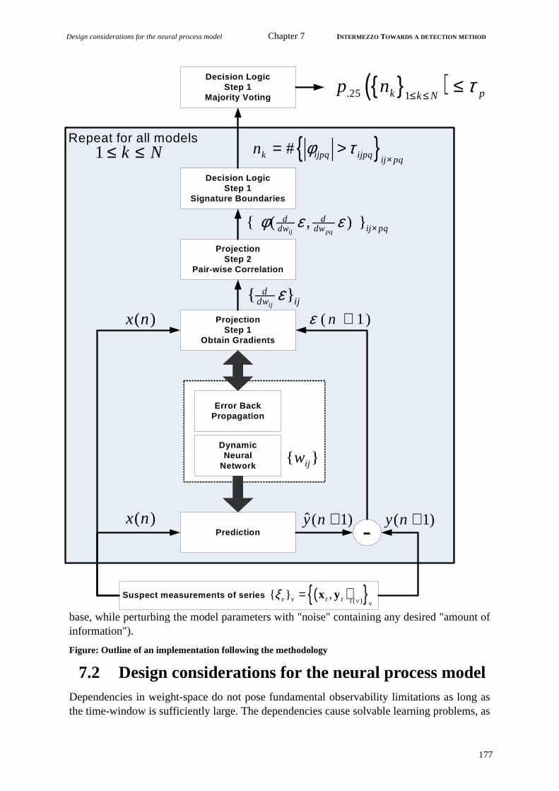
Design considerations for the neural process model Chapter 7 INTERMEZZO TOWARDS A DETECTION METHOD

177

base, while perturbing the model parameters with "noise" containing any desired "amount ofinformation").

Figure: Outline of an implementation following the methodology

7.2 Design considerations for the neural process modelDependencies in weight-space do not pose fundamental observability limitations as long asthe time-window is sufficiently large. The dependencies cause solvable learning problems, as

Repeat for all models

Suspect measurements of series

Prediction -

ProjectionStep 1

Obtain Gradients

DynamicNeural

Network

Error BackPropagation

ProjectionStep 2

Pair-wise Correlation

Decision LogicStep 1

Signature Boundaries

Decision LogicStep 1

Majority Voting

( )x n ˆ ( 1)y n + ( 1)y n +

( 1)nε +( )x n

{ }ijw

{ }ij

dijdw ε

{ ( , ) }ij pq

d dij pqdw dwφ ε ε ×

{ }#k ijpq ijpq ij pqn φ τ

×= > 1 k N≤ ≤

{ }( ).25 1k pk Np n τ

≤ ≤≤

( ){ }( ){ } ,v v t t t v vξ = x y

INTERMEZZO TOWARDS A DETECTION METHOD Chapter 7 Positioning the detection procedure

178

discussed in section 3.4. Research in neural fault tolerance shows that an uncomplicatedlearned mapping can prevent an even distribution of the information across the neural net-work. There is a non-trivial balance in the neural networks topology for optimal learningagainst optimal detection sensitivity. The gradient dependencies should not be inherent to thenetwork topology but rather the result of an interaction between the data and the model. Con-sidering the observability we discourage the use of constraints on the adaptation during thedetection process; yet in the design phase of the model, we too use methods to speed up con-vergence. Procedures to improve fault tolerance in neural networks enhance detection sensi-tivity and stability.

A key conflict to address is between redundancy and optimal statistical risk. We have to ver-ify that the individual model has enough spare degrees of freedom. This is achieved bothempirically through model selection as well as systematically through conventional data anal-ysis from chapter 2. The redundancy can be measured using the pruning metrics described inchapter 3. We have run successful tests for this purpose with OBS, OBD skeletonization andEigen Analysis (SVD) of the weight-space, see also appendix F.

We have analyzed the dynamics of the weights and their dependencies through graphicalinspection of various cases and observed patterns in the dynamics. These patterns suggest thatthe boundaries on the structure in the dynamics for acceptable behavior can be chosen moretightly compared to simple gradient correlations to represent the dependencies; we did notexplore this possibility for three reasons. Firstly, the analysis of higher-order (>2) dependen-cies is computationally expensive, while second-order metrics are minimally required but suf-ficient. Secondly it is hard to see how these dynamics can be captured efficiently with astationary metric without considering large time-windows; we already know from Hessiananalysis that higher-order metrics suffer from convergence problems. Thirdly, reducing thedimension of the monitored metrics on weight-space means using some model of the distur-bances that can occur. The resulting reduction of observability prevents early detection.

Literature and experiments confirm the presence of symmetries in the neural weight-space.There are different solutions that are the same, apart from permutations between connectionsin the hidden layer. Any two models in the set can have identical parts; consequently the com-putation of weight-space metrics for all of the models considering this part is obsolete. Wecan save on computations, possibly through a permutation insensitive similarity-test betweenneural networks based on SVD or EVD on the weight-space.

7.3 Positioning the detection procedureA method that meets the requirements derived in the previous chapter is significantly differ-ent from the more conventional approaches discussed in chapter 4. In order to appreciatethese differences we first have to consider the foundation of detection strategies: key designobjectives and key conflicts between the chosen mechanisms. Characteristic for a detectionstrategy, as discussed in chapter 4, are: 1) the modeling; 2) the (re-)estimation; 3) the signa-ture computation; and the 4) the optimization criteria. Key differences between the closedworld perspective and the open or non-deterministic approach are found in the reliability isprovided. A final criterion for comparison is the result of the detection procedure, rangingfrom an accurate and detailed diagnosis to a mere alarm. The latter requires further supportwith diagnostic analysis. One may find the comparison between conventional and proposedmethod in table 7.1

Positioning the detection procedure Chapter 7 INTERMEZZO TOWARDS A DETECTION METHOD

179

Table 7.1: Positioning the surfacing methodology

Feature Conventional Methods Proposed Methodology

Key Design Objectives

Sensitivity, Promptness, Robustness & Reliability

Observability & Earlinessboth requiring redundancy

Key Conflicts addressed

Sensitivity vs. robustnessPromptness vs. reliability

Redundancy vs. Statistical RiskEarliness vs. Conclusiveness

Modeling Separate model for process and abnor-mality. Reductionistic approach pursu-

ing a single minimal process model from the blueprints. The redundancy is explicit in the fault models and signa-

ture computation. The modeling is two-tier, the models comes from known

principles, as such the parameters can be interpreted.

One behavioral process model which is capable to adapt to vari-

ations. The redundancy is implicit and part of the process model. The modeling is three-tier, there is a non-semantical feature space. The method is

fully data-driven.

Estimation Linear equation solving,Matrix-inversions, linear least-squared, Linear Adaptive Filters, Kalman Filter-

ing.

Error back-propagation in a pat-tern learning setting. Non-linear gradient-based steepest descent.

SignatureComputation

Fault classification from and monitor-ing of coefficients derived from param-eters and residuals, or blind projections

separating null space and signature space.

Boundaries on macroscopic met-rics of the parameter space of a

black-box model, obtained through pattern learning.

Optimization Criteria

False Acceptance RateFalse Detection Rate.

Amplitude of disturbances

Number of samplesSusceptibility to structure in dis-

turbance (profoundness).

Strategy for Reliability

Exactness of modelingIntegrating over time, increasing the

amount of samples required.

Spatial redundancyDiversity of models

Majority Voting

OptimizationProcedure

Relating design parameters, via assumed parametric probability distri-butions to design criteria. The thresh-

olds have a theoretically bounded optimum, only dependent on the param-eters of assumed probability distribu-tions. Graphical support for design is the receiver operating characteristic.

A cleaned database defines nor-mality, signature boundaries and decision thresholds are approxi-

mated based there on.A graphical support relates the amount of structure in residuals

to the response in signature space.

Embedding Conditions

Detection is conclusive for a bounded set of abnormalities

a non-conclusive method, hence an additional impact analysis is

required

INTERMEZZO TOWARDS A DETECTION METHOD Chapter 7 Positioning the detection procedure

180

The procedures discussed in this intermezzo (chapter 7) are not part of the theory. They areprovided without further argumentation or proof. In chapter 8 we argue and illustrate thepotential of neural modeling and estimation to meet the modeling requirements. The illustra-tion of the proposed detection principles can also be found in chapter 8.

Feasibility of modeling for early detection Chapter 8 NEURAL ABNORMALITY DETECTION

181

Chapter 8

Neural Abnormality Detection

In the ordinary quasi-regular roaring and steaming of the machines in a pro-duction plant, a weak but different pattern emerges just before the erraticunstructured variations occur. Hardly noticeable for the human eye, betweenthe ignored seemingly random flickering of LEDs on the operators controlpanel some weak correlation emerges … is it interfering with the regular pat-terns associated to the normal behavior, will it degrade performance? Sev-eral species in an ecosystem coexist, apart from the quasi random births anddeaths, happily eating or less happily being devoured … then it seems a newquasi-periodicity appears. Is a new species emerging and interfering withthe existing populations? Is it possible to isolate an emerging profound inter-ference from the quasi-regular time-varying behavior without relying on a,possibly oversimplified, system structure? The neural black box capturesdynamical patterns from data, and is adaptive as well. Hence it is capable ofspotting harmful trends in a non-stationary system. Is this the required elas-ticity in complexity? And if so, is there any way of computing stable yet sensi-tive signatures from neurons that are in isolation far too erratic?

Chapter 8 discusses neural features in relation to the derived requirements. We consider, in sec-tion 8.1, whether the properties of neural networks comply with the requirements from the pre-vious chapter. We find out how to derive the stable signature from a neural parameter space insection 8.2. Illustrative experiments of early detection of profound abnormalities with neuralnetworks, discussed in section 8.3, have been published at ProRisc'01. Section 8.4 discussessome recent publications in our problem domain to clarify the difference between our perspec-tive and other different attempts to overcome some of the known issues in detection.

8.1 Feasibility of modeling for early detectionThe modeling requirements for early detection resemble properties of neural networks. Someparticular observations indicate that neural models can capture dynamics of specific instanceswithout loss of general accuracy. Redundant degrees of freedom are not necessarily harmful orresult in obsolete parameters. Neural networks offer different solutions of similar accuracy.Universal approximation is implemented by neural networks. A limiting factor is the learningprocess that can be overcome by a posteriori model selection.

8.1.1 Data-driven dynamic modeling

Neural networks are suitable candidates for early abnormality detection. We will illustrate thisby considering neural modeling capabilities compared to necessary properties for data-drivendynamic modeling:

NEURAL ABNORMALITY DETECTION Chapter 8 Feasibility of modeling for early detection

182

data-driven-ness: the model behavior is determined by data. The internal structure ofthe system needs not to be known or coded in the internal structure of the neural model,i.e. the system can be considered as a black-box.

universal approximation: Any dynamic behavior can be approximated by the structureof a dynamic neural network, provided sufficient neurons are provided.

universal learnability: any structure can be estimated from data.

extrapolation: it is possible to predict behavior using a dynamic neural model and suffi-cient data representing the current state of the system.

Neural networks are connectionistic models that can represent a mapping without designingthe internal structure. The capability (e.g. VC-dimension) of the model is determined by thecoding of the problem (input-output representation, e.g. delay-lines and feedback) and thenumber of hidden units. In the coding we can at least prevent an under-estimation of the time-window through data analysis, while there are also some well-known coding aspects (subsec-tion 2.2.2). With regard to the estimation algorithms discussed in chapter 3, we can concludethat the neural function is determined by parameters. These parameters can be optimized forthe data. The neural function is then fully data-determined provided it has sufficient degrees offreedom. As for the selection of hyper-parameters (number of neurons, learning parameters)we can rely on heuristics and emperical procedures. Neither the fitting procedures nor the neu-ral archtiecture requires any knowledge of the internal structure of the generating process.

A neural network can be used with arbitrary precision to approximate for static functionapproximation [Cybenco, 1988; Hornik, 1989]. This means that the smallest possible error canbe achieved with a representation of a function by a Multi-Layer Perceptron, with just one hid-den layer. Universal approximation for finite impulse response behavior is possible withfocussed feed-forward neural networks. These present a finite time-window (memory) fol-lowed by a static feed-forward neural network [Mozer, 1994]. This has been shown particu-larly for gamma neural networks [Sandberg and Xu, 1997; Principe, 1992].

Given a time-series (trajectory) generated by a feedback system with a cyclic infinite impulseresponse, a generator for the limit cycle followed by a feed-forward neural network canapproximate with arbitrary precision the dynamic behavior represented by the time-series[Zegers et al., 2003]. The universal approximation, i.e. approximation with arbitrary precision,of continuous-time neural networks has been shown [Funahashi and Nakamura, 1993]. We areconsidering only discrete-time neural networks, but the discrete neural network representationcan approximate continuous-time behavior as closely as desired. We conclude that dynamicneural networks based on a Multi-Layer Perceptron, with dynamic extensions as presented inchapter 3, can approximate any dynamic behavior with arbitrary precision. However this doesnot guarantee that the most suitable representation can be found from data with any procedure.

We cannot state universal learnability in neural networks, as this is not guaranteed. Howeverthe limitations of learnability are much better understood (chapter 3). This helps in selectingthe appropriate architecture for the data at hand. Neural design issues are: conflicts in the dataand undecisiveness [Barakova, 1999] and cancellation as a result of an unfortunate architec-ture. However in practice dynamic neural networks have been demonstrated to perform asgood as or improve conventional models in representing dynamic behavior. Sample represen-tation and learning reconfiguration through randomness and architectural modifications aresuitable remedies for the design issues. Provided a viable neural architecture is chosen, a com-

Feasibility of modeling for early detection Chapter 8 NEURAL ABNORMALITY DETECTION

183

bination of annealing and randomness converges to a statistically optimal solution. The itera-tive learning process (error back-propagation) can be improved and there are many alternativesnowadays. Suitable heuristics to do so vary in step-size, momentum and add randomness to thelearning process.

Using dynamic neural networks as a regression model (chapter 3), the capabilities to extrapo-late a time-series are limited to the time-dependent variables. The variables that are truly inde-pendent of time can never be predicted, but the time-dependent variables can be predicted by asuitable neural model. To detect abnormalities, the coding must be such that all time-dependentvariables are input as well as output to the model (AR). The step-size of the prediction dependson the coding. A 1-step ahead predictor is enough to generate a complete series, but improve-ments in the estimation of the model are achieved using a multiple step ahead predictor. Theusual dynamic modeling limitations for prediction/extrapolation are no different for dynamicneural networks: rapid loss of accuracy, confusion from deterministic cross-overs and depen-dency on initial conditions (chaos). We conclude that there are no fundamental limitations forextrapolation from a dynamic neural network with respect to the AR variables.

8.1.2 Soft-scaling complexity

Complexity estimation (subsection 2.4.5) provides a fairly unique optimum for the number ofparameters for conventional modeling. However we have seen that complexity is less fixed inneural networks (chapter 3) and can be scaled-up if the need arises. Indeed the scaling com-plexity is a very fundamental property. At the start of a learning process the neural network israndomly initialized and represents no particular structure. Such a neural network has thepotential to learn a simple linear dependency between input and output, but it can also learnmappings that are much more complex. There are four necessary properties for the soft-scalingcomplexity in dynamic neural networks:

• A neural network can adapt to the complexity of a static functional mapping

• A neural network can adapt to temporal depth and resolution of a dynamic dependency

• The relevance of the network weights in the contribution of the mapping can be enforced

• The redundancy is not harmful in finding a mean optimal representation

A neural network can adapt, through learning, to the complexity of a static functional mapping.The neural network is not built with components that are distinct, i.e. the behavior of the neu-rons in the neural network is not orthogonal. An input-output representation, in particular, isobtained through a combination of uniform functions (sigmoids). The number of neurons is notthe only factor determining the complexity of the functions that can be approximated. A neuralnetwork capable of approximating a very complex mapping with many dependencies betweenvariables and at a high polynomial order is also capable of accurately representing the lesscomplex mappings. The complexity of a mapping is foremost determined by the weights in aneural network, by the activations across the sigmoid, and by the dependencies between thedifferent neurons. As long as the neural network is not saturated, additional structure can be fit-ted in the model. These are the generalization and plasticity properties in a neural network.

NEURAL ABNORMALITY DETECTION Chapter 8 Feasibility of modeling for early detection

184

Figure 8.1 : Adaptation throug time in a hot-strip mill, with MATH) MM-the physical-principle model;2) M0: a neural network without on-line adaptation; 3) OLB: a neural network with on-line adaptationfrom scratch in every batch; 4) OLR: a neural model which is continuously adapting.

An illustration of this capability is the hot-strip mill experiment. First taking the entire data set,we find a model that is the best model on average for all instances of the process behavior. Thelearning converges although there are conflicting variations in the data. The resulting networkhas no particular bias, since the samples are randomly taken through time across all instances.We can see in the residual for any particular batch that there is remaining structure ... thebehavior that is present across all instances (batches) of the process is less complex than thestructure present in different instances. Yet we see [van der Steen, 2002], that the neural net-work can adapt through time across the different instances, taking the observations in thebatches one-be-one. The structure in the residual of the best average model is removed throughon-line learning. This is the case across a large amount of batches, each batch corresponding toa different instance of the hot-strip mill. Hence we conclude that increasing complexity issmoothly accommodated while the generic and common features are stably stored without lossof plasticity. Moreover we can also conclude that the representation with a neural model ishighly redundant, since the adaptations in the equilibrium are strongly dependent, i.e. thedegrees of freedom in the neural network have not been used to the fullest extent. Analysis ofthe behavior of the neurons reveals that pairs of neurons collaborate: on some parts of the inputdomain they correlate strongly (both positive and negative correlations occur). We will explorethese features more extensively in a laboratory-setup in subsection 8.2.3. Increasing complex-ity of mappings can be fitted by an MLP. The complexity is limited but not determined by thenumber of neurons, but by use of the sigmoid (distribution of neuron activations). There is noclear boundary in neural complexity. The design problems in 3.4 are now to our benefit.

Feasibility of modeling for early detection Chapter 8 NEURAL ABNORMALITY DETECTION

185

Now we have to consider whether neural networks are also capable of adapting smoothly toemerging structure at different time-lags? The neural network with infinite impulse response,through feedback, has singularities in it’s adaptive behavior since there are poles in it’s input-output mapping. Can these be controlled for any system? We have presented focussed time-lagged neural networks in section 3.2. These networks have no internal feedback; the time-window is presented as a static input to the neural net as a tapped delay-line. In this way theneural network can discard any redundant lags by setting the weights associated to the taps toapproximately zero. Alternatively the coefficients for the taps can be estimated in differentways, e.g. by temporal component analysis [van Veelen, 1999].

Figure 8.2 : Set-up of an identification experiment with a signal generator (left) and the observer (right)The temporal depth/resolution is modulated smoothly through time in the signal generator, while the tem-poral depth is estimated from the on-line adaptation in the gamma tapped delay-line and the static MLP.

Soft-scaling adaptation through time demands a time-window as large as required for the data.The use of feedback facilitates comparing behavior with a fixed number of parameters even iftemporal depth in data varies. A trade-off can be made through on-line adaptation on databetween temporal-depth and temporal-resolution while universal approximation is stillobeyed. Such a solution has been described (subsection 3.2.4): the gamma networks show thatwith a fixed number of nodes the temporal depth can be adaptive, while the nuisance of polesaffecting the stability of learning is prevented by sharing feedback parameters across thedomain. We can illustrate this capability with the following setup. We take a gamma tappeddelay-line followed by a non-trivial non-linear, yet reversable mapping represented by a staticMLP (figure 8.2). The that controls the feedback is smoothly modulated. The non-linearmapping as well as dynamics are estimated and tracked from the generated data. The typicalbehavior for the simultaneous estimation of and the non-linear static mapping by an MLP isshown in figure 8.3. This illustrates the capacity of a gamma neural network to adapt to vary-ing temporal depth.

µ

µ

NEURAL ABNORMALITY DETECTION Chapter 8 Feasibility of modeling for early detection

186

Figure 8.3 : Results from the gamma-tracking experiment. The actual (straight line) and the esti-mated (dotted line) through are plotted against time.

The final aspect of soft-scaling complexity to consider is the relevance. Smooth scalingimplies a non-discrete emerging structure. The parameters need to represent the novel structureof the original input-output mapping. This is not the case if signal-components in the model aresimply switched on and off. This property is non-trivial if the neural network is redundantbefore the complexity of a dynamic mapping increases. However, firstly, we have identified inchapter 3 the mechanisms that ensure the information distribution in a redundant model. Thesemechanisms are the techniques for complexity regularization (section 3.4). Secondly, the col-laboration among connections (weights) can be observed, even without the complexity regu-larization. The correlation between gradients (weight adaptations) in an equilibrium isapproximately uniformly distributed, which means the degrees of freedom are constrained bythe mapping in the data. There are almost no weights that behave as independent parameters.Typically 1 weight is not the statistical equivalent of 1 parameter, or 1 degree of freedom, andit is this remarkable feature that allows to accommodate abnormal emerging components.

The collaboration between neurons in neural networks has been investigated extensively. Tak-ing a stochastic approach the dynamics of weights can be described using the Fokker-Planckmodel. This approach has been applied to equilibria [Leen and Moody, 1993] and to transients[Orr and Leen, 1993] in the learning process. The stochastical learning model originates fromthe work of Amari, and has rigorously been followed by Heskes and Wiegerinck. Neural train-ing problems can be understood from the dependencies in the networks, i.e. revealing whetherthe optimization problem is ill-posed, as indicated by the rank-deficiency measured by Eigenanalysis of the Jacobian and Hessian [Saarinen, Brameley and Cybenco, 1991]. In a similaranalysis, SVD has been applied to determine and improve the fault tolerance of Multi-LayerPerceptrons in a pattern recognition application [Emmerson and Damper, 1993]. Fault-toler-ance is analyzed considering the internal reduncancy. SVD is used to assess the redundancy. Itis concluded that simply adding hidden neurons does not automatically improve fault-toler-ance, but the error back-propagation tends to distribute the information evenly over the net-work, i.e. no single neuron codes a particularly distinct feature. An even distribution ofinformation in the neural network is believed to improve the generalization and the fault-toler-ance. A strategy for even distribution is based on three imperatives [Minay and Williams,

µµ

Feasibility of modeling for early detection Chapter 8 NEURAL ABNORMALITY DETECTION

187

1994]: 1) each neuron should be as irrelevant as possible (maximum irrelevance); 2) each neu-ron should be as relevant as necessary (minimal relevance); and, 3) the relevance of neuronsshould be as uniformly distributed as possible (uniform relevance). A proposed technique toachieve this is to train with noisy data. The information distribution can be improved byincreasing the training time, though this increase hardly brings an improvement of the meanerror. This follows from a study of the effect of training on the fault-tolerance of neural net-works [Nijhuis, 1990] concluding that training time has a positive effect on the informationdistribution in the neural network. Neural networks can also be made fault tolerant by itera-tively adding degrees of freedom when the over-complexity is regularized through constraintsto guarantee generalization [Edward and Murray, 1998].

8.1.3 Common features from multiple instances

The capacity to generalize over different instances and to store the common structure in a sta-ble fashion, while not loosing the capacity to adapt to structure, can be found in particularinstances. This is a non-trivial feature of neural modeling. Various researchers have argued,taking a classical statistical attitude, that memorization (storing instance specific information)is harmful to the overall performance of a model. Over-training and memorizing patterns at thecost of generalization and plasticity indeed have a statistical theoretical basis and experimentswith artificial data can proof that the statistical risk can increase when there are too manydegrees of freedom in a model. We have two claims on the use of neural networks in practicaland realistic cases:

• The redundancy is not necessarily harmful;

• A stable fit of common features is possible without loss of plasticity and generalization.

Redundancy in a neural network is not as simply identified, as 1 weight is not 1 parameter isnot 1 degree of freedom. Firstly the redundancy is not necessarily harmfull since the neuralmodel has soft-scaling complexity, i.e. through collaboration (strong dependencies) the effec-tive degrees of freedom are decreased as can be observed in the dependencies among weightsand among neurons. Secondly, the redundancy is not necessarily harmfull, because the redun-dancy can be controlled through regularization mechanisms (section 3.4). Thirdly, the ratio ofavailable data against number of parameters is in practice quite healthy. A 1:10 ratio is anaccepted rule-of-thumb, e.g. in the Corus case and in the telecom example the ratios are examples vs. weights. Fourthly, the true usage of the redundancy becomes measurablethrough several metrics for regularization and pruning discussed in chapter 3. Therefore theharm can be measured and controlled. In the hot-strip mill case we do see that the adaptationthrough time helps to accommodate structure emerging in the residuals, while adaptation toany particular samples does not decrease the error of the model on the whole ... unless theycontain persistent changes (i.e. also the common features vary on the long run). In the hot-stripmill case the long-term validity of the model (common features that are present on the long-term) has been verified after adaptation continously when new data arrive:

1. the error of the model on old data is inspected. This reveals a decrease in the perfor-mance of the model to explain the old data, but the validity on a sequence of production batches does not decay rapidly.

2. the capability of rapidly adapting to the old data is checked by adapting on a pattern-by-pattern basis. This reveals that the model is capable of rapid recovery to explain historic

105

103

NEURAL ABNORMALITY DETECTION Chapter 8 Signature computation

188

data after adaptation to newer data. In this case, the variations over different instances can easily be adapted while common features are captured without decay, by adaptation.

The various practical examples, where large volumes of data are present and the variation inthe data comes from different instantiations of a system with some invariant dependencies,show that memorization and over-fitting in neural networks do not give a problem.

8.1.4 Meeting modeling requirements for early detection

We have shown the capability of neural networks for predictive data-oriented modeling with asoft-scaling model complexity. A combination of regularization and re-estimation enables theneural model to learn and preserve common features across multiple instances. The iterative orpattern-learning algorithm allows for early detection, while the capabilities to extrapolate andpredict from a dynamic neural network allows for impact analysis. The signature computationcan be designed to use a minimal number of observations, since the training can be iterative(instead of requiring complete batch learning averaged over a complete time-series). The onlylimitation for the number of samples in the impact analysis is the number of chosen lags. Wecan also provide certain conditions, enforcing that the learning is an information-preservingmapping to the weightspace. This fulfils the requirement on estimation that the structure in theresidual is preserved in parameter adaptations. This is quaranteed if the weights are observablein the input-output behavior of the neural model. The observability of weights corresponds totheir controllability. Hence the preservation of information holds if any dependencies betweenweights are constrained by the data. This feature is measurable. It holds if all information in theneural model is learned from data and if the learned mapping can be fully unlearned e.g. bypresenting random data. Finally, we come to the capability of neural models to be distributedand easily scaled-up. This is essential for monitoring behavior in distributed and evolving pro-cessing networks. We conclude that the architecture of the neural model (MLP based) togetherwith the nature of the learning in neural networks (EBP based) makes the neural modeling suit-able for early detection. We have illustrated the presence of necessary features in the neuralmodeling for early detection modeling. Some possible limitations must be considered to graspto what extend these provide sufficiency. The conditions on neural modeling and signaturecomputation have to be considered from the perspective of neural features (3.4.1), as there arestill some peculiar issues in designing a neural network. There are also some fundamental lim-itations on modeling for detection (4.4.2). These apply to any modeling approach, both neuraland conventional. Considering only the requirements on modeling, we see that the neural mod-eling overcomes the limitations of conventional approaches. Since neural networks have soft-scaling redundancy, they meet modeling requiements of risk-invariant redundancy.

8.2 Signature computationGiven neural modeling meets the modeling requirements, we still have to address the issue ofsignature computation from neural models. Recall that the objective is to compare the differentmodels which correspond to two representations of the potentially differing system. In the sig-nature space the effects of randomness, acceptable variations and system changes must be sep-arable by design. The possible inputs for signature computation are data-space, residue-spaceand parameter-space. In section 8.2.1 a survey of neural metrics that can be used for signaturecomputation are summarized. In section 8.2.2 we select the suitable signature computation for

Signature computation Chapter 8 NEURAL ABNORMALITY DETECTION

189

early detection. Section 8.2.3. is an illustration of the capability of early detection with neuralnetworks.

8.2.1 Survey of neural metrics

In chapter 4 we have presented three methods to compare models: directly from their input-output behavior, through their residuals, and through their parameters. Similarly to the analysisof learning behavior of neural models, we find metrics based on:

• input-output behavior;

• the residual or error, such as shown in learning curves;

• the weights or error as function of weights (error-surfaces).

In section 3.4, table 4-6, we discuss procedures for treating some of the neural design issues,which are the origin of neural metrics for analysis of the neural model.

• Optimal configuration of the learning process: initialization, stopping criterion, adapta-tion of learning parameters (learning rate, momentum, jittering)

• Optimal complexity for accuracy, stabilility generalization and fault-tolerance: regular-ization, selection of hidden layers and neurons, input-output coding, analysis of the reli-ability.

• Analysis of solvability, detecting learning problems due to: coding (ill-posedness), stag-nation, cancelation effects.

In all these procedures the assessment of the smoothness of the error-surface is essential. Thisis particularly hard due to the high-dimensionallity of the weight-space and the data dimension& non-stationarity in real-world problems. The relation between the internal representation ina neural network and it’s external behavior is essential to improve quality and performancethrough these procedures. The metrics in 3.4 are categorized in the way this relation is esti-mated:

• Microscopic: local metrics per connection or neuron. Examples from chapter 3 are Neu-ron sensitivity, Local Relative Sensitivity Index, Mozers Neuron Relevance, Weightvariance, the momentum term, and data-dependent adaptive learning rates described intable 6.

• Macroscopic: global dynamics. Examples are the error-surface itself, the higher-orderexpansians such as the Hessian, the from the conjugate gradient, OBD Saliency, Bar-tlett’s information theoretic relevance. Transition matrix in a Markov-process approxi-mation, energy and entropy in the Fokker-Planck approximation for learning behavior[Haykin, 1990; Heskes and Wiegerinck, 1996].

• Condensed: characteristics derived from macroscopic behavior: e.g. rank-deficiencycondition numbers, complexity, controllability, Akaike information criterion (subsection2.4.5)

Microscopic metrics consider typically statistics of weights or gradients, ignoring the depen-dencies. They are computationally cheap and can be used locally for adapting the learning orthe model. Since they ignore dependencies in the model they are called first-order metrics.

β

NEURAL ABNORMALITY DETECTION Chapter 8 Signature computation

190

Macroscopic metrics come in a larger variety. They also measure the interaction within themodel. Exact computations of macroscopic metrics such as the Hessian are computationallyexpensive, as the local error-surface is explored in a vast number of evaluations for differentweight perturbations. Such a sampling of the weight space is pursued in a Bayesian approachwhich is reasonable when it replaces the iterative learning. The inverse Hessian is approxi-mated in OBD to estimate saliency of neurons or weights. The OBD algorithm [Haykin, 1994]uses an iterative approximation with series of Jacobian vectors (dE/dw) as only input. We haverepeatedly encountered convergence problems with this approximation, particularly outsidethe equilibrium. Though a statistically sound theory for stochastical dynamical modeling oflearning behavior is provided [Heskes and Wiegerinck, 1996; Amari, 1990], the theory onlyapplies to very “normal“ data and highly-constrained models and learning processes. Non-Gaussian gradient distributions and data-dependent gradient dependencies occur. This seem-ingly Brownian motion in weight-space prevents some intricate higher-order metrics, yet it isan effect of the data. The fault-tolerance analysis through an SVD on snapshot of Jacobians (asequence of dE/dw vectors) in an equilibrium [Emmerson and Damper, 1993] re-appears fre-quently in neural networks analysis. We have observed in several cases that the SVD on snap-shot of Jacobians is much more robust than Hessian approximations.

Condensed metrics characterize the neural model behavior when the data variations are aver-aged out or only stationary processes are considered. Often they require the reliable estimationof a macroscopic measure, such as the SVD of a series of Jacobians or Eigen-values of theHessian, or the rank of the observability matrix. Though these types of metrics are robust withrespect to noise, they offer only a one-dimensional view on the system which is not enough toisolate different types of dynamics resulting from variations in the modelled process.

8.2.2 Selection of metrics

We have to consider the possibility to extract unique and stable signatures from neural net-works, despite the fact that the weights are non-unique and non-semantical. In case of abnor-malties the error surface of a model will change as illustrated in figure 8.4.

Figure 8.4 : The error-surface of a model for a particular data-generating process (non-dashed line)with a particular equilibrium. When the process changes, the error surface changes. Particularly theequilibrium will not remain on the same location (dashed line). Hence the dynamics specific to the originalequilibrium will change significantly.

Signature computation Chapter 8 NEURAL ABNORMALITY DETECTION

191

We seek a metric on the weight-space that captures such a change in the error-surface in theequilibrium, thereby fulfulling the necessary requirements on signature computation:

• Inherent change in behavior of model parameters, i.e. the signatures do not add redun-dancy in the form of additional degrees of freedom. Particularly the signature computa-tion does not contain any additional information of the modelled system. Ideally thereshould not be any bias for particular types of disturbances.

• The signatures need to enable a comparison of two models that correspond to two (pos-sibly different) instances of a system, even if the system’s behavior has increased in com-plexity. For reasons of computability we assume a fixed and finite number of parameters.

• Robustness and stability are required despite acceptable time-variant behavior of thesystem. Moreover the acceptable variations must be separable from potentially harmfulldisturbances in the signature space.

• A fair trade-off between scope and the earliness of the response. The number of samplesused for the signature computation must be minimized for a certain confidence level.Though the model can cause limitations in the observability of the parameter space, thestructure in drift observable from the residual in the time-window must be preservedbecause it is relevant for system performance.

Figure 8.5 : A gradient-gradient plot in an equilibrium for a pair of connections in the hidden layer.

The neural metrics and the models of learning discussed in the previous section have been con-sidered for signature computation [van Veelen, 2000]:

• First-order neural metrics do not offer sufficient stability. The behavior of singleweights, i.e. their distribution function, does not allow detection since a threshold forseparating noise and acceptable behavior cannot be chosen such that profound distur-bances are detected. The experiments [van Veelen, 2000] illustrate a limited performanceof first-order metrics: 1) the threshold for the gradient of single weights, while monitor-ing all the weights, either generate too many false alarms or too many misses; 2) a testwhether the distribution of the gradients is Gaussian or remains Gaussian is not suitable

NEURAL ABNORMALITY DETECTION Chapter 8 Signature computation

192

for detection while a Lillifors test is used as white-noise test with equal mean and vari-ance; 3) a comparison of the distribution of gradients for known and new data through aKolmogorov-Smirnov test does not allow to distinguish acceptable variations from pro-found disturbances.

• Condensed metrics do not offer the required sensitivity. Averaging over large time-windows and many variables, e.g. weights, limits the observability or scope. The dynam-ics within an equilibrium: 1) are not reliably estimated without a sufficient amount ofdata when represented in a single metric; and 2) do not necessarily effect changes intocondensed metrics such as the complexity of the mapping. Nonetheless they can be avaluable addition to a reliable estimate of fundamental change in the system. In physical-principle models abstract, non-measurable properties, e.g. mechanical wear, have noaccuracy if the nominal system model is poorly identified.

• Parameters for theoretical models of learning behavior are not suitable in practice;e.g. Fokker-Planck. Linearized models such as EKF and Markov Processes do not bene-fit from the non-linearity by having redundancy in the model. Second-order learningrules (Gauss-Newton, Conjugate Gradient etc.) are acceptable for fitting the model.However they cannot be used to map the residual to the parameter space with preserva-tion of structure. Limitations for these models and associated learning procedures are: 1)computationally expensive; 2) dependent on Gaussianity assumptions; 3) require con-straints on the learning process which seriously limit the observability (i.e. batch ratherthan pattern learning). Higher-order metrics are required. The dependencies between thegradients need to be measured in an equilibrium.

Figure 8.6 : The distribution of gradient-correlations in a neural model for a Volterra-Lotka system inthe equilibrium, i.e. converged to a noise level, horizontal axis is [0 1]. This shows strong dependenciesbetween gradients; these are typical dynamics in the equilibrium.

• Second- and higher-order metrics on the weight space. The dynamics are revealed bya gradient against gradient plot. An example is shown in figure 8.5 for a sine-wave pre-diction model. The dynamics in an equilibrium are characteristic for the data in relationto the model. Intuitively such dependencies as measured by second-order metrics mustbe stable yet sensitive. We propose to measure the dependencies between all the gradi-ents in each hidden layer of the neural model, because metrics such as approximateinverse Hessians do not provide stable detection responses unless averaged over largetime-window at the unacceptable loss of earliness. These gradient dependencies can becharacterized by correlation or mutual information. Figure 8.6 shows the distribution ofthe correlations of the gradients. The use of metrics with more than 2 variables, i.e.

Computer experiments Chapter 8 NEURAL ABNORMALITY DETECTION

193

higher than second-order dependencies are discarded because of poor numerical stabilityand computational complexity.

Parity analysis in the residual space aims to find a null-filter sensitive to change. However theparity relations are derived qualitatively from a white-box system model, which we cannot relyon. The projection on the state space model (equation 4.25) is in fact a null-space of the modevariables. This null-space is very similar to finding the null-space of the weight-space, e.g.using SVD. The second-order metric of the vector of all the pair-wise gradient dependenciesper hidden layers is more simple, and numerically more stable, than a Hessian metric. Yet itcan represent the dynamics, like curvature in the equilibrium, sufficiently. We consider againthe requirements on signature computation for Full Gradient Dependency metrics (FGD):

• The FGD monitors inherent change in the behavior of model parameters. There is notan a priori model on the designers knowledge or data-dependency in the way that signa-tures are computed from the model parameters; there are no additional degrees of free-dom in the signatures.

• The FGD enables a comparison between two instances of system behavior since onlythe gradients have to be computed in the equilibrium; the weights do not actually change.

• The stability of the dynamics in the equilibrium depends highly on the distribution of thedependencies between the gradients. Considering the set of all dependencies simulta-neously allows for a reliable detection of significant changes in the overall, high-dimen-sional, error-surface. Effective redundancy in the neural network, measureable through aplot (figure 8.6), improves the detection reliability. Since the FGD represents the dynam-ics for the whole weight-space in the equilibrium, it is sufficient because higher-ordermetrics lack stability. FGD it is the most stable un-biased metric. Moreover a set of dif-ferent neural models can be fitted to the database. Diversity in the model set willimprove the reliability through voting strategies and is suitable to identify blind-spots.

• A trade-off between scope and earliness is necessary and possible with FGD. The sta-tionary window for the gradient-depencies can be determined from the data using differ-ent thresholds for false alarm probability and blind-spots. Blind-spots can be measuredby perturbation analysis using the neural network model as a simulator for the system.

The signature computation is not the cause of limited scope or observability, so observabilityis a challenge for modeling. For several types of disturbance we can check whether the modelis able to adapt to the changes in the system, i.e. sustaining the model quality. If the model canadapt, then the changes are observable in the weight-space of the model.

8.3 Computer experiments In this section we illustrate the principle of non-deterministic detector design with neural net-works using two examples. In the first example we discuss the design steps one by one, whilein the second experiment we focus on the results.

8.3.1 Illustration of the design with a sine-wave prediction example

The system and it’s disturbances.

We take a time-series made up of a single sine-wave with additive white noise. There is addi-tive noise at 1% of the sine amplitude. Injected disturbances are: 1) yet another 1% white

NEURAL ABNORMALITY DETECTION Chapter 8 Computer experiments

194

noise; 2) 2% white noise; 3) a sawtooth at noise level; 4) a block wave at noise level; 5) slightfrequency modulation; 6) an additive harmonic sinewave at 20% of the noise level (1% ofsine). A simple threshold on the residual shows that the structural disturbance cannot be distin-guished from random noise, i.e. the residual is unsuitable for early detection.

Phase 0: Data analysis.

Data analysis was obsolete in this case. The number of time-lags corresponde to approximately of the period of the sine-wave, have been used for a one-step ahead prediction.

Phase 1: Model design.

We have used 25 models in a cross-validation set-up. The stopping criterion was trivially deter-mined. As in the artificial examples we know the noise floor, so the stopping criterion was avariance in the prediction error of corresponding to a noise amplitude of .

Phase 2: Detector design

Step 2.1: Verify that accommodation of the changes is possible with the set of models.We have checked that the error is minimized to the original level for each of the size per-turbations on the original process. The demonstrated models are capable of adapting tothe disturbance. Hence the disturbances will be observable in the weight-space.

Step 2.2: Find the stationary window and the boundaries of the gradient correlations.We can verify the stationary window for the statistics: it approximately corresponds tothe highest frequency component in the time-series. In this case 32 datapoints are suffi-cient. A rather ad-hoc boundary per gradient correlation pair is chosen: 0.03. Theboundary is quite tight such that it is easily exceeded, even for acceptable variations.This interacts with the fraction threshold chosen in the next step.

Step 2.3: Determine the fraction threshold. The last design parameter to select is thefraction of gradient correlations which should cross the threshold before an alarm israised. We have just inspected if such a boundary can be chosen using as an upperboundof the 2% additiative noise. For now we only need to verify whether we can distinguishthe changes in the process generating the time-series.

The results are shown in figure 7.7. The boxplot shows the fraction of gradient correlations thatare out of bound for the 25 models used in the experiment; the frequency shifts and the modu-lated perturbation is detected with the highest confidence. The shifted as well as the additiveharmonic disturbances are easily isolated from one other by thresholding. These results havebeen reported in [Veelen, 2000]

1 4⁄

104–

102–

Computer experiments Chapter 8 NEURAL ABNORMALITY DETECTION

195

Figure 8.7 : Results from the sine-wave generator perturbations experiment. Persistent and profoundperturbations such as a frequency modulation (shifted) and an additive harmonic (sin) are easility iso-lated from the additive disturbance (block and sawtooth).

8.3.2 Robust non-deterministic detection for a Volterra-Lotka system

The system

We have selected the Volterra-Lotka system, also known as the preditor-prey system. It is themost simple system that exhibits all the typical interactions of multiple entities sharing an envi-ronment. The interactions between the entities can change similar to the complex real-worldsystems we have discussed. Furthermore, with this artificial system we can study all typicaldisturbances associated with: 1) acceptable variations; 2) disturbances not inherent to the sys-tem (e.g. sensory perturbations); 3) non-persistent changes in the dynamics (temporary pertur-bations of the state/mode of the system); and, 4) chronic disturbances resulting from persistentsystem changes (persistent change in the state transitions of the system). The Volterra-Lotkasystem is described by the following two equations:

(8.1)

(8.2)

where and represent prey and preditor resp., the fraction of the population shot byhunters per time-unit; and represent natural growth, decay of the two populations; is the

x·1 t( ) rx1 t( ) αx1 t( )x2 t( )– x1 t( )u1 t( )–=

x·2 t( ) βx1 t( )x2 t( ) cx2 t( )– x2 t( )u2 t( )–=

x1 x2 uir c α

NEURAL ABNORMALITY DETECTION Chapter 8 Computer experiments

196

fraction of the prey eaten per preditor and is the off-spring of the preditor population perprey hunted. Notice the non-linear interaction between the two populations.

Figure 8.8 : A time-series generated by the volterra-lotka system described in equations 8.1 and 8.2.

Each time-series contains 1024 data points. We have trained 20 models until the RSE becomesstable; the systems have not been exactly identified. However they provide an accurate one-step ahead prediction.

Disturbances

Each disturbance has been chosen such that the net effect on the amplitude of the signal isbelow the known additive noise level, which is the noise added to the system observables. Sim-ilarly to the previous experiment the disturbances cannot be distinguished using a threshold onthe residual. We have simulated the system with three kinds of disturbances.

Sensory disturbances. The system itself is not affected by these types of disturbances. Wehave applied for the additive disturbance: sawtooth signal, random noise and block-waves with at most 5% of the signals generated by the system. The observed series aresimulated sensory variables with the additive disturbances .

(8.3)

Mode perturbations. The second kind of disturbance is the mode perturbation. These dis-turbances are simple additive noise, but with a sustaining effect, i.e. the mode is actuallychanged with impact on the time-evolution of the system. The mode perturbations arewhite noise with amplitudes of 0.1%, 0.5% and 1.0% of the original signal.

(8.4)

Inherent system change. The third kind of perturbations are slight changes in the tran-sition parameters , , and . The changes in these system properties where 5-10%,while the trajectories generated were all within the possible set of trajectories of theoriginal system with the used noise level.

β

yi ε t( )

yi t( ) xi t( ) ε t( )+=

x′i·

x·i εi t( )+=

α β c r

Computer experiments Chapter 8 NEURAL ABNORMALITY DETECTION

197

We have verified that each of these disturbances can be accommodated by the models in theset. Apart from the discontinuities in the disturbances we have encountered no problems. Weconclude that the disturbances are in principle observable in the weight-space. The key capa-bility to verify is the ability to distinguish the disturbances based on profoundness, wheremode perturbations are more profound than sensory disturbances, and inherent system changesare more profound than mode perturbations.

Results

Figure 8.9 : Boxplot of th fraction of out-of-bound gradient-correlations for 20 models of the Volterra-Lotka system with different kinds of disturbance: sensory disturbances, mode disturbance and perturba-tions of the coefficients.

Again, the signatures are the fraction of out-of-bound gradient-correlations. The boxplot in fig-ure 8.9 shows the results of the experiment. The three kind of disturbances are clearly observ-able as well as separable in the signature space. The stability of the response, with a varianceover the 20 models, is sufficient to have a confident separation between the three kinds of dis-turbances. This proofs the early detection principle of neural networks for systems that havenot been identified through exact modeling.

Observations

We have investigated graphically the weight-space of the neural models for the Volterra-Lotkasystem. In figure 8.10 the gradient vs. gradient plot for a few pairs of connection are shown.This reveals a strong dependence even when the time-axis is ignored. In the neural simulatorwe can visualize the gradients as well as the gradient-correlations through color coding duringlearning, i.e. each gradient-pair is a box in a spectogram-like plot. We have frequentlyobserved periodic patterns through time during learning, even in equilibrium. The gradient-dependencies without a notion of time as in figure 8.10 are a very simplistic representation,ignoring operating conditions, or regimes, in the input domain. The structure in the gradient-gradient plots is therefore blurred. Sharpening the structure is possible if the signatures repre-

NEURAL ABNORMALITY DETECTION Chapter 8 Computer experiments

198

sent different stable gradient dependencies, e.g. conditional on time, similar to Hidden Markovmodels. This is one of the design issues discussed in the subsection 8.3.3.

Figure 8.10 : Different gradient-gradient plots for pairs of connections in the hidden layer of the neuralmodel for the Volterra-Lotka system.

The presence of sufficient dependencies in the weight-space, as well as their sensitivity arenecessary conditions to verify the potential for early detection. The distribution of correlationsis shown in figure 8.6. This plot shows that the gradients are sufficiently dependent. In a real-world case this offers a way to verify the quality of a neural model for early detection, and canbe applied to iteratively improve a set of models while varying the models’ design parameters.

8.3.3 Design consideriations

We have used the redundancy and soft-scaling complexity to arrive at a model that can modelboth the history as well as the data from a changing process. Redundancy in a neural networkis not always effective though. Hence in the design we must be beware of different models thatare just permutations of the same solution versus [Ruger and Ossen, 1997]. Suchpermutations in the model set do not provide the diversity necessary to improve stability andoptimize observability. In designing the experiments we have to address several issues for themodeling and signature computation. We will share some considerations:

• If a model has a topology posing inherent problems, learning will not be stable and thesignatures will not be stable since the learning process does not converge.

• We question whether there is a need (and a reasonable possibility) to design actively andverify the even distribution of information in a neural network?

During detection the model must always be able to adapt to structural change, i.e. the residualof the model should be as white as possible. Acceptable variations are dealt with using adiverse set of models. The average error of this set converges asymptotically to the level ofunstructured noise in the database (noise being the variance rather than the variations). Notethat it is acceptable for each model to have a bias or preference for particular regimes in the

Mw Mp w( )

Computer experiments Chapter 8 NEURAL ABNORMALITY DETECTION

199

data. A preference is unavoidable for large sets of data from a time-varying process. A bias inindividual models is not a problem, as long as the set of models is sufficiently complete toensure that all acceptable variations are observable, i.e. they need not all be modeled.

Dependencies in weight-space or between input or output variables do not necessarily posefundamental observability limitations as long as the time-window is sufficient (in LTI systemsthe observability is estimated by the rank of the observability matrix, equation 2.34). Thesedependencies cause solvable learning problems, as discussed in section 3.4. We expect that aneasily learned mapping can prevent an even distribution of the information across the neuralnetwork. Similar expectations have been expressed in the research for neural fault tolerance.There is a non-trivial balance in the neural network topology for optimal learning against opti-mal detection sensitivity. The gradient dependencies must not be inherent to the network topol-ogy but rather the result of an interaction between the data and the model. Considering theobservability we discourage the use of constraints on the adaptation while re-estimating fordetecting. Yet in the design phase of the model we also use methods to speed up convergence.We expect procedures to improve fault tolerance should also enhance detection sensitivy andstability in neural networks. If the model is easily adapted to the data, the information distribu-tion in the model is often not uniform. If the information is not evenly distributed, some regu-larization or smoothing technique should be used.

We have analyzed the weight-dynamics dependencies through graphical inspection. We havedone so for various neural modeling problems, and observed patterns in the dynamics, like inthe Volterra-Lotka experiment. These observations suggest that the boundaries on the structurein the dynamics for acceptable behavior can be chosen more tightly. This requires differentmeasures of dependency, such as the mutual information criterion, and measures involvingmultiple (more than 2) gradients simultaneously. It outperforms the simple linear gradient cor-relations in representing the actual dependencies. We have not explored this possibilitybecause:

• the analysis of higher-order dependencies is computationally expensive. Even for thesmall experiment above we have lacked the computing power to monitor higher-orderdependencies. Only some randomly selected connection pairs have been inspected. Sec-ond-order metrics are the minimal order required to stably represent dependencies butthey are sufficient.

• the structure in the weight-space dynamics has been encountered “accidentally“. Wehave not observed these dynamics for all connection pairs inspected. It is hard to find away to capture the dynamics efficiently with a stable metric without considering largetime-windows. We already know from the Hessian analysis that higher-order metrics suf-fer from convergence problems.

• we have thought of ways to reduce the dimensionality for the gradient-gradient metricsand also higher-order metrics by including a time dimension. The assumption of distur-bances that are a priori unknown, constrains early detection to metrics that monitor allthe connection pairs. Gradient dependencies can increase or decrease per connectionpair but we cannot predict them in advance. A reduction of the dimensions of the moni-tored metrics on weight-space would require a model of the disturbances. Use of such amodel is unacceptable for early abnormality detection as it would limit observability.

NEURAL ABNORMALITY DETECTION Chapter 8 Related work on early detection

200

8.4 Related work on early detectionThe original contribution we have made, formulating the essential requirements and assessingneural networks for the modeling to facilitate early detection, is better understood by a com-parison of existing monitoring and detection approaches. A comparison of the illustratedapproach to other methods that use either or both learning and neural models. The reader canfind several more elaborate discussions on neural networks for FDI in survey papers [Koivo,1994; Lisboa, 2001; Venkatasubramanian, 2003]. There are three approaches to modeling fordetection and diagnosis [Venkatasubramanian, part I, 2003], which are discussed in chapter 4:

• Quantitative modeling: from the logical or physical principles a numerical model of thesystem is obtained. In some approaches neural networks are used on top of a quantitativemodel. These models are discussed in section 8.4.1.

• Qualitative modeling: qualitative models are derived from the physical principles ofoperator knowledge. These models do not use the measurements, but inference and logicto reason about the cause or effects of changes in the system. We consider only fuzzylogic as a sensible extension to early detection since it offers a flexible granularity in rep-resenting knowledge on a quantitative basis. True expert and rule based systems are not acompatible alternative to the approach we take for detection.

• Process history based modeling: the category offers statistical and neural models derivedfrom the data. We compare frequently applied process history based methods to our useof neural modeling for early detection in subsection 8.4.2.

8.4.1 Detection based on a quantitative modeling

Neural Monitoring of process properties. In [Wilson et al, 1999] several properties of aphysical process that is modelled from physical principles, are monitored using RBF networks,i.e. a form of probability density estimation on the process properties. In [Trunov and Poly-carpou, 2000] a neural network is used to monitor the additive fault functions. In this case theprocess model is not the neural network but the linearized dynamic system. Learning appliesonly to the additive faults in the process state-space. State faults are detected from the residualof the neural network. A rigorous analysis of the robustness and sensitivity is provided, whichis possible because of the type of disturbances assumed in their model.

8.4.2 Detection based on process history information

Clustering. Novelty detection based on clustering such as the Kohonen Map [Dasgupta andForrest, 1996], [Ypma and Duin, 1997] or ART [Caudel & Newman, 1993] are special formsof probability density estimation [Taylor, 1999]. These types of neural networks do not modelthe dynamic input-output behavior or dependencies between the variables. Nonetheless thedetection performance based on clustering networks can be compared to the detection by adynamic MLP model. In case the dependencies between variables are simple, clustering mod-els outperform MLP-based prediction models [Spiekstra, 2001].

Fault Classification. Multilayer Perceptrons are not new in the field of FDI. The use of MLPsas neural classifiers has been proposed and tested since the early nineties [Koivo, 1994; Ven-katasubramanian 2003]. They are considered useful in a closed symptomatic approach, i.e.faults are classified from observed symptoms. This approach is different from the our neural

Related work on early detection Chapter 8 NEURAL ABNORMALITY DETECTION

201

application for early detection, since only a closed set of faults is hypothesized. The use of neu-ral networks in this approach is different, since in the fault classification the neural networksdo not represent the system behavior, whereas in our set-up they do (figure 4.30).

Correlation analysis: With the coming of industrial automation variables are no longerobserved simultaneously in the control room. Therefore the dependencies between sensors arenot used in practice, which means detection is not optimal. In MLPC (Multiple Local PropertyCorrelation) [Ahnlund & Bergquist, 2004] a remedy is proposed: to compute all the correla-tions between observed variables with different time-lags within a reasonable time-window.The detection is based directly on the correlations of sensor data. The authors implicitly fol-low a similar strategy as ours by building a dynamic “model” of the dependencies directlyfrom data without using a priori knowledge. However they ignore non-linearities and complexinteractions between the observed variables. The representation in MLPC is therefore not effi-cient, ignoring the design for redundancy. Since the correlations offer only a linear pair-wiserepresentation, this can only be stable over larger time-windows and several effects are lost,due to the averaging in time. In MLPC the issue of profoundness for a disturbance is not dis-cussed, i.e. the correlations are compared to a threshold representing acceptable behavior. Yetit is not clear how the out-of-bound correlation relates to the performance of the system. In ourapplication of neural networks for early detection the dynamics are captured in the neuralmodel. Therefore there is no need to analyse the time-lagged correlations between variables(parameters or measurements), i.e the different weights in a dynamic neural networks contrib-ute to dependencies through time. Straightforward correlations between variables are easier tounderstand and interpret than the dependencies captured in a black-box model such as a neuralnetwork.

Principal component analysis. Similarly to the MLPC approach, principal component analy-sis applied for detection operates directly on the data. The problem of reducing the large num-ber of variables with many time-lags is treated by a projection of the data onto a vector space,where the basis vectors are ordered by the amount of explained variance. This value is a mea-sure for the profoundness. Particularly for a time-variant process with non-linear dependen-cies, PCA is not an effective project to improve separability or to reduce the number ofvariables for monitoring, because:

• An orthogonal set of vectors (principal components) does not necessarily correspond toan optimal span for sensitivity. In case non-linearities exist in the data, the PCA projec-tion is not optimal. We have observed that a TDL-MLP adapts better if the weights of thefilter preceding the MLP are adapted simultaneously with the neurons in the MLP, ratherthan using a fixed a priori PCA of the delay-vectors [van Veelen, 1999].

• The objective is to find change. There is no reason to assume that principal componentswith larger Eigen values are more sensitive to change. Particularly harmfull dynamicsstart from interactions in the data which are hardly observable in the “normal“ behavior.Hence, on the contrary, the least significant components are likely to be most sensitive.

Fluctuation analysis through attractor reconstruction. Though not directly related to learn-ing or neural modeling, the early detection of changes in hydrodynamics of fluidized beds [VanOmmeren, 2001] is also pursuing detection of abnormalities in dynamical systems from data.The objective is to be sensitive for small changes, not yet influencing the yield of the system.Small changes are precedents of larger undesirable changes causing failure of a system. The

NEURAL ABNORMALITY DETECTION Chapter 8 Related work on early detection

202

short-term assessment is based on statistical attractor reconstuction from the delay-vectors ofthe time-series representing the system behavior. This short-term assessment is too sensitive tosignal intensity. The method proposed by van Ommeren is a complete statistical attractorreconstruction. The assumption is that the m-dimensional state-space can be reconstructedfrom the delay-factors of a single characteristic variable of the system. Van Ommeren con-cludes that using more variables, (say redundancy) significantly improves the sensititivy ofdetection particularly in time-variant systems. This method is also data-driven universal andcaptures non-linearities, i.e. the model is determined directly from data. Detection by vanOmmeren is based on a comparison of the statistically reconstructed attractors (state-spacedynamics) between historic process data (database) and new observations: this is the distancebetween delay vectors of historic vs. new data. The “model“ by van Ommeren is simply thedelay vectors of the normalized time-series with a small embedding dimension for theobserved variables. This model will explode combinatorally in complexity when multiple vari-ables or larger embedding dimensions are considered. Lacking an optimal parameterized repre-sentation of the acceptable behavior instantaneous profoundness is not measured such as inour approach. Moreover typically for our approach is the use of redundancy in a model toenhance sensitivity, but van Ommeren is limited in the representation of the data by a statisticalmean model of the data. The attractor reconstruction by van Ommeren on the measurements issimilar to the gradient-gradient plot we use for dependency analysis, i.e. both are state-spacereconstructions plotting a variable against itself or another through time (i.e. with delay), see

figure 7.11

Figure 8.11 : Attractor reconstruction for a Volterra-Lotka system (left); a gradient-gradient plot (right)

Tracking and monitoring. Neural networks are known for their adaptiveness. They havebeen used to deal with the non-stationarity of the process and the process environment [Rama-murthi and Ghosh, 1999]. In this case the non-stationarity is not detected but directly accom-modated. The learning capacities of neural networks are explored for detection of incipientfaults in [Rengaswamy and Venkatasubramanian, 2000]. Here the neural networks are updatedonline to capture the process behavior. The detection is based on the residual of the neuralmodel not on the weight-space.

Neural Hidden Markov Models. The acceptable or unacceptable variations in the systembehavior correspond to steady-state and transient behavior respectively. Assuming the pres-ence of a priori unknown states can be modelled by allowing a single model to adapt to thechanges (open) or by estimating the states and transients blindly from data using a probabilisticfinite state machine model (closed). While the behavior itself can be modeled by a neural net-

Related work on early detection Chapter 8 NEURAL ABNORMALITY DETECTION

203

work the state transition behavior can be modelled with an additional Hidden Markov Model.Hidden Markov Models (HMM) have been extensively used to learn and classify the continoustime behavior of speech. The quality of HMM strongly depends on the assumed number ofstates and the accuracy of representing the behavior within the states [van Veelen, 1997]. How-ever they have also been applied in detection [Kohlmorgen, 1998]. Attempting to track thetime-variations raises a critical problem: the behavior in the various states is not clearly distin-guished from the transient behavior. Consequently the segmentation of the states and transientsis extremely difficult. In our approach we abandon the idea to identify states or signal compo-nents individually since the state space is unbounded. The known and acceptable variationscan be isolated in the signature space after the invariant core of dependencies is adequatly cap-tured by the model.

Pattern discovery in streaming data. In [Papadimitriou, 2005] the SPIRIT (Streaming Pat-tern dIscoveRy in multIple Time-series) method is described. This method monitors correla-tions between hidden variables in a model of a collection of streaming data (the time-series).This methods detects changes and spots potential anomalies from the changes in the parame-ters of linear time-dependencies between the variables. Similar to our approach the correla-tions between the parameters of a time-series model are monitored. This methods scaleslinearly, which is achieved by inspecting only the first principal components. The term hiddenvariable refers to a linear projection of the original data vectors. The principal components areobtained through the PCA (i.e. the approximate SVD). The main difference with the approachwe have proposed is our use of a truly non-linear dynamic neural model where SPIRIT uses anlinear ARMA like model. We have extensively discussed the drawbacks and limitations of lin-ear models, particularly in section 6.5. Another difference is the strategy to scale the method,in SPIRIT the solution to the complexity explosion is monitor only a the first principle compo-nents. The earlier mentioned drawback of PCA is both the choice of orthogonal components aswell as their ranking by current variance. There is no reason to assume a small variance couldnot correspond to profound and structural change. Moreover an orthogonal span may be suit-able to represent initial behavior but does not optimize sensitivity for abnormalities.

Mining and monitoring functional relationships in I T systems. Adaptive systems manage-ment [Adriaans, 2001] is defined as the realization of pro-active systems management withadaptive techniques that automatically create models of the system that can learn to plan andpredict the effects of management actions in order to meet the various requirements. Data min-ing techniques are utilized to extract the performance model from the database. The perfor-mance models describe particularly the timing and throughput performance of the system. Themethods includes a continuity analysis of the system performance. The data model is checkedagainst the requirements as specified in the SLA (Service Level Agreement). This methodidentifies causal relationships between actions taken to meet the SLA and the system perfor-mance behavior. These causal relationships are synthesized into a decision tree. This decisiontree facilitates the optimization of the system performance through well-chosen actions. Amajor difference is the use of explicit causal relationships rather than the numerical dynamicdependencies in our neural model. A second important difference is the use of SLA criteria ascost-functions for monitoring. Our approach excludes such cost-functions, we measure pro-found change to facilitate early detection. Adriaans’ method [Adriaans, 2001] includes a trendanalysis to forecast potential faults. We pursued early detection preceding the severity analysisas motivated in section 6.3. Hence we still require a similar trend analysis method for impactanalysis of failure potential after the detection.

NEURAL ABNORMALITY DETECTION Chapter 8 Conclusions

204

8.5 ConclusionsWe have shown that neural properties and metrics are suitable candidates for enabling earlydetection of abnormality in LADS with global functions. In particular neural modeling is via-ble for early detection because:

• MLP with EBP offers a solution to the credit-assignment problem for redundant connec-tionist models. Any dynamic input-output mapping can be approximated by a dynami-cally extended MLP.

• Redundant modeling is possible. The information is distributed evenly in the model. Ifprocedures exist to enforce an adequate distribution in the neural network, relevance ofall the weights can be guaranteed.

• A dynamic MLP with EBP offers a soft-scaling complexity while the unused degrees offreedom do not cause memorization problems in practice: i.e. the variations in the dataregulate the complexity, and smoothing constraints on the learning are hardly necessary.

• The signatures can be such that structural drift is preserved in the mapping from mea-surements to weight-space. This is achieved by constraining the model.

• Stable signatures can be computed from the neural weight-space using second-order met-rics.

A survey of neural methods and learning approaches to FDI indicates that the use of neural net-works in general is not new for the FDI domain. They have been applied since the early nine-ties. Adaptiveness and learning are also not new for monitoring and detection. Howeveremploying the redundancy of neural networks to the issue of non-deterministic (open) andearly detection is a new approach. Our use of a neural model for the early detection is new,because:

• So far there have been no attempts to use the neural network as a process model whileusing it's parameters for signature computation.

• From metrics to resolve neural design issues, we have analyzed means to have stable andsensitive signature computation from the neural weight space. The weight space ofMLPs has never been used for model comparison or detection purposes.

• We have illustrated the possibility to distinguish rapid system changes from additive andrandom disturbances using neural modeling. This class of disturbances for a time-vary-ing process is considered an open issue [Venkatasubramanian 2002]. Therefore the pro-posed method offers a new opportunity to answer challenges in FDI that have not yetbeen adequately addressed.

Dynamic neural networks can therefore extract globally valid dependencies from data or pro-cesses that are separated through time or space. Neural networks also cover a soft-scaling com-plexity, i.e. they are redundant without loss of modeling accuracy. Metrics for the use ofdegrees of freedom in neural models exist and offer reasonable candidates for signature com-putation. Considering the requirements derived in the previous chapter we conclude that apotential solution with respect to the type of model to be used has been identified.

Contribution of this research Chapter 9 CONCLUDING REMARKS

205

Chapter 9

Concluding Remarks

The thesis concentrates on the detection of abnormal behavior, in locallyautonomous distributed systems with a global function. It argues the case fora new methodology through a radically new perspective on systems andmodeling for detection. Surprising and new are the need for a monolithicdata-driven process model and the design trade-off between redundancy andstatistical optimality. The added contribution is the analysis revealing thecauses of the limitations of classical detection techniques, which serves tomotivate the new perspective. We can now relate detection design to proper-ties of a detection problem. Thus we clarify why computational intelligencecomplements the classical arsenal. We recommend a combination of theemerging methodology and classical process modeling to address the com-plexity issue in detection.

9.1 Contribution of this researchWe have investigated the problem of detecting systematic disturbances to facilitate preventiveaction prior to undesirable performance degradation of distributed systems. The essential con-tribution of this research is an alternative perspective on systems and abnormalities, leadingtowards a different detection strategy. The next contribution is the analysis to establish thelimitations of the existing arsenal of the detection techniques and strategies, and the causes ofthese limitations. This links to the original research questions posed in chapter 1:

1. Is it possible to identify the presence of a priori unknown potentially harmful structurefrom time-variant behavior?

2. Can we point out and explain possible limitations of the existing well-founded arsenal ofstrategies and techniques?

3. Can we relate these limitations to properties of the detection problem, i.e. the propertiesof system and it’s abnormalities?

4. Can the limitations be overcome in a methodological way? How is it different from theexisting arsenal?

First we pay attention to the analysis results in 8.1.1; then, in 8.1.2, we summarize our assess-ment of the specific techniques in neural modeling to the purpose of detection.

Our understanding of the limitations of the existing arsenal of methods can only start from anextensive overview of detection strategies and techniques based on signal detection anddynamical systems theory.

Claim 1. We offer a novel classification of the detection methods based on the complexityof the systems and disturbances presumed in the modeling. This reveals the independentmodeling of systems and abnormalities in the conventional approaches. There exist fourcommon strategies, (figure 4.4: dedicated filters, projection methods, adaptive filtering andblind identification) from the two disciplines that are the pillars of detection. We have revealed

CONCLUDING REMARKS Chapter 9 Contribution of this research

206

that the key differences between process-oriented modeling and data-driven blind methods layparticularly in the area of modeling and fitting. The differences arise from different views onsystems and abnormalities. The varying use of a priori and assumed knowledge about the sys-tem physics, and the logic behind the system and possible abnormalities particularly affects themodeling and signature computation. From here we classify detection mechanisms, figure 4.5,according to the general properties of the detection problem, i.e. the assumed properties of thesystem and abnormalities. We offer an alternative classification of techniques based on thecomplexity of the systems and disturbances presumed in the modeling. Conventional methodsimplicitly pursue a projection to orthogonalize the signatures in detection space of ideal systembehavior from abnormal behavior. More specifically, both process-oriented and data-drivenstrategies are predominantly finite and fixed in dimensionality.

Computational Intelligence is the discipline for problem solving and modeling by mimickinghuman and biological behavior, such as in artificial neural networks, self-organizing featuremaps, evolutionary algorithms and fuzzy logic. In subsection 4.4.1 we touch the surface of theproblems with a motivation for resorting to computational intelligence. Apart from the desireto incorporate qualitative human expert knowledge, this motivation comes from complexity,unpredictability, non-smooth parameter spaces and the existence of non-cardinal values. Aspecific potential capability of computational intelligent adaptive techniques is the ability tolearn patterns which have not been a priori configured in the architecture of the model.

Claim 2. We have revealed the causes of the limitations of existing approaches for detec-tion in locally autonomous distributed systems. This was achieved through an analysis ofthree typical cases and a general comparison of the properties of the detection problem inthis setting compared to the detection problem the convential detection approach havebeen designed for. In chapter 5, we find what causes the limitations in the existing well-founded arsenal of strategies and techniques. Hence we can relate these limitations to proper-ties of the detection problem (the system and it’s abnormalities). First, we have established thatblind detection is inaccurate in any real-world situation, as detection thresholds are defined onmodel-free projections of the measurements resulting in a very coarse separation between "sig-nal" and "null" space. These blind detection strategies completely ignore the relation betweenbehavior and internal states, or internal state transitions. Acceptable variations, resulting frominherent time-variance, prevent a threshold optimization for sensitive detection of potentiallyharmful abnormalities. Second, we have considered the properties of LADS compared to clas-sical applications of FDI and signal detection (see table in section 5.4.2) and related them toissues in modeling for detection.

Claim 2a. One cause of the limitations is the invalidaton of the assumption of composi-tionality. The methods in chapter 4 are adequate for LADS as long as the nominal systemmodel is valid. However, relative to the reductionistically modeled dynamics from the systemdesign, there are global disturbances and abnormal behavior. These indicate the presence of anon-modeled, unknown dimension: the global disturbance must come from an a prioriunknown dependence between variables in an ignored obscure dimension. One is often awarethat the system's blueprint cannot cover all accepted dependencies and influences, nor can theenvironment be adequately modeled, and one accepts it as a time-variant behavior to be dealtwith during detection. In practice one lacks a coherent unified model synthesized bottom-upfrom the underlying principles, although local processes are fully comprehended. Every modelconsists of some equations describing the desired or acceptable traversing through the systems

Contribution of this research Chapter 9 CONCLUDING REMARKS

207

state space. Differential equations and finite state machines are suitable paradigms to modelthese dynamics. The composition of models describing the desired traversing is the composednominal system model. The state changes can be related to changes in input-output behaviorwith such a model (and partly vice versa).

Claim 2b. A second cause of the limitations is the invalidation of the superpositionassumption. The heart of the detection problem is to find the dimensions in which the behav-ior can be projected, such that acceptable, desired and potentially harmful behavior are maxi-mally separated. In the classical process-oriented approach the nominal process model isinvariant and the abnormalities are assumed to be superpositional to this process model. Theessential complications are that abnormal is not defined a priori, and corresponds to change inthe system itself; moreover, the system is time-variant itself. The optimal basis to span thedetection space is chosen in a classical detection approach on the basis of a number of condi-tions from conventional modeling that are not applicable to distributed systems with an inten-tional global function. Consequently the chosen spanning base is not optimal. This problemworsens with increasing complexity of the system, since the nominal process model is bynecessity increasingly simplified. Compartimentation of the state-space and isolation of themodel for local dynamics is the root cause of the detection limitations.

Claim 2c. A third limitation of conventional approaches is the issue that abnormalitiescannot be sufficiently known a priori at all. In practice they are not known in advance, noteven sufficiently known to provide a parameterized model. Most abnormalities are unforeseenand rare. They are the consequence of intrinsic system changes under the influence of the envi-ronment and a different utilization than intended or specified.

The properties of LADS to be covered by a detection model are in conflict with the conditionsfor proper process-oriented modeling: compositionality of a system model, superposition of anunderlying model and occurring abnormalities, and a finite and bounded abnormality space.

A new perspective: towards a motivated method capable to overcome the limitations

In chapter 5 our analysis has also brought us closer to understanding the detection problem,particularly it clarifies the question whether it is possible to identify the presence of a prioriunknown, potentially harmful structure from time-variant behavior. The cases and the analysishave resulted in a more profound understanding of the nature of time-related disturbances insystems, at least pertaining to the challenging class of global disturbances. We have learnedthat the actual challenge is that systems and abnormalities are intertwined and that the preven-tion of harmful failures is distributed. Consequently, detection of global disturbance in locallyautonomous systems depends on dynamic models for global system behavior.

Claim 3. The manifesting system behavior is the proper basis for modeling, rather thanthe underlying principles that are assumed. The reason is that system behavior is notcompositional as a sum of parts, particularly because the abnormalities are intricatelyintertwined with the system itself. Abnormalities, that truly matter and require monitoringbeyond capabilities of the existing arsenal of methods, are a priori unknown and are inherentlyunforeseen in the system design. A fortunate advantage of dense system monitoring is that aseemingly ad-hoc and irregular variable can be interpreted and modeled on a fine-grain. Afairly regularly over-sampled signal can be analysed with signal processing techniques oncoarse and macroscopic scale (as illustrated in section 5.2). Severity denotes a quantitativeattribute for the extent of "failing" in a system. It is a matter of fact, and often an ‘after the fact’

CONCLUDING REMARKS Chapter 9 Recommendations

208

attribute of a system. It is our quest to prevent a severe degradation by the preceding change.Sustaining evolution of the system towards harmful degradation causes profound abnormali-ties. We have defined three levels of profoundness, related to the degrees of freedom. as illus-trated in figure 4.5: 1) additive errors, 2) state space aberrations; and 3) change in dynamics ofthe system. The amount of information in a disturbance is a better indicator of abnormalitythan the integrated error.

Claim 4. We have identified the two key drivers for early dettection: observability andearliness, and we have derived the essential modeling requirements based on these driv-ers and prevention of the false assumption causing other methods to fail. These drivers aredistinctive, especially when combined. Throughout this thesis observability and solvability forthe mode parameters are a key topic, yet it is surprising that it is not frequently mentioned indetection literature. The new perspective is found in the key propositions of chapter 6:

• When modeling for detection, make no assumptions on the system’s internal structure.The model parameters must be fully controlled through some data fitting procedure. Fur-ther: make no assumptions on the way systems and abnormalities are intertwined.

• Redundancy should consequently be inside the model to reflect abnormality.

• The model should be monolithic to identify the common features from multiple instancesof the same system and to prevent a priori structuring causing bias.

• The model should have a soft-scaling complexity, since it requires an effective redun-dancy without unnecessary statistical risk or bias that harms observability. The model, ina sense, should have potential degrees of freedom, regulated by the model parameters ona soft scale.

Claim 5. We have provided a different perspective that offers a trade-off for some con-flicts in the essential modeling requirements that cannot be resolved by modelingapproaches in conventional detection approaches. The essential conflicts that we havefound in the modeling for early detection are: observability vs. reductionism; blind-estimationvs. earliness; and redundancy vs. minimal risk. Our analysis provides a different perspectiveon the design objectives, as the key conflicts are different. Classically conflicts are between thedetection criteria sensitivity, promptness and robustness. We have shown in chapter 6 that theclassical modeling approaches (linear, polynomial, orthogonal components) in classic detec-tion strategies are fundamentally incapable of offering a trade-off for the new conflicts in earlyabnormality detection. This is a serious limitation caused by the reigning paradigm in model-ing: reductionism.

9.2 Recommendations

9.2.1 Applications

In the past few years the relevance of monitoring strategies for complex distributed applica-tions has only increased. We have witnessed natural disasters and human errors that call forimproved security and environmental monitoring [NRC, 2003]. The sixth framework proposalfor Early Detection of Earthquakes through a Network of Satellites (EDENS) was one promis-ing initiative for purposeful exploration of technological possibilities [Bleier and Freund,2005] based on signatures that still lack a physical model. The Dutch LOFAR project displaysa vision for high-resolution on-line models of the environment to the benefit for agriculture,

Recommendations Chapter 9 CONCLUDING REMARKS

209

energy production and ecological monitoring. Such projects bring focus and purpose to techno-logical advancements. The complexity of wide area and even global systems is unprecedented.

We firstly recommend to embrace the emerging approaches that help to manage com-plexity, such as methodological model-driven and aspect oriented design strategies. Keycapabilities in the development are the agility to adapt to technological advancements and toanticipate evolution rather than one-off designed systems and applications. Design spaceexploration is gaining importance with increasing system complexity to focus on criticaldesign issues.

Second we recommend to utilize both data-driven behavioral modeling as well as pro-cess-oriented modeling. The key capabilities of a complex system are self-diagnosis and self-healing. The required monitoring of locally autonomous distributed systems should stand ontwo legs. One leg is the process-oriented modeling such as pursued with Lydia models support-ing Bayesian diagnostic systems. The other leg is the blind data-driven dynamic behavioralmodeling approach for early detection proposed in this thesis. This second leg may be per-ceived as a competing perspective, but it is not: the two legs are essential to bring balance in acomplex monitoring responsibility. Both legs depend on observability of all system modulese.g. throught he implemention of local self-tests on all hierarchical levels in the system.

When the complexity of systems you are architecting or operating expands beyond understand-ing, and you are sure that the behavior of the system is not sufficiently predictable to meetexpectations such that it causes unacceptable risks, you have two choices. Either you continuesolely with physically plausible and mathematically founded modeling, using the blue print atthe heart of detection while accepting it’s limitations due to necessary simplifications andassumptions; or you apply the less conventional computationally intelligent methods, accept-ing that you cannot interpret their intrinsic workings, which is reasonable since you could notarrive at a complete consistent and coherent system model anyway. We recommend you pursuealong the lines of both strategies. We have provided the arguments and explanations for thelimitations of the classical approaches to detection, and we have pointed out a road towards analternative.

9.2.2 Future research

Engineering and operational environments are now reluctantly adopting blind dynamic model-ing approaches, such as neural networks. Future research should target the improvements toincrease acceptance of computational intelligence. We ponder enrichment of the techniques inthe proposed detection strategy that will smooth the introduction of such approaches.

Give a non-semantically understandable model, such as a neural network, it is very helpfulwhen patterns in the parameter space can be transformed and linked to corresponding input-output patterns. Specifically it helps to generate some typical examples of abnormalities asso-ciated with any chosen signature boundaries in the parameter space. Generally it is a majorchallenge to extract distinct clarifying scenarios from the parameter space of complex systemmodels to help understanding key system design issues. A related key research challenge is toarrive at system concepts combining domain models on various levels of detail with adequateintermediate abstractions and views.

We know symmetries in the neural weight-space cause different weight solutions that are justpermutations between connections in the hidden layer. In a set of models some parts of any two

CONCLUDING REMARKS Chapter 9 Conclusions

210

models of the set will be identical. Consequently the computation of weight-space metrics foreither of the models considering this part is obsolete. We can save on computations if theseparts are identified. A permutation insensitive similarity-test between neural networks isrequired. Such a test must be based on SVD or EVD on the weight-space.

Given a black-box dynamic model, such as a dynamical neural network, it will greatly improveacceptance if through some kind of rule-extraction the typical dynamics can be read back fromthe model, ideally by simple differential equations or state machines and possibly by a descrip-tion of conditions for their validity. This brings scientifically interpretable dimensions to theblack-box model. Moreover this allows for a merge between classical diagnostic methods anddata-driven black-box approaches. Mixing computational intelligent techniques with modelingexpertise and human diagnostic capabilities remains an essential direction for future research.

9.3 ConclusionsLocally autonomous distributed systems with global objectives are rapidly emerging in variousbranches of industry and society. These systems will never operate all the time within desirablespecifications. Due to our dependence on such systems for energy, transport and environmentalmonitoring, the costs of malfunctioning become very high. The complexity of man-made sys-tems has grown beyond a desirable level of manageability. This calls, apart from newapproaches to design such systems, for process monitoring based on early detection of emerg-ing change that has a propensity to evolve towards undesirable behavior.

We have arrived at an approach differing from the prior art. The early detection for distributedsystems with intentional global functions and qualities, such as sensor networks and automaticplants and Grids, have particular requirements on the detection modeling:

• A monolithic data-driven process model is required as a consequence of the non-com-posable functions and qualities (section 6.4.2), despite the modularity of the system.

• A detection process model, for sensitivity to blind spots of reductionistically obtainednominal process models, requires potential degrees of freedom that are gradually utilizedwhen the model adapts to behavior of a profoundly changing system (sectie 6.5)

• The essential trade-off in modeling for early detection is between superfluous degrees offreedom vs. accurate and statically sound modeling (section 6.5).

• Key design drivers are earliness (section 6.3.1) and observability (section 6.2.1). Short-term analysis has to be separated from impact analysis and diagnosis (section 6.3) andsusceptibility must be optimized in terms of the amount of information rather than theamplitude of the disturbance (section 6.4).

The undetermined dimensions of the parameter-space and the gradual scale of complexity ofthe neural model comply with the requirements for modeling for early detection (section 8.1).We have illustrated the possibility to extract stable signatures from the neural weight space(section 8.2) and demonstrated a quantitative correspondence between signature response andprofoundness of system changes (section 8.3).

There are some key observations in practical real-world cases which directly indicate the needfor a monolitihic data-driven modeling corresponding to a stochastical and holistic view on thesystem without relying explicitly on underlying physical and logical principles.

Conclusions Chapter 9 CONCLUDING REMARKS

211

• Adaptive data-driven models of a batch-oriented production process are better capable ofdealing with gradual, a priori unknown changes in a time-variant system than finite setsof model extension with condition-based model patching (section 5.2.1, figure 8.1).

• Software engineering research is persistent in attempts to provide quasi-formal methodsfor complete and consist modeling to facilitate software design. Nonetheless, despite theintended deterministic design on the highest level of detail (microscopic), novelty detec-tion in network monitoring profits from a stochastical and macroscopic view on networktraffic and machine logging data. (section 5.2.2)

• Views, models and measures from different disciplines are often incommensurable.Therefore it is impossible to arrive at a consistent and coherent system model from theapplied physical and logical principles (section 5.2.3) in large multidisciplinary systems.

A categorical analysis had led from the observations in real-world cases to the synthesis of keyrequirements and trade-offs for early detection. This analysis significantly increases under-standing of the limitations of the existing arsenal of detection approaches. Key insights are:

• The exactness and physical plausibility of the model are imperative in the design andcontrol of the system, while detection of abnormalities has to be optimized for sensitivityto disturbances that are not explained by the design models, and that cannot be mitigatedby control (section 5.3.4)

• The time-varying system is not invariant w.r.t. abnormality (section 6.1.1)

• The essential complication for a quantitative separation of abnormal from acceptablebehavior is the unfamiliarity with abnormal behavior. Consequently the dimensions ofthe (parameter) space that efficiently describe behavior cannot be chosen optimally forthe separation (section 6.2).

• In a classical approach the dimensions for modeling behavior are determined by assump-tions on the system and abnormalities (figure 4.5). However abnormalities are an indica-tion of the invalidity of the nominal model, and therefore the chosen dimensionsspanning the parameter space are not optimal to distinguish acceptable variations fromabnormal behavior. The parsimonious state-space as well as the dynamics expressible insuch models limits the capacity for early detection of abnormalities (section 5.4).

• The granularity of classical modeling is preset, and the complexity of the system yieldsunavoidable simplifications of the process model. Therefore classical modeling cannotmeet the requirements for early abnormality detection (section 6.5).

The treatment of exploding system complexity requires an approach, complementary to theexisting detection arsenal, which reduced the complexity problem differently from the classicalreductionistic simplifications. The key objectives and trade-offs for such a complementaryapproach for early abnormality detection demand a radically different course to deal with sys-tems complexity: it must include a blind abstraction. Improved theory for design and systemhealth management is essential to improve the managebility of the complex distributed sys-tems that we have come to depend on. The results of this research offer a new perspective tostart the development of such theories.

CONCLUDING REMARKS Chapter 9 Conclusions

212

POSTSCRIPT

'We shall not cease from exploration, and the end of all ourexploring will be to arrive where we started and know the placefor the first time'

- T. S. Eliot , Little Gidding

0, <Year>

Postscript

215

Postscript: Emergent behavior

Emergent behavior of man-made systems has barely been investigated.Moreover emergent behavior as a concept is quite poorly defined in an aca-demic context. Although the naming ‘emergent behavior’ has not been pre-sented earlier in this research the informed reader will pick up the scent ofthis concept throughout chapter 5 and 6. The insight on the detection of glo-bal disturbance in distributed systems progressively acquired in the contextof this thesis heads towards a theory on modeling emergent behavior. In thispostscript we aim for a better description of this concept as facilitated by theincreased understanding acquired in this research. We also consider theimplications of this description of emerging behavior on our understandingof the modeling requirements for modeling emerging behavior.

Emergent behaviorThe concept of emergent behavior has a flavor of surprise which rises from the perception ofstructured behavior resulting but not predicted from mechanisms that are well understood.This emergent behavior is not an objective system quality but rather the subjective perceptionof someone attempting to grasp and model behavior. There are at least two types of percep-tion of emergent behavior. The first is the wondrous appearance of complex behavior enabledby simple interactions and mechanisms, which is not hard to imagine from the interactionsand mechanisms themselves. The second is the sometimes less happy surprise of behavior ofsystems which has not been intentionally designed in the system. The perception of emergentbehavior can in both cases be explained from the difference between a model that describesthe behavior as it manifests itself and a model that describes how the underlying systemworks (using the underlying principles and mechanisms). The progressive refinement of thecollective laws of physics is characteristic of the mechanistic perspective: incomplete modelsresult in a perception of emergent behavior which in turn results in the discovery of new enti-ties and the development of new theory. Here, surprise comes from incomplete exploration.The mechanistic compositional modeling of our reality frequently appears to incomplete, andemergent behavior calls for a broader view extending the models or improving the theories.Such a step-wise progression of happy discoveries is in practice less pleasurable and advanta-geous in the design and operations of complex man-made systems. Hence we turn to a moreholistic perspective for modeling emerging behavior.

Links of this thesis to emerging behaviorIn complex distributed man-made systems, emergent behavior is a symptom of unpredicabil-ity. Unpredictability in man-made systems introduces serious risks and may lead to loss ofperformance when exposed to undetermined stimuli of a potentially violent environment. Ourconcern with emerging behavior is the global disturbances and abnormalities that are possible

Postscript

216

because of the unpredictability of system behavior from the blueprint. In our quest for earlydetection of abnormalities we have encountered two forms of emergent behavior. The firstappears in locally autonomous systems which emergent behavior through self-organizationand hidden dependencies show, even though they are man-made and their local implementa-tions rely on mechanisms that are well understood. The second is found in the global distur-bances and underlying abnormalities that emerge as a nuisance because a required quality ofservice is not achieved. The latter nuisance often results from a desire to higher targetsthrough extension or merge of existing systems. There the harmless first form turns into thenuisance second form of emergent behavior.

Our objective has been to separate profound abnormalities from the deficiencies of any initialmodel and the acceptable variations in the system behavior of man-made distributed systems.This is a quest to discover one novel type of emergent behavior from the existing acceptableemergent behavior. We may conclude from chapter 6 the scale-free adaptive modeling ofemergent behavior is a key to this particular type of serendipitology1.

In chapter 5 we have analyzed the limitations of a mechanistic model for preventing anddetecting the global disturbances of distributed systems. Somewhere along the scale of sys-tem complexity room for emergence appears in between the form (mechanisms and composi-tions) and the resultant behavior. This room is a combination of the impossibility to model thesystem and it’s environment completely and a difference in scale between the mechanismsthat are already understood and utilized. In section 5.1 we have discussed various levels oforganization of control, self-organization and local autonomy create conditions for global dis-turbances and emergent behavior.

We have considered descriptive statistical models and dynamic neural networks for behav-ioral modeling while linear systems theory appears to be (chapter 4) the dominant mechanis-tic backbone of fault detection and isolation. The mechanistic modelling approach is thepreferred approach in the design of systems. From the discussions of section 6.1 on the differ-ent types of behavior limitations it follows that at least three models are required: one of thedesired behavior, one of the actual behavior and one of the designed system (this triple is alsofound in the Y-chart separating and mapping the function, form and behavior). We have spe-cifically explored solutions (chapter 7 and 8) in the area of black-box supervised models (fig-ure 4.3). Our findings on limitations of the mechanistic linear systems models for detectingglobal disturbances can formulate emergent behavior.

An exemplary formulation of emergent behaviorUntil now the tantalizing concept of emergent behavior has predominantly been described byexamples. Here we provide some conceptual considerations aiming at a somewhat more for-mal description. There are two forms of emergent behavior we are considering here:

1. Global behavior resulting from self-organization, e.g. flocking, termite hills.2. Nuisance abnormalities that are deviations of observations from a standard model

In the first form the term ‘emergent behavior’ is coined because global behavior emergesfrom small and simple entities, but is not explained directly from a model of understood

1. Serendipitology is the art of developing methodologies for revealing a priori undefined abnormalities. Serendipitology includes systematic approaches in pursuit of effective intuitive methods.

Postscript

217

mechanisms found in the small and simple entities. Emergent behavior is a topic because theglobal model is not easily composed from the local rules. However the dynamic system, theavailable information, the observation itself are invariant. In the second form of emergentbehavior a pattern emerges which is not explained by the model of the system. In both formsof emergent behavior a dynamical pattern emerges that is not explained from a model butonly in the second form the word emerging also has the meaning of “new”. In both forms,emerging is a property associated with behavior. It is a qualification given when the gapbetween the underlying mechanisms that are understood are not mapping one-to-one by theobserved behavior. In order to describe emergent behavior we have to turn to the observer-interpreter and consider the deficiencies in his models.

There are two causes for perception of ‘emergent behavior’, both can be described by thesame model as we shall see. The causes for perception of emergent behavior are one of twofallacies of the observer: naivety or simplification. In the naive perception abnormalities areobserved as a consequence of limited knowledge. In a naive perception the emergent behavioris interpreted as such because an adequate set of “rules” or principles has not been found(yet), or because some interfering phenomena have not been discovered (yet). The abnormal-ities observed due to simplicity are a consequence of inaccurate design. As we have seen inchapter 6 this can result from reductionism. In the simplification case the mechanisms andinteracting entities may be known and an accurate model could have been composed givenenough time and resources but for “good” reasons the model is simplified, and global distur-bance emerge as discussed in chapter 5. From the perspective of our analysis in chapter 5 and6 the global disturbances (read: emergent behavior) are just that because they could only befitted to a parameterized state-space model which includes the interactions between and notjust within local state-spaces. Let us consider a simple linear example to clarify.

The “total” complete dynamical system model, assuming all interactions are linear, would be:

, (9.1)

Now, ignore the input-output variables for the moment and consider only the state transitionmatrix . Let us use this simple dynamical model to clarify emergent behavior first for thenaive case and second for the simplification case.

x n[ ]∆ Ax n 1–[ ] Bu n 1–[ ]+= y n[ ] Cx n[ ] Du n[ ]+=

A

Postscript

218

(9.2)

In the naive case the state transition matrix (equation 9.1) is simply not known. Theobserver-interpreter has a number of “rules” for the state-transitions within the sub-spaces

and some ( ) but not all the rules for the interactions between the sub-spaces. Take inmind the position and mass of a few celestial objects revolving around each other, each object

has it’s own sub-space denoted a vector. The objects being organized in the combined vector according to their physical location). If the entities interact only with their direct neigh-bors ( and ), then the matrix takes an approximate Jordan canonical form: the matrix holds only super- or sub-diagonal non-zero element linking one sub-space to anotherbesides the blocks in the matrix for the transitions within the sub-spaces . An example ofthis approximate Jordan canonical form is shown in equation 9.2. So the naive observer is notaware of any interactions besides a few dependencies ( in the example of equation 9.2)linking the entities associated with the sub-spaces. So, rather than considering the globalstate-space transition matrix his transition model is a concatenation of the sub-space transi-tion matrices and a few transition equations for the local interactions between objects as illus-trated in equations 9.3-9.5. These equations illustrate the observer’s belief that theinteractions only take place through a limited number of known “channels” or dependencies,which can be considered as the input and output of each local process for the individual enti-ties, i.e. the interactions between the local state spaces are indirect.

(9.3)

(9.4)

(9.5)

Now, the emergent behavior from the perspective of this naive observer are interactionsbetween the local state spaces which simply cannot be explained by the parameters ( and

) describing the state transitions; as an example consider the introduction of in the global matrix in equation 9.6. Since the naive observer does not know the global and parameter-

A

A 1( )0 0 0

0 0 0

α12 0 0

0

0 0 α21

0 0 0

0 0 0

A2( )

0 0 0

0 0 0

α23 0 0

00 0 α32

0 0 0

0 0 0

A 3( )

a111( )

a121( )

a131( )

a211( )

a221( )

a231( )

a311( )

a321( )

a331( )

0 0 0

0 0 0

α12 0 0

0 0 0

0 0 0

0 0 0

0 0 α21

0 0 0

0 0 0

a112( )

a122( )

a132( )

a212( )

a222( )

a232( )

a312( )

a322( )

a332( )

0 0 0

0 0 0

α23 0 0

0 0 0

0 0 0

0 0 0

0 0 α32

0 0 0

0 0 0

a113( )

a123( )

a133( )

a213( )

a223( )

a233( )

a313( )

a323( )

a333( )

= =

A

Ak( ) αkl

k x k( ) x

k 1– k 1+ A A

Ak( )

αi j

x·1( )

A1x 1( ) α21x112( )

+=

x·2( )

A2x2( ) α12x33

1( ) α32x113( )

+ +=

x·3( )

A3x 3( ) α23x332( )

+=

Ak( )

αi j ε

Aε( )

Postscript

219

ized model he cannot discover the interactions in block by estimating or updating theparameters he has modelled ( , and , ) from the measurements. Thedynamic behavior associated with these off block-diagonal interactions are perceived asemergent behavior. We may consider it a consequence of the fallacy concatenating the sub-space transition ( ) and interaction ( ) models rather than using the Cartesian product ofthe sub-space-transitions (the Cartesian product provides a parameterization where all inter-actions between state-space variables have an associated parameter).

(9.6)

In the simplification case the designers are aware of interactions but intentionally try to pre-vent them. Possibly a designer at some point may translate the desired system behavior to apossible theoretical distributed design that includes the full system interactions, as in equation9.7; the designer will then reduce the complexity by isolating the processes as much as possi-ble choosing the simplest control architecture possible. A likely a result of preventing real-time global feedback is the following control architecture for sequential processes:

• translating global target to local control targets ( in the linear systems model 9.1)and applying local feedback control using local stimuli ( )

• lateral feedback between adjacent cascaded process steps ( )

(9.7)

This control architecture assumes the local state-space can be controlled in isolation, and thisreduces the state-transition matrix of equation 9.7 into a concatenated model that can be rep-resented by the block Jordan canonical form illustrated in equation 9.2. Interactions betweenthe sub-spaces (off the super or sub diagonal) which correspond to global disturbances cannotbe represented directly in the concatenated model. Hidden or ignored interactions weaken thepredictability of the systems behavior and it’s response to control stimuli: the system behavior

A1 3,( )

Ak( )

Ak k,( )

= αk k 1+, αk k 1–,

Ak( ) αi j

Aε( )

a111( )

a121( )

a131( )

a211( )

a221( )

a231( )

a311( )

a321( )

a331( )

0 0 0

0 0 0

α12 0 0

0 0 0

0 0 ε0 0 0

0 0 α21

0 0 0

0 0 0

a112( )

a122( )

a132( )

a212( )

a222( )

a232( )

a312( )

a322( )

a332( )

0 0 0

0 0 0

α23 0 0

0 0 0

0 0 0

0 0 0

0 0 α32

0 0 0

0 0 0

a113( )

a123( )

a133( )

a213( )

a223( )

a233( )

a313( )

a323( )

a333( )

=

y* yk( )

*

uk( )

n[ ] f yk( )

* yk( )

n 1–[ ],( )=

uk( )

n[ ] g yk 1–( )

n[ ]( )=

AA 1 1,( ) A 1 2,( ) A 1 3,( )

A2 1,( )

A2 2,( )

A2 3,( )

A 3 1,( ) A 3 2,( ) A 3 3,( )

=

Postscript

220

becomes emergent rather than predictable. This also clarifies why attempts to compensateglobal disturbances through local control often increase the instability in a controlled system.Hidden interactions in feedback systems are a known cause of chaotic behavior. The globaldisturbances due to the simplification fallacy are perceived in a same fashion as emergentbehavior in the naive case. This formulation clarifies the perception of emergent behavior.

Modeling requirements for discovery of emergent behaviorThe formulation above offers an example to discuss emergent behavior in a more formal set-ting. The emergence of the in the of equation 9.6 is just one example, where many moreinter-process interactions can be represented in a similar way. They may be revealed throughthe use of the blind system identification techniques discussed in section 4.3.5 with the propermodel. However the key point is that a full scale model - requiring the full dense matrix - ofsuch potential emergent behavior is impossible in practice due to the massive “brute force”computations required. The complexity of the problem has to be reduced the question is“how?”. The constraint for the reduction is to remain sensitive for behavior that emerges anddeviates from the expected input-output behavior of the system’s mechanistic blue printmodel that is necessarily simplified (section 2.4.7; section 5.3.3). This can only mean that, toprevent the complexity explosion, the degrees of freedom - and consequently the accuracy -of the modeling for the local processes are reduced to gain potential modeling accuracy of theglobal interactions. Fortunately the advantage of similarities can be utilized for a reduction ofthe complexity for local modeling. For linear models of complex systems a well-founded for-mal approach is already utilized for numerical simulations of fluid dynamics and electro-magnetic field simulations. However these formal approaches are still mechanistic andassume an time-invariant finite-dimensional system. We have taken a data-driven approach toachieve a scalable adaptive model for the dynamical dependencies in data. The case of thehot-strip mill revealed (section 8.1) that the neural model utilizes the similarities between dif-ferent instances of the same type of process. In a model where each potential dynamic depen-dency requires a unique a priori designated parameter (e.g. the in the matrix) asensitivity to emerging behavior comes at too high a price. Hence, the self-organization andplasticity in a model are essential ingredients to gradually trade-off degrees of freedom foraccuracy in local modeling in return for the capability to include the dynamics in a model of asystem’s changing emerging behavior.

A final insightEmergent behavior of locally autonomous distributed systems can be either acceptable orabnormal. The challenge is to distinguishes between these two. When pursuing a parameterbased approach the key complication is to retrofit emergent behavior to a compositionalmodel of the mechanisms and constructions that are the constituents of the underlying system.It is insufficient if the emergent behavior can merely be reproduced by a proper parameteriza-tion and combination of the underlying mechanisms. Since they are subject to change in thesystem the parameterization and the actual combinations should be determined from mea-surements, however they cannot be determined exactly from the emerging behavior. Hence,given the status quo, for detection there is no reason to assume an arbitrary connectionistic yetstatistically adequate model is worse than an exact reproduction of the true networked struc-tures for all the interacting layers of a system.

ε Aε( )

A

ai j A

Typesettings math objects Appendix A

i

Appendix A

Math and notations

A.1 Typesettings math objects..............................constants and variables from one-dimensional fields

..............................constants and variables from higher-dimensional fields (vectors)

.............................the ith element of a vector

.............................transformation and matrices

.............................the element of a matrix at the ith row and the jth column

..............................sets and fields

A.2 Descriptive statistics and probability............................stochastic variables

..............................probability density

.............................probability distribution

.............................estimated value or

.............................sample average value of

................expected value of : or

....................covariance of and :

....................covariance of and :

...autocovariance

........variance

......autocorrelation

....................crosscorrelation

....................uniform distribution between and

.................normal (Gaussian) distribution with mean and standard deviation

a

a

ai a

A

ai A

X

p

P

µ µ

X X

EX µX= X EX p x( )x xd∫= xp x( )∑

γX s t,( ) Xs Xt Xs EXs–( ) Xt EXt–( )∑

γXY h( ) X Y Xt EXt–( ) Yt h+ EYt h+–( )∑γX h( ) γX h 0,( )=

VAR X( ) σX2

=

ρX h( )γX h( )γX 0( )-------------=

ρXY h( )γXY h( )

γX h( ) γY h( )-----------------------------------

a b,[ ] a b

N µ σ2,( ) µ σ

a A1A------ a

a A∈∑=

f a( ) g a( ), A1A------ f a( ) g a( )⋅

a A∈∑=

Appendix A Information theory

ii

A.3 Information theory

........................self-information of

....................mutual information

.......................entropy

..................simultaneous entropy

A.4 Signal processing.......................continuous-time index

.........................continuous-time variable with index

......................discrete-time index

...............discrete-time variable with index

.................discrete-time time-series, a family of stochastic variables

..........shift or delay operator, also -pth order hold for

.......difference operator, default:

unit delay kernel of order

...................first-order derivative to time, velocity

..................second-order derivative to time, gravity

A.5 Artificial Neural Networks

.........sample

.............................learning rate

.............................learning momentum

...........................gradient w.r.t weights

.......................batch-error

..........................local gradient of neuron in layer

............................gradient of weight from neuron to neuron

I X( ) X

I X Y,( )

H X( ) p x( ) p x( )log( ) xd∫–

H X Y,( ) p x y,( ) p x y,( )p x( )p y( )----------------------log xd( ) yd∫∫–

t R∈x t( ) t R∈n Z∈x n[ ] xn= n Z∈

Xn( )n T∈

zpxn xn p+= p 0>–

∆d 1 z d––( )= ∆xn 1 z 1––( )xn xn xn 1––= =

Zn( )

z n– z n– 1+ … 1, , ,( )= n

x·t∂

∂x=

x··t2

2

∂∂ x

=

ξ xn( )n T∈=

ηα∇w

ξ( )

δil( )

i l

δij j i

Solving Appendix B

iii

Appendix B

Solving and Linearizing

B.1 Solving

Least squares solution1

The lesast squares solution, for a set of linear equations, can be formulated as a matrix inverseproblem. Given a series of dimension vectors of length and a series of observedvalues , if it is assumed that there is a linear relation than can be estimatedusing:

Eigen Value Decomposition2

Given matrix . If there is a vector such that, for some scalar

(B.1)

then is called a Eigenvalue of with corresponding (right) Eigenvector . This equality has asolution if the determinant vanishes, i.e.

(B.2)

Now, if the Eigenvalues are arranged in a diagonal matrix, and the Eigen vectors are arranged as the rows of a

matrix , then the Eigen decomposition is

(B.3)

With the property . Eigen decomposition is an important tool in linear algebra for:

• solving equations which requires matrix inversion:

(B.4)

• for squaring or th power of a matrix

(B.5)

1. Eric W. Weisstein. "Least Squares Fitting." From MathWorld--A Wolfram Web, http://mathworld.wolfram.com/LeastSquaresFitting.html

2. Eric W. Weisstein. "Eigen Decomposition." From MathWorld--A Wolfram Web, http://mathworld.wolfram.com/EigenDecomposition.html

m X ℜm n×∈ ny ℜp n×∈ y Ax= AA YX

TXX

T( )1–

=

A x ℜn0≠∈ λ

Ax λx=

λ A x

det A λI–( ) 0=

λ1 λ2 …λn, ,Λ diag λ1 λ2 …λn, ,( )= x1 x2 …xn, ,

U x1 … xn=

A UΛU1–

=

UU1–

I=

A1–

UΛU1–( )

1–UΛ 1–

U1–

= =

n

A2

UΛU1–( )

2UΛ U

1–U( )ΛU

1–UΛ2

U1–

= = =

Appendix B Solving

iv

Note: this indicated by the specialy property of Eigen vectors, in Eigenspace the Eigen-projection does not have to be repeated, the operant is applied to the diagonal matrix .

• for computing trajectories of linear systems which requires the matrix exponential

(B.6)

Singular Value Decomposition1

In case a matrix is not a square matrix the Eigen value decomposition will not work, hence thematrix inverse actually does not exist. If the singular value decomposition is

(B.7)

where and , i.e. they both have orthogonal columns, and is a diagonalmatrix, the entries in are the singular values of . The pseudo-inverse satisfies

; ; (B.8)

The pseudo-inverse can be computed from the singular value decomposion

(B.9)

still the matrix is non-square, this can be solved either by reducing to a square matrix (trun-cating some rows or columns of and preferably those corresponding to small singular val-ues, alternatively take the element-wise reciprocal for the diagonal elements on to obtain .Finally the relationship with a decomposition is of interest for reasons of efficiency. The

decomposition is defined: with where an upper triangular matrix.As is an upper triangular matrix it is easy to “clean” the matrix by transformation to a diago-nal matrix, while testing of course for singularities:

(B.10)

the merits of QR than become apparent as it is close to the SVD:

(B.11)

Moreover .

1. Eric W. Weisstein. "Singular Value Decomposition." From MathWorld--A Wolfram Web Resource. http://mathworld.wolfram.com/SingularValueDecomposition.html

Λ

eA A

n

n!------

n 0=

∞

∑UΛnU

1–

n!--------------------

n 0=

∞

∑ U Λn

n!------

n 0=

∞

∑

U1–

UeD

U1–

= = = =

AA ℜm n×∈

A UΛVT

=

UTU I= V

TV I= Λ

Λ A A+

AA+A A= A

+AA

+A

+= A

+A( )

TA

+A=

A+

VT–S

+U

1–VS

+U

T= =

S SU V

ST

S+

QRQR A QR= Q

TQ I= R

R

RT Λ=

A QR QΛT1–

UΛVT

= = =

A1–

R1–Q

1–R

1–Q

T= =

Linearization Appendix B

v

B.2 LinearizationLinearization corresponds to a first-order Tayler expansion of a function. Linearization of a non-linear function in certain point on the axis, is achieved by evaluating in the derivative

, if the equilibrium is not assumed to be in a correction is required, assuming the line, where and .

The linearization for a non-linear difference equiation is done taking the partial derivatives of thenon-linear state propagation function as well as the the measurement function for it’s vectorvariables in the approximate state . Equation B.12 illustrates the linearization of the state tran-sition matrix such that .

(B.12)

The linearization is correct for the equilibrium where no correction of the matrix is required as approximates , a correction is required for linearization outside the equillibrium.

B.3 Deriving the Extended Kalman Filter equationsBased on [Welch & Bischop, 2004].

Assuming the non-linear stochastic difference equation to represent the system behaviour:

(B.13)

with a measurement that is

(B.14)

f x0 x x0

x∂∂f

x0( ) x0y ax b+= a

x∂∂f

x0( )= b f x0( ) ax0–=

-3 -2 -1 0 1 2 3-10

-5

0

5

10

15

20

f hxk

xk xk A xk 1– xk 1––( )+≈

A i j,[ ]f i[ ]∂x j[ ]∂

---------- xk 1– uk 1– 0, ,( )=

Axk∆ 0

xk f xk 1– uk 1– wk 1'–, ,( )=

zk h xk vk,( )=

Appendix B Deriving the Extended Kalman Filter equations

vi

Again both and are i.i.d. normally distributed zero mean process and measurement noise,

resp. In practice the process and measurement noise are unknown and an estimate of state andmeasurement vector can be made assuming them to be abscent:

Assuming the non-linear stochastic difference equation to represent the system behaviour:

(B.15)

with a measurement that is

(B.16)

The key step in the EKF approach is to linearize the non-linear equations around these two esti-mates:

(B.17)

(B.18)

Where , the actual vectors, , the approximate vectors and the a posteriori state

vector. The linearization is done taking the partial derivatives of the non-linear state propagation

function as well as the the measurement function for it’s vector variables in the approximate

state :

(B.19)

(B.20)

(B.21)

(B.22)

Again two steps are taken to update the state estimates: the time update or prediction step and themeasurement update/adaptation step. The time update for the state is given by the forward pro-jection of the state (i.e. to get the a priori state estimate)

(B.23)

the error covariance is predicted by:

(B.24)

wk vk

xk f xk 1– uk 1– 0, ,( )=

zk h xk 0,( )=

xk xk A xk 1– xk 1––( ) Wwk 1–+ +≈

zk zk H xk xk–( ) Vvk+ +≈

xk zk xk zk xk

f h

xk

A i j,[ ]f i[ ]∂x j[ ]∂

---------- xk 1– uk 1– 0, ,( )=

W i j,[ ]f i[ ]∂w j[ ]∂

------------ xk 1– uk 1– 0, ,( )=

H i j,[ ]h i[ ]∂x j[ ]∂

----------- xk 0,( )=

V i j,[ ]h i[ ]∂v j[ ]∂

----------- xk 0,( )=

xk-

f xk 1– uk 1– 0, ,( )=

Pk_

AkPk 1– AkT

WkQk 1– WkT

+=

Deriving the Extended Kalman Filter equations Appendix B

vii

Then first the update for the Kalman gain is computed:

(B.25)

The adaptation or measurement update for the state estimate is than computed:

(B.26)

And finally the error covariance estimate is updated:

(B.27)

If there is no one-to-one mapping of all measurements to the state via , then the system is

unobservable and the Kalman Filter will rapidly diverge.

Table B.1: The prediction and feedback in the Extended Kalman Filter

Prediction Step Feedback Step

Kk Pk-Hk

THkPk

-Hk

TVkRkVk

T+( )

1–=

xk xk-

Kk zk h xk-

0,( )–( )+=

Pk I KkHk–( )Pk-

=

zk xk h

xk-

f xk 1– uk 1– 0, ,( )=

Pk_

AkPk 1– AkT

WkQk 1– WkT

+=

Kk Pk-Hk

THkPk

-Hk

TVkRkVk

T+( )

1–=

xk xk-

Kk zk h xk-

0,( )–( )+=

Pk I KkHk–( )Pk-

=

Appendix B Deriving the Extended Kalman Filter equations

viii

Appendix C

ix

Appendix C

List of Abbreviations

AR...........................Auto-regressiveART.........................Adaptive Resonance TheoryBIBO.......................Bounded Input Bounded OutputBPT .........................Back-propagation through TimeBRLS.......................Block Recursive Least SquaresBVP.........................Bias Variance ProblemCAM .......................Content Addresseable MemoryCAP.........................Credit Assignment ProblemCI.............................Computational IntelligenceCSP .........................Constraint Satisfaction ProblemCVM .......................Cramer-Von Mises StatisticsDFT.........................Discrete Fourier TransformEBP .........................Error backpropagationFDI ..........................Fault Detection and IsolationFGD.........................Full Gradient DependenciesFGN.........................Focused Gamma NetworksFTLNN....................Focused Time-lagged Neural NetworksGJDM......................Generalized Jensen Difference MeasureGLRT ......................Generalized Likelihood Ratio TestICA..........................Independent Component AnalysisIIR ...........................Infinite Impulse ResponseKDM .......................Kullback Difference MeasureKST.........................Kolmogorov-Smirnov TestLMS ........................Least Mean SquareLADS ......................Locally Autonomous Distributed SystemsLOFAR....................Low Frequency ArrayLTI...........................Linear Time InvariantMA ..........................Moving AverageMAC .......................Monitoring and ControlMLP ........................Multilayer PerceptronNARX .....................Nonlinear Auto Regressive model with eXogenous outputsNMQ .......................Non-measurable quantitiesOBD ........................Optimal Brain DamageOBS.........................Optimal Brain SurgeonPCA.........................Principal Components AnalysisPID ..........................Proportional-Integral-Derivative (controller)PNN.........................Probabilistic Neural NetworkRAMS .....................Reliability Availability Maintainability and SafetyRBFN ......................Radial Basis Function NetworkRLS .........................Recursive Least Squares

Appendix C

x

RNN ........................Recurrent Neural NetworksROC ........................Receiver Operating CharacteristicsROI..........................Return on InvestmentRTRL.......................Real-time Recurrent LearningSSD .........................Statistical Signal DetectionSKA.........................Square Kilometer ArraySOFM......................Self-organizing Feature MapSVD.........................Singular Value DecompositionSVM........................Support Vector MachinesTDL.........................Tapped Delay LineTDNN .....................Time-Delayed Neural Networks

Statistical properties Appendix D

xi

Appendix D

Statistics and Signal Detection

D.1 Statistical properties

Estimator

A model or statistical experiment look like , with the space of realizations, theparameter or coefficient space. the function to be estimated is . An estimator is a func-tion

Bias and risk

Suppose is an estimator for and . The estimator is unbiased for if . The bias of the estimator is given by:

(D.1)

The risk function of the estimator with quadratic loss is given by:

(D.2)

Fisher information

Suppose a family of probability distributions with densities and . Then theFisher information is given by:

(D.3)

For conditions where integration and partial differentiation can be swapped, The Fisher Informa-tion of independent repittions of an experiment with Fisher Information is related as

. Moreover,

and (D.4)

Cramér-Rao bound

Let be an unbiased estimator of with finite variance and , then:

(D.5)

χ F Pθ( )θ Θ∈, ,( ) χ Θ

g Θ Γ→ :

d χ Γ→ :

d χ Rp→ : g Θ Γ→ : Γ R

p⊂ d g θ( )

θ Θ Eθd X( ) : ∈∀ g θ( )= d x( )

b θ( ) Eθd X( ) g θ( )–=

d

R θ d,( ) Eθ d X( ) g θ( )–( )2b2 θ( ) varθ d X( )( )+= =

Pθ θ Θ∈,( ) pθ x( ) Θ R⊂

I θ( ) Eθ θ∂∂ pθ X( )log

2

=

In θ( ) n I θ( )

In θ( ) nI θ( )=

I θ( ) varθ θ∂∂ pθ X( )log

= I θ( ) Eθθ2

2

∂

∂ pθ X( )log

–=

T t X( )= g θ( ) 0 I θ( ) ∞<<

varθ t X( )( ) g' θ( )( )2

I θ( )-------------------≥

Appendix D Information Theory

xii

D.2 Information TheoryInformation-theoretical measures used in this thesis are taken from [Moddemeijer, 1989].Weconsider histogram based estimations, with histograms defined as in equation D.6.

. (D.6)

Continuous distribution entropy , approximated by

(D.7)

Problems are R-bias, caused by insufficient representation of the pdf by the histogram and N-bias caused by final sample size . The number of cells is as is a vector represent-ing the cell boundaries, let reprepresent the cell width. The biases for approximation D.7 are:

N-bias is and R-bias: (D.8)

Mutual entropy is estimated by eq. D.9 , with biases eq D.10.

(D.9)

N-bias and R-bias (D.10)

Mutual information for a continuous distribution

(D.11)

(D.12)

(D.13)

Discrete estimate of the mutual information. With a grid of cells and the number ofobservations in row and column the mutual information can be estimated, and thetotal number of observations. The N-bias compensates for the structure as a resultof too many degrees of freedom, naturally fading if sufficient observations can be provided,the R-bias is .

(D.14)

(D.15)

Hih( )

X( ) P X hi hi 1+,[ ]∈( ) Hh( )

X( ), Hih( )

X( )( )0 i h 2–≤ ≤≡=

H x( ) p∫ x( ) p x( )( )log–=

H x( )Hi

nH------

Hi

nH------ log

hx∆( )log+

i∑–=

nx nH #h 1–= h

hx∆

nH 1–

2nx--------------- 1

24------

hx∆σx--------

2–

H x y,( ) p x y,( ) p x y,( )( )log( ) xd yd∫∫–=

H x y,( )Hij

nH-------

Hi j

nH------- log

hx hy∆∆( )log+

i j,∑–=

nHxnHy 1–

2n--------------------------- 1

24 1 ρxy2

–( )------------------------------–

hx∆

σx--------

2 hy∆σy--------

2+

I x y,( ) p x y,( ) p x y,( )p x( )p y( )---------------------- x yddlog

∞–

∞

∫∞–

∞

∫=

I x y,( ) H x( ) H y( ) H x y,( ) H x( ) H y( ) H x y,( )≥+⇒–+=

0 I x y,( ) min H x( ) H y( ),( )≤≤

I J× ki j

i j N k..=J 1–( ) I 1–( )

2N--------------------------------

Nρxy

2

24 1 ρxy2

–( )----------------------------

hx∆σx--------

2 hy∆σy--------

2+

I x y,( )kij

k..-----

ki j k..⋅ki . k.j⋅--------------- J 1–( ) I 1–( )

2N--------------------------------–log

i 0=

I 1–

∑j 0=

J 1–

∑=

I x y,( )( )VAR1N---- p x y,( ) l2 x y,( ) xd y p x y,( ) f x y,( ) xd yd∫∫( )2

–d∫∫=

Information Theory Appendix D

xiii

Figure D.1: . These plots show on the right the mutual information (y-axis) against thenumber of cells in the histogram (x-axis), the data distribution is shown on the right

Appendix D Signal detection theory

xiv

D.3 Signal detection theory

Consistency.

Considering the input data set and a fixed alternative , a detector is called consistent if theprobability of detection approaches to one for any if the number of samples in the data setbecomes large, , provided the limiting process preserves false alarm rate .

Asymptotically Nonparametric

A detector is said to be robust or asymptotically nonparametric if for all distributions . In other words the detector approximates the best possible detectorgiven the confusion between distributions from and .

Relative efficiency

If two tests have the same hypothesis and the same significance level and if for the samepower one test requires a sample size and the other a sample size of , then the relativeefficiency of the first test w.r.t. the second is given by the ratio .

Asymptotic Relative Efficiency (ARE)

The ARE of a detector w.r.t. another detector , given that and are the smallest num-ber of samples necessary for the two detectors to achieve a power of for the same hypothe-sis, alternative and significance level , can be written: .

Efficiacy

The efficacy of a statistic is

(D.16)

Given that , the relation between the detector’s efficiacy and the SNRin/SNRout is:

(D.17)

The ARE can be approximated by the efficiacies of the two detectors [Capon, 1959], which inturn can be related to the signal-to-noise ratio (SNR) and is a measure thereof if some regular-ities may be assumed.

x K D

F K∈

QD x1 …xn,( )n ∞→lim F( ) 1= α

D x1 … xn, ,( ) QD x1 …xn,( )n ∞→lim F( ) α=

F H∈

H K

α

1 β– N1 N2

e1 2, N2 N1⁄=

D1 D2 n1 n2

1 β–

α E1 2, n2

n1-----

K H n,→ 1 ∞ n2 ∞→,→lim=

Sn

Sn

1n---

E Sn K( )d dθ⁄

var Sn H( )----------------------------------

θ 0=

2

n ∞→lim=

SNRin θ=

SNRout

SNRin-----------------

E Sn K( ) E Sn H( )–

θ var Sn H( )-----------------------------------------------

E Sn K( )d dθ⁄

var Sn H( )----------------------------------

θ 0=

n Sn= = =

Capon’s regularity conditions Appendix D

xv

D.4 Capon’s regularity conditions Considering a test statistic to decide between (absence of signal) and (signal

present) some regularity conditions have been stated in [Capon, 1959].

1. is asymptotically Gaussian when is true

2. is asymptotically Gaussian when is true

3.

4.

5. , where is a constant idenpendent of

6.

7.

Given that , the relation between the detector’s efficiacy and the SNRin/SNRout is:

D.5 Applications of Hankel matrices

Robust time-domain approximation

The optimal time-domain approximation [Frank, 1990] is found by unfolding the state-space

equations up to a finite time-horizon , then the following equations are found:

(D.18)

The Hankel matrices , and are given by

Sn H:θ 0= K:θ 0>

Sn H

Sn K

var Sn K( )

var Sn H( )-----------------------

K H→lim 1=

E Sn K( ) E Sn H( ) θθ

dd E Sn H( )

θ 0=…+ +=

1n---

E Sn K( )d dθ⁄

var Sn H( )----------------------------------

θ 0=

2

n ∞→lim Sn

k= = k n

θd

d E Sn K( )θ 0=n ∞→

lim 0≠

n ∞→lim var Sn H( ) 0=

SNRin θ=

SNRout

SNRin-----------------

E Sn K( ) E Sn H( )–

θ var Sn H( )-----------------------------------------------

E Sn K( )d dθ⁄

var Sn H( )----------------------------------

θ 0=

n Sn= = =

s

yk s–

yk s– 1+

…yk

C

CA

…

CAs

xk s– H1

uk s–

uk s 1+–

…uk

H2

dk s–

dk s 1+–

…dk

H3

fk s–

fk s 1+–

…fk

+ + +=

H1 H2 H3

Appendix D Applications of Hankel matrices

xvi

(D.19)

The scalar residual to be generated has to check if the above state equations hold for the avail-

able input and output data, this can be done calculating on-line at each sample time :

where (D.20)

Since the residual has be affected by the fault, hence is to be determined to meet .Also has to meet as the residual should not be affected by unknown input vector .The performance index to optimize can be chosen as , now if the matrix

is the basis for the space of all solutions , the design problem can be formulated as to findthe vector which minimizes the performance index

(D.21)

The solution can be found by differentiations w.r.t. leading to equation D.22 this is a generalEigenvector/Eigenvalue problem which is solved by taking for the optimal residual vector

the Eigenvector corresponding to the smallest Eigenvalue.

(D.22)

System identification with Hankel Matrices

The theorem essential to system idenfication from the sequences of , and is the possibilityof rewritting the system equations to:

(D.23)

Where is a block Hankel matrix with the responses or output sequences

(D.24)

and a block Hankel matrix of similar size as containing the inputs

H1

0

CB 0 0 CAB CB 0

… … … 0

CAs 1–

B … … CB 0

= H2

F

CE F 0 CAE CE F

… … … F

CAs 1–

E … … CE F

= H3

G

CK G 0 CAK CK G

… … … G

CAs 1–

K … … CK G

=

k

rk vT

yk s–

yk s– 1+

…yk

H1

uk s–

uk s 1+–

…uk

–= v : vT

C

CA

…

CAs

∀ 0=

v vTH3 0≠

v vTH2 0= d

P vTH2 v

TH3⁄=

V0 vw

Pw

TV0H2

wTV0H3

-------------------------=

w

v w=

wT

V0H2H2TV0

TPV0H3H3

TV0

T–( ) 0=

u y x

Yh ΓiX Ht.Uh+=

Yh

Yh

y k[ ] y k 2+[ ] … … y k j 1–+[ ]y k 1+[ ] y k 3+[ ] … … y k j+[ ]y k 2+[ ] … … … …

… … … … …y k i 1–+[ ] y k i+[ ] … … y k j i 2–+ +[ ]

=

Uh Yh

Applications of Hankel matrices Appendix D

xvii

(D.25)

the state vectors are give in matrix

is an extended observability matrix

(D.26)

Finally is a triangular block Toeplitz matrix containing the Markov parameters:

(D.27)

So far this corresponds to the Markov parameter approach above. Now two new block Hankelmatrices are defined using only i/o measurements:

and (D.28)

Where

(D.29)

and

(D.30)

Uh

u k[ ] u k 2+[ ] … … u k j 1–+[ ]u k 1+[ ] u k 3+[ ] … … u k j+[ ]u k 2+[ ] … … … …

… … … … …u k i 1–+[ ] u k i+[ ] … … u k j i 2–+ +[ ]

=

X x k[ ] x k 1+[ ] x k 2+[ ] … x k j 1–+[ ]=

Γi

Γi

C

CA

CA2

…

CAi 1–

=

Ht

Ht

D 0 … … 0

CB D 0 … …CAB CB … … …

… … … … 0

CAi 2–

B CAi 3–

B … CB D

=

H1Yh1

Uh2

= H2Yh2

Uh2

=

Yh1

y k[ ] … y k j 1–+[ ]… … …

y k i 1–+[ ] … y k j i 2–+ +[ ]

=

Yh2

y k i+[ ] … y k i j 1–+ +[ ]… … …

y k 2i 1–+[ ] … y k j 2i 2–+ +[ ]

=

Appendix D Applications of Hankel matrices

xviii

and and are constructed similarly. The main theory applied in this approach makes is

the relationship between these matrices and the state vectors:

(D.31)

(D.32)

Where .

The state sequence generation for is than estimated, using the pseudo-inverse such that

, by:

(D.33)

To reduce the computational load and be less sensitive to noise an alternative procedure is avail-

able using the SVD of :

(D.34)

where are the smallest singular values, i.e they are associated with the noise the corre-

sponding singular vectors are projections to the null-space. The matrix is the matrix where

the dependent row vectors of are removed to end up with independent vectors, the

matrix is obtained through an SVD of :

(D.35)

The more efficient estimation of the state vectors is then written:

(D.36)

To estimate the system matrices one has to solve the set of linear equations:

Uh1 Uh2

Yh1 Γi .X1 Ht.Uh1+=

Yh2 Γi .X2 Ht.Uh2+=

X2 x k i+[ ] … x k i j 1–+ +[ ]=

X2 Γi+

Γi+Γi I=

X2 Γi+.Yh2 Γi

+.Ht.Uh2– Γi

+ Γi+.Ht– .

Yh2

Uh2

= =

H

HH1

H2

U11 U12

U21 U22

S11 0

0 εVt= =

ε 0≈Uq

U12T

H1 n Uq

U12t

U11S11

U12t

U11S11 Uq Uq⊥ Sq 0

0 ε

VqT

Vq⊥T

=

X2 UqT.U12

T .H1=

UqTU12

TU m l 1 : i 1+( ) m l+( ),:+ +( )S

U mi li m 1 : m l+( ) i 1+( ) :,( )+ + +( )S

A B

C DUq

TU12

TU 1 : mi li+( ),:( )S

U mi li 1 : mi li m+ + :,+ +( )S=

Appendix E

xix

Appendix E

List of neural metrics

;

~>

MSE ξ( ) 1nξ----- y k[ ] y n[ ]–( )2

k 1=

nξ

∑= c λ w,( ) λ w2

=

NMSE ξ( ) y n[ ] y n[ ]–( )2y n[ ] µy–( )2

k 1=

nξ

∑⁄

k 1=

nξ

∑=

MAPE ξ( ) y k[ ] y n[ ]– y k[ ]

k 1=

nξ

∑⁄

k 1=

nξ

∑=

RSE ξ( ) y n[ ] y n[ ]–( )2y n[ ] y n 1–[ ]–( )2

k 1=

nξ

∑⁄

k 1=

nξ

∑=

FVU ξ( ) VAR e2

n[ ]( )

VAR y2

n[ ]( )----------------------------= SNSC 1 ρyy

2–=

RGF( ) SSE

test( )

SSEtrain( )

-----------------=without neuron i( ) ξ( ) with neuron i( ) ξ( )–

λ( ) ξtrain ξtest,

λ( ) ξtrain 2σeff

2 peff λ( )n

----------------+=

nξ

w( )dim

------------------- κ A( )σ1

σr------=

R ρj

j∑= Hρ ρj ρjlog

j∑–= ρj

ρj

R----=

ρj M( ) 1nξ-----

yj∂∂ Mi x( )

i∑

x ξ∈∑=

U xil( )

yp,( )H xi

l( )( ) H yp( ) H– xil( )

yp,( )+

H xil( )( ) H yp( )+

--------------------------------------------------------------------=

R xil( )

xjl( ),( )

H xil( )( ) H xj

l( )( ) H– xil( )

xjl( ),( )+

H xil( )( ) H xj

l( )( )+-------------------------------------------------------------------------=

IBARTLETT yp xil( ),( ) U xi

l( )yp,( ) R xi

l( )xm

l( ),( )m i≠∑–=

Sw n[ ]( ) w 0[ ]( )–w n[ ] w 0[ ]–

--------------------------------------------------= Si wi j∂∂

2

j∑=

SjkLRSI( )

Sjk Sjm

m∑⁄=

Sjk δjk n[ ] wjk n[ ]∆( )wi j N[ ]

wi j N[ ] wi j 0[ ]–-------------------------------------

n 0=

N 1–

∑=

ρj1nξ----- δj

i( )x( )

j∑

ξ∑= Si

wi i2

2 H 1–[ ]i i

---------------------= Swf ∂f f⁄

∂w w⁄---------------=

MSCV1 p,( ) ξ( ) 1

p nξ p– 1+( )-------------------------------- y i j+[ ] M i j+

i 1 i p+,+( )–x i[ ]( )+( )

i 1=

nξ p– 1+

∑j 1=

p

∑=

c w k,( ) 12---

xk

k

∂

∂ M w x,( ) µ x( ) xd∫=

c λ w,( ) λwi w0⁄( )2

1 wi w0⁄( )2+

--------------------------------

i∑=

c λ w,( ) λ2---S ln 1 wi j

2+( )

i j∑=

c λ w,( ) λ2---S wi j

3

i j∑=

wi j∂∂ c λSwi j

2sign wi j( )≈

E φ w ξ,( )( ) Φ φ w( )( )–t ∞→lim

t∂∂p

w( )w∂∂

–

kDk w( )

k 1=

∞p w t,( )

∑=

w( ) w∗( ) 12--- w∗ w–( )TH w∗( ) w∗ w–( )+≈

η t( ) 12Lk--------= whereLk

∇w w t( )( ) ∇w w t 1–( )( )–

w t( ) w t 1–( )–-----------------------------------------------------------------------------=

ηi n[ ]∆ γ∂ t( )∂wi t( )--------------- ∂ t 1–( )

∂wi t 1–( )------------------------=

t( )δ ∇w t( )= and δ t( ) 1 θ–( ) t( ) θδ t 1–( )+δ=

β k( )∇w k( )T ∇w k( ) ∇w k 1–( )–( )

∇w k 1–( )-------------------------------------------------------------------------------------=

cNIC( )

w n[ ]( ) SSE( )w n[ ]( ) 1

nξ-----tr VAR J w( )( ) H 1–

w( ) ξ( )+=

I i jFisher( )

w( ) 1nw------ 1

σk2

------∂yk x( )

∂wi----------------

∂yk x( )∂wj

----------------

k 1=

K

∑x y,( ) ξ∈∑=

D2

w2 w1–( ) D2

w∆( ) 12--- w

T I i jFisher( )

w( )( ) w∆∆= =

Appendix E

xx

Simulated data Appendix F PRUNING EXAMPLE

xxi

Appendix F

Pruning Example

This appendix demonstrates the procedure of pruning a neural network. Ansimulated data set is used to train a multi-layer perceptron. The redundantconnections in the neural network are then removed with the optical brainsurgeon discussed in chapter 3, the neural network is re-fitted and achievethe same performance with less connections and neurons.

F.1 Simulated dataThe simulated data consists of input-output pairs with the values chosen on a uni-form equidistant grid of 30 x 30 points in the interval . The output is obtained byevaluation the function expressed in equation F.1. The parameters are chosen ,

, . The data is shown in figure F.1 below.

(F.1)

Figure F.1 : A 3D plot of the simulated data that is used in the pruning example

x1 x2 y, ,( ) x

2– 2,[ ]2y

a1 0.3–=

a2 0.01= a3 a4 0.2= =

y x13

x23

– a1 a2 x1 x2–( )2+( ) a3x1

5– a4x2

5+( )log+=

PRUNING EXAMPLE Appendix F Pruning results

xxii

F.2 Pruning resultsA neural network with a 2-15-8-1 architecture (figure F.2a) was trained to fit the data above,the stopping-criteria was a stable error with a 0.001 threshold for 10 epochs. The achievedRMSE is 0.035.

The optimal brain surgeon algorithm has been used to prune the neural network. The resultingneural network architecture is shown in figure F.2a, after a small number of training epochsthe RMSE of 0.035 was regained, using the original stopping criterion. A 2-9-4-1 architectureappears after pruning, note that the pruned networks is no longer fully connnected betweenthe layers, where the original one was. The pruning removes connections, and in effect neu-rons if they become disconnected from either input or output neurons.

Figure F.2 : The neural network, on the left (a) before pruning and on the right (b) after pruning

There are a number of noteworthy observations we have made. Firstly, the unpruned neuralnetworks is apparently redundant, however the redundancy cannot be accredited to any singleneuron, since retraining is required. Secondly the two networks (before and after pruning)converge to the same stable optimum. Thirdly, the neural network convergenes very rapidly(in this case 1-3 epochs) to the new equilibrium. Finally, if we start we a 2-9-4-1 neural archi-tecture the convergence of the learning process is either slow, or learning may even seem notte converge.

About the author Appendix G

xxiii

Appendix G

Biography

G.1 About the authorMartijn van Veelen was born in Haarlem, the Netherlands in 1974. He received his B.Sc. andM.Sc. in computing science in 1994 and 1997 resp. from the University of Groningen, withspecializations in computational intelligence and signal processing. Between 1995 and 1997he applied fuzzy logic for the development of automatic throttle control on a motorized bikefor Yamaha in collaboration with T.N.O and he developed a distributed database applicationsupporting debt clearance guidance programs through automatic optimization of down-pay-ment schedules. He graduated on real-time speech recognition using neural networks andHidden Markov models on a DSP. Between 1997 and 2001 Martijn conducted research ontime-series modeling and neural learning for detection of time-related disturbances at theUniversity of Groningen. From 2001 till 2004 Martijn coordinated the design of the digitalsignal processing of LOFAR station and he was a member of the LOFAR system designgroup. Martijn lead the research in embedded systems at ASTRON between 2002 and 2005which included the STW-Progress MASSIVE research on systematic design space explora-tion and model-driven embedded systems design. He is involved in the Jacquard-Griffinproject for the development of methods for traceable and transparent architecting of largescale distributed systems. Since 2004 he is a staff advisor on scientific and technologicalprospects for the development of astronomical instrumentation.

G.2 List of publications

G.2.1 This research

M. van Veelen & L.Spaanenburg, Model-based Containment of Process Fault Dissemination.Journal of Intelligent and Fuzzy Systems, IOS Press, pp. 47-59, 2004.

M. van Veelen & L.Spaanenburg. Model-based Containment of Process Fault Dissemination.Conference on Artificial Intelligence and Learning Systems 2004, AILS04, Lund (Sweden).

E. W. van der Steen, J. A. G. Nijhuis, L. Spaanenburg, and M. van Veelen, "Sampling CastsPlasticity in Adaptive Batch Control," Proceedings of the ProRISC '01, Veldhoven, pp. 646-651, 2001.

M. van Veelen, , J.A.G. Nijhuis and L. Spaanenburg. Emergence of Learning Methodology for Abnormality Detection. Proceedings of the 12th Belgian-Dutch Conference on Artificial Intelligence (BNAIC’2000), Kaatsheuvel, pp. 283-292, October 2000. Veelen et al., 2000a

M. van Veelen, J. A. G. Nijhuis, and L. Spaanenburg, "Process Fault Detection through Quan-titative Analysis of Learning in Neural Networks," Proceedings of the ProRISC '00, Veld-hoven, pp. 557-565, 2000.

Appendix G List of publications

xxiv

M. van Veelen, J. A. G. Nijhuis, and L. Spaanenburg, "Neural Network Approaches to Cap-ture Temporal Information," in ed. Dubois, D. M., Computing Anticipatory Systems, Pro-ceedings of the CASYS '99, AIP-517, American Institute of Physics, ISBN 1-56396-933-5,pp. 361-371, 2000

M. van Veelen, J.A.G. Nijhuis, L. Spaanenburg, Estimation of linear filter banks for multi-variate time-series prediction with temporal principal component analysis. Pp: 2624-2628vol.4, in: Proceedings of the International Joint Conference On Neural Networks, WashingtonDC, (Best Presentation Award), 1999.

G.2.2 Embedded systems research

J. Lemaitre and M. van Veelen. Pending Patent "Time-based interface" on a scalable mecha-nisms for hierarchical control over massively parallel streaming processing, Summer 2005.

J. Lemaitre, S. Alliot, M. van Veelen, E. Deprettere. Emerging Strategies for global optimiza-tion of mapping to re-configurable platforms”, LNC series, pp 264-273, 3133, July 2004.

Lemaitre, J., Alliot, S., Veelen, M. van, Deprettere, E., “On the (re-)use of IP components onreconfigurable platforms”, Proceedings Conference ASCI Advanced School for Computingand Imaging conference, Ouddorp, June, 2004.

Lemaitre, J., Alliot, S., Veelen, M. van, Deprettere, E., “On the (re-)use of IP components onreconfigurable platforms”, Proceedings SAMOS Conference on Computing Systems,Archi-tectures, Modeling and Simulation, ISBN 3-540-22377-0, Samos, Greece, July, 2004.

S. Alliot, M. van Veelen, A Bridge from User Requirements to Forecasted Embedded Sys-tems Technology, in Proc. PROGRESS Symposium, pp 1-8, October 2004

Alliot S., Nicolae L., van Veelen M., A tool for exploring the large scale signal processingsystems specifications, IEEE International conference on parallel computing in electricalengineering, pp 341-348, September 2004, ISBN 0-7695-2080-4

S. Alliot, L. Nicolae, M. van Veelen and J. Lemaitre, An Exploration Tool for the Large ScaleSignal Processing Systems, Proc. Progress Symposium 2003, October 2003

S. Alliot, M. van Veelen, L. Nicolae and A. Coolen, MASSIVE Exploration tool, Demonstra-tion, Proc. University Booth DATE conference, March 2003

M. Diepenhorst, M. van Veelen, J.A.G. Nijhuis, L.Spaanenburg. Automatic generation ofVHDL code for neural applications. Pages: 2302-2305 vol.4 in: Proceedings of the Interna-tional Joint Conference On Neural Networks, Washington DC, 1999.

G.2.3 Radiotelescope system design research

M. van Veelen and J.D.Bregman, The 2006-2015 roadmap for the prospective potential ofASTRON. ASTRON Internal report ET-RMCA-002, section Emerging Technologies.December 2006.

Alliot S., Veelen M. “Modeling and system design for the LOFAR station digital processing”,Proceedings of SPIE Astronomical Telescopes and Instrumentation, Modeling and SystemEngineering, Vol. 5497, pp 117-129, June 2004.

List of public presentations Appendix G

xxv

S. Alliot, W. Lubberhuizen, M. van Veelen, Optimum bit allocation for data compressionbefore cross-correlation for radio telescopes, Proceedings IEEE benelux SPS signal process-ing symposium April 2004, pp 113-117.

Ivashina, M.V., Ardenne, A. van, Bregman, J.D., Vaate, J.G. bij de, Veelen, M. van, "Activi-ties for the Square Kilometer Array (SKA) in Europe", proceedings ICATT 2003, Sevastopol,Ukraine, , pp.633-636. ISBN 0-7803-7881-4, September, 2003

Haitao Ou, Gideon W. Kant, Martijn van Veelen. Assessment of Gigabit Ethernet Technologyfor the LOFAR Multi-terabit network. URSI, 2002.

Boonstra, A.J., Veelen, M. van, Millenaar, R., "EMC and RFI environment aspects for widearea sensor networks", In Proceedings International Union of Radio Science (URSI), 27thGeneral Assembly, Maastricht, August, 2002.

G.2.4 Speech recognition and digital signal processing

M. van Veelen, M.H. ter Brugge, J.A.G. Nijhuis, L. Spaanenburg, Embedding Fixed-pointIntelligence. Proceedings of the ProRISC/IEEE workshop on Circuits, Systems and SignalProcessing (CSSP98) and STW's Workshop on Semiconductor Advances for Future Electron-ics (SAFE98), ISBN 90-73461-15-4, pp. 571-579, 1998.

M. van Veelen, M.H. ter Brugge, J.A.G. Nijhuis, L. Spaanenburg, Speech-driven dialing. 3rdInternational Workshop NN'98, Magdeburg, pp. 243-250, 1998.

G.3 List of public presentationsM. van Veelen, “Failing Scaling and roadmapping to new architectures”. The next generationcorrelator workshop, http://www.radionet-eu.org/rnwiki/NextGenerationCorrelator, Gronin-gen, July 2006.

M.van Veelen, “De ontknoping van vervlochten dimensies - Results of the MASSIVEresearch for LOFAR and SKA”, Progress Minisymposiumm “Embedded Systems Design”,Utrecht. April 10th, 2006

M. van Veelen. "Ambitious Scientific Instrument Pulls Embedded Technology to Maturity".Presentation for The Dutch IEEE Computer Society, April 21st , 2005.

M. van Veelen, Sensor Network Considerations Analysis for the STW/Progress EmbeddedSystems Roadmap Update. Embedded Systems Technology Innovations Required for theDevelopment of Large Scale Sensor Networks in the Netherlands. Progress Roadmap UpdateCommittee. Eindhoven, Spring 2005

M. van Veelen, Embedded Software for SKA. ITEA-MARTES Kick-Off, Model-basedApproach to Real-Time Systems Development. Eindhoven, Philips Campus, March 2005.

M. van Veelen. Model-based Containment of Process Fault Dissemination. For the SwedishArtificial Intelligence Society. Conference on Artificial Intelligence and Learning Systems2004, AILS04, Lund (Sweden).

Appendix G List of public presentations

xxvi

Appendix H

xxvii

Appendix H

Titles in the IPA Dissertation Series since 2002

M.C. van Wezel, Neural Networks for Intelli-gent Data Analysis: theoretical and experimen-tal aspects, Faculty of Mathematics andNatural Sciences, UL, 2002-01.

V. Bos and J.J.T. Kleijn, Formal Specificationand Analysis of Industrial Systems, Faculty ofMathematics and Computer Science and Fac-ulty of Mechanical Engineering, TU/e, 2002-02

T. Kuipers, Techniques for Understanding Leg-acy Software Systems, Faculty of Natural Sci-ences, Mathematics and Computer Science,UvA, 2002-03.

S.P. Luttik, Choice Quantification in ProcessAlgebra, Faculty of Natural Sciences, Mathe-matics, and Computer Science, UvA, 2002-04.

R.J. Willemen, School Timetable Construc-tion: Algorithms and Complexity, Faculty ofMathematics and Computer Science, TU/e,2002-05.

M.I.A. Stoelinga, Alea Jacta Est: Verificationof Probabilistic, Real-time and Parametric Sys-tems, Faculty of Science, Mathematics andComputer Science, KUN, 2002-06.

N. van Vugt, Models of Molecular Computing,Faculty of Mathematics and Natural Sciences,UL, 2002-07.

A. Fehnker, Citius, Vilius, Melius: Guidingand Cost-Optimality in Model Checking ofTimed and Hybrid Systems, Faculty of Sci-ence, Mathematics and Computer Science,KUN, 2002-08.

R. van Stee, On-line Scheduling and Bin Pack-ing, Faculty of Mathematics and Natural Sci-ences, UL, 2002-09.

D. Tauritz, Adaptive Information Filtering:Concepts and Algorithms, Faculty of Mathe-matics and Natural Sciences, UL, 2002-10.

M.B. van der Zwaag, Models and Logics forProcess Algebra, Faculty of Natural Sciences,Mathematics, and Computer Science, UvA,2002-11.

J.I. den Hartog, Probabilistic Extensions ofSemantical Models, Faculty of Sciences, Divi-sion of Mathematics and Computer Science,VUA, 2002-12.

L. Moonen, Exploring Software Systems, Fac-ulty of Natural Sciences, Mathematics, andComputer Science, UvA, 2002-13.

J.I. van Hemert, Applying Evolutionary Com-putation to Constraint Satisfaction andData Mining, Faculty of Mathematics and Nat-ural Sciences, UL, 2002-14.

S. Andova, Probabilistic Process Algebra, Fac-ulty of Mathematics and Computer Science,TU/e, 2002-15.

, Y.S. Usenko, Linearization in $\mu$CRL,Faculty of Mathematics and Computer Sci-ence, TU/e, 2002-16.

J.J.D. Aerts, Random Redundant Storage forVideo on Demand, Faculty of Mathematics andComputer Science, TU/e, 2003-01.

M. de Jonge, To Reuse or To Be Reused: Tech-niques for component composition and con-struction, Faculty of Natural Sciences,Mathematics, and Computer Science, UvA,2003-02.

J.M.W. Visser, Generic Traversal over TypedSource Code Representations, Faculty of Natu-ral Sciences, Mathematics, and Computer Sci-ence, UvA, 2003-03.

S.M. Bohte, Spiking Neural Networks, Facultyof Mathematics and Natural Sciences, UL,2003-04.

T.A.C. Willemse, Semantics and Verificationin Process Algebras with Data and Timing,Faculty of Mathematics and Computer Sci-ence, TU/e, 2003-05.

S.V. Nedea, Analysis and Simulations of Cata-lytic Reactions, Faculty of Mathematics andComputer Science, TU/e, 2003-06.

M.E.M. Lijding, Real-time Scheduling of Ter-tiary Storage, Faculty of Electrical Engineer-ing, Mathematics & Computer Science, UT,2003-07.

Appendix H

xxviii

H.P. Benz, Casual Multimedia Process Annota-tion -- CoMPAs, Faculty of Electrical Engi-neering, Mathematics & Computer Science,UT, 2003-08.

D. Distefano, On Modelchecking the Dynam-ics of Object-based Software: a Foundational-Approach, Faculty of Electrical Engineering,Mathematics & Computer Science, UT, 2003-09.

M.H. ter Beek, Team Automata -- A FormalApproach to the Modeling of CollaborationBetween System Components, Faculty ofMathematics and Natural Sciences, UL, 2003-10.

D.J.P. Leijen, The $\lambda$ Abroad -- AFunctional Approach to Software Components,Faculty of Mathematics and Computer Sci-ence, UU, 2003-11.

W.P.A.J. Michiels, Performance Ratios for theDifferencing Method, Faculty of Mathematicsand Computer Science, TU/e, 2004-01.

G.I. Jojgov, Incomplete Proofs and Terms andTheir Use in Interactive Theorem Proving,Faculty of Mathematics and Computer Sci-ence, TU/e, 2004-02.

P. Frisco, Theory of Molecular Computing --Splicing and Membrane systems, Faculty ofMathematics and Natural Sciences, UL, 2004-03.

S. Maneth, Models of Tree Translation, Fac-ulty of Mathematics and Natural Sciences, UL,2004-04.

Y. Qian, Data Synchronization and Browsingfor Home Environments, Faculty of Mathemat-ics and Computer Science and Faculty ofIndustrial Design, TU/e, 2004-05.

F. Bartels, On Generalised Coinduction andProbabilistic Specification Formats, Faculty ofSciences, Division of Mathematics and Com-puter Science, VUA, 2004-06.

L. Cruz-Filipe, Constructive Real Analysis: aType-Theoretical Formalization and Applica-tions, Faculty of Science, Mathematics andComputer Science, KUN, 2004-07.

E.H. Gerding, Autonomous Agents in Bargain-ing Games: An Evolutionary Investigation ofFundamentals, Strategies, and Business Appli-cations, Faculty of Technology Management,TU/e, 2004-08.

N. Goga, Control and Selection Techniques forthe Automated Testing of Reactive Systems,Faculty of Mathematics and Computer Sci-ence, TU/e, 2004-09.

M. Niqui, Formalising Exact Arithmetic: Rep-resentations, Algorithms and Proofs, Facultyof Science, Mathematics and Computer Sci-ence, RU, 2004-10.

A. Löh, Exploring Generic Haskell, Faculty ofMathematics and Computer Science, UU,2004-11.

I.C.M. Flinsenberg, Route Planning Algo-rithms for Car Navigation, Faculty of Mathe-matics and Computer Science, TU/e, 2004-12.

R.J. Bril, Real-time Scheduling for Media Pro-cessing Using Conditionally Guaranteed Bud-gets, Faculty of Mathematics and ComputerScience, TU/e, 2004-13.

J. Pang, Formal Verification of DistributedSystems, Faculty of Sciences, Division ofMathematics and Computer Science, VUA,2004-14.

F. Alkemade, Evolutionary Agent-Based Eco-nomics, Faculty of Technology Management,TU/e, 2004-15.

E.O. Dijk, Indoor Ultrasonic Position Estima-tion Using a Single Base Station, Faculty ofMathematics and Computer Science, TU/e,2004-16.

S.M. Orzan, On Distributed Verification andVerified Distribution, Faculty of Sciences,Division of Mathematics and Computer Sci-ence, VUA, 2004-17.

M.M. Schrage, Proxima - A Presentation-ori-ented Editor for Structured Documents, Fac-ulty of Mathematics and Computer Science,UU, 2004-18.

E. Eskenazi and A. Fyukov, Quantitative Pre-diction of Quality Attributes for Component-Based Software Architectures, Faculty ofMathematics and Computer Science, TU/e,2004-19.

P.J.L. Cuijpers, Hybrid Process Algebra, Fac-ulty of Mathematics and Computer Science,TU/e, 2004-20.

N.J.M. van den Nieuwelaar, SupervisoryMachine Control by Predictive-ReactiveScheduling, Faculty of Mechanical Engineer-ing, TU/e, 2004-21.

Appendix H

xxix

E. \', An Assertional Proof System for Multi-threaded Java -Theory and Tool Support- , Fac-ulty of Mathematics and Natural Sciences, UL,2005-01.

R. Ruimerman, Modeling and Remodeling inBone Tissue, Faculty of Biomedical Engineer-ing, TU/e, 2005-02.

C.N. Chong, Experiments in Rights Control -Expression and Enforcement, Faculty of Elec-trical Engineering, Mathematics & ComputerScience, UT, 2005-03.

H. Gao, Design and Verification of Lock-freeParallel Algorithms, Faculty of Mathematicsand Computing Sciences, RUG, 2005-04.

H.M.A. van Beek, Specification and Analysisof Internet Applications, Faculty of Mathemat-ics and Computer Science, TU/e, 2005-05.

M.T. Ionita, Scenario-Based System Architect-ing - A Systematic Approach to DevelopingFuture-Proof System Architectures, Faculty ofMathematics and Computing Sciences, TU/e,2005-06.

G. Lenzini, Integration of Analysis Techniquesin Security and Fault-Tolerance, Faculty ofElectrical Engineering, Mathematics & Com-puter Science, UT, 2005-07.

I. Kurtev, Adaptability of Model Transforma-tions, Faculty of Electrical Engineering, Math-ematics & Computer Science, UT, 2005-08.

T. Wolle, Computational Aspects of Treewidth- Lower Bounds and Network Reliability, Fac-ulty of Science, UU, 2005-09.

O. Tveretina, Decision Procedures for EqualityLogic with Uninterpreted Functions, Faculty ofMathematics and Computer Science, TU/e,2005-10.

A.M.L. Liekens, Evolution of Finite Popula-tions in Dynamic Environments, Faculty ofBiomedical Engineering, TU/e, 2005-11.

J. Eggermont, Data Mining using Genetic Pro-gramming: Classification and SymbolicRegression, Faculty of Mathematics and Natu-ral Sciences, UL, 2005-12.

B.J. Heeren, Top Quality Type Error Messages,Faculty of Science, UU, 2005-13.

G.F. Frehse, Compositional Verification ofHybrid Systems using Simulation Relations,Faculty of Science, Mathematics and Com-puter Science, RU, 2005-14.

M.R. Mousavi, Structuring Structural Opera-tional Semantics, Faculty of Mathematics andComputer Science, TU/e, 2005-15.

A. Sokolova, Coalgebraic Analysis of Probabi-listic Systems, Faculty of Mathematics andComputer Science, TU/e, 2005-16.

T. Gelsema, Effective Models for the Structureof pi-Calculus Processes with Replication,Faculty of Mathematics and Natural Sciences,UL, 2005-17.

P. Zoeteweij, Composing Constraint Solvers,Faculty of Natural Sciences, Mathematics, andComputer Science, UvA, 2005-18.

J.J. Vinju, Analysis and Transformation ofSource Code by Parsing and Rewriting, Fac-ulty of Natural Sciences, Mathematics, andComputer Science, UvA, 2005-19.

M.Valero Espada, Modal Abstraction and Rep-lication of Processes with Data, Faculty of Sci-ences, Division of Mathematics and ComputerScience, VUA, 2005-20.

A. Dijkstra, Stepping through Haskell, Facultyof Science, UU, 2005-21.

Y.W. Law, Key management and link-layersecurity of wireless sensor networks: energy-efficient attack and defense, Faculty of Electri-cal Engineering, Mathematics & ComputerScience, UT, 2005-22.

E. Dolstra, The Purely Functional SoftwareDeployment Model, Faculty of Science, UU,2006-01.

R.J. Corin, Analysis Models for Security Pro-tocols, Faculty of Electrical Engineering,Mathematics & Computer Science, UT, 2006-02.

P.R.A. Verbaan, The Computational Complex-ity of Evolving Systems, Faculty of Science,UU, 2006-03.

K.L. Man and R.R.H. Schiffelers, FormalSpecification and Analysis of Hybrid Systems,Faculty of Mathematics and Computer Scienceand Faculty of Mechanical Engineering, TU/e,2006-04.

M. Kyas, Verifying OCL Specifications ofUML Models: Tool Support and Composition-ality, Faculty of Mathematics and Natural Sci-ences, UL, 2006-05.

M. Hendriks, Model Checking Timed Autom-ata - Techniques and Applications, Faculty of

Appendix H

xxx

Science, Mathematics and Computer Science,RU, 2006-06.

J. Ketema, Bohm-Like Trees for Rewriting,Faculty of Sciences, VUA, 2006-07.

C.-B. Breunesse, On JML: topics in tool-assisted verification of JML programs, Facultyof Science, Mathematics and Computer Sci-ence, RU, 2006-08.

B. Markvoort, Towards Hybrid MolecularSimulations, Faculty of Biomedical Engineer-ing, TU/e, 2006-09.

S.G.R. Nijssen, Mining Structured Data, Fac-ulty of Mathematics and Natural Sciences, UL,2006-10.

G. Russello, Separation and Adaptation ofConcerns in a Shared Data Space, Faculty ofMathematics and Computer Science, TU/e,2006-11.

L. Cheung, Reconciling Nondeterministic andProbabilistic Choices, Faculty of Science,Mathematics and Computer Science, RU,2006-12.

B. Badban, Verification techniques for Exten-sions of Equality Logic, Faculty of Sciences,Division of Mathematics and Computer Sci-ence, VUA, 2006-13.

A.J. Mooij, Constructive formal methods andprotocol standardization, Faculty of Mathemat-ics and Computer Science, TU/e, 2006-14.

T. Krilavicius, Hybrid Techniques for HybridSystems, Faculty of Electrical Engineering,Mathematics & Computer Science, UT, 2006-15.

M.E. Warnier, Language Based Security forJava and JML, Faculty of Science, Mathemat-ics and Computer Science, RU, 2006-16.

V. Sundramoorthy, At Home In Service Dis-covery, Faculty of Electrical Engineering,Mathematics & Computer Science, UT, 2006-17.

B. Gebremichael, Expressivity of TimedAutomata Models, Faculty of Science, Mathe-matics and Computer Science, RU, 2006-18.

L.C.M. van Gool, Formalising Interface Speci-fications, Faculty of Mathematics and Com-puter Science, TU/e, 2006-19.

C.J.F. Cremers, Scyther - Semantics and Verifi-cation of Security Protocols, Faculty of Mathe-matics and Computer Science, TU/e, 2006-20.

J.V. Guillen Scholten, Mobile Channels forExogenous Coordination of Distributed Sys-tems: Semantics, Implementation and Compo-sition, Faculty of Mathematics and NaturalSciences, UL, 2006-21.

H.A. de Jong, Flexible Heterogeneous Soft-ware Systems, Faculty of Natural Sciences,Mathematics, and Computer Science, UvA,2007-01.

N.K. Kavaldjiev, A run-time reconfigurableNetwork-on-Chip for streaming DSP applica-tions, Faculty of Electrical Engineering, Math-ematics & Computer Science, UT, 2007-02.

M. van Veelen, Considerations on Model-ing for Early Detection of Abnormalities inLocally Autonomous Distributed Systems,Faculty of Mathematics and ComputingSciences, RUG, 2007-03.

xxxi

Bibliography

Adriaans, P.W., Knobbe, A.J. and Athier, Marc. System and method for generating performance models of complex information systems. Patent US- 6,311,175, Perot Systems, 2001.Aires et al. 1999

Aires, F. M. Schmitt, A. Chedin and N. Scott. The “Weight Smoothing” Regularisation of MLP for Jacobian stabilization. IEEE Transactions on Neural Networks, vol. 10, no. 6, pp. 1502-1510, 1999. Aires et al. 1999

Albertini, F., and E.D. Sontag, For neural networks, function determines form, Neural Networks, to appear. Summary in: For neural networks, function determines form, Proc. IEEE Conf. Deci-sion and Control, Tucson, Dec. 1992, IEEE Publications, pp. 26-31., 1992. 0, <Year>

Amari, S. Mathematical foundations of neurocomputing. Proceedings of the IEEE, Vol. 78, no. 9, pp 1443, 1990. Amari, 1990

Amari, S. A Theory of adaptive pattern classifiers. IEEE Transactions on Electronic Computers, vol. EC-16, pp. 299-307., 1967 0, <Year>

Amin, M., Modeling and Control of Complex Interactive Networks, IEEE Control Systems Mag-azine 22, Nr. 1, pp. 22-27, 2002 0, <Year>

Amin, M., Towards Self-Healing Infrastructure Systems, IEEE Computer 8, Nr. 8, pp. 44-53, 2000. 0, <Year>

Amin, M., North America’s Electricity Infrastructure: are we ready for more perfect storms?, IEEE Security & Privacy (2003), pp. 19-25. 0, <Year>

T.M. Apostol. Calculus, 2nd Edition, Wiley & Sons. LCCCN 67-14605, 1967. Apostol, 1967

Atiya, A. and Chuanyi Ji. How Initial Conditions Affect Generalisation Performance in Large Networks. IEEE Transactions on Neural Networks, vol. 8 no. 2, pp. 448-451, march 1997.Atiya and Ji, 1997

Barabasi, A., Linked: How Everything Is Connected to Everything Else and What It Means for Business, Science and Everyday Life, ISBN 0-452-28439-2, Penguin Group Ltd., 2003.0, <Year>

Barakova, E.. Learning Reliability: a study on indecisiveness in sample selection. Ph. D. Thesis, ISBN 90-367-0987-3, Groningen University, 1999. Barakova, 1999

Michèlle Basseville. Detecting changes in Signals and Systems - A Survey. Automatica, Vol. 24, no. 3, pp. 309-326, 1988. Basseville, 1988

Bartlett, E. B. J. Dynamic Node Architecture Learning: An Information Theoretic Approach, Neural Networks, vol. 7, no. 1, pp. 129-140, 1994. Bartlett, 1994

Bleier, T. and F. Freund. Earthquake Alarm. IEEE Spectrum, pp 16-21, December 2005.0, <Year>

Bojan Basrak. The Sample Autocorrelation Function of Non-Linear time-series. ISBN 903671259 9, PhD. Thesis Groningen University, department of Mathematics and Computing Science, 2000. Basrak, 2000

xxxii

Benvenuto, N., F. Piazza and A. Unicini. Comparison of four Learning Algorithms for Multilayer Perceptron with FIR synapses, IEEE World Congress on Computational Intelligence, pp. 309-314, 1994 Benvenuto et al.. 1994

Box, G.E.P. and G.M. Jenkins (1976), Time-Series Analysis: Forecasting and Control, Holden Day, San Francisco, 1976 Box and Jenkins, 1976

Bishop, C.M. Neural Networks for Pattern Recognition. ISBN 0198538642. Clarendon Press, Oxford. 1995. Bishop, 1995

Bouyssounouse, B. ; Sifakis, J. (Eds.). Embedded Systems Design - The ARTIST Roadmap for Research and Development. Series: Lecture Notes in Computer Science , Vol. 3436 Sublibrary: Programming and Software Engineering. ISBN: 3-540-25107-3, 2005 0, <Year>

Brockwell, P.J. and R.A. Davis (1987), time-series: Theory and Methods. Springer Verlag, New York, NY, 1987. Brockwell and Davis, 1987

Brockwell, P. J. and R. A. Davis. Introduction to time-series and Forecasting. Academic Press, ISBN 0127678700, 1996. 0, <Year>

Bullinger, H.J., Elke Kiss-Preussinger and Dieter Spath (eds.), Automobilentwicklung in Deut-schland: wie sicher in die Zukunft?, Fraunhofer IAO, Stuttgart, Germany, 2004. 0, <Year>

Cabot, S., LOFAR System Health Management ADD (Architectural Design Document. Docu-ment-id: LOFAR-SHM-ADD-001. Astron, October 2006. Castellano, 1997

Castellano, G. T. , A. M. Mariafanelli and M. K. Pelillo, An Iterative Pruning Algorithm for Feed-forward Neural Networks, IEEE Transactions on Neural Networks, vol. 8, no. 2, pp. 519-531, 1997. Castellano, 1997

Y. Le Cun, J. S. Denker, and S. A. Solla. “Optimal brain damage”. In D. S. Touretzky, editor, Advances in Neural Information Processing Systems 2, pp. 598-605. Morgan Kaufmann, San Mateo, CA, 1990 Le Cun, 1990

Capon, J. 1959. Nonparametric methods for the detection of signals in noise. Dept. of Electrical Engr. Technical Report No. T-1/N, Columbia Univ., New York. 0, <Year>

G.A. Carpenter and S. Grossberg. Invariant pattern recognition and recall by an attentive self-organizing ART architecture in a non-stationary world. Proc. of the first IEEE International Con-ference on Neural Networks, San Diego, CA, pp- 737-745, 1987.Carpenter and Grossberg, 1987

G. T. Castellano, A. M. Mariafanelli and M. K. Pelillo, An Iterative Pruning Algorithm for Feed forward Neural Networks, IEEE Transactions on Neural Networks, vol. 8, no. 2, pp. 519-531, 1997. 0, <Year>

Cherkassky, V. A. , X. M. Shao, F. M. Mulier and V. N. Vapnik, Model Complexity Control for Regression Using VC Generalization Bounds, IEEE Transactions on Neural Networks, vol. 10, no. 5, pp. 1075-1088, 1999. Cherkassky et al., 1999

xxxiii

Caudel, T.P, and D.S. Newman. An Adapative Resonance Architecture to Define Normality and Detect Novelties in time-series and Databases. In proceedings of the International Joint Confer-ence on Neural Networks, vol.4, pp.166-175, 1993. 0, <Year>

Cybenko, G.. Approximation by superpositions of a sigmoidial function, Mathermatics of Con-trol, Signals and Systems, no. 2, pp. 303-314. 1988. Cybenko, 1988

Darken, C., J. Chang and J. Moody, Learning rate schedules for faster stochastic gradient descent., Proc. of the Neural Information Processing Signal 4. IEEE Workshop, august 1992.Darken et al. 1992

Dasgupta, D. and S. Forrest. Novelty Detection in time-series Data using Ideas from Immunology.Proceedings of the 5th International Conference on Intelligent Systems, Reno, 1996

M.J. Desforges, P.J. Jacobs and J.E. Cooper. Applications of probability density estimation to the detection of abnormal conditions in engineering. Procs Instn Mech Engrs, vol. 212, pp. 687-703, Part C, 1998. Desforges et. al., 1998

de Vries, B., and J.C. Principe, The Gamma Model - A New Neural Model for Temporal Process-ing, Neural Networks, vol. 5, no. 4, pp 565-576, 1992. deVries and Principe, 1992

Diepenhorst, M. Nijhuis, J.A.G. Venema, R.S. Spaanenburg, L., Growing Filters for Finite Impulse Response Networks, Proc. IEEE International Conference on Neural Networks, pp. 854 - 859, vol.2, Perth, 1995. Diepenhorst et al, 1996

Diepenhorst, M., H.M.G Ter Haseborg and P. Wang, Training neural nets for small word width, Proceedings AmiRA’01 (Paderborn, October 2001) pp. 171 - 180, 2001 0, <Year>

Dorf, R., The electical engineering handbook. Editor in chief: R. C. Dorf. ISBN 0 84930185-8. CRC Press, 1993. Dorf, 1993

Edward, P.J. and A.F. Murray, Towards Optimally Distributed Computing, Neural Computation. vol. 10, issue 4, pp 987-1005. 1998 0, <Year>

C. Edward, S.K.Spurgeon, R.J. Patton. Sliding mode observers for fault detection and isolation. Automatica vol. 36. pp. 541-553, 2000. Edward et.al., 2000

EEMUA, Alarms System - a Guide to Design, Management and Procurement, EEMUA publica-tion 191, London UK, 1999

Efron, B. and R.J. Tibshirani. An Introduction to the Bootstrap. Monographs on Statistics and Applied Probability 57. Chapman & Hall ISBN. 0 412 04231 2, 1993.Efron and Tibshirani, 1993

Elman, J.L., "Finding Structure in Time", Cognitive Science, vol. 14, pp. 179-211, 19900, <Year>

Emmerson, M.D. and R.I. Damper. Determining and Improving the Fault Tolerance of Multi-layer Perceptrons in a Pattern Recognition Application. IEEE Transactions on Neural Networks, vol. 4, no. 5, pp. 788-793, 1993. Emmerson and Damper, 1993

Fahlman, S.E., and C. Lebiere (1990), The Cascade-Correlation Learning Architecture, in: Advances in Neural Information Processing Systems, Morgan Kaufman, San Mateo, CA, vol. 2, pp. 524-532, 1990. 0, <Year>

xxxiv

Fayyad, U.M., G. Piatetsky-Shapio, P. Smyth and R. Uthurusamy, eds. Advances in knowledgediscovery and data mining. MIT Press. ISBN 0262560976. 1996.

Frank, P.M. , Fault diagnosis in dyanmical systems using analythical and knowledge-based redundancy - a survey and some new results, Automatica, vol. 26, no.3, pp. 459-474, 1990. Frank, 1990

Funahashi, K. and Nakamura, Y. Approximation of Dynamical Systems by Continuous Time Recurrent Neural Networks. Neural Networks, vol. 6, pp. 801-806. Permagon, 1993. 0, <Year>

Gabor, D. W.P.L Wilby, and R. Woodcock. A universal non-linear filter, predictor, and similator which optimizes itself by a learning process. Proceedings of the IEE, London, vol. 108, pp. 422-435, 1960. 0, <Year>

Gan, C. and K. Danai. Model-based recurrent neural network for modeling nonlinear dynamic systems, IEEE Transactions on Systems, Man, and Cybernetics, Part B: Cybernetics, Volume 30, Issue 2, 2000, Pages 344-351 Gan and Danai, 2000

German, S., Bienenstock and R. Doursat, Neural networks and the bias-variance dilemma. Neu-ral Computation, no. 4, pp. 1-58, 1992. 0, <Year>

Gibson, J.D. and J.L. Melsa. Nonparameteric detection with Applications. ISBN 0780311612. IEEE Press, 1995 0, <Year>

Glass, L. and M.C. Mackey, From clocks to chaos. Princeton University Press, 1988.

Goutte, C., Lag Space Estimation in time-series modeling, in: Proceedings International Confer-ence on Accoustics, Speeech and Signal Processing (ICASSP'97), pp. 3313-3316, 1997Goutte, 1997

Grossberg, S. Adaptive pattern classification and univseral recoding: I. Parallel development and coding of neural detectors. Biological Cybernetics, vol. 23, pp. 121-134. 1976 0, <Year>

Grossberg, S. Adaptive pattern classification and univseral recoding: II. Feedback, expectation, olgaction, illusions. Biological Cybernetics, vol. 23, pp. 187-202. 1976 0, <Year>

Hancock, J.C. and P.A. Wintz Signal detection theory. McGraw-Hill Book company, electronic sciences series, LCCCN 66-19462, 1966. Hancock and Wintz, 1966

Hanson, S.J. and Pratt,L.,Comparing biases for minimal network construction with back-propa-gation, Advances in neural information processing systems 1, pp 177-185, 1989 0, <Year>

Hassabi, B., D.G. Stork and G.J. Wolff. Optimal brain surgeon and general network prunning. IEEE Conference on Neural Networks, vol. 1, pp. 293-299, 1992 0, <Year>

Haykin,S., Neural Networks, a comprehensive foundation. ISBN 0-02-352761, MacMillan, 1994.

Haykin, S., Neural Networks - A Comprehensive Foundation, second edition. ISBN 0-13-273350-1. Prentice-Hall, 1999 Haykin, 1999

Hecht-Nielsen, R., Kolmogorov's mapping neural network existence theorem, IEEE International Conference on Neural Networks, pp. 11-14, SOS Printing, San Diego, 1987. 0, <Year>

xxxv

Henrique, H.M., E.L. Lima and D.E. Seborg. Model structure determination in neural networks. Chemical Engineering Science. no. 55, pages 5457-5469. Permagon Press, 2000. Henrique et al., 2000

Heskes, T. and W. Wiegerinck. A theoretical comparison of batch-mode, on-line, cyclic and almost cyclic learning. IEEE Transactions on neural networks, vol. 7, no. 4 , pp. 919 -925, July 1996. Heskes, T. and W. Wiegerinck, 1996

Himmelblau, D.M., Fault Detection and Diagnosis in Chemical and Petrochemical Processes. Chemical Engineering Monographs 8. ISBN 0-444-41747-8, 1978. Himmelblau, 1978

Hof, J. van den, System Theory and System Identification of Compartimental Systems. PhD. The-sis Groningen University, Mathematics and Physics department, november 1996. Hof, 1996

Hopfield J.J., Neural Networks and physical systems with emergent collective computational abilities, Proceedings of the National Academy of Sciences, USA, vol. 79, pp. 2554-2558, 1982.0, <Year>

Hornik, K. , M. Stinchcombe and H. White, Multilayer feedforward network are universal approximators. Neural Networks no 2, 359-366, 1989. Hornik, 1989

Horvitz, E.J. , J. S. Breese, M. Henrion. Belief, Bayesian Belief Networks, Qualitative and prob-abilistic reasoning. Decision Theory in Expert Systems and Articial Intelligence. Journal of Approximate Reasoning, Special Issue on Uncertainty in Artificial Intelligence, pp. 247-302. Also, Stanford CS Technical Report KSL-88-13, 1988 0, <Year>

Hummels, D.M. et al. Adaptive Detection of Small Sinusoidals Signals in Non-Gaussian Noise Using an RBF Neural Network. IEEE Tr. on Neural Networks, vol. 6, no 1, pp. 214 - 219, 19950, <Year>

Hut, H., Intrusion Detection - Detecting novelties in network activity. Master Thesis Groningen University. Internal Report KPN Research, report nr. 32150. June 2000. 0, <Year>

Isermann, R., Process fault detection based on modeling and estimation methods - a survey. Automatica vol. 20, no.4, pp. 347-404, 1984. 0, <Year>

Izui, Y. and A. Pentland. Analysis of Neural Networks with Redundancy, Neural Computation, vol. 2, no.2, pp 226-238, 1995 Izui and Pentland, 1995

Jacobs, R. A. Increased Rates of Convergence Through Learning Rate Adaptation, Neural Net-works, vol. 1, pp. 295-307, 1988. Jacobs, 1988

Jacobs, R.A., F. Peng and M.A. Tanner, A Bayesian Approach to Model Selection in Hierarchical Mixtures of Experts Architectures, Neural Networks, vol. 10, no. 2, pp. 231 - 241 , 1997Jacobs et al. 1997

Jacobs, R.A., M.I. Jordan, S.J. Nowlan and G.E. Hinton, Adaptive Mixtures of Local Experts, Neural Computation, vol. 3, pp. 79-87, 1991. Jacobs et al., 1991

Ji, C. and D. Psaltis, Networks Synthesis through Data-Driven Growth and Decay, Neural Net-works, vol. 10, no. 6, pp. 1133-1141, 1997. Ji and Psaltis, 1997

Jordan, M.I. (1986), Attractor dynamics and parallelism in a connectionist sequential machine, proceedings 8th Annual Conference of the Cognitive Science Society, Amherst, MA, pp. 531-546. 0, <Year>

xxxvi

Jordan, M.I., and R.A. Jacobs, Hierarchical mixtures of experts and the EM algorithm , Neural Computation, vol. 6, pp. 181-214, 1994 Jordan and Jacobs, 1994

Jacquier, E., N.G. Polson and P. Rossi. Models and priors for multivariate stochastic volatility. Centre interuniversitaire de recherche en analyse des organisations. Scientific Series, no.18, 1995. Jacquier, 1995

Ji, C. and D. Psaltis, Networks Synthesis through Data-Driven Groth and Decay, Neural Net-works, vol. 10, no. 6, pp. 1133-1141, 1997. Ji, 1997

Jones, D.S., Elementary Information Theory. Oxford applied mathermatics and computing sci-ence series. . ISBN 0 19 859636. Clarendon Press. Oxford, 1979.

Jones, J.G. and M.J. Corbin. Band-limited filter approach to fault detection. Published in Fault diagnosis in dynamical systems - Theory and Applications, chapter 6, pp. 189-252, ISBN 0 13 308263 6, editors: R. Patton, P.M. Frank and R. Clark, Prentice-Hall, New York, 1989.0, <Year>

Kay, S., Selected parts of Fundamentals of statistical signal processing: volume II, detection the-ory. ISBN: 013504135X Prentice Hall, 1998 0, <Year>

Karakagoglu, A., S. I. Sudharsanan, and Malur K. Sundareshan, Identification and DecentralizedAdaptive Control Using Dynamical Neural Networks with Application to Robotic Manipulators.IEEE Transactions on Neural Networks, vol. 4, no. 6, pp. 919-930, 1993

Kaihansen, L. and C. C. Edwardrasmussen, Pruning from Adaptive Regularization, Neural Com-putation, vol. 6, no. 6, pp. 1223-1232, 1994 Kaihansen and C. C. Edwardrasmussen, 1994

Kehagias, A., and V. Petridis, Predictive Modular Neural Networks for time-series Classification, Neural Networks, vol.10, pp.31-49, 1997. Kehagias, A., and V. Petridis, 1997

Kindermann, L. and T.P. Trappenberg, Modeling time-varying processes by unfolding the time domain, Proc. of the International Joint Conference on Neural Networks, pp. 2600-2603, 19990, <Year>

Kitamura, M. . Fault detection in nuclear reactors with the aid of parametric modeling methods. Published in Fault diagnosis in dynamical systems - Theory and Applications, chapter 6, pp. 189-252, ISBN 0 13 308263 6, eds.: R. Patton, P.M. Frank and R. Clark, Prentice-Hall, 1989.0, <Year>

Kohonen, T. Self-organized formation of topologically correct feature maps. Biological Cyber-netics, vol. 43, pp. 59-69, 1982. 0, <Year>

Kohlmorgen, J., K.R. Mueller and K. Pawelzik. Analysis of Drifting Dynamics with Neural Net-work Hidden Markov Models. Neural Information Processing Systems 10, pp. 735-741,1998.0, <Year>

Koivo, H.N. Artificial neural networks in fault diagnosis and control. Control Engineering prac-tice, vol. 2. no. 1, pp. 89-101, 1994. Kolvo, 1994

Kramer and Sangiovanni-Vincentelli. Efficient parallel learning algorithms for neural networks. Advances in Neural information processing systems, ed. Touretzky. pp. 40-49, 1989.0, <Year>

Kumamaru, K., S. Sagara and T. Sönderström. Some statistical methods for fault diagnosis for dynamical systems. Published in Fault diagnosis in dynamical systems - Theory and Applica-

xxxvii

tions, chapter 6, pp. 189-252, ISBN 0 13 308263 6, editors: R. Patton, P.M. Frank and R. Clark, Prentice-Hall, New York, 1989. Kamamura, 1989

R.J. Kuo, A Decision Support System for the Stock Market Through Integration of fuzzy neural networks and Fuzzy Delphi. Applied Artificial Intelligence, vol. 12 pp. 501-520,1998. Kuo, 1998

Laar, P. van de, T. Heskes. Pruning Using Parameter and Neuronal Metrics. Neural Computa-tion. no 11, pp. 977-993, 1999 van de Laar and Heskes, 1999

Lang, K.L. and G.E. Hinton, The development of the time-delay neural network architecture forspeech recognition, Tech. Report CMU-CS-88-152, Carnegie-Mellon University, 1988.

Lawrence, S., A.D. Back, A.C. Tsoi, and C. L. Giles, The Gamma MLP - Using Multiple Tempo-ral resolutions for Improved Classification, IEEE Workshop on Neural Networks for Signal Pro-cessing VII, J. Principe, L. Giles, N. Morgan, and E. Wilson (eds.), pp. 362-367, 1997

LeBaron, B. and A.S. Weigend. A bootstrap evaluation of the Effect of Data Splitting on Finan-cial time-series. IEEE Transactions on neural networks no. 9, pp. 213-220, 1998.

LeCun, Y., P. Y. Simard and B. Pearlmutter, Automatic Learning Rate Maximization by On-Line Estimation of the Hessian Eigenvectors, Proc. of the Advances in Neural Information Processing Systems, vol. 5, pp. 156-163, 1993 Lecun et al., 1993

LeCun, Y., J.S. Denker and S.A. Solla. Optimal Brain Damage. Advances in Neural InformationProcessing Systems, vol. 2, pp. 598-605. Morgan Kaufmann, 1990

LeCun, Y. Une procudre dápprentissage pour resau a seuil asymtrique. Cognitiva, vol. 85, pp. 599-604,1985 0, <Year>

Lee, T.C., A.M. Peterson, and J.J.C. Tsai (1990), A multilayer Feed-Forward Neural Network with Dynamically adjustable Structures, Proceedings IEEE International Conference on Systems, Man, and Cybernetics, Los Angeles, pp. 367-369, 1990 Lee et al., 1990

Lee, Y. S. Oh and M. Kim, The effect of initial weights on premature saturation in back-propaga-tion learning, Proceedings of the IJCNN Seatle, WA, vol. 1, pp. 765-770, 1991.Lee et. al., 1991

Leshno, M. Ya.Lin, V., Pinkus, A., Schocken, S., Multilayer Feedforward Networks with a poly-nominal Activation Function can approximate any function. Neural Networks, vol. 6, pp 861-867, 1993. Leshno et al., 1993

Lisboa, P.J.G., Industrial use of safety-related artificial neural networks. ISBN 0 717619710. Constract Research Report 327/2001. Liverpool John Moores University, Health & Safety Exec-utive, 2001. Lisboa, 2001

Lippmann, R.P., An introduction to computing with neural nets. IEEE ASSP Magazine, vol. 4, pp. 4-22. 1987. 0, <Year>

Maas, H. L. J. van der, P. F. M. J. Verschure and P. C. M. Molenaar, A Note on Chaotic Behavior in Simple Neural Networks, Neural Networks, vol. 3, pp. 119-122, 1990.van der Maas et al.1990

Mackey and M.C., Glass, L., Oscillations and chaos in physiological control systems, Science 197, pp. 287-289, 1977 Mackey and Glass, 1977

xxxviii

Magoulas, G. D., M. N. Vrahatis and G. S. Androulakis, Effective Backpropagation Training with Variable Stepsize, Neural Networks, vol. 10, no. 1, pp. 69-82, 1997 Magoulas, 1997

Maier, H. and G.C. Dandy. Neural networks for the prediction and forecasting of water resources variables: a review of modeling issues and applications. Environmental modeling & Software no. 15, pp 1-1-124, 2000. Maier and Dandy, 2000

Mao, J. and Jain, A.K., Artificial Neural Networks for Feature extraction and Multivariate data projection, IEEE Transactions on Neural Networks, vol. 6 no. 5, pp. 296-317, March 19950, <Year>

McBride, Neil. Chaos Theory and Information Systems. Choas, Complexity and Information Systems, Track 4, March 2001. McBride, 2001

Neuman, J., Probabilistic logics and the synthesis of reliable organisms from unreliable compo-nents, in Automata Studies, pp. 43-98. eds.: C.E.Shannon and J. McCarthy, Princeton University Press, 1958. 0, <Year>

Masters, T. Practical Neural Network Recipies in C++. ISBN: 0124790402, Book News, Inc 1993 0, <Year>

McNames, J., J.A.K. Suykens and J. Vandewalle. Winning entry of the K.U. Leuven time-series prediction competation, International Journal of Bifurcation and Chaos, vol. 9 no. 8, pp. 1485-1500, 1999. McNames, Suykens and VandeWalle, 1999

Minai, A. J. and R. D. Williams, Perturbation Response in Feed forward Networks, Neural Net-works, vol. 7, no. 5, pp. 783-796, 1994 Minai and Williams, 1994

Minsky, M.L. Theory of neural-analog reinforcement systems and it’s applications to the brain-model problem, Ph.D. Thesis, Princeton University, 1954. 0, <Year>

Minsky, M.L. Steps towards artificial intelligence, Computers and Thought, eds.: Feigenbaum E.A. and J. Feldman, pp. 406-450, 1961. 0, <Year>

Minsky, M.L., Computation: Finite and Infinite Machines. Englewoods Cliffs, Prentice-Hall, 1967 0, <Year>

Minsky, M.L. and S.A. Papert, Perceptrons, MIT Press. 1969; Also: expanded edition, ISBN : 0262631113, MIT Press, 1988. 0, <Year>

Moddemeijer, R. On Estimation of Entropy and Mutual Information of Continuous Distributions, Signal Processing, 1989, vol. 16, nr. 3, pp. 233-246. Moddemeijer, 1989

Molina, C. M. and M. C. Niranjan, Pruning with Replacement on Limited Resource AllocatingNetworks by F-Projections, Neural Computation, vol. 8, no. 4, pp. 855-868, 1996.

Moody, J.E., The Effective Number of Parameters: An Analysis of Generalization and Regualar-isation in Nonlinear Learning Systems. Neural Information Processing Systems 4, pp. 847-854, 1992. Morgan Kaufman, 1992. Moody, 1992

Moonen M., De Moor B., Vandenberghe L. and Vandewalle J., On and Off-line Identification ofLinear State Space Models, International Journal of Control, Vol. 49, no. 1, pp.219-232, 1989.

xxxix

Mozer, M.C., Neural Net Architectures for Temporal Sequence Processing, in: time-series Pre-diction: Forecasting the Future and Understanding the Past, A.S. Weigend and N.A. Gershenfeld (eds.), Addison-Wesley, Reading, MA, pp. 243-264, 1994. Mozer, 1994

Mozer, M. C. and P. Smolensky, Skeletonization : A Technique for Trimming the Fat From a Net-work via Relevance Assesment., Proc. of the Advances in Neural Information Processing Sys-tems, pp. 107-115, vol. 1., 1991 Mozer and Smolensky, 1991

Murata, N.D., K. Müller, A. Ziehe and S. Amari, Adaptive On-line Learning in Changing Envi-ronments, Proc. of the Advances in Neural Information Processing Systems, vol. 9, pp. 599-605, 1996. Murata et al., 1996

Murata, N. D., S. I. Yoshizawa and S., Network Information Criterion - Determining the Number of Hidden Units for an Artificial Neural Network Model, IEEE Transactions on Neural Networks, vol. 5, no. 6, pp. 865-872, 1994. Murata, 1994

Murata, N. D., S. Yoshiwaza and S. Amari, Learning Curves, Model Selection and Complexity ofNeural Networks, Proc. of the Advances in Neural Information Processing Systems, vol. 5, pp.607-614, 1993.

Nabhan, T. M. J. and A. Y. M. J. Zomaya, Toward Genarating Neural Network Structures for Function Approximation, Neural Networks, vol. 7, no. 1, pp. 89-99, 1994 0, <Year>

Narendra, K.S. and K. Parthasarathy. Identification and Control of Dynamic Systems Using Neu-ral Networks. IEEE Transactions on Neural Networks, vol. 1, no.1, pp. 4-27, 1990. 0, <Year>

National Research Council. IT Roadmap to a Geospatial Future. ISBN 0309087384. National Academy of Sciences, United States, 2003. 0, <Year>

Olsder, G.J. , Mathematical Systems Theory. ISBN 90 6562 153 9. Delfse UItgevers Maatschap-pij b.v., 1994. Olsder, 1994

Ochiai, K. A. J. , N. D. M. J. Toda and S. T. M. Usui, Kick-Out Learning Algorithm to Reduce Oscillation of Weights, Neural Networks, vol. 7, no. 5, pp. 797-807, 1994. Ochiai et al., 1994

Orr, G. B. and T. K. Leen, Weight Space Probability Densities in Stochastic Learning: II Tran-sients and Basin Hopping Times, Proc. of the Advances in Neural Information Processing Sys-tems, vol. 5, pp. 507-514, 1993. Orr and Leen, 1993

Parisi, R. , E.D. Di Claudio, A. Rapagnetta and G. Orlandi, Recursive least squares approach to learning in recurrent neural networks, International Conference on Neural Networks ICNN'96, Washington DC, June 3-6, pp. 1350-1354, 1996. 0, <Year>

Papadimitriou, S., Sun, J. and Christos Faloutsos. Streaming pattern discovery in multiple time-series. Proceedings of the 31st international conference on Very large data bases, pp. 697-708.Norway, 2005.

Patton, R., P.M. Frank and R. Clark, Fault diagnosis in dynamical systems - Theory and Applica-tions, chapter 6, pp. 189-252, ISBN 0 13 308263 6, Prentice-Hall, New York, 1989

xl

Peretto and J.J. Niez, Stochastic Dynamics of Neural Networks, IEEE Transactions on Systems, Man and Cybernetics, vol. 16, no. 1, pp. 73-83, 1986. Peretto and Niez, 1986

Pham, D.T., Blind separation of instantaneous mixture of sources via the Gaussion mutual infor-mation criterion. Signal Processing 81, pp. 850-870, 2001. 0, <Year>

Pietersma, J., A.J.C. van Gemund, and A. Bos, A Model-based Approach to Sequential Fault Diagnosis. In Proc. IEEE AUTOTESTCON'05, Orlando, pp. 621 - 627, Sept. 2005. 0, <Year>

Ponnapalli, P. V. S. , K. C. Ho and M. Thomson, A Formal Selection and Pruning Algorithm for Feedforward Artificial Neural Network Optimization, IEEE Transactions on Neural Networks, vol. 10, no. 4, pp. 964-971, 1999. Ponnapalli et al., 1999

Press, W.H. , S.A. Teukolsky, W.T. Vetterling and B.P. Flannery. Numerical Recipies in C. Cam-bridge University Press, ISBN 0 521 43108 5, second edition, 1992. Press et. al., 1992

Principe, J.C., B. de Vries, J.M.. Kuo, and P.G. de Oliveira , Modeling Applications with the Focused Gamma Net, Advances of Neural Information Processing Systems, Morgan Kaufmann Publishers Inc, vol. 4, pp. 143-150, 1992. Principe et al., 1992

Protzel, P. et al., Adaptive Systemidentifikation mit neuronalen Netzen zur Profilsteuerung in Walzwerken. VDI Berichte 1381, VDI Verlag, Düsseldorf, Germany, 1998, pp. 347-359.Protzel, 1998

Protzel, P.,, L. Kindermann, M. Tagscherer, and A. Lewandowski (1998), Adaptive Systemidenti-fikation mit Neuronalen Netzen zur Profilsteuerung in Walzwerken, VDI Berichte 1381, pp. 347-359, 1998. Protzel, 1998

Qian, N. On the momentum term in gradient descent learning algorithm. Neural Networks 12, pp 145-151, 1999. Qian, 1999

Ranjit Roy. A Primer on the Taguchi Method. ISBN 0442237294, Van Nostrand Reinhold, New York, 1990. Rall, 1989

Rall, W. , Cable theory for dendritic neurons, in: Methods in Neuronal Modeling, C. Koch and I. Segev, Eds., MIT Press, Cambridge, MA, 1989 Rall, 1989

Ramamurti, V. and J. Ghosh, Structurally adaptive modular neural networks for non-stationary enviroments, IEEE Transactions on Neural networks, vol. 10, no. 1, pp. 152-160, 1999. 0, <Year>

Rault, A. and C. Baskiotis. Model-based modular diagnosis method with application to jet engine faults. Published in Fault diagnosis in dynamical systems - Theory and Applications, chapter 6, pp. 189-252, ISBN 0 13 308263 6, editors: R. Patton, P.M. Frank and R. Clark, Prentice-Hall, New York, 1989 Rault and Baskiotis, 1989

Reed, R. D. Pruning Algorithms - A Survey, IEEE Transactions on Neural Networks, vol. 4, no. 5, pp. 740-747, 1993. Reed, 1993

Rengaswamy, R. and V. Venkatasubrananian. A fast training neural network and it’s updation for incipient fault detection and diagnosis. Computers and chemical engineering 24, pp. 431-437. Elsevier, 2000. 0, <Year>

xli

Ripley, B. D. Flexible non-linear approaches to classification. In `From Statistics to Neural Net-works. Theory and Pattern Recognition Applications' eds.: V. Cherkassky, J. H. Friedman and H. Wechsler, Springer, pp. 105-126, 1994 0, <Year>

Roberts, S. and L. Tarassenko, A Probabilistic Resource Allocating Network for Novelty Detec-tion, Neural Computation, vol. 6, no. 2, pp. 270-284, 1994. Roberts and Tarassenko, 1994

Robson, A.J. and F. Fallside (1991), A recurrent error propagation speech recognition system, Computer Speech and Language, vol. 5, pp. 259-274, 1991. Robson and Fallside, 1991

Rochester N., J.H. Holland, L.H. Haibt, and W.L. Duda, 1956. Tests on a cell assembly theory of the action of the brain, using a large digital computer, IEEE Transactions on Information Theory, vol. IT2, pp. 80-93. 0, <Year>

Rosenblatt, F. The Perceptron: A probabilistic model for information storage and organisation in the brain. Psychological Review, vol. 65, pp. 386-408, 1958. 0, <Year>

Ruck, D.W., K. Rogers, M. Kabrisky, P.S. Maybeck and M.E. Oxley, Comparative Analysis of Backpropagation and the Extended Kalman Filter for Training Multilayer Perceptrons. IEEE Transactions on Pattern Analysis and Machine Intelligence, vol. 14 no.6, pp.686-691,1992.0, <Year>

Rumelhart, D.E., G.E. Hinton and R.J. Williams. Learning representations of backpropagation errors. Nature, vol 323. pp. 533-536, 1986. 0, <Year>

Rumelhart, D.E. and J.L. McClelland (eds.). Parallel Distributed Processing: explorations in the microstructure of cognition. vol 1, MIT Press, 1986 0, <Year>

Saarinen, S., R. Bramley and G. Cybenko. Ill-conditioning in neural network training problems. CRSD report 1089. Center for Supercomputing Research and Development, 1991 0, <Year>

Saarinen, S., R. Bramley and G. Cybenko. Ill-conditioning in neural network training problems. SIAM Journal of Scientific Computing vol. 14 no. 3, pp 693-714, 1993 Saarinen et al, 1993

Salomon, R. and L. J. van Hemmen, Accelerating Backpropagation through Dynamic Self-Adap-tation, Neural Networks, vol. 9, no. 4, pp. 589-601, 1996. Salomon and van Hemmen, 1996

Sandberg, I.W. and L. Xu (1997a), Uniform approximation and gamma networks, Neural Net-works, vol. 10, no. 5, pp. 781-784, 1997. Sandberg and Xu, 1997a

Sandberg, I.W., and L. Xu (1997b), Uniform approximation of multidimensional myopic maps, IEEE Transactions on Circuits and Systems - 1: Fundamental Theory and Applications, vol. 44, no. 6, pp. 477-485, 1997. Sandberg and Xu, 1997b

Sarle, W.S., Neural Networks and Statistical Models. Proceedings of the nineteenth Annual SAS Users Group International Conference, pp. 1538-1550, April 1994. Sarle, 1994

Sbarbaro, D. and Juan P. Segovia and J. Gonzales. Applications of Radial Basis Networks Tech-nology to Process Control. IEEE Transations on Control Systems Technology, vol. 8, no. 1, pp. 14-22, january 2000. Sbarbaro et.al., 2000

Schittenkopf, C., G. Deco and W. Brauer, Two Strategies to Avoid Overfitting in Feed forwardNetworks, Neural Networks, vol. 10, no. 3, pp. 505-516, 1997

xlii

Scott, A.C., Neurophysics, Wiley, New York, 1977. Scott, 1977

Sietsma and R.J.F Dow. Neural Network Pruning - Why and How. Proc. of the IEEE Interna-tional Joint Conference on Neural Networks, pp.325-333, 1989 Sietsma and Dow, 1989

Shamma, S. Spatial and temporal processing in central auditory networks. In Methods in Neural Modeling, eds. C. Kock and I. Sgev, MIT Press, Cmbridge, MA. 1989. Shamma, 1989

Shannon, C. E. A mathematical theory of communication (parts I and II) . Bell System TechnicalJournal, XXVII, pp. 379-423, 1948

Shaw, G.L., and W.A. Little, A statistical theory of short and long term memory, Behavioral Biol-ogy, vol. 14, pp. 115-133, 1975 Shaw and Little, 1975

Spiekstra, J.S., Novelty Detection in Time Series - Comparison between a Clustering and Pre-dicting Neural Network. Master Thesis, Groningen University dept. of Computing Science, 2000. Sprent, 1989

Sprent, P., Applied nonparametric statistical methods. ISBN 0 412 30600-X, 1989. Chapman and Hall, London. Sprent, 1989

Stevenson, M., R. Winter and B. Widrow, Sensitivity of Feedforward Neural Networks to Weight Errors, IEEE Transactions on Neural Networks, vol. 1, no. 10, pp. 71-80, 1990. 0, <Year>

Sum, J., C. Leung, G.H. Young, L.Chan, and W. Kan. An Adaptive Bayesian Pruning for NeuralNetworks in a Non-Stationary Environment. Neural Computation, no.11, pp. 965-976. MIT 1999.

Sutton, R. S., Adapting bias by gradient descent: An incremental version of delta-bar-delta. In Proceeding of Tenth National Conference on Artificial Intelligence AAAI92, pages 171--176, Menlo Park, CA. AAAI, AAAI Press/The MIT Press, 1992 0, <Year>

Suykens, J., P. Lemmerling, W. Favoreel, B. De Moor, M. Crepel, and P. Briol, modeling the Bel-gian Gas Consumption Using Neural Networks, Neural Processing Letters, 4, pp. 157-166, 1996.

Taylor, O., Self organising maps for data fusion and novelty detection. PhD. Thesis, University of Sunderland, April 2000. Taylor, 2000

Teng, C. M. and B. W. Wah, Automated Learning for Reducing the Configuration of a Feedfor-ward Neural Network, IEEE Transactions on Neural Networks, vol. 7, no. 5, pp. 1072-1085,1990.

Leen, T. K. and J. E. Moody. Weight Space Probability Densities in Stochastic Learning : I.Dynamics and Equilibria. Neural Information Processing Systems 5. pp. 451-458, Morgan Kauf-man. 1993.

Treadgold, N. K. and T.D. Gedeon, Exploring Constructive Cascade Networks, IEEE Transaction on Neural Networks, vol. 10, no. 6, pp. 1335-1350, 1999 Treadgold and Gedeon, 1999

Tresp, R. Neuneier and G. Zimmermann, Early Brain Damage, Proc. of the Advances in NeuralInformation Processing Systems, vol. 9, pp. 669-675, 1996.

xliii

Trunov, A.B. and Marios M. Polycarpou. Automated Fault Diagnosis in Nonlinear Multivariate Systems Using a Learning Methodology. IEEE Transactions on Neural Networks vol. 11, no. 1, pp. 91-101, 2000. Trunov and Polycarpou, 2000

Tseng, C. and A. Chou. The intelligent on-line monitoring of end milling. International Journal of Machine, Tool and Manufacture 42, pp. pp. 89-97, Pergamon, 2002. Tseng and Chou, 2002

Tzafestas, S., System fault diagnosis using the knowledge-based metholodology. Published inFault diagnosis in dynamical systems - Theory and Applications, chapter 6, pp. 189-252, ISBN 013 308263 6, editors: R. Patton, P.M. Frank and R. Clark, Prentice-Hall, New York, 1989.

Vapnik, V., Estimation of Dependencies Based on Empirical Data. Springer-Verlag, 1982

van Veelen, M., J.A.G. Nijhuis and L. Spaanenburg, Estimation of linear filter banks for multi-varate time-series prediction with temporal principle component analysis, Proceedings of the International Joint Conference On Neural Networks, pp. 2624-2628, Washington DC, 1999.Veelen et al., 1999

van Veelen, M., J. A. G. Nijhuis, and L. Spaanenburg, "Neural Network Approaches to Capture Temporal Information," in ed. Dubois, D. M., Computing Anticipatory Systems, Proceedings of the CASYS '99, AIP-517, American Institute of Physics, ISBN 1-56396-933-5, pp. 361-371, 2000a Veelen et al., 2000a

vanVeelen, M., J.A.G. Nijhuis and L. Spaanenburg. Emergence of Learning Methodology for Abnormality Detection. Proc. of the BNAIC’2000, pp. 283-292, Kaatsheu-vel, October 2000b. Veelen et al., 2000a

van Veelen, M., J.A.G. Nijhuis and L. Spaanenburg. Process Fault detection through quantitative analysis of learning in neural networks. Proceedings of the ProRISC2000, pp. 557-565, Veld-hoven, December 2000c. Veelen et al., 2000b

vanderSteen, E.W., L. Spaanenburg, J.A.G. Nijhuis and M. van Veelen, Sampling casts plasticity in adaptive batch control, Proceedings ProRisc ‘01 (Veldhoven, The Netherlands), pp. 646-651, 2001. vanderSteen, 2001

Nijhuis, J. Hofflinger, B. van Schaik, A. Spaanenburg, L., Limits to the fault-tolerance of a feedforward neural network with learning. Fault-Tolerant Computing, 1990. FTCS-20. Digest of Papers., 20th International Symposium, pp. 228-235, 1990. 0, <Year>

Venema, R.S., J. Bron, R.M. Zijlstra, J.A.G. Nijhuis and L. Spaanenburg, Using Neural Networks for Waste-Water Purification, Computer Science for Environmental Protection'98, Networked Structures in Information Technology, the Environment and Business. pp. pp. 317-330. Metropo-lis-Verlag, Marburg, Germany, 1998 Venema, 1998

Venema, R.S. . Aspects of an integrated neural prediction system. PhD. Thesis Goningen Univer-sity dept. of mathematics and computing science, ISBN 9036710820, 1999. Venema, 1999

Venayagamoorthy, G.K., and R.G. Harley, Experimental studies with a continually online trained artificial neural netowrk controller for a turbogenerator, Proceedings International Joint Confer-ence on Neural Networks, pp. 2158-2163, Washington DC, 1999 Venayagamoorthy, 1999

xliv

Venkatasubramanian et al. A review of process fault detection and diagnosis, part I, II and III. Computers and Chemical Engineering 27, pages 293-346, Elsevier 2003. 0, <Year>

Malsburg, C. von der, Self-organization of orientation sensitive cells in the striate cortex. Kyber-netik, vol. 14, pp. 85-200. 1973 0, <Year>

Wahlberg, B. and F. Gustafsson. Adaptive Filtering and Change Detection. Handouts of lecture 1, F2E5216/TS1002 Linkopings universitet, 2005 0, <Year>

Waibel, A., T. Hanazawa, G. Hinton, K. Shikano and K. Lang, Phonemic Recognition Using Time Delay Neural Networks, IEEE Transactions on Acoustics, Speech and Signal Processing, Vol. 37, No. 3, pp. 328-339, 1989. Waibel et al., 1989

Wald, A. Sequential analysis. John Wiley & Sons Inc. Chapman & Hall Ltd. London, 1947Wald, 1946

Hong Wang, Zhen J. Huang and Steve Daley. On the use of adaptive updating rules for actuator and sensor fault diagnosis. Automatica vol.33, no.2, pp. 217-225, 1997. Wang, 1997

Weigend, A.S, time-series Analysis and Prediction Using Gated Experts with Application to Energy Demand Forecasts, Applied Artificial Intelligence, vol 10, pp. 583-624, 1996Weigend, 1996

Welch, Bischop, An introduction to the Kalman Filter. TR 95-041. Department of Computer Sci-ence, University of North Carolina at Chapel Hill, April 2005 0, <Year>

Weng, W. and K. Khorasani, An Adaptive Structure Neural Networks with Application to EEG Automatic Seizure Detection, Neural Networks, vol. 9, no. 7, pp. 1223-1240, 1996. 0, <Year>

Werbos, P.J., Beyond regression: New tools for prediction and analysis in the behavioral scences. PhD. Thesis, Harvard University, Cambridge, 1974. 0, <Year>

Widrow, B. and M.E. Hoff, Jr. Adaptive Switching Systems, IRE WESCON Convention Record, pp. 96-104, 1960. 0, <Year>

Widrow, B. Generalization and information storage in networks of adeline ‘neurons’. Self-orga-nizing systems, pp. 435-461. eds.: M.C. Yovitz, G.T. Jacobi, and G.D. Goldstein. Spartan Books, 1962 0, <Year>

Williams, R.J., and D. Zipser,, A Learning algorithm for continually running fully recurrent neu-ral networks, Neural Computation, vol. 1, pp. 270-280, 1989. Williams and Zipser, 1989

Wilsky, A.S. A Survey of design methods for failure detection in dynamic systems. Automatica vol. 12, pp/ 601-611, 1976. Wilsky, 1976

Wilson, C.L., J.L. Blue and Omid M. Omidvar. Training dynamics and Neural Network Perfor-mance. Neural Networks,m vol. 10, no. 5, pp. 907-923, 1997. Wilson et al., 1997

Wilson, D.J.H., Irwin, G.W., Lightbody, G., RBF principal manifolds for process monitoring, IEEE Transactions on Neural Networks, pp.1424-1434, Nov. 1999. 0, <Year>

Winograd, S. and J.D. Cowan. Reliable Computation in the Presence of Noise. MIT Press, 1963,0, <Year>

Wong, F.S.et al., On-line detection of structural damage using neural networks. Civil Engineer-ing Systems, 1997 F.S. Wong, 1997

xlv

Wong, M. K. Y., Microscopic Equations in Rough Energy Landscape for Neural Networks, Pro-ceedings of the Advances in Neural Information Processing Systems, vol. 9, pp. 302-308, 1996.

Xiao-Hu Yu and Guo-An Chen, Efficient Backpropagion learning using optimal learning rateand momentum, Neural Networks, vol. 10, no. 3, pp 517-527, 1997.

Yen, G.G. and W.Feng. Winner take all experts network for sensor validation. ISA Transactions 40, pp. 99-110, Elsevier, 2001. Yen and Feng, 2001

Youngchoi, J. D. and C. Choi, Sensitivity Analysis of Multilayer Perceptron with Differentiable Activation Functions, IEEE Transactions on Neural Networks, vol. 3, no. 1, pp. 101-107, 1992. 0, <Year>

Ypma, A., and R.P. Duin, Novelty Detection Using Self-Organizing Maps, Proceedings of theInternational Conference on Neural Information Processing, pp1322-1325, Springer, 1997.

Zhou, G. Advanced Neural-Network Training Algorithm with Reduced Complextiy Based on Jacobian Deficiency. IEEE Transactions on Neural network, vol. 9, no. 3, pp. pp. 448-453, May 1998. Zhou, 1998

Qian, N. On the momentum term in gradient descent learning algorithms, Neural Networks, Per-gamon Press. No. 12, pp 145-131, 1999. 0, <Year>

Zegers, P. and M.K. Sundareshan, Trajectory generation and modulation using dynamic neural networks, pp. 520-533. IEEE Transactions on Neural Networks, vol. 14, nr. 3, 2003. 0, <Year>

xlvi

xlvii

Samenvatting

Techniek begint bij natuurlijke processen en materialen. De eerste bijl was een welgevormdesteen die hard genoeg was om ander materiaal te bewerken. De vooruitgang in het benutten vanmechanismen en principes gaat hand in hand met het begrijpen daarvan. De kunst van hettechnisch ontwerpen is het realiseren van een voorspelbaar en gewenst gedrag uit de kennis eninzichten van de toegepaste middelen en mechanismen. Voorspelbaarheid op basis van eentechnisch ontwerp is zonder veel moeite te bereiken als de vorm, functie en het gedrag van hetbasismateriaal dicht bij elkaar liggen. De ontwikkeling van de techniek heeft in de afgelopentweehonderd jaar in snel tempo geleid tot systemen en instrumenten die zeer ingewikkeld zijn.Daarbij zijn de bouwstenen ver af komen te staan van de systemen in hun vorm, functie en hetgedrag. We merken op dat ingewikkelde en uitgebreide systemen vaak niet zo ontworpen zijnmaar ontstaan door een evolutie van samenvoeging en uitbreiding. Denk aan infrastructuur voortransport, communicatie netwerken en industriële procesketens. Systemen gedragen zich nietstrikt volgens een ontwerp en vaak is op zijn minst een gedeelte van het gedrag een wenselijkemaar ook onbegrepen interactie tussen het systeem en zijn omgeving. In de praktijk treden erverstoringen en fouten in dergelijke systemen op die tot grote schade en verlies kunnen leiden.Wanneer dergelijke verstoringen pas worden opgemerkt als zich een duidelijke achteruitgangvan de systeempresentatie aftekent, dan is het vaak al te laat om ernstige schade en verlies tevoorkomen. We zijn zeer afhankelijk geworden van deze ingewikkelde, uitgebreide engekoppelde systemen om in onze primaire en secundaire levensbehoeften te voorzien. Tijdigingrijpen is in veel gevallen van economische waarde en in enkele gevallen van levensbelang.Een betere beheersing van complexe systemen is daarom wenselijk.

Het proefschrift geeft aandacht aan de vroegtijdige detectie van systematische verstoringen insystemen met een integrale functie maar gedistribueerde opbouw. Dit is geen triviaal probleem,aangezien het gat tussen het begrip van systeemwerking en -opbouw enerzijds en resulterendgedrag anderzijds alleen maar groeit met toenemende functionele complexiteit en geografischeuitgestrektheid van zulke systemen. Het is gebleken dat een onconventionele aanpak, zoalsbeschrijving van het systeem met kunstmatige neurale netwerken, een verbetering geeft tenopzichte van de conventionele wiskundige en fysisch/mechanistische1 aanpak. Dezewaarnemingen hebben aan de wieg gestaan van dit onderzoek. Het doel is om de oorzaak tebegrijpen van de beperkingen van de conventionele aanpak en om uit te vinden welke techniekennodig zijn om deze beperkingen te overwinnen. Deze vraag is vooral van belang, omdat wemoeten constateren dat de klassieke mechanistische aanpak nauwelijks heeft geleid tot een beterinzicht in het gedrag van complexe systemen terwijl de onvoorspelbaarheid daarvan ons in dedagelijkse praktijk vaak parten speelt. De centrale vraag is daarom hoe toegestane variaties inhet systeemgedrag te onderscheiden zijn van potentieel schadelijke systematischeveranderingen.

1. Een aanpak waarbij modellen zijn gebaseerd op hoe systeemonderdelen werken en hoe ze in elkaar passen.

xlviii

We hebben verschillende paden bewandeld om antwoord te vinden op onze onderzoeksvraag.Deel I van het proefschrift doet verslag van de eerste twee fasen van literatuuronderzoek. Inhoofdstuk 3 treedt het modelleren van tijdafhankelijke verstoringen met behulp van kunstmatigeneurale netwerken naar voren. Deze netwerken zijn in staat gebleken om de klassiekemodelmatige sturing van industriële processen naar actuele behoefte te corrigeren. Het lijkt nietschadelijk wanneer zo de langzame veranderingen van het systeem in de loop der tijd wordengevolgd. Over dit empirische deelonderzoek wordt hier niet uitgebreid gerapporteerd. Het waswel de start van een meer diepgravende analyse van neurale netwerken: naar het modelleren vandynamisch systeemgedrag en naar het beheerst leren van zulke modellen.

In hoofdstuk 4 worden klassieke methoden voor fout- en verstoringsdetectie en onderdrukkingonderzocht. Dit combineert methoden en technieken uit de statistische signaalanalyse met die uitde dynamische systeemtheorie, aangezien de gebieden veel overeenkomst vertonen. Hetliteratuuronderzoek bevestigt het vermoeden dat een gevoelige vroegtijdige detectie gebaseerdmoet worden op geschatte modelparameters. Welke modellen daarvoor gekozen worden isafhankelijk van het beeld dat een ontwerper heeft van de systemen en de verstoringen die daarinoptreden. Als aanzet voor een verdere analyse zijn de klassieke methoden (figuur 4.5; pagina110) ingedeeld naar de achterliggende aannames over het systeem en de abnormaliteiten. Wespreken vanaf hier over abnormaliteiten, aangezien de verstoringen slechts een symptoom zijnvan een onderliggende verandering in het systeem en/of de omgeving. Verschillendemogelijkheden tot inzet van neurale netwerken worden aangevoerd (figuur 4.3; pagina 105) watverheldert welke oplossingsbenaderingen in dit onderzoek verder werden onderzocht.

In deel II van dit proefschrift gaan we in op de kernvraag van dit onderzoek, namelijk waaromklassieke methoden tekort schieten (de analyse) en welke eisen we aan modellen moeten stellenom vroegtijdige fouten te kunnen detecteren (de synthese). In de analyse in hoofdstuk 5beschouwen we drie systemen: een industriële productieketen, een communicatieservice en eensensor netwerk. Dit zijn alle drie gedistribueerde systemen die als geheel bepaalde functies enprestaties moeten realiseren. Het zijn tevens systemen waarbij in verschillende vormen sprake isvan lokale zelfbesturing. We hebben voor deze drie gevallen gekeken naar de toepassing, hetsysteemontwerp, de optredende probleem, de modellen van het systeem en deoplossingsbenaderingen voor detectie, diagnose en accommodatie. Ook vergeleken we deeigenschappen van dit type systemen met de eigenschappen van de systemen waarvoor deconventionele oplossingen uit hoofdstuk 4 ontworpen zijn. We constateren dat de besturing vangedistribueerde systemen maar in beperkte mate en onder beperkende aannames correct kan zijn.

Een compleet en correct systeem model blijkt vaak niet in eindige tijd te verkrijgen, onderandere door de complexiteitsexplosie die volgt uit het detailniveau dat een fysisch/mechanistische modelleringaanpak vereist. Vanwege de complexiteit van de systemen moeten inhet ontwerp vereenvoudigingen worden toegepast; het probleem wordt in stukjes gehakt om dedelen later weer samen te voegen. De conventioneel gehanteerde principes zijn reductionisme enfysisch/mechanistisch modelleren. Hierdoor ontstaat een onvolkomen systeemmodel.

Globale verstoringen ontstaan door de interactie tussen de systeemdelen zelf en tussen hetsysteem en de omgeving. Deze globale verstoringen kunnen noch voorkomen worden in het

xlix

ontwerp noch door automatische systeemregelaars. Dit is het gevolg van de onvolkomenhedenin systeemmodellen. De voorbeelden (sectie 5.2) laten zien dat dergelijke globale verstoringen inde praktijk optreden. De behoefte aan detectie en accommodatiesystemen is nodig om hetprestatieverlies, dat samenhangt met die verstoringen, te beperken. Echter globale verstoringenworden slecht of niet verklaard door de beschikbare fysisch/mechanistische modellen. Demodellen die vanuit de conventionele ontwerpaanpak beschikbaar zijn hebben blinde vlekkenvoor de abnormaliteiten die in het systeem op kunnen treden. Het blijkt dat er drie aannames inde conventionele aanpak gebruikt worden die niet correct zijn voor de gedistribueerde systemenwaar we een detectiemethode voor zoeken: (a) de aanname van compositionaliteit, dit wilzeggen het idee dat eigenschappen van een systeem volledig beschreven kunnen worden uit zijnonderdelen; (b) de aanname van superpositie, dit wil zeggen het idee dat abnormaliteiten in eensysteem toevoegingen zijn op het bestaande systeem, en (c) de aanname dat alleen een eindigeverzameling van vooraf beschreven verstoringen in de praktijk optreedt.

We hebben beredeneerd welke eisen dan wél aan modellen gesteld moeten worden voorvroegtijdige detectie van globale verstoringen om tot een beter inzicht in de problematiek tekomen. Deze redenering, in hoofdstuk 6, begint met het beschrijven van een ander beeld vansystemen en abnormaliteiten, erop gericht om eerdere foutieve aannames te voorkomen. Heteerste uitgangspunt is het onderscheiden van verschillende vormen van systeem gedrag: (a) hetideale gedrag, (b) het wenselijke gedrag, (c) het eigenlijke gedrag en (d) het acceptabele gedragwaarbij natuurlijke variaties aanvaardbaar zijn. Het tweede uitgangspunt is het onderscheidenvan de ernst en de wezenlijkheid van abnormaliteiten. Als we de ernst meetbaar maken hebbenwe nog steeds een probleem voor vroegtijdige detectie, terwijl de wezenlijkheid van veranderingeen goede maat kan zijn voor de toekomstige ontwikkelingen van systeemgedrag. Het derdeuitgangspunt is de aanname dat wezenlijke abnormaliteiten samenvallen met een veranderingvan het systeem zelf.

Twee belangrijke ontwerpuitdagingen volgen uit de tekortkomingen van de klassieke aanpak.Ten eerste is er een oplossing nodig voor de combinatorische explosie in het modelleren vangedistribueerde lokaal autonome systemen. Ten tweede is elk model een bron van schijnbareabnormaliteiten. Fouten worden gemeten als het verschil tussen een modelwaarde en een meting,dus structurele modelafwijkingen zien we terug als verstoring (zeg: modelartefact). Er zijn tweebelangrijke eigenschappen voor de benodigde detectiemethode: vroegtijdigheid enwaarneembaarheid. Uit de gehanteerde principes en de ontwerpuitdagingen hebben we drieeisen op modellen afgeleid. Eis 1: de redundantie die nodig is om verstoringen te detecterenmoet in het model van normaal systeemgedrag aanwezig zijn. Eis 2: gevoeligheid voorwezenlijke boven ernstige veranderingen. Het bepalen van de kans op ernstige toekomstigeproblemen vraagt om een ander soort model dan nodig is voor een vroegtijdige detectie van nogniet beschreven fouten. Eis 3: ook voor een modulair opgebouwd systeem is een monolithischmodel nodig om vroegtijdig wezenlijke verstoringen waarneembaar te maken. Uit deze drieeisen volgt dat een model voor vroegtijdige detectie de potentie moet hebben om complexereverbanden te beschrijven dan initieel uit systeemgedrag blijkt, echter zonder daar onafhankelijkeparameters voor te gebruiken. Aangezien overbodige vrijheidsgraden leiden tot modelartefactenmogen modelparameters zich dus niet direct in statistische vrijheidsgraden vertalen.

l

Een aanpak die aansluit bij onze eisen is op een aantal wezenlijke punten anders dan de klassiekeaanpak (tabel 7.1). Na de filosofische beschouwingen is het goed een dergelijke aanpak eens teschetsen, daarvoor dient het intermezzo (hoofdstuk 7). Het blijkt dat de nodige functiesgrotendeels ingevuld kunnen worden met bestaande methoden en technieken uit hoofdstuk 2, 3en 4. Het verdere onderzoek beoogt te verifiëren of een aantal van de gewenstemodelleringseigenschappen terug te vinden zijn in neurale netwerken. Neurale netwerkenhebben eigenschappen die modelvorming bemoeilijken (sectie 3.4) maar buitengewoonaantrekkelijk zijn voor detectie (sectie 8.1). Het is echter niet eenvoudig om eenduidigemetingen te doen aan het leergedrag van neurale netwerken: er zijn veel alternatieven (sectie 3.4)waar we een selectie uit moeten maken (sectie 8.2). We komen tot een eenvoudige correlatietussen parameteraanpassingen in de tijd. Een aantal experimenten met gesimuleerde systemenheeft laten gezien dat wezenlijke veranderingen in het systeem onderscheiden worden vanexterne en willekeurige verstoringen (figuur 8.7 en 8.9). Hieruit blijkt dat de geschetstedetectiemethode op basis van neuraal leergedrag in principe kan werken. We hebben de technieken methode vergeleken met enige recent gepubliceerde alternatieven die min of meer dezelfdeproblematiek aanpakken (sectie 8.4). Hieruit blijkt dat onze eisen zich wezenlijk onderscheidendoor het gebruik van een neuraal netwerk als model voor systeemgedrag en het meten aan hetleergedrag van het neurale netwerk.

We claimen dat een beter begrip van de beperkingen in conventionele fysisch/mechanistischemethoden tot een geheel nieuw perspectief op betere alternatieven leidt. Het is duidelijk dat deboodschap de balans tussen exactheid en gevoeligheid voor onbekende verandering behelst. Webegrijpen nu beter waarom alternatieve methoden zoals neurale netwerken en data-mining eentoegevoegde waarde hebben. We hebben bewust geen integrale detectiemethode voorgesteld encorrect bewezen, maar de condities hiervoor geschapen door de eisen voor deze nieuwemodelleringsaanpak af te leiden en te onderbouwen. Het is ook aannemelijk gemaakt dat dezeeisen in combinatie in de praktijk haalbaar zijn. De concrete implementatie hangt van hetspecifieke geval af, en daarover kunnen we in algemene zin geen uitspraken doen. Er zijn echternog wel een aantal open vragen waar algemeen onderzoek wel antwoord op kan geven. Eeneerste is: hoe kan een systeemmodel effectief worden ingezet voor de bewaking van grotegedistribueerde systemen? Verder zou het de acceptatie van neurale netwerken in deze contextbevorderen als het interne gedrag vertaald zou kunnen worden naar inzichtelijke eninterpreteerbare systeemmodellen.

Het lijkt erop dat het ontstaan van gedrag in "door de mens gemaakte" systemen wat betreftcomplexiteit niet onderdoet voor het ontstaan van de wonderlijke patronen uit schijnbaareenvoudige principes in de natuur (zie het postscript over “emergent gedrag”). Verder onderzoeknaar het beschrijven en modelleren van zogenaamd emergent gedrag in complexe systemen ende veranderingen daarin is nodig. Het is immers wenselijk dat ontworpen en gekoppeldesystemen doen waarvoor ze gemaakt zijn en dat ze niet leiden tot overbodige verspilling enschade. Er is meer theorie voor de nodige alternatieve modelering gewenst dan tot nu toebeschikbaar is. Dit onderzoek legt hiervoor een basis met nieuwe onderbouwde uitgangspunten.

li

Dankwoord

Allereerst wil ik mijn promotor prof.dr.ir. L. Spaanenburg bedanken voor zijn begeleiding, besteBen bedankt voor de vele inspirerende discussies die we nu al meer dan tien jaar voeren, jouwzorgvuldige blik en je schijnbaar nonchalante vragen hebben een belangrijke bijdrage geleverdaan de samenhang en kwaliteit van dit proefschrift. Niet minder dank verdient dr.ir. J.A.G.Nijhuis. Jos, ik heb jouw heldere commentaar en suggesties zeer op prijs gesteld, je bent eeninspirerend voorbeeld geweest om degelijke experimenten neer te zetten en om plezier te houdenin het uitzoeken en implementeren van de complexe technieken en methoden die daar voor nodigwaren. Ben, Jos bedankt dat jullie al die jaren klaar hebben gestaan om op dit onderzoek tereflecteren zowel in tijden dat het moeizaam vooruitging als in tijden van turbulentie.

Een aantal anderen heeft zich bij tijd en wijle geheel belangeloos met mij ingespannen om ditproefschrift tot stand te brengen. Dank jullie wel voor jullie bijdrage aan de revisies en dediscussies: Eric Roovers, Wouter en Esther Sluis-Thiescheffer, Jaap Bregman en MaartenMouissie. Sinds de eerste versie ter lezing werd aangeboden is er nog veel verbeterd aan ditproefschrift. Hierbij hebben de suggesties en het commentaar van de leescommissie eenbelangrijke rol gespeeld. Ik bedank voor die bijdrage prof.dr. P.W. Adriaans, prof.dr. H. Butcher,prof.dr.ir. C.H. Slump. Beste Pieter, ik heb de inspirerende discussies zeer gewaardeerd het isjammer dat de besproken onderwerpen niet uitvoeriger in het proefschrift behandeld kunnenworden. Beste Jet en Eric, bedankt voor de esthetische begeleiding en adviezen.

Mijn dank ook voor de ruimte die er is gegeven vanuit ASTRON om dit proefschrift af teronden. Met name wil ik Prof.ir. A. van Ardenne hiervoor bedanken. Beste Arnold, bedankt voorje aanmoediging en de ruimte die je me gaf voor mijn onderzoek, en ook voor je aanhoudendesteun en inspiratie voor de andere zaken waar ik me de afgelopen jaren bij ASTRON voor hebingespannen.

Beste Walter, Mark, Hans (Steef), Jos, Marco, Desiree en Esmee bedankt voor het plezier en degezelligheid op het IWI bij de Rijksuniversiteit Groningen. Naast het plezier bij het realiserenvan het onderwijs (met Jos, Mark, Steef, Jelmer en Henricus) heb ik veel lol gehad in de studiesmet de fuzzy-bike (met Walter en Jos) en natuurlijk het geweldige spraakherkenningsysteem metMark en (niet-met-je-vingers-aan-het-scherm) Roelof. Misschien is ervaring verouderde kennis(- Roelof), maar dan is het ook plezierige ballast.

Bedankt voor de plezierige tijd en goede samenwerking tijdens de ontwerpstudies van LOFAR:Marco, Jaap, Jan, Sylvain, Alex, Jérôme, Jérôme, Chris, Kjeld, André, Gijs, Klaas-Jan, Edzer,Wessel, Wietse, Arie en de vele anderen. Beste Jan (Reitsma) in het bijzonder bedankt voor degoede gesprekken tijdens de LOFAR PDR en in de wispelturige periode daarna. Ik heb met veelplezier gewerkt aan het MASSIVE onderzoek. Thanks for the zest, our energetic collaborationand the fierce discussions Sylvain, Laurentiu, Arthur, Jérôme, Martijn and Matthijs. In hetbijzonder bedankt, prof.dr.ir E. Deprettere, de discussies waren altijd inspirerend en hebben mijninteresse voor onderzoek warm gehouden toen ik aan mijn eigen onderzoek niet toe kwam. BesteAlbert-Jan, bedankt voor de plezierige samenwerking, het was goed te leren in goede sfeer en

lii

verstandhouding toch professioneel van mening te verschillen. Beste Jaap, ik bewonder jescherpe geest, het was leerzaam om samen met jou een aantal complexe zaken te analyseren, hetis een plezier met jouw samen te werken. Beste Arnold, Truus, Jaap, ondanks de turbulentiebevond ik me de afgelopen jaren in jullie goede gezelschap, bedankt dat ik altijd kon rekenen opjullie steun. Aziz bedankt voor de vele korte verkwikkende gesprekjes en de koekjes en broodjesnatuurlijk, dat alles zal gemist worden maar toch veel plezier en wijsheid in Zweden.

Thanks, my colleaques at ASTRON and JIVE, for the happy times at the parties, at squash, atkart-racing and at the bridge nights: Oleg, Jan, Andreii, Kaston, Corina, Ramesh, Max, JérômeL., Jérôme D. and Stephanie, Zsolt, Cormac, Hayley, Sarod, Michele and Sylvain.

Lieve Lia, Wim, Sanne en Carlijn, er zijn niet genoeg woorden om hier op te schrijven hoe blij ikben dat jullie er al die tijd bij zijn geweest, en het is ook al zo’n dik boek geworden. Het is vooraldankzij jullie steun en liefde dat er met - en vooral ook naast - dit promotieonderzoek te levenviel. Dankzij jullie kon ik mijn ogen open te houden voor de belangrijke en fijne dingen in hetleven: Sanne, Carlijn, Eric, Esther, Wouter, Lia, Wim, Ruth en Mirjam, Wilfred, Jet, Floren,Merlijn, Sanne-Veerle, Walter, Paula en Joris, en Mark. Bedankt voor de fijne dingen die we inde voorbije jaren deelden: Simone, Henriëtte, Bernard en Roos. Gelukkig was er naast de veleavonden en weekenden van ploeteren veel gezelligheid en de nodige ontspanning waar ook veleanderen een aandeel in hadden, meer dan ik hier op kan noemen, bedankt.