Embed Size (px)
Citation preview

UNIVERSITY OF ÇUKUROVA INSTITUTE OF NATURAL AND APPLIED SCIENCE
MSC THESIS İskender KARSLI IMPORTANCE OF MIMO TECHNIQUE FOR HSPA AND LTE NETWORKS AND EMPRICAL COMPARISONS FOR A DEFINED ROUTE
DEPARTMENT OF ELECTRICAL AND ELECTRONICS ENGINEERING
ADANA, 2013

ÇUKUROVA ÜNİVERSİTESİ FEN BİLİMLERİ ENSTİTÜSÜ
IMPORTANCE OF MIMO TECHNIQUE FOR HSPA AND LTE
NETWORKS AND EMRICAL COMPARISONS FOR A DEFINED ROUTE
İskender KARSLI
YÜKSEK LİSANS TEZİ
ELEKTRİK – ELEKTRONİK ANABİLİM DALI
Bu Tez …./…./2013 tarihinde Aşağıdaki Jüri Üyeleri Tarafından Oybirliği /
Oyçokluğu ile Kabul Edilmiştir.
……………………….. ………………………. ..…………………… Prof. Dr. Hamit SERBEST Prof. Dr. Turgut İKİZ Assoc. Prof. Dr. Ali AKDAĞLI DANIŞMAN ÜYE ÜYE Bu Tez Enstitümüz Elektrik-Elektronik Anabilim Dalında Hazırlanmıştır.
Kod No:
Prof. Dr. Selahattin SERİN Enstitü Müdürü Not: Bu tezde kullanılan özgün ve başka kaynaktan yapılan bildirişlerin, çizelge, şekil ve fotoğrafların
kaynak gösterilmeden kullanımı, 5846 Sayılı Fikir ve Sanat Eserleri Kanunu’ndaki hükümlere tabidir.
I
ÖZ
YÜKSEK LİSANS TEZİ
Abazar TAJADDODCHELİK
İskender KARSLI
ÇUKUROVA ÜNİVERSİTESİ FEN BİLİMLERİ ENSTİTÜSÜ
ELEKTRİK-ELEKTRONİK ANABİLİM DALI
Danışman : Prof. Dr. Hamit SERBEST Yıl : 2013, Sayfa: 79 Jüri : Prof. Dr. Hamit SERBEST : Prof. Dr. Turgut İKİZ : Assoc. Dr. Ali AKDAĞLI GPRS (General Packet Radio Service) ve EGPRS (Enhanced Data rates for GSM Evolution) data servislerinin ilk formudur. 3GPP (3G Partnership Project) 1998 yılında 2G’nin evrimleşmiş hali olan 3G mobil sistemin standartların hazırlanmasını amacıyla kurulmuştur. Çalışmaların sonucunda Mayıs 2001’de ilk 3G/W-CDMA şebekesi servise verilmiştir. Geliştirmeler yüksek data iletimini sağlayan HSPA (High-Speed Packet Access) standardı ile devam etmiştir. 3GPP sürekli artan data taleplerini karşılamak için, 2004 yılında LTE (Long Term Evolution) adı verilen yeni bir standart geliştirmek üzere bir yol haritası oluşturmuştur. 2009 Aralık ayında ise ilk ticari LTE şebekesi Stokholm ve Oslo’da servise verilmiştir. HSPA ve LTE ile birlikte en önemli özelliklerden biri smart antenlerin kullanımıdır. MIMO (Multiple Input Multiple Output) zaman zaman smart anten de denilir, operatörlerin kapasitelerini arttırabilmesi için yeni bir teknik olarak ortaya çıkmaktadır. MIMO tekniğinde reciever ve transmitter tarafında çoklu anten kullanımı vardır. MIMO’nun 2 modu vardır; Diversity Space Time Coding ve Spatial Multiplexing. İlk modda TX/RX Diversity kullanılarak aynı data 2 antenden farklı kodlarla veri iletilir. TX/RX Diversity kullanımına bağlı olarak hücre kapsaması iyileşir. 2. modda ise 2 antenden farklı datalar gönderilir yada alınır. Bu da belli bir zaman diliminde indirilen data miktarını 2’ye katlar. Bu tezin amacı MIMO tekniğinin kapsama ve throughput üzerine olan etkisini araştırmaktır. Tezin sonunda MIMO tekniğinin LTE sistemler için önemi test edilecek ve başka bir test setup vasıtası ile şu anda en iyi throughput’lardan birini sunan HSPA Dual Carrier teknolojisi ile kıyaslamalar yapılacaktır. Anahtar Kelimeler: MIMO, LTE, 3GPP, HSPA
MIMO TEKNİĞİNİN HSPA VE LTE ŞEBEKELERİ İÇİN ÖNEMİ VE TANIMLI BİR ROTA İÇİN DENEYSEL OLARAK KIYASLANMASI

II
ABSTRACT
MSc THESIS
IMPORTANCE OF MIMO TECHNIQUE FOR HSPA AND LTE NETWORKS AND EMPRICAL COMPARISONS FOR A DEFINED
ROUTE
İskender KARSLI
ÇUKUROVA UNIVERSITY INSTITUTE OF NATURAL AND APPLIED SCIENCES
DEPARTMENT OF ELECTRICAL AND ELECTRONICS ENGINEERING Supervisor : Prof. Dr. Hamit SERBEST Year: 2013, Pages:79 Jury : Prof. Dr. Hamit SERBEST : Prof. Dr. Turgut İKİZ : Assoc. Dr. Ali AKDAĞLI GPRS (General Packet Radio Service) and EGPRS (Enhanced Data rates for GSM Evolution) is the first form of data services. 3GPP (3G Partnership Project) aimed to prepare standards for a 3G Mobile system based on evolved GSM when it was established in 1998. At last the first 3G/W-CDMA network was launched in May 2001. Developments continued with HSPA (High-Speed Packet Access) supporting high-speed data transmissions. To meet continiously increasing data demands, 3GPP initiated a roadmap to develop a new standard which is called as LTE (Long Term Evolution) in 2004. Now the world’s first commercialized LTE networks launched in Stockholm and Oslo in December 2009. One of the most important specification coming with HSPA and LTE standard is the usage of smart antennas. MIMO (Multiple-Input Multiple-Output) which is called sometimes smart antenna, arises as a new technique that provides operators to increase their capacity with a cost-effective way. MIMO technique uses multiple antennas in receiver and transmitter. It has two modes; Diversity Space Time Coding and Spatial Multiplexing. In the first mode MIMO transmits the same data stream from two antennas but with different codes to improve cell coverage using Tx/Rx diversity. In the 2nd mode A different data stream is sent or received by each antenna, this led to double the amount of data for a given time. The purpose of this thesis is to investigate the effect of MIMO technique on coverage and also throughput. At the end of the thesis, the importance of MIMO technique will have been experimented for LTE networks and it has been made comparisons with HSPA Dual Carrier technology which gives one of the best throughput values nowadays by using another drive test setup. Keywords: MIMO, LTE, 3GPP, HSPA

III
ACKNOWLEDGEMENTS
I would like to thank my supervisor Prof. Dr. Hamit SERBEST for his
interests, supports, encouragements and primely trust me.
I would like to thank also my wife Derya and my doughter Beren for their
unlimited support and their patience.

IV
CONTENTS
ÖZ .............................................................................................................................I
ABSTRACT ............................................................................................................ II
ACKNOWLEDGEMENTS .................................................................................... III
CONTENTS ........................................................................................................... IV
LIST OF TABLE .................................................................................................... VI
LIS OF FIGURE.................................................................................................. VIII
LIST OF ABBREVIATONS .................................................................................XII
1. INTRODUCTION ................................................................................................ 1
2. NETWORK ARCHITECTURE AND ENTITIES............................................... 11
2.1. Evolved NodeB (eNB) ................................................................................. 12
2.2. Mobility Management Entity (MME) ........................................................... 13
2.3. Serving Gateway (S-GW) ............................................................................. 14
2.4. PDN Gateway (P-GW) ................................................................................. 14
3. E-UTRAN PROTOCOL ARCHITECTURE ....................................................... 15
3.1. Protocol Layers ............................................................................................ 16
3.2. Terminal States ............................................................................................ 21
3.3. LTE Data Flow ............................................................................................. 22
3.4. Quality of Service (Qos) ............................................................................... 23
4. LTE CHANNEL STRUCTURE ......................................................................... 25
4.1. Logical Channels .......................................................................................... 26
4.2. Transport Channels....................................................................................... 27
4.3. Physical Channels ........................................................................................ 28
5. ORTHOGONAL FREQUENCY DIVISION MULTIPLEXING (OFDM) .......... 31
5.1. Orthogonality ............................................................................................... 35
5.2. OFDM With IFFT/FFT ................................................................................ 36
5.3. Cyclic Prefix (CP) Insertion ......................................................................... 39
6. MIMO (MULTIPLE INPUT MULTIPLE OUTPUT) ......................................... 43
6.1. Reciever Diversity ........................................................................................ 44
6.2. Transmit Diversity........................................................................................ 46
SAYFA

V
6.2.1. Cyclic Delay Diversity (CDD) ........................................................... 46
6.2.2. Space Frequency Block Coding (SFBC) ............................................. 47
6.3. Spatial Mutiplexing ...................................................................................... 48
6.4. Radio Configurations.................................................................................... 51
6.4.1. MIMO and SIMO .............................................................................. 51
6.4.2. Dual Carrier ....................................................................................... 53
6.5. Test Terminals.............................................................................................. 56
6.6. Test Tools .................................................................................................... 57
7. TEST CASES ..................................................................................................... 59
7.1. Test Case 1: Multiple Input Multiple Output (MIMO) .................................. 60
7.1.1. Materials and Configurations for Test Case 1 ..................................... 60
7.1.2. Test Results........................................................................................ 62
7.2. Test Case 2: Single Input Single Output (SIMO) .......................................... 64
7.2.1. Materials and Configurations for Test Case 2 ..................................... 64
7.2.2. Test Results........................................................................................ 65
7.3. Test Case 3: HSPA Dual Carrier ................................................................... 68
7.3.1. Materials and Configurations for Test Case 3 ..................................... 68
7.3.2. Test Results........................................................................................ 69
8. RESULTS AND ANALYSIS ............................................................................. 73
8.1. In Terms of Throughput ............................................................................... 73
8.2. In Terms of Coverage ................................................................................... 75
REFERENCES ....................................................................................................... 75
BIOGRAPHY......................................................................................................... 79

VI
LIST OF TABLE SAYFA
Table 1.1. Max Data Rates and Releases ................................................................... 5
Table 1.2. HSUPA Categories................................................................................... 6
Table 1.3. Test Cases and Properties ......................................................................... 8
Table 6.1. Possible Radio Cofigurations ................................................................. 52
Table 6.2. Peak Data Rates for LTE UE Categories ................................................ 57
Table 6.3. List of HSPA UE Categories (Q: QPSK, 16: 16QAM, 64: 64QAM)
based on downlink performance 4G Americas, 2011b) ........................... 57
Table 7.1. Antenna and Feeder Spesifications ......................................................... 61
Table 7.2. RU Configuration ................................................................................... 61
Table 7.3. Modulations Distribution for MIMO Test Case. ..................................... 64
Table 7.4. RU Configuration ................................................................................... 65
Table 7.5. Modulations Distribution for SIMO test case. ......................................... 67
Table 7.6. Phsical Properties of DC test case. .......................................................... 69
Table 7.7. Radio Unit Configurations for DC .......................................................... 69
Table 8.1. Throughput and Coverage Comparisons Between Test Cases ................. 73
Table 8.2. Theoretical Speed Vales in DL ............................................................... 73
Table 8.3. Key Properties of Each Technology ....................................................... 76

VII

VIII
LIST OF FIGURE
Figure 1.1. Operating systems data usage share (The Nielsen Company,
2011b)................................................................................................... 2
Figure 1.2. Smartphone share (The Nielsen Company, 2011a) ................................ 2
Figure 1.3. Average demand per user versus average capacity per user
(Rysavy Research, 2010) ....................................................................... 3
Figure 1.4. 3GPP Technology evolution (Rysavy Research, 2012) ......................... 4
Figure 2.1. EPS network architecture and ınterfaces .............................................. 12
Figure 3.1. User Plane and Control Plane Protocol Layers .................................... 15
Figure 3.2. LTE Protocol Architecture and Functions Downlink (Dahlman,
Parkvall, Sköld and Beming, 2008 ) .................................................... 16
Figure 3.3. RLC Segmentation and Concetenation (Dahlman, Parkvall,
Sköld and Beming, 2008) .................................................................... 17
Figure 3.4. FDD and TDD Modes ......................................................................... 20
Figure 3.5. Differences between UMTS and EPS in downlink user plane
handling (Lescuyer and Lucidarme, 2008) ........................................... 21
Figure 3.6. LTE States .......................................................................................... 22
Figure 3.7. LTE Data Flow (Dahlman, Parkvall, Sköld and Beming, 2008 ) .......... 23
Figure 3.8. EPS Bearer Architecture ..................................................................... 24
Figure 4.1. LTE Protocol Layers and Channels ....................................................... 25
Figure 4.2. LTE Downlink and uplink channels .................................................... 27
Figure 5.1. All cargo on one truck vs splitting the shipment into more than
one (Langton, S.,2004) ........................................................................ 31
Figure 5.2. OFDM vs FDM................................................................................... 32
Figure 5.3. Time domain and frequency domain representation of an OFDM
subcarrier. (Dahlman, Parkvall, Sköld and Beming, 2008) ................... 33
Figure 5.4. OFDM Subcarrier spacing. (Dahlman, Parkvall, Sköld and
Beming, 2008) .................................................................................... 33
Figure 5.5. OFDM System Transmitter ................................................................. 34
SAYFA

IX
Figure 5.6. OFDM System Transmitter with IFFT (Dahlman, Parkvall,
Sköld and Beming, 2008) .................................................................... 39
Figure 5.7. OFDM System Reciever with FFT (Dahlman, Parkvall, Sköld
and Beming, 2008) .............................................................................. 39
Figure 5.8. Multipath delay of an OFDM signal and ISI (Dahlman, Parkvall,
Sköld and Beming, 2008 ) ................................................................... 40
Figure 5.9. Guard Period Usage to eliminate ISI ................................................... 40
Figure 5.10. Effect of multipath on the ICI (Jha and Prasad, 2007).......................... 41
Figure 5.11. CP insertion to eliminate ICI ............................................................... 42
Figure 6.1. Linear receive-antenna combining (Dahlman, Parkvall, Sköld
and Beming, 2008 ) ............................................................................ 45
Figure 6.2. Cyclic Delay Diversity (CDD) scheme (Khan, 2009) .......................... 47
Figure 6.3. Cyclicly Shifted Subcarriers ................................................................ 47
Figure 6.4. STBC and SFBC transmit diversity schemes for 2-Tx antennas.
(Khan, 2009) ...................................................................................... 48
Figure 6.5. MxN Spatial Multiplexing................................................................... 50
Figure 6.6. Simple Hardware Representation of MIMO and SIMO
configurations .................................................................................... 52
Figure 6.7. Dual Carrier Operation ........................................................................ 53
Figure 6.8. Parallel Operation of Dual Carrier HSPA ............................................ 54
Figure 6.9. MC-HSDPA Architecture Overview ................................................... 55
Figure 6.10. Physical Channel Configuration .......................................................... 55
Figure 7.1. Test Route............................................................................................. 59
Figure 7.2. 2x2 MIMO Configuration ..................................................................... 60
Figure 7.3. One subcarrier with 20Mhz bandwdith .................................................. 61
Figure 7.4. RSRP vs PDSCH Phy Throughput Plot for MIMO Case ....................... 62
Figure 7.5. Serving cell RSRP and PDSCH Phy distribution for MIMO case .......... 62
Figure 7.8. PSDCH and PUSCH Modulation Plot for MIMO Case ......................... 63
Figure 7.10. Used Transport Blocks in MIMO ........................................................ 64
Figure 7.11. SIMO Configuration ........................................................................... 65
Figure 7.12. RSRP vs PDSCH Phy Throughput Plot for SIMO Case....................... 66
X
Figure 7.13. Serving Cell RSRP and PDSCH Phy Distribution for SIMO Case ....... 66
Figure 7.15. PSDCH and PUSCH Modulation Plot for SIMO Case......................... 67
Figure 7.17. Used Transport Blocks in SIMO ......................................................... 67
Figure 7.18. Serving Cells signal plot ..................................................................... 68
Figure 7.19. CPICH RSCP and CPICH EcNo Plot .................................................. 70
Figure 7.20. CPICH RSCP and CPICH EcNo Distribution...................................... 70
Figure 7.21. Physical Layer Served Thr and HS UL EDCH Throughput Plot .......... 71

XI

XII
LIST OF ABBREVIATONS
2G : Second Generation Cellular System
3G : Third Generation Cellular System
3GPP : Third Generation Partnership Project
3GPP2 : Third Generation Partnership Project 2
4G : Fourth Generation Cellular System
ARQ : Automatic Repeat Request
BCCH : Broadcast Control Channel
BSC : Base Station Controller
CCCH : Common Control Channel
CoMP : Co-ordinated Multi-Point
CP : Cyclic Prefix
CDD : Cyclic Delay Diversity
CQI : Cell Quality Indicator
C-RNTI : Cell Radio-Network Temporary Identifier
DCCH : Dedicated Control Channel
DC HSPA : Dual Cell HSPA
DL : Downlink
DL-SCH : Downlink Shared Channel
DPCH : Dedicated Physical Channel
DPCCH : Dedicated Physical Control Channel
DTCH : Dedicated Traffic Channel
EDGE : Enhanced Data Rates for Global Evolution
EGPRS : Enhanced Data rates for GSM Evolution
E-AGCH : E-DCH absolute grant channel
E-AGCH : E-DCH absolute grant channel
E-DPCCH : E-DCH dedicated physical control channel
E-DPDCH : E-DCH dedicated physical data channel
EPS : Evolved Packet System
EPC : Evolved Packet Core System

XIII
E-UTRAN : Evolved-UTRAN
E-NB : Evolved NodeB
FACH : Forward Access Channel
FDD : Frequency Division Duplexing
FDM : Frequency Division Multiplexing
FDMA : Frequency Division Multiple Access
FFT : Fast Fourier Transform
GPRS : General Packet Radio Service
GSM : Global System for Mobile Communication
GTP : GPRS Tunnelling Protocol
HARQ : Hybrid Automatic Request
HSDPA : High Speed Downlink Packet Access
HSUPA : High Speed Uplink Packet Access
HS-DPCCH : High Speed Dedicated Physical Control Channel
HS-PDSCH : High Speed Physical Downlink Shared Channel
HS-SCCH : High Speed Shared Control Channel
ICI : Inter-Carrier Interference
ICIC : Inter-Cell Interference Coordination
IFFT : Inverse Fourrier Transform
IDFT : Inverse Discrete Fourrier Transform
ISI : Intersymbol Interference
ITU : International Telecommunications Union
IP : Internet Protocol
IR : Incremental Redundancy
LTE : Long Term Evolution
MAC : Medium Access Control
MCCH : Multicast Control Channel
MCH : Multicast Channel
MC-HPDPA : Multicarrier HSDPA
MIMO : Multiple Input Multiple Output
MME : Mobility Management Entity

XIV
MS : Mobile Station
MSC : Mobile Services Switching Center
MTCH : Multicast Traffic Channel
NAS : Non-Access Stratum
OFDM : Orthogonal Frequency Division Multiplexing
OFDMA : Orthogonal Frequency Division Multiple Access
PBCH : Physical Broadcast Channel
PCFIH : Physical control format indicator channel
PCH : Paging Channel
PCCH : Paging Control Channel
PDCP : Packet Data Convergence Protocol
PDSCH : Physical Downlink Shared Channel
PDU : Protocol data unit
PHICH : Physical HARQ indicator channel
PHICH : Physical HARQ indicator channel
PMCH : Physical Multicast Channel
P-CPICH : Primary Common Pilot Channel
P-GW : Packet Data Network Gateway
P-RACH : Physical Random Access Channel
QAM : Quadrature Amplitude Modulation
QoS : Quality of Service
QPSK : Quadrature Phase Shift Keying
RACH : Random Access Channel
RBS : Radio Base Station System
RLC : Radio Link Control
RNCs : Radio Network Controllers
RRC : Radio Resource Control
ROHC : Robust Header Compression
RSRP : Reference Signal Recieved Power
RU : Radio Unit
SFBC : Space Frequency Block Coding

XV
SDU : Service data unit
SIMO : Single Input Multiple Output
SNR : Signal to Noise Ratio
S-GW : Serving Gateway
SCFDMA : Single Carrier Frequency Division Multiple Access
SRVCC : Single Radio Voice Call Continuity
TB : Transport Blocks
TDD : Time-Division Duplexing
TRX : Transceiver
TTI : Transmission time interval
SIM : Subscriber Identity Module
TDMA : Time Division Multiple Access
UE : User Equipment
UL : Uplink
UL-SCH : Uplink Shared Channel
UMTS : The Universal Mobile Telecommunications System
USIM : Universal Subscriber Identity Module
UTRAN : UMTS Terrestrial Radio Access Network
Voip : Voice Over Ip
WCDMA : Wideband Code Division Multiple Access
WLAN : Wireless Lan

1. INTRODUCTION İskender KARSLI
1
1. INTRODUCTION
Mobile communication has been increasing rapidly. By June 2012, more than
5.6 billion subscribers were using GSM-HSPA- nearly three quarters of the world’s
total 7.02 billion population (Rysavy Research, 2012). This value was 2.5 billion at
2006 then it is seen that there is a 224 percent increase in 6 years. On the other hand
the current world population has inceased 6 percent as compared with the years
2006. (Pearson, 2011). These quantities are only related with subscriber counts. But
we know that demands created by subscribers are not increasing with one dimension.
Data traffic is increasing more dramatically than voice trafic. For an average smart
phone user;
Ø In 2010, amount of data consumed was around 225 MB/month
Ø In 2011, amount of data consumed was around 425 MB/month
These values mean 89 percent of increase in data volume created by a average
smart phone user. (Pearson, 2011)
According to the Nielsen Reasearch company, growth in Smartphone data
usage is clearly being driven by app-friendly operating systems like Apple’s iOS and
Google’s Android. Consumers with iPhones and Android smartphones consume the
most data: 582 MBs per month for the average Android owner and 492 MBs for the
average iPhone user. (The Nielsen Company, 2011a)
Also of note, Windows Phone 7 users doubled their usage over the past two
quarters, perhaps due to growth in the number of applications available. (The Nielsen
Company, 2011b)

1. INTRODUCTION İskender KARSLI
2
Figure 1.1. Operating systems data usage share (The Nielsen Company, 2011b)
According to Nielsen’s April 2011 survey of mobile consumers, 36 percent of
smartphone consumers now have an Android device, compared to 26 percent for
Apple iOS smartphones (iPhones) and 23 percent for RIM Blackberry. (The Nielsen
Company, 2011a)
Figure 1.2. Smartphone share (The Nielsen Company, 2011a)

1. INTRODUCTION İskender KARSLI
3
Altough the networks initially were dimensioned for voice, they have been
adopted rapidly to meet data traffics created by smart phones, tablets and other user
devices. Figure 1.3 shows that the networks will not be sufficient to meet demands
when future demands are taken into consideration. (The Nielsen Company, 2011a)
Figure 1.3. Average demand per user versus average capacity per user (Rysavy
Research, 2010)
Wide availability of smart devices and creative data services are looking
attractive for consumers. Always-on aplications such as social networking
applications and messengers are looking as risk for networks to handle created data
volumes since they consume capacity of networks continiously. From the end-user
perspective the most important risk is “delay” since it directly effects the user
experience. Operators all over the world follow and utilize new technologies to
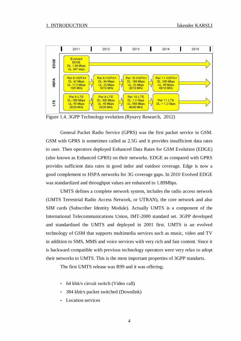
handle their evolving traffics efficiently. Figure 1.4 shows 3GPP technologies
evolutions year by year. Throughput values indicated in the figure are theoritical
values.
1. INTRODUCTION İskender KARSLI
4
Figure 1.4. 3GPP Technology evolution (Rysavy Research, 2012)
General Packet Radio Service (GPRS) was the first packet service in GSM.
GSM with GPRS is sometimes called as 2.5G and it provides insufficient data rates
to user. Then operators deployed Enhanced Data Rates for GSM Evolution (EDGE)
(also known as Enhanced GPRS) on their networks. EDGE as compared with GPRS
provides sufficient data rates in good indor and outdoor coverage. Edge is now a
good complement to HSPA networks for 3G coverage gaps. In 2010 Evolved EDGE
was standardized and throughput values are enhanced to 1.89Mbps.
UMTS defines a complete network system, includes the radio access network
(UMTS Terrestrial Radio Access Network, or UTRAN), the core network and also
SIM cards (Subscriber Identity Module). Actually UMTS is a component of the
International Telecommunications Union, IMT-2000 standard set. 3GPP developed
and standardised the UMTS and deployed in 2001 first. UMTS is an evolved
technology of GSM that supports multimedia services such as music, video and TV
in addition to SMS, MMS and voice services with very rich and fast content. Since it
is backward compatible with previous technology operators were very relax to adopt
their networks to UMTS. This is the most important properties of 3GPP standarts.
The first UMTS release was R99 and it was offering;
• 64 kbit/s circuit switch (Video call)
• 384 kbit/s packet switched (Downlink)
• Location services
1. INTRODUCTION İskender KARSLI
5
• Call services: compatible with Global System for Mobile Communications
(GSM), based on Universal Subscriber Identity Module (USIM)
Then (HSDPA High-Speed Downlink Packet Access) was introduced with
Release 5 which was published in March 2002. HSDPA is an enhanced 3G
communications protocol in the High-Speed Packet Access (HSPA) family, also
named as 3.5G, 3G+ or turbo 3G, which allows networks based on UMTS to have
higher data transfer speeds and capacity. After that Enhanced UL feature was
developed by NOKIA. It was offering 5.76 Mbps in uplink. This feature is
standardized as HSUPA with Release 6 in March 2005.
HSPA + started with 3GPP release 7 and gave 28Mbps. Now it provides 84.4
Mbps in DL ; 23 Mbps with release 9. It reaches these rates by using 64 QAM
modulation, 2x2 MIMO and and dual carrier with 10 Mhz. There is no device yet.
Release 10 was introduced because of growing demand for increased data
rates. Release 10 will use up to 4x5Mhz carriers with 2x2 MIMO and 64 QAM
modulation. It will reach up 168 Mbps.
Release 11 for HSPA provides 8-carrier on the downlink, uplink
enhancements to improve latency, dual-antenna beamforming and MIMO,
DLCELL_Forward Access Channel (FACH) state enhancement for smart phone-type
traffic, four-branch MIMO enhancements and transmissions for HSDPA, 64 QAM in
the uplink, downlink multi-point transmission, and non-contiguous HSDPA carrier
aggregation.
Table 1.1 shows maximum DL data rates associated with the releases. UE
category should be suitable to reach up these rates.
Table 1.1. Max Data Rates and Releases 3GPP Release HSDPA UE Category Modulation MIMO Carrier Max. data rate [Mbit/s] in DLRelease 5 10 16-QAM No 5 Mhz 14Release 7 14 64-QAM No 5 Mhz 21.1Release 7 16 16-QAM 2x2 MIMO 5 Mhz 28Release 7 20 64-QAM 2x2 MIMO 5 Mhz 42.2Release 8 24 64-QAM No Dual-Carrier (10Mhz) 42.2Release 9 28 64-QAM 2x2 MIMO Dual-Carrier (10Mhz) 84.4Release 10 Not Ready 64-QAM 2x2 MIMO Multi-Carrier (20Mhz) 168

1. INTRODUCTION İskender KARSLI
6
Table 1.2 shows required categories to reach up related speeds.
Table 1.2. HSUPA Categories HSUPA Category Max Uplink Speed Examples
Category 1 0.73 Mbit/sCategory 2 1.46 Mbit/sCategory 3 1.46 Mbit/sCategory 4 2.93 Mbit/s Qualcomm 6290
Category 5 2.00 Mbit/s
Nokia: X3-02, X3-01, N8, C7[2], C5[3], C3-01, E52, E72, E55, 6700 Classic, N900, 5630 XpressMusic; BlackBerry: Storm 9500, 9530; HTC: Dream, Passion (Nexus One)[4]; Sony Ericsson C510, Sony Ericsson C903, Sony Ericsson W705, Sony Ericsson T715 , Samsung Wave , Samsung Wave 2
Category 6 5.76 Mbit/s
Nokia CS-15, Option GlobeTrotter Express 441/442, Option iCON 505/505M, Samsung i8910, Apple iPhone 4[5], Huawei, E180/E182E/E1820/E5832/EM770W, Micromax A60, ST-Ericsson M5730, Motorola Atrix 4G(Enabled through software update), Samsung Galaxy S 4G, Sony Ericsson W995,
Category 7 (3GPP Rel7) 11.5 Mbit/s
Category 8 (3GPP Rel9) 11.5 Mbit/s 2 ms, dual cell E-DCH operation, QPSK only, see 3GPP Rel 9 TS 25.306 figure 5.1g
Category 9 (3GPP Rel9) 23 Mbit/s 2 ms, dual cell E-DCH operation, QPSK and 16QAM, see 3GPP Rel 9 TS 25.306 figure 5.1g
Long Term Evolution (LTE) based on OFDM technology is the next step for
UMTS-HSPA network oparetors which are already have GSM technology. It is
needed greater capacity networks and lower costs per bit to meet the future demand
for future mobile broadband. HSPA was the first step and it was continued with
HSPA+. 3GPP started to develope LTE simultaneously and promise higher
throughput. LTE introduces a new radio interface named as E-UTRAN to deliver
higher data rates and fast connection times. Another key renewal is spectral
flexibility. It can be deployed in many frequency bands with minimal changes in
radio equipments. There are also some developments in core network side. LTE core
network arhitecture is named as evolved Packet Core (EPC) that provides easier
connectivity with other 3GPP and 3GPP2 as well as Wi-Fi and fixed line broadband
networks. LTE is an all-IP system throughout the radio access and core network.
LTE is also called as 4G in the market.
While the work towards completion and publication of Rel-8 was ongoing,
planning for content in Release 9 (Rel-9) and Release 10 (Rel-10) began. In addition
to further enhancements to HSPA+, Rel-9 was focused on LTE/EPC enhancements.
Due to the aggressive schedule for Rel-8, it was necessary to limit the LTE/EPC

1. INTRODUCTION İskender KARSLI
7
content of Rel-8 to essential features (namely the functions and procedures to support
LTE/EPC access and interoperation with legacy 3GPP and 3GPP2 radio accesses)
plus a handful of high priority features (such as Single Radio Voice Call Continuity
[SRVCC], generic support for non-3GPP accesses, local breakout and CS fallback).
The aggressive schedule for Rel-8 was driven by the desire for fast time-to-market
LTE solutions without compromising the most critical feature content. 3GPP targeted
a Rel-9 specification that would quickly follow Rel-8 to enhance the initial Rel-8
LTE/EPC specification. At the same time that these Rel-9 enhancements were being
developed, 3GPP recognized the need to develop a solution and specification to be
submitted to the ITU for meeting the IMT-Advanced requirements. Therefore, in
parallel with Rel-9 work, 3GPP worked on a study item called LTE-Advanced,
which defined the bulk of the content for Rel-10, to include significant new
technology enhancements to LTE/EPC for meeting the very aggressive IMT-
Advanced requirements, which were officially defined by the ITU as “4G”
technologies. On October 7, 2009, 3GPP proposed LTE-Advanced at the ITU
Geneva conference as a candidate technology for IMTAdvanced and one year later in
October 2010, LTE-Advanced was approved by ITU-R as having met all the
requirements for IMT-Advanced (final ratification by the ITU occurred in November
2010). (4g Americas, 2011a). Some of the key features of IMT Advanced include:
• Support of wider bandwidth.
• Uplink and downlink enhancements, respectively.
• Support for Relays in the LTE-Advanced network.
• Support of heterogeneous network.
• MBMS enhancements
• SON enhancements.
• Vocoder rate enhancements.
(4g Americas, 2011a)
So LTE release 10 is known as LTE advanced. Key features include carrier
aggregation, multi-antenna enhancements such as enhanced downlink MIMO and

1. INTRODUCTION İskender KARSLI
8
uplink MIMO, relays, enhanced LTE Self Optimizing Network (SON) capability,
eMBMS, Het-net enhancements that include enhanced Inter-Cell Interference
Coordination (eICIC), Local IP Packet Access, and new frequency bands. For HSPA,
includes quad-carrier operation and additional MIMO options. Also includes
femtocell enhancements, optimizations for M2M communications, and local IP
traffic offload.
Release 11 In development, targeted for completion end of 2012. For LTE,
emphasis is on Co-ordinated Multi-Point (CoMP), carrier-aggregation enhancements,
and further enhanced eICIC including devices with interference cancellation. The
release includes further DL and UL MIMO enhancements for LTE. For HSPA,
provides 8-carrier on the downlink, uplink enhancements to improve latency, dual-
antenna beamforming and MIMO, DLCELL_Forward Access Channel (FACH) state
enhancement for smart phone-type traffic, four-branch MIMO enhancements and
transmissions for HSDPA, 64 QAM in the uplink, downlink multi-point
transmission, and non-contiguous HSDPA carrier aggregation.
In our thesis, first 6 sections includes the theory of LTE. It is given
fundamentals of LTE core network (EPC) and also radio access (E-UTRAN) side.
MIMO subject is explained in a separate section. This section also defines materials
and equipments used in thesis. Test equipment and test properties are also explained
in addition to parameters used in test cases in MIMO section. Dual Carrier theory is
also included in this section. During the test, drive tests are carried out for 3 cases.
Each test cases and related properties are given in table 1.3.
Table 1.3. Test Cases and Properties Test Case Technology Release Modulation MIMO Carrier UE Category
Case 1 LTE MIMO Rel-8 64 QAM 2x2 20/20 LTE UE Cat 3Case 2 LTE SIMO Rel-8 64 QAM No 20/20 LTE UE Cat 3Case 3 HSPA + DC Rel-8 64 QAM No 10/10 HSPA UE Cat 24

1. INTRODUCTION İskender KARSLI
9
In test Cases section, signal plots and graphs are given for each test scenario
and also it is included some comments about the figures. There are two main
objectives of our thesis.
• The first objective in this thesis is to investigate the importance of MIMO
technique which is a key property for LTE networks. To do that 2 drive
tests are carried out (Test Case1 and 2).
• The second objective in this thesis is to investigate the main factor of
throughput is related with technology or not. By invastigating this, test
results of case 1 and case 2 are compared with the result of another test
scenario (Test Case 3) which are taken from a real HSPA network that is
implemented with one the last release of a HSPA system.
Results and Analysis section includes summaries, comments and advices
about the usage of MIMO and SIMO.

1. INTRODUCTION İskender KARSLI
10

2. NETWORK ARCHITECTURE AND ENTITIES İskender KARSLI
11
2. NETWORK ARCHITECTURE AND ENTITIES
LTE has been desinged as latter technology of 3G HSPA. It consists of an
evolved radio access system which is named as Evolved UMTS Terrestrial Radio
Access Network (E-UTRAN) and “System Architecture Evolution” SAE that
includes Evolved Packet Core (EPC) network. Together E-UTRAN and SAE
compose the Evolved Packet System (EPS). In this thesis, the terms LTE and E-
UTRAN will both be used to refer to the evolved air interface and radio access
network based on OFDMA, while the terms SAE and EPC will both be used to refer
to the evolved flatter-IP core network. The main objectives of the SAE is to evolve
the 3G access technologies and their supporting GPRS core network by creating a
simplified All-IP architecture to provide support for multiple radio accesses,
including mobility between various access networks, both 3GPP and Non-3GPP
standardized technologies. (4G Americas, 2011b)
Main entities in EPS are;
• Evolved NodeB (eNB)
• Mobility Management Entity (MME)
• Serving Gateway (S-GW)
• PDN Gateway (P-GW)
2. NETWORK ARCHITECTURE AND ENTITIES İskender KARSLI
12
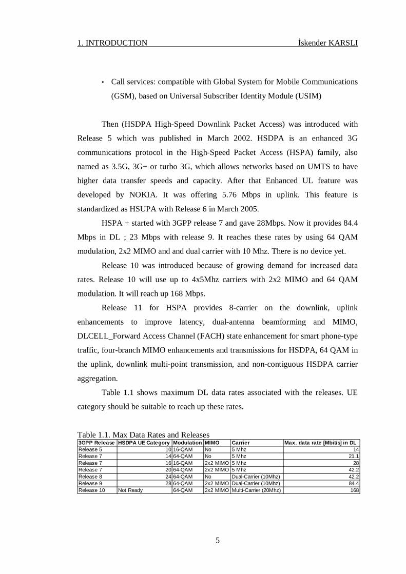
Figure 2.1. EPS network architecture and ınterfaces
P-GW, MME and S-GW are EPC network elements on the other hand eNB’s
are E-UTRAN network elements.
2.1. Evolved NodeB (eNB)
eNB is the base statiton system of LTE. It is responsible to support user plane
and control plane. eNB's are connected to each other with fully meshed configuration
with an interface of X2. The main functions of eNB are;
• Transferring user plane and control plane datas between Uu and S1
interfaces.
• Radio channel chippering and dechippering function over air interface
against unauthorized accesses.
• Scheduling process and rate adaptation
• Radio measurements that are used for handover and calculations to reach
target QoS required.

2. NETWORK ARCHITECTURE AND ENTITIES İskender KARSLI
13
• Paging for UE’s in idle state.
• Inter cell interference decreasing.
• Connection setup and release.
• Load balance in order to minimize drop risks because of congestion. It
may leads to cell reselection or handover.
• Distribution of NAS messages.
• Selection of MME/S-GW for UE.
• Synchronization between other nodes in the network.
2.2. Mobility Management Entity (MME)
Mobility Management Entity (MME) is a control node that provides mobility
management and session management via Non-Access Stratum (NAS) protocol.
NAS is the protocol between MME and UE and responsible for EPS bearer
management, authentication, security control, idle mode mobility/paging handling.
MME is signalling only element in EPC system means no IP data packets pass
through the MME. It provides, signalling loads and data loads not effecting each
other and then they can increase independently. The main functions of MME are;
• Idle Mode Management including distrubution of paging messages.
• Authentication and security control.
• Bearer manegement including bearer establishment.
• Intra LTE Handover
• NAS signalling.
• P-GW/S-GW selection.
• Mobilty to other 3GPP or non 3GPP networks.

2. NETWORK ARCHITECTURE AND ENTITIES İskender KARSLI
14
2.3. Serving Gateway (S-GW)
Serving Gateway (S-GW) is responsible for transferring user data packets
coming from eNB interface through the P-GW. S-GW is instructed by MME and
work as a mobility base for data bearers when the UE moves between eNB’S. The
main functions of MME are;
• Encryption of user data streams.
• Termination of packets for paging resons.
• Data path responsibility.
2.4. PDN Gateway (P-GW)
PDN Gateway (P-GW) provides connectivity to external data networks such
as internet or other non 3GPP networks i.e. WIMAX or CDMA2000. It also allocates
IP adress for UE’s.

3. E-UTRAN PROTOCOL ARCHITECTURE İskender KARSLI
15
3. E-UTRAN PROTOCOL ARCHITECTURE
Each user IP packet is encapsulated with a spesific protocol across interfaces
and tunnelled between UE and P-GW. Tunneling is a transferring method and it is
implemented by establishing an infrasturucture between networks or interfaces.
Instead of sending a frame with its created form in source, the frame is encapsulated
in an additional header using tunnelling method. A 3GPP-specific tunnelling protocol
called the GPRS Tunnelling Protocol (GTP) is used over the EPC network interfaces,
S1 and S5/S8.
In this thesis only Uu interface protocol layer is examined since the scope of
this thesis is related with E-UTRAN side of the LTE system. Uu interface protocol
layer structure has been shown in Figure3.1. As previously mentioned, LTE has been
designed as latter technology of HSPA system. With this idea eNb’s have same
functionality of NodeB’s and also support implemented protocols in RNC’s. This
leads eNb’s to have a role of admission control and radio resource management
beside routine roles. It works like RNC’s in HSPA. It makes LTE more beneficial
than HSPA. Because processor load of RNC is distrubuted to a lot of eNB's and
latency is minimized. Figure 3.1 shows the Uu interface protocol layers.
Figure 3.1. User Plane and Control Plane Protocol Layers
User plane protocols implement the bearer services to carry user data. Control
plane protocols additionally perform controlling of bearers and connections. UE and
eNB both consist of user plane and control plane protocol layers. User plane
protocols include PDCP, RLC, MAC, PHY protocol layers. Control plane protocols

3. E-UTRAN PROTOCOL ARCHITECTURE İskender KARSLI
16
also include NAS and RRC protocols in addition to user plane. NAS in UE
communicates with NAS in MME via eNB and RRC in UE communicates directly
with RRC in MME.
3.1. Protocol Layers
It will be more clear when the protocol layers are examined subsequently.
Figure 3.2 shows processes of an IP packet carried with a SAE bearer in each
protocol layer.
Figure 3.2. LTE Protocol Architecture and Functions Downlink (Dahlman, Parkvall,
Sköld and Beming, 2008 )

3. E-UTRAN PROTOCOL ARCHITECTURE İskender KARSLI
17
PDCP (Packet Data Convergence Protocol): PDCP layer performs IP header
compression to prevent unnecessary overhead in the payload. The IP header
compression mechanism is Robust Header Compression (ROHC) which is also used
in WCDMA systems. This layer is also responsible for ciphering and integrity of
transmitted data. In the reciever part, Header decompression and dechippering
processes are carried out. There is one PDCP entity per SAE beaerer in UE side.
RLC (Radio Link Control): RLC is reponsible for segmentation/concetenation of
header compressed IP packets, RLC retransmission and in sequence delivery of
messages to higher layers. RLC offers services to PDCP in form of radio bearer.
There is one RLC entity per radio bearer in UE side. Generally data packets coming
from/to a higher layer is called as SDU and corresponging data packets coming
from/to lower layer is called as PDU. RLC layer selects certain amount of data
according the scheduler decision from RLC SDU buffer and these SDUs are
segmented to create PDUs. For high data rates relatively large PDUs with smaller
RLC header payloads are created, for low data rates smaller PDUs with large
payloads are created. In LTE RLC PDU sizes change dynamically. Since scheduling
process, rate adaptation and RLC layer is located in eNodeB, PDU sizes are
dynamically adjusted easly.
Figure 3.3. RLC Segmentation and Concetenation (Dahlman, Parkvall, Sköld and
Beming, 2008)
Figure 3.3 shows the process of segmentation/concetenation. In each RLC
PDU, an RLC Header payload is included. This header consists of a sequence

3. E-UTRAN PROTOCOL ARCHITECTURE İskender KARSLI
18
number for in-sequence delivery of the packets and retransmission cases. RLC
retransmission is known as automatic repeate request (ARQ). ARQ mechanism
provides error-free delivery of data packets to higher layers. This retransmission
algorithm is carrried out by the RLC layers in both transmitter and reciever side. By
monitoring the sequence number of recieved RLC PDU in reciever side, missing
PDUs are detected. Then the missing PDU is requested transmitter side. The ARQ
retransmisson occurs in two cases. First case occurs when a missing RLC PDU is
detected. Second case occurs when HARQ process reaches maximum transmission
numbers of a transport block. In this case RLC starts RLC segmentation process
again.
MAC (Medium Access Control): MAC layer configures Hybrid-ARQ
retransmissions, uplink/downlink scheduling and logical channels multiplexing.
Main difference between UL and DL is priority handling between Ues and priority
handling of logical channels. The scheduling functionality is carried out by eNBs.
There is one MAC entity per cell for both uplink and downlink. The HARQ is
present in both UE and eNB. MAC offers services to RLC in form of logical
channels. In HSPA systems UE monitors sheduling information from all cells which
are in soft handover. The non-serving cells can request all its non-served users to
lower their data rates to control interference level in environment. In LTE system this
operation is different. LTE defines only one serving cell which is only responsible
entity for scheduling and HARQ operation. MAC layer offer services to physical
layer in form of transport channels. A transport channel is defined by how and with
what characteristics the information will be transmitted over radio interface. Data in
transport channels are carried by transport blocks. In each Transmission time interval
(TTI) one transport block is trasfered over radio interface. If it is used spatial
multiplexing (MIMO) two transport blocks are transfered in each TTI over radio
interface. Associated with each transport block is Transport format (TF). TF specifies
how the transport block is transmitted over radio interface. TF includes information
about transport block size, modulation scheme an antenna mapping. By changing the
transport format MAC layer achieve different data rates. That’s why data rate control
is also known as transport-format selection.

3. E-UTRAN PROTOCOL ARCHITECTURE İskender KARSLI
19
Main function of the LTE radio access is shared channels assignments to each
user. In LTE time and frequency resources are dynamically shared between users.
Scheduling is the main function of MAC layer and controls the uplink and downlink
resources. eNodeB makes dynamic scheduling and sends scheduling informations in
each 1ms TTI to certain amount of terminals.
HARQ is a method that is used to eliminate transmission errors. Transport
blocks which are not correctly recieved are buffered and then they are corrected by
requesting retransmission. There are two HARQ scheme avaiable. First one is
proposed by Chase. In chase method initial transmission and retransmission are
identical. The reciever always combine failed block and retransmission and it
corrects the errored block. The other scheme is named as IR (Incremental
Redundancy). In the IR scheme, progressive parity packets are sent in each
subsequent transmission of packet. Reciever combines all these low code rate
packets to correct errored blocks. However IR can provide better performance, it
needs UE complexity because of the buffering. In LTE both IR and Chase schemes
are used.
Physical Layer: Physical Layer configures coding/decoding, modulation/
demodulation, multiple antenna mapping etc. It offers services to MAC layer in form
of transport channels. It provides mapping of transport channels onto physical
channels. The Physical layer is responsible for reporting of radio channel
measurements to higher layers and MIMO antenna signals processing, transmit
diversity, and beam forming. Both FDD (Frequency Division Duplex) and TDD
(Time Division Duplex) are supported on physical layer in LTE. FDD and TDD use
same framing structure. This frame has a duration of 10ms and consists of 20 time
slots. 2 adjacent time slots form a sub-frame and it spans to 1 ms ( 0.5ms*2).
LTE downlik and uplink pyhsical channels except broadcast channel use
QPSK, 16QAM, or 64QAM. Broadcast channel uses only QPSK. As a result LTE
physical layer supports both FDDand TDD mode.

3. E-UTRAN PROTOCOL ARCHITECTURE İskender KARSLI
20
• FDD: downlink and uplink are identified with two different frequency
bands
• TDD: downlink and uplink signals are transmitted in different time slots
Figure 3.4. FDD and TDD Modes
RRC (Radio Resource Control): RRC protocol is used for communication between
UE and eNb and responsible for all signalling between UE and network. It transfers
broadcasting system information message, paging and establishing RRC connection
with UE to alllocate temporary identifiers (RA-RNTI). RRC layer is also responsible
for integrity of RRC messages. UE measurement and reporting, intra-LTE handover,
UE cell re/selection, and context transfer are handled by the RRC layer. RRC also
support MBMS services.
NAS (Nonaccess Stratum): NAS protocol layer is used for network entry(Attach),
authentication, data bearers setup and release, mobility management. NAS signalling
security is provided by chippering and NAS messages are transfered from/to UE by
RRC layer.
In previous chapters it is mentioned in detail that UEs in LTE undertake some
key roles like admission and resource management which are previously made by
RNCs in 3G. By doing that latency target in LTE is provided. Figure 3.5 shows a
clear representation of functions of UMTS and EPS sytems in DL user plane.

3. E-UTRAN PROTOCOL ARCHITECTURE İskender KARSLI
21
Figure 3.5. Differences between UMTS and EPS in downlink user plane handling
(Lescuyer and Lucidarme, 2008)
3.2. Terminal States
In LTE, terminal can be in two different states as shown in figure 1.6.
Terminal is in RRC_CONNECTED state while in active mode. In this state, terminal
is connected to a cell within a network. One or more IP adresses have been assigned
to the terminal in addition to identifier which is called Cell Radio-Network
Temporary Identifier (C-RNTI). C-RNTI is used for signalling pruposes between the
terminal and the network. RRC_CONNECTED has two substates IN_SYNC and
OUT_OF_SYNC which depend on the terminal is uplink synchronized or not. Since
LTE use FDMA/TDMA in uplink direction UL synchronization is very important for
mobile terminals which try to transmit their datas aproximately at same time. To
adjust the synchronization, eNodeB measures arrival time of the trasnmission of each
3. E-UTRAN PROTOCOL ARCHITECTURE İskender KARSLI
22
mobile terminal and sends timing-correction message in downlink direction. Unless
UL synchronization is not provided L1/L2 signalling can not be possible. If no
uplink transmission occurs in a specified time, UL is declared as non-syncronized. In
this case mobile starts the random access procedure to restore the Ul synchronization.
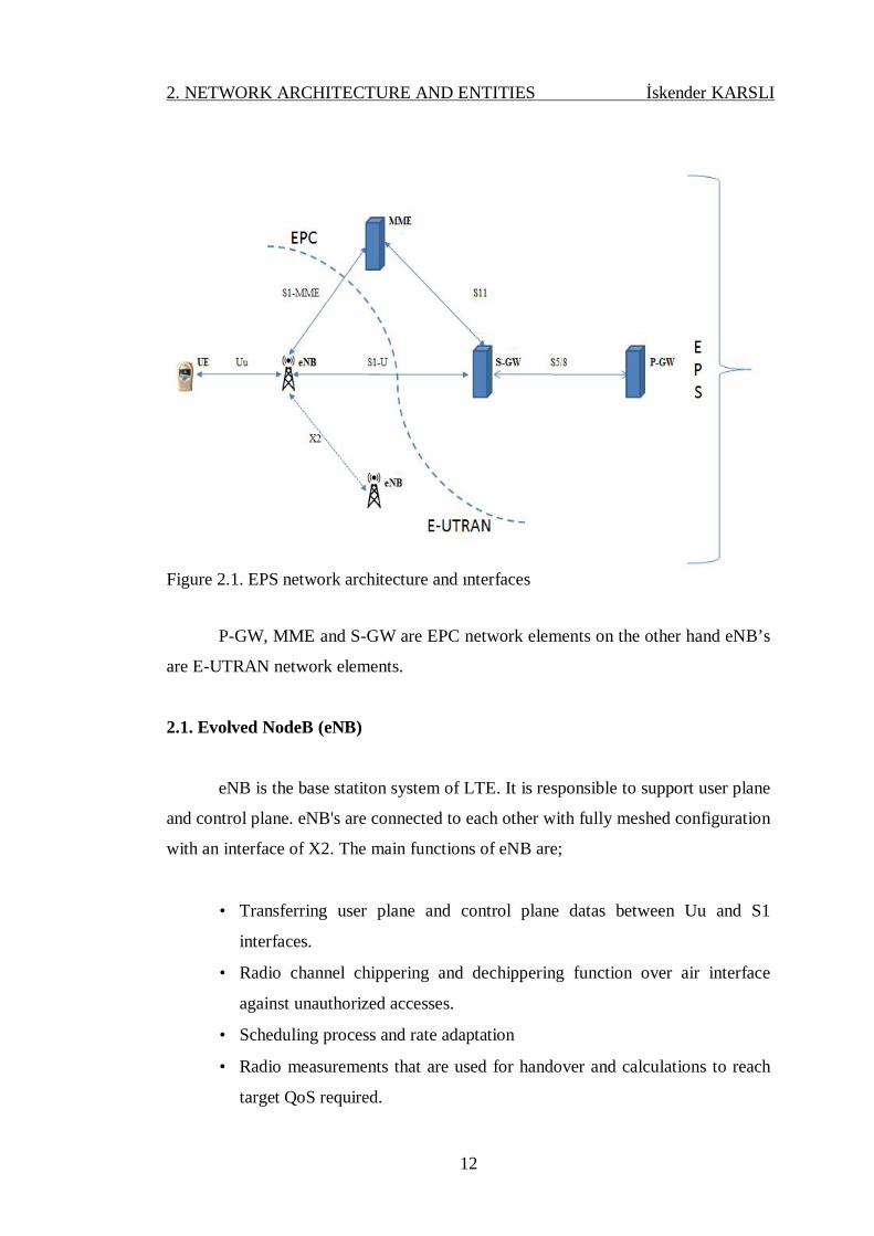
Figure 3.6. LTE States
In RRC idle state the terminal sleeps most of the and has very low activity to
minimize battery consumption. There is no UL syncronization since the only UL
taransmission activity is random access. In the downlink mobile listens paging
channel periodically. The mobile keeps its IP adresse in order to move
RRC_CONNENCTED state when required.
3.3. LTE Data Flow
IP packets are transfered from S-GW through eNB’s in form of SAE bearers.
As explained previously IP header compresssion and chippering is applied these
beareres and then a PDCP header is added. This header carries information about
chippering for UE. RLC layer performs segmentation/concetanation of RLC SDU’s
and adds RLC header which is used for in sequence delivery of RLC PDUs. In
sequence delivery of RLC PDUs are used for ARQ retransmission in receive part. As
previously explained RLC PDU size adjusted according to the scheduler decision in
MAC layer. And then RLC PDUs are transfered to the MAC layer. Certain number

3. E-UTRAN PROTOCOL ARCHITECTURE İskender KARSLI
23
of RLC PDUs are put in a MAC SDU and a MAC header is added to form a
transport block. Transport block size also depends on scheduler algorithm. It can be
said that Transport block size and RLC PDU size are depended on scheduler
algorithm. In physical layer CRC header is attaced to the transport block for error
detection. Physical layer is responsible for coding, modulation and transmission of
signal to air interface.
Figure 3.7. LTE Data Flow (Dahlman, Parkvall, Sköld and Beming, 2008 )
3.4. Quality of Service (Qos)
Each applications such as VoIP, streaming, video telephony, web browsing
need specific quality of service (QoS). Therefore EPS system selects different QoS
data flows for each service. These QoS flows are called as EPS bearers and
established between UE and P-GW. Radio bearers transport the packets of an EPS
bearers between UE and eNB. Lets consider someone makes web browsing with his
UE. P-GW when recieving an IP packet from internet will classify the packet and
then select a definite EPS bearer to transport the packet from P-GW to eNB and then
eNB will select an appropriate radio bearer to transport EPS bearer to UE. In another
example consider a UE who makes VoIP while making web browsing. As we know

3. E-UTRAN PROTOCOL ARCHITECTURE İskender KARSLI
24
VoIP is more delay sensitive service than web browsing and needs more strict QoS
in terms of delay. Therefore each IP packet is associated with a spesific EPS bearer
so it lets the network can prioritize traffic.
Figure 3.8. EPS Bearer Architecture

4. LTE CHANNEL STRUCTURE İskender KARSLI
25
4. LTE CHANNEL STRUCTURE
Figure 4.1. LTE Protocol Layers and Channels
Layer1 includes physical layer which consists of mixture of technologies. It
uses OFDMA as access technology, QAM as modulation scheme and MIMO
tecnique to achieve high speeds. Layer2 includes 3 sublayers which are MAC, RLC
and PDCP. Layer3 includes RRC and NAS layers. MAC layer is connected to RLC
with logical channels while connected to PHY layer with transport channels. MAC
layer sends and receives the MAC PDUs to/from the physical layer via transport
channels. The connection to RLC layer is provided by logical channels by means of
RLC Service Data Units (SDUs). Logical channels are identified by information
carried by them. Transport channels are identifed according to their transmission
characteristics. Similarly, physical channels are characterized by their configuration
for data protection. Fig. 4.1 shows the LTE mapping structure of channels for uplink
and downlink.

4. LTE CHANNEL STRUCTURE İskender KARSLI
26
• The Logical Channels – What it is transmitted
• The Transport Channels – How it is transmitted
• The Physical Channels
4.1. Logical Channels
MAC layer offers services to RLC layer in forms of logical channels. Two
types of logical channels are available. Control and trafic channels. The control
channels carry control-plane information, while traffic channels carry user-plane
information.
Logical control channels are;
• BCCH: If there is no data transmission, mobile devices are in idle state. In
idle state mobile devices listen Broadcast Control Channel (BCCH) which
is used by the network to transmit system control information. The system
informations include the configuration of common channels, operator
related informations and parameters to access the cell and the network.
• PCCH: Paging Control Channel is used for transmitting paging
information. This channel is used when the system has no knowlege about
the UE’s location.
• CCCH: Common Control Channel is used by UE when UE has no RRC
connection. This channel is used in very early phase of connection
establishment. And it is used for transmission of control informations
together with random access.
• DCCH: Dedicated Control Channel is a point-to-point bidirectional
channel used for UEs that have an RRC connection. It includes RRC and
NAS signalling. This channel is used for transmission of control
information in UL and DL.
• MCCH: Multicast Control Channel is used for transmittting MBMS
control information from eNB to one or multiple Ues. The MCCH is used
by only those UEs receiving MBMS.

4. LTE CHANNEL STRUCTURE İskender KARSLI
27
Figure 4.2. LTE Downlink and uplink channels
Logical traffic channels are;
• DTCH: Dedicated Traffic Channel is a point-to-point bidirectional channel
dedicated to a single UE for the transmission of user trafic data. It is used
between on terminal and the network.
• MTCH: Multicast Traffic Channel is a point-to-multipoint channel for
transmitting user traffic data from the network to the UEs. It is used
between one or several terminals and the network.
4.2. Transport Channels
Transport channels pass data to/from higher layers and configures PHY layer.
Transport channels describe how the data are transferred over the radio interface. It
describes the type of channel coding, CRC protection or interleaving and data rates
for protection of the data against transmission errors. Transport channels are
classified in 2 groups which are downlink and uplink transport channels.
Transport channels for downlink are;
• BCH: BCCH channel is mapped to BCH in transport channels and this
channel is the first channel recieved by UE after sychronization. BCH is
transmitted through entire cell area with a fixed transport format.

4. LTE CHANNEL STRUCTURE İskender KARSLI
28
• DL-SCH: Logical channels BCCH, CCCH, DCCH, DTCH, MTCH are
mapped to Downlink Shared Channel in transport channels. DL-SCH is
used for HARQ, adaptive modulation/coding, power control, semi-
static/dynamic resource allocation, DRX, MBMS transmission and
multiantenna technologies. As a result it is used to transport user control
and trafic data. Another function of DL-SCH is transmission of the parts of
BCCH which is not mapped to the BCCH for single cell MBMS services.
• PCH: PCCH is mapped to PCH in transport channels. PCH supports
discontionious reception called DRX which is used for UE power saving.
It is broadcasted over cell erea. It is associated to the BCH.
• MCH: Multicast Channel supports Multicast Broadcast -Single Frequency
Network (MB-SFN) combining of MBMS transmission from different
cells.
Transport channels for uplink are;
• UL-SCH: Uplink Shared Channel supports HARQ, adaptive
modulation/coding, power control, semi-static/dynamic resource
allocation. It is uplink equivalent of DL-SCH.
• RACH: Random Access Channel is used by terminals and includes a
limited control information. RACH is used in a case of RRC state change
and at beginning of connection establishment.
4.3. Physical Channels
Physical channels are actual implementation of transport channels over radio
interface.
LTE downlink physical channels are as follows:
• PDSCH: Physical Downlink Shared Channel is used for data transport. It
carries high data rates with QPSK, 16QAM, and 64QAM modulation with
1/3 turbo coding and spatial multiplexing. As a result PDSCH carries user
data packets.

4. LTE CHANNEL STRUCTURE İskender KARSLI
29
• PBCH: As previously explained logical BCCH is used to transmit the
system information of transmitter. The informations distrubuted by the
BCCH channel are mapped to BCH in transport channels and then PBCH
in physical channels.
• PMCH: The multicast channel MCH is mapped to physical multicast
channel (PMCH). It transfers Multicast/Broadcast information.
• PCFICH: The PCFICH is transmitted every subframe and carries
information on the number of OFDM symbols used for PDCCH.
• PDCCH: The PDCCH is used to inform the UEs about the resource
allocation of PCH and DL-SCH as well as modulation, coding and hybrid
ARQ information related to DL-SCH. A maximum of three or four OFDM
symbols can be used for PDCCH.
• PHICH: Physical HARQ indicator channel is used to carry HARQ
Ack/Nack messages.
LTE uplink physical channels are the following:
• PUSCH: Physical Uplink Shared Channel is uplink equivalent of PDSCH
and transfers user data packets with QPSK, 16QAM, or 64QAM
modulation.
• P-RACH: RACH is mapped to P-RACH in uplink physical channel and
carries the random access preamble.

4. LTE CHANNEL STRUCTURE İskender KARSLI
30

5. ORTHOGONAL FREQUENCY DIVISION MULTIPLEXING (OFDM) İskender KARSLI
31
5. ORTHOGONAL FREQUENCY DIVISION MULTIPLEXING (OFDM)
LTE multiple access is based on Single-carrier FDMA (SC-FDMA) in uplink
direction and OFDMA in downlink direction. OFDMA has been also adopted
WIMAX downlink transmission scheme. OFDM is a type of multi carrier
transmission used in high data rate communication systems. Before explaning the
OFDM, it will be useful to remember the difference of modulation and multiplexing
briefly.
• Modulation is a method for carrying an amounth of informations by
changing carrrier phase, amplitude or combination.
• Multiplexing is a method for sharing a bandwith to multiple user.
OFDM is a combination of modulation and multiplexing. In OFDM main
signal is split into subchannels which are orthogonal to each other. After that, each
subchannel is modulated and then re-multiplexed to create OFDM carrier. OFDM is
a special form Frequency Division Multiplexing (FDM). Figure 5.1 shows the
difference between FDM and OFDM. There are two possibilities to carry our cargo.
One is to hire a big truck and the other one is to split our cargo to smaller trucks. In
both cases we carry same amount of cargo but in the OFDM truncking, ¼ of the
cargo is lost in case of an accident. Consider each smaller trucks as subcarriers in
OFDM. These subcarriers must be othogonal.
Figure 5.1. All cargo on one truck vs splitting the shipment into more than one
(Langton, S.,2004)
In FDM total signal bandwidth is divided into nonoverlapping frequency
subchannels. Each subchannel is modulated with a symbol an then multiplexed.
5. ORTHOGONAL FREQUENCY DIVISION MULTIPLEXING (OFDM) İskender KARSLI
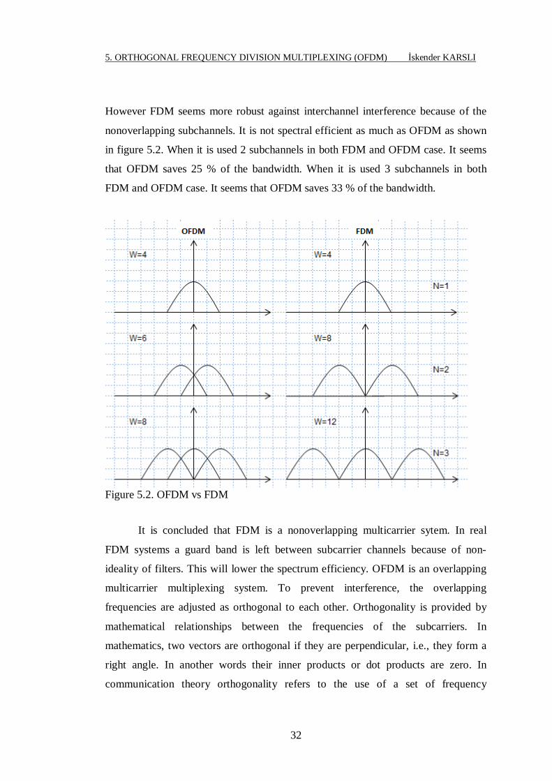
32
However FDM seems more robust against interchannel interference because of the
nonoverlapping subchannels. It is not spectral efficient as much as OFDM as shown
in figure 5.2. When it is used 2 subchannels in both FDM and OFDM case. It seems
that OFDM saves 25 % of the bandwidth. When it is used 3 subchannels in both
FDM and OFDM case. It seems that OFDM saves 33 % of the bandwidth.
Figure 5.2. OFDM vs FDM
It is concluded that FDM is a nonoverlapping multicarrier sytem. In real
FDM systems a guard band is left between subcarrier channels because of non-
ideality of filters. This will lower the spectrum efficiency. OFDM is an overlapping
multicarrier multiplexing system. To prevent interference, the overlapping
frequencies are adjusted as orthogonal to each other. Orthogonality is provided by
mathematical relationships between the frequencies of the subcarriers. In
mathematics, two vectors are orthogonal if they are perpendicular, i.e., they form a
right angle. In another words their inner products or dot products are zero. In
communication theory orthogonality refers to the use of a set of frequency

5. ORTHOGONAL FREQUENCY DIVISION MULTIPLEXING (OFDM) İskender KARSLI
33
multiplexed signals with the exact minimum frequency spacing needed to make them
orthogonal so that they do not interfere with each other. The main principle of
OFDM is dividing the spectrum into narrow orthogonal sub channels called
subcarriers and transmit information parallely in lower data rates.
An OFDM subcarrier is actually a sinc-squared function. Figure 5.3 shows
the time domain and frequency domain representation of an OFDM subcarrier.
Figure 5.3. Time domain and frequency domain representation of an OFDM
subcarrier. (Dahlman, Parkvall, Sköld and Beming, 2008)
Each subcarrier spacing is equal to =1/T where T is per-subcarrier
modulation–symbol time as shown in figure 5.4. The subcarrier spacing is thus equal
to the per-subcarrier modulation rate 1/ T.
Figure 5.4. OFDM Subcarrier spacing. (Dahlman, Parkvall, Sköld and Beming,
2008)
5. ORTHOGONAL FREQUENCY DIVISION MULTIPLEXING (OFDM) İskender KARSLI
34
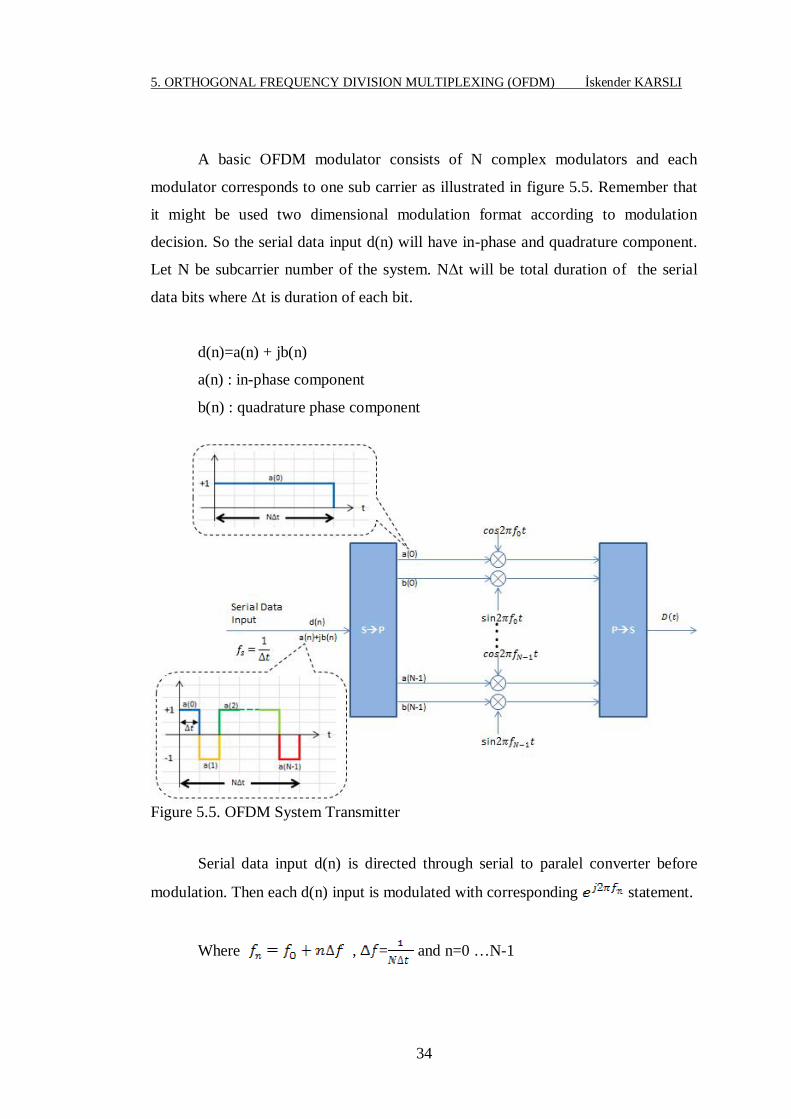
A basic OFDM modulator consists of N complex modulators and each
modulator corresponds to one sub carrier as illustrated in figure 5.5. Remember that
it might be used two dimensional modulation format according to modulation
decision. So the serial data input d(n) will have in-phase and quadrature component.
Let N be subcarrier number of the system. NΔt will be total duration of the serial
data bits where Δt is duration of each bit.
d(n)=a(n) + jb(n)
a(n) : in-phase component
b(n) : quadrature phase component
Figure 5.5. OFDM System Transmitter
Serial data input d(n) is directed through serial to paralel converter before
modulation. Then each d(n) input is modulated with corresponding statement.
Where , = and n=0 …N-1
5. ORTHOGONAL FREQUENCY DIVISION MULTIPLEXING (OFDM) İskender KARSLI
35
Note that serial input bitrate is decreased to lower bit rates after S/P
conversion. Consider a serial system in which 1 bit is transfered in 1 second. So bit
rate will be 1 bits/sec. If it was transfered with a 4 subcarriers parallel system like our
example, what would be the answer? Since it is transfered 4 bits in 1 second, the bit
rate will 0.25 bits/sec. This is the main idea of the OFDM as explained before.
Additionally since the signalling interval is increased to , this will make the
system more stable against to channel delays.
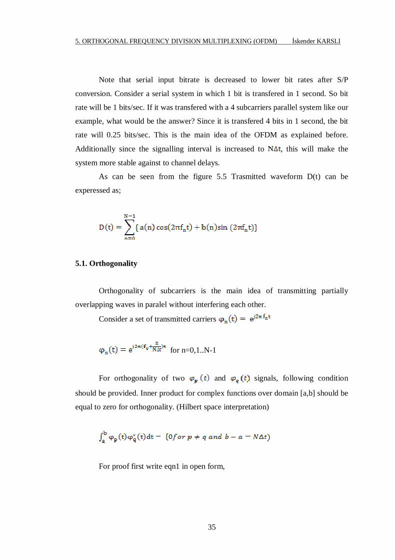
As can be seen from the figure 5.5 Trasmitted waveform D(t) can be
experessed as;
5.1. Orthogonality
Orthogonality of subcarriers is the main idea of transmitting partially
overlapping waves in paralel without interfering each other.
Consider a set of transmitted carriers
for n=0,1..N-1
For orthogonality of two and signals, following condition
should be provided. Inner product for complex functions over domain [a,b] should be
equal to zero for orthogonality. (Hilbert space interpretation)
For proof first write eqn1 in open form,

5. ORTHOGONAL FREQUENCY DIVISION MULTIPLEXING (OFDM) İskender KARSLI
36
=
=
=
=
=
We know that ,
=
If we take the expression in the paranthesis. And since the angle values are
multiples of sine term will be zero and cosine term will be equal to 1. Then
orthogonality condititon is proved.
5.2. OFDM With IFFT/FFT
As shown from the figure1.14 each serial modulation input is multipled by a
complex modulator and last all subcarriers are put in a summation. It is very complex
structure and difficult to implement. There is a more efficient way called Inverse
Fourrier Transform (IFFT) algorithm that eliminates the usage of a lot of complex

5. ORTHOGONAL FREQUENCY DIVISION MULTIPLEXING (OFDM) İskender KARSLI
37
modulators. IFFT provides a fast way to create an OFDM symbol within duration T.
In general an OFDM subcarrier can be represented as;
where complex valued modulation symbols. Since there are N subcarriers in an
OFDM signal. Total complex signal can be written as;
Where and lets assume for this case. Then
If we sample with a sampling frequency which is a multiple
of subcarrier spacing. The multiple should be selected so that the sampling
theorem is sufficiently full filled. Since is bandwith of the OFDM signal,
should be greater than value.
and then equation becomes for sampled
OFDM signal ;
Since .The eqn becomes,
5. ORTHOGONAL FREQUENCY DIVISION MULTIPLEXING (OFDM) İskender KARSLI
38
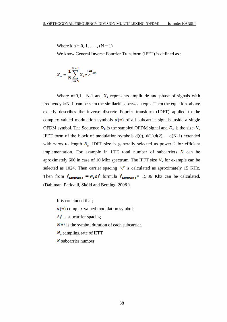
Where k,n = 0, 1, . . . , (N − 1)
We know General Inverse Fourrier Transform (IFFT) is defined as ;
Where n=0,1....N-1 and represents amplitude and phase of signals with
frequency k/N. It can be seen the similarities between eqns. Then the equation above
exactly describes the inverse discrete Fourier transform (IDFT) applied to the
complex valued modulation symbols of all subcarrier signals inside a single
OFDM symbol. The Sequence is the sampled OFDM signal and is the size-
IFFT form of the block of modulation symbols d(0), d(1),d(2) ... d(N-1) extended
with zeros to length . IDFT size is generally selected as power 2 for efficient
implementation. For example in LTE total number of subcarriers can be
aproximately 600 in case of 10 Mhz spectrum. The IFFT size for example can be
selected as 1024. Then carrier spacing is calculated as aproximately 15 KHz.
Then from formula = 15.36 Khz can be calculated.
(Dahlman, Parkvall, Sköld and Beming, 2008 )
It is concluded that;
complex valued modulation symbols
is subcarrier spacing
is the symbol duration of each subcarrier.
sampling rate of IFFT
subcarrier number

5. ORTHOGONAL FREQUENCY DIVISION MULTIPLEXING (OFDM) İskender KARSLI
39
Figure 5.6. OFDM System Transmitter with IFFT (Dahlman, Parkvall, Sköld and
Beming, 2008)
Similar to OFDM modulation, FFT processing is used for OFDM
demodulation. Recieved signal is sampled with a sampling rate
and size- FFT is used as shown in the Figure 5.7.
Figure 5.7. OFDM System Reciever with FFT (Dahlman, Parkvall, Sköld and
Beming, 2008)
5.3. Cyclic Prefix (CP) Insertion
In mobile communication receiver takes transmitted signals through different
paths, some arrives directly, some arrives after a multiple of consequtive reflections
from obstacles. This is the result of time dispersive characteristics of air interface.
Figure 5.8 shows an axample of multipath transmission of an OFDM signal. First
path is directly recieved and the other one represents the reflected path which is

5. ORTHOGONAL FREQUENCY DIVISION MULTIPLEXING (OFDM) İskender KARSLI
40
delayed by . At reciever two paths are recieved and demodulation process is applied
in correlation interval of . Delayed OFDM signal D(t-1) will cause inter symbol
interference (ISI) on D(t). Generally ISI can be defined as the effect of a delayed
version OFDM signal onto an adjacent OFDM signal because of the multipath
transmission.
Figure 5.8. Multipath delay of an OFDM signal and ISI (Dahlman, Parkvall, Sköld
and Beming, 2008 )
One of the most important properties of the OFDM system is robustness of
the signals against multipath delays. Actually the usage of long symbol period time
enhances the ISI problem but besides to eliminate ISI and to improve the robustness
against the multipath delay spread a guard period GP is inserted between successive
OFDM signals.
Figure 5.9. Guard Period Usage to eliminate ISI

5. ORTHOGONAL FREQUENCY DIVISION MULTIPLEXING (OFDM) İskender KARSLI
41
GP eliminates the ISI as can be seen from the figure1.18. However OFDM
signal D(t) is recieved exactly at correlation time interval we still have a possibility
of intercarrier interference (ICI). Generally ICI can be defined as the loss of the
orthogonality of subcarriers. Orthogonality loss is mostly due to the multipath
dispersion of signals. If an OFDM signal is uncorrupted, it can be easly demodulated
without any interference between subcarriers. Demodulator knows that in an OFDM
symbol, which has a period of , there are N subcarriers. Demodulation
occurs for each OFDM symbol in this correlation time interval of . In case of a time
dispersive channel subcarrier orthogonality might be lost. To understand the
orthogonality we should note that each OFDM symbol D(t-1), D(t), D(t+1) consists
of an integer number of periods of complex exponentials, which is multiple of each
other, during demodulator integration interval . The effect of this is illustrated in
Figure 5.10, where subcarrier 1 is aligned to the symbol integration boundary,
whereas subcarrier 2 is delayed. In this case, the receiver will encounter interference
because the number of cycles for the FFT duration is not an exact multiple of the
cycles of subcarrier 2. Fortunately, the ICI can be mitigated with intelligent
exploitation of the guard period, which is required to combat the ISI.
Figure 5.10. Effect of multipath on the ICI (Jha and Prasad, 2007)
Cyclic prefix (CP) is inserted to the begining of the OFDM signal to
eliminate ICI problem. Last part of the signal is copied to the begining of the signal.
Last few subcarriers are added to the begining of the signal within a duration of the

5. ORTHOGONAL FREQUENCY DIVISION MULTIPLEXING (OFDM) İskender KARSLI
42
guard period. If we go back to the figure 5.9 since we put the end of the signal to the
begining. The signal will be correctly demodulated in FFT interval.
Figure 5.11. CP insertion to eliminate ICI
As a result in case of time dispersive channel inter-symbol interference (ISI)
and inter-carrier interfence (ICI) occur.

6. MIMO (MULTIPLE INPUT MULTIPLE OUTPUT) İskender KARSLI
43
6. MIMO (MULTIPLE INPUT MULTIPLE OUTPUT)
Multi-antenna techniques can be used to improve system performance,
including improved system capacity (more users per cell) and improved coverage
(larger cell coverage ), as well as improved per-user data rates. Multiple antenna
techniques are the integrated part of LTE specifications because some requirements
such as user peak data rates cannot be achieved without the utilization of multiple
antenna schemes. The radio link is effected by the multipath fading due to
constructive and destructive interferences at the receiver. By applying multiple
antennas at the transmitter or at the receiver, multiple radio paths are established
between each transmitting and receiving antenna. In this way each path will not be
similar to others since each path has different fading experience. So it can be said
that these paths are uncorrelated paths. To have uncorralated fading paths, location of
antennas in the multiple antenna configurations should be distant from each other or
it should be utilized cross polarized antennas in transmitter or or reciever side.
Generally, multiple antenna techniques can be divided into three categories
(schemes) depending on their different benefits; spatial diversity, beamforming and
spatial multiplexing. It is given brief descriptios below;
• Diversity Gain; Multiple antennas at the transmitter and/or the receiver can
be used to provide additional diversity against fading on the radio channel.
In this case, the channels utilized by the different antennas should have
low mutual correlation. To fix this issues, it is needed a sufficiently large
inter-antenna distance (spatial diversity) that mus be more the half the
wavelength of the transmitted signals, alternatively the use of different
antenna polarization directions (polarization diversity).
• Array Gain; Generally multiple antennas at the transmitter and/or the
receiver can be used for shaping the overall antenna beam (transmit beam
and receive beam, respectively). In same cases, to maximize the overall
antenna gain in the direction of the target receiver/transmitter or to
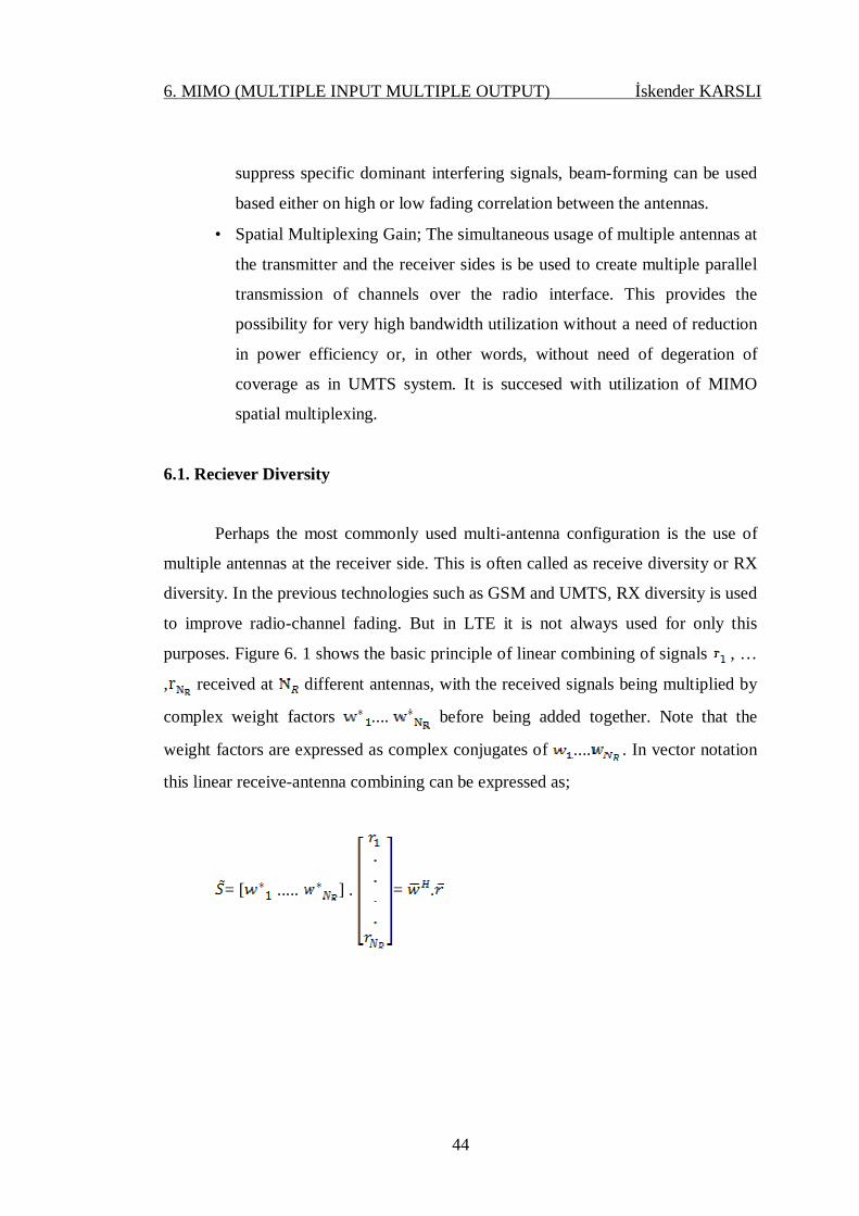
6. MIMO (MULTIPLE INPUT MULTIPLE OUTPUT) İskender KARSLI
44
suppress specific dominant interfering signals, beam-forming can be used
based either on high or low fading correlation between the antennas.
• Spatial Multiplexing Gain; The simultaneous usage of multiple antennas at
the transmitter and the receiver sides is be used to create multiple parallel
transmission of channels over the radio interface. This provides the
possibility for very high bandwidth utilization without a need of reduction
in power efficiency or, in other words, without need of degeration of
coverage as in UMTS system. It is succesed with utilization of MIMO
spatial multiplexing.
6.1. Reciever Diversity
Perhaps the most commonly used multi-antenna configuration is the use of
multiple antennas at the receiver side. This is often called as receive diversity or RX
diversity. In the previous technologies such as GSM and UMTS, RX diversity is used
to improve radio-channel fading. But in LTE it is not always used for only this
purposes. Figure 6. 1 shows the basic principle of linear combining of signals , …
, received at different antennas, with the received signals being multiplied by
complex weight factors .... before being added together. Note that the
weight factors are expressed as complex conjugates of .... . In vector notation
this linear receive-antenna combining can be expressed as;
= [ ..... ] . = .

6. MIMO (MULTIPLE INPUT MULTIPLE OUTPUT) İskender KARSLI
45
Figure 6.1. Linear receive-antenna combining (Dahlman, Parkvall, Sköld and
Beming, 2008 )
Figure 6.1 and the equation outlines the linear receive-antenna combining in
general. Different specific antenna-combining approaches are available then it differs
with choice of the weight vector . Lets assume that the transmitted signal is only
subject to non-frequency-selective fading. There is no radio channel time dispersion.
The signals received at the different antennas in Figure 6.1 can be expressed as;
where s is the transmitted signal, the vector consists of the complex
channel gains, and the vector consists of the noise corrupting the signals received
at the different antennas.

6. MIMO (MULTIPLE INPUT MULTIPLE OUTPUT) İskender KARSLI
46
6.2. Transmit Diversity
The transmit diversity provides additional source of diversity for averaging
out the channel variation either for operation at higher UE speeds or for delay
sensitive services at both low and high UE speeds. In the standardization phase
different types of transmit diversity schemes were discussed and evaluated for both
two transmit antennas and four transmit antennas cases. In the first part of this
chapter, we study the details of these various schemes. In the second part, we will
elaborate on the transmit diversity scheme used in the LTE system.
6.2.1. Cyclic Delay Diversity (CDD)
In the cyclic delay diversity (CDD) scheme when applied to an OFDM
system, delayed versions of the same OFDM symbol are transmitted from multiple
antennas as shown in Figure 6.2. Let be the sequence of modulation
symbols at the input of IFFT, then the sequence of samples at the output of the IFFT
can be written from the equation below;
Where k,n = 0, 1, . . . , (N − 1)
The sequence of samples at the output of the IFFT is
cyclically shifted before transmission from different antennas as shown in figure
figure 6.2. It can be consider that cyclic delay of 0, 1, 2 and 3 samples are transmitted
from antenna 0, 1, 2 and 3 respectively. It It should be noted that cyclic delay is
applied before adding the cyclic prefix (CP) and, therefore, there is no impact on
multi-path robustness of the transmitted signal. A cyclic delay diversity scheme can
be implemented in the frequency domain with a phase shift of applied to

6. MIMO (MULTIPLE INPUT MULTIPLE OUTPUT) İskender KARSLI
47
OFDM subcarrier k transmitted from the pth transmit antenna. The angle for the
pth transmit antenna is given as:
where is the cyclic delay in samples applied from the pth transmitting
antenna.
Figure 6.2. Cyclic Delay Diversity (CDD) scheme (Khan, 2009)
Simple presentation of cyclicly shifted subcarriers are shown in figure 6.3
below. Note that CP is also applied to each OFDM symbol before transmitting.
S1 S2 S3 S4
0 1 2 3 Ant03 0 1 2 Ant12 3 0 1 Ant21 2 3 0 Ant3
Figure 6.3. Cyclicly Shifted Subcarriers
6.2.2. Space Frequency Block Coding (SFBC)
In LTE, transmit diversity is implemented by using Space Frequency Block
Coding (SFBC). SFBC is a frequency domain adaptation of Space-time Block
Coding (STBC) also known as Alamouti coding where encoding is done in

6. MIMO (MULTIPLE INPUT MULTIPLE OUTPUT) İskender KARSLI
48
antenna/frequency domains rather than in antenna/time domains. In this approach
during any symbol period, two data symbols are transmitted simultaneously from the
two transmit antennas. In this scheme, the two symbols are sent on two different
frequencies, for example, on different subcarriers in an Orthogonal Frequency
Division Multiplexing (OFDM) system as shown in Figure 6.4. Let represent
the signal transmitted from the pth antenna on the kth subcarrier, then:
Figure 6.4. STBC and SFBC transmit diversity schemes for 2-Tx antennas. (Khan,
2009)
6.3. Spatial Mutiplexing
In the previous section, we examined how multiple antennas can be used to
provide the diverstiy gain. The transmission diversity improves the link performance
in the case of high mobilty. Transmit diversity is also useful for delay-sensitive
services. Since only a single data stream is always transmitted in transmit diversity, it
has no effect on data rates to reach peak values. Multiple transmission antennas
usage in eNB together with multiple receiver antennas at UE can be used to achieve
higher peak data rates by enabling multiple data stream transmission between eNB
and UE by using MIMO spatial multiplexing mode. The MIMO spatial multiplexing

6. MIMO (MULTIPLE INPUT MULTIPLE OUTPUT) İskender KARSLI
49
also improves cell capacity and throughput since UEs in good channel conditions can
use multiple streams transmissions. Spatial multiplexing is a special multiplexing
technique where different data streams are transmitted and recieved through several
independent (spatial) channels by using multiple antennas. As a result the higher the
number of antennas, the higher the number of data transmission rate. Main benefits
of spatial multiplexing;
• It is not needed additional power
• There is no additional bandwidth requirement
Of course, as in many areas of science, there is a theoretical limits in amount
of data that can be passed along a specific channel in the presence of noise. The
maximum amount of data that can be carried by a radio channel is limited by the
physical boundaries defined under Shannon's Law. Shannon's law defines the
maximum rate at which error free data can be transmitted over a given bandwidth in
the presence of noise. It is usually expressed in the form;
Where C is the channel capacity in bits per second, W is the bandwidth in
Hertz, and S/N is the SNR (Signal to Noise Ratio).
From this it can be seen that there is a limit on the capacity of a channel with
a given bandwidth. And the capacity is also limited by the signal to noise ratio of the
received signal. So a suitable way to increase the channel capacity is looking as
modulation scheme decision. The channel capacity can be increased by using higher
order modulation schemes, but these of course require a better signal to noise ratio.
Thus it can be said that, a balance exists between the data rate and the allowable error
rate, signal to noise ratio and power that can be transmitted.
As we mentioned to take advantage of the additional throughput capability,
MIMO utilizes multiple antennas in both transmitter and reciever part. In many
MIMO systems, just two antennas are used, but it is possible to use more antennas to

6. MIMO (MULTIPLE INPUT MULTIPLE OUTPUT) İskender KARSLI
50
increase throughput. Note that, in any case for MIMO spatial multiplexing the
number of receive antennas must be equal to or greater than the number of transmit
antenna . To take advantage of the additional throughput offered, MIMO wireless
systems utilize a matrix mathematical approach. Therefore A MIMO channel
consists of channel gains and phase information for links from each of the
transmission antennas to each of the receive antennas as shown in Figure 6.5. Then,
the channel for the M × N MIMO system consists of an N × M matrix given
as:
where represents the channel gain from transmission antenna j to the
receive antenna i. (Khan, 2009)
Figure 6.5. MxN Spatial Multiplexing
Consider 3x3 spatial multiplexing system. Then , , are transmitted the
data streams from antennas 1, 2, and 3. By this idea recieved signal streams , ,
are then;
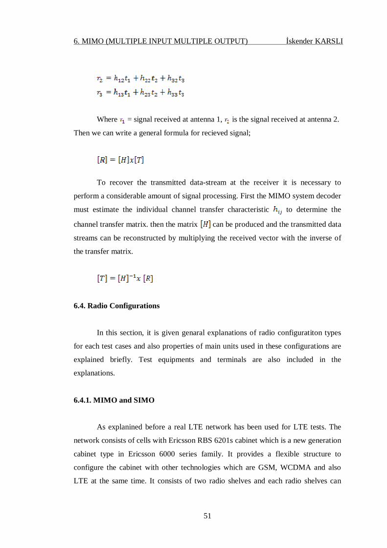
6. MIMO (MULTIPLE INPUT MULTIPLE OUTPUT) İskender KARSLI
51
Where = signal received at antenna 1, is the signal received at antenna 2.
Then we can write a general formula for recieved signal;
To recover the transmitted data-stream at the receiver it is necessary to
perform a considerable amount of signal processing. First the MIMO system decoder
must estimate the individual channel transfer characteristic to determine the
channel transfer matrix. then the matrix can be produced and the transmitted data
streams can be reconstructed by multiplying the received vector with the inverse of
the transfer matrix.
6.4. Radio Configurations
In this section, it is given genaral explanations of radio configuratiton types
for each test cases and also properties of main units used in these configurations are
explained briefly. Test equipments and terminals are also included in the
explanations.
6.4.1. MIMO and SIMO
As explanined before a real LTE network has been used for LTE tests. The
network consists of cells with Ericsson RBS 6201s cabinet which is a new generation
cabinet type in Ericsson 6000 series family. It provides a flexible structure to
configure the cabinet with other technologies which are GSM, WCDMA and also
LTE at the same time. It consists of two radio shelves and each radio shelves can

6. MIMO (MULTIPLE INPUT MULTIPLE OUTPUT) İskender KARSLI
52
house up to 6 Radio Units (RU). Each RU has a 20 Mhz bandwidth and up to 60 W
of output power which is adjusted in steps of 20 W. The main functions of RU’s are;
• Transceiver (TRX)
• Transmitter (TX) amplification
• Transmitter/Reciever (TX/RX) Duplexing
• TX/RX filtering
Number of possible Radio Configurations are listed in following Table 6.1. In
our thesis first two configurations have been applied.
Table 6.1. Possible Radio Cofigurations Configuration No of Radio Units Output Povver 3x20MHzMIMO 6 20+20 or 40+40 or 60+60 3x20 MHzSIMO 3 20 or 40 or 60 6x20 MHz 6 60 6x20 MHzMIMO 12 60 + 60
Simple hardware representation of MIMO and SIMO configuration has been
shown in figure 6.6. From the table1 in MIMO configuration there are 2 Radio Units
used in each cell and totally 6 RU’s in each site. Since it is used 2 Transceiver Radio
units in our cells we can say our system as 2*N MIMO system. On the other hand for
SIMO confıguration it requires 1 RU for each cells and totally 3 RUs in a site. But
please don’t forget, only one cell is activated and other cells are halted during the
tests.
Figure 6.6. Simple Hardware Representation of MIMO and SIMO configurations

6. MIMO (MULTIPLE INPUT MULTIPLE OUTPUT) İskender KARSLI
53
6.4.2. Dual Carrier
DC HSPA (Dual Cell HSPA) test has been carried out in a real Ericsson 3G
HSPA network that consists of cells with 6000 series cabinets. DC-HSDPA is a new
feature that comes with 3GPP Release 8. Major benefits of this feature is;
• Doubling DL Throughput with a peak throughput of 42Mb/s within the
cell
• Increase of HSDPA coverage
• Increase cell capacity
We know that the current bandwidth in UMTS/HSPA is 5 MHz. In Release 8
downlink, it is possible to increase data rates using either a combination of MIMO
and 64QAM or dual-cell HSDPA for operation on two 5MHz carriers with 64QAM,
data rates reach up to 42Mbps. In our thesis we used dual-cell HSDPA for the test
case. Dual cell approach provides higher throughput rates by combining two adjacent
5 MHz carriers as shown in figure 6.7 below. In this configuration, it is possible to
achieve a doubling of the 21 Mbps maximum rate available on each channel to 42
Mbps with a less expensive infrastructure upgrade. Since it doubles the user
throughout, we can say that this feature also increases cell capacity. Dual Cell
operation looks cheaper way than the usage of MIMO. Because MIMO needs
additional hardware usage which effects costs.
Figure 6.7. Dual Carrier Operation

6. MIMO (MULTIPLE INPUT MULTIPLE OUTPUT) İskender KARSLI
54
Dual-Cell assumes that both the 5MHz bands are adjacent. If they are not
adjacent then the better term to refer for DC is Dual-Carrier. A dual-carrier user can
be scheduled in the primary serving cell as well as in a secondary serving cell with
two parallel HS-DSCH transport channels as shown in figure 6.8. One of the carrier
can be configured as primary serving cell.
Figure 6.8. Parallel Operation of Dual Carrier HSPA
All physical layer procedures and non HSDPA related channels are included
in the primary serving cell. As a consequence, the dual-carrier feature also provides
an efficient load balancing between carriers in one sector. In Dual carrier
configuration, two transport blocks can be transmitted on their respective cells using
a different number of channelization codes as shown in the figure 6.7. We know
from the UMTS knowledges, if a UE is served by two cells of same node-b, we call
this event as softer handover. DC case can be accepted similar to this event but there
are minor differences in both Layer 2 and physical layer design. There are two
HARQ processes per TTI for dual carrier transmission/reception. So, at the physical
layer, dual carrier transmission can be tought as independent transmissions over 2
HS-DSCH channels, each having associated downlink and uplink signalling.
Figure 6.10 shows the architecture of MC-HSDPA. There are two
connections established for UE, one is serving cell and the other one is secondary
cell as shown in the figure. Notice that, in DL, two carriers are used while in UL
direction only one carrier is used for transmission.

6. MIMO (MULTIPLE INPUT MULTIPLE OUTPUT) İskender KARSLI
55
Figure 6.9. MC-HSDPA Architecture Overview
Physical layer structure can be seen from the figure 6.11 below. Primary
serving cell has all the physical channels, including DPCH/F-DPCH, EHICH , E-
AGCH, and E-RGCH. Secondary HS-DSCH cell functions as suplemantary cell
which have CPICH, HS-SCCH and HS-PDSCH physical channels. Please note that
in UL there is only used cell is primary serving cell.
Figure 6.10. Physical Channel Configuration

6. MIMO (MULTIPLE INPUT MULTIPLE OUTPUT) İskender KARSLI
56
Physical channels in Downlink;
• P-CPICH - Primary Common Pilot Channel
• DPCH (Dedicated Physical Channel) One per UE
• HS-SCCH High Speed Shared Control Channel
• HS-PDSCH High Speed Physical Downlink Shared Channel
• E-HICH
• E-AGCH
Physical channels in Uplink;
• DPCCH - Dedicated Physical Control Channel
• HS-DPCCH High Speed Dedicated Physical Control Channel
• E-DPCCH
• E-DPDCH
6.5. Test Terminals
2 types of terminals have been used in the tests. These terminals are;
• Samsung 4G USB modem (GT-B3710)
Samsung 4G USB modem is a MIMO compatible modem which is used in
Test Case 1 and Test Case 2. The modem supports 2.6GHz band for LTE service.
Samsung’s LTE solution is fully compliant with the latest 3rd Generation Partnership
Project (3GPP) LTE Release 8 (Rel-8) standard and its LTE UE category is CAT 3.
Table 6.2 shows the peak data rates according to LTE UE categories. From the table
since our modem is category 3 peak downlink data rate is 102.048Mb/s, uplink is
51.024Mb/s and it does not support 64 QAM in UL direction.

6. MIMO (MULTIPLE INPUT MULTIPLE OUTPUT) İskender KARSLI
57
Table 6.2. Peak Data Rates for LTE UE Categories
UE Category Peak Downlink Data Rate (Mbps)
Downlink Antenna Configuration (eNB
Transmit x UE Recieve)
Peak Uplink Data Rate
Support For 64 QAM in Uplink
Category 1 10,296 1x2 5,16 NoCategory 2 51,024 2x2 24,456 NoCategory 3 102,048 2x2 51,024 NoCategory 4 150,752 2x2 51,024 NoCategory 5 302,752 4x2 73,376 Yes
• E372 Huawei dual-carrier 42 Mb/s
E372 Huawei support 42 Mb/s HSPA dual carrier downlink and 11 Mb/s
uplink services. E372 has been used in test case 3. It support maximum 15 HS-
DSCH codes. It’s HSPA UE category is 24 and 3gpp release 8.
Table 6.3. List of HSPA UE Categories (Q: QPSK, 16: 16QAM, 64: 64QAM) based on downlink performance 4G Americas, 2011b)
6.6. Test Tools
TEMS investigations 11.0.2 has been used as a test tool for all tests. TEMS is
a well known tool which is a product of ASCOM and TEMS investigations 11.0.2
version is released on July 23, 2010. It supports GSM, HSPA and LTE technologies.

6. MIMO (MULTIPLE INPUT MULTIPLE OUTPUT) İskender KARSLI
58

7. TEST CASES İskender KARSLI
59
7. TEST CASES
One of the purpose of this thesis is to explain the actual reason of throughput
increase if it is related with technology change or MIMO usage. To explain this, It
has been investigated the effect of MIMO usage in a real LTE system. At the same
time It has been also carried out another test scenario in a real HSPA network to
make a comparison with LTE cases. Test scenarios have been carried out in 3 cases.
• Test Case 1: Multiple Input Single Output (MIMO)
• Test Case 2: Single Input Single Output (SIMO)
• Test Case 3: HSPA Dual Carrier
To carry out the test scenairos it has been selected an industrial region
environment and taken outdoor drive test measurements for a fixed predefined route.
The reason for selecting the industrial environment is to recieve better signal strength
for having better throuhput since the spaces between buildings are much more than
other environments. During test, it has been especially cared about to take all signal
strength ranges to observe the performace efficiently. In Results and Analysis
chapter, signal strengths and throughput results have been concluded and compared
in a table for each test cases. Physical layer values of the cases have been calculated
and compared with each other for analysis.
Figure 7.1. Test Route

7. TEST CASES İskender KARSLI
60
7.1. Test Case 1: Multiple Input Multiple Output (MIMO)
MIMO is a multiple antenna technique to enhance throughput or coverage of
a cell in a mobile system. There are two modes of MIMO which are spatial
multiplexing and transmit diversity as explained in previous chapters. Since the main
subject always emphasised in broadband market is high throughput while subscribers
are in mobile state so it is more proper to test MIMO in spatial multiplexing mode. In
this thesis LTE cell is configured as 2x2 spatial multiplexing mode of MIMO.
7.1.1. Materials and Configurations for Test Case 1
In this case, data is transmitted from two TX antennas and recieved by two
RX antennas as shown in the figure 7.1. TX part represents the base station side RX
side represents terminal side in the figure. It has been used an 18 dBi gain cross
polarized antenna which has a horizontal beamwidth of 58 degrees and 6.2 degrees
of vertical beamwidth in the cell. Other feeder and antenna properties are given in the
Table 7.1.
Figure 7.2. 2x2 MIMO Configuration

7. TEST CASES İskender KARSLI
61
Table 7.1. Antenna and Feeder Spesifications Antenna And Feeder SpesificationsAntenna Height 23 (m)Antenna Type Kathrein 800 10541 Antenna Frequency Range 2300–2690 MHzAntenna Gain 18 dBiImpedance 50 ohmsPolarization +45° and -45°Front-to-back ratio >25 dB Horizontal beamwidth 2490–2690 MHz 58 degrees (half power)Vertical beamwidth 2490–2690 MHz 6.2 degrees (half power) Antenna Tilt 3Azimuth 0Feeder Type 7/8" 50 ohmsFeeder Length 12 (m)
In MIMO case, it has been utilized 2 RUs for 2*2 MIMO configuration and
remember that an RU has a 20Mhz bandwidth and up to 60W of power. Since there
is only one subscriber within the cell and we desire to take maximum throughput, it
will be dedicated one subcarrier with 20Mhz bandwidth to only one subscriber to
take maximum throughput as shown in Figure 7.3.
Figure 7.3. One subcarrier with 20Mhz bandwdith
Table 7.2. RU Configuration Radio Unit Configurations for MIMORadio Configuration for MIMO 1×20 MHz *Number of Radio Units 2Output power (W) 40+40TX Frequency 2620-2640 (Mhz)RX Frequency 2500-2520 (Mhz) * One cell is active and other cells are halted during the tests.

7. TEST CASES İskender KARSLI
62
7.1.2. Test Results
Reference Signal Recieved Power (RSRP) and Physical Layer PDSCH
Throughput measured by the terminal is plotted in figure 7.4. It can be easily
concluded that there is a direct correlation between RSRP and throughput. For low
RSRP samples it has been measured low throughput. But it is very exciting that even
in the values below -100dB’s, the throughput is still maintain above 30Mb/s.
Figure 1.25. Serving Cell RSRP Plot for MIMO Case
Figure 7.4. RSRP vs PDSCH Phy Throughput Plot for MIMO Case
It can be seen from the figures below that PDSCH throughput values of
MIMO case is accumulated between 35Mb/s and 70Mb/s which is 93.8% of all
samples. And it is seen that the MIMO configured cell has served better than 70Mb/s
in 5.8 percent of all test.
Figure 7.5. Serving cell RSRP and PDSCH Phy distribution for MIMO case

7. TEST CASES İskender KARSLI
63
During the MIMO test, 3 types of modulation scheme has been used in DL
direction on the other hand 2 types of modulation scheme have been used in UL
direction. The left of the Figure 7.8 shows that majority of the modulation types are
64QAM and 16QAM. It has been recieved QPSK scheme only in small part of the
test which the lowest signal strength of the test. We had emphasised the correlation
between throughput and signal strength. Actually we know that throughut is
depended on used modulation scheme. At majority of the test it has been recieved
64QAM scheme and even in lower signal levels still we have 16QAM scheme as can
be seen from the signal plots below. It tends to a satisfied and sufficient avarege
throughput experience for user. In UL direction the main modulation scheme used is
16QAM except a small quantity of samples.
Figure 7.6. PSDCH and PUSCH Modulation Plot for MIMO Case We know that in MIMO 2 transport blocks (TB0 and TB1) are trasfered
simultaneously. Since they are transfered at same modulation in majority of the test.
It has been only included TB0 plot for analysis as shown in figure 7.8. We know
that;
• QPSK: 1 symbol 2 bits
• 16QAM: 1 symbol 4 bits
• 64QAM: 1 symbol 6 bits

7. TEST CASES İskender KARSLI
64
Distribution of the modulations for PDSCH and PUSCH is given in the table;
Table 7.3. Modulations Distribution for MIMO Test Case.
64QAM 55% 16QAM 83%16QAM 40% QPSK 17%QPSK 5%
DL UL
Figure 7.10 shows that during test duration it has been always used 2
transport blocks. 2 Transport Block usage percentage is 100.
Figure 7.7. Used Transport Blocks in MIMO 7.2. Test Case 2: Single Input Multiple Output (SIMO)
Between MIMO and SIMO hardware configuration, main difference is the
number of Radio Units. Additionally it has been made some parameter changes.
Antenna and feeder spesificatios are all same with SIMO case which is given in table
7.1.
7.2.1. Materials and Configurations for Test Case 2
In SIMO case spatial multiplexing is deactivated. To configure SIMO, some
parametric changes are applied and also one radio unit is deactivated. In SIMO case
only 1 TB is transferred to the terminal but terminal has two RX antenna as shown in
figure 7.11.

7. TEST CASES İskender KARSLI
65
Figure 7.8. SIMO Configuration
In SIMO case, 20Mhz bandwidth is still dedicated to single user to give
maximum throughput. The RU configuration is given in Table 7.4.
Table 7.4. RU Configuration Radio Unit Configurations for SIMORadio Configuration for MIMO 1×20 MHz *Number of Radio Units 1Output power (W) 40TX Frequency 2620-2640 (Mhz)RX Frequency 2500-2520 (Mhz)
7.2.2. Test Results
From the SIMO signal test plots below it seems a negative effect on coverage
compared to the MIMO. It is an expected situation since there is only one TB
transferred. Average RSRP in SIMO is -86 dbm while in MIMO -82.18dbm.
However in SIMO it is transferred one TB instead of two as in MIMO, maximum
throughput is not decreased to half of the maximum throughput in MIMO. Maximum
throughput in SIMO is 49.9Mb/s while in MIMO 76Mb/s.

7. TEST CASES İskender KARSLI
66
Figure 7.9. RSRP vs PDSCH Phy Throughput Plot for SIMO Case
PDSCH Throughput values are accumulated above 35Mb/s. Even in low
signal strengths throughput is not decreased below 17Mb/s.
Figure 7.10. Serving Cell RSRP and PDSCH Phy Distribution for SIMO Case
There are two modulation schemes used in DL which are 64QAM and QPSK
on the other hand in UL used modulation schemes are 16AQM and QPSK as shown
in the figure 7.15. In the region shown in left plot, it is seen that the radio conditions
are not so bad but used modulation scheme is QPSK. Because of that reason it has
been served with low throughput in this region. However it looks like a problem with
test measurements, it doesn’t effect our results since we calculate median values of
each KPI. And the other interesting point is there is not 16QAM modulation used in
PDSCH modulation, even in lowest signal levels it is still continious to serve with
6QAM modulation.
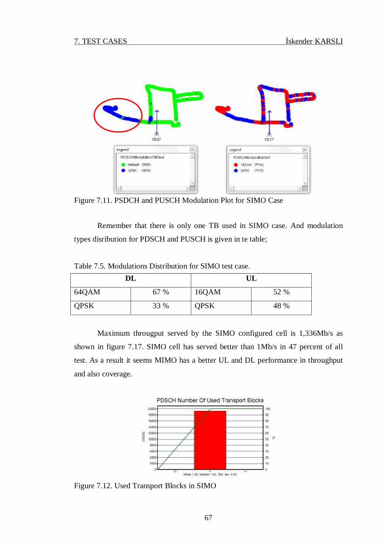
7. TEST CASES İskender KARSLI
67
Figure 7.11. PSDCH and PUSCH Modulation Plot for SIMO Case
Remember that there is only one TB used in SIMO case. And modulation
types disribution for PDSCH and PUSCH is given in te table;
Table 7.5. Modulations Distribution for SIMO test case. DL UL
64QAM 67 % 16QAM 52 %
QPSK 33 % QPSK 48 %
Maximum througput served by the SIMO configured cell is 1,336Mb/s as
shown in figure 7.17. SIMO cell has served better than 1Mb/s in 47 percent of all
test. As a result it seems MIMO has a better UL and DL performance in throughput
and also coverage.
Figure 7.12. Used Transport Blocks in SIMO

7. TEST CASES İskender KARSLI
68
7.3. Test Case 3: HSPA Dual Carrier
In previous sections it is given MIMO and SIMO tests which are carried in a
trial LTE network. As we mentioned before these tests are carried out within a single
cell, all other cells are deactivated during the tests. But in Dual Carrier HSPA case,
test is carried out within a real network. But from the signal plot below shows that
there are there cells served during the test and these cells are belong to same node b.
Figure 7.13. Serving Cells signal plot
Serving Cell Ratios are given as;
SCR 153 : 58.59 %
SCR 161 : 23.14 %
SCR 169 : 18.27 %
7.3.1. Materials and Configurations for Test Case 3
Since there is not only one cell in our test case it is allowed to make
handovers. It is given main serving cell properties in this chapter. In our test
scenario, it has been used Kathrein 742 215 antenna whose horizontal and vertical
pattern characteristics and gain are similar with LTE cases. Note that the antenna
height in DC case is 26m which is 3 meters higher than LTE cases. Other difference
is related with feeder type. Since It is used Ericsson 6601 cabinet as we mentioned
before, there is no feeder loss in DC case. Table 7.6 shows all physical properties of
the cell.
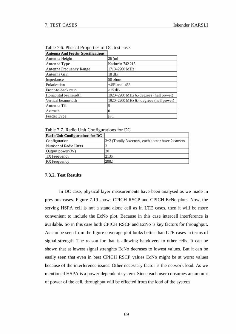
7. TEST CASES İskender KARSLI
69
Table 7.6. Phsical Properties of DC test case. Antenna And Feeder SpesificationsAntenna Height 26 (m)Antenna Type Kathrein 742 215 Antenna Frequency Range 1710–2200 MHzAntenna Gain 18 dBiImpedance 50 ohms Polarization +45° and -45°Front-to-back ratio >25 dB Horizontal beamwidth 1920–2200 MHz 65 degrees (half power)Vertical beamwidth 1920–2200 MHz 6.4 degrees (half power) Antenna Tilt 5Azimuth 0Feeder Type F/O
Table 7.7. Radio Unit Configurations for DC Radio Unit Configurations for DCConfiguration 3*2 (Totally 3 sectors, each sector have 2 carriersNumber of Radio Units 3Output power (W) 30TX Frequency 2136RX Frequency 2982
7.3.2. Test Results
In DC case, physical layer measurements have been analysed as we made in
previous cases. Figure 7.19 shows CPICH RSCP and CPICH EcNo plots. Now, the
serving HSPA cell is not a stand alone cell as in LTE cases, then it will be more
convenient to include the EcNo plot. Because in this case intercell interference is
available. So in this case both CPICH RSCP and EcNo is key factors for throughput.
As can be seen from the figure coverage plot looks better than LTE cases in terms of
signal strength. The reason for that is allowing handovers to other cells. It can be
shown that at lowest signal strenghts EcNo decrases to lowest values. But it can be
easily seen that even in best CPICH RSCP values EcNo might be at worst values
because of the interference issues. Other necessary factor is the network load. As we
mentioned HSPA is a power dependent system. Since each user consumes an amount
of power of the cell, throughput will be effected from the load of the system.

7. TEST CASES İskender KARSLI
70
Figure 7.14. CPICH RSCP and CPICH EcNo Plot
Ideal value of EcNo is accepted around -12 dBm. EcNo figure below looks
the test route is a little bit polluted because 73 percent of the EcNo samples are less
then -12 dBm. It has a negative effect on throughput even if the coverage is
satistified. Median value of RSCP is already calculated as -64.54 dBm.
Figure 7.15. CPICH RSCP and CPICH EcNo Distribution Lets look at the region 1 in the figure 7.21 below, in this region we have good
RSCP samples but bad EcNo values. This causes low physical DL and UL
througputs. If we look at the region 2, we see bad RSCP and bad EcNo values but
throughput values look better than the region 1. It is tought that the system load in
region 2 is more relaxed than region 1.

7. TEST CASES İskender KARSLI
71
Figure 7.16. Physical Layer Served Thr and HS UL EDCH Throughput Plot
HS Physical served median throughput in DL is calculated 10.676 Mb/s and
median throughput in UL is 258 Kb/s. DC HSPA cell has served better than 10Mb/s
in 55 percent of all test. It is seen that in HSPA DC case throughput vales
accumulated between 5Mb/s and 15 Mb/s. And the maximum value taken in this case
is 26.949 Mb/s.
1
2

7. TEST CASES İskender KARSLI
72

8. RESULTS AND ANALYSIS İskender KARSLI
73
8. RESULTS AND ANALYSIS
In this thesis, 3 test cases have been carried out for analysing the performance
effects of the multiple antenna usage in an LTE system together with technology
comparisons with LTE and Dual carriers HSPA networks. All test cases are studied
and analysied in the previous sections in detail. The following table 8.1 gives a result
table that consists of throughput and coverage values of each test cases. And the
latter table gives theorical speeds of each cases.
Table 8.1. Throughput and Coverage Comparisons Between Test Cases LTE MIMO LTE SIMO Dual Carrier
PDSCHPhyThroughputkbits-Max 76096 49848 HSPhyServedThroughputkbits-Max 26949
PDSCHPhyThroughputkbits-Median 56440 23752 HSPhyServedThroughputkbits-Median 10510PUSCHPhyThroughputkbits-Max 1912 1336 HSULEDCHThroughputkbits-Max 1047
PUSCHPhyThroughputkbits-Median 1224 520 HSULEDCHThroughputkbits-Median 255ServingCellRSRPdBm-Median -77 -83 RSCP-Median -64.54
Table 8.2. Theoretical Speed Vales in DL Theorical Speed DL
LTE MIMO 2*2 172.8Mb/s
LTE SIMO 1*2 91.2Mbs
HSPA Dual Carrier 42mb/s
8.1. In Terms of Throughput
From the table 8.1 it can be seen that the best througput values are taken with
the LTE cases. 76Mb/s which is taken with LTE MIMO is very satisfied value for a
UE while it is in mobile. Additionally, As it is emphasised in the Test Case section
PDSCH throughput values of LTE MIMO case is accumulated between 35Mb/s and
70Mb/s which is 93.8% of all samples. For SIMO case the distrubution is smilar to
MIMO case. On the other hand, in HSPA DC, however the maximum througput is
26Mb/s the acummulation of the values is between 5Mb/s and 15 Mb/s. This results
show that the LTE cells serve without decreasing the excessive values of

8. RESULTS AND ANALYSIS İskender KARSLI
74
throughputs. From the user experience aspect this means that UE recieves very
satisfiable throughputs during the connection as compared to the HSPA network. Of
course it is needed to remember again the HSPA network is a real, alive network.
One of the objective of this thesis is to investigate the reason of the throughput
increase if it is related with technology difference or not. To show that it will be
more appropiate to take median values since it directly reflects the user experience. If
we look at the throghput increases between cases, downlink throughput increase
(according to the median value) between Dual Carrier and LTE SIMO is around 2.25
on the other hand throuhput difference between SIMO and MIMO is around 2.37
times. This results show that technology difference is a key factor of this throughput
increase but it is seen that MIMO usage improves the performance more
dramatically.
When we look at the maximum values, in MIMO case it was doubled the
count of antenna, as a result of this it was expected that it would be doubling the
throughput value of the SIMO case. But the test results showed that the maximum
throuhgput increase is around 1.5 times of SIMO value.
So it can be said that even if the MIMO usage not to double the maximum
throughput it is seen that it serves satisfied user experience when you look at the
overall median performance. Then it can be concluded that multiple antenna usage is
a usefull and efficent technigue to enhance the throughput performance of the
system. It only requies an additional radio unit and no need an extra antenna by
utilizing the other branch of the antenna. MIMO usage seems more beneficial for
dense areas than rural since it needs additional radio units. SIMO is more suitable for
rural sites because of the cost savings.
In our thesis it has not been carried out any test in uplink direction. Actually
theoretical speed in MIMO is 50Mb/s. Uplink values in our test is only related with
signalling.

8. RESULTS AND ANALYSIS İskender KARSLI
75
8.2. In Terms of Coverage
In MIMO, as we mentioned it is tranfered two transport blocks in each TTI, it
will enhance not only throughput but also coverage. As expected the best coverage
values are taken in Dual Carrier case since the test is carried out in a real system. It is
let to make handover. Then it is more convenient to compare only LTE cases for
coverage aspect. From the table it is seen that in MIMO case Median RSCP value for
serving cell is better than SIMO case. With these values, The loss on coverage is
reasonable compare to the loss on throughput. Then for cost-focused operators, it is
recommended that SIMO case looks more feasible configuration for rural areas as
compared to city centers. But, it should be known that these data speeds will not be
sufficent for users since the satisfaction levels grow continiously. For medium term it
might be expected that a new deployement process will be required to carry out from
SIMO to MIMO.
Then it is concluded that for phase 0, MIMO is more suitable configuration
for high data demands city centers and SIMO can be prefered especially for rural
areas. For medium term as demands get higher MIMO usage can be increased.
8.3 Key Diffrences Between Technologies
Table 8.3 answers why such a big throughput increases occur between
technology transitions.
Spectrum flexibility is one of the key difference between LTE and previous
technologies. LTE can operate in various frequency bands and can be deployed with
different bandwidths so that a different spectrum may allow efficient migration from
previous radio technologies to LTE. LTE has the widest channel bandwidth which is
expandable from 1.4 MHz to 20 MHz as shown in the table.
GSM uses a mixture of FDMA and TDMA as radio access technology which
are known as non-overlapping systems. On the other hand in UMTS, a fully overlap
system WCDMA is used as radio access technique. So, GSM is not a spectrum
efficient as much as UMTS since TDMA/FDMA utilizes non-overlapping channels.

8. RESULTS AND ANALYSIS İskender KARSLI
76
However UMTS needs less spectrum the GSM, interference is a big issue WCDMA
is a fully overlapping system. OFDM arises as a new tecnique coming with LTE
technology. OFDM is a an overlapping form of FDM technique. However it looks
not a spectrum efficient as much as WCDMA, it is more robust against interference.
From the table, it is seen that higher order modulation and MIMO support is
available as technology developes. These are additive factors of throughput increases
between technologies.
Besides all other factors mentioned here, probably the most important
evolution between technologies is related with TTI which defines the duration
between two subsequent user data. It directly effects the data throughput. LTE
proposes 1ms TTI duration, this value was 20 ms in GSM edge technology.
Advanced power control algorithms together with shorter TTI values reduces overall
interference of the system and as a result of this, subscribers can be scheduled with
higher order modulation schemes in each TTI.
Table 8.3. Key Properties of Each Technology
GSM EDGE GSM E-EDGE UMTS-R99 UMTS HSPA UMTS HSPA Dual Carrier LTE# RF Channel 124 124 12 12 12 flexible
Channel Bandwidth 200Khz 200Khz 5Mhz 5Mhz 10Mhz 1.4 to 20Mhz
Access Tcehnology FDMA-TDMA FDAMA-TDMA WCDMA WCDMA WCDMA OFDM
Overlap non-overlap non-overlap full-overlap full-overlap full-overlap partially-overlap
Modulation GMSK-8PSK 16QAM-32QAM QPSK QPSK-16QAM-64QAM QPSK-16QAM-64QAM QPSK-16QAM-64QAM
TTI 20ms 10ms 10ms 2ms 2ms 1ms
MIMO Support No No No Yes Yes Yes
Power Control Yes(new feature) Yes(new feature) Yes Yes Yes Yes

77
REFERENCES
4G AMERICAS 2011A. 3GPP Rel 10 and Beyond, Technical White Paper , Page 9,
51. http:// www.4gamericas.org.
4G AMERICAS, 2011B. Coexistence of GSM, HSPA and LTE Technical White
Paper, Page 5, 48. http:// www.4gamericas.org.
DAHLMAN, E., PARKVAL, S., SKÖLD, J. and BEMING, P., 2008. 3G Evolution
HSPA and LTE for Mobile Broadband. Academic Press of Elsevier, UK,
Page 43, 44, 48, 49, 50, 300, 301, 302.
JHA, U.S. and PRASAD, R., 2007. OFDM Towards Fixed and Mobile Broadband
Wireless Access. Artech House, USA, Page 54, 55.
KHAN, F., 2009. LTE For 4G Mobile Broadband. Cambridge University Press, UK,
Page 111, 124, 147, 148.
LANGTON S., 2004. “Orthogonal Frequency Divison Multiplex (OFDM) Tutorial”,
http://www.complextoreal.com/chapters/ofdm2.pdf (Access Date:
December 14th, 2012)
LESCUYER, P. and LUCIDARME, T., 2008. Evolved Packet System (EPS). John
Wiley & Sons, UK, Page 175.
THE NIELSEN COMPANY, 2011A. “Android Leads in U.S. Smartphone Market
Share and Data Usage”,
http://blog.nielsen.com/nielsenwire/consumer/android-leads-u-s-in-
smartphone-market-share-and-data-usage/ (Access Date: December 14th,
2012)
THE NIELSEN COMPANY, 2011B. “Average U.S. Smartphone Data Usage Up
89% as Cost per MB Goes Down 46%”,
http://blog.nielsen.com/nielsenwire/online_mobile/average-u-s-
smartphone-data-usage-up-89-as-cost-per-mb-goes-down-46/ (Access
Date: December 14th, 2012)
PEARSON C., 2011. Wireless Market Update: Innovations and Spectrum
Considerations

78
RYSAVY RESEARCH, 2012. Mobile Broadband Explosion, White Paper, Page 14.
http:// www.rysavy.com.
RYSAVY RESEARCH, 2010. Mobile Broadband Capacity Constraints And the
Need for Optimization. White Paper, Page 16. http:// www.rysavy.com.

79
BIOGRAPHY
İskender KARSLI was born on 1977, city of Adana, Turkey. He graduated
from the University of Gaziantep in Electrical and Electronical Engineering at 2002.
After graduation, he was completed his military service in 2003. In 2004, He started
working as a Tranmission Engineer in ADATEL AŞ which is a contrcator of
TURKCELL. After an 8 months job duration in ADATEL AŞ, He started Turkcell as
Access Network Transmission Engineer in 2005. He worked on same position until
the end of 2006. Between years 2006-2011 he worked as a GSM-UMTS Cell
Planning Engineer for TURKCELL. Since 2011 he has working as a Senior 2G-3G
Optimization Engineer at TURKCELL.