UNIVERSITY OF CONCEPCION - CHILE FACULTY OF …

UNIVERSITY OF CONCEPCION - CHILEFACULTY OF ENGINEERING

DEPARTMENT OF INDUSTRIAL ENGINEERING

Overall Optimization of Tidal Current Farm: a Case Study in

Chacao Channel, Chile

By:

Pablo Enrique Fierro Valdebenito

Thesis Supervisor:

Maichel M. Aguayo PhD.

Co-advisor:

Rodrigo de la Fuente G. PhD.

Concepcion, April 2020

Thesis Submitted to

POSTGRADUATE EDUCATIONUNIVERSITY OF CONCEPCION

For the Degree of

MASTER IN INDUSTRIAL ENGINEERING

ABSTRACT

Overall Optimization of Tidal Current Farm: a Case Study in Chacao Channel,

Chile

Pablo Enrique Fierro ValdebenitoMarch 2020

Thesis Supervisor: Maichel M. Aguayo PhD.Program: Master in Industrial Engineering

In this work, a mathematical model for the overall optimization of a Tidal Current Farm (TCF) is

presented. This model consists of Mixed Integer Programming (MIP) that solves a layout opti-

mization problem and cable routing problem, using a single model for this purpose. Besides, the

model estimates the economic profitability of the project through the calculation of Net present

value (NPV). The NPV must be maximized, which involves minimizing investment costs and

maximizing net cash flows, which are calculated by the number of devices to be occupied and

the amount of net energy produced by the TCF, respectively. Both the amount of energy pro-

duced and the investment costs are components of the objective function to be optimized. To

determine the efficiency of the proposed model, a case study of a TCF project located in the

Chacao Canal, Chile, is solved. Selected scenarios are tested, consisting of TCF of different

sizes. The results showed that the optimization model determines the best locations for turbines,

routing cables to connect them, and sets the economic profitability of the project. Compared

to previous work that used mathematical modeling to solve layout problems of this type, this

method obtains results in better computational times and is efficient with different cases.

Keywords: Tidal current farm, Optimization, Cable routing problem, Layout optimization,

mixed integer programming.

Master in Industrial Engineering, Postgraduate Education - University of Concepcion i

Contents

Abstract i

List of Figures iv

List of Tables v

1 Chapter 1. Introduction and Objectives 1

1.1 Introduction . . . . . . . . . . . . . . . . . . . . . . . . . . . . . . . . . . . . 1

1.2 Objectives . . . . . . . . . . . . . . . . . . . . . . . . . . . . . . . . . . . . . 1

2 Chapter 2. Problem Description 3

3 Chapter 3. Literature Review 6

3.1 Cable Routing Problem . . . . . . . . . . . . . . . . . . . . . . . . . . . . . . 6

3.2 Layout Optimization . . . . . . . . . . . . . . . . . . . . . . . . . . . . . . . 8

3.3 Research Gap . . . . . . . . . . . . . . . . . . . . . . . . . . . . . . . . . . . 10

4 Chapter 4. Methodology 11

4.1 Wake modeling in Tidal power farm . . . . . . . . . . . . . . . . . . . . . . . 11

4.2 Tidal Farm economic evaluation model . . . . . . . . . . . . . . . . . . . . . . 12

5 Chapter 5. Case Study 19

5.1 Bathymetry and current speed . . . . . . . . . . . . . . . . . . . . . . . . . . 19

5.2 Test cases . . . . . . . . . . . . . . . . . . . . . . . . . . . . . . . . . . . . . 20

6 Chapter 6. Computational Results 23

7 Chapter 7. Discussion 26

7.1 Parameter sensitivity . . . . . . . . . . . . . . . . . . . . . . . . . . . . . . . 26

7.1.1 Sensitivity to the energy price . . . . . . . . . . . . . . . . . . . . . . 26

Master in Industrial Engineering, Postgraduate Education - University of Concepcion ii

7.1.2 Sensitivity to opportunity cost . . . . . . . . . . . . . . . . . . . . . . 27

7.1.3 Sensitivity to current speed . . . . . . . . . . . . . . . . . . . . . . . . 28

7.1.4 Sensitivity to Limited Budget . . . . . . . . . . . . . . . . . . . . . . 28

7.2 Comparison with literature . . . . . . . . . . . . . . . . . . . . . . . . . . . . 31

7.3 Insights . . . . . . . . . . . . . . . . . . . . . . . . . . . . . . . . . . . . . . 32

8 Chapter 8. Conclusions 34

References 35

Master in Industrial Engineering, Postgraduate Education - University of Concepcion iii

List of Figures

4.1 The Jensen wake model . . . . . . . . . . . . . . . . . . . . . . . . . . . . . . 12

5.1 Chacao Channel: Location in Chile, Bathymetry and Speed current . . . . . . . 20

5.2 Zones in the Chacao Channel and set of cases . . . . . . . . . . . . . . . . . . 21

6.1 Results of TCF layout and cable routing . . . . . . . . . . . . . . . . . . . . . 24

7.1 Sensitivity analysis of energy price variation . . . . . . . . . . . . . . . . . . 26

7.2 Sensitivity analysis of opportunity cost . . . . . . . . . . . . . . . . . . . . . . 27

7.3 Sensitivity analysis of current speed variation . . . . . . . . . . . . . . . . . . 28

7.4 Sensitivity analysis of limited budget . . . . . . . . . . . . . . . . . . . . . . . 29

7.5 Cases to increase the budget . . . . . . . . . . . . . . . . . . . . . . . . . . . 30

Master in Industrial Engineering, Postgraduate Education - University of Concepcion iv

List of Tables

3.1 Location and cable routing problem reported in the literature . . . . . . . . . . 7

4.1 Notation for optimization model. . . . . . . . . . . . . . . . . . . . . . . . . . 15

5.1 Main technical and economic input data. . . . . . . . . . . . . . . . . . . . . . 22

6.1 Main economic results of the proposed model . . . . . . . . . . . . . . . . . . 23

Master in Industrial Engineering, Postgraduate Education - University of Concepcion v

Chapter 1. Introduction and Objectives

1.1. Introduction

Due to the limited capacity of the current energy resource, based mainly on fossils fuels, un-

conventional renewable energies are the main alternatives for the change of energy source, for

their condition of inexhaustible resource. Among the unconventional energy sources, the one

that comes from the tides, also known as Tidal Current Energy, has been highlighted in the last

time.

Tidal power plant is a facility that converts the kinetic energy of the sea current into electricity,

through devices called tidal turbines. By moving the turbine propellers, the energy produced is

transferred to alternators to convert it into electric energy. These plants are located in strategic

locations, with ideal natural characteristics for their operation (energy potential, current speed,

depth, among others). These plants represent a considerable economic cost, mainly due to the

installation and connection of each of the turbines, which has a high impact on the initial capital

investment.

This research presents a mathematical model that optimizes the layout of tidal current farm. The

proposed methodology solves the location of turbines on the farm, as well as the connection

path between the devices. The model determines, through economic indicators, whether or not

the project has economic profitability according to a given life span. Also, this study develops a

particular case of a tidal current farm and its installation in southern Chile.

1.2. Objectives

General objectives

To obtain a mathematical model that performs an overall assessment of a tidal turbine farm,

Master in Industrial Engineering, Postgraduate Education - University of Concepcion 1

applying that model on the Chacao Channel.

Specific objectives

1. To review existing literature to find references and formulations applied to Tidal Turbine

Farm Optimization.

2. To develop a mathematical programming model that determines the optimal cable layout

and routing, in addition to the economic profitability of the tidal turbine farm.

3. To collect data and information from the Chacao Channel.

4. To apply the model to different scenarios and cases.

The remaining of this work is organized as follows. Chapter 2 shows an overview of the problem

to be addressed in this study. In Chapter 3. a literature review is presented. Next, in Chapter 4, a

description of the model used to solve the location and cable routing problem for TCF is shown.

Case study with the parameters and data of the Chacao channel are presented in Chapter 5. The

computational results are shown in Chapter 6. Chapter 7 presents the discussions of the results

shown in the previous section. Finally, in Chapter 8, the main conclusions and future works are

shown.


Chapter 2. Problem Description

Over the last years, the renewable energy industry has been growing in importance due to tech-

nology development to take advantage of these energies, the falling technology costs, and rising

environmental concerns. Since the governments of the countries are interested in investing re-

sources to change fossil fuels, the production of green energy has attention both industrial and

academic. Among the renewable energy sources, Tidal current energy (TCE) is a renewable,

clean and sustainable alternative as it does not produce greenhouse gas. TCE is considered to

be one of the main resources for future electricity generation due to its energy potential; it is

experiencing a high technological development, being the ocean energy with the highest rate of

preparation and technological takeoff, according to the International Renewable Energy Agency.

(IRENA (2014)).Currently, there are 8 tidal power stations in the world, 4 in Europe (France,

Russia, United Kingdom, and the Netherlands), 3 in Asia (China and 2 plants located in South

Korea) and 1 in Canada, with a joint production of 530 MW. Moreover, 10 tidal power plants

will be built (5 in the UK, three in Russia and 2 in South Korea) to generate total energy of 2,000

MW (Neill et al. (2018).

In Chile, it has been shown that the southern part of the country is one of the most appropri-

ate sites in the world for electricity generation from marine resources, highlighting the research

done by Hassan (2009). In this scenario, different research has been done to analyze the techni-

cal feasibility of energy production in the Chacao Channel, located in Los Lagos Region. Guerra

et al. (2017) presented a field characterization study of the Chacao Channel. The results showed

that the channel has an average energy density of 5 kWm−2 at a depth not exceeding 60 m, which

means several areas are suitable for tidal current energy extraction. On the other hand, Villalon

et al. (2019) determined that, by installing an 8.4 MW tidal power station, it could generate a

total of 38.7 GWh per year, without exceeding the limits established by the Chilean electricity

standard or exceeding 7% of the allowed voltage level.


In a tidal power plant, the most important device is the tidal power turbine. These machines har-

ness the kinetic energy contained in the tide, to convert it into electricity with a transformer. The

tidal turbine can be installed in a layout called tidal current farm (TCF), for large-scale power

production. Evaluating a turbine farm project requires the consideration of two key economic

factors: investment costs and revenues from selling the generated energy.

To reduce investment costs and increase revenue, turbines must be located in the array in such

a way as to maximize the energy generated and that the cost of installation, civil and electri-

cal infrastructure becomes nor too high. This would be achieved by installing a large group of

turbines very close to each other. However, a large number of tidal turbines within an array

can reduce the overall efficiency of the tidal farm. So, it is necessary to consider the aerody-

namic interaction among multiple turbines to avoid large losses due to interference. As in wind

farm, the wake induced by a turbine is a zone of reduced velocity behind the device. Because

of this phenomenon called wake effect, downstream turbines extract less energy form the flow

than upstream ones, which has a negative impact on energy production. Therefore the analysis

of the wake effect is an important factor to assess the feasibility of the project. Another key

aspect of the development of marine energy projects is to determine the costs of subsea cables.

As in offshore wind farm (OWF), the amount of cable, its installation and subsequent periodic

maintenance represent a significant portion of the capital expenditure (CAPEX) made by project

investors. Both Lumbreras and Ramos (2011) and Quinonez-Varela et al. (2007) have demon-

strated that connection costs can be nearly 25% of the total investment cost. Making an optimal

design of electrical wiring can mean a considerable reduction in costs for the project budget.

This work presents a methodology, based on operations research (OR), to address the overall

optimization of a tidal power farm project. This methodology consists of a mixed integer pro-

gramming (MIP) approach which optimizes the individual location of turbines within the array

and solves the subsea cable routing problem for these devices. The proposed model not only

considers the loss of power resulting from the effect of the wake but also takes into account


power losses from transmission lines. Also, the model considers the costs of acquiring and in-

stalling the necessary equipment. The methodology introduced in this paper evaluates the results

throughout the whole life of the tidal farm according to the economic viability of the project,

determined by the Net Present Value (NPV). This provides useful economic and financial infor-

mation for investors willing to promote tidal power plants, allowing analysis of the economic

viability of future such projects. This study presents a case of a tidal current farm and its in-

stallation in the Chacao Channel. Finally, it contributes to evaluating a project that helps energy

independence mainly of the people of Isla de Chiloe, which is separated from the continent.


Chapter 3. Literature Review

This literature review considers both tidal current farm problems and offshore wind farm prob-

lems since the solution procedures are similar. This work focuses primarily on cable routing

problems and layout optimization to address the present problem. Table 3.1 shows, as a sum-

mary, the works of the literature related to the themes mentioned above. Three key criteria were

selected for the classification of literature. The first criterion considers whether or not the pa-

pers solved cable routing or layout optimization problems. For this criterion, only those studies

where the authors proposed a MIP were included. The second criterion is whether or not heuris-

tics (or metaheuristics) or exact algorithm solutions are used to solve the MIP showed. The third

criterion identifies whether the authors worked on an offshore wind farm (OWF) problem or a

tidal current farm (TCF). Finally, this review shows the objective function optimized.

3.1. Cable Routing Problem

Next, cable routing problems are presented and classified in Table 3.1. This problem arises

when a set of devices are installed and connected through cables. The routing of cables must be

determined to obtain the least design cost. The first optimization model to solve an OWF cable

routing problem was proposed by Fagerfjall (2010) in his master thesis. The model assumed

that all the turbines were connected to a single substation. Based on this model, various exten-

sions have been proposed adding aspects of Operations Research and some classic mathematical

models, including approaches to the Traveling Salesman Problem (TSP). Gonzalez-Longatt et al.

(2012) used a multiple TSP (mTSP) approach to solve the OWF power grid design optimization

problem. On the other hand, Srikakulapu and U (2017) presented a mTSP approach to get an

optimized routing of OWF, using Ant colony algorithm (ACO). Klein and Haugland (2017) de-

veloped an optimization model based on a TSP with distance and obstacle constraints between

turbines. This model optimizes a cable routing of an OWF considering the physical character-

istics of the seafloor. OWF-related papers are included, because the wind farm problems are

similar to tidal turbine farm problems, and solution methods are related as well. Finally, Vartdal


et al. (2018) used an mTSP approach to solve the cable routing problem for one or more hub

collectors in a simulated tidal farm.

Tabla 3.1: Location and cable routing problem reported in the literature

ReferenceProblem Solving Method Topic

Objective Function LimitationCable Routing Layout Heuristic Exact Method OWF TCF

Fagerfjall (2010) • • ◦ • • ◦ Max. power, Min. costs Two-phase solution, limited problem size

Serrano Gonzalez et al.(2010) ◦ • • ◦ • ◦ Net Present Value Limited number of turbines

Ituarte-Villarreal and Espiritu (2011) ◦ • • ◦ • ◦ Minimize cost No case study or losses by transmission

Gonzalez-Longatt et al.(2012) • ◦ • ◦ • ◦ Maximize electric power No real case study

Lumbreras and Ramos (2013) ◦ • • • • ◦ Minimize cost No wake effect, infeasibility for large-size problems

Funke et al. (2013) ◦ • • ◦ ◦ • Minimize cost No bathymetric effect or limited wafe modelling

Turner et al. (2014) ◦ • ◦ • • ◦ Minimize wind speed deficit Limited problem size

Bauer and Lysgaard (2015) • ◦ • • • ◦ Minimize cost No power losses or transmission losses

Kuo et al. (2015) ◦ • ◦ • • ◦ Maximize power Infeasibility for large-size problems

Pillai et al.(2015) • ◦ • ◦ • ◦ Minimize cost Two-phases heuristic, limited problem size

Funke et al. (2016) ◦ • • ◦ ◦ • Maximize profit Two-phases heuristic

Culley et al.(2016) • • • ◦ ◦ • Maximize profit Two-phases heuristic

Rodrigues et al.(2016a) ◦ • • ◦ • ◦ Minimize cost No real case study

Wetzik et al.(2016) • ◦ • ◦ • ◦ Minimize cost No real case study

Rodrigues et al.(2016b) ◦ • • ◦ • ◦ Maximize power No case study or power losses

Shim y Kim (2016) • ◦ • ◦ • ◦ Minimize cost Two-phases heuristic

Pillai et al. (2016) • ◦ • ◦ • ◦ Minimize cost Limited number of turbines

Kramer et ak. (2016) ◦ • • ◦ ◦ • Maximize profit Two-phases heuristic

Fischetti and Pisinger (2017) • ◦ • • • ◦ Minimize cost Limited problem size

Srikakulapu and U (2017) • ◦ • ◦ • ◦ Minimize cost No power losses or transmission losses

Klein and Haugland (2017) • ◦ ◦ • • ◦ Minimize cost No real case study

Amaral and Castro (2017) ◦ • • ◦ • ◦ Maximize power Limited problem size and restricted CPU time

Pillai et al.(2017) • ◦ • ◦ • ◦ Minimize cost No power losses or transmission losses

Gong et al.(2017) • ◦ • ◦ • ◦ Maximize power No case study or power losses

Dai et al. (2017) ◦ • • ◦ ◦ • Minimize cost No real case study

Fischetti and Pisinger (2018a) • ◦ • • • ◦ Minimize cost No power losses or transmission losses

Fischetti and Pisinger (2018b) • ◦ • • • ◦ Minimize cost Restricted CPU time

Vartdal et al. (2018) • ◦ ◦ • ◦ • Minimize cost Infeasibility for large-size problems

Zuo et al. (2018) ◦ • • ◦ • ◦ Maximize power No case study or losses by transmission

Wade et al. (2018) • ◦ • ◦ • ◦ Minimize cost Restricted CPU time

Fierro et al. (2020) • • ◦ • ◦ • Net Present Value Approaching wake effect equations

◦: not included, •: included

Various models based on Vehicle Routing Problem (VRP) approach have been proposed to solve

the cable routing problem. Bauer and Lysgaard (2015) used a mathematical model of Open Ve-

hicle Routing Problem (OVRP) to solve the cable routing at three OWF plants located off the

coast of England. An extension of this approach was presented by Fischetti and Pisinger (2017)

to avoid power losses, using a classic heuristic-based VRP approach. Also, Pillai et al. (2017)


used a classic VRP approach but based on a genetic algorithm to minimize routing costs. Gong

et al. (2017) proposed a sweep algorithm-based VRP approach to obtain specific cable paths,

depending on the different shapes and characteristics of electric cables. Later, Fischetti and

Pisinger (2018a) solved a similar cable routing problem with a hybrid VRP model. Fischetti and

Pisinger (2018b), in other work, addressed the same problem but taking account of the cable

losses.

Some optimization models have added distance restrictions to the cable routing problem. Pillai

et al. (2015) proposed a mixed integer linear programming model (MILP) with a Capacitated

Minimum Spanning Tree (CMST) approach to determine the optimal cable routing of an OWF

constrained by distances. In other work, Wedzik et al. (2016) used a MIP with a Minimum Span-

ning Tree approach to solve the cable routing of an OWF, considering the topology restrictions

and size of the electrical cables. Recently, the use of more complex algorithms has increased

to obtain optimal solutions, incorporating restriction characteristics of those algorithms to the

optimizations models. Shin and Kim (2016) proposed applications of the Minimum Cover Tree

(MCT) algorithm to improve a MIP with distance and substation location. On the other hand,

Pillai et al. (2016) used heuristics of Genetic Algorithm (GA) to minimize routing costs, Finally,

the use of particle algorithm was introduced by Wade et al. (2019) to reduce the overall electrical

costs of an OWF grid.

3.2. Layout Optimization

The layout optimization problem is one of the most studied tasks for both OWF and TCF. The

objective of this problem is to determine the best position array to locate the turbines. The wind

farm layout problem was introduced by Fagerfjall (2010) along with the cable routing model

mentioned above. Lumbreras and Ramos (2013) presented a MIP that minimizes the cost of

investment and considers the loss of power. Turner et al. (2014) developed a mathematical pro-

gramming model for the wind farm layout problem, taking account of the wake effect modeling.

Also, Kuo et al. (2015) extended that model with wake interactions based on energy balance.


On the other hand, a multi-objective economic and operational cost criteria to obtain the opti-

mal layout for an OWF is presented by Rodrigues et al. (2016b), as well as the consideration

of installation times of the electrical structures of the plants in another Work (Rodrigues et al.

(2016a)). Finally, Zuo et al. (2018) solved a layout problem with the collector system in offshore

wind farm and onshore substation.

Recently, the TCF’s layout optimization problem works have incorporated software programs

to generate configurations of layout, such as OpenTidalFarm. This is open-source software for

simulating and optimizing tidal turbine farms. OpenTidalFarm solves an optimization model

with constraints of shallow water, using input bathymetry data. The shallow water model lo-

cates turbines in zones with distinct levels of water friction, and the performance of the layout

is evaluated in each iteration through the power extracted by the turbines. OpenTidalFarm uses

a nonlinear solution procedure along with the application of algorithms. Some papers have used

arrays generated by OpenTidalFarm, in addition to heuristic-based approaches to solve layout

problems. Funke et al. (2013) formulated an optimization model constrained by partial differ-

ential equations describing the flow. The authors used a gradient-based optimization algorithm

to determine the optimal configuration of tidal turbine farms. In other work, Funke et al. (2016)

applied the same algorithm to solve the layout optimization for one or more hub collectors in a

simulated tidal farm. On the other hand, Culley et al. (2016) presented a general framework for

the design of tidal turbine farms, including a cost analysis that can be considered within the lay-

out. For this, they used the genetic algorithm approach along with a gradient-based optimization

algorithm. Finally, Kramer et al. (2016) introduced a close approach that optimizes a turbine

density field, instead of positions of individual turbines, while Dai et al. (2017) proposed a bi-

level programming to determine the sizing of tidal farm and the arrangement of tidal turbines,

using a genetic algorithm.

The effect of wake, which considers the analysis of power losses resulting from interference

between tidal turbines, has been incorporated into the problems of layout optimization through


different models, especially the Jensen wake model. Serrano Gonzalez J et al. (2010) added a

Jensen model approach to solved a turbine optimization problem. They used a wind farm in-

tegrated model to increase profit given investment in a wind farm. Later, Ituarte-Villarreal and

Espiritu (2011) presented a wake and cost modeling with multiple wakes to find optimal turbine

placement. Finally, Amaral and Castro (2017) presented a model based on the Jensen model

incorporating electrical losses.

3.3. Research Gap

Despite the different contributions, none of the papers related to the cable routing problem solve

a layout optimization problem unless a specific configuration is proposed for layout, which rep-

resents in a two-phase solution method (Fagerfjall (2010)). All the layout optimization papers

mentioned above do not address the cable routing problem, except for Culley et al. (2016).

This work solves a layout problem through OpenTidalFarm and gradient-based optimization

algorithm which has two solution phases, rather than using an optimization model. The math-

ematical model presented in this work proposes a more complete analysis than the previously

mentioned literature, making a realistic economic evaluation of an energy project, considering

layout optimization, cable routing, loss by wake effect and electrical transmission, solving a

practical case study.


Chapter 4. Methodology

In this section, the proposed methodology used in this study to design a TCF is described. A

wake model is first explained to define the parameters to be used in the Integer programming

model. Finally, the model, parameters, and variables are introduced.

4.1. Wake modeling in Tidal power farm

Jensen (1983) presented one of the most popular models to describe wake behavior in both

wind farms and tidal farms. This model is based on the distance behind the rotor and includes

the effects of turbulence associated with the flow. It assumes a linear expansion of the wake.

Although this model is old, it represents an analytic approach to characterize the velocity shape

in the far wake of a turbine. Figure 4.1. illustrates a single wake expansion along a horizontal

plane through a turbine. The tidal current flows with a speed U from the left and passes through

the tidal turbine with diameter rotor D. The nearby tidal turbine is affected by the wake created.

The radius of the wake r is proportional to the distance x according to relation:

r = D + 2αx (4.1)

where α is the wake decay constant, which is dependent on turbulence, both ambient and turbine

induced. Therefore, tidal speed in the wake is described by the following equation:

1− v

U=

1−√

1− CT

(1 + 2α xD

)2(4.2)

where CT is the thrust coefficient.


U U

D v

U

D + 2αX

X

Figura 4.1: The Jensen wake model

Multiple wake effects occur when a turbine is affected by more than one turbine’s wake. In this

case, the principle of the superposition of tidal speed is used. Thus, the tidal speed in the wake

for multiple effects is described in the form:

v =

1−

√√√√ N∑i=1

(1−√

1− CT

(1 + 2αxi

D)2

)2U (4.3)

4.2. Tidal Farm economic evaluation model

In this paper, the Net Present Value (NPV) will be used to determine the economic profitability

of a tidal current farm project, through its life span. NPV is the difference between the present

value of cash inflows and the present value of cash outflows over a determined time. In this case,

that time is the number of years K. The equation is as follows:

K∑k=1

Rk

(1 + t)k(4.4)

where Rk is the net cash inflow-outflows during a single period k and t is the discount rate that

could be earned in alternative investment.

The construction and commissioning of a tidal current power plant project require an initial


investment, I0, which represents the capital expenditure. The net cash flow corresponds to the

profit obtained from selling the produced electrical energy, Se , minus the costs associated with

operation and maintenance, Com. Hence, NPV can be described as follows:

NPV = −I0 +K∑k=1

(Se − Com

(1 + t)k

)(4.5)

The overall goal of this work is to increase the profitability of the project, which means maxi-

mizing the NPV. As a result, the objective function is defined as:

Maximize: − I0 +K∑k=1

(Se − Com

(1 + t)k

)(4.6)

The tidal current power plant consists of a turbine farm, which must be installed in different

locations. All the possible positions are represented through nodes. Given a graph G=(N,A),

where N is the set of nodes and A is the set of arcs. Each arc contains information about its

length, direction, and cost. Since the directions are different for arc (i,j) and arc (j,i), the arcs are

directed.

The power extraction PE corresponds to the total power that is harnessed from the tide flow by

turbines. Being i ∈ N ′ the extraction point, with N’ a subset of nodes that does not include the

source node, the power extraction is denoted as follows:

PE =N∑i=2

Piyi (4.7)

where Pi is the power extraction in the node i, and yi is a binary variable that indicates whether

or not a turbine is installed at node i.

When several tidal turbines are installed. these devices will affect each other and reduce the

power extraction due to wake losses . Wake losses, denoted as WL in this study, are directly

related to the loss power Q. The value Q for multiple wakes is function of both tidal speed in


point (i) and downstream tidal speed and point (j).

Qij =1

2ρCpAT (vi − vj)3 (4.8)

where ρ is mass density of the fluid, Cp is the power coefficient of tidal turbine, AT is the turbine

rotor area.

Therefore, WL is calculated by the following equation:

WL =N∑i=2

N∑i=2

Qijwij (4.9)

where Qij denotes the wake losses that a turbine in node i causes on a turbine in node j, and

wij is a binary variable that indicates whether or not a wake exist between turbine in node i and

turbine in node j.

A key aspect is the loss of power that occurs by electrical transmission, denoted by TL. As this

study considers the loss of power per meter of installed cable, Dij is defined as distance between

turbine yi and turbine yj .

Then, the relation can be stated as follows:

TL =N∑i=1

N∑i=1

DijxijL (4.10)

where L is the loss of produced power per meter and xij is a binary variable that indicates

whether or not a turbine i is connected to turbine j.

The net amount of enery generated corresponds to the difference between the power extraction

PE and the losses by wake effects WL and transmission TL, multiplied by the number of hours

of plant operation per year T . The net income for selling the produced electrical energy can be

calculated from the net amount of energy and the energy sale price MMWh, multiplied by the

availability factor Fa.


Tabla 4.1: Notation for optimization model.

Name Description Type

N Nodes Set

A Arcs Set

N’ Nodes ∈ N − {1} Set

A’ Arcs shorter than β rotor diameters Set

xij 1, if an arc between node i and node j is active; 0 otherwise Binary variable

yi 1, if a turbine in node i is located; 0 otherwise Binary variable

wij 1, if a Wake exists between node i and node j; 0 otherwise Binary variable

gij Flow on the connection between nodes i and j. i ∈ N ′, j ∈ N , i 6= j Variable

s Number of cables; s ∈ Z+ Variable

Pi Power extraction in node i Parameter

Qij Power loss by wake effect between node i and node j Parameter

Cij Cost of electrical cable between node i and node j Parameter

Dij Distance between node i and node j Parameter

K Proyect life span Parameter

L Transmission Loss Parameter

t Interest rate Parameter

FA Availability factory Parameter

MMWh Price of energy Parameter

∆MMWh Yearly increase of energy price Parameter

Com Cost of Operation and Maintenancece Parameter

∆Com Yearly increase of Cost of Operation and Maintenancece Parameter

ET Cost per unit of tidal turbine Parameter

CeT Cost per unit of civil and electrical infrastructureture Parameter

CTE Cost incurred in transformers, exportation cables, and hub port Parameter

B Budget for Project Parameter

H Cable capacity Parameter

T Number of hours per year Parameter

Se = (PE −WL− TL)MMWhFaT

=

(N∑i=2

Piyi −N∑i=2

N∑i=2

Qijwij −N∑i=1

N∑i=1

DijxijL

)MMWhFaT (4.11)

Regarding the initial investment, it can be divided in four components: investment in turbines,

electrical cables, civil-electric infrastructure, and hub, transformer and exportation cables. Thus,

ET represents the unit cost per tidal turbine, CeT is defined as the per-turbine cost of civil

and electricity infrastructure, CTE is the cost incurred for transformer, hub and other required

offshore-onshore electrical connections, which represents the nominal per-turbine power in-


stalled. Finally, Cij is the cable cost of connecting turbines yi and yj . Hence, the initial in-

vestment is described as:

I0 =N∑i=1

N∑i=1

CcDijxij +N∑i=2

(ET + CeT + CTE) yi (4.12)

To calculate a realistic annual cash flows, the time evolution of price and cost must be con-

sidered. For this, ∆MMWh is defined as the yearly increase of the wholesale price of energy

produced and ∆Com is the yearly increase in the costs of operation and maintenance.

Table 4.1 shows a summary of the notation for the optimization model presented in this paper.

The complete model to maximize the NPV for the tidal power project results:

Max:

K∑k=1

1

(1 + t)k

((N∑i=2

Piyi −N∑i=2

N∑j=2

Qijwij −N∑i=1

N∑j=1

DijxijL

)MMWhFaT (1 + ∆MMWh)k+1

−(N∑i=2

Comyi(1 + ∆Com)k+1)

)−

N∑i=1

N∑j=1

CcDijxij −N∑i=2

(ET + CeT + CTE × Pi)yi (4.13)

subject to:

Layout ConstraintsN∑i=1

N∑j=1

CcDijxij +N∑i=2

(ET + CeT + CTE × Pi)yi ≤ B (4.14)

yi + yj − wij ≤ 1, ∀i ∈ N ′,∀j ∈ N ′, i 6= j (4.15)

yi ≤ 1− yj, ∀i, j ∈ A′, i 6= j (4.16)


Cable Routing ConstraintsN∑j=2

x1j = s (4.17)

N∑j=2

xij = yi, ∀i ∈ N ′ (4.18)

N∑i=1

xij = yj, ∀j ∈ N ′, i 6= j (4.19)

Sub-tour elimination Constraints∑j∈N

gji −∑j∈N

gij = yi, ∀i ∈ N ′, i 6= j (4.20)

gij ≤ Hxij, ∀i ∈ N ′ (4.21)

Domain

xij ∈ {0, 1}, ∀i, j ∈ N (4.22)

yi ∈ {0, 1}, ∀i ∈ N ′ (4.23)

gij ≥ 0, ∀i, j ∈ N (4.24)

wij ∈ {0, 1}, ∀i, j ∈ N ′ (4.25)

s ∈ Z+ (4.26)

The objective function (4.13) maximizes the economic profitability of the tidal power plant

project. The following three constraints correspond to layout optimization constraints. Con-

straints (4.14) limit both the number of turbines and the number of cables through a maximum

budget B. Constraints (4.15) say that if there is a turbine in node i and a turbine in node j, then

there will be a wake between the two nodes. Constraints (4.16) say that the minimum distance

between the turbines is β rotor diameter (βD), with A’ as the subset of arcs shorter than βD. The

following five correspond to cable routing constraints. Constraints (4.17) ensure that s number


of cables can be output from the node 1 (Hub). Constraints (4.18) and (4.19) determine that only

one cable can enter and leave from a turbine. Constraints (4.20) and (4.21) prohibit disconnected

cycles from the hub collector and are the well-known sub-tour elimination constraints (SECs)

(Aguayo et al. (2018)). Finally, Constraints (4.22) - (4.26) define the domains of the decision

variables.


Chapter 5. Case Study

In order to verify the feasibility of the proposed optimization model, a case study based on

a idealized TCF on the Chacao Channel is analyzed. The Chacao Channel is located in Los

Lagos Region, Chile. It separates Chiloe Island from mainland Chile by linking the Gulf of

Coronados with the Gulf of Ancud. The channel has an east-west direction and its total length

is approximately 25 km. Its width varies from 1.8 km in the Remolinos rock, to 4.5 km at its

west entrance. Figure 5.1 shows the location of the channel in Chile.

5.1. Bathymetry and current speed

Both the bathymetry and current speeds of the Chacao Channel were obtained from the Danish

Hydraulic Institute’s MIKE 21 software, with the HD Flow Model tool. It simulates the wa-

ter level variations and flows in lakes, estuaries and coastal areas. The bathymetry and current

speeds of the channel are also shown in Figure 5.1. This flow model was calibrated and vali-

dated by Herrera Hernandez (2010), simulating a tidal cycle over a 12-day time interval. The

modeling parameters were modified to adjust the simulated and observed values, with a dura-

tion of 15 hours. The bathymetry of the flow model was compared to the Hydrographic and

Oceanographic Service of the Chilean Navy’s 7210 nautical chart, to check the realistic status

of the results obtained. Similarly, the speeds obtained in the modeling were compared with the

speeds measured at three strategic points of the channel. The results yielded a 5% difference

between the two speeds. The speeds shown in the figure represent an average speed value for

one year. These speeds have a sinusoidal behavior, which means that the tide does not reach

such speeds all the time. Therefore, the speeds must be adjusted by a factor equivalent to 4/(3π),

which corresponds to the integral of the sine function to the cube. Thus, current speeds for real

scenarios are obtained


Bathymetry (m)

1 - 16

16 - 35

35 - 57

57 - 78

78 - 105

105 - 147

147 - 198

Speed (m/s)

0.20 - 0.96

0.96 - 1.72

1.72 - 2.48

2.48 - 3.24

3.24 - 4.00

® Rodrigo De la Fuente, Ph.D.

Chacao Channel: Speed and Bathymetry

Figura 5.1: Chacao Channel: Location in Chile, Bathymetry and Speed current

5.2. Test cases

The Chacao Channel has zones that are not adequate to install a TCF. As can be seen in Figure

3, those zones are intended for a particular use. The navigation area corresponds to the routes

that boats, ships, and cruise ships use to travel through the canal. The connecting area is the

place where the fishing ports, jetties and ferries for the transfer of people and vehicles between

the island of Chiloe and Chile Continental are located. Besides, in this area the transmission

line of the Central Interconnected System (SIC) that supplies electricity to Chiloe is located. In


this area, the Chacao Bridge is being built, which will connect the island with the mainland in a

terrestrial way. The channel has areas with depths less than 30 m, not suitable for the installation

of a TCF since the turbines need at least a depth of 30 m to be installed.

® Rodrigo De la Fuente, Ph.D.

Chacao Channel Zones Delimitations

Channel Zones DelimitactionsPorts and Chacao Bridge

Marine Traffic and Fishing

Shallow Waters

Feasible Region

Instance HubPotential Location

Sample Instance with 240 Nodes

Figura 5.2: Zones in the Chacao Channel and set of cases

In order to determine where cases will be tested, two important aspects related to bathymetry

characteristics and current speed should be considered. According to Guerra et al. (2017), these

aspects are as follows:

• Sites with maximum current speeds over 3 m/s are considered appropriate for energy

extraction, because the best devices are designed with rated speeds between 3 and 3.5

m/s.


• Sites with average depths between 30 and 60 meters are considered appropriate.

As such, the site for case testing was selected in the northwest part of the channel as shown

in the same figure. This site is approximately 15 km from the SIC connection zone, ensuring

non-interference between both power points.

For this work, the test cases are based on a rectangular array of candidate nodes with a hub

collector for exportation to the electrical grid. The distance between nodes is 100 m, resulting

in a 240 square array. For each node a speed and depth value is assigned, which will be used by

the model to solve the problem. The connection direction is west-east in order to take advantage

of current speeds, which are higher in this flow direction.

Table 5.1 presents the main technical and economical input data that will be used in test cases.

The price of energy corresponds to December 2019, according to the Chilean government’s

national energy commission. The economic costs are based on the work of Segura et al. (2017)

who proposed a cost structure to determine the feasibility of a tidal energy project. The value of

the power transmission loss is given by Jayasinghe (2017) in the assessment of power losses on

underwater cables that also applies to TCF.

Tabla 5.1: Main technical and economic input data.

Item Description Value Reference

D Turbine rotor diameter (m) 18 Segura et al. (2017)

H Electrical power capacity of cables (kV) 6 Vartdal et al. (2018)

L Loss of power transmission (MWh/m) 0.0001 Jayasinghe (2017)

ET Tidal Turbine Cost (MUS$/unit) 3.5* Segura et al. (2017)

Cc Electrical cable Cost (kUS$/unit) 1.52* Segura et al. (2017)

CeT Civil and electricity infrastructure Cost (MUS$/turbine) 1.7* Segura et al. (2017)

Com Operations and maintenance Cost (kUS$/turbine) 0.13 Segura et al. (2017)

MMWh Energy prices in Chile (US$/MWh) 45 CNE, Chile (2019)

t Interest rate (%) 6 Segura et al. (2017)

∆MMWh Yearly increase of energy price (%) 3 Segura et al. (2017)

∆Com Yearly increase of operation and maintenance costs (%) 1.5 Segura et al. (2017)

Fa Availability factor (%) 92 Segura et al. (2017)

K Life span (years) 20 Segura et al. (2017)

CTE Cost of transformer, exportation cables and hub port (MUS$/MW) 0.54* Segura et al. (2017)

T Number of hours per year 8760 Segura et al. (2017)

*: Installation cost considered


Chapter 6. Computational Results

The cases were run using IBM ILOG CPLEX Optimization Studio 12.8.0. on a server computer

with Intel Core i7-5500U 2.4 GHz and 8 GB de RAM running the 64-bit version of Microsoft

Windows 10 home. CPLEX uses a branch-and-cut heuristic algorithm to solve MIP models.

This algorithm is considered one of the most efficient methods to solve MIP problems. The

branch-and-cut is an exact search algorithm to analyze a search tree of nodes, where all the

branches are the full set of solutions. The algorithm explores branches of this tree, checking

against upper and lower bounds on the optimal solution. If it cannot produce a better solution

than the best one found so far by the algorithm, the branch’s candidate solution is discarded.

Then, the branch-and-cut algorithm consists basically of performing branches and applying cuts

at nodes of the tree.

Tabla 6.1: Main economic results of the proposed model

Cases Nodes Budget (MUS$) Cables Turbines TCF capacity (MW) Investment Cost(MUS$) NPV (MUS$) Gap (%) Time (s)

1 13 30 1 4 8.21 25.70 10.559 < 2 0.25

2 21 40 1 6 12.52 38.816 15.297 < 2 0.59

3 31 50 2 7 14.83 45.581 19.562 < 2 1.57

4 41 70 3 10 22.47 66.091 28.357 < 2 4.25

5 61 90 3 12 28.28 79.707 41.106 < 2 3,519

6 81 100 3 15 35.62 99.996 53.900 < 2 1,414

7 101 100 3 14 35.56 94.776 67.956 < 2 5,152

8 121 120 3 17 48.48 118.152 95.723 9.81 10,800

9 181 120 3 17 48.46 117.837 109.533 5.77 10,800

10 241 150 4 21 60.45 146.608 139.835 8.03 10,800

Previously, the value of β was determined for the minimum distance between turbines. To this,

the criterion proposed by Galloway et al. (2014) who investigated the effects of the wake on

distances between tidal turbines. They determined a value equal to 10, which means that the

minimum distance between tidal turbines is 10 rotor diameters.


• ◦ ◦ ◦ • ◦ ◦ ◦ ◦ ◦◦ • ◦ ◦ • ◦ ◦ ◦ ◦ ◦• ◦ ◦ • ◦ ◦ ◦ ◦ ◦ ◦

⊗ ◦ ◦ • ◦ ◦ • ◦ ◦ ◦ ◦• ◦ ◦ ◦ • ◦ ◦ ◦ ◦ ◦◦ • ◦ ◦ • ◦ ◦ ◦ ◦ ◦

(a) Case 5

◦ ◦ ◦ • ◦ ◦ ◦ ◦ ◦ ◦• ◦ • ◦ ◦ ◦ ◦ ◦ ◦ ◦• ◦ ◦ ◦ ◦ • ◦ ◦ ◦ ◦◦ ◦ ◦ • ◦ • ◦ ◦ ◦ ◦

⊗ ◦ • ◦ • ◦ ◦ ◦ ◦ ◦ ◦◦ • ◦ ◦ ◦ ◦ ◦ ◦ • ◦◦ ◦ ◦ • ◦ • ◦ ◦ ◦ ◦◦ ◦ ◦ ◦ • ◦ • ◦ ◦ ◦

(b) Case 6

◦ • ◦ ◦ ◦ ◦ ◦ ◦ ◦ ◦ ◦ ◦ ◦ ◦ ◦• ◦ ◦ ◦ ◦ ◦ ◦ ◦ ◦ ◦ ◦ ◦ ◦ ◦ ◦• ◦ ◦ ◦ ◦ ◦ ◦ ◦ ◦ ◦ ◦ ◦ ◦ ◦ ◦◦ • ◦ ◦ ◦ ◦ ◦ ◦ ◦ ◦ ◦ ◦ ◦ ◦ ◦◦ • ◦ ◦ ◦ ◦ ◦ ◦ ◦ ◦ ◦ ◦ ◦ ◦ ◦• ◦ ◦ • ◦ ◦ ◦ ◦ ◦ ◦ ◦ ◦ ◦ ◦ ◦◦ ◦ ◦ • ◦ ◦ ◦ ◦ ◦ ◦ ◦ ◦ ◦ ◦ ◦◦ ◦ • ◦ ◦ ◦ ◦ ◦ ◦ ◦ ◦ ◦ ◦ ◦ ◦

⊗ ◦ • ◦ ◦ ◦ ◦ ◦ ◦ ◦ ◦ ◦ ◦ ◦ ◦ ◦◦ ◦ ◦ ◦ ◦ • ◦ ◦ ◦ ◦ ◦ ◦ ◦ ◦ ◦◦ ◦ ◦ ◦ ◦ • ◦ ◦ ◦ ◦ ◦ ◦ ◦ ◦ ◦◦ • ◦ ◦ ◦ ◦ ◦ ◦ ◦ • ◦ ◦ ◦ ◦ ◦◦ ◦ • ◦ ◦ ◦ • ◦ ◦ ◦ ◦ ◦ ◦ ◦ ◦◦ • ◦ ◦ ◦ ◦ ◦ ◦ ◦ ◦ ◦ ◦ ◦ ◦ ◦◦ • ◦ ◦ ◦ ◦ ◦ ◦ ◦ • ◦ ◦ ◦ ◦ ◦◦ ◦ • ◦ ◦ ◦ ◦ ◦ ◦ ◦ ◦ ◦ • ◦ ◦

(c) Case 10

⊗ : Hub Collector, • : Turbines Installed

◦ : Unused Nodes, : Electrical cables

Figura 6.1: Results of TCF layout and cable routing

The main economic results and performance of the model are shown in Table 6.1. The first col-

umn three columns denote the case number, number of nodes, and budget, respectively. Columns

4-10 indicate the results of the proposed model. Columns 4-6 represent the number of cables,


turbines, and capacity of the TCF resulting from the model. Columns 7 and 8 display the initial

investment cost, and NPV value computed over the 20 years lifespan of the TCF, which is the

final value of the objective function. The last two columns contain Gap information and CPU

time in seconds. The term Gap refers to the difference between the objective function at the end

of the CPU time and the upper bound value of a relaxed solution. The results indicate that that

NPV is positive in all cases, which suggests investors can expect to obtain positive returns on

their investment. In case 10, a capacity of 60.45 MW can be installed with an NPV equal to

139.835 MUS$. Regarding the gap, the maximum gap value obtained is 9.81, which is accept-

able for these real-world optimization problems using off-the-shelf solvers.

Next, Figure 6.1 shows the results obtained when applying the proposed model to cases 5.6 and

10. The model determines the location of the turbines considering the amount of power that can

be extracted from each node. With the node already chosen, we proceed to verify the losses in

the wake that arise if a turbine is installed on a candidate node that is close to the one already

chosen. The value 10D helps the turbines be separated at a distance such that it counteracts the

effects of the wake on energy production.

Once the turbines have been located, the process of routing turbine cables to each other, and

with the Hub port, is started. The model establishes the number of cables needed to connect the

turbines , so as not to increase costs. Each turbine receives only one cable, while only it can

connect to another single turbine. In contrast, the Hub can connect to more than one turbine at a

time. It is clear that the model also determines the direction of the connection, which starts at the

Hub and ends with the last turbine that can be connected, depending on the capacity of the cable.


Chapter 7. Discussion

7.1. Parameter sensitivity

A sensitivity analysis has been applied to four parameters: the energy sales price, the opportunity

cost, the current speed and the budget. The goal of this analysis is to find out as the optimal

solution is affected by possible variations that may exist in the input parameters of the method.

For the sake of brevity, case 6 was used for the analysis since it has the same behavior in others

cases.

30 40 50 60 70Energy price (USD/MWh)

0

20

40

60

80

100

120

140

Milli

ons o

f USD Total Investment

NPV

Turbine Investment

Civil infrastructure Cost

Transformers, exportation and hub Cost

Base Case

Figura 7.1: Sensitivity analysis of energy price variation

7.1.1 Sensitivity to the energy price

In this experiment, a variation of the energy price between 25 US$/MWh and 70 US$/MWh

is evaluated. Figure 7.1 shows how the evolution of the main economic elements, measured in

MUS$, as a function of the price. It may be noticed that an increment in the price of energy

increases the profitability of the project, showing an abrupt increment to the right of the base

case. This is expected given that the available budget is already allocated; thus, no change in


investment is required. Conversely, when the energy price is below 45 US$/MWh, the project not

only shows a reduction in total investment, but also in NPV. This is mainly because it becomes

less attractive to install more turbines when the energy price is low, pushing down the amount of

energy harvested, which in turn decreases the NPV. Conversely, the project becomes unattractive

when energy prices are below 25 US$/MWh.

7.1.2 Sensitivity to opportunity cost

Now, regarding the discount factor, the range 1%-12% is tested to better understand its effect.

Figure 7.2 shows that when the opportunity cost is below 6%, keeping all other parameters fixed,

only the NPV increases as a result of a lower rate. However, as expected, the higher the interest

the less attractive the project becomes. Again the investment costs change abruptly because of

the reduction in the number of installed turbines, and the NPV shows a quadratic decay. Finally,

when the opportunity cost is higher than 12% the project reaches its internal rate of return (IIR).

As in this model the number of installed turbines is a variable, it makes sense that when the IIR

is reached the total investment becomes zero.

2 4 6 8 10 12Opportunity cost (%)

0

20

40

60

80

100

120

140

Milli

ons o

f USD

Total Investment

NPV

Turbine Investment



Base Case

Figura 7.2: Sensitivity analysis of opportunity cost


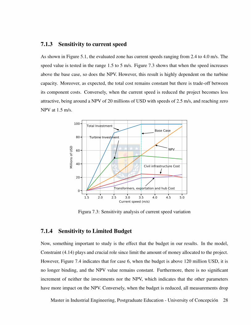
7.1.3 Sensitivity to current speed

As shown in Figure 5.1, the evaluated zone has current speeds ranging from 2.4 to 4.0 m/s. The

speed value is tested in the range 1.5 to 5 m/s. Figure 7.3 shows that when the speed increases

above the base case, so does the NPV. However, this result is highly dependent on the turbine

capacity. Moreover, as expected, the total cost remains constant but there is trade-off between

its component costs. Conversely, when the current speed is reduced the project becomes less

attractive, being around a NPV of 20 millions of USD with speeds of 2.5 m/s, and reaching zero

NPV at 1.5 m/s.

1.5 2.0 2.5 3.0 3.5 4.0 4.5 5.0Current speed (m/s)

0

20

40

60

80

100

Milli

ons o

f USD

Total Investment

NPV

Turbine Investment



Base Case

Figura 7.3: Sensitivity analysis of current speed variation

7.1.4 Sensitivity to Limited Budget

Now, something important to study is the effect that the budget in our results. In the model,

Constraint (4.14) plays and crucial role since limit the amount of money allocated to the project.

However, Figure 7.4 indicates that for case 6, when the budget is above 120 million USD, it is

no longer binding, and the NPV value remains constant. Furthermore, there is no significant

increment of neither the investments nor the NPV, which indicates that the other parameters

have more impact on the NPV. Conversely, when the budget is reduced, all measurements drop


with less intensity when compared to the other parameters. Thus, a reduction of 60% in budget

produces a reduction of around 50% in NPV.

40 50 60 70 80 90 100 110 120Budget (MUSD)

0

20

40

60

80

100

120M

illion

s of U

SDTotal Investment

NPV

Turbine Investment



Base Case

Figura 7.4: Sensitivity analysis of limited budget

Additionally, it was investigated how the TCF design is affected when the budget is increased in

case 10 to 170 and 200 MUS$. Figure 7.5 depicts both TCFs layouts, where it can be observed

they have a similar structure, and the TCTs are placed in such a way that the wake effect is

reduced. Finally, the problems become more difficult to solve as the budget increases. The gap

value remains in an acceptable level (under 14%) considering the large-sized of case 10, but this

gap could be reduced if more time is allocated to run the model.


◦ • ◦ ◦ ◦ ◦ ◦ ◦ ◦ ◦ ◦ ◦ ◦ ◦ ◦• ◦ ◦ ◦ ◦ ◦ ◦ ◦ ◦ ◦ ◦ ◦ ◦ ◦ ◦• ◦ ◦ ◦ ◦ ◦ ◦ • ◦ ◦ ◦ ◦ ◦ ◦ ◦◦ • ◦ ◦ ◦ ◦ ◦ ◦ ◦ ◦ ◦ ◦ ◦ ◦ ◦◦ • ◦ ◦ ◦ • ◦ ◦ ◦ ◦ ◦ ◦ ◦ ◦ ◦• ◦ ◦ • ◦ ◦ ◦ ◦ ◦ ◦ ◦ ◦ ◦ ◦ ◦• ◦ ◦ • ◦ ◦ ◦ ◦ ◦ ◦ ◦ ◦ ◦ ◦ ◦◦ ◦ • ◦ ◦ ◦ ◦ ◦ ◦ ◦ ◦ ◦ ◦ ◦ ◦

⊗ ◦ • ◦ ◦ ◦ ◦ ◦ ◦ ◦ ◦ ◦ ◦ ◦ ◦ ◦◦ ◦ ◦ • ◦ • ◦ ◦ ◦ ◦ ◦ ◦ ◦ ◦ ◦◦ ◦ ◦ ◦ ◦ • ◦ ◦ ◦ ◦ ◦ ◦ ◦ ◦ ◦• ◦ ◦ ◦ ◦ ◦ ◦ ◦ ◦ • ◦ ◦ ◦ ◦ ◦◦ ◦ ◦ ◦ ◦ ◦ • ◦ ◦ ◦ ◦ ◦ ◦ ◦ ◦◦ • ◦ ◦ ◦ ◦ ◦ ◦ ◦ ◦ ◦ ◦ ◦ ◦ ◦◦ • ◦ • ◦ ◦ ◦ ◦ ◦ ◦ ◦ ◦ ◦ ◦ ◦◦ ◦ • ◦ ◦ • ◦ ◦ ◦ ◦ ◦ ◦ ◦ ◦ ◦

(a) Case 10 with B=170 and 24 turbines.

◦ • ◦ ◦ ◦ ◦ ◦ ◦ ◦ ◦ ◦ ◦ ◦ ◦ ◦• ◦ ◦ ◦ • ◦ ◦ ◦ ◦ ◦ ◦ ◦ ◦ ◦ ◦◦ • ◦ ◦ ◦ • ◦ ◦ ◦ ◦ ◦ ◦ ◦ ◦ ◦◦ • ◦ ◦ • ◦ ◦ ◦ ◦ ◦ ◦ ◦ ◦ ◦ ◦◦ ◦ ◦ ◦ ◦ ◦ ◦ ◦ ◦ • ◦ ◦ ◦ ◦ ◦• ◦ ◦ • ◦ ◦ ◦ • ◦ ◦ ◦ ◦ ◦ ◦ ◦◦ ◦ ◦ • ◦ ◦ ◦ ◦ ◦ ◦ ◦ ◦ ◦ ◦ ◦• ◦ • ◦ ◦ • ◦ ◦ ◦ ◦ ◦ ◦ ◦ ◦ ◦

⊗ ◦ • ◦ ◦ ◦ ◦ ◦ ◦ ◦ ◦ ◦ ◦ ◦ ◦ ◦◦ ◦ ◦ ◦ ◦ • ◦ ◦ ◦ ◦ ◦ ◦ ◦ ◦ ◦◦ ◦ ◦ ◦ ◦ • ◦ • ◦ ◦ ◦ ◦ ◦ ◦ ◦◦ ◦ ◦ ◦ ◦ ◦ ◦ • ◦ • ◦ ◦ ◦ ◦ ◦◦ ◦ • ◦ ◦ ◦ • ◦ ◦ ◦ ◦ ◦ ◦ ◦ ◦◦ ◦ • ◦ ◦ ◦ ◦ ◦ ◦ ◦ ◦ ◦ ◦ ◦ ◦◦ ◦ • ◦ ◦ ◦ ◦ ◦ ◦ • ◦ ◦ ◦ ◦ ◦◦ ◦ • ◦ ◦ • ◦ ◦ ◦ ◦ ◦ ◦ ◦ ◦ ◦

(b) Case 10 with B=200 and 28 turbines.

⊗ : Hub Collector, • : Turbines Installed

◦ : Unused Nodes, : Electrical cables

Figura 7.5: Cases to increase the budget


7.2. Comparison with literature

The methodology presented in this work has been applied through the case study presented

above, to verify its performance. The results obtained make it possible to establish that the pro-

posed optimization model not only solves the problem raised but also has advantages compared

to what is stated in the literature. Among the observations made to the routing models, it is

noted that there are both limitations by the size of the problem (Fagerfjall (2010), Pillai et al.

(2015), Fischetti and Pissinger (2018b) as for the consideration of energy losses (Srikalapu and

U (2017)). This model can solve problems with cases greater than 200 nodes in times that are

considered acceptable. It is true that runtime of 10.800 seconds, in the case 10, can be consid-

ered a long time to get results. However, it is necessary to say that the model is only run once,

unlike other models that must be run several times depending on the problem they solve. In

this case, the feasibility assessment is performed at the start of the project, not having to run the

programmed model a second time.

This methodology stands out for the resolution of layout optimization and cable routing problem

in the same model. This means a more practical procedure compared to other OWF models. The

papers related to cable routing problem solve cases composed of pre-designed. In most cases,

cable routing is done over existing plant layouts, while other works use computer-simulated

layouts. In this work, the proposed model generates a layout from the input data, and at the

same time solves cable routing. The layout delivered by the model is considered feasible, as

it is generated from actual data of the speed and bathymetry of the Chacao Canal, in addition

to the calculation of the power generated and the losses by the effect of wake and transmission

in electrical lines. Moreover, authors such as Herrera Hernandez (2010) and Galloway et al.

(2014), have proposed TCF with layouts similar to the design obtained by the MIP.

About layout optimization for TCF presented in the literature papers, this model performs a bet-

ter way. The methodology used in this work is based on an optimization model solved by an


exact algorithm, which guarantees an optimal solution. Although the use of algorithms deter-

mines the robustness of the procedure, it does not guarantee optimal solutions due to its iterative

process, along with the two-phase resolution that the algorithm needs to be executed. This adds

to the model presented by both Funke et al. (2013) as by Culley et al. (2016) is of a nonlinear

type, which further complicates the search for optimal solutions. This work performs well when

solving large cases (greater than 100 nodes) while the algorithm proposed by OpentidalFarm

can only solve a limited number of nodes,

7.3. Insights

The main insights obtained from the results mentioned above are:

• The proposed methodology is easy to adapt and can be implemented using commercial

MIP software.

• This methodology can be extended to incorporate other features and opens new possibili-

ties for the fast evaluation of TCF projects.

• Geographical information systems (GIS) and mixed-integer programming models can be

used to design and evaluate TCF projects.

• An investment of 146.608 MUS$ in a TCF of 60.45 MW would generate 219 GWh of

energy annually, sufficient to supply power to the entire population of Chiloe island in

Chile.

• Current speeds higher than 2.5 m/s are recommended for an economically viable TCF

project.

• Small changes on the budget do not have a significant impact on the NPV of a TCF project.

• In Chile, a minimum of 40 US$/MWh price is advised to consider a TCF project profitable.

Even though an interval of 30-40 US$/MWh still produces a positive NPV, it could be too

risky from abrupt changes in the model parameters.


• With an opportunity cost higher than 9%, the TCF project becomes less attractive. Be-

sides, a discount rate of less than 6% seems advisable to ensure good returns of the TCF

project.

Finally, this study is limited by the wake model that has been used. The Jensen’s wake model

is a realistic way to observe the behavior of the wake. However, it does not consider the direct

effects of fluid viscosity, as well as variations in turbulence and wake regimens. Moreover, this

work only considers the effect of wake strictly in the downstream direction. Another limitation

of this work is that current speeds were measured in sections of 50-100 meters, which means

lower accuracy in the analysis of losses. But the low measurement accuracy does not change the

behavior of the results, which are according to those proposed by the technical literature.


Chapter 8. Conclusions

The importance of an optimal configuration of a TCF project has been discussed and a method-

ology for the overall design and evaluation of a TCF has been introduced. This model allows

obtaining both the layout of turbines optimally and the best array of the electrical connection

between the devices. For this work, Jensen’s wake effect Model was used to determine the be-

havior of the wake and its influence on the turbine location. The proposed model performs an

economic evaluation of the project considering a useful life of 20 years, thus determining the

profitability of a TCF. This model was solved by an accurate algorithm method, in acceptable

computational times.

A case study was considered to determine the feasibility of the model. This consisted of a TCF

ideally located in the Chacao Canal, Chile. Cases were solved to determine the effectiveness of

the model, based on the size of the TCF. Besides, the behavior of the optimal solution is com-

piled according to the variation of some important parameters.

For future work, it is recommended to explore the use of new methodologies that study the

effects of wake. More accurate consideration of certain physical characteristics of tides, such

as viscosity or turbulence regimes, will result in more complete and realistic results. The new

approaches will allow the study of new possibilities to implement projects of this kind, which

help the environment and improve the quality of life of people.


References

Aguayo, M. M., Sarin, S. C., and Sherali, H. D. (2018). Solving the single and multiple asym-

metric traveling salesmen problems by generating subtour elimination constraints from inte-

ger solutions. IISE Transactions, 50(1):45–53.

Amaral, L. and Castro, R. (2017). Offshore wind farm layout optimization regarding wake

effects and electrical losses. Engineering Applications of Artificial Intelligence, 60(0):26–34.

Bauer, J. and Lysgaard, J. (2015). The offshore wind farm array layout problem: A planar open

vehicle routing problem. Journal of the Operational Research Society, 66(3):360–368.

Culley, D., Funke, S., Kramer, S., and Piggot, M. (2016). Integration of cost modelling within

the micro-setting design optimization of tidal turbine arrays. Renewable Energy, 85(3):215–

227.

Dai, Y., Ren, Z., Wang, K., and Li, W. (2017). Optimal sizing and arrangement of tidal current

farm. IEEE Trans. Power Syst., pages 1–10.

Fagerfjall, P. (2010). Optimizing Wind Farm Layout - More Bang fot the Buck Using Mixed In-

teger Linear Programming. Master’s thesis. Chalmers University of Technology and Gothen-

burg University.

Fischetti, M. and Pisinger, D. (2017). Optimizing wind farm cable routing considering power

losses. European Journal of Operational Research, 14(3):223–259.

Fischetti, M. and Pisinger, D. (2018a). Mixed integer linear programming for new trends in

wind farm cable routing. Electronic Notes in Discrete Mathematics, 64(3):115–124.

Fischetti, M. and Pisinger, D. (2018b). On th impact of considering power losses in offshore

wind farm cable routing. European Journal of Operational Research, 20(3):220–245.

Funke, S., Farrell, P., and Piggot, M. (2013). Tidal turbine array optimisation using the adjoint

approach. Renewable Energy, 63:658–673.


Funke, S., Kramer, S., and Piggot, M. (2016). Design optimisation and resource assessment for

tidal-stream renewable energy farms using a new continuous turbine approach. Renewable

Energy, 99:1046–1061.

Galloway, P., Myers, L., and Bahaj, A. (2014). Quantifying wave and yaw effects on a scale

tidal stream turbine. Renewable Energy, 63(3):297–307.

Gong, X., Kuenzel, S., and Pal, B. (2017). Optimal wind farm cabling. IEEE System Journal,

10(1):20–30.

Gonzalez-Longatt, F., Wall, P., Reguinski, P., and Terzija, V. (2012). Optimal electric network

design for a large offshore wind farm based on a modified genetic algorithm approach. IEEE

System Journal, 6(1):164–172.

Guerra, M., Cienfuegos, R., Thomson, J., and Suarez, L. (2017). Tidal energy resource charac-

terization in chacao channel, chile. International Journal of Marine Energy, 20(6):1–16.

Hassan, G. (2009). Preliminary Site Selection - Chilean Marine Energy Resource. Garrad

Hassan and Partners Limited.

Herrera Hernandez, R. (2010). Technical-economic feasibility analysis of the energy resource

associated with tidal currents in the Chacao channel. Civil Engineering Department, Univer-

sity of Chile.

IRENA (2014). Ocean energy technology: readiness, patents and deployment status and out-

look. Technical Report, European Wind Energy Association.

Ituarte-Villarreal, C. and Espiritu, J. (2011). Optimization of wind turbine placement using a

viral based optimization algorithm. Pocedia Computer Science, 6(0):469–474.

Jayasinghe, K. (2017). Power Loss evaluation of submarine cables in 500mW offshore wind

farm. Erath Science Department, Uppsala University.


Jensen, N. (1983). A note of wind generator interaction. Riso National Library, Roskilde,

Denmark.

Klein, A. and Haugland, D. (2017). Obstacle.aware optimization of offshore wind farm cable

layouts. Advantages in theorical and applied combinatorial, 5(1):100–116.

Kramer, S., Funke, S., and Piggot, M. (2016). A continuous approach for the optimisation of

tidal turbine farms. European Wave and Tidal Energy Conference 2015.

Kuo, J., Romero, D., and Amon, C. (2015). A mechanistic semi-empirical wake interaction

model for wind farm layout optimization. Energy, 93(3):2157–2165.

Lumbreras, S. and Ramos, A. (2011). A bender’s decompotition approach for optimizing the

electric system of offshore wind farm. IEEE Trodheim, 1(1):1–8.

Lumbreras, S. and Ramos, A. (2013). Optimal design of the electrical layout of an offshore

wind farm applying descomposition strategies. IEEE Trans. Power Syst., 28(2):1434–1441.

Neill, S., Angeloudis, A., Robins, P., Walkington, I., Ward, S., Masters, I., Lewis, M., Piano,

M., Avdis, P., Aggidis, G., Evans, P., Adcock, T., Zidonis, A., Ahmadian, R., and Falconer,

R. (2018). Tidal range energy resource and optimization - past persepective and future chal-

lenges. Renewable Energy, 127(3):763–778.

Pillai, A., Chick, J., Khorasanchi, and Johannig, L. (2016). Optimisation of offshore wind farms

using genetic algorithm. International Journal of Offshore and Polar Engineering, 26(3):225–

234.

Pillai, A., Chick, J., Khorasanchi, M., Barbouchi, S., and Johannig, L. (2017). Application of

an offshore wind farm layout optimization methodology at middelgrunden wind farm. Ocean

Engineering, 139(10):297–287.

Pillai, A., Chick, J., Khorasanchi, M., and de Laleu, V. (2015). Offshore wind farm electrical

cable layout optimization. Engineering Optimization, 30(10):1–20.


Quinonez-Varela, G., Ault, G., Anaya-Lara, O., and McDonald, J. (2007). Electrical collectors

system options for a large offshore wind farms. Power Gener IET, 1(2):107–114.

Rodrigues, S., Bosman, P., and Bauer, P. (2016a). Multi-objective optimization of wind layouts-

complexity, constraints handing and scalability. Renewable and sustainable energy reviews,

65(20):587–608.

Rodrigues, S., Restrepo, C., Katsouris, G., Texeira, R., Bosman, P., Bauer, P., and Soleiman-

zadeh, M. (2016b). A multi-objective optimization framework for offshore wind farm layouts

and electric infrastructures. Energies, 11(1):5–47.

Segura, E., Morales, R., and Somolinos, J. (2017). Cost assessment methodology and economic

viability of tidal energy projects. Energies, 10(3):1–27.

Serrano Gonzalez J, Gonzalez Rodrıguez, G., Castro Mora, J., Riquelme Santos, J., and Bur-

gos Payan, M. (2010). Optimization of wind farm turbines layout using an evolutive algo-

rithm. Renewable Energy, 35(8):1671–1681.

Shin, J.-S. and Kim, J.-O. (2016). Optimal design of offshore wind farm considering inner grid

layout and offshore substation location. IEEE System Journal, 10(2):90–99.

Srikakulapu, R. and U, V. (2017). Combined approach based on aco with mtsp for optimal in-

ternal electrical system design of large offshore wind farm. Journal of Modern Power System

and Clean Energy, 40(4):100–112.

Turner, S., Romero, D., Zhang, P., Amon, C., and Chan, T. (2014). A new mathematical pro-

gramming approach to optimize wind farm layouts. Renewable Energy, 63(3):674–680.

Vartdal, J., Qassi, R. Y., Monkliev, Borge, a. U. G., and Gonzalez-Gorbena, E. (2018). Opti-

mal configuration problem identification of electrical power cable in tidal turbine farm via

traveling salesman problem modeling approach. Journal of Modern Power System and Clean

Energy, 45(4):165–172.


Villalon, V., Watts, D., and Cienfuegos, R. (2019). Assessment of the power potential extraction

in the chilean chacao channel. Renewable Energy, 131(6):585–596.

Wade, B., Pereira, R., and Wade, C. (2019). Investigation of oofshore wind farm layouts regard-

ing wake effects and cable topology. Journal of Physics, 122(4):120–141.

Wedzik, A., Siewerski, T., and Szypowski, M. (2016). A new method for simultaneous opti-

mizing of wind farm’s network layout and cable cross-sections by milp optimization. Applied

Energy, 182(4):525–538.

Zuo, T., Meng, K., Tong, Z., Tang, Y., and Dong, Z. (2018). Offshore wind farm collector

system layout optimization based on self-tracking minimum spanning tree. Int Trans Electr

Energ Syst., pages 1–16.


Documents

UNIVERSITY OF CONCEPCION - CHILE FACULTY OF …