UNIVERSITY OF CINCINNATI - UCFileSpace Tools - Homehomepages.uc.edu/~maynarjb/Frontpage sites/Research/s/Ada… · B.S. University of Cincinnati ... The Simco wetland was flooded

UNIVERSITY OF CINCINNATI

_____________ , 20 _____

I,______________________________________________,hereby submit this as part of the requirements for thedegree of:

________________________________________________

in:

________________________________________________

It is entitled:

________________________________________________

________________________________________________

________________________________________________

________________________________________________

Approved by:________________________________________________________________________________________________________________________

Sulfate Reduction In Five Constructed Wetlands Receiving Acid Mine Drainage

A Thesis submitted to the

Division of Research and Advanced Studies of the University of Cincinnati

in partial fulfillment of the

requirement for the degree of

MASTER OF SCIENCE

In the Department of Geological Sciences of the College of Arts and Sciences

2001

by:

Adam Flege

B.S. University of Cincinnati

Committee Chair: Dr. J. Barry Maynard

Committee Members: Dr. David Nash, Dr. Jodi Shann

Abstract

Constructed wetlands have been shown to be effective in treating various types of

wastewater. One type, Acid Mine Drainage (AMD), is characterized by high acidity,

heavy metals, and sulfate. Five Constructed Wetlands, Friar Tuck, Tecumseh, and

Midwestern in southwestern Indiana, and Simco and Wills Creek wetland in Ohio, were

studied to determine their treatment efficiencies for sulfate and metal removal. Sulfate

Reduction by microorganisms in constructed wetlands can remove sulfate and dissolved

metals, and can generate alkalinity. Approximately 100 water samples and 50 soil

samples were taken during the winter and summer seasons at the five wetlands and

analyzed for sulfate and metal concentrations, sulfur isotope values, pH, Eh, and

conductivity. Resulting data indicates that sulfate reduction is occurring at all five

wetlands, but varies in degrees of treatment effectiveness. The Friar Tuck wetland shows

minimal evidence of sulfate reduction, with dilution being the main remediation

mechanism. A small volume of AMD is being overwhelmed by numerous freshwater

inputs resulting in a significant improvement in water chemistry due to this dilution. The

Tecumseh wetland shows little change in influent/effluent sulfate and sulfide values

suggesting that treatment of the influent wastewater by sulfate reduction was ineffective

for both sampling seasons. The Midwestern wetland for the summer season shows a

significant increase in water sample δ34S, from -5.03 permil to +0.27 permil with a

corresponding drop in sulfate concentrations from 1740 ppm to 831 ppm, demonstrating

successful sulfate reduction and wastewater treatment. However, the winter season

sampling showed no change in δ34S, indicating only minor sulfate reduction, but sulfate

concentrations still fell from 1740 ppm to 831 ppm, indicating an additional sulfate

removal process. The Wills Creek wetland shows little change in influent/effluent sulfate

concentrations and sulfur isotope values suggesting that sulfate reduction is inactive for

both sampling seasons. The Simco wetland was flooded due to beaver constructed damns

during our winter sampling and accurate data were not obtained. Summer water sample

data show a significant increase in δ34S, from –3.58 at the influent to +6.26 at the effluent

and a corresponding decrease in sulfate concentrations from 640 ppm to 290 ppm,

demonstrating successful sulfate reduction trends.

Acknowledgments There are many people that deserve my undying thanks and appreciation for

support on a project that never seemed to end. A big thank you goes out to: Barry

Maynard, my advisor, for his help with sampling, writing, funding, and so many other

things that there’s not enough space to mention it all. Dr. David Nash and Dr. Jodi

Shann, who sat on my committee and offered advice to better the project. Dr. Erika

Elswick, who took time to help organize and arrange time for lab work at Indiana

University. Steve Studley at Indiana University for his help in the Mass Spectrometer

lab. My mother and father, Eileen and Frank, who have been nothing but supportive and

caring throughout this whole process. Without them, I wouldn’t have finished and

wouldn’t be where I am today, and I wouldn’t have had a place to stay during the entire

experience. My fiance Erin, who by the time you read this will be my wife, was always

there to remind of me of the direction I needed to go and to encourage me throughout all

the times I just wanted to hang it up. My future parent in laws Peter and Joy, who kept

me fed and welcomed me openly into their home and family. Mikes Nicholis, for sharing

an office and offering ideas and opinions that undoubtedly influenced the final product

for the better. All of the “Rays” for keeping me sane, making me laugh and taking my

mind off intimidating deadlines and incomplete manuscripts. All of my friends from

undergrad who influenced me to try for a masters. Stacy, for keeping me positive with

emails of encouragement, all the way from Oregon. Cindy, for being there to talk to

when things got a little too rocky. Ryan, for keeping me on my toes and always making

me smile with his shinanigans. I would also like to thank the Indiana Division of

Reclamation for their financial support of the project and Indiana University Department

of Geological Sciences for their laboratory support.

1

Table of Contents List of Figures 3 List of Tables 6 List of Appendices 7 Chapter 1 – Introduction to Constructed Wetlands, Acid Mine Drainage, and

Sulfate Reduction 8 1.1 History of Acid Mine Drainage and Its Effect on the Environment 8 1.2 Conventional AMD Chemical Treatment 9 1.3 Use of Constructed Wetlands to Treat AMD Wastewater 10 1.4 Anoxic Limestone Drains in Constructed Wetlands 11 1.5 Design and Sizing of Constructed Wetland Cells 12 1.6 Wetland Cell Substrate 13 1.7 Sulfate Reduction 14 1.8 Use of Sulfur Isotopes to Determine the Efficiency of

Sulfate Reduction 16 Chapter 2 – History of Wetlands Studied 17

2.1 Friar Tuck Wetland 19 2.2 Tecumseh Wetland 21 2.3 Midwestern Wetland 23 2.4 Wills Creek Wetland 26 2.5 Simco Wetland 31

Chapter 3 – Analytical Methods 34

3.1 Introduction 34 3.2 Dissolved Sulfate 34 3.3 Sulfides 35 3.4 Porewater Sulfides and Samples 38 3.5 Sulfur Isotopes 39 3.6 %Carbon - %Sulfur 40 3.7 Sediment Mineralogy 40 3.8 Bulk Chemistry 40 3.9 PHREEQC 41

Chapter 4 – Results and Interpretation 42

4.1 Friar Tuck Wetland 42 4.1.1 Introduction 42 4.1.2 Soil Samples 43 4.1.3 Water Samples 43 4.1.4 Conclusion 45

4.2 Tecumseh Wetland 51 4.2.1 Introduction 51 4.2.2 Sampling 53 4.2.3 Water Samples 55

4.2.3.1 Field Measurements 55

2

4.2.3.2 Sulfate Concentrations 55 4.2.3.3 Sulfur Isotopes 57 4.2.3.4 Metal Concentrations 59

4.2.4 Soil Samples 59 4.2.5 Conclusion 61

4.3 Midwestern Wetland 70 4.3.1 Introduction 70 4.3.2 Sampling 72 4.3.3 Water Samples 73

4.3.3.1 Field Measurements 73 4.3.3.2 Sulfate Concentrations 74 4.3.3.3 XRD Samples 75 4.3.3.4 Sulfur Isotopes 76 4.3.3.5 Metal Concentrations 77


4.4 Wills Creek Wetland 88 4.4.1 Introduction 88 4.4.2 Sampling 90 4.4.3 Water Samples 91

4.4.3.1 Field Measurements 91 4.4.3.2 Sulfate Concentrations 91 4.4.3.3 Sulfur Isotopes 92 4.4.3.4 Metal Concentrations 93


4.5 Simco Wetland 101 4.5.1 Introduction 101 4.5.2 Sampling 103

4.5.2.1 Past Sampling and Interpretation 104 4.5.3 Water Samples 105

4.5.3.1 Field Measurements 105 4.5.3.2 Sulfate Concentrations 106 4.5.3.3 Sulfur Isotopes 106 4.5.3.4 Metal Concentrations 107


Chapter 5 – Discussion 117 5.1 Wetland Sizing and Design 117 5.2 Anoxic Limestone Drains 118 5.3 Water Samples and Soil Samples 120 5.4 Sulfate Reduction 121 5.5 Recommendations for Future Study 122 Chapter 6 – References 124

3

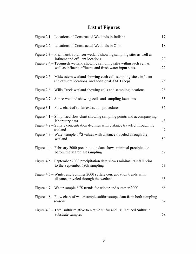
List of Figures Figure 2.1 – Locations of Constructed Wetlands in Indiana 17 Figure 2.2 – Locations of Constructed Wetlands in Ohio 18 Figure 2.3 – Friar Tuck volunteer wetland showing sampling sites as well as

influent and effluent locations 20 Figure 2.4 – Tecumseh wetland showing sampling sites within each cell as

well as influent, effluent, and fresh water input sites. 22 Figure 2.5 – Midwestern wetland showing each cell, sampling sites, influent

and effluent locations, and additional AMD seeps 25 Figure 2.6 – Wills Creek wetland showing cells and sampling locations 28 Figure 2.7 – Simco wetland showing cells and sampling locations 33 Figure 3.1 – Flow chart of sulfur extraction procedures 36 Figure 4.1 – Simplified flow chart showing sampling points and accompanying

laboratory data 48 Figure 4.2 – Sulfate concentration declines with distance traveled through the

wetland 49 Figure 4.3 – Water sample δ34S values with distance traveled through the

wetland 50 Figure 4.4 – February 2000 precipitation data shows minimal precipitation

before the March 1st sampling 52 Figure 4.5 – September 2000 precipitation data shows minimal rainfall prior

to the September 19th sampling 53 Figure 4.6 – Winter and Summer 2000 sulfate concentration trends with

distance traveled through the wetland 65 Figure 4.7 – Water sample δ34S trends for winter and summer 2000 66 Figure 4.8 – Flow chart of water sample sulfur isotope data from both sampling

seasons 67 Figure 4.9 – Total sulfur relative to Native sulfur and Cr Reduced Sulfur in

substrate samples 68

4

Figure 4.10 – Native Sulfur and Cr Reduced Sulfur δ34S values with distance traveled through the wetland 69

Figure 4.11 – February 2000 precipitation data shows minimal precipitation before the March 1st sampling 71

Figure 4.12 – September 2000 precipitation data shows minimal precipitation prior to the September 18th sampling 71

Figure 4.13 – Winter and Summer 2000 and Winter 2001 sulfate concentration

trends with distance traveled through the wetland 84 Figure 4.14 – Flow chart of water sample sulfur isotope data from all three

sampling seasons 85 Figure 4.15 – Change in water sample isotope values for winter and summer

2000 and winter 2001 with distance traveled through the wetland 86 Figure 4.16 – Native Sulfur isotope values for soil samples from 3/1/00 and

9/18/00 versus distance traveled through the wetland 87 Figure 4.17 – March 2000 precipitation data shows no precipitation prior to

the March 9th sampling 89 Figure 4.18 – August 2000 precipitation data shows significant rainfall the

day of sampling, affecting residence times and discharge calculations 90

Figure 4.19 – Sulfate concentration trends with distance traveled through the

wetland 97 Figure 4.20 – Water sample sulfur isotope values with distance traveled

through the wetland 98 Figure 4.21 – Flow chart of water sample sulfur isotope data for both sampling

seasons 99 Figure 4.22 – Native Sulfur and Cr Reduced Sulfur isotopes for winter and

summer seasons versus distance traveled through the wetland 100 Figure 4.23 – May 2000 precipitation data shows minimal precipitation before

the May 11th sampling 102 Figure 4.24 – August 2000 precipitation data shows significant rainfall the

day of sampling, affecting residence times and discharge calculations 103

5

Figure 4.25 – Sulfate concentration trends for winter and summer 2000 and winter 2001 with distance traveled through the wetland 113

Figure 4.26 – Flow chart of water sample sulfur isotope data for all three

sampling seasons 114

Figure 4.27 – Water sample sulfur isotopes for all seasons versus distance traveled through the wetland 115

Figure 4.28 – Native Sulfur isotope values versus distance traveled through

the wetland 116 Figure 5.1 – Substrate samples show minimal correlation when compared with

water samples 121

6

List of Tables Table 1 – Wills Creek past sampling data 30 Table 2 – Friar Tuck water and soil samples taken 2/29/00 47 Table 3 – Tecumseh water samples taken for winter and summer seasons 62 Table 4 – Tecumseh water sample sulfur isotope and sulfate concentration data 63 Table 5 – Tecumseh influent and effluent metal concentrations 63 Table 6 – Tecumseh soil sample and sulfur isotope and % sulfur data 64 Table 7 – Midwestern water samples taken 3/1/00 and 9/18/00 80 Table 8 – Midwestern water samples taken 2/23/01 81 Table 9 – Midwestern water sample sulfur isotope and sulfate concentration data 82 Table 10 – Midwestern influent and effluent metal concentrations 83 Table 11 – Midwestern soil sample sulfur isotope and % sulfur data 83 Table 12 – Wills Creek water samples taken 3/1/00 and 9/18/00 95 Table 13 – Wills Creek water sample sulfur isotope and sulfate

concentration data 95 Table 14 – Wills Creek influent and effluent metal concentrations 96 Table 15 – Wills Creek soil sample sulfur isotope and % sulfur data 96 Table 16 – Simco past sampling data 104 Table 17 – Simco water samples taken all three seasons 110 Table 18 – Simco water sample sulfur isotope and sulfate concentration data 111 Table 19 – Simco influent and effluent metal concentrations 111 Table 20 – Simco soil sample sulfur isotope and % sulfur data 112

7

List of Appendices Appendix A – Weight % Carbon and Sulfur 128 Appendix B – X-ray Fluorescence Data 130 Appendix C – Wet Chemistry / Metal Concentration Data 132 Appendix D – X-ray Diffractogram Data 134 Appendix E – PHREEQC Analysis 146

8

Chapter 1: Introduction to Acid Mine Drainage and Sulfate Reduction

1.1 History of Acid Mine Drainage and Its Effect on the Environment

Ever since the beginning of coal mining, companies have been faced with a

variety of related pollution problems. Most problems today are closely monitored and

regulated by both state and federal agencies in order to protect the environment and

public health. The Surface Mining Control and Reclamation Act of 1977 set the rules for

the regulation of all coal mining activities within the United States. This, and other laws,

ensure that all mined lands will be reclaimed, that the biological integrity of the area is

maintained, and that other resources will not be degraded due to mining (Eddy 1995).

Acid Mine Drainage (AMD), which contains a number of dissolved metals including

Manganese (Mn) and Iron (Fe), is one of the major problems resulting from coal mining.

AMD is created by the interaction of air and water with sulfides, mainly pyrite (FeS2),

found in overburden piles consisting of sub-commercial grade mining material left over

from the mining process. Pyrite in the overburden is oxidized via the following chemical

process (Hsu and Maynard 1999):

FeS2 + 7/2O2 + H2O Fe2+ + 2SO42- + 2H+

Fe2+ + H+ + 1/4O2 Fe3+ + 1/2H2O

Fe3+ + 3H2O Fe(OH)3 + 3H+

9

In equation 1, pyrite oxidizes into iron sulfate (FeSO4) and sulfuric acid (H2SO4). Pyrite

can also be oxidized in an anoxic environment by the following reaction (Stumm and

Morgan, 1981):

FeS2 + 14 Fe3+ + 8H2O 15Fe2+ + 2SO42- + 16H+

The oxidizer in equation 2 is ferric iron (Fe3+), which can be supplied by the reactions in

equation 1. Thus, once the oxidation of pyrite begins, the process can continue regardless

of the presence of oxygen.

The result is a solution of low pH with a high concentration of dissolved metals

and sulfate. This drainage flows into local streams, lakes, and rivers, contaminating soils

and destroying plant and animal biotas. Smith (1989) and Kleinman (1989) estimated

that over 12,000 miles of rivers and streams and over 180,000 acres of lakes and

reservoirs in the U.S. have been affected by AMD. Control of where AMD goes is of the

utmost importance to mine owners since legal responsibility could fall on their shoulders

for any damage resulting from their activities. Thus, owners of mining operations treat

the effluent AMD before it becomes a financial liability or an environmental threat.

1.2 Conventional AMD Chemical Treatment

Conventional treatment involves AMD being pumped to a central location where

it is treated with a variety of costly chemicals including caustic soda, sodium hydroxide,

potassium hydroxide, and soda ash. Adding these alkaline materials increases the pH of

the effluent to between 9 and 11 (Kleinman 1989), sufficient to cause the precipitation of

10

metal oxides. The Federal Clean Water Act of 1977 requires that effluent waters from

coal mining areas have a total 30-day discharge Fe and Mn concentration of <3.5 mg/L

and <2 mg/L respectively and maintain a pH between 6 and 9 (Stark et al. 1990). The

conventional chemical treatment process is fairly successful at achieving these discharge

standards. However, since AMD can remain a problem for many years, chemical

treatment can become financially staggering, with estimated costs to the mining industry

of over $1 million a day (Kleinmann 1989). Clearly, a cheaper, more efficient method of

AMD treatment would be desirable.

1.3 Use of Constructed Wetlands to Treat AMD Wastewater

Constructed wetlands are one method used for the passive treatment of AMD.

The ability of wetlands to improve water quality was identified in the late 1970’s and

since then, hundreds of wetlands have been constructed for the sole purpose of treating

AMD (Eddy 1995). Reclaimed strip mine land and land surrounding subsurface mines

were graded to channel surface and subsurface runoff into a constructed wetland.

Chemical and biological processes within the wetland act to improve water quality.

However, designs for these early wetlands were not well planned and many of them

failed after only a few short years. Several factors are required for a wetland to continue

to operate efficiently and maintain successful operation over a long period of time. In

order to understand which factors contribute to a successful wetland and which ones do

not, it is important to first understand the design principles behind how a wetland is

constructed and how each particular aspect of a wetland works. A typical wetland design

uses multiple cells through which AMD travels. Flow from cell to cell is controlled by

11

weirs and flow within cells is often controlled and channeled by berms built into the

middle of the cells. Most wetland designs use an anoxic limestone drain (ALD) to

increase the pH of influent AMD into the system.

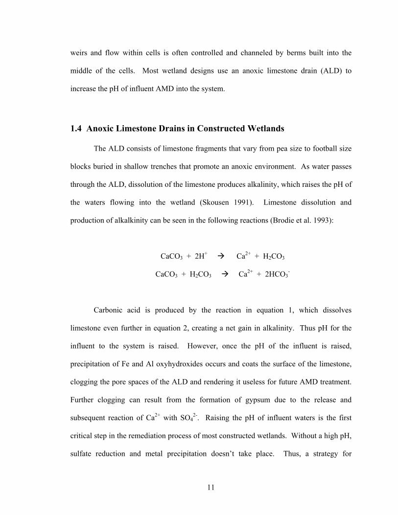
1.4 Anoxic Limestone Drains in Constructed Wetlands

The ALD consists of limestone fragments that vary from pea size to football size

blocks buried in shallow trenches that promote an anoxic environment. As water passes

through the ALD, dissolution of the limestone produces alkalinity, which raises the pH of

the waters flowing into the wetland (Skousen 1991). Limestone dissolution and

production of alkalkinity can be seen in the following reactions (Brodie et al. 1993):

CaCO3 + 2H+ Ca2+ + H2CO3

CaCO3 + H2CO3 Ca2+ + 2HCO3-

Carbonic acid is produced by the reaction in equation 1, which dissolves

limestone even further in equation 2, creating a net gain in alkalinity. Thus pH for the

influent to the system is raised. However, once the pH of the influent is raised,

precipitation of Fe and Al oxyhydroxides occurs and coats the surface of the limestone,

clogging the pore spaces of the ALD and rendering it useless for future AMD treatment.

Further clogging can result from the formation of gypsum due to the release and

subsequent reaction of Ca2+ with SO42-. Raising the pH of influent waters is the first

critical step in the remediation process of most constructed wetlands. Without a high pH,

sulfate reduction and metal precipitation doesn’t take place. Thus, a strategy for

12

recharging or replacing the ALDs of constructed wetlands with fresh limestone riprap

would perpetuate the life of the wetland. However, the goal of constructed wetlands is to

keep maintenance costs to a minimum, and repeated recharging of ALDs would

significantly increase operational expenses.

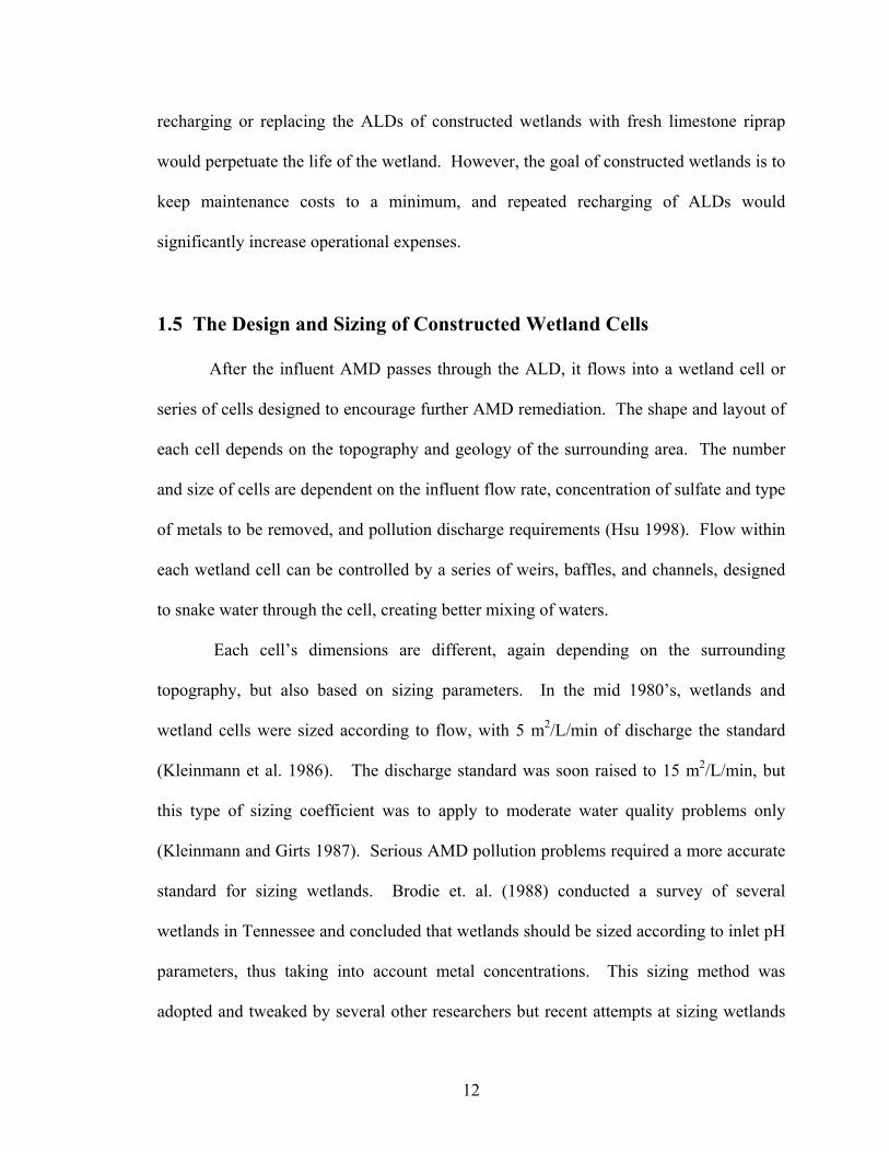
1.5 The Design and Sizing of Constructed Wetland Cells

After the influent AMD passes through the ALD, it flows into a wetland cell or

series of cells designed to encourage further AMD remediation. The shape and layout of

each cell depends on the topography and geology of the surrounding area. The number

and size of cells are dependent on the influent flow rate, concentration of sulfate and type

of metals to be removed, and pollution discharge requirements (Hsu 1998). Flow within

each wetland cell can be controlled by a series of weirs, baffles, and channels, designed

to snake water through the cell, creating better mixing of waters.

Each cell’s dimensions are different, again depending on the surrounding

topography, but also based on sizing parameters. In the mid 1980’s, wetlands and

wetland cells were sized according to flow, with 5 m2/L/min of discharge the standard

(Kleinmann et al. 1986). The discharge standard was soon raised to 15 m2/L/min, but

this type of sizing coefficient was to apply to moderate water quality problems only

(Kleinmann and Girts 1987). Serious AMD pollution problems required a more accurate

standard for sizing wetlands. Brodie et. al. (1988) conducted a survey of several

wetlands in Tennessee and concluded that wetlands should be sized according to inlet pH

parameters, thus taking into account metal concentrations. This sizing method was

adopted and tweaked by several other researchers but recent attempts at sizing wetlands

13

have taken a different, and more effective approach. In the recent approach, wetlands are

monitored for water quality and flow, and an average area-adjusted mass retention for

metals is determined (Eddy 1995). The average area-adjusted mass retention for metals

is then correlated with inlet pH and can be used as a guide for future wetland

construction. However, this approach is questionable from the standpoint that small

wetlands that receive higher metal loads and have a higher iron retention are not

necessarily the most efficient at metal retention over a large area. Thus, it has been

suggested by Eddy et al. (1995) that wetlands be sized using area-adjusted metal retention

data from wetlands producing water of a quality that exceeds federal and state standards.

Once an accurate sizing determination is estimated for a given mine drainage area,

construction of the wetland can begin.

1.6 Wetland Cell Substrate

Many organic substrates have been used in constructed wetlands. Cow manure

and mushroom compost seem to be the two most popular choices for substrate but

decomposed wood and sawdust have also proven effective at providing organic carbon to

the system (Gross et al. 1993). Crushed limestone is commonly used as a substrate to

increase alkalinity through the cell, as is the case at the Wills Creek Wetland in Ohio. In

the Midwestern wetland in Indiana, no substrate from offsite was used at all. Instead,

local material, including coal spoil was used to line the bottoms of cells.

14

1.7 Sulfate Reduction

Sulfate reduction has proven to be an effective means of raising pH and removing

metals and sulfate from AMD. Sulfate reducing bacteria use electron donors such as

SO42-, NO3-, and CO2, to oxidize simple organic compounds found in the substrate

(Singleton 1993). Hydrogen sulfide and bicarbonate ions are formed in the process.

Bicarbonate ions will consume protons in the system, elevating the pH of the system and

causing the precipitation of dissolved metal ions. The sulfate reduction process,

including oxidation of organic compounds and precipitation of metal sulfides can be seen

in the following equations:

2CH2O + SO42- 2HCO3

- + H2S

Me2+ + H2S MeS + 2H+

Sulfate reduction occurs due to the presence of sulfate reducing bacteria in the

wetland substrate coupled with sufficient organic material to stimulate their activity.

These bacteria are a group of prokaryotic microorganisms that use electron donors to

reduce sulfate (Hsu 1998). Evidence of sulfate reducers in wetlands include blackened

sediment due to the resulting precipitation of iron sulfides and the smell of hydrogen

sulfide (Fauque 1995). Dvork et al. (1992) suggested that six conditions should exist for

the sulfate reduction process to occur:

1) anaerobic conditions

2) a source of sulfate

15

3) a source or organic carbon

4) the presence of sulfate reducing bacteria

5) a way to physically retain metal sulfide precipitates

6) an influent pH of 5-6

The five wetlands studied have most of the six requirements. However, two of the five

wetlands have influent pH values lower than 5-6. Substrate for the wetland cells, such as

mushroom compost and cow manure, provide the source of organic carbon for the

system. Typha cattail roots provide a matrix for the physical retention of metal sulfides.

Typha cattails also provide an anaerobic environment, allowing sulfate reducing bacteria

to thrive. However, several of the wetlands studied have had their Typha plant

communities destroyed by muskrats or drowned by beavers. Also, the substrate for each

wetland varies from wetland to wetland and from cell to cell within a given wetland,

varying the amount of organic carbon provided for sulfate reducing bacteria.

The treatment of AMD by sulfate reduction is dependent upon a number of

independent factors. Thus, successful treatment may be affected by any minor change in

the status of one of the defining conditions above. However, if sulfate reduction operates

efficiently, constructed wetlands are a very effective alternative to wastewater treatment.

The effectiveness of sulfate reduction was studied in the five wetlands listed herein to

determine whether each wetland was performing up to initial wastewater treatment goals.

16

1.8 Use of Sulfur Isotopes to Determine the Efficiency of Sulfate Reduction

Sulfate reducing bacteria remove sulfate from the water column by metabolizing

sulfate into living tissue or by reducing sulfur to produce energy (Hsu 1998). Sulfur

isotopes, mainly 32S and 34S, are fractionated in the process and are represented by the

delta notation, δ34S. Harrison and Thode (1958), suggest that sulfur isotope fractionation

occurs in two main stages: 1) entrance of sulfate into the cell, brought primarily by AMD,

resulting in a small isotopic shift and 2) the breaking of S-O bonds, yielding a large

isotopic shift. Bacteria help break these S-O bonds, with 32S S-O bonds breaking much

easier than the heavier 34S isotope. Consequently, bacteria tend to fractionate 32S more

readily than 34S, resulting in an excretion of H2S enriched in 32S relative to original

sulfate. Thus, sulfur isotope ratios get progressively heavier in 34S in the water column

while the substrate gets enriched in 32S, the lighter isotope. Therefore, a sulfate reduction

trend should show sulfur isotope values going from a negative value to a less negative or

positive value. This trend should be seen in both water and soil samples. Soil samples

show this trend through the wetland because sulfate reducing bacteria have progressively

less 32S in the water column to fractionate. Thus substrate sulfide becomes progressively

heavier in 34S versus 32S

17

Chapter 2: History of Wetlands Studied Three constructed wetlands in Indiana and two in Ohio were studied to

determine their treatment efficiencies for sulfate and dissolved metal removal. Figure 2.1

and Figure 2.2 show the locations of the wetlands in each state.

Figure 2.1: Locations of Constructed Wetlands in Indiana

18

Figure 2.2: Locations of Constructed Wetlands in Ohio

19

2.1 Friar Tuck Wetland

The Friar Tuck volunteer wetland (Figure 2.3) is located in Southwest Indiana,

northeast of Dugger, Indiana, on the boundary between Sullivan and Greene Counties

(see Figure 2.1) (Comer 1997). Four coal beds were mined by surface and underground

methods and resulting spoil were mounded on top of the natural terrain or deposited in

low-lying slurry ponds (Branam and Harper 1994). The current remediation activity at

the site involves the Southeast Gob pile and acid mine drainage that enters the Mud

Creek surface drainage from this deposit. The Friar Tuck volunteer wetland was

proposed to test the applicability of a wetland treatment system for AMD abatement

(Comer 1997). The wetland itself is constructed around an old lake bed that is part of the

natural drainage pattern of the Friar Tuck site. Reconstruction of the lake to allow for its

use as a natural wetland involved damming of the north end of the lake to control effluent

flow to the Mud Creek and breaching of an acid pond that had formed due to drainage

from the Southeast Gob pile to allow flow into the newly redesigned wetland. The final

product is a cattail dominated lake with an inlet for acid mine drainage discharging from

a breached AMD pond (Smith 2000) and an inlet for fresh water to the southeast of the

AMD inlet. The AMD is brought from the breached pond to the wetland along a

limestone riprap channel where it mixes with the fresh water, then exits the wetland at the

northern end of the lake into the Mud Creek.

Effluent

InfluentFresh Water

InfluentAMD

FTS-3FTS-2A

FTS-1

250 feet

N<

Friar Tuck

< Flow

<<

<

Mu

d C

ree

k

Breached AMD Pond

FTS-2

Figure 2.3: Friar Tuck volunteer wetland showing sampling sites as well as influent and effluent locations

20

21

2.2 Tecumseh Wetland

The Tecumseh constructed wetland (Figure 2.4) located in Warrick County in

Southwest Indiana (Figure 2.1) has been operational for about 5 years and consists of five

cells through which acid mine drainage travels. The AMD discharges through an anoxic

limestone drain, an embankment designed to channel water through pore spaces of

limestone, increasing alkalinity and pH in the process. Cell 1 receives the initial

discharge into the wetland and channels this water into cell 2, which then discharges into

cell 3, then to cell 4. However, it is believed that the ALD is clogged and influent AMD

is being rerouted to cell 4A. Thus, cell 4A receives the bulk of the initial discharge of

AMD into the wetland. Fresh water enters cell 1, originally designed to provide an

alkalinity and pH boost to cell 1. This influent is now the major influent for cells 1, 2,

and 3 and eventually mixes with cell 4A effluent and flows into cell 5. Another fresh

water inlet flowing into cell 3 provides an additional boost to pH and alkalinity of cell 1

and 2 effluents in order to create a more desirable environment for the sulfate reducing

bacteria. The surface area of cell 5 is greater than the combined surface area of the other

four cells and serves mostly as a mixing and holding cell for effluents from the rest of the

wetland. Water exits the wetland at the southern end of cell 5. Flow into and through

each cell is controlled by berms, designed to create a snake-like flow that promotes better

mixing of waters. Vegetation is prolific throughout the wetland with the exception of cell

5, which seems to have been devastated by muskrats. Thus, minimal organic carbon is

being added to the system in cell 5, limiting the sulfate reduction process.

Effluent

Cell 5

Cell 4ACell 4

Cell 3

Cell 2

Cell 1

Anoxic Limestone

Lake

Drain

Fresh Water Supply

TCS 5 out

TCS 4 out

TCS 4A out

TCS 4 mid

TCS 4A inlet

TCS 4 inlet

TCS 3 2nd berm

TCS 3 fresh

TCS 2 out

TCS 1 out

Tecumseh

100 feet

N

<

<

Flow

<

<<

<

<<

<

<

<

<

<

<<

AMDInfluent

AMD Influent

TCS 1 fresh

Figure 2.4: Tecumseh Wetland showing sampling sites within each cell as well as influent, effluent and fresh water input sites

22

23

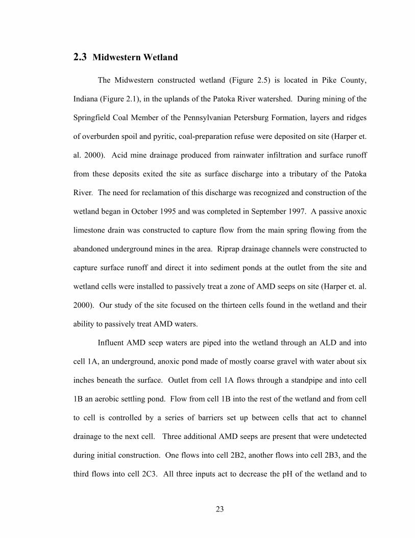
2.3 Midwestern Wetland

The Midwestern constructed wetland (Figure 2.5) is located in Pike County,

Indiana (Figure 2.1), in the uplands of the Patoka River watershed. During mining of the

Springfield Coal Member of the Pennsylvanian Petersburg Formation, layers and ridges

of overburden spoil and pyritic, coal-preparation refuse were deposited on site (Harper et.

al. 2000). Acid mine drainage produced from rainwater infiltration and surface runoff

from these deposits exited the site as surface discharge into a tributary of the Patoka

River. The need for reclamation of this discharge was recognized and construction of the

wetland began in October 1995 and was completed in September 1997. A passive anoxic

limestone drain was constructed to capture flow from the main spring flowing from the

abandoned underground mines in the area. Riprap drainage channels were constructed to

capture surface runoff and direct it into sediment ponds at the outlet from the site and

wetland cells were installed to passively treat a zone of AMD seeps on site (Harper et. al.

2000). Our study of the site focused on the thirteen cells found in the wetland and their

ability to passively treat AMD waters.

Influent AMD seep waters are piped into the wetland through an ALD and into

cell 1A, an underground, anoxic pond made of mostly coarse gravel with water about six

inches beneath the surface. Outlet from cell 1A flows through a standpipe and into cell

1B an aerobic settling pond. Flow from cell 1B into the rest of the wetland and from cell

to cell is controlled by a series of barriers set up between cells that act to channel

drainage to the next cell. Three additional AMD seeps are present that were undetected

during initial construction. One flows into cell 2B2, another flows into cell 2B3, and the

third flows into cell 2C3. All three inputs act to decrease the pH of the wetland and to

24

renew the concentrations of heavy metals in solution. Water exits the wetland at cell

2C7.

Effluent

InfluentAMD

2C7

2C6

2C5

2C4

2C3

2C2

2C1

2A

2B1

2B2

2B3

1B

1A

MWS 2C7

MWS 2C7 out

MWS 2C6 out

MWS2C6

MWS 2C5 out

MWS 2C5

MWS 2C4 out

MWS 2C4

MWS 2C3 out

MWS 2C3

MWS2C2out

MWS 2C2

MWS 2C1 out

MWS 2C1

MWS2B3 out

MWS 2B3 seep

MWS2B2 out

MWS2B2mid

MWS 2B2 seep

MWS 2Aout

MWS 2A

MWS 1Bout

MWS Standpipe

MWS 1Abott

MWS 1Atop

Midwestern

100 feetN

<Flow

<<

<

MWS 1B top

<

Freshwater Inlet

MWS 2B3

<

<

<

MWS 2C3 seep <

Figure 2.5: Midwestern wetland showing each cell, sampling sites, influent and effluent locations, and additional AMD seeps

25

26

2.4 Wills Creek Wetland

The Wills Creek wetland (Figure 2.6) was built in 1994 by the Division of

Reclamation of the Ohio Department of Natural Resources to remediate acid mine

drainage from underground coal mines in the Coschocton and Muskingum County areas

(Figure 2.2) (Hsu and Maynard 1999). The wetland drains into the Wills Creek

reservoir, a 22 mile-long lake that serves as the main tributary for the Muskingum River

(Hsu 1998). A 1987 study done by the Special Studies Section of the Abandoned Mined

Lands program determined that the source of acid mine drainage appearing in residential

drinking water wells originated from underground coal mines in the area. A follow up

study by Frank Brockmeyer (1987) of the Wills Creek reservoir showed that the

environmental effects of acid mine drainage from the underground coal mines were not

detrimental to the Wills Creek Lake itself, and were, in fact, minimized by the dilution of

the drainage by the large volume of water in the lake (Hsu 1998). The Wills Creek

wetland was thus built to lessen the environmental impact to drinking water wells of

several residences in the area (Brockmeyer 1987).

The wetland is divided into a series of small aeration pools, a settling pond, and

three cells through which AMD flows. Input to the wetland flows down a limestone

riprap channel and through an anoxic limestone drain which, at the time of sampling, was

believed to be clogged based on low input pH values. Aeration pools receive the ALD

treated water and promote iron oxide precipitation. AMD flows from the aeration pools

to the settling pond, a cell designed to allow precipitated metals from the aeration pools

to settle before entering the remaining cells (Hsu 1998). Next are cells 1 and 2 designed

to store metals and keep them immobilized. They are both vegetated with Typha latifolia

27

L. cattails throughout and were initially lined with varying types of compost materials.

Mushroom compost mixed with agricultural lime served as the substrate for cell 1 and a

50/50 mixture of mushroom compost and old cow manure mixed with agricultural lime

serves as substrate material for cell 2. Cell 3 is designed to receive subsurface flow from

cell 2, creating influent anaerobic conditions that encourage sulfate-reduction. The

substrate for cell 3 was a product called fermway, the trade name for fermented

chicken/cow manure (Hsu 1998). Effluent waters from cell 3 flow into the Wills Creek

reservoir.

100 feetN

SettlingPondCell 1

Cell 2Cell 3

Influent

Effluent

WC 1 bott WC 1topWC 2 top

WC 2 bottWC 3

Wills Creek

<

< Flow

overflow channel Overflow Channel seep

SettlingPond seep

Figure 2.6: Wills Creek wetland showing cell and sampling locations (Hsu and Maynard 1999, borrowed with permission)

28

29

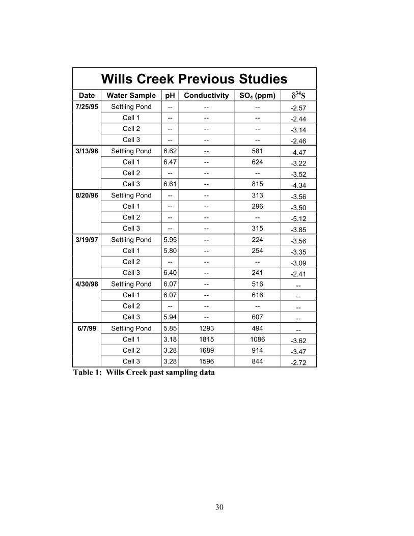
The Wills creek wetland was extensively sampled by Hsu and Maynard (1999)

and comparisons can be made between past and current data sets. Table 1 shows data

collected over a period of four years. Their conclusions suggest that the Wills Creek

wetland was not effective in removing sulfate based on a relatively consistent

concentration of SO4 through the system. Sulfate concentrations actually rise instead of

fall from the influent to effluent of the wetland for some of their data. Sulfur isotope data

also suggested that minimal sulfate reduction was occurring, with an average δ34S of –

3.36 and minimal change of the isotopic values from influent to effluent. The general

conclusion from the Hsu and Maynard work was that sulfate reduction was occurring at

Wills Creek but the effect was to small to have a significant remediation effect on AMD.

30

Wills Creek Previous Studies Date Water Sample pH Conductivity SO4 (ppm) δ34S

7/25/95 Settling Pond -- -- -- -2.57 Cell 1 -- -- -- -2.44 Cell 2 -- -- -- -3.14 Cell 3 -- -- -- -2.46

3/13/96 Settling Pond 6.62 -- 581 -4.47 Cell 1 6.47 -- 624 -3.22 Cell 2 -- -- -- -3.52 Cell 3 6.61 -- 815 -4.34

8/20/96 Settling Pond -- -- 313 -3.56 Cell 1 -- -- 296 -3.50 Cell 2 -- -- -- -5.12 Cell 3 -- -- 315 -3.85

3/19/97 Settling Pond 5.95 -- 224 -3.56 Cell 1 5.80 -- 254 -3.35 Cell 2 -- -- -- -3.09 Cell 3 6.40 -- 241 -2.41

4/30/98 Settling Pond 6.07 -- 516 -- Cell 1 6.07 -- 616 -- Cell 2 -- -- -- -- Cell 3 5.94 -- 607 --

6/7/99 Settling Pond 5.85 1293 494 -- Cell 1 3.18 1815 1086 -3.62 Cell 2 3.28 1689 914 -3.47 Cell 3 3.28 1596 844 -2.72

Table 1: Wills Creek past sampling data

31

2.5 Simco Wetland

Construction of the Simco wetland (Figure 2.7) near Coshocton, Ohio (Figure

2.2), was completed in November 1985 and was designed to treat acid mine drainage

discharging from underground mines (Stark et al. 1990). The initial design consisted of

three wetland cells in sequence separated by small settling pools (Stark et al. 1988) A

fourth wetland cell was added in 1989 for a total wetland system area of 4138 m2.

Influent flow configurations were changed in August 1987 (Stark et al. 1990), with one

half of the influent AMD flowing into cell 1 and the other half flowing along a side

channel into cell 2. The principal contaminant in the drainage is a high concentration of

iron. Inlet concentrations of iron at the time of construction averaged 125 mg/L while

recent inlet concentrations have averaged less than 100 mg/L. Removal of iron from the

influent waters has been successful since construction. Stark et al. (1994) stated that the

Simco wetland has retained about 75% of the iron received since it was built, with no

immediate signs of declining performance. It has been the most successful and the most

highly monitored wetland in the state of Ohio. Additional chemical treatment of effluent

waters was required during the early stages of operation, but the onsite chemical

treatment facility was removed in August 1993. Subsequent effluent water chemistry has

consistently met federal regulations.

Each cell was designed to be approximately 65 cm deep with an average water

depth of 11 cm. The cells were filled with a 15 cm thick layer of crushed limestone

followed by a 45 cm thick layer of spent mushroom compost substrate. Typha latifolia L.

cattails were planted to an initial density of 3-4/m2 but vegetative cover has grown to

include cattail-rice cutgrass (Leersia oryzoides) (Stark et al. 1990). Inlet waters pass

32

directly to cell 1 and to cell 2 via a small channel. Cell 1 and 2 outlet waters mix in a

settling pond and flow into cell 3, then to cell 4 and out of the system. Straw bales

situated throughout each wetland cell provide a source of organic carbon for the system

and slow the passage of water, increasing retention time. Weirs separate each cell and

each settling pond and channel the flow of water from cell to cell. Water exits cell 4

through a large, deep channel that carries water to three additional settling ponds. These

ponds were not considered in our study because they were not designed as remediation

ponds, but simply holding ponds for effluent water.

100 feet

Influent

Effluent

Cell 4

Cell 3

Cell 2

Cell 1Simco

< N

Sim 4 out

Sim 4 inlet

Sim 3 inlet

Sim 2 out

sim 2 inlet

Sim 1 out

Sim 1 inlet

<

Flow

<

< <

Old

Hig

hwal

l

<

<

<

<

Sim inlet

Sim 1 soil

Sim 2 soil

Sim 3 soil

Sim 4 soil

Figure 2.7: Simco wetland showing cells and sampling locations

33

34

Chapter 3: Analytical Methods 3.1 Introduction

Water and Soil samples were taken at the five constructed wetlands during the

winter and summer seasons. Seasonality of sampling was stressed to acquire data from a

dormant (late winter) and an active (late summer) season in order to compare each

wetlands performance during these periods. Water samples were taken at the influent and

effluent of each wetland as well as within each wetland cell and analyzed for dissolved

sulfate concentrations, metal concentrations, and sulfur isotope values. On-site

measurements of pH, Eh, Conductivity, and temperature were taken and approximately

250 mL of water from each sampling point was bottled and preserved in ice for transport

back to the lab. Soil grab samples were taken at a depth of around six inches within each

wetland cell and analyzed for sulfur isotopes, sediment mineralogy, total carbon, total

sulfur, and porewater sulfides. Soil samples were placed in plastic zip lock bags and

preserved in ice for transport to the lab.

3.2 Dissolved Sulfate Water samples were taken in the field using 250 ml bottles cleaned prior to the

sampling with alkanox soap and 3 flushes of distilled water. Samples were kept on ice in

the field and stored in a refrigerator in the lab. Samples were filtered using a 1.2 µm

Millipore filter to remove any suspended organic matter. Two tablets of NaOH were

added to the sample to drive the pH above 8 and to precipitate iron oxides. Precipitation

and subsequent filtration of the iron oxide insured a complete precipitation of sulfate and

35

prevented the formation of amorphous iron sulfate, which caused problems during

filtration. After iron oxide filtration, pH of the sample was lowered to below 4 using

nitric acid and Barium Sulfate (BaSO4) was precipitated by adding a barium chloride

solution of 100 g of BaCl2*2H2O to 1 liter of distilled water. A pH value of 4.0 or lower

insured that BaSO4 would precipitate instead of the undesired Barium Carbonate

(BaCO3). BaCO3 was found to cause inaccurate sulfur isotope readings when processed

through the mass spectrometer. The Barium Chloride solution was added to the water

sample until no further BaSO4 precipitation was noticed. Samples were then filtered

again using 1µm glass microfiber filters and the BaSO4 precipitate was washed

repeatedly with distilled water, then allowed to dry in a petrie dish at 70°C. The dried

samples were then weighed using a Mettler Toledo AB204 digital balance and ppm

sulfate values were calculated using the following: PPM (mg/l) SO4 = (mg BaSO4 *

411.5) / (250 ml) (Standard Methods 1971). Dried samples were weighed and loaded

into the mass spectrometer at Indiana University and analyzed for sulfur isotope δ34S

values.

3.3 Sulfides Native Sulfur, Acid Volatile Sulfur (AVS) and Chrome-Reducible Sulfur

Soil samples were taken for each site using a post-hole digger at an approximate depth

of six inches. Soil samples at the Simco wetland were taken at a depth of three and six

inches to acquire data on the change of composition with depth. Samples were kept on

ice in the field and stored in a freezer in the lab. Sulfur from each soil sample was

36

extracted according to a procedure originally established by Canfield (1986) as modified

by Bruchert (1995). Figure 3.1 below shows graphically the sulfur extraction process.

Figure 3.1: Flow chart of sulfur extraction procedures (Bruchert 1995)

37

Approximately 10 grams of soil was weighed into a dry, pre-weighed 19mm x 90 mm

cellulose extraction thimble using a digital balance and placed in a Soxhlet extraction

vessel. Copper shot was cleaned and added to a 250 ml flask and covered with 250 ml of

Methylene Chloride. The copper shot was cleaned in a separatory funnel using three

flushes of 6M HCl followed by three flushes of H2O to remove the acid, then three

flushes of methanol was used to remove the H2O followed finally by three flushes of

Methylene Chloride. The filled Erlenmeyer flask was then mated to the extraction vessel

and placed on a burner at mild heat for 8 hours. After cooling, the Methylene Chloride

was poured off into a 250 ml beaker to capture any residual organic material. The copper

shot was air dried and poured into a three-neck reaction vessel.

Extraction of the Native Sulfur, AVS Sulfur, and Chrome Reduced Sulfur was

done according to a two step procedure modified after Canfield et al. (1986). The Native

Sulfur phase was released as H2S from the copper shot in the three-neck reaction vessel

by the addition of 50 ml of 6N HCl under a sealed nitrogen atmosphere in the University

of Cincinnati’s sulfide extraction apparatus. AgNO3 was added to a 10ml test tube, which

was attached to the receiving end of the extraction apparatus. Heat and agitation were

added to the three-neck reaction vessel and the extraction process allowed to run for 8

hours. Reaction of the H2S with the AgNO3 test tube produced Ag2S, which was filtered

through a 1µm glass microfiber filter, washed with NH4OH to remove traces of of AgCl,

and then dried in a 50°C oven.

AVS sulfur was released as H2S by the addition of 50 ml of 6N HCl to

approximately 5 grams of post-Native Sulfur extraction soil in the extraction flask under

a sealed nitrogen atmosphere. Heat and agitation were added and the process allowed to

38

run for 3 hours. The released H2S was reacted with AgNO3, producing Ag2S, which was

again filtered through a 1µm glass microfiber filter, washed, dried in a 50°C oven, and

weighed. Remaining soil in the extraction flask was filtered using a 1µm glass

microfiber filter and the HCl solution poured off into a 250 ml beaker to be used for

soluble (AVS) sulfate precipitation. Chrome-reducible sulfur was extracted by flushing

the post AVS extraction soil back into the extraction flask using distilled water. 80 ml of

CrCl3 solution was added to the extraction flask, along with heat and agitation, and

allowed to run for 8 hours. Iron di-sulfides were subsequently reduced and converted

into H2S, which again reacted with the AgNO3 to produce Ag2S that was filtered using a

1µm glass microfiber filter, washed, dried in a 70°C oven, and weighed.

The percent sulfide in each soil sample was calculated as follows:

% S = [( Native Sulfur (g) * 32.07) / (32.07 + 2(107.87) ) /

Soil Sample Dry Weight (g)] * 100

3.4 Porewater Sulfides and Sulfates

Soil was sampled at a depth of six (6) inches and placed in ziplock bags on ice for

transport to the lab. Soil was spooned into plastic vials and placed in a Servall

Superspeed Centrifuge at the University of Cincinnati in order to separate water from the

soil. Porewater was then filtered using a Whatman 1.5 µm two-way filter into a 60 ml

bottle. Each 60 ml bottle contained approximately 2 ml of Zinc Acetate (ZnAc) solution.

Reaction between the filtered water and the ZnAc precipitated Zn2S. The Zn2S

precipitate was then captured on a 1 µm glass microfiber filter and dried in a 50°C oven.

39

Dried samples were then weighed and analyzed for sulfur isotope values in the mass

spectrometer.

Remaining porewater was then acidified and a solution of Barium Chloride was

added to precipitate Barium Sulfate. The samples were acidified to ensure that no

Barium Carbonate would precipitate. BaCl was added until no further BaSO4

precipitation occurred. BaSO4 precipitate was filtered using a 1 µm glass microfiber filter

and allowed to dry in a 50°C oven. Dried samples were then weighed and analyzed for

sulfur isotope values in the mass spectrometer.

3.5 Sulfur Isotopes There are four sulfur isotope species that exist in nature 32S, 33S, 34S, and 36S.

The two most abundant isotopes are 32S making up 95.02% of the species and 34S,

making up 4.21% of the species. The isotopic fractionation, δ34S, of the two species was

determined for each soil and water sample from each wetland. δ34S is calculated using

the following equation: [(34S/32S)sample – (34S/32S)standard] / (34S/32S)standard] *1000.

The standard used is Canyon Diablo Troilite (CDT), an iron meteorite that represents the

bulk earth sulfur isotopic composition (Faure 1986).

Precipitates of both water and soil samples from all five wetlands were analyzed

for their sulfur isotope ratios. Approximately 1.21 – 1.29 µg of BaSO4 precipitate and

~1.29 – 1.36 µg of Ag2S precipitate was weighed out on a microbalance balance at the

University of Indiana and mixed with ~1.25 µg of an oxidant, V2O5. The mixture was

placed into tin cups and analyzed by the Nuclide 6-60 mass spectrometer at Indiana

University for sulfur isotope determination.

40

3.6 %Carbon - %Sulfur The total % carbon and total % sulfur can be determined by analyzing powdered

soil samples on Indiana University’s LECO Carbon-Sulfur 224 analyzer. The machine

was calibrated with the LECO calibration standard “Carbon and Sulfur in White Iron”.

Post native sulfur extraction soils were dried and 250 mg of each were weighed out into

ceramic thimbles. Thimbles were then inserted into the LECO and fired until %C and

%S readings were complete.

3.7 Sediment Mineralogy In order to determine the alternate sinks for sulfate within each wetland cell, the

mineralogy of the soils were identified using the Siemans D500 X-ray diffractometer

machine at the University of Cincinnati. X-ray diffraction determines the d-spacing

between crystal lattices through the use of Bragg’s Law and produces diffraction peaks of

a specific amplitude and phase (Moore and Reynolds 1989). Each mineral possesses a

distinct peak and can be identified on the diffractogram printed out after the analysis.

Soil samples were powdered and pressed evenly into an aluminum powder holder,

inserted into the diffractometer, and analyzed from 2° to 50° two-theta, with a 0.05 step

for each second. The diffractograms were analyzed by identifying the strongest peak of a

given mineral and then searching for smaller peaks of that mineral.

3.8 Bulk Chemistry

Bulk chemistry of the soil samples was determined by using X-ray fluorescence

using the University of Cincinnati Rigaku 3070 spectrometer. Soil samples were

41

powdered using a tungsten carbide ball mill and then pressed into thin pellets using a

Spex 3624B X-Press 20-ton press. Samples were analyzed for U, Pb, Zn, Cu, Ni, Cr, V,

and Ba for ppm and %Fe2O3, %MnO and %TiO2. %Fe2O3 and %MnO were analyzed to

determine the quantity of precipitated metals in the soil samples. Concentrations were

calculated by regression using data from USGS rock and soil standards.

3.9 PHREEQC

Water sample field and laboratory concentration data were used to estimate the

saturation index (SI) of gypsum. Concentrations of Ca, Mg, Na, K, Fe, Mn, Cl, SO4, and

HCO3 as well as pH and temperature were input into PHREEQC, a geochemical

equilibrium program. PHREEQC can calculate speciation and saturation-indicies,

reaction-path reactions, mixing of solutions, and inverse geochemical modeling

(Parkhurst 1995). Results of the analysis for and SI value for gypsum can be found in

Appendix E. Minerals such as gypsum will precipitate in a system if SI is greater than

zero. Such a mineral is said to be super-saturated. If the SI value is slightly less than

zero, then the mineral is very close to saturation and may precipitate or dissolve. If the SI

value is significantly lower than zero, then no precipitation of the mineral will take place

and the mineral is said to be under-saturated.

42

Chapter 4: Results and Interpretation

4.1 Friar Tuck Results and Interpretation

4.1.1 Introduction

The Friar Tuck volunteer wetland in Southwest Indiana consists of a single, cattail

dominated lake with an inlet for acid mine drainage (AMD) and an inlet for fresh water

(Figure 2.3). The goal of the fresh water inlet is to provide a source of alkalinity and

high pH to boost the pH of the acid mine drainage and promote ideal conditions for

sulfate reducing bacteria. The mine drainage is brought to the lake from a constructed

AMD spring in the west along a limestone riprap channel where it mixes with fresh water

supplied by the main fresh water inlet located to the southeast. Water sample locations

for the AMD and fresh water inlets are designated FTS-2 and FTS-1 respectively. The

pH of the AMD inlet was much lower than the ideal pH for sulfate reducing conditions.

Thus, a water sample, FTS-2A, was taken near the center of the lake where mixing of the

two influent waters would likely take place and yield the best possible conditions for

sulfate reduction. A pH of 5.70 was measured in these mixed waters, an adequate level

for bacteria to thrive. An effluent water sample, FTS-3, was also taken at the northern

end of the lake to determine overall wetland performance. Soil samples were taken at

two locations, FTS-2 and FTS-2A, to compare an ideal sulfate reduction environment

with a non-ideal locale. Field and laboratory data for all samples are shown in Table 2

and a simplified flowchart containing all data can be found in Figure 4.1.

43

4.1.2 Soil Samples

Soil samples were analyzed for sulfur isotope values. Samples taken at FTS-2 and

FTS-2A show a significant increase in δ34S at FTS-2 (-18.75) compared to FTS-2A

(-29.60), 6 permil heavier than FTS-2A. Sulfate reducers in the soil, feeding on 32S,

create heavier δ34S values in the residual water column. As distance traveled through the

wetland increases, the sulfur isotopes in the substrate also get heavier in response to a

heavier sulfate in the water column. The opposite is seen here at Friar Tuck between the

two AMD influent points. Sulfur isotopes are getting lighter from the influent to the

effluent, suggesting sulfate reduction activity. However, black soil, a common sulfate

reduction product, was found around FTS-2A. Investigation radially from the sampling

location yielded very few dark soil samples, suggesting that if sulfate reduction is

present, it is highly localized around FTS-2A and occurs solely due to the mixing of

influent waters. Other locations throughout the lake with minimal mixing would likely

yield little sulfate reduction.

4.1.3 Water Samples

Water samples were analyzed for sulfate concentrations (ppm) and sulfur isotope

values and field measurements were taken for pH, Eh, Redox (mV), Conductivity, acidity

and alkalinity. Influent pH at the fresh water inlet was measured at 7.25 while influent

AMD pH was measured at 2.92. Resulting wetland effluent pH was 6.47, slightly lower

than the fresh water inlet but considerably higher than the AMD inlet, suggesting that

water chemistry has improved, probably due to dilution. Eh and Redox values show few

consistent trends. Acidity follows expected trends, with the highest concentration at the

44

AMD inlet. Effluent acidity concentrations were significantly lower, 34 mg/L, than inlet

AMD at 6220 mg/L. Alkalinity is the highest at the fresh water inlet at 173 mg/L but was

below detection at the AMD inlet. Alkalinity measured at the proposed mixing point,

FTS-2A, was 132 mg/L, slightly lower than the fresh water inlet, suggesting that mixing

is taking place between fresh water and AMD influents. Alkalinity at FTS-3 was

measured at 85 mg/L, lower than previous measurements and probably caused by

additional AMD seeps into the wetland.

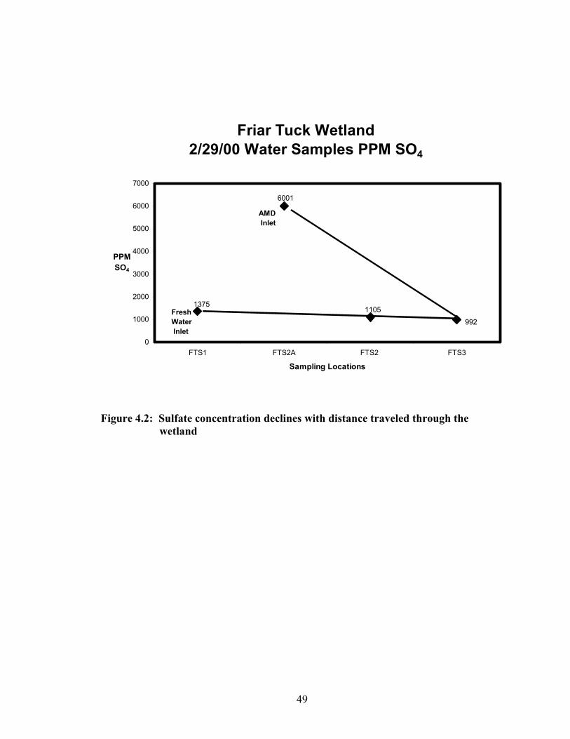
Sulfate concentrations from the water samples found in Table 2 show a decline

from the inlets of both AMD and fresh water, from 6001 ppm and 1375 ppm respectively

to an outlet concentration of 992 ppm. Figure 4.2 shows the decline of ppm SO4

graphically. The volume of influent freshwater is significantly greater than the volume of

influent AMD, suggesting that the small amount of AMD is being overwhelmed and

diluted by the freshwater input. Thus, an effluent concentration of 992 ppm is likely the

result of dilution and not sulfate reduction. However, the decline from 1375 ppm to 992

ppm suggests that some mechanism may be removing sulfate within the wetland,

possibly gypsum precipitation. Sulfur isotope values from water samples also do not

support sulfate reduction as a removal mechanism. Figure 4.3 shows that, δ34S, on

average, gets lighter as water travels through the wetland, exactly opposite of what would

be expected if sulfate reduction was occurring at Friar Tuck. The change of sulfur

isotopes to lighter values may be the result of additional, unknown fresh water inputs into

the wetland system. Fresh waters contribute isotopes with more 32S than 34S, thus making

resulting δ34S values more negative. Conductivity measurements in Table 2 support this

conclusion. These values can’t be balanced from influent to effluent without a significant

45

contribution of additional fresh water. Additional inputs of fresh water also supports the

extensive AMD dilution affect seen in sulfate concentration values. Thus, because

sulfate concentration and sulfur isotopes values don’t support conventional sulfate

reduction trends, I conclude that sulfate reduction is not a significant remediation process

at Friar Tuck wetland.

4.1.4 Conclusion

I believe the most active remediation process at Friar Tuck is dilution of influent

AMD. At the time of sampling, the volume of influent AMD was significantly less than

the volume of influent fresh water, based on conductivity values. Similarly, the volume

of effluent waters was significantly larger than the combined volume of both influents.

Also, effluent sulfate concentrations and conductivity values can’t be generated by

averaging both known influent concentrations and conductivities, suggesting other

sources of low conductivity/low sulfate concentration influents. Therefore, I believe that

multiple unknown freshwater inputs are actively contributing water to the system,

increasing alkalinity and pH and aiding in the dilution effect of the acid mine drainage.

Numerous drainage channels flowing into the wetland were noticed during sampling. It

is possible that periodic drainage of rainwater into the lake along these natural drainage

channels has a large but transitory affect on increasing alkalinity and pH. The mine

drainage contributes such a small volume to the lake that it is overwhelmed and diluted

by the input of fresh water.

It is to be noted that at the time of sampling, beavers had dammed the effluent

site, FTS-3, and caused the water in the lake to rise approximately 2 feet above normal

46

water elevation. Residence time of the water in the wetland was increased and cattails

were being drowned, reducing potential organic carbon input to the system. The longer

the residence time of the wetland, the longer sulfate reducing bacteria have to extract

sulfate from the water column, increasing the effectiveness of AMD remediation by

sulfate reduction. However, it is likely that the extra water volume in the lake would

have simply caused the suggested dilution process to become more apparent than it

would otherwise be under normal conditions.

47

Friar Tuck Wetland Field Measurements 2/29/00 Water

Samples pH Redox (mV) Eh Cond

(MS/cm) Acidity (mg/L)

Alkalinity (mg/L)

FTS-1 7.25 270 470 2.41 30 173 FTS-2 2.92 393 593 7.18 6220 0

FTS-2A 5.70 \ \ \ 32 132 FTS-3 6.47 347 547 1.597 34 85

Friar Tuck Water Samples

Friar Tuck Water Samples

2/29/00 δ34S

2/29/00 Dissolved

Sulfate (ppm)

FTS-1 2.89 1375 FTS-2 inlet 0.54 6001

FTS-2A -2.69 1105 FTS-3 0.76 992

Friar Tuck Soil Samples 2/29/00 Soil

Samples LECO

Sulfur % Native Sulfur

δ34S Native

Sulfur %

Chrome Reduced

Sulfur δ34S

Cr Reduced Sulfur %

FTS-2 0.3833 -18.75 0.0194 -22.54 0.1289 FTS-2A 0.0417 -29.60 0.0340 -29.95 0.2837

Table 2: Friar Tuck water and soil samples taken 2/29/00

>

>

>

Friar Tuck Wetland Sulfate and Sulfide Flow Chart

Sulfate 0.54

Sulfate 2.89

Sulfate -2.69

Sulfate 0.76

SulfideNatS -18.75 CrS -22.54

SulfideNatS -29.60 CrS -29.95

FTS 2A

FTS 1

FTS 2

FTS 3

Figure 4.1: Simplified flow chart showing sampling locations and accompanying laboratory data

48

49

Friar Tuck Wetland 2/29/00 Water Samples PPM SO4

6001

9921105

1375

0

1000

2000

3000

4000

5000

6000

7000

FTS1 FTS2A FTS2 FTS3

Sampling Locations

PPM SO4

AMD Inlet

FreshWater Inlet

Figure 4.2: Sulfate concentration declines with distance traveled through the

wetland

50

Friar Tuck Wetland 2/29/00 Water Samples δ34S

2.89

-2.69

0.76

0.54

R2 = 0.4753

-3

-2

-1

0

1

2

3

4

FTS 1 FTS 2 inlet FTS 2A FTS 3

Sample Locations

δ34S

Figure 4.3: Water sample δ34S values with distance traveled through the

wetland

51

4.2 Tecumseh Results and Interpretation 4.2.1 Introduction

The Tecumseh constructed wetland in Warrick County in Southwest Indiana

consists of 5 cells through which acid mine drainage travels (Figure 2.4). Acid Mine

Drainage is captured from various gob pile seeps by a large lake to the north of the

wetland. Water flows from the lake into cell 1 of the wetland through an anoxic

limestone drain built into a dam at the southern end of the lake. The ALD is designed to

increase the pH and alkalinity of the acidic lake waters. At present, the ALD is believed

to be clogged, and water has rerouted itself either beneath the dam and directly into cell

1, or around cell 1 and into the AMD inlet channel flowing into cell 4A. Due to the ALD

clogging, no significant increase in pH or alkalinity of lake waters is taking place. Input

to the wetland occurs at two other locations within the cells. Cell 1 and cell 3 receive

piped in fresh water intended to create a mixing of fresh water with acidic water and

encourage higher alkalinity and pH. Flow in each cell is controlled by berms, constructed

to create a snake-like flow pattern that promotes longer residence times and better

mixing. Water flows from the first four cells into cell 5 where a final mixing of all

surface water occurs. Cell 5 is significantly larger than the other four cells and serves as

more of a holding cell than as a remediation cell. Water exits the wetland to the south

along a limestone riprap channel.

Flow measurements were taken during the winter season between cells that had

adequate surface water flow and discharge rates and retention times for the wetland were

calculated. Results show that, on March 1st, 2000, Tecumseh had a discharge of 58,851

cm3/s. Residence time calculations suggest that the wetland had a retention time of 15.1

52

days. Rainfall data taken for the sampling period of March 1st, 2000 is shown

graphically in Figure 4.4 below and data taken for September 2000 is shown in Figure

4.5. Minimal rainfall occurred immediately before both sampling runs but the biggest

rainfalls before sampling occurred on February 18th and September 12th, both within the

calculated retention time for the wetland. Thus, a significant amount of recent

precipitation was in the system during both sampling dates, influencing field

measurements, discharge calculations, flow rates, and cell volume measurements.

Figure 4.4: February 2000 precipitation data shows minimal precipitation prior to

the March 1st sampling

53

Figure 4.5: September 2000 precipitation data shows minimal rainfall prior to the

September 19th sampling

4.2.2 Sampling

Tecumseh was sampled in the winter and summer seasons, March 1st, 2000 and

September 19th, 2000 respectively. Water and soil samples were taken at all probable

influent, mixing, and effluent points during winter 2000 and then at strategic points

throughout the wetland during summer 2000. Sampling locations are shown in the site

map (Figure 2.4). Field and laboratory data are shown in Table 3, Table 4, Table 5, and

Table 6. Influent water into cell 1 was measured at the western end of the cell as TCS-1

inlet fresh. Effluent from cell 1 to cell 2 was measured at sample location TCS-1 outlet at

the eastern end of cell 1, and input into cell 3 was measured at TCS-2 outlet near the

western end of cell 2. These two sample locations provide a convenient influent/effluent

comparison for cell 2. Cell 3 receives water from cell 2 as well as an additional fresh

water input. The fresh water supply was taken as sample TCS-3 inlet fresh. TCS-3 2nd

berm was taken at the second berm in cell 3 to determine whether there was mixing

54

taking place between the fresh water and the input from cell 2. Output from cell 3 occurs

at two locations. The larger volume of flow is into cell 5 through an overflow channel.

This outlet was not sampled due to inaccessibility and it is assumed that both outlets from

cell 3 have the same water chemistry because of their proximity. Remaining cell 3

effluent is channeled into cell 4 and the sample named TCS-3 outlet to cell 4.

Cell 4 is divided into cell 4 and cell 4A. Cell 4 receives its input solely from cell

3 while cell 4A receives its input solely from an acid mine drainage seep. I believe this

seep to be the main source of AMD flowing into the wetland. The effluent sample from

cell 4 is designated TCS-4 outlet. The influent seep sample into cell 4A is TCS-4A inlet

and the output from cell 4A to cell 5 is TCS-4A outlet. Also, a sample in the middle of

cell 4A was taken to determine any change in water chemistry as AMD travels through

the cell. March 1st, 2000 data suggests that pH actually decreases with distance traveled

through the cell. Further pH measurements at cell 4 and cell 4A outlets suggest that,

upon exit, the seep water hugs the southern berm of cell 4A without mixing with cell 4

and flows into cell 5. The division between the outputs from cell 4 and cell 4A is clearly

defined and pH measurements along a transect between samples. TCS-4A out and TCS-4

out reveal a sharp jump in pH values near the middle of the transect, suggesting that

waters are not mixing. Also, between the baffles separating cell 4A and cell 4 lies an

area that receives minimal water circulation of waters from either cell 4A or cell 4 and is

highly acidic due to this lack of mixing. Cell 5 receives both effluents from cell 4 and

cell 4A as well as cell 3 and serves as more of a lake than a wetland cell, with all three

inputs eventually mixing and exiting at the southern end of the cell at sample site TCS-5

outlet.

55

4.2.3 Water Samples

4.2.3.1 Field Measurements

Water samples were analyzed for sulfate concentration and sulfur isotope values

and field measurements were taken for pH, Eh, Redox (mV), Conductivity, acidity, and

alkalinity. Eh, Redox and Conductivity values change somewhat from input to output,

although change through the wetland is minimal. Influent and effluent pH values for

both sampling events are very similar. However, pH drops noticeably in cell 4A for both

seasons, with an inlet pH during winter 2000 of 4.6 and an outlet pH of 3.2. Eh, Redox,

and Conductivity also increase in this cell during the winter 2000 sampling but fall back

to levels characteristic of the rest of the wetland upon mixing with cell 4 and cell 3

effluents. Conductivity rises and pH falls during the summer. Acidity is highest at TCS-

4A outlet, as was expected due to the input of AMD to cell 4A. Acidity concentrations

fall to 18 mg/L at the effluent to the wetland, but influent concentrations were only 22

mg/L suggesting minimal influence from the AMD inlet on effluent wetland

concentrations. Alkalinity is relatively constant throughout the wetland, with the largest

concentration found, as expected, at cell 1, at 123 mg/L. Effluent alkalinity was 82 mg/L.

The overall change of field parameters for all sampling seasons is minimal, suggesting

that no significant remediation of AMD waters is occurring.

4.2.3.2 Sulfate Concentrations

Sulfate concentrations, measured in ppm SO4, from the winter and summer

seasons, shows little change with distance traveled through the wetland. Figure 4.6

shows the seasonal sulfate concentration trends. The influent concentration at cell 1 for

56

winter 2000 was measured at 1490 ppm while the effluent concentration was 1520 ppm.

However, significant amounts of SO4 were contributed to the system from the AMD

inlet, TCS-4A inlet, with a concentration of 2570 ppm. Effluent SO4 ppm from cell 4A,

5300 ppm, was significantly higher than the influent, at 2570 ppm. Thus, effluent waters

from cell 4A had significantly higher sulfate concentrations than influent waters,

suggesting that sulfate is entering the system from the substrate in cell 4A, not leaving the

system, as would be expected if sulfate reduction was occurring in cell 4A. Effluent

concentrations from cell 5 are significantly lower than the input to cell 5 from cell 4A.

Also, the volume of water leaving the system at TCS-5 outlet is much larger than the

volume exiting cell 4A. Therefore, I believe that the contribution of sulfate from the

outlet of cell 4A is overcome by the volume of low sulfate concentration waters from the

rest of the system and is diluted in cell 5. Thus, dilution seems to be the significant

remediation mechanism Tecumseh instead of sulfate reduction.

This conclusion is further supported by analyzing sulfate concentration trends

throughout the individual wetland cells. Influent SO4 concentrations increase by almost

300 ppm from cell 1 to the effluent from cell 2. Cell 2 represents a closed system, with

one input, and one output represented by TCS-1 out and TCS-2 out respectively. If

sulfate reduction was occurring in cell 2, sulfate concentrations would be falling, not

rising, as is the case during the winter season. Results from cell 3 show a similar

situation, with two inputs, TCS-2 out at 1760 ppm and TCS-3 inlet fresh at 1580 ppm.

When these two concentrations are averaged, the result is similar to what we have

measured for TCS-3 out, 1680 ppm. These findings indicate that, during the winter

season, sulfate concentrations are not being affected by sulfate reduction.

57

The summer season sampling shows similar sulfate concentration trends. Influent

fresh water into cell 1 was not measured but the resulting flow through cell 1 and cell 2

was captured at TCS-2 out, with a concentration of 1420 ppm. Resulting effluent from

the wetland at TCS-5 outlet was 1450 ppm, nearly identical to influent concentrations,

suggesting minimal if any overall change in sulfate concentrations throughout the

wetland. Lack of any decrease in sulfate concentrations during the summer suggests that

sulfate reduction is not a key player in the Tecumseh wetland system. The outlet from

cell 4A was significantly higher than other samples, with a concentration of 6530 ppm.

However, final effluent concentrations at TCS-5 outlet are significantly lower than the

output from cell 4A, suggesting that dilution seems to be the main player during the

summer. Combined volume from cells 1, 2, 3, and 4 amount to 41,767 m3 while the

volume of cell 4A is a mere 3,398 m3. The large volume of water from the other wetland

cells is overwhelming the small volume of AMD from cell 4A, causing dilution of the

drainage.

4.2.3.3 Sulfur Isotopes

Sulfur isotopes from water samples for both sampling seasons support the dilution

instead of sulfate reduction theory. Figure 4.7 shows the sulfur isotope values versus

distance traveled for both seasons. Both sampling event values are relatively scattered

but show no significant trend, suggesting little change in δ34S values. The isotope data,

shown in Table 4, is displayed in Figure 4.8 as a simplified flow chart of each wetland

cell. Data shows that the influent fresh water into cell 1 has a δ34S value of –3.57 while

the resulting effluent from cell 5 at TCS-5 outlet has a value of –3.46. This represents an

58

insignificant change from influent to effluent. Sulfate reduction, if occurring at

Tecumseh, would show a significant increase in 34S relative to 32S, resulting in a heavier

δ34S value. Also, individual wetland cells show minimal signs of sulfate reduction. For

example, effluent from cell 2 at TCS-2 out has a δ34S value of –3.61, almost identical to

the influent value at TCS-1 inlet fresh. No change in δ34S is occurring through these two

cells. Interestingly, the effluent δ34S value for TCS-3 out is identical to TCS-1 inlet at

fresh, -3.57. These values show no clear sulfate reduction trend through the first 3 cells

at Tecumseh.

Values for the second half of the wetland show similar trends, and isotope values

tend to get a lot lighter before getting any heavier. For example, effluent from cell 3 into

cell 4 has a δ34S value of –3.57 while effluent from cell 4 has a δ34S value of -6.64,

almost 3 permil lighter. Sulfate reduction would show the opposite effect, with isotope

values of the residual sulfate getting heavier, not lighter. Also, inlet AMD for cell 4A has

a δ34S value of –4.54 while the outlet value is 1.0 permil lighter, at –5.38. Clearly,

significant sulfate reduction is not occurring in cell 4A. TCS-5 outlet shows a heavier

δ34S value but this value is probably a product of dilution more so than sulfate reduction.

The dilution effect seen when comparing sulfate concentrations mimics the trends of the

isotopic values. The volume of water in cell 5 overwhelms the minimal AMD volume

from cell 4A, causing isotope values to increase. Similar isotope trends are seen in the

summer season. The δ34S value at TCS-2 outlet was –2.83 while the resulting effluent

value at TCS-5 outlet was -2.28, again very similar to the influent values and not a

significant sign of sulfate reduction.

59

4.2.3.4 Metal Concentrations

Water samples were taken at the influent and effluent of the wetland during the

winter 2000 season to determine the change in metal concentrations. Samples were

analyzed by Brookside Laboratory in New Knoxville Ohio. Only iron concentrations

were analyzed for this sampling run and the results can be found in Table 5. The data

suggests that iron concentration is falling, from an influent concentration of 1.5 ppm to an

effluent concentration below detection. Influent iron concentrations to the wetland

measured at the outlet from cell 1 are extremely low. Since the ALD at Tecumseh is

clogged, AMD is rerouting itself into cell 4A, bypassing cells 1 through 3. Perhaps a

water sample analyzed for metals at the influent to cell 4A would have shown a

significantly higher influent iron concentration and would better represent the input

parameters to the wetland. However, effluent concentrations were below detection

suggesting that Fe precipitation is occurring at Tecumseh. Thus, the influence of a large

volume of low Fe concentration freshwater may serve to dilute any measured iron

signature from the AMD inlet, resulting in a very low effluent concentration of iron at

cell 5 out.

4.2.4 Soil Samples

Soil samples were analyzed for Native Sulfur and Cr Reduced sulfur isotopes and

% sulfur. Samples were also analyzed for total percent sulfur using LECO combustion

and resulting values used to compare to Native Sulfur and Cr Reduced sulfur isotope

values. All values can be found in Table 6. No soil sample at TCS-5 outlet was taken

during either 2000 sampling season because the substrate consisted mainly of limestone

60

blocks and no significant quantity of soil could be found. Figure 4.9 shows how total %

sulfur relates to % Native Sulfur and Cr Reduced Sulfur for each soil sample. Minimal

correlation is present suggesting that the amount of Native and Cr Reduced sulfur in the

system is not directly related to total sulfur and that other sulfur species, including Acid

Volatile Sulfur, Pyrite sulfur, Bitumen sulfur, and Kerogen sulfur, are present in the

system. A more accurate correlation would be seen if these other species had been

analyzed.

Figure 4.10 shows winter 2000 native sulfur and chrome reduced sulfur δ34S

values with respect to distance traveled through the wetland. As sulfate reducing bacteria

extract 32S from the water column, they deposit sulfides enriched in 32S into the substrate.

As the water travels further through the wetland, its δ34S value gets heavier and the

resulting precipitating sulfides in the substrate also get heavier. Thus, if sulfate reduction

is occurring, δ34S values should get progressively heavier with distance traveled through

the wetland. The chrome reduced sulfur values show an overall trend of increasing δ34S

in the substrate. However, this trend is not seen in the native sulfur phase. Also, the

sulfate reduction trend of Cr Reduced sulfur is not supported by sulfate concentrations

nor by water sulfur isotope data. Therefore, we believe that the trend of increasing δ34S

values in the Cr sulfur phase is due to variations in substrate and the amount of organic

carbon present from cell to cell. The summer soil sample isotope data supports these

conclusions, but with only native sulfur data, no sulfur phase comparison could be made.

However, the change in δ34S values from TCS-2 out through the rest of the wetland is

minimal suggesting that sulfate reduction is not an active process in the summer. Water

61

data seems to be the easiest to understand and shows the most decipherable trends at

Tecumseh.

4.2.5 Conclusion

Dilution of influent AMD waters appears to be the primary remediation

mechanism at Tecumseh. Discharge from the wetland, 58,851 cm3/s, is overwhelmingly

large compared to the small volume of discharge of AMD into cell 4A of 1,270 cm3/s.

Sulfate concentration data support this conclusion based on the comparison of the high

concentration of SO4 from cell 4A to the low concentrations for both the input and the

output of the wetland. Sulfate concentrations tend to remain constant throughout the

wetland and only spike at the AMD inlet into cell 4A. The sole AMD contribution

appears to have minimal influence on the total sulfate in the system. Because sulfate

concentrations do not fall as water travels through the system, sulfate reduction is not the

main remediation mechanism in the wetland. Metal concentration data suggest that iron

is being removed from the system, but the extent of the data is limited. I believe that

simple dilution is the main player at Tecumseh, with the small influent AMD volume

being overwhelmed by the combined volume of fresh water from the rest of the wetland.

62

Tecumseh Wetland Field Measurements 3/1/00 Water


(MS/cm)

Acidity (mg/L)

Alkalinity (mg/L)

TCS-1 inlet fresh 6.82 @ 20.2C 80 280 4.22 \ \ TCS-1 outlet 6.57 @13.8C 228 428 2.64 22 123 TCS-2 outlet 6.83 @16.1C 228 428 2.64 24 84

TCS-3 inlet fresh 7.11 @15.1C 156 356 2.59 \ \ TCS-3 2nd berm 7.2 @14.4C 156 356 2.59 \ \

TCS-4A inlet 4.6@14C 279 479 4.73 \ \ TCS-4A outlet 3.18 @ 14.2C 373 573 4.37 1304 0 TCS-4A middle 3.42 @14.1C 370 570 3.99 \ \

TCS-4 inlet 6.53 @14.1C 216 416 2.61 \ \ TCS-4 outlet [email protected] 291 491 2.62 27 111 TCS-5 outlet 6.81 @17.9C 267 467 2.44 18 82

9/19/00 Water Samples pH Redox

(mV) Eh Cond (MS/cm)

Acidity (mg/L)

Alkalinity (mg/L)

TCS-1 inlet fresh 6.82 @ 20.3C -120 80 4.22 \ \ TCS-1 outlet \ \ \ \ \ \ TCS-2 outlet 6.45 @ 24.0 C \ \ 2.57 \ \

TCS-3 inlet fresh \ \ \ \ \ \ TCS-3 2nd berm \ \ \ \ \ \

TCS-4A inlet \ \ \ \ \ \ TCS-4A outlet 2.70 @ 27.8 C \ \ 8.13 \ \ TCS-4A middle \ \ \ \ \ \

TCS-4 inlet \ \ \ \ \ \ TCS-4 outlet 6.70 @ 26.6 C \ \ 2.79 \ \ TCS-5 outlet 6.07 @ 27.4 C \ \ 2.70 \ \

Table 3: Tecumseh water samples taken for winter and summer seasons

63

Tecumseh Water Samples Tecumseh

Water Samples 3/1/00 δ34S

3/1/00 Dissolved

Sulfate (ppm)

9/19/00 δ34S

9/19/00 Dissolved

Sulfate (ppm) TCS-1 inlet (Fresh) -3.57 1490 \ \

TCS-1 out -3.74 1650 \ \ TCS-2 out -3.61 1760 -2.83 1420

TCS-3 inlet fresh -3.27 1580 \ \ TCS-3 out -3.57 1680 \ \

TCS-4A inlet -4.54 2570 \ \ TCS-4A out -5.38 5300 -4.63 6530 TCS-4 inlet -3.58 1660 \ \ TCS-4 out -6.64 1640 -2.63 1610 TCS-5 out -3.46 1520 -2.28 1450

Table 4: Tecumseh water sample sulfur isotope and sulfate concentration data

Tecumseh Metal Concentrations Sample Date Fe (ppm) Mn (ppm) Ca (ppm) Na (ppm) K (ppm) Mg (ppm)

TCS-1 out 3/1/00 1.5 \ \ \ \ \ TCS-5 out 3/1/00 0 \ \ \ \ \ Table 5: Tecumseh influent and effluent metal concentrations

64

Tecumseh Soil Samples 3/1/00 Soil Samples

LECO Sulfur %

Native Sulfur δ34S

Native Sulfur %

Chrome Reduced Sulfur

δ34S Cr Reduced

Sulfur %

TCS-1 outlet 0.3213 -37.08 0.0253 -35.74 0.1010 TCS-2 outlet 1.472 -36.28 0.2623 -37.67 0.6242

TCS-3 2nd berm 0.4033 -26.18 0.0998 -31.23 6.3311 TCS-3 outlet 0.4926 -40.77 0.0191 -36.58 0.5104 TCS-4 outlet 0.5352 -8.46 0.0392 -16.11 0.0636 TCS-4A inlet 0.6733 \ 0.0018 -10.3 0.0255

TCS-4A middle 0.3765 -33.56 0.3468 -12.85 0.0548 TCS-4A outlet 0.2826 -32.78 0.2177 -14.68 \

9/19/00 Soil Samples

LECO Sulfur %

Native Sulfur δ34S

Native Sulfur %

Chrome Reduced Sulfur

δ34S Cr Reduced

Sulfur %

TCS-1 outlet \ \ \ \ \ TCS-2 out 0-5 1.024 -31.46 \ \ \

TCS-2 out 5-10 0.8456 -23.8 0.1980 \ \ TCS-3 outlet \ \ 0.0731 \ \

TCS-4 out 0-5 0.2374 -26.82 \ \ \ TCS-4 out 5-10 0.4264 -30.99 \ \ \ TCS-4A out 0-5 0.6504 -35.23 0.0074 \ \ TCS-4A out 5-10 \ -32.63 0.0083 \ \ Table 6: Tecumseh soil sample sulfur isotope and % sulfur data

65

Tecumseh Wetland SO4 Concentrations 3/1/00 vs 9/18/00

1680

2570

15201760 16401660

1490 1650 1580

5300

0

1000

2000

3000

4000

5000

6000

TCS 1inlet

(Fresh)

TCS 1 out TCS 2 out TCS 3inlet fresh

TCS 3 out TCS 4Ainlet

TCS 4Aout

TCS 4inlet

TCS 4 out TCS 5 out

Sample Location

PPM SO4

3/1/00

1420

6530

1610 1450

9/18/00

9/18/00

Figure 4.6: Winter and Summer 2000 sulfate concentrations trends with distance traveled through the wetland

66

Tecumseh Wetland 3/1/00 vs 9/18/00 Water Samples δ34S

-3.57

-5.38

-3.58

-6.64

-2.83

-3.61

-4.54

-3.46-3.57 -3.74

-3.27

-2.28-2.63

-4.63R2 = 0.201

-7

-6

-5

-4

-3

-2

-1

0

TCS 1inlet

(Fresh)

TCS 1 out TCS 2 out TCS 3inlet fresh

TCS 3 out TCS 4Ainlet

TCS 4Aout

TCS 4inlet

TCS 4 out TCS 5 out

Distance Traveled

δ34S

3/1/00 9/18/00

3/1/00

Figure 4.7: Water sample δ34S trends for winter and summer 2000

Tecumseh Wetland Sulfate Flow Chart

Cell 1

Cell 2

Cell 3

Cell 4A

Cell 3

Cell 4

Cell 5

>

>

>

>>

>>>

>

>>>

>FreshWaterSupply

FreshWaterSupply

AMD Inlet

AMD Inlet

>

3/1/00 -3.57

3/1/00-3.74

9/18/00-2.83

3/1/00-3.61

9/18/003/1/00-5.38 -4.63

3/1/00-4.54

3/1/00 9/18/00-6.64 -2.63

3/1/00 -3.27

3/1/00-3.57

>3/1/00-3.46

9/18/00-2.28

>

>

Figure 4.8: Flow chart of water sample sulfur isotope data from both sampling seasons

67

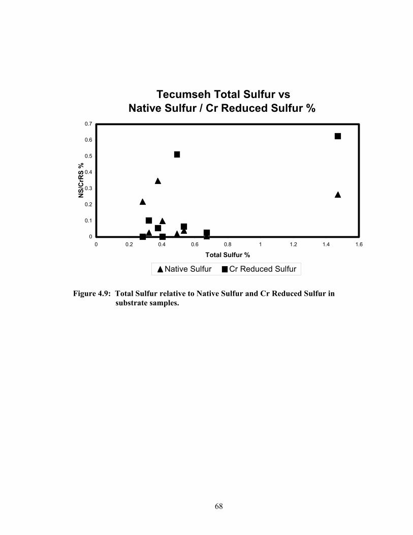
68

Tecumseh Total Sulfur vs Native Sulfur / Cr Reduced Sulfur %

0

0.1

0.2

0.3

0.4

0.5

0.6

0.7

0 0.2 0.4 0.6 0.8 1 1.2 1.4 1.6

Total Sulfur %

NS/

CrR

S %

Native Sulfur Cr Reduced Sulfur

Figure 4.9: Total Sulfur relative to Native Sulfur and Cr Reduced Sulfur in

substrate samples.

69

Tecumseh Wetland Native Sulfur / Cr Reduced Sulfur δ34S vs

Distance Travelled

-36.28

-26.18

-40.77

-8.46

-33.56-36.58

-16.11-12.85

-32.78-37.08

-14.68

-35.74

-37.67

-31.23

R2 = 0.761

-45

-40

-35

-30

-25

-20

-15

-10

-5

0

TCS-1 outlet TCS-2 outlet TCS-3 2ndberm

TCS-3 outlet TCS-4 outlet TCS-4A inlet TCS-4A middle

Sample Location

δ34S

Native Sulfur Cr Reduced Sulfur

Cr Reduced Sulfur

Figure 4.10: Native Sulfur and Cr Reduced Sulfur δ34S values with distance traveled

through the wetland

70

4.3 Midwestern Results and Interpretation

4.3.1 Introduction

The Midwestern constructed wetland consists of 13 cells through which acid mine

drainage travels (Figure 2.5). Acid mine drainage is channeled from numerous seeps on

site and is piped into the wetland through an anoxic limestone drain. Three additional

seeps, not discovered until after wetland construction was complete, enter cell 2B2 cell

2B3, and cell 2C3. Also, fresh water enters the wetland at cell 2A along a limestone

riprap channel. The channel is designed to capture precipitation runoff and channel it

into the wetland, providing a boost of high pH and high alkalinity. All influent waters are

channelized through the wetland and exit cell 2C7 in a riprap channel. Flow from cell 1A

is through a standpipe, which aerates the water and flows into cell 1B, an open air settling

pond. Flow between the remaining cells is controlled by a narrow channel 2 to 3 feet in

width. Cells are not internally baffled.

Flow measurements were taken during the winter months where any significant

flow was noticed between cells, and retention times and discharge rates were calculated.

Resulting calculations show that, on March 1st, 2000, Midwestern had a discharge of 840


days. Rainfall data taken before the sampling period of March 1st, 2000, is shown

graphically in Figure 4.11 and rainfall data taken before the September 18th, 2000

sampling is shown in Figure 4.12. Minimal rainfall occurred immediately before each

sampling run. However, since retention time for the wetland is 28.9 days, rainfall data

during the middle of February and the beginning of September suggest that a significant

71

amount of precipitation was in the system at the time of sampling, influencing field

measurements, discharge calculations, flow rates, and cell volume measurements.

Figure 4.11: February 2000 precipitation data shows minimal precipitation prior to

the March 1st sampling

Figure 4.12: September 2000 precipitation data shows minimal precipitation prior

to the September 18th sampling

72

4.3.2 Sampling

Midwestern was sampled in the winter and summer seasons of 2000, March 1st

and September 18th respectively and then again on February 23rd, 2001. Water samples

were taken at the influent and effluent of each cell and soil samples were taken near the

middle of each cell. Surface water and pore water samples were taken during winter

2001. A water sample was also taken at the two seeps entering cell 2B2 and cell 2B3 in

March 2000. All sampling locations are shown on the site map, Figure 2.5. Field data

are shown in Table 7 and 8 and laboratory data are shown in Tables 9, 10, and 11.

Influent water flowing into the ALD could not be sampled because flow is underground

but a water sample was taken at MWS-1A top, located in the gravel, polishing pond at the

beginning of the wetland. We have designated this sample as the influent AMD sample

for the system. Field measurements were taken at all water sample locations. The

measurements provide a glimpse of water quality throughout the wetland. No soil sample

was taken in cell 1A because the only substrate available was gravel. Effluent water

from cell 1A was taken at the standpipe between cell 1A and cell 1B and is designated

MWS-1A out. Effluent from cell 1B is designated. Effluent water samples were also

taken at the outlet of cell 2A and cell 2B1. The outlet from cell 2A captures any

freshwater contribution from the limestone riprap channel entering the cell. However, no

flow from the channel was entering the wetland at the time of sampling. The recently

discovered AMD seep into cell 2B2, MWS-2B2 seep, was sampled and the resulting

effluent from cell 2B2, MWS-2B2 out, was also sampled. MWS-2B2 represents the

combination of waters flowing through the wetland and the input of an additional seep.

MWS-2B3 out represents a similar combination, with effluent waters from cell MWS-

73

2B2 mixing with another AMD inlet, MWS-2B3 seep, and exiting into cell 2C1.

Subsequent water samples throughout the rest of the wetland, from cell 2C1 to 2C7, were

collected at the exit channels of every cell, thereby bracketing the influent and effluent

from each cell and allowing water quality changes from cell to cell to be observed. Soil

samples were taken at an approximate depth of 6 inches near the middle of each cell.

4.3.3 Water Samples


Water samples were analyzed for sulfate concentrations, metal concentrations,

and sulfur isotope values and field measurements were taken for pH, Redox (mV),

Conductivity, acidity, and alkalinity. All three sample seasons show a decrease in

conductivity with distance traveled through the wetland system. Also, all sample seasons

show a slight increase in pH from influent to effluent, with winter 2000 pH values of 6.53

at the influent and 7.34 at the effluent. The pH from water samples from winter 2000

falls at both AMD seeps, to 4.51 at MWS-2B2 seep and 3.60 at MWS-2B3 seep. All

three seasons show similar pH trends, with a winter 2000 influent pH of 6.53 and an

effluent pH of 7.34, a summer 2000 influent pH of 6.26 and an effluent pH of 7.09, and a

winter 2001 influent pH of 6.25 and an effluent pH of 6.71. The sulfate reduction

process functions well when initial influent pH is above 5-6 and remains high throughout

the wetland. Thus, pH measurements suggest that conditions are favorable for sulfate

reduction at Midwestern. Winter 2000 acidity and alkalinity data support this favorable

environment. Acidity is highest at cell 1A, the AMD input to the wetland, with a

concentration of 171 mg/L. Acidity falls through the wetland to an effluent concentration

74

of 15 mg/L. Thus, processes at Midwestern are effectively removing acidity from the

AMD. Alkalinity concentrations are significantly high in the cells near the beginning

wetland, with a cell 2A influent concentration of 188 mg/L. This high alkalinity provides

a boost for the system and promotes an ideal environment for sulfate reducing bacteria.


Sulfate concentrations, measured in ppm SO4, decrease almost 1000 ppm from the

influent to the effluent of the wetland during each of the three sampling seasons. Figure

4.13 shows the trends of sulfate concentrations with distance traveled through the

wetland for each season. Influent concentrations for the March 2000 sampling were 1740

ppm while the resulting effluent from cell MWS-2C7 was 831 ppm, a significant

decrease. Summer 2000 influent and effluent sulfate concentrations were measured at

2470 ppm and 1020 ppm respectively while influent and effluent sulfate concentrations

during the winter 2001 were 2118 ppm and 1282 ppm respectively. All three trends

represent significant decreases in sulfate concentrations with distance traveled through

the wetland. Sulfate reduction, when active in a wetland system, shows similar

reductions in sulfate with distance traveled, suggesting that sulfate reduction is a

potentially active process at Midwestern during each sampling season. However, sulfate

reduction cannot explain the fall in sulfate concentrations during the two winter sampling

seasons. The trend of sulfate concentration decline during the summer is much steeper

than either winter trend, suggesting an additional affect of sulfate reduction on the

removal of sulfate during the summer. The winter trends don’t show this additional

75

affect, suggesting other sulfate removal processes are occurring at Midwestern during the

winter seasons.

4.3.3.3 XRD Samples

Several sulfate removal processes are possible at Midwestern. One mechanism

for sulfate removal may be the precipitation of gypsum (CaSO4 + 2H2O) in the system.

Soil samples taken in each cell at Midwestern were ground into a fine powder and X-ray

peaks were measured using the University of Cincinnati’s Siemans D500 X-ray

diffractometer. Resulting data, found in Appendix E, show the presence of gypsum in

MWS-1B, MWS-2C2, MWS-2C5, and MWS-2C6. The other wetland cells show no X-

ray peak for gypsum. PHREEQC was used to determine the saturation index of gypsum

in these cells. Calculations suggest that gypsum is slightly under-saturated to slightly

super-saturated depending on the wetland cell. Thus, the presence of gypsum in some of

the cells at Midwestern suggests that the saturation index of gypsum fluctuates between

under-saturated and super-saturated conditions, possibly dependent on temperature.

Thus, sulfate removal by precipitation of gypsum does occur, but may not be

quantitatively significant based on the sporadic occurrence and apparent fluctuation of

saturation. It should be noted that the removal of sulfate alone is not a significant

remediation process because the process doesn’t remove any acidity from the water

column.

76


Sulfur δ34S values during summer 2000 are consistent with significant sulfate

reduction, but those from winter 2000 are not. Raw sulfur isotope data is shown in Table

8 and is also displayed in Figure 4.14 as a simplified flow chart of each wetland cell.

Figure 4.15 shows the change in isotopic values for the winter and summer 2000 seasons

and the winter 2001 season with distance traveled through the wetland. The trend for

March 2000 samples shows a relatively horizontal trend with distance traveled.

Corresponding wetland influent and effluent samples have a δ34S value of -5.31 and -5.56

respectively. Sulfate reduction should result in progressively heavier δ34S as distance

traveled through the wetland increases. However, the isotopic values don’t change

significantly, suggesting that bacterial sulfate reduction was not a significant remediation

process at Midwestern during the winter 2000 season. Winter 2001 samples show similar

trends, with an influent δ34S value of –4.88 and a corresponding effluent ratio of –4.31.

Therefore, I conclude that sulfate reduction is not a significant remediation process at

Midwestern during the winter seasons. Conditions are simply too cold for the sulfate

reducing bacteria.

Conditions during the summer appear to be more ideal for sulfate reduction. δ34S

values change from an influent value of –5.03 to an effluent value of +0.27 during

summer 2000. Sulfur isotopes get progressively heavier as distance traveled from source

increases. Figure 4.15 shows a clear increase in 34S and a resulting heavier δ34S value for

the summer season compared to the two winter season isotopic values. Thus, sulfate

reduction at Midwestern appears to be a significant remediation process during the

summer season.

77


Water samples were taken at the influent and effluent of the wetland to determine

the change in metal concentrations. Resulting data can be found in Table 10. Data shows

that iron (Fe) concentrations fall from an influent value of 101.73 ppm to 3.4 ppm at the

effluent, a significant decrease. Manganese (Mn) follows the same trend with an influent

concentration of 13.68 ppm and an effluent concentration of 5.39 ppm. Decrease in the

concentrations of these two metals indicates that significant metal precipitation is

occurring at Midwestern resulting in improved water quality. However, Federal Clean

Water Act regulations require 30-day discharges to be <3.5 mg/L for Fe and <2.0 mg/L

for Mn, significantly lower than measured values. Thus, while dissolved metal

precipitation is a significant process at Midwestern, further treatment of the effluent may

be required to meet water quality standards.

4.3.4 Soil Samples


% sulfur. All values can be found in Table 11. Figure 4.16 shows the trend of native

sulfur isotope values for samples from the winter 2000 season versus distance traveled

from source. The trend shows that sulfur isotopes get heavier as distance traveled

increases, suggesting that the sulfate reduction process is active in the winter. However,

sulfur isotope data from the water samples don’t support the trend of sulfate reduction

found in the substrate. The simple explanation is that a residual sulfate reduction trend is

being seen at Midwestern during the winter season. Sulfate reduction appears to be an

active process during the summer, based on summer 2000 water sample data. It is

78

possible that the sulfate reduction signature is frozen into the substrate during the winter

months and the resulting analysis of winter substrate samples suggests a sulfate reduction

trend that actually belongs to the summer season. However, while sulfur isotopes from

water sample data support sulfate reduction during the summer, isotopes from the

summer substrate samples don’t provide an accurate enough data set to suggest a trend of

sulfate reduction. Isotope values were simply too variable for an accurate interpretation

to be made. Water sample data is a much more reliable method of wetland interpretation.

Porewater samples were taken with corresponding surface water samples during

winter 2001 in the attempt to better understand substrate chemistry. Porewater sulfate

concentrations and δ34S values are shown in Table 9. Sulfate concentrations are variable

with distance traveled through the wetland and perhaps reflect the inherent variability of

the soil samples. Isotope values show a trend of decreasing δ34S with distance traveled

through the wetland, contrary to the expected trend of increasing δ34S seen in surface

water samples suggesting sulfate reduction. Note, however, that for 2A out and for 2C3,

porewater isotope values are significantly heavier than surface water values, consistent

with bacterial sulfate reduction. The last cell, 2C7, reverses this trend, suggesting that

sulfate reduction is not occurring in this cell.

4.3.5 Conclusion

Sulfate reduction is occurring at Midwestern, but mostly in the summer season

when conditions are ideal for bacteria to operate productively. Sulfur isotope trends for

water samples support this conclusion. Substrate samples from the summer are too

variable to allow for an accurate interpretation of substrate processes. However, it is

79

highly probable that sulfate reduction is an active process at Midwestern and that soil

samples are simply not the best way of detecting reduction trends. Sulfate reduction

during the winter season is not supported by sulfur isotopes from water samples but is

supported by substrate samples from that same season. I believe that the sulfate

reduction trend seen in the substrate samples from the winter season is simply a “frozen”

record of summer season activity at Midwestern. However, throughout all three seasons,

sulfate concentrations fall from the influent to the effluent of the wetland. This decrease

can be explained by sulfate reduction in the summer but another explanation is needed for

the winter seasons. The probable explanation is the precipitation of gypsum.

80

Midwestern Wetland Field Measurements 3/1/00 Water


(MS/cm)

Acidity (mg/L)

Alkalinity (mg/L)

MWS-1A top 6.53 @17C 9 209 3.69 171 0 MWS-1A bottom 7.25 @15.8C 28 228 \ \ \

MWS-1A out 6.74 @11.6C -24 176 2.83 122 0 MWS-1B out 7.19 @15.1C 252 452 2.52 \ \ MWS-2A out 7.21 @16.5C 233 433 2.26 35 188

MWS-2B2 seep 4.51 @12.4C 459 659 2.27 \ \ MWS-2B2 out 6.41 @ 13.1C 357 557 1.816 36 158

MWS-2B3 seep 3.60 @ 12.8 C \ \ \ \ \ MWS-2B3 out 5.48 @12.1C 418 618 1.771 40 17 MWS-2C1 out 5.82 @12.8C 414 614 1.801 \ \ MWS-2C2 out 6.31 @13.6C 396 596 1.779 26 42 MWS-2C3 out 6.65 @11.2C 378 578 1.632 \ \ MWS-2C4 out 6.90 @ 11.8C 377 577 1.517 \ \ MWS-2C5 out 7.22 @11.4C 356 556 1.488 \ \ MWS-2C6 out 7.29 @ 10.9C 355 555 1.34 \ \ MWS-2C7 out 7.34 @ 10.6C 355 555 1.34 15 76

9/18/00 Water Samples pH Redox

(mV) Eh Cond (MS/cm)

Acidity (mg/L)

Alkalinity (mg/L)

MWS-1A top 6.26 @ 17.4 C \ \ 3.64 MWS-1A bottom \ \ \ \

MWS-1A out \ \ \ \ MWS-Standpipe \ \ \ \

MWS-1B out 6.73 @ 21.0 C \ \ 3.02 MWS-2A out \ \ \ \

MWS-2B2 seep \ \ \ \ MWS-2B2 out 7.0 @ 14.1 C \ \ 2.25

MWS-2B3 seep \ \ \ \ MWS-2B3 out 7.11 @ 15.2 C \ \ 2.06 MWS-2C1 out 7.16 @ 15.7 C \ \ 2.07 MWS-2C2 out 7.20 @ 15.6 C \ \ 2.09 MWS-2C3 out 7.21 @ 15.4 C \ \ 1.95 MWS-2C4 out 6.99 @ 14.7 C \ \ 1.86 MWS-2C5 out 7.13 @ 13.8 C \ \ 1.9 MWS-2C6 out 7.13 @ 18.1 C \ \ 2.05 MWS-2C7 out 7.09 @ 15.3 C \ \ 1.87

Table 7: Midwestern water samples taken 3/1/00 and 9/18/00

81

Midwestern Wetland Field Measurements

Winter 2001 Water Samples pH Redox (mV) Eh Cond

(MS/cm) MWS-1A top 6.25 @ 9.4 C 11 211 2.82

MWS-1A bottom \ \ \ \ MWS-1A out \ \ \ \

MWS-Standpipe 6.09 @ 9.6 C 40 240 2.69 MWS-1B out 7.03 @ 9.4 C -11 189 2.63 MWS-2A out 6.03 @ 6.7 C 45 245 2.28

MWS-2B2 seep \ \ \ \ MWS-2B2 out 6.62 @ 6.1 C 53 253 1.97

MWS-2B3 seep 3.76 @ 5.5 C \ \ \ MWS-2B3 out 6.60 @ 5.4 C 81 281 1.74 MWS-2C1 out 6.41 @ 6.0 C 108 308 1.74 MWS-2C2 out 6.40 @ 5.2 C 119 319 1.66 MWS-2C3 out 6.42 @ 5.4 C 143 343 1.42 MWS-2C4 out 6.43 @ 4.8 C 147 347 1.43 MWS-2C5 out 6.67 @ 4.9 C 143 343 1.57 MWS-2C6 out 6.70 @ 5.5 C 142 342 1.54 MWS-2C7 out 6.71 @ 5.4 C 144 344 1.40

Table 8: Midwestern water samples taken 2/23/01

82

Midwestern Water Samples Midwestern Water

Samples 3/1/00 δ34S

3/1/00 Dissolved

Sulfate (ppm)

9/18/00 δ34S

9/18/00 Dissolved

Sulfate (ppm) MWS-1A top -5.31 1740 -5.03 2470 MWS-1A out -5.37 1600 \ \

MWS-1B standpipe -4.47 0 -4.79 2250 MWS-1B out \ 1540 -2.69 1980 MWS-2A out -4.26 1350 \ \

MWS-2B2 seep \ 1990 \ \ MWS-2B2 out -5.01 1230 -1.23 1540

MWS-2B3 seep -5.31 1440 \ \ MWS-2B3 out -4.66 1210 -0.98 1360 MWS-2C1 out -4.32 1230 -0.78 1370 MWS-2C2 out -4.66 1170 -0.46 1140 MWS-2C3 out -4.96 1050 -1.74 1370 MWS-2C4 out -5.35 903 -2.04 1300 MWS-2C5 out -5.79 932 0.34 1220 MWS-2C6 out -5.46 873 0.38 989 MWS-2C7 out -5.56 831 0.27 1020

Midwestern Water Samples

2/23/01 δ34S

2/23/01 Dissolved

Sulfate (ppm)

2/23/01 Pore Water

δ34S

2/23/01 Pore Water Sulfate

(ppm) MWS-1A top -4.88 0 / \ MWS-1A out / / / \

MWS-1B standpipe -4.73 2118 / \ MWS-1B out -3.87 2048 / \ MWS-2A out -4.22 1905 7.33 137

MWS-2B2 seep / / / \ MWS-2B2 out -4.40 1719 / \

MWS-2B3 seep / / / \ MWS-2B3 out -4.21 1715 / 48 MWS-2C1 out -3.78 1729 / \ MWS-2C2 out -4.05 1692 / \

MWS-2C3 seep -3.90 2212 / 214 MWS-2C3 out -5.50 1203 0.60 165 MWS-2C4 out -4.49 1381 / \ MWS-2C5 out -4.00 1582 / \ MWS-2C6 out -4.36 1458 / \ MWS-2C7 out -4.31 1282 -6.10 \

Table 9: Midwestern water sample sulfur isotope and sulfate concentration data

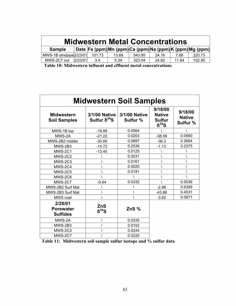
83

Midwestern Metal Concentrations Sample Date Fe (ppm) Mn (ppm) Ca (ppm) Na (ppm) K (ppm) Mg (ppm)

MWS-1B stndpipe 2/23/01 101.73 13.68 543.95 24.16 7.68 220.73 MWS-2C7 out 2/23/01 3.4 5.39 323.04 24.82 11.84 102.90

Table 10: Midwestern influent and effluent metal concentrations

Midwestern Soil Samples Midwestern

Soil Samples 3/1/00 Native Sulfur δ34S

3/1/00 Native Sulfur %

9/18/00 Native Sulfur δ34S

9/18/00 Native

Sulfur % MWS-1B top -19.89 0.0564 \ \

MWS-2A -21.22 0.0203 -38.58 0.0560 MWS-2B2 middle -30.66 0.0897 -36.3 0.2664

MWS-2B3 -14.72 0.2536 -1.13 0.2375 MWS-2C1 -13.45 0.0125 \ \ MWS-2C2 \ 0.0031 \ \ MWS-2C3 \ 0.0161 \ \ MWS-2C4 \ 0.0020 \ \ MWS-2C5 \ 0.0181 \ \ MWS-2C6 \ \ \ \ MWS-2C7 -0.64 0.0332 \ 0.0036

MWS-2B2 Surf Mat \ \ -2.96 0.6399 MWS-2B3 Surf Mat \ \ -43.86 0.4531

MWS coal \ \ -3.82 0.0871 2/28/01

Porewater Sulfides

ZnS δ34S ZnS %

MWS-2A / 0.0335 MWS-2B3 / 0.0152 MWS-2C3 / 0.0244 MWS-2C7 / 0.0225

Table 11: Midwestern soil sample sulfur isotope and % sulfur data

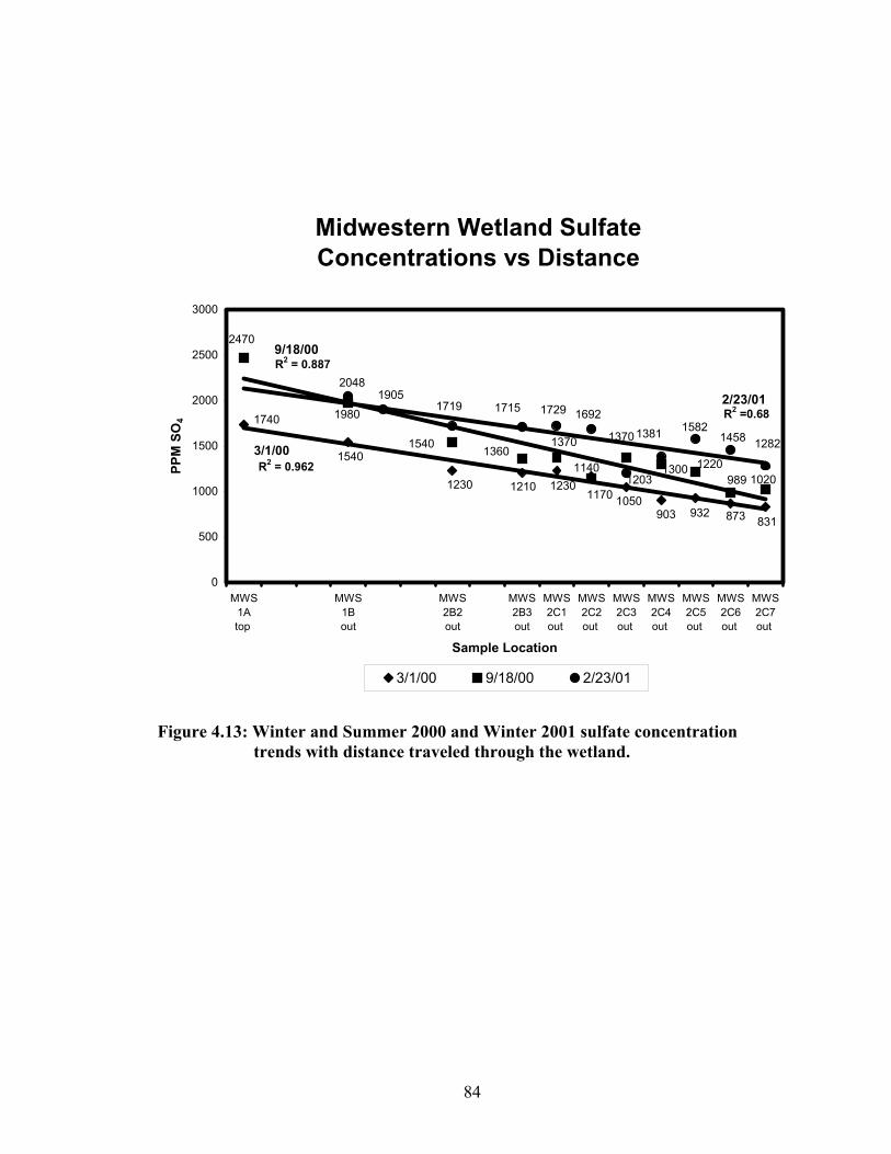
84

Midwestern Wetland Sulfate Concentrations vs Distance

8318739329031050

1210 12301170

1230

1540

1740

1020

2470

1140

1980

13601540 1370 1370

1300 1220989

1905

1282145815821381

1203

1692172917151719

2048

R2 = 0.962

R2 = 0.887

R2 =0.68

0

500

1000

1500

2000

2500

3000

MWS1Atop

MWS1Bout

MWS2B2out

MWS2B3out

MWS2C1out

MWS2C2out

MWS2C3out

MWS2C4out

MWS2C5out

MWS2C6out

MWS2C7out

Sample Location

PPM

SO

4

3/1/00 9/18/00 2/23/01

3/1/00

9/18/00

2/23/01

Figure 4.13: Winter and Summer 2000 and Winter 2001 sulfate concentration

trends with distance traveled through the wetland.

Midwestern Wetland Sulfate Flow Chart

1A

1B

2A

2B1

2B2

2B3

2C1

2C1

2C2

2C3

2C4

2C5

2C6

2C7

>>

>>

>

>>

>>

>

> >

>

>

>

>

AMD Inlet

AMD Inlet

AMD Inlet

3/1/00 -5.37

3/1/00 -5.31

MWS 1B standpipe 3/1/00 -4.47

3/1/00 -4.26

3/1/00 -5.01

3/1/00 -5.31

3/1/00 -4.66

3/1/00 -4.32

3/1/00 -4.66

3/1/00 -4.96

3/1/00 -5.35

3/1/00 -5.79

3/1/00 -5.46

3/1/00 -5.56

9/18/00 -2.69

9/18/00 -4.79

9/18/00 -1.23

9/18/00 -0.98

9/18/00 -0.27

9/18/00 0.38

9/18/00 0.34

9/18/00 -2.04

9/18/00 -1.74

9/18/00 -0.46

9/18/00 -0.78

9/18/00 -5.03

>

>

2/23/01 -4.88

2/23/01 -4.73

2/23/01 -3.87

2/23/01 -3.78

2/23/01 -4.05

2/23/01 -5.50

2/23/01 -4.49

2/23/01 -4.00

2/23/01 -4.36

2/23/01 -4.31

2/23/01 -4.88

2/23/01 -4.40

2/23/01 -4.21

AMD Inlet

>

2/23/01 -3.90

2/23/01 -4.22

3/1/00 -4.26

Figure 4.14: Flow chart of water sample sulfur isotope data from all three sampling seasons

85

86

Midwestern Wetland Water Samples δ34S

-4.66-4.96

-5.56

-1.74-2.04

-5.31-5.35

-4.32-4.66

-4.47

-5.46-5.79

-5.01

0.27

-5.03

-1.23

-0.46-0.78-0.98

0.380.34

-4.79

-5.5

-4.49

-4.05-3.78

-4.88-4.73

-4.4-4.21 -4.31

-4.36-4

R2 = 0.211

R2 = 0.773

R2 = 0.086

-7

-6

-5

-4

-3

-2

-1

0

1

MWS 1A to

p

MWS 1B st

andp

ipe

MWS 2B2 o

ut

MWS 2B3 o

ut

MWS 2C1 o

ut

MWS 2C2 o

ut

MWS 2C3 o

ut

MWS 2C4 o

ut

MWS 2C5 o

ut

MWS 2C6 o

ut

MWS 2C7 o

ut

Sample Locations

δ34S

3/1/00 9/18/00 2/23/01

3/1/00

9/18/00

2/23/01

Figure 4.15: Change in water sample isotopic values for winter and summer

2000 and winter 2001 with distance traveled through the wetland

87

Midwestern Wetland 3/1/00 vs 9/18/00 Soil Samples δ34S

-19.89

-30.66

-13.45

-0.64

-36.3

-14.72-21.22

-38.58

-1.13

R2 = 0.527

R2 = 0.796

-45

-35

-25

-15

-5

5

15

25

35

MWS-1B top MWS-2A MWS 2B2middle

MWS 2B3 MWS 2C1 MWS 2C7

Sample Locations

δ34S

3/1/00 9/18/00

3/1/00

9/18/00

Figure 4.16: Native sulfur isotope values for soil samples from 3/1/00 and 9/18/00

versus distance traveled through the wetland

88

4.4 Wills Creek Results and Interpretation

4.4.1 Introduction

The Wills Creek wetland in Zanesville, Ohio consists of 2 aeration ponds, a

settling pond, and 3 cells through which acid mine drainage travels (Figure 2.6). Acid

mine drainage from underground coal mines is channeled to the wetland along a

limestone riprap channel. Influent AMD passes through an anoxic limestone drain,

which serves to increase input pH and alkalinity. However, influent pH into cell 1 on

March 1st was 4.14, suggesting that the drain is clogged. After exiting the ALD, acid

mine drainage enters a series of stepped aeration pools lined with limestone and designed

to increase alkalinity and promote an aerobic environment, thus precipitating some heavy

metals before their passage into the wetland (Hsu 1998). Aeration pool effluents enter

the large, unvegetated settling pond, designed to allow precipitated metals from the

aeration pools an area to settle out of solution. Water then passes to cell 1, a vegetated

cell with a mushroom compost/agricultural lime substrate designed to further promote

dissolved metal precipitation. Water from cell 1 flows to cell 2 through a 5-foot wide

channel. Cell 2 is lined with a mushroom compost and agricultural lime substrate and is

heavily vegetated. Alternating in the upper portion of the cell are baffles designed to

regulate the flow of water through the beginning of the cell. Effluent from cell 2 flows

through a 10 inch PVC pipe underground into cell 3 (Hsu 1998). The substrate of cell 3

consists of crushed limestone topped with an organic substrate. Cell 3 is designed to

encourage sulfate reduction by providing subsurface flow and anaerobic conditions.

Water exits the wetland from cell 3 and flows into the Wills Creek reservoir system.

89


flow was noticed between cells and retention times and discharge rates were calculated.

Results show that, on March 9th, 2000, Wills Creek had a discharge of 1190 cm3/s.

Residence time calculations suggest that the wetland had a retention time of 7.34 days.

Previous residence times measured by Hsu 1998 were significantly lower at 2.42 days.

Differences in residence time measurements may be due to local conditions at the time of

sampling such as abnormal precipitation. Rainfall data taken March 2000 is shown

graphically in Figure 4.17 and rainfall data taken August 2000 is shown in Figure 4.18.

No rainfall occurred before the March 9th sampling suggesting that conditions at the time

of sampling reflect normal conditions and not conditions that might exist due to abnormal

precipitation. However, there was significant rainfall on the August 24th, 2000 sampling,

and several days before, suggesting that recent precipitation in the system may have

affected our field measurements, discharge calculations, flow rates, and cell volume

measurements for the August sampling.

Figure 4.17: March 2000 precipitation data shows no precipitation prior to the March 9th sampling

90

Figure 4.18: August 2000 precipitation data shows significant rainfall the day of sampling, affecting residence times and discharge calculations

4.4.2 Sampling

Wills Creek was sampled in the winter of 2000 and during the summer of 2000.

Water samples were taken at the influent and effluent of each cell and soil samples and

pore water samples were taken near the middle of each cell. Sampling locations are

shown on the site map (Figure 2.6). Field and laboratory data are shown in Tables 12

through 15. Influent AMD to the wetland was measured as WC-settling pond seep and is

located on the western end of the settling pond. Effluent water from the settling pond to

cell 1 was sampled as WC-1 inlet and subsequent effluent from cell 1 and cell 2 are

designated WC-1 out and WC-2 out respectively. These samples bracket each cell and

allow for the performance of each cell to be assessed. A water sample from cell 3 was

taken near the center of the cell and represents the effluent water chemistry of the system.

Soil samples were taken at the beginning and end of cell 1 and cell 2, providing a

91

comparison of beginning substrate composition with end composition. A soil sample was

also taken near the center of cell 3.

4.4.3 Water Samples



and sulfur isotope values and field measurements were taken for pH, Redox (mV) and

Conductivity. Influent water chemistry was very similar to effluent water chemistry in

2000. Influent pH was measured was measured at 4.14 on March 1st, 2000 while effluent

pH was 3.93. Notice that the pH actually decreases from influent to effluent, opposite of

the original treatment goal of the wetland. Redox and Conductivity values tend to remain

constant throughout the wetland as well, suggesting that little treatment of water is

occurring in the wetland.


Sulfate concentrations measured in ppm SO4, however, show decreases during all

three seasons of sampling. Figure 4.19 shows each season sulfate concentration trends

with respect to distance traveled through the wetland. Winter 2000 values show a

significant decrease, from 2540 ppm in the settling pond to an effluent concentration of

797 ppm. Summer 2000 data shows a decrease, but not nearly as drastic as that during

both winter seasons. During summer 2000, the settling pond influent sulfate

concentration was 1050 ppm while the effluent value was 975 ppm. While the change in

concentration from influent to effluent was not drastic, the initial input concentration was

92

significantly lower than both winter season inputs suggesting that sulfate production is

not as intense in the summer as it is during winter months. The decrease in sulfate

concentrations during both sampling seasons suggests that a sulfate removal process is

active at Wills Creek.


While sulfate concentrations suggest sulfate removal, sulfur isotopes do not

indicate bacterial sulfate reduction. Influent and effluent δ34S values remain relatively

constant throughout both seasons. Figure 4.20 shows the change of sulfur isotopes for

both seasons from the influent to the effluent. The raw data, shown in Table 13 is also

displayed in Figure 4.21 as a simplified wetland flow chart. Winter 2000 data shows an

influent δ34S value of –3.36 and a corresponding effluent value of –3.48. Summer 2000

values show a brief δ34S increase in cell 2 but resulting effluent from the system is –2.87

permil, only one permil heavier than the corresponding influent isotope value. The lack

of any trend towards heavier isotope values with distance traveled through the wetland

suggests that sulfate reduction is not a significant remediation process at Wills Creek

during either season. However, sulfate concentrations still fall during both seasons,

suggesting that sulfate removal is being caused by another process. Several sulfate

removal processes are possible at Wills Creek. One sink for sulfate may be the

precipitation of gypsum in the system. Soil samples taken by Hsu and Maynard (1999),

were analyzed using the University of Cincinnati’s X-ray Diffractometer and show that

gypsum was abundant. PHREEQC modeling of water chemistry showed that the surface

waters were at or very near saturation in cells 1 and 2 and in the settling pond. Gypsum

93

crystallization pulls sulfate from the water column and is likely to be the cause of the

sulfate concentration decrease seen at Wills Creek.


Water samples were taken at the influent and effluent of the wetland for the

winter and summer 2000 sampling seasons to determine the change in metal

concentrations. Resulting data can be found in Table 14. Data shows that during winter

2000, Fe concentrations fell from 12.6 ppm at the influent to 4.2 ppm at the effluent.

Summer 2000 showed a similar decrease in concentrations, from 10.10 ppm to 4.30 ppm.

Both trends suggest that iron precipitation is occurring at Wills Creek during both

seasons. Manganese concentrations for both seasons stay relatively constant, with

influent and effluent concentrations for winter 2000 of 8.45 ppm and 7.91 ppm

respectively. Summer 2000 concentrations actually rise slightly, from 6.72 ppm at the

influent to 6.90 at the effluent. Thus, while iron removal is occurring, manganese

concentrations are not affected. Federal Clean Water Act regulations require 30-day

discharges to be <3.5 mg/L for Fe and <2.0 mg/L for Mn, significantly lower than

measured Fe or Mn discharge concentrations. Thus, further treatment of the effluent to

help remove more iron and manganese may be required to meet water quality standards.

4.4.4 Soil Samples

Soil samples were analyzed for Native and Cr Reduced sulfur isotopes and for

% sulfur. All values can be found in Table 15. Figure 4.22 is a plot of sulfur isotope

values versus distance traveled for Native sulfur and Cr Reduced sulfur samples from the

94

winter 2000 season and shows Native sulfur isotope values from the summer 2000

season. The values are highly variable from sample to sample and no specific trend can

be determined. However, values from the influent to the effluent of each wetland cell

remain relatively constant throughout with the exception of the change in cell 1 during

the winter 2000 sampling. The influent substrate sample for cell 1 has a native sulfur

isotopic value of –31.7 and a Cr sulfur isotope value of –31.11 while the effluent sample

from cell 1 has a significantly heavier native sulfur isotope value of –6.1 and a

corresponding Cr sulfur isotope value of –6.61. Such a drastic changes in δ34S values

could suggest that sulfate reduction is a significant remediation process in cell 1 at Wills

Creek. However, this change is not seen through any of the other cells and is not

supported by the influent/effluent water sample isotope data. The drastic change in cell 1

could simply be another good example of the large degree of variability present when

analyzing sulfur isotopes from substrate samples.

4.4.5 Conclusion

Sulfate reduction is not a significant process in AMD remediation at the Wills

Creek wetland. The fall of sulfate concentrations for both seasons suggest sulfate

removal, but sulfur isotopes for water samples suggests the removal process is not sulfate

reduction. Gypsum precipitation is the likely process. Sulfur isotopes from water

samples for both sampling seasons don’t show a sulfate reduction trend and sulfur

isotopes from soil samples are too variable to allow for an accurate interpretation of

sulfate reduction from substrate samples. Also, based on influent pH measurements, the

95

ALD is clogged, preventing the system from receiving influent water quality sufficient

for sulfate reduction to occur.

Wills Creek Wetland Field Measurements

3/1/00 Water Samples pH Redox (mV) Eh Cond

(MS/cm) WC-settling pond seep 6.52 @ 12.7C 118 318 1.503

WC-settling pond \ \ \ \ WC-1 inlet 4.14 @ 17.1C 407 607 1.985 WC-1 out 4.04 @ 10.3C 450 650 1.741 WC-2 out 4.10 @ 12.8C 452 652 1.052 WC-3 out 3.93@ 13.1C 435 635 1.557

WC-outside channel seep 6.42 127 327 1.439 8/24/00

Water Samples pH Redox (mV) Eh Cond (MS/cm)

WC-settling pond seep \ \ \ \ WC-settling pond \ \ \ \

WC-1 inlet 3.40 @ 23.4 C \ \ 1.49 WC-1 out \ \ \ \ WC-2 out 3.61 @ 21.6 C \ \ 1.17 WC-3 out 3.48 @ 22.5 C \ \ 1.38

WC-outside channel seep \ \ \ \ Table 12: Wills Creek water samples taken 3/1/00 and 8/24/00.

Wills Creek Water Samples Wills Creek Water


3/9/00 Dissolved

Sulfate (ppm)

8/24/00 δ34S

8/24/00 Dissolved

Sulfate (ppm)

WC-Settling Pond Seep -4.31 656 \ \ WC-Settling Pond \ 2540 \ \

WC-1 inlet -3.36 \ -3.96 1050 WC-1 out -3.39 1200 \ \ WC-2 out -3.32 570 -1.67 1060 WC-3 out -3.48 797 -2.87 975

WC-Outside Channel Seep -4.31 631 \ \ Table 13: Wills Creek water sample sulfur isotope and sulfate concentration data

96

Wills Creek Metal Concentrations Sample Date Fe (ppm) Mn (ppm) Ca (ppm) Na (ppm) K (ppm) Mg (ppm)

WC-1 inlet 5/11/00 12.6 8.45 949 27.6 6.0 49.9 WC-3 out 5/11/00 4.2 7.91 996 27.6 7.4 49.4 WC-1 inlet 8/24/00 10.10 6.72 983 35.9 6.5 46.2 WC-3 out 8/24/00 4.30 6.90 1068 28.2 10.0 44.7

Table 14: Wills Creek influent and effluent metal concentrations

Wills Creek Soil Samples 3/9/00

Soil Samples Native Sulfur δ34S

Native Sulfur %

Chrome Reduced

Sulfur δ34S

Cr Reduced Sulfur %

WC-1 top -31.7 0.0282 -31.11 1.5716 WC-1 bottom -6.1 0.4415 -6.61 0.2773

WC-2 top ??? 0.1370 -17.14 0.3162 WC-2 bottom -27.63 0.1200 -36.06 0.1023

WC-3 -41.77 0.2806 -28.94 0.7463


Native Sulfur δ34S

Native Sulfur %

Chrome Reduced

Sulfur δ34S

Cr Reduced Sulfur %

WC-1 -24.31 0.1178 \ \ WC-2 -31.66 0.0720 \ \ WC-3 -36.04 0.0575 \ \

WC Coal -0.36 0.0699 \ \ WC Cattail \ 0.0009 \ \

Table 15: Wills Creek soil sample sulfur isotope and % sulfur data

97

Figure 4.19: Sulfate concentrations trends with distance traveled through the

wetland

W ills Creek W etland PPM SO 4 3/9/00 vs 8/24/00

0

500

1000

1500

2000

2500

3000

W C SettlingPond Seep

W C SettlingPond

W C-1inlet W C-1out W C-2out W C-3out

Sam ple Locations

PPM SO 4

2540

656

1200

570

797

1050 1060975

98

Wills Creek Wetland 3/9/00 vs 8/24/00 Water Samples δ34S

-3.32 -3.48-3.96

-1.67

-2.87

-4.31-4.31

-3.36-3.39

R2 = 0.832

R2 = 0.401

-5-4.5

-4-3.5

-3-2.5

-2-1.5

-1-0.5

0

WC cell 1inlet

WC cell 1 out WC cell 2 out WC cell 3 out

WC SettlingPond

WC SettlingPond Seep

WC OutsideChannel

Seep

Sample Locations

δ34S

3/9/00 8/24/00

3/9/00

8/24/00

Figure 4.20: Water sample sulfur isotope values with distance traveled through the wetland

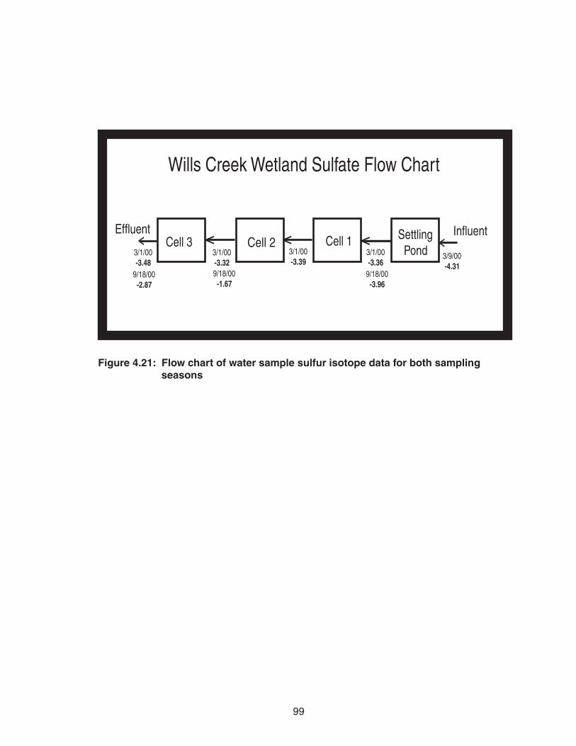
Cell 3 Cell 2 Cell 1 Settling Pond

> > >>

3/9/00 -4.31

3/1/00 -3.36

9/18/00 -3.96

9/18/00 -1.67

9/18/00 -2.87

Wills Creek Wetland Sulfate Flow Chart

> InfluentEffluent

3/1/00 -3.39

3/1/00 -3.32

3/1/00 -3.48

Figure 4.21: Flow chart of water sample sulfur isotope data for both sampling seasons

99

100

Wills Creek Wetland Native Sulfur/CrRS δ34S vs Distance Traveled

0

-27.63

-41.77

0

-36.06

-28.94

-6.1

-31.7

-31.11

-6.61

-45

-40

-35

-30

-25

-20

-15

-10

-5

0

WC cell 1 top WC cell 1 bottom WC cell 2 top WC cell 2 bottom WC cell 3

Sample Location

δ34S

CrRS Native Sulfur

Figure 4.22: Native sulfur and Cr Reduced sulfur isotopes for winter and summer

seasons versus distance traveled through the wetland

101

4.5 Simco Results and Interpretation

4.5.1 Introduction

The Simco constructed wetland in Zanesville, Ohio consists of 4 cells through

which AMD travels (Figure 2.7). This wetland has been very successful in treating AMD

since its construction in 1985. The success could be attributed to many factors including

regular monitoring and maintenance of the site, the type of compost used as a source for

organic carbon for the wetland, and the naturally high pH of the inlet waters. Because of

the long successful history of this wetland, it will be used as the standard with which to

compare the other four wetlands on the basis of water quality improvement. Acid mine

drainage enters the wetland system from underground coal mines into a holding pond,

from which water is distributed into cell 1 through a 3-foot wide channel and into cell 2

through a side channel that runs between cell 1 and an old high-wall. Effluent from cell 1

flows down a similar channel into a mixing pond, then into cell 3 where it meets and

mixes with effluent from cell 2. Effluent from cell 3 flows to cell 4 and out of the system

through an underground pipe that channels water to a series of settling ponds. These final

ponds were not designed to remediate AMD and were consequently excluded from our

study. Water flow through each of the cells is controlled by a series of weirs at the exits

of each cell and by straw bales strategically placed throughout the cells.


flow was noticed between cells and retention times and discharge rates were calculated.

Resulting calculations show that, on May 5th, 2000, Simco had a discharge of 2400


days. Rainfall data for May 2000 is shown graphically in Figure 4.23 and data collected

102

for August 2000 is shown in Figure 4.24. Minimal rainfall occurred before the May 11th

sampling with a suggesting that conditions at the time of sampling reflect normal

background conditions and not conditions that might exist due to abnormal precipitation.

August 24th data suggest significant rainfall occurred the day of sampling and several

days before sampling. This recent rainfall was still in the system based on retention time

calculations and may have influenced our field measurements, discharge calculations,

flow rates, and cell volume measurements.

Figure 4.23: May 2000 precipitation data showing minimal precipitation prior to the May 11th sampling

103

Figure 4.24: August 2000 precipitation data shows significant rainfall the day of sampling, affecting residence times and discharge calculations

4.5.2 Sampling

Simco was sampled in the winter and summer seasons of 2000, May 11th and

August 24th, and then again in the winter of 2001 on February 23rd. Water samples were

taken at the influent and effluent of each cell and side channel, and soil samples were

taken near the middle of each cell. Pore water samples were taken in winter 2001 in the

place of soil samples. However, pore water data is limited and no adequate interpretation

of the laboratory results can be made. All sampling locations are shown in the site map,

Figure 2.7. Field and laboratory data are shown in Tables 17, 18, 19, and 20. Influent

AMD to the system was measured in the holding pond as Sim-1 inlet. This influent also

enters cell 2 through the side channel and was measured as sample Sim-2 inlet. Effluent

from cell 1 and cell 2 were measured as Sim-1 outlet and Sim-2 outlet respectively. Sim-

1 outlet water flows through another side channel and into a mixing pond between cells 2

104

and 3 where it mixes with the flow from cell 2 outlet. The mixed water from cells 1 and

2 enters cell 3 and is measured as Sim-3 inlet. Effluent from cell 3 is measured as Sim-4

inlet and resulting wetland effluent as Sim-4 outlet. Soil samples were measured in the

holding pond and at the middle of every cell. Samples were taken at an approximate

depth of 6 inches and the top and bottom of the sample were analyzed.

4.5.2.1 Past Sampling and Interpretation

The Simco Wetland has been studied in great detail over its fifteen year life.

Lloyd R. Stark has published numerous papers on the wetland and selected data from his

previous studies are listed below in Table 16. The table shows mean water quality data

from February 1st, 1990 to March 1st, 1991.

Simco Previous Studies Parameter Inlet Outlet pH 6.68 +/- 0.12 6.93 +/- 0.14 Conductivity (MS/cm) 1.538 +/- 0.155 1.459 +/- 0.131 Acidity (mg/L) 147.6 +/- 22.3 29.5 +/- 4.8 Alkalinity (mg/L) 86.4 +/- 19.6 58.3 +/- 14.8 Sulfate (mg/L) 863 +/- 110 824 +/- 109 Total Fe (mg/L) 69.5 +/- 8.9 13.5 +/- 6.1 Total Mn (mg/L) 1.34 +/- 0.18 1.45 +/- 0.24

Table 16: Mean water quality data from the Simco wetland, February 1, 1990 to March 1, 1991. (from Stark 1951)

These measurements correspond very well to present day sampling data found in Tables

17, 18, and 19. Influent pH values have remained high since 1991 and conductivity

values are very similar to our field measurements. Sulfate concentrations shown in Table

16 are slightly higher than our findings but do fall from the inlet to the outlet of the

wetland, supporting our observation of sulfate concentration decline. Stark’s data also

105

corresponds well with our metal concentration data. Iron concentrations for both data

sets fall significantly with distance traveled through the wetland while manganese

concentrations remain constant or rise slightly. The fall in iron concentrations seen with

our recent data set suggest that the Simco wetland is still efficient at removing iron from

the system. However, influent iron concentrations have fallen from the 1990 / 1991 data

and corresponding effluent concentrations have fallen as well. There is a possible

correlation between the fall of influent iron concentrations and the fall of influent sulfate

concentrations. Possibly the source of AMD for the wetland is becoming depleted in

pollutants.

4.5.3 Water Samples



and sulfur isotope values and field measurements were taken for pH, Redox (mV), and

Conductivity. Conductivity with distance traveled through the wetland decreases slightly

during all seasons. Inlet pH for the system during winter 2000 was measured at 6.58

while effluent pH was measured at 6.62. Similar pH measurements were made during

summer 2000 and winter 2001, with the effluent pH measured at 7.26 during the summer

and 6.60 for the winter. pH remains relatively high throughout the system during every

sampling season and does not fluctuate drastically from cell to cell through the wetland.

For example, winter 2000 values fluctuate from a low value measured at Sim-3 inlet at

6.47 and the highest value measured at Sim-2 out and Sim-4 out at 6.62. These relatively

high pH values throughout the wetland provide ideal conditions for sulfate reducing

106

bacteria. Influent pH has consistently been high at Simco, one of the reasons for the

wetland’s continued success.


Sulfate concentrations, measured in ppm SO4, are plotted in Figure 4.25 versus

distance traveled through the wetland. Sulfate decreases slightly in the winter 2000

sampling from an influent concentration of 599 ppm to an effluent concentration of 542

ppm. Sulfate concentration is lowest at the outlet from cell 2 during winter 2000 but

resulting effluent from the wetland is not significantly lower than influent suggesting that

there is not a significant decrease in sulfate. The winter 2001 sampling shows the same

trend, with an influent concentration of 741 ppm and a corresponding effluent of 708

ppm. Lack of a significant decrease in sulfate concentrations suggest that sulfate

reduction is not occurring during the winter months at Simco. The summer 2000

sampling shows a greater decrease in sulfate concentrations, from an influent of 640 ppm

to an effluent of 290 ppm suggesting that sulfate reduction is occurring during the

summer season. Sulfur isotopes from the winter and summer support sulfate

concentration data.


Sulfur isotope data is shown in Table 18 and is also displayed in Figure 4.26 as a

simplified flow chart through each wetland cell. Figure 4.27 shows the change in

isotopic values for all three sampling seasons with distance traveled through the wetland.

The summer data shows a significant increase in δ34S , from a value of –3.58 for the inlet

107

sample to +6.26 from cell 4. The trend to a heavier δ34S value at the effluent suggests

that sulfate reduction is occurring at Simco during the summer. Winter season data

indicate just the opposite, with little change in the isotopic value from influent to effluent.

Winter 2000 data for the influent show a value of –3.88 while the effluent δ34S value was

–3.27. Winter 2001 data show similar trends, with an influent δ34S value of –4.06 and an

effluent value of –3.28. Both sets of winter isotope data suggest that sulfate reduction is

not an active process during the winter season at Simco. Thus, sulfate reduction appears

to be a seasonal process at Simco, relatively active during the summer season with clear

reduction trends in both isotope and sulfate concentration data, and relatively inactive

during the winter seasons with no clear trend of sulfate reduction.


Water samples were taken at the influent and effluent of the wetland during all

three sampling seasons to determine the change in metal concentrations. Resulting data

can be found in Table 19. Data shows that for all seasons, Fe concentrations fell

significantly from the influent to the effluent samples. For example, Fe concentrations

during the winter 2000 sampling were 28.5 ppm at the influent and 0.11 ppm at the

effluent. Similar trends are seen for the winter 2001 samples, with influent and effluent

concentrations of 33.46 ppm and 2.56 ppm respectively. However, during the summer

2000 sampling, influent concentrations were as low as effluent concentrations for both

winter months. Influent Fe was 3.5 ppm for summer 2000 while effluent concentrations

for winter 2001 were 2.56 ppm. These low summer concentrations imply that there is a

seasonal relationship between temperature and influent iron concentrations. The low

108

summer influent iron concentrations could be the result of bacterial sulfate reduction and

subsequent iron precipitation before introduction to the wetland system.

4.5.4 Soil Samples


% sulfur. All values can be found in Table 20. Figure 4.28 shows the trend of native

sulfur isotope values for samples from both 2000 seasons. The data suggest that sulfate

reduction is inactive during the winter 2000 season. This supports the conclusion of

inactive sulfate reduction from water samples. Isotope values remain relatively constant

from the influent to the effluent, with winter 2000 values of –41.68 at the influent to the

wetland and –41.64 at the effluent. A sulfate reduction trend would make these δ34S

values less negative with distance traveled. However, little change in δ34S is seen

suggesting that no significant sulfate reduction is occurring. Summer data also shows a

trend to lighter isotopes from influent to effluent, inconsistent with sulfate reduction

trends seen in water data during the summer season. However, recall that data from

substrate samples is much too variable to show reliable sulfate reduction trends. Water

samples provide more reliable sulfur isotope values and sulfate concentrations levels.

Thus, I conclude that sulfate reduction is occurring at Simco during the summer and is

simply not seen during the winter seasons.

4.5.5 Conclusion

Sulfate reduction appears to be an active process at Simco during the summer

season, based on sulfate concentrations and sulfur isotopes from water samples taken

109

summer 2000. Sulfate reduction doesn’t appear active during either winter sampling

season. Sulfur isotopes and sulfate concentrations for both winter seasons don’t change

significantly to indicate a sulfate reduction trends. Also important to note is that during

our winter 2000 sampling season, beavers had dammed up the wetland at the effluent

pipe from cell 4, causing water levels to rise by about 2 feet throughout the wetland.

Mixing of water from cell to cell likely occurred during this time and the homogeneity of

our data could be a direct reflection of this flooding. However, winter 2001 data was

collected without any evidence of flooding or damming and values are relatively similar

to winter 2000 data suggesting that, while beavers may have had an influence on our

winter 2000 data, the effect was small. Also, due to the high water levels, flow

measurements would have been unrepresentative of normal wetland conditions and were

not taken.

110

Simco Wetland Field Measurements 5/11/00 Water

Samples pH Redox (mV) Eh Cond (MS/cm)

Sim-1 inlet 6.58 @ 4.9C \ \ 1.457 Sim-1 out 6.55 @ 3.5C \ \ 1.352 Sim-2 inlet 6.55 @ 3.0C \ \ 1.476 Sim-2 out 6.62 @ 4.1C \ \ 1.424 Sim-3 inlet 6.47 @ 6.4C \ \ 1.207 Sim-4 inlet 6.61 @ 3.0C \ \ 1.389 Sim-4 out 6.62 @ 6.0C \ \ 1.295

8/24/00 Water Samples

pH Redox (mV) Eh Cond (MS/cm)

Sim-1 inlet 6.47 \ \ 1.01 Sim-1 out \ \ \ \ Sim-2 inlet \ \ \ \ Sim-2 out \ \ \ \ Sim-3 inlet 6.82 \ \ 0.787 Sim-4 inlet \ \ \ \ Sim-4 out [email protected] \ \ 0.629

2/28/01 Water Samples

pH Redox (mV) Eh Cond (MS/cm)

Sim-1 inlet 5.92 @ 6.6 C -18 182 1.49 Sim-1 out 6.40 @ 3.6 C 80 280 0.898 Sim-2 inlet 6.34 @ 5.6 C 18 218 0.983 Sim-2 out 6.57 @ 7.2 C 13 213 0.867 Sim-3 inlet 6.63 @ 6.6 C 19 219 0.921 Sim-4 inlet 6.74 @ 2.8 C 23 223 0.915 Sim-4 out 6.60 @ 2.6 C 75 275 0.931

Table 17: Simco water samples taken all three seasons

111

Simco Water Samples Simco Water


5/11/00 Dissolved

Sulfate (ppm) 8/24/00 δ34S

8/24/00 Dissolved

Sulfate (ppm) Sim-1 inlet -3.88 599 -3.58 640 Sim-1 out -2.99 595 \ \ Sim-2 in -4.01 542 \ \

Sim-2 out -3.47 498 \ \ Sim-3 inlet -3.62 610 -2.29 430 Sim-4 in -3.46 519 \ \

Sim-4 out -3.27 542 6.26 290

Simco Water Samples

2/2801 δ34S

2/2801 Dissolved

Sulfate (ppm) 2/2801 Pore Water δ34S

2/2801 Pore Water Sulfate

(ppm) Sim-1 inlet -4.06 741 / 5 Sim-1 out -3.57 775 / / Sim-2 in -3.22 736 / /

Sim-2 out -3.22 724 / / Sim-3 inlet -3.26 714 / / Sim-4 in -2.86 711 / /

Sim-4 out -3.28 708 / 42 Table 18: Simco water sample sulfur isotope and sulfate concentration data

Simco Metal Concentrations Sample Date Fe (ppm) Mn (ppm) Ca (ppm) Na (ppm) K (ppm) Mg (ppm)

Sim-1 inlet 5/11/00 28.5 0.83 749 98.7 5.8 33.8 Sim-4 out 5/11/00 0.11 1.09 607 93.7 6.2 32.0 Sim-1 inlet 8/24/00 3.50 0.55 540 82.4 5.2 26.6 Sim-4 out 8/24/00 0.13 0.11 262 72.7 5.7 21.6 Sim-1 inlet 2/28/01 33.46 1.07 130 119.4 4.7 35.1 Sim-4 out 2/28/01 2.56 0.90 122 109.9 4.6 33.6 Table 19: Simco influent and effluent metal concentrations

112

Simco Soil Samples 5/11/00 Soil

Samples Native Sulfur δ34S

Native Sulfur %

Chrome Reduced

Sulfur δ34S Cr Reduced

Sulfur %

Sim-inlet top 6" -41.68 0.2462 \ \ Sim-inlet bottom 6" -38.59 0.0355 \ \

Sim-1 top 6" -33.42 0.0346 \ 0.0166 Sim-1 bott -33.29 0.0723 \ 0.0095

Sim-2 top 6" -32.24 0.1307 -12.08 0.4302 Sim-2 bottom 6" -9.15 0.5174 \ 0.0459

Sim-3 top 6" -37.42 0.7361 \ \ Sim-3 bottom 6" -32.85 0.2804 \ \

Sim-4 top 6" -41.64 0.1377 \ \ Sim-4 bottom 6" -47.31 \ \ \


Native Sulfur δ34S

Native Sulfur %

Chrome Reduced

Sulfur δ34S Cr Reduced

Sulfur %

Sim-1 top -34.66 0.0698 \ \ Sim-1 top 6" -29.66 \ \ \

Sim-3 top -37.22 0.0350 \ \ Sim-4 mid -41.39 0.7165 \ \ Sim Cattail -11.14 0.0065 \ \ Sim Coal \ \ \ \

2/28/01 Porewater Sulfides

ZnS δ34S ZnS %

Sim-inlet / 0.0073 Sim-4 / 0.0109

Table 20: Simco soil sample sulfur isotope and % sulfur data

113

Simco Wetland PPM SO4 5/11/00 vs 8/24/00

599

498

610542

519

595542

775708

711741 736 714724

R2 = 0.204

R2 = 0.667

0

100

200

300

400

500

600

700

800

900

Sim-1 inlet Sim-1 out Sim-2 in Sim-2 out Sim-3 inlet Sim-4 in Sim-4 out

Sample Locations

PPM SO4

5/11/00 2/28/01

8/24/00

5/11/00

2/28/01640

430 290

8/24/00

Figure 4.25: Sulfate concentration trends for winter and summer 2000 and winter 2001 with distance traveled through the wetland

Cell 1

Cell 2

Cell 3

Cell 4

>

>

5/11/00 -2.99

2/28/01 -4.06

9/18/00 -2.29

9/18/00 -3.27

9/18/00 -3.58

>>

>>Influent

> >

>

>

>

>

Effluent

>

5/11/00 -4.01

5/11/00 -3.47

5/11/00 -3.62

5/11/00 -3.46

5/11/00 -3.27

Simco Wetland Sulfate Flow Chart

5/11/00 -3.88

2/28/01 -3.57

2/28/01 -3.22

2/28/01 -3.22

2/28/01 -3.26

2/28/01 -2.86

2/28/01 -3.28

Figure 4.26: Flow chart of water sample sulfur isotope data for all three sampling seasons

114

115

Simco Wetland Water Samples δ34S

-4.01-3.27

6.26

-3.46-3.62-3.47

-2.99

-3.88

-2.29

-3.58 -3.22 -3.26 -3.28

-4.06 -3.57

-3.22

R2 = 0.688

-6

-4

-2

0

2

4

6

8

Sim 1 inlet Sim 1 out Sim 2 in Sim 2 out Sim 3 inlet Sim 4 in Sim 4 out

Sample Locations

δ34S

5/11/00 8/24/00 2/28/01

5/11/00

8/24/00

2/28/01R2 = 0.509

Figure 4.27: Water sample sulfur isotopes for all seasons versus distance traveled through the wetland.

116

Figure 4.28: Native Sulfur isotope values versus distance traveled through the wetland

Simco 5/11/00 Soil SampleNative Sulfur δ34S vs Distance Traveled

-41.68

-33.42 -32.24

-41.64-37.42

-45

-40

-35

-30

-25

-20

-15

-10

-5

0

Sim-inlet top6" Sim-1 top 6" Sim-2 top 6" Sim-3 top 6" Sim-4 top 6"

Sample Locations

δ34S

117

Chapter 5: Discussion

Constructed wetland systems are designed to be an efficient, cost effective means

of remediating acid mine drainage replacing expensive, conventional chemical treatment

methods. The design of these wetlands involves building a wetland large enough to

accommodate the volume of influent AMD and promoting mixing of waters and

interaction with the substrate and vegetation. Each wetland varies in surface area,

volume, type of substrate used, and type of plant life incorporated. The five wetlands we

studied for this project were each unique in their approach to AMD treatment. Various

cell sizes within each wetland were used and various substrates and plant life were

incorporated. However, the goal of each wetland was the same: to improve water quality

from surrounding mines with minimum capital investment throughout the life of the

wetland. Although the goal was the same for each wetland, resulting effluents varied.

5.1 Wetland Sizing and Design

As discussed in Chapter 1, sizing of constructed wetlands is important to the long-

term effectiveness of AMD treatment. If the area of the cell is too small to provide

adequate retention of metals, the wetland substrate will reach equilibrium with respect to

these contaminants and metal precipitation will decrease. Thus, accurate influent AMD

water chemistry data is essential when designing and sizing future constructed wetlands.

I believe this to be the main problem at the Wills Creek wetland. Cell sizes were

designed too small to handle the enormous load of dissolved metals and sulfate entering

the system, and the wetland has seriously declined in treatment effectiveness.

118

5.2 Anoxic Limestone Drains

All of the wetland systems we studied, except the Simco wetland, begin with

influent waters passing through an anoxic limestone drain designed to boost the alkalinity

and pH of the AMD before it enters the wetland, creating ideal conditions for sulfate

reduction. The problem encountered at Tecumseh and Wills Creek involves clogging of

the ALD. Thus, influent waters must pass around the ALD and enter the wetland through

undesigned seeps. The water that bypasses the ALD doesn’t receive the initial boost of

alkalinity and pH that it normally would and the ideal conditions for sulfate reduction are

not created. At Wills Creek, one major seep has developed in the northeast corner of the

settling pond, providing an alternate route for AMD to enter the wetland. These seeps

adversely impact the performance of the wetland at removing sulfate and dissolved

metals from the system. Resulting effluent water quality reflects this poor performance.

Tecumseh has also developed a major seep in cell 4A, creating similar problems with

effluent water quality. The ALD at Midwestern does not appear to clogged, based on a

high influent pH. Thus, resulting effluent water chemistry reflects the quality of the

initial influent. Remediation processes at Midwestern are effective at improving water

quality because input parameters create ideal conditions for sulfate reduction. Therefore,

I conclude that the presence or absence of an effective ALD at the influent to a wetland

determines whether ideal conditions will be created to promote sulfate reduction and

water quality improvement.

Steps may be taken to insure the continued effectiveness of anoxic limestone

drains. One would be the replacement of the drain over a period of time determined by

individual AMD water chemistries and metal loading. Another suggestion would be to

119

use smaller limestone blocks in the drain. This would increase the surface area available

for influent water interaction and would prolong the life of the ALD because clogging

times would be longer. A third solution would be to use dolomite instead of limestone in

ALDs. This would slow the precipitation and coating of the drain by gypsum and prolong

the life of the ALD. Another method involves repetitive treatment by sand sized

limestone. Sand sized treatment of acid mine drainage streams has been documented by

Menendez (2000) to be an effective method for alkalinity generation and mine drainage

remediation. Results showed nearly complete dissolution of limestone and a significant

treatment of acid loads. Menendez (2000) suggests that monthly additions of limestone

sand may be sufficient for complete treatment of streams affected by acid mine drainage.

Whatever the solution, influent AMD must receive a boost of alkalinity and high pH to

insure that ideal conditions for sulfate reduction are created. However, the high cost of

repeated ALD maintenance may not be affordable and the current problems of clogged

drains may continue.

The utilization of anoxic limestone drains is not mandatory at all constructed

wetlands. The Simco wetland has a relatively neutral influent pH, 6.47 to 6.58, and high

concentrations of alkalinity (88 mg/L, Stark, 1995). Based on influent conditions, an

ALD was determined to be unnecessary at Simco. Influent conditions are adequate to

promote an environment suitable for sulfate reduction, and effluent water quality reflects

the quality of initial influents. Thus, the use of an ALD in the design of a given wetland

depends greatly on the initial water chemistry prior to construction.

120

5.3 Water Samples versus Soil Samples

Effluent water chemistry and wetland performance was determined by comparing δ34S

values for both water and soil samples. It was hoped that a thorough interpretation of

wetland performance could be made and that a distinct trend of sulfate reduction

throughout each wetland could be determined. However, high variability of δ34S for

substrate samples prevented such a comparison to be made. Water samples generated

δ34S values from which sulfate reduction trends were easily identified. Thus, water

samples seem to be the best medium with which to analyze sulfate reduction in wetlands.

Figure 5.1 below shows the variability of substrate samples compared to water samples

from the Tecumseh wetland. Values for the soil samples are spread throughout the

isotopic range and show no identifiable trend and a meager R2 value of 0.0931. Water

samples show an easily identifiable trend with a more correlative R2 value of 0.3579.

Thus, the water sample sulfur isotopes show a clearer trend of sulfate reduction during

the winter at Tecumseh while the soil samples show no clear trend. Wills Creek, Simco

and Friar Tuck wetland sulfur isotope data have similar correlation problems between soil

samples and water samples. The Midwestern wetland is the only wetland that shows a

fairly good correlation between soil and water samples. However, I believe that this

correlation is the exception rather the rule and have demonstrated that most substrate

samples are too variable in composition to provide an accurate δ34S value for sulfate

reduction analysis. Thus, on future wetland studies, water samples would be sufficient in

characterizing the processes occurring within the wetland.

121

Tecumseh Wetland δ34S Soil and Water Samples

vs Distance Traveled

Soil SamplesR2 = 0.0931

Water Samples R2 = 0.3579

-45

-40

-35

-30

-25

-20

-15

-10

-5

0

TCS-1 outlet TCS-2 outlet TCS-3 2ndberm

TCS-3 outlet TCS-4 outlet TCS-4A inlet TCS-4Amiddle

TCS-4Aoutlet

Sample Location

δ34S

Figure 5.1: Substrate samples show minimal correlation when compared with water samples.

5.4 Sulfate Reduction

The sulfate reduction trends seen in this study are indicative of one major

remediation process seen in constructed wetlands. The other main remediation method

has been simple mixing and dilution of the AMD. Sulfur isotopes from soil and water

samples has allowed me to determine whether sulfate reduction is occurring and is a

significant remediation process in the wetland. Field measurements and sulfate and metal

concentration values have also permitted me to make determinations of each wetlands

treatment performance. However, drops in sulfate and metal concentrations alone do not

prove that sulfate reduction is occurring in the wetland. Only an analysis of sulfur

122

isotope values and the fractionation seen from 32S to 34S can determine whether sulfate

reduction is a significant process in a wetland. An example involves data from the

Midwestern wetland. A significant drop in sulfate during the winter months is present

without a corresponding increase in δ34S. Thus, sulfate reduction is not a significant

treatment process during the winter months but sulfate water is still being removed,

possibly by the precipitation of gypsum. Therefore, because sulfate reduction isn’t

occurring in a wetland in a given season doesn’t necessarily mean that treatment of AMD

isn’t occurring.

5.5 Recommendations for Future Study

Rapid wetland analysis could be conducted simply by taking water samples at the

influent and effluent of the wetland and comparing field and laboratory data for each

sample. This would be a quick and effective way to determine instantaneous wetland

performance. Metal data taken for the wetlands that we studied show significant changes

in metal concentrations from influent to effluent, allowing interpretations of wetland

performance to be made with only two samples. Sulfate concentrations, pH, and sulfur

isotope trends could be determined from one influent and one effluent sample for each

wetland. However, this approach would limit the amount of interpretation that could be

made on wetland processes from cell to cell and prevent important findings within cells,

such as the additional AMD seeps found at Midwestern. It would also not discriminate

between simple dilution and sulfate reduction as the remediation process. A more

thorough comparison of wetlands would involve sampling the influent and effluent of the

wetland as well as the effluent from each cell within the wetland. It is not practical

123

however, to also utilize soil samples. Water samples are relatively simple to collect and

process and more data would be generated from which to draw conclusions about

wetland processes.

124

Chapter 6: References Bjorn, Christensen, Laake, Morten, Lien, Torleiv. 1996. Treatment of Acid Mine Water by Sulfate-Reducing Bacteria; Results From A Bench Scale Experiment. Wat.Res. Vol. 30, no 7, pp 1617 – 1624. Branam, Tracy, and Harper, Denver. Tabulated Analytical Data for Water Samples from the Friar Tuck Site. Final report to the Indiana Division of Reclamation Concerning Research and Reclamation Feasibility Studies at the Friar Tuck Site, Sullivan and Greene Counties, Indiana. Indiana Geological Survey Open-File Report 94-13, July 15, 1994. Brockmeyer, Frank. 1987 Investigation of Sources of Mine Drainage Pollution to Wills Creek Reservoir and their Impact on its Water Quality. A report from the special studies section, Abandoned Mined Lands Program, Division of Reclamation, Ohio Department of Natural Resources. Brodie, G.A., D.A. Hammer and D.A. Tomljanovich. 1988. Constructed wetlands for acid drainage control in the Tennessee Valley. In: Mine Drainage and Surface Mine Reclamation. Vol. 1: Mine Water and Mine Waste. Bureau of Mines IC 9183, Pittsburgh, PA. Bruchert, Volker, Pratt M., Lisa, Anderson F., Thomas, Hoffmann R., Stephen. 1995. Abuncance and Isotopic Composition of Organic and Inorganic Sulfur Species in Laminated and Bioturbated Sediments From Hole 893A, Santa Barbara Basin. Proceedings of the Ocean Drilling Program, Scientific Results, Vol. 146 (Pt. 2). Canfield, Donald E.; Raiswell, Robert; Westrich, Joseph T.; Reaves, Christopher M.; Berner, Robert A. 1986 The use of chromium reduction in the analysis of reduced inorganic sulfur in sediments and shales. Chemical Geology, 54, p 149-155. Cardamone, Milady A., Taylor, Jan R., Mitsch William, J., 1984 Wetlands and Coal Surface Mining: A Management Handbook. Research Report No. 154. University of Kentucky Water Resources Research Institute, Lexington, Kentucky. Agreement Number: G-844-23, P.L. 95-467. Childress, Chandra R. 1997. “Constructed Wetlands for the Treatment of Wastewater Containing Metals and Volatile Organic Compounds”. Masters Thesis, Department of Biology, College of Arts and Sciences, University of Cincinnati. Eddy, David P., Starck, Lloyd R., Stevens, S. Edward Jr., Webster, Harold J., Wenerick, William R., Williams, Frederick M. 1995. The Simco Constructed Wetland, A Final Report submitted to American Electric Power Service Corporation. Contract C-8161. Department of Biology and Wetland Research at Pennsylvania State University, University Park, PA 16802

125

Fauque, Guy D. 1995. Ecology of Sulfate-Reducing Bacteria. In Sulfate-Reducing Bacteria, edited by Larry L. Barton, Plenum Press, New York. Faure, Gunter. 1986. Principles of Isotope Geology, second edition. Harper, Denver, Olyphant, Greg. March 2000. Hydrology and Water Quality Associated with the Midwestern Reclamation Site (Site No. 1087), Pike County, Indiana. Indiana Geological Survey Project, http://adamite.igs.Indiana.edu/indsurv/research/projects/ Midwest/Midwest.html. Harrison, A.B. and H.G. Thode. 1957. The Kinetic Isotope Effect in the Chemical Reduction of Sulphate. Trans.Faraday Soc. 53, 1648. Hsu, Sophia C. 1998. The Use of Sulfur Isotopes to Determine the Effectiveness of Sulfate-Reduction in the Remediation of Acid Mine Drainage at Wills Creek Constructed Wetland. Masters Thesis, Dept of Geology, University of Cincinnati, College of Arts and Sciences. Hsu, Sophia C., Maynard, J.B., The Use of Sulfur Isotopes to Monitor the Effectiveness of Constructed Wetlands in Controlling Acid Mine Drainage. Environmental Engineering and Policy 1, 223-233. Kaplan, I.R. and Rittenberg, S.C. 1964. Microbiological Fractional of Sulphur Isotopes. J.gen.microbial. 34, 195 – 212. Kleinmann, R.L.P. 1989. Acid Mine Drainage: U.S. bureau of Mines researches and develops control methods for both coal and metal mines. Engineering and Mining Journal 190: 16I-16N. Kleinmann, R.L.P., R. Brooks, B. Huntsman, and B. Pesavento. 1986. Constructing Wetlands for the Treatment of Mine Water, Mini-Course Notes, 1986 National Symposium on Surface Mining, Hydrology, Sedimentology, and Reclamation. University of Kentucky, Lexington, KY. Kleinmann, R.L.P., and M.A. Girts. 1987. Acid mine water treatment in wetlands: an overview of an emergent technology. In: K.Reddy and H.Smith (eds.), Aquatic Plants for Water Treatment and Resource Recovery. Magnolia Publishing Co., Orlando, Florida. Knight, Robert L., Kadlec, Robert H., Wilhelm, Mel, Damgen, Francesca C., Gearheart, Robert A., Dyer, Jon C., Jackson, JoAnn, Shearer, John S. and staff, Richwine, Dale, newberry, Linda, Jockers, Mark. 1983. Constructed Wetlands for Wastewater Treatment and Wildlife Habitat: 17 Case Studies. United States Environmental Protection Agency EPA 832-R-93-005.

126

Menendez, Raymond, Clayton, Janet.L., Zurbuch, Peter E., Sherlock, Sean M., Rauch, Henry W., Renton, John J. 2000. Sand-Sized Limestone Treatment of Streams Impacted by Acid Mine Drainage. Water, Air, and Soil Pollution. Vol. 124: 411 – 428, 2000. Moore, Duane M. and Robert C. Reynolds, Jr. 1989. X-Ray Dffraction and the Identification and Analysis of Clay Minerals. Oxford University Press. Parkhurst, D.L. 1995 User’s guide to PHREEQC – a computer program for speciation, reaction-path, advective transport, and inverse geochemical calculations: U.S. Geological Survey Water-Resources Investigations Report 95-4227. Singleton, Jr. Rivers. 1993. The sulfate-reducing bacteria: An overview. In The Sulfate-Reducing Bacteria: Contemporary Perspectives, edited by J.M. Odom and Rivers Singleton, Jr. Springer-Verlag New York Inc. Skousen, J. 1991. Anoxic limestone drains for acid mine drainage treatment. Green Lands 21:30-35. Smith, A.J. 1989. Wastewaters: a perspective. P3-4 in D.A. Hammer (ed.), Constructed Wetlands for Wastewater Treatment. Lewis Publishers, Inc., Chelsea, MI. Smith, Ronald T, An Investigation of Toxic Metals Removal in AMD Treatment Wetlands. Proposal submitted to the Indiana Division of Reclamation Surface Mining and Reclamation Technology Grant Program, 2000. [email protected] Stark, L. R., R. L. Kolbash, H. J. Webster, S. E. Stevens, Jr., K. A. Dionis, and E.R. Murphy. 1988. The Simco #4 Wetland: Biological patterns and p erformance of a wetland receiving mind drainage. In: Mine Drainage and Surface Mine Reclamation. Vol. 1: Mine Water and Mine Waste. Bureau of Mines Information Circular 9183, Pittsburg, PA. Stark, L.R., Stevens, S. Edward Jr., Webster, Harold J., and Wenerick, William R. 1990. Iron Loading, Efficiency and Sizing in A Constructed Wetland Receiving Mine Drainage. In: Proceedings of the 1990 Mining and Reclamation Conference and Exhibiiton, Charleston, West Virginia, April 23 – 26, 1990. 2 Vols. West Virginia University, Morgantown, WV. Stark, L. R., F. M. Williams, S.E. Stevens, Jr., and D.P. Eddy. 1994. Iron Retention and Vegetative Cover at the Simco Constructed Wetland: an appraisal through year eight of operation. In: Proceedings, International Land Reclamation and Mine Drainage Conference and Third International Conference on the Abatement of Acidic Drainage, Vol. 1: Mine Drainage. Pittsburgh, PA. Stark, Lloyd R., Williams, Frederick M., Stevens, S. Edward Jr., Webster, Harold J., Wenerick, William R., Eddy, David P. 1995. The Simco Constructed Wetland: A Final Report Submitted to American Electric Power Service Corporation. Contract C-8161.

127

Standard Methods for the Examinaiton of Water and Wastewater. 1971. 13th ed. Stumm, W. and Morgan, J.J. 1981. Aquatic Chemistry, 2nd edition. Wiley Interscience, New York, 780 pp.

12

8

App

endi

x A

– W

eigh

t % C

arbo

n an

d Su

lfur

LEC

O A

naly

sis

Will

s C

reek

Mid

wes

tern

Sam

ple

%

Car

bon

%

Sulfu

r C

/S

Rat

io

Sam

ple

%

Car

bon

%

Sulfu

r C

/S

Rat

io

WC

cel

l1 to

p 3/

9 14

.95

1.66

7 8.

97

MW

S 1B

top

3/1

4.31

4 1.

405

3.07

W

C c

ell1

bot

t 3/9

Coa

ly

22.3

5 0.

7616

29

.35

MW

S 2A

3/1

Coa

ly

4.00

7 0.

4304

9.

31

WC

cel

l1 b

ott C

r 3/9

44

.42

1.40

7 31

.57

MW

S 2B

2 3/

1 C

oaly

6.

902

0.87

46

7.89

W

C c

ell2

top

3/9

Coa

ly

6.52

9 0.

6173

10

.58

MW

S 2B

3 3/

1 C

oaly

3.

44

0.60

02

5.73

W

C c

ell2

Cr 3

/9

6.89

2 0.

0878

8 78

.43

MW

S 2C

1 3/

1 3.

163

0.58

17

5.44

W

C c

ell2

top

Cr 3

/9

5.42

5 0.

1085

50

.00

MW

S 2C

7 3/

1 1.

051

0.48

87

2.15

W

C c

ell3

Cr 3

/9

19.0

2 0.

6939

27

.41

MW

S 2A

9/1

8 C

oaly

3.

489

0.52

62

6.63

W

C c

ell 1

8/2

4 11

.84

2.09

3 5.

66

MW

S 2B

2 m

id 9

/18

5.92

2 1.

572

3.77

W

C c

ell2

8/2

4 17

.58

2.11

8 8.

30

MW

S 2B

3 9/

18

3.07

1 0.

3013

10

.19

WC

cel

l3 8

/24

1.41

6 0.

2526

5.

61

MW

S 2C

7 9/

18

1.00

8 0.

3877

2.

60

WC

Coa

l 62

.82

1.52

3 41

.25

MW

S C

oal

65.8

4 2.

152

30.5

9 W

C C

atta

il 39

.56

0.05

638

701.

67

MW

S C

atta

il 36

.59

0.16

44

222.

57

12

9

Sim

co

Te

cum

seh

Sa

mpl

e %

C

arbo

n %

Su

lfur

C/S

R

atio

Sa

mpl

e %

C

arbo

n %

Su

lfur

C/S

R

atio

Si

m in

let b

ott 5

/11

4.22

1 0.

1422

29

.68

TCS

1 ou

t 3/1

2.

701

0.32

13

8.41

Si

m c

ell1

top

5/11

3.

907

0.21

66

18.0

4 TC

S1 o

ut C

r 3/1

3.

505

0.05

362

65.3

7 Si

m c

ell1

bot

t 5/1

1 2.

373

0.10

17

23.3

3 TC

S 2

out 3

/1

3.98

1.

472

2.70

Si

m 1

top

Cr

5/11

Coa

ly

3.47

1 0.

0885

9 39

1.80

TC

S 2

out C

r 3/1

1.

794

0.06

132

29.2

6

Sim

1 b

ott C

r 5/1

1 1.

588

0.04

461

35.6

0 TC

S 3

out 3

/1

4.41

9 0.

4926

8.

97

Sim

cel

l2 to

p 5/

11

4.55

6 0.

4365

10

.44

TCS3

out

Cr 3

/1

3.04

3 0.

0738

4 41

.21

Sim

cel

l2 b

ott 5

/11

5.15

9 0.

3359

15

.36

TCS

3 2n

d be

rm 3

/1

6.43

1 0.

4033

15

.95

Sim

2 to

p C

r 5/1

1 8.

449

0.21

41

39.4

6 TC

S3 2

nd b

erm

Cr 3

/1

2.01

4 0.

0498

5 40

.40

Sim

2 b

ott C

r 5/1

1 7.

155

0.12

12

59.0

3 TC

S 4

out 3

/1

7.03

9 0.

5352

13

.15

Sim

cel

l3 to

p 5/

11

9.14

0.

4704

19

.43

TCS

4 ou

t Cr 3

/1

2.71

2 0.

0626

2 43

.31

Sim

cel

l3 b

ott 5

/11

7.34

1 2.

374

3.09

TC

S 4A

inle

t 3/1

1.

117

0.67

33

1.66

Si

m c

ell4

top

5/11

10

.42

0.59

17

.66

TCS

4A m

id 3

/1

7.18

6 0.

3765

19

.09

Sim

cel

l 4 b

ott 5

/11

21.6

4 1.

268

17.0

7 TC

S 4A

out

3/1

2.

975

0.28

26

10.5

3 Si

m c

ell3

8/2

4 3.

422

0.20

45

16.7

3 TC

S 4A

inle

t Cr 3

/1

1.55

2 0.

0416

8 37

.24

Sim

Coa

l 67

.21

3.90

3 17

.22

TCS

4A m

id C

r 3/1

2.

026

0.05

93

34.1

7 Si

m C

atta

il 39

.53

0.06

96

567.

96

TCS4

A ou

t Cr 3

/1

1.90

1 0.

0473

3 40

.16

TCS

2 ou

t 0-5

9/1

9 4.

019

1.02

4 3.

92

Fria

r Tuc

k

TCS

2 ou

t 5-1

0 9/

19

4.06

9 0.

8456

4.

81

Sam

ple

% C

arbo

n %

Sul

fur

C/S

Rat

io

TCS

4 ou

t 0-5

9/1

9 2.

039

0.23

74

8.59

FT

S 2

2/29

1.

083

0.38

33

2.83

TC

S 4

out 5

-10

9/19

1.

724

0.42

64

4.04

FT

S 2

Cr 2

/29

1.81

9 0.

0416

5 43

.67

TCS

4A in

let 0

-5 9

/19

1.90

4 0.

7914

2.

41

FTS

2A 2

/29

2.24

3 0.

2643

8.

49

TCS

4A in

let 5

-10

9/19

1.

633

0.56

21

2.91

FT

S 2A

Cr 2

/29

1.93

9 0.

0452

42

.90

TCS

4A o

ut 0

-5 9

/19

2.06

2 0.

6504

3.

17

Mus

h C

om N

S 27

.99

0.48

46

57.7

6

M

ush

Com

p C

r 18

.71

0.22

46

83.3

0

C

ow M

anur

e N

S 29

.05

0.39

84

72.9

2

C

ow M

anur

e C

r 33

.31

0.09

212

361.

59

13

0

App

endi

x B

– X

-ray

Flu

ores

cenc

e D

ata

XRD

Dat

a

ppm

pp

m

ppm

pp

m

ppm

%

%

pp

m

ppm

%

pp

m

Wet

land

s

U

Pb

Zn

Cu

Ni

Fe2O

3 M

nO

Cr

V Ti

O2

Ba

FTS2

2/

29/0

0 3.

7 20

.5

118

22

51

5.34

0.

049

73

95

1.07

51

0 FT

S2A

2/29

/00

4.3

21.3

90

24

38

3.

69

0.06

5 10

7 84

1.

06

510

MW

S 1B

3/1/

00

8.6

27.3

21

4 76

89

6.

69

0.09

6 82

13

9 0.

96

420

MW

S 2A

3/1/

00

8.3

25.8

14

5 49

51

6.

65

0.06

3 97

18

8 1.

10

500

MW

S 2A

9/

18/0

0 7.

2 24

.7

149

42

58

7.47

0.

046

122

174

1.09

51

0 M

WS

2B2

9/

18/0

0 6.

5 17

.7

242

51

478

8.61

0.

185

142

131

0.92

44

0 M

WS

2B3

3/1/

00

5.6

23.5

17

9 77

56

7.

36

0.14

5 10

7 13

7 1.

07

490

MW

S 2C

1

3/

1/00

7.

3 29

.1

113

39

43

7.44

0.

051

131

175

1.09

54

0 M

WS

2C2

3/1/

00

3.2

60.4

61

3 46

4 17

2 4.

14

0.33

1 10

7 76

0.

66

540

MW

S 2C

3

3/

1/00

4.

8 25

.3

125

35

47

7.63

0.

077

106

157

1.11

51

0 M

WS

2C4

3/1/

00

4.1

15.7

33

1 21

8 69

3.

89

0.13

4 62

89

0.

87

350

MW

S 2C

5

3/

1/00

2.

6 16

.3

202

154

27

3.96

0.

058

49

86

0.87

37

0 M

WS

2C6

3/1/

00

3.3

17.4

82

15

39

3.

90

0.06

3 78

98

1.

08

360

MW

S 2C

7

3/

1/00

3.

2 26

.6

90

19

32

6.48

0.

038

108

158

1.21

47

0

13

1

ppm

pp

m

ppm

pp

m

ppm

%

%

pp

m

ppm

%

pp

m

Wet

land

s

U

Pb

Zn

Cu

Ni

Fe2O

3 M

nO

Cr

V Ti

O2

Ba

SIM

inle

t bot

tom

3 in

5/

11/0

0 0.

8 12

.3

85

2 24

24

.54

0.12

9 11

2 12

1 0.

99

420

SIM

IN

5/11

/00

0.9

5.4

50

b.d.

9

44.1

8 0.

080

49

78

0.62

28

0 SI

M 1

bot

tom

3 in

5/

11/0

0 3.

9 26

.4

69

25

34

9.64

0.

029

202

156

1.36

45

0 SI

M 1

top

3 in

5/

11/0

0 3.

0 19

.1

49

4 18

22

.72

0.04

2 10

4 14

0 1.

19

420

SIM

2 to

p 3

in

5/11

/00

0.8

5.4

26

b.d.

b.

d.

46.6

5 0.

036

60

84

0.70

25

0 SI

M 3

bot

tom

3 in

5/

11/0

0 1.

6 1.

7 17

0 b.

d.

142

53.8

6 0.

080

16

18

0.11

60

SI

M 3

top

3 in

5/

11/0

0 0.

3 2.

7 64

b.

d.

116

57.8

7 0.

102

6 11

0.

06

130

SIM

4 b

otto

m 3

in

5/11

/00

1.9

12.5

28

7 58

11

7 18

.02

0.05

7 42

55

0.

38

220

SIM

4 to

p 3

in

5/11

/00

2.7

11.4

65

9

63

29.1

8 0.

086

86

106

0.90

35

0

TC

S 1

OU

T

3/1/

00

4.3

24.3

14

3 78

30

4.

17

0.08

1 74

81

0.

97

410

TCS

2 O

UT

9/19

/00

2.3

4.3

65

10

6 33

.29

0.07

2 68

79

0.

70

270

TCS

3 2n

d be

rm

9/19

/00

2.9

24.7

11

8 74

28

4.

56

0.06

4 18

8 78

0.

99

410

TCS

4 O

UT

9/19

/00

5.0

21.7

18

8 48

26

4.

99

0.02

9 11

4 89

1.

03

410

TCS

4A in

3/

1/00

5.

6 22

.2

107

29

29

8.35

0.

027

204

125

1.13

51

0 W

C1

8/

24/0

0 3.

4 22

.3

778

47

533

14.3

9 0.

045

76

100

0.69

42

0 W

C2

low

er s

ectio

n 3/

9/00

3.

9 20

.1

83

19

29

7.88

0.

031

85

113

1.03

49

0 W

C 3

3/

9/00

2.

7 11

.0

250

5 10

1 19

.70

0.14

6 10

8 10

5 0.

80

390

13

2

App

endi

x C

W

ater

Che

mis

try/

Met

al C

once

ntra

tion

Dat

a

Wat

er C

hem

istr

y D

ata

Fria

r Tuc

k 2/

29/0

0 A

cidi

ty

(mg/

L)

Alk

alin

ity

(mg/

L)

Fe2+

(m

g/L)

SO

42-

(mg/

L)

HC

O3-

(mg/

L)

Cl (

mg/

L)

FTS

inle

t 30

17

3 0

1300

21

0 2.

8 FT

S 2

6220

0

1564

13

,000

0

<5.0

0 FT

S 2A

32

13

2 50

12

52

160

2.2

FTS

3 34

85

0.

1 93

0 10

0 2.

1

Mid

wes

tern

3/

1/00

A

cidi

ty

(mg/

L)

Alk

alin

ity

(mg/

L)

Fe2+

(m

g/L)

SO

42-

(mg/

L)

HC

O3-

(mg/

L)

Cl (

mg/

L)

MW

S 1A

inle

t 17

1 0

45

2270

0

17.1

M

WS

1A o

ut

122

0 68

17

20

0 10

.4

MW

S 2A

35

18

8 0.

1 14

50

230

15.4

M

WS

2B2

36

158

0 12

68

190

13.8

M

WS

2B3

40

17

0.4

1130

20

21

M

WS

2C2

26

42

0.1

1160

50

23

M

WS

2C7

15

76

0 76

5 90

12

Tecu

mse

h 3/

1/00

A

cidi

ty

(mg/

L)

Alk

alin

ity

(mg/

L)

Fe2+

(m

g/L)

SO

42-

(mg/

L)

HC

O3-

(mg/

L)

Cl (

mg/

L)

TCS

1 ou

t 22

12

3 1.

5 15

22

150

4.9

TCS

2 ou

t 24

84

1

1608

10

0 4.

9 TC

S 4A

out

13

04

0 54

7 33

58

0 2.

1 TC

S 4

out

27

111

0 15

20

140

4.5

TCS

5 ou

t 18

82

0

1442

10

0 4.

5

13

3

Wat

er C

hem

istr

y D

ata

Will

s C

reek

Fe

(p

pm)

Mn

(p

pm)

Ca

(ppm

) N

a (p

pm)

K

(ppm

) M

g

(ppm

)

WC

cel

l 1 in

let 5

/11/

00

12.6

8.

45

949

27.6

6

49.9

WC

cel

l 3 o

ut 5

/11/

00

4.2

7.91

99

6 27

.6

7.4

49.4

WC

cel

l 1 in

let 8

/24/

00

10.1

6.

72

983

35.9

6.

5 46

.2

W

C c

ell 3

out

8/2

4/00

4.

3 6.

9 10

68

28.2

10

44

.7

Sim

co

Fe

(ppm

) M

n

(ppm

) C

a (p

pm)

Na

(ppm

) K

(p

pm)

Mg

(p

pm)

Sim

1 In

let 5

/11/

00

28.5

0.

83

749

98.7

5.

8 33

.8

Si

m 4

out

5/1

1/00

0.

11

1.09

60

7 93

.7

6.2

32

Si

m 1

Inle

t 8/2

4/00

3.

5 0.

55

540

82.4

5.

2 26

.6

Si

m 4

out

8/2

4/00

0.

13

0.11

26

2 72

.7

5.7

21.6

Sim

co

2/

28/0

1 Fe

(p

pm)

Mn

(p

pm)

Ca

(ppm

) N

a (p

pm)

K

(ppm

) M

g

(ppm

) C

l (p

pm)

SO4

(ppm

) A

l (p

pm)

Sim

1 in

let

33.4

6 1.

065

129.

84

119.

37

4.69

35

.11

114.

04

615.

03

0.59

2 Si

m 1

out

0.

61

1.11

2 13

5.88

12

2.33

4.

95

36.8

8 14

6.38

64

6.44

0.

211

Sim

2 in

let

19.2

8 1.

013

125.

37

112.

88

4.55

34

.25

161.

7 62

4.01

<0

.2

Sim

2 o

ut

16.1

2 1.

013

128.

34

116.

07

4.47

35

.21

129.

36

613.

38

<0.2

Si

m 3

inle

t 10

.28

0.96

1 12

3.2

112.

59

4.35

33

.76

144.

68

590.

23

<0.2

Si

m 3

out

6.

23

0.91

12

2.84

11

1.85

4.

87

33.7

15

4.89

58

8.5

<0.2

Si

m 4

out

2.

56

0.90

2 12

2.42

10

9.86

4.

55

33.6

18

0.42

58

0.24

0.

229

13

4 A

ppen

dix

D –

X-r

ay D

iffra

ctog

ram

Dat

a

135

136

137

138

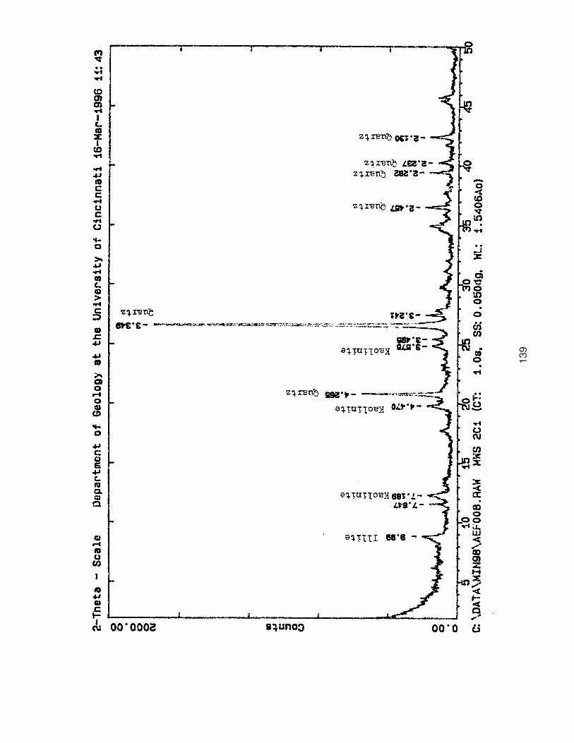
139

140

141

142

143

144

145

146

Appendix E – PHREEQC

TITLE Saturation of Gypsum at MWS 2C7 SOLUTION 1 Acid Mine Drainage units ppm pH 7.34 temp 10.6 Ca 323.04 Mg 102.90 Na 24.82 K 11.84 Fe 3.4 Mn 5.391 Cl 241.69 Alkalinity 90.0 as HCO3 S(6) 831.0 END

Log Log Log Species Molality Activity Molality Activity Gamma CaSO4 1.733e-03 1.747e-03 -2.761 -2.758 0.004 Phase SI log IAP log KT Gypsum -0.14 -5.00 -4.59 CaSO4:2H2O TITLE Saturation of Gypsum at MWS 2C2 SOLUTION 1 Acid Mine Drainage units ppm pH 6.31 temp 13.6 Ca 323.04 assumed same as 2C7 Mg 102.90 assumed same as 2C7 Na 24.82 assumed same as 2C7 K 11.84 assumed same as 2C7 Fe 3.4 Mn 5.391 assumed same as 2C7 Cl 241.69

Alkalinity 50.0 as HCO3 S(6) 1170.0 END

Log Log Log Species Molality Activity Molality Activity Gamma CaSO4 2.318e-03 2.338e-03 -2.635 -2.631 0.004 Phase SI log IAP log KT Gypsum -0.04 -4.88 -4.59 CaSO4:2H2O

147

TITLE Saturation of Gypsum at MWS 2B3 SOLUTION 1 Acid Mine Drainage units ppm pH 5.48 temp 12.1

Ca 543.95 1B Mg 220.73 1B Na 24.16 1B K 7.68 1B Fe 101.73 1B Mn 13.677 1B Cl 175.31 1B Alkalinity 20.0 as HCO3 S(6) 1210.0 END

Log Log Log Species Molality Activity Molality Activity Gamma CaSO4 2.893e-03 2.931e-03 -2.539 -2.533 0.006 Phase SI log IAP log KT Gypsum +0.07 -4.78 -4.59 CaSO4:2H2O TITLE Saturation of Gypsum at MWS 2B2 SOLUTION 1 Acid Mine Drainage units ppm pH 6.41 temp 13.1

Ca 543.95 1B Mg 220.73 1B Na 24.16 1B K 7.68 1B Fe 101.73 1B Mn 13.677 1B Cl 175.31 1B Alkalinity 190.0 as HCO3 S(6) 1230.0 END

Log Log Log Species Molality Activity Molality Activity Gamma CaSO4 2.918e-03 2.957e-03 -2.535 -2.529 0.006 Phase SI log IAP log KT Gypsum +0.07 -4.78 -4.59 CaSO4:2H2O

148

TITLE Saturation of Gypsum at MWS 2A SOLUTION 1 Acid Mine Drainage units ppm pH 7.21 temp 16.5 Ca 543.95 1B Mg 323.04 1B Na 24.16 1B K 7.684 1B Fe 101.73 1B Mn 13.677 1B Cl 175.31 1B Alkalinity 230.0 as HCO3 S(6) 1350.0 END

Log Log Log Species Molality Activity Molality Activity Gamma CaSO4 2.908e-03 2.952e-03 -2.536 -2.530 0.006 Phase SI log IAP log KT Gypsum +0.09 -4.80 -4.58 CaSO4:2H2O

Documents

UNIVERSITY OF CINCINNATI - UCFileSpace Tools - Homehomepages.uc.edu/~maynarjb/Frontpage sites/Research/s/Ada… · B.S. University of Cincinnati ... The Simco wetland was flooded