UNIVERSITY OF CALIFORNIA, SAN DIEGO

Simultaneous Regression and Clustering to Predict Movie Ratings

A thesis submitted in partial satisfaction of therequirements for the degree

Master of Science

in

Computer Science

by

Matthew Rodriguez

Committee in charge:

Professor Charles Elkan, ChairProfessor Roger LevyProfessor Lawrence Saul

2010

Copyright

Matthew Rodriguez, 2010

All rights reserved.

The thesis of Matthew Rodriguez is approved, and it is ac-

ceptable in quality and form for publication on microfilm and

electronically:

Chair

University of California, San Diego

2010

iii

TABLE OF CONTENTS

Signature Page . . . . . . . . . . . . . . . . . . . . . . . . . . . . . . . . . . . iii

Table of Contents . . . . . . . . . . . . . . . . . . . . . . . . . . . . . . . . . . iv

List of Figures . . . . . . . . . . . . . . . . . . . . . . . . . . . . . . . . . . . . vi

List of Tables . . . . . . . . . . . . . . . . . . . . . . . . . . . . . . . . . . . . vii

Acknowledgements . . . . . . . . . . . . . . . . . . . . . . . . . . . . . . . . . viii

Vita and Publications . . . . . . . . . . . . . . . . . . . . . . . . . . . . . . . . ix

Abstract of the Thesis . . . . . . . . . . . . . . . . . . . . . . . . . . . . . . . . x

Chapter 1 Introduction . . . . . . . . . . . . . . . . . . . . . . . . . . . . . 1

Chapter 2 Performing Logistic Regression on the Movielens dataset . . . . . 32.1 Background . . . . . . . . . . . . . . . . . . . . . . . . . . 32.2 Selection of the Training Examples . . . . . . . . . . . . . . 32.3 Feature Selection of the Logistic Model . . . . . . . . . . . 52.4 Logistic Regression Experiments . . . . . . . . . . . . . . . 9

Chapter 3 Overview of the Predictive Discrete Latent Factor model . . . . . 133.1 Background . . . . . . . . . . . . . . . . . . . . . . . . . . 133.2 Generalized Linear Models and Exponential Families . . . . 133.3 Predictive Discrete Latent Factor Model . . . . . . . . . . . 153.4 Fitting the PDLF Model . . . . . . . . . . . . . . . . . . . 17

Chapter 4 Using a Bernoulli as the Exponential Family Member in a PDLFModel . . . . . . . . . . . . . . . . . . . . . . . . . . . . . . . . 214.1 Background . . . . . . . . . . . . . . . . . . . . . . . . . . 214.2 Bernoulli Distribution . . . . . . . . . . . . . . . . . . . . . 214.3 Optimization . . . . . . . . . . . . . . . . . . . . . . . . . 224.4 Experiments . . . . . . . . . . . . . . . . . . . . . . . . . . 234.5 Analysis . . . . . . . . . . . . . . . . . . . . . . . . . . . . 25

Chapter 5 Using a Multinomial as the Exponential Family Member in a PDLFModel . . . . . . . . . . . . . . . . . . . . . . . . . . . . . . . . 295.1 Background . . . . . . . . . . . . . . . . . . . . . . . . . . 295.2 Using a GLM for a Multinomial distribution . . . . . . . . . 30

5.2.1 Algorithm Implementation . . . . . . . . . . . . . . 305.2.2 Optimization . . . . . . . . . . . . . . . . . . . . . 31

iv

5.2.3 Testing the Model’s Implementation . . . . . . . . . 325.3 Testing the Regression Coefficients . . . . . . . . . . . . . . 335.4 Testing the Interaction Effects . . . . . . . . . . . . . . . . 355.5 Testing the multinomial PDLF model . . . . . . . . . . . . 36

5.5.1 Annealing to improve coclustering . . . . . . . . . . 395.5.2 Soft clustering approach . . . . . . . . . . . . . . . 415.5.3 Analysis of the soft clustering model . . . . . . . . . 455.5.4 Cocluster initialization by sorting . . . . . . . . . . 46

5.6 Comparison between the Bernoulli and multinomial models 48

Chapter 6 Conclusions . . . . . . . . . . . . . . . . . . . . . . . . . . . . . 49

Bibliography . . . . . . . . . . . . . . . . . . . . . . . . . . . . . . . . . . . . 50

v

LIST OF FIGURES

Figure 2.1: Histograms of the frequency of user ratings and movie ratings . . . 4Figure 2.2: Precision for each feature versus rating in the first and second fea-

ture sets . . . . . . . . . . . . . . . . . . . . . . . . . . . . . . . . 9Figure 2.3: Log likelihood during training of the logistic models . . . . . . . . 10

Figure 4.1: Value of clustering objective functions at each iteration . . . . . . . 24Figure 4.2: Number of changes in clustering assignments . . . . . . . . . . . . 24Figure 4.3: Regression coefficients of the trained PDLF model . . . . . . . . . 25Figure 4.4: Training and testing Bernoulli parameters for one fold . . . . . . . 26Figure 4.5: Values of the objective functions for the regression coefficients and

interaction effects and the log likelihood versus iteration . . . . . . 27Figure 4.6: Hinton diagrams of cocluster assignments and interaction effects . . 28

Figure 5.1: Derivation of the gradient for the regression coefficients . . . . . . 32Figure 5.2: Derivation of the gradient for the interaction effects . . . . . . . . . 33Figure 5.3: The result of the objective function, MSE and log likelihood during

training the model using only regression coefficients . . . . . . . . 34Figure 5.4: Predictions and absolute prediction error using regression coefficients 35Figure 5.5: Regression coefficients . . . . . . . . . . . . . . . . . . . . . . . . 36Figure 5.6: The result of the objective function, MSE, and log likelihood during

training the model using only interaction effects . . . . . . . . . . . 37Figure 5.7: Change in coclustering assignments using interaction effects . . . . 37Figure 5.8: Histogram of predictions and absolute error using interaction effects 38Figure 5.9: MSE and log likelihood during training of the hard clustering PDLF

model . . . . . . . . . . . . . . . . . . . . . . . . . . . . . . . . . 39Figure 5.10: Histogram of predictions and absolute error on training data . . . . 40Figure 5.11: Hinton diagrams of regression coefficients and interaction effects of

the hard clustering PDLF model . . . . . . . . . . . . . . . . . . . 40Figure 5.12: Coclustering assignments using different variations of the coclus-

tering algorithm or pdlf model . . . . . . . . . . . . . . . . . . . . 41Figure 5.13: Number of cocluster assignments changes at each iteration using

PDLF coclustering algorithm . . . . . . . . . . . . . . . . . . . . . 42Figure 5.14: Number of cocluster assignments changes at each iteration when

using the annealing coclustering algorithm . . . . . . . . . . . . . 42Figure 5.15: MSE and log likelihood during training of the soft clustering PDLF

model . . . . . . . . . . . . . . . . . . . . . . . . . . . . . . . . . 46Figure 5.16: Mixture component priors and interaction effects of the soft cluster-

ing PDLF model . . . . . . . . . . . . . . . . . . . . . . . . . . . 46Figure 5.17: Hinton diagram of cocluster membership and histogram of predic-

tion for the multinomial model with cocluster initialization . . . . . 47

vi

LIST OF TABLES

Table 2.1: Table of features selected by stepwise regression . . . . . . . . . . . 6Table 2.2: Misclassification versus learning rate using first feature set . . . . . 11Table 2.3: Misclassification versus learning rate using the second feature set . . 11Table 2.4: Misclassification versus learning rate using the third feature set . . . 12Table 2.5: Misclassification versus learning rate using the fourth feature set . . 12

Table 4.1: Misclassification rate using different number of coclusters . . . . . . 25

Table 5.1: Zero/One misclassification rates for the multinomial models . . . . . 48

vii

ACKNOWLEDGEMENTS

Thank you to Charles Elkan and Aditya Menon for guiding me throughout this

process. Thank you to Lawrence Saul and Roger Levy for teaching me in their courses

and being on my Master’s Thesis committee. Thank you to Ilya Zaslavsky for helping

me get my Master’s.

viii

VITA

2001 B. S. in Electrical Engineering and Computer Science, Universityof California Berkeley

2007-2009 Graduate Student Researcher, University of California, San Diego

2010 M. S. in Computer Science, University of California, San Diego

ix

ABSTRACT OF THE THESIS

Simultaneous Regression and Clustering to Predict Movie Ratings

by

Matthew Rodriguez

Master of Science in Computer Science

University of California, San Diego, 2010

Professor Charles Elkan, Chair

A recommender system uses information from a user’s past behavior to present

items of interest to him. A fundamental problem in recommender systems is approxi-

mating a full user-item matrix where most of the entries are missing. The rows of the

matrix represent the users and the columns represent the items. The entries indicate the

plausibility that the user will enjoy the item. In this thesis the items are movies and the

entries ratings.

In this thesis I compare three statistical models that how a user will rate a movie.

The first two are Bernoulli models that predict whether a rating is greater than three out

of five. The first Bernoulli model uses logistic regression. The second Bernoulli model

is a latent factor model. The third model extends the latent factor model to use a five

class multinomial. A five class multinomial is chosen to predict a rating on a scale of

one to five.

The results show that latent factor model that uses a Bernoulli distribution has

a better accuracy than a model trained by logistic regression. The latent factor model

is extended to use a multinomial. The accuracy of variants of the multinomial model

are evaluated. A technique to initialize the multinomial model is shown to improve

x

the accuracy. However the accuracy is lower than other models used in the Netflix

competition. The Bernoulli and multinomial latent factor models are compared against

each other. The Bernoulli model is more accurate.

xi

Chapter 1

Introduction

The reader is assumed to have knowledge of GLMs, exponential families and the

expectation maximization algorithm. The reader should be familiar with the Predictive

Discrete Latent Factor (PDLF) model as described in Agarwal and Merugu’s KDD paper

[5]. The reader should also be familiar with the coclustering paper by Dhillon [7].

This thesis expands upon the case study 1 in Agarwal’s and Merugu’s paper [5].

It performs the same comparisons between performing logistic regression and using

a hard clustering PDLF model with a Bernoulli distribution. The experiments in this

thesis are performed on a dataset that has over 12 times as many training examples. The

process of how the training set is selected is described. The process to select the features

and the features used in the experiments is documented. More extensive experiments

show the PDLF Bernoulli model’s accuracy when using a different number of coclusters.

The hard clustering PDLF model is extended to use a multinomial as the ex-

ponential family member. This model does not perform well in terms of MSE due to

overfitting. I attempt to improve the MSE of the multinomial PDLF model by using an-

nealing. The soft clustering PDLF model is tested, but it does not improve the accuracy

in terms of MSE. The accuracy of the soft clustering model suffers because it assigns

each dyad uniformly across all of the coclusters.

The chapters of this thesis are as follows. The first chapter describes the exper-

iment that performs logistic regression on the Movielens data set. The purpose of this

experiment is to provide a baseline to compare the accuracy of PDLF models. The sec-

ond chapter provides an overview of GLMs, exponential families, and latent factor mod-

1

2

els. The chapter also describes a generalized expectation maximization algorithm that

fits the PDLF model. The third chapter describes the experiments that use a Bernoulli

distribution in a PDLF model. The fourth chapter describes the experiments that use a

multinomial distribution in a PDLF model.

Chapter 2

Performing Logistic Regression on the

Movielens dataset

2.1 Background

This chapter describes four logistic models that predict whether a user gives a

movie a rating of four or five. One goal of the logistic regression experiments is to

discover useful features. Another goal is to use the accuracy of the logistic models to

provide a baseline from which to compare the accuracy of the Bernoulli latent factor

model. This chapter describes how the training set is selected for all experiments in this

thesis.

2.2 Selection of the Training Examples

I perform experiments using a subset of the Movielens dataset. The Movielens

dataset contains 1,000,209 examples. Each training example has a user, movie, rating,

and other features associated with it. There are 6040 unique users and 3883 unique

movies in the Movielens dataset. The number of times a user rates follows a Zipfian

distribution as seen in Figure 2.1(a). This is a common phenomenon in recommender

systems that most users rate a few times and a few users rate many times. It makes

modeling how users will rate movies a difficult problem.

3

4

The first case study used a subset of 20,000 examples with 459 users and 1410

movies and 23 features [5]. Unfortunately, the paper does not specify which features

were used or how the subset is chosen. The training examples in [5] were not chosen

uniformly at random. I sampled 20,000 movies from the Movielens dataset three times

and each time there were 4713, 4706, 4701 distinct users and 2692, 2716, 2676 distinct

movies. Compare these numbers with 459 users and 1410 movies used in the case study.

It is clear that the subset used in Agarwal and Merugu’s case study 1 was not chosen

uniformly at random.

I choose training examples so that the dataset is chosen to be minimally sparse. I

select training examples from the 459 users that rated the most and the 1410 movies that

are rated the most. The training set contains 252,842 examples. Consider a user item

matrix with 459 user rows and 1410 movie columns; using this subset 39.08 percent of

the entries will be filled. A benefit of choosing the training set to be minimally sparse is

the model should be able to make better predictions because there is more information

for the model to capture. A drawback is this may not be a realistic scenario. In a real

world recommender system the user-item matrix will probably be more sparse. The

training set in the Netflix dataset has 1.16 percent of the entries filled in the user-item

matrix.

(a) Histogram of the number oftimes a user rates

(b) Histogram of the number oftimes a movie is rated

(c) Histogram of ratings

Figure 2.1: Histograms of the frequency of user ratings and movie ratings

5

2.3 Feature Selection of the Logistic Model

Every training example in the Movielens dataset has 47 features. The features

contain information about the user’s age and occupation and the genre of the movie. The

features are binary indicating whether the user or movie has that attribute. I perform

stepwise linear regression using Matlab’s stepwisefit function to select which of

the 47 features are statistically significant. This function selects features that are relevant

for a linear regression model.

The stepwise regression starts with an initial model that includes some of the

features. The function performs an F-test to generate a p-value for each feature. If

the feature is in the model then the null hypothesis is to keep the feature in the model.

Similarly, if the feature is not in the model the null hypothesis is to exclude the feature

from the model. At each iteration features are added or removed from the model if the

p-values meet the threshold to reject the null hypothesis. To enter the model the p-value

must be less than 0.05. To be removed from the model the p-value must be less than

0.10. The stepwise regression terminates when no features are added or removed from

the model. Depending on how the model is initialized it is possible that the stepwise

regression will select different features. The stepwisefit function selected 36 of

the 47 features. The selected features are shown in Table 2.1.

I create four sets of features from the 36 features selected. A quick summary of

the four feature sets is shown below.

1. The set of 36 features selected by stepwisefit

2. A set of 320 features by performing an AND operation between each of the 16

user features against each of the 20 movie features.

3. A set of 356 features by taking the union of the first two feature sets.

4. A set of 960 features by performing three different AND operations between each

of the 16 user features against each of the 20 movie features.

The first set is simply the 36 features selected by stepwisefit. The second

set is created by performing a Boolean AND operation on each user feature against each

movie feature. I refer to a feature that is created by a Boolean AND operation between a

6

Table 2.1: Table of features selected by stepwise regression

Feature Type FeaturesAge < 18

35 ≤ 4445 ≤ 5050 ≤ 55> 56

Occupation other or not specifiedartistclerical/admindoctor/health carefarmerhomemakerK-12 studentlawyerprogrammersales/marketingscientistself-employedtechnician/engineerunemployedwriter

Genre HorrorComedyActionAdventureSci-FiRomanceDramaChildren’sMusicalMysteryAnimationCrimeWarWesternFilm-NoirDocumentary

7

user and a movie feature as a cross feature. A cross feature can capture information that

certain age groups or people in certain occupations enjoy certain genres. There are 20

user features and 16 movie features from which 320 cross features are generated. The

third set of features is the union of the first and second set.

The fourth feature set fully captures information between the user and movie

features. It contains 960 features. For each pair of user and movie features there are

four possible outcomes. It is the common outcome the both features are negative. I

use features to capture three of the four possible outcome. The bias term in the logistic

model will capture information in the most common outcome. Suppose we had a user

feature u and a movie feature m. The feature set uses the union of three types of cross

features f1, f2, and f3. These features are shown using indicator functions and Boolean

AND operations in equation (2.1):

f1 = I(u = 1) ∧ I(m = 1)

f2 = I(u = 1) ∧ I(m = 0)

f3 = I(u = 0) ∧ I(m = 1)

(2.1)

I attempted to use Matlab’s stepwisefit on the second feature set to se-

lect the most informative cross features. Unfortunately, the stepwise regression did not

complete due to an out of memory error from Matlab. The stepwisefit function

performs an QR decomposition on the feature matrix X . The feature matrix X contains

the features from all of the training examples. Each row corresponds to a training ex-

ample and each column corresponds to a feature. The Matlab function that performs a

QR decomposition causes the out of memory error even on a computer with 12 GB of

RAM.

The cross features in the second dataset can capture interactions between the

movie and the user features. However, the Boolean AND operation between movie and

user features makes the dataset more unbalanced. The first feature set also captures some

information that the second feature set does not capture. The second feature set uses a

Boolean AND operation. For a feature in the second dataset to be positive requires that

8

both the user and the movie feature must be positive. If only the user or movie feature is

positive then the cross feature is negative. In the first dataset this information is retained

if only one of the features is positive.

I measure the precision on the first and second feature set. The equation for

precision is shown in equation (2.2):

tp

tp+ fp. (2.2)

The precision for the first set of features versus rating is shown in Figure 2.2(a).

The tp is the number of true positives and the fp is the number of false positives. Recall

in this Bernoulli model that ratings of four or five are mapped to one, otherwise they are

mapped to zero. A true positive occurs when the feature is one and the rating is one. A

false positive is when the feature is one and the rating is zero.

The user and movie features from the Movielens dataset are unbalanced. The

dataset is unbalanced because most of the features are negative. Precision measures the

predictive power of a feature when it is positive. The feature’s weights should capture

information when they are positive, and the bias term will be able to capture the infor-

mation of the features when they are negative. An approach that finds the correlation

coefficient between the rating and the feature does not work well with an unbalanced

dataset.

The feature with the largest precision is if the movie is of the genre Drama. The

precision is 0.3106. The precision for the 320 features is shown using a Hinton diagram

in Figure 2.2(b). A Hinton diagram is good at showing the precision of the different

features relative to each other. It is also good at displaying two dimensional data. The

user features correspond to the rows and the movie features correspond to the columns.

The feature with the highest precision is people who are between 35 and 44 years old

and the movie is of the genre Drama. The precision is 0.0793. The second set of features

is more weakly correlated than the first set which leads to lower accuracy when logistic

regression is performed.

9

(a) Precision for each feature versus rat-ing using first feature set

(b) Precision for each feature versus ratingusing second feature set

Figure 2.2: Precision for each feature versus rating in the first and second feature sets

2.4 Logistic Regression Experiments

I perform five-fold cross validation on the training set to measure the mean mis-

classification rate. The case study [5] used five-fold cross validation so this allows for a

meaningful comparison. Each fold is stratified by the user. I sort the training set by the

user, then for each training fold four training examples are put into the training fold and

one example is put into the test fold. This ensures that the number of training examples

associated with each user is spread evenly across the folds. There is at most a difference

of one training example per user across the folds. The feature weights are trained for

each training fold then the accuracy is evaluated on the test fold.

Gradient descent is used for 100 iterations to train the model. I verify that per-

forming gradient descent for 100 iterations is sufficient by plotting the log likelihood

versus iteration. The value of the log likelihood does not change much between subse-

quent iterations at the end of the optimization. I use gradient descent instead of stochas-

tic gradient descent. I found that gradient descent is easier to implement without using a

looping programming construct in Matlab. The Matlab code does not take long to com-

plete. If I wanted to increase the runtime performance, I would use stochastic gradient

descent because it is more efficient.

A grid search is performed to find the learning rate which yields the best accu-

racy. Plots of the log likelihood versus iteration for the four different feature sets are

shown in Figures 2.3(a), 2.3(b), 2.3(c), and 2.3(d). These plots ensure the optimizations

10

are implemented correctly. No regularization is used during training. Regularization

will improve the accuracy but requires a more time consuming grid search to find a

good learning and regularization rate.

(a) Log likelihood during training for thelast fold using first feature set

(b) Log likelihood during training for thelast fold using second feature set

(c) Log likelihood during training for thelast fold using third feature set

(d) Log likelihood during training for thelast fold using the fourth feature set

Figure 2.3: Log likelihood during training of the logistic models

The case study in Agarwal and Merugu’s paper [5] uses five-fold cross valida-

tion. For logistic regression, the misclassification rate was 0.41 with standard deviation

of 0.0005. To compute standard deviation I use the unbiased estimator s which shown

in equation (2.3):

s =

√√√√ 1

N − 1

N∑i=1

(xi − x)2. (2.3)

The case study’s baseline misclassification rate is 0.44 with standard deviation

of 0.0004 [5]. In the Movielens dataset 0.4248 of the examples have a rating less than 4.

11

In the training set used in my experiments 0.4622 of the test set examples have a rating

less than 4. It makes sense that movies that are rated more frequently have on average a

higher rating due to selection bias. People rate movies that they enjoy higher and people

tend to watch movies that they enjoy.

The mean misclassification, standard deviation and learning rate using each of

the feature sets is shown in Tables 2.2, 2.3, 2.4, and 2.4. The fourth feature set’s accuracy

becomes significantly worse for the learning rates 3.9375× 10−5 and 4.00× 10−5. The

log likelihood is no longer increasing at the last iterations when the learning rate is larger

than 3.875× 10−5.

Table 2.2: Misclassification versus learning rate using first feature set

learning rate misclassification rate std1.0× 10−5 0.4222 0.00221.25× 10−5 0.4220 0.00241.5× 10−5 0.4222 0.00271.75× 10−5 0.4223 0.00292.0× 10−5 0.4224 0.0027

Table 2.3: Misclassification versus learning rate using the second feature set

learning rate misclassification rate std1.0× 10−5 0.4537 0.00332.0× 10−5 0.4529 0.00323.0× 10−5 0.4528 0.00304.0× 10−5 0.4529 0.0034

The mean misclassification rate and standard deviation between the folds is

higher than reported in the case study 1 [5]. However, the difference between a clas-

sifier that always predicts zero and the logistic regression classifier is 0.0398. This is

better than the difference between the case study’s baseline and misclassification rate of

0.03. It is expected that the logistic regression model that I train has a lower misclassifi-

cation rate, because I use more training examples than the case study. Additionally, the

12

Table 2.4: Misclassification versus learning rate using the third feature set

learning rate misclassification rate std1.0× 10−5 0.4211 0.00302.0× 10−5 0.4210 0.00273.0× 10−5 0.4209 0.00284.0× 10−5 0.4209 0.00285.0× 10−5 0.4210 0.0028

Table 2.5: Misclassification versus learning rate using the fourth feature setlearning rate misclassification rate std2.5× 10−5 0.4220 0.00123.0× 10−5 0.4217 0.00133.25× 10−5 0.4217 0.00133.5× 10−5 0.4217 0.00133.75× 10−5 0.4217 0.00123.875× 10−5 0.4216 0.00203.9375× 10−5 0.4365 0.000654.00× 10−5 0.4493 0.0014

training set is chosen to minimize sparseness, so there should be more information for

the model to capture.

Chapter 3

Overview of the Predictive Discrete

Latent Factor model

3.1 Background

This chapter provides a short overview of Generalized Linear Models and expo-

nential families. It describes the latent factor model and describes the two main com-

ponents of the model, which are the regression coefficients and interaction effects. It

discusses the generalized expectation maximization algorithm which fits the latent fac-

tor model. It provides insight on how steps in the generalized expectation maximization

model maximize the log likelihood.

3.2 Generalized Linear Models and Exponential Fami-

lies

A multiple regression linear model is shown in equation (3.1):

y = θtx+ ε. (3.1)

In the multiple regression model y is the observed output, θ is the model parameters, x is

a vector of features for a single observation and ε is the error. The estimator that selects

13

14

model parameters to minimize the sum squared error is the best linear unbiased estimator

if the Gauss-Markov assumptions are met [6]. The best linear unbiased estimator is

explained using vector and matrix notation for features x and output y. Suppose that

each observed features x is a row in a features matrix X and all of the outputs are a

column vector y. The best linear unbiased estimator is the pseudoinverse of the features

matrix X applied to a vector of observed outputs y. The Gauss Markov assumptions

are:

• The relationship between x and y is linear in structure.

• The error ε is zero mean with constant variance.

• There is no correlation between the error and any of the model parameters

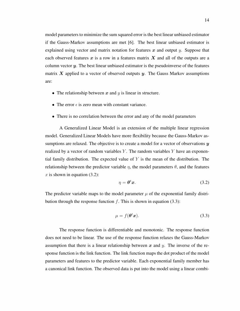
A Generalized Linear Model is an extension of the multiple linear regression

model. Generalized Linear Models have more flexibility because the Gauss-Markov as-

sumptions are relaxed. The objective is to create a model for a vector of observations y

realized by a vector of random variables Y . The random variables Y have an exponen-

tial family distribution. The expected value of Y is the mean of the distribution. The

relationship between the predictor variable η, the model parameters θ, and the features

x is shown in equation (3.2):

η = θtx. (3.2)

The predictor variable maps to the model parameter µ of the exponential family distri-

bution through the response function f . This is shown in equation (3.3):

µ = f(θtx). (3.3)

The response function is differentiable and monotonic. The response function

does not need to be linear. The use of the response function relaxes the Gauss-Markov

assumption that there is a linear relationship between x and y. The inverse of the re-

sponse function is the link function. The link function maps the dot product of the model

parameters and features to the predictor variable. Each exponential family member has

a canonical link function. The observed data is put into the model using a linear combi-

15

nation between the data and the model parameters. The objective of a GLM regression

is to estimate the GLM’s model parameters θ.

In linear regression the observed response is assumed to be normally distributed,

whereas in a GLM the observed response is from an exponential family distribution.

This is a relaxation of the Gauss-Markov assumption that the error is zero mean with

constant variance. In linear regression the response function is the identity function. The

GLM regression framework describes linear regression, logistic regression and Poisson

regression. In logistic regression the response function is the sigmoid function. A deeper

examination of GLMs can be found in [9].

An exponential family distribution is of the form shown in (3.4). The cumulant

ψ, also known as the log-partition function, is a normalizing function that ensures that

the integral over the exponential family distribution is one [11]:

p(x;θ) = h(x) exp(θtT (x)− ψ(θ)). (3.4)

The cumulant is a convex function. The cumulant also has the property that the

first derivative of the cumulant is the expected value of the distribution. The second

derivative is the covariance of the distribution. The T function is the sufficient statistic.

The sufficient statistic for the Bernoulli and multinomial distributions is the observed

datax. The h function is an artifact of the underlying measure of the probability function

[8]. It does not play a role in the PDLF model. The log likelihood for an exponential

family member is shown in equation (3.5) [2]:

l(θ;x) = θtT (x)− ψ(θ). (3.5)

3.3 Predictive Discrete Latent Factor Model

A PDLF model is used to estimate missing entries in a user-item matrix. This

problem is a fundamental problem in recommender systems. An accurate estimation

of a missing entry will lead to a better recommendation to a user. A PDLF model

returns a probability distribution for each entry or dyad. The probability distributions

are members of an exponential family. The probability distribution is used to make a

16

prediction about the value of the dyad.

The PDLF algorithm captures global structure and local structure through a gen-

eralized linear model (GLM). The term global structure is information across the whole

data set. Local structure is information with a cocluster. A cocluster is a cluster formed

from row and column clusters. A row clustering is a map from row number to a row

cluster. Similarly a column clustering is map from a column to a column cluster. The

coclusters are formed by both of these maps.

The coclustering algorithm assigns dyads to a cocluster by minimizing the mu-

tual information loss [7]. The algorithm intertwines the row and column clustering to

form coclusters. Dyads that have a high amount of mutual information are likely to be

assigned to the same cocluster. The coclustering algorithm is an NP hard problem. The

solution it produces is locally optimal [3].

A cocluster is associated with a single interaction effect referred to as δ. A dyad’s

interaction effect is referred to as δij . All of the interaction effects are referred to as ∆.

The row cluster assignments are ρ, which maps each row to a row cluster. The column

cluster assignments are γ, which maps each column to a column cluster.

The GLM determines an exponential family distribution for each dyad. The re-

gression coefficients β, capture information across the whole data set. If the exponential

family member is the Bernoulli distribution these coefficients are similar to the coeffi-

cients used in logistic regression. The interaction effects ∆, capture information shared

by different dyads within the same cocluster. The interaction effect δ is similar to the

bias term in logistic regression. The distinction is that there are as many interaction ef-

fects as there are coclusters. Instead of one bias term for all dyads, each dyad is assigned

to an interaction effect depending on its cocluster.

The regression coefficients and interaction effects are used to calculate the pre-

dictor variable η in the GLM. The predictor variable η is the regression coefficients

multiplied by the features and added to the interaction effects as shown in equation

(3.6). The response function maps the predictor variables to the exponential family dis-

tribution’s model parameters. This model shown in equation (3.6) is also known as the

random effects model [1]:

17

ηij = βtxij + δij. (3.6)

The regression coefficients β capture global structure. The interaction effects ∆

capture local structure. Each row and column is assigned to a row and column cluster.

Each dyad is assigned to a cocluster depending on its row and column. The interaction

effect’s value is determined by the dyad’s cocluster assignment. All dyads use the same

regression coefficients. The features for a dyad are xij .

The global and local structure is captured through a predictor variable in equation

(3.6). The predictor variable ηij maps to the model parameters of the exponential family

by a response function. The model parameters are used to create an exponential family

distribution for the dyad. Notice that the probability distribution will be different from

other dyads distributions based on its features xij and the interaction effect δij .

Notice the equation is similar to equation (3.1). The regression coefficients try to

capture the relationship between x and the output. The interaction effects try to capture

the error that the regression coefficients applied to the features and the true output. The

difference is that this uses a GLM framework and the interaction effects are determined

using a coclustering algorithm.

3.4 Fitting the PDLF Model

The hard clustering PDLF model is fitted by a generalized expectation maxi-

mization algorithm. The complexity is O(N(k + l)), where N is the number of known

dyads and k and l are the number of row and column clusters. The coclustering algo-

rithm requires that each known dyad is tested for membership in k + l coclusters. The

algorithm is specified in Algorithm 1. Note that this is the same algorithm as Algorithm

2 in [5], but some of the notation has been changed.

The expectation step assigns the dyads to row and column clusters. There are soft

clustering and hard clustering variants to the PDLF model. Except for the soft clustering

PDLF model with a multinomial distribution in Chapter 4, the experiments performed

for this thesis use the hard clustering variant. The coclusters are latent variables in the

model. The posterior probability is the probability of the cocluster conditioned on the

18

dyad and the model parameters β and ∆. The dyad is assigned to the cocluster where

this probability is the largest.

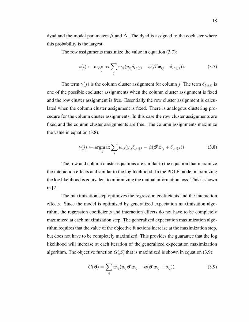
The row assignments maximize the value in equation (3.7):

ρ(i)← argmaxI

∑j

wij(yijδIγ(j) − ψ(βtxij + δIγ(j))). (3.7)

The term γ(j) is the column cluster assignment for column j. The term δIγ(j) is

one of the possible cocluster assignments when the column cluster assignment is fixed

and the row cluster assignment is free. Essentially the row cluster assignment is calcu-

lated when the column cluster assignment is fixed. There is analogous clustering pro-

cedure for the column cluster assignments. In this case the row cluster assignments are

fixed and the column cluster assignments are free. The column assignments maximize

the value in equation (3.8):

γ(j)← argmaxJ

∑i

wij(yijδρ(i)J − ψ(βtxij + δρ(i)J)). (3.8)

The row and column cluster equations are similar to the equation that maximize

the interaction effects and similar to the log likelihood. In the PDLF model maximizing

the log likelihood is equivalent to minimizing the mutual information loss. This is shown

in [2].

The maximization step optimizes the regression coefficients and the interaction

effects. Since the model is optimized by generalized expectation maximization algo-

rithm, the regression coefficients and interaction effects do not have to be completely

maximized at each maximization step. The generalized expectation maximization algo-

rithm requires that the value of the objective functions increase at the maximization step,

but does not have to be completely maximized. This provides the guarantee that the log

likelihood will increase at each iteration of the generalized expectation maximization

algorithm. The objective function G(β) that is maximized is shown in equation (3.9):

G(β) =∑ij

wij(yijβtxij − ψ(βtxij + δij)). (3.9)

19

The term ψ is the cumulant function of the exponential family member used in

the PDLF model. The objective function L(∆) that maximizes the interaction effects is

shown in equation (3.10):

L(∆) =∑ij

wij(yijδij − ψ(βtxij + δij)). (3.10)

The function takes the argument ∆ because all interaction effects are used if each co-

cluster has at least one dyad assigned to it. The weighting term wij ∈ {0, 1} represents

if there is a rating for the dyad ij.

Notice that both equation (3.9) and (3.10) are similar to the log likelihood in

equation (3.5). The difference is in the first term, which in the regression coefficients

equation excludes the interaction effects. Similarly, in the interaction effects equation,

the regression coefficients are excluded. In the hard clustering variant of the PDLF

model it is possible to combine the two equations to perform a GLM regression [5].

Maximizing the objective functions shown in equation (3.9) and (3.10) is the

same as maximizing the log likelihood. Recall the formula for log likelihood of an

exponential family member shown in equation (3.5). The regression coefficients and the

interaction effects are the model parameters θ shown in the log likelihood equation. For

some the Gaussian and Poisson exponential families there exists closed form solutions

that maximize equations (3.9) and (3.10). For the Bernoulli and multinomial models no

closed form solution exists. These maximizations are performed by numerical methods.

Suppose that θ is a vector with 37 elements, the maximization of the objective

function G(β) finds the regression coefficients that maximize G(β). These regression

coefficients are the first 36 elements in θ. The maximization of the L(∆) objective

function finds the interaction effect that maximizes L(∆). This interaction effect is the

last element in θ. Together the two objective functions maximize the log likelihood.

20

Algorithm 1 Hard PDLF AlgorithmInput: Response matrix Y ∈ R feature matrix X , weight matrix W , exponential familycumulant ψ, number of row clusters k, column clusters lOutput: Regression coefficients β, interaction effects ∆, row cluster assignments ρ,column cluster assignments γMethod: Initialize ρ and γ randomly. Choose good initializations for β and ∆.repeat

Generalized Expectation Step

Update row cluster assignments

ρ(i)← argmaxI

(∑j wij(yijδIγ(j) − ψ(βtxij + δIγ(j))

)Update column cluster assignments

γ(j)← argmaxJ(∑

iwij(yijδρ(i)J − ψ(βtxij + δρ(i)J)))

Generalized Maximization Step

Update interaction effects

δIJ ← argmaxδIJ

∑ij wij(yijδij − ψ(βtxij + δij))

Update regression coefficients

β ← argmaxβ∑

ij wij(yijβxij − ψ(βtxij + δij))

until convergencereturn (β,∆, ρ, γ)

Chapter 4

Using a Bernoulli as the Exponential

Family Member in a PDLF Model

4.1 Background

This chapter discusses the PDLF model that uses a Bernoulli distribution. It

verifies the results of the experiments in case study 1 [5]. It expands the experiments

by showing the model’s accuracy when using a different number of coclusters. It also

provides more detail on the implementation of the model. It compares the accuracy of

the PDLF model to the accuracy of the logistic model in Chapter 1.

4.2 Bernoulli Distribution

To use a Bernoulli distribution in a PDLF model the cumulant and the derivative

of the cumulant are needed. The derivative of the cumulant is used in the numerical

procedure that fits the model. The cumulant function for the Bernoulli distribution is

shown in (4.1):

ψ(θ) = log(1 + expθ). (4.1)

Note that the log function is the natural logarithm. The derivative of the Bernoulli cu-

mulant function is the sigmoid function. The canonical link function for a GLM that

21

22

uses a Bernoulli exponential family is shown in equation (4.2):

βtx = log

(θ

1− θ

). (4.2)

Recall that the response function is the inverse of the link function. The response

function for the Bernoulli exponential family is the sigmoid function which is shown in

equation (4.3):

θ =1

1 + exp−βtx. (4.3)

The notation describing the link and response function uses the regression coefficients.

This simplified notation is consistent with the literature on GLMs. The main purpose is

to state the link and the response functions. A more complete notation would include

the interaction effect. Notice that without the interaction effects this Bernoulli model is

fitted by logistic regression.

4.3 Optimization

The two optimization problems in the maximization step are concave optimiza-

tion problems. The cumulant function or log partition function is convex for all expo-

nential family members [11]. The negative of a convex function is a concave function.

The term before the cumulant function is an affine transformation. Convexity and con-

cavity are preserved under affine transformations. A nonnegative weighted sum of n

concave functions is also concave [4]. The concavity property provides guarantees that

finding a local optimum implies that a global optimum has been found. These optimiza-

tion problems are unconstrained which makes the optimization problem easier to solve.

Although these two optimization problems are convex, fitting the model is not. This is

due to the nonconvexity of the coclustering algorithm.

The maximization of the regression coefficients and interaction effects is per-

formed using gradient descent. At each iteration of the generalized expectation maxi-

mization algorithm, the parameters are optimized by performing three iterations of gra-

dient descent during the maximization step. The gradient of the regression coefficients

23

is shown in equation (4.4):

∂

∂βG(β) =

∑ij

wij(yijxij − ψ′(βtxij + δij)xij). (4.4)

The partial derivative of a single interaction effect is shown in (4.5):

∂

∂δL(∆) =

∑ij

wij(yij − ψ′(βtxij + δij)). (4.5)

The implementation uses up to five row clusters and five column clusters. The

new values for β and ∆ are set after both maximizations have completed. The row and

column assignments are set during the expectation step. There are five possible row

cluster assignments. The value for each row cluster assignment is computed and the

assignment that maximizes the function shown in equation (3.7). Similarly, the column

cluster assignments are computed by maximizing the function shown in (3.8).

There are implementation details which determine how the model parameters

are initialized. There are 459 different users so ρ is a column vector with 459 rows.

Each user is assigned at random to a row cluster. There are 1410 different movies so γ is

a column vector with 1410 rows. Each movie is assigned at random to a column cluster.

The regression coefficients β are initialized to a vector of zeros. The interaction effects

∆ are each initialized to 0.1.

4.4 Experiments

Five-fold cross-validation is performed on the same datasets used in the previous

logistic regression experiments. The algorithm is run five times, each time varying the

number of coclusters. The numbers of coclusters used are 25, 16, 9, 4, and 1. The same

number of row clusters is used as column clusters. Using only one cocluster should

capture the same information as performing logistic regression. The first case study in

Agarwal and Merugu’s paper [5] uses 25 coclusters. The average misclassification rate

for each number of coclusters is shown in Table 4.1. All of the plots in this section are

for the experiment that used 25 coclusters.

The algorithm runs for 50 iterations. At each iteration the state of β,∆, ρ and

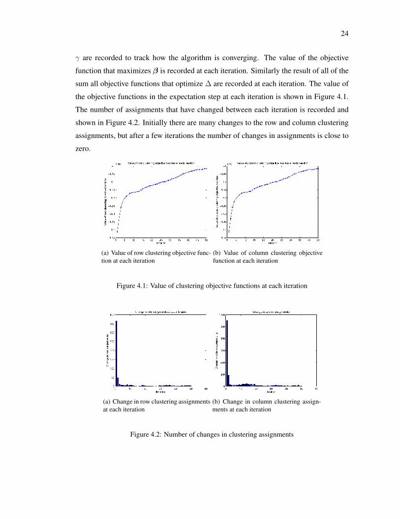
24

γ are recorded to track how the algorithm is converging. The value of the objective

function that maximizes β is recorded at each iteration. Similarly the result of all of the

sum all objective functions that optimize ∆ are recorded at each iteration. The value of

the objective functions in the expectation step at each iteration is shown in Figure 4.1.

The number of assignments that have changed between each iteration is recorded and

shown in Figure 4.2. Initially there are many changes to the row and column clustering

assignments, but after a few iterations the number of changes in assignments is close to

zero.

(a) Value of row clustering objective func-tion at each iteration

(b) Value of column clustering objectivefunction at each iteration

Figure 4.1: Value of clustering objective functions at each iteration

(a) Change in row clustering assignmentsat each iteration

(b) Change in column clustering assign-ments at each iteration

Figure 4.2: Number of changes in clustering assignments

25

Table 4.1: Misclassification rate using different number of coclusters

Coclusters Misclassification Std1 0.4219 0.00264 0.3168 0.00159 0.2993 0.001616 0.3016 0.001325 0.3004 0.0018

4.5 Analysis

The regression coefficients are shown in Figure 4.3. As expected the feature for

Drama has a large positive weight relative to other features. However the features for

War and Film-Noir are larger. Histograms of the Bernoulli parameter θ calculated for the

training data and testing data are in Figure 4.4. The similarity between the histograms

suggests that the trained model will be useful for predicting whether the rating will be a

four or a five.

Figure 4.3: Regression coefficients of the trained PDLF model

26

(a) Bernoulli parameter on training data (b) Bernoulli parameter on testing data

Figure 4.4: Training and testing Bernoulli parameters for one fold

The value of the objective functions is shown in Figure 4.5. The model parame-

ters and the likelihood versus iteration for one of the cross validation folds are plotted.

The log likelihood at each iteration is shown in Figure 4.5(c). The value of the objec-

tive function that maximizes the interaction effects ∆ increases at each iteration of the

algorithm. However the value of the objective function that maximizes the regression

coefficients β increases for the first two iterations then decreases. There exists a ten-

sion between optimizing both of these parameters. Initially the log likelihood of the

model is increased by optimizing the regression coefficients. After a few iteration the

number of dyads that change coclusters decreases. After the coclustering stabilizes the

log likelihood is increased more by optimizing the interaction effects. Although the two

objective functions maximize the log likelihood, the sum of the two objective functions

is not the log likelihood. Both objective functions subtract the value of the cumulant

function applied to the value of the predictor variable η. Therefore the difference be-

tween the sum of the two objective functions and the log likelihood is the value of the

cumulant function applied to the predictor variable η. In the hard clustering case it is

possible to combine the two objective functions into one objective function and use it to

perform the GLM regression [5].

The interaction effects are shown in Figure 4.6(b) in a Hinton diagram. The

blocks are red if the interaction effect is positive and the blue if the interaction effect is

negative. Notice that there are about nine coclusters that have most of the dyads. For

these nine coclusters notice that the absolute value of an interaction effect associated

27

(a) Value of objective function forregression coefficients

(b) Value of objective function forinteraction effects

(c) Log likelihood at each iteration

Figure 4.5: Values of the objective functions for the regression coefficients and interaction effectsand the log likelihood versus iteration

with the cocluster is larger for six of the nine coclusters. The three coclusters that have

a lot of dyads but small interaction effects contain dyads that can be estimated well

by using only the regression coefficients. Figure 4.6(a) has a Hinton diagram of the

cocluster assignments. The weight matrix for the Hinton diagram is number of dyads in

a training set that belong to each cocluster.

The Hinton diagram of cocluster membership shows that there are nine clusters

that have most of the assignments. This suggests that there are about nine different kinds

of coclusters in the data set. The model with nine coclusters had the lowest misclassifi-

cation rate of .2993. The difference in misclassification rate between the model with 25

and 9 coclusters is less than the standard deviation of the misclassification rate across

the folds. This means that using 9 coclusters will not consistently be more accurate.

However, using fewer coclusters will improve the runtime of the algorithm which is

O(N(k + l)). Recall that k + l is 6 if 3 row and 3 column clusters are used. It is 10

if 5 row and column clusters are used. If 3 row and column clusters are used then the

28

(a) Hinton diagram of cocluster as-signments

(b) Interaction effects

Figure 4.6: Hinton diagrams of cocluster assignments and interaction effects

runtime will be 60 percent of the runtime when 5 row and column clusters are used.

Decreasing the number of coclusters to four raised the misclassification rate to

0.3105. Finally only using one cocluster had a misclassification rate similar to using

logistic regression: 0.4219, whereas it is 0.4224 when performing logistic regression.

Notice that the misclassification rate is improved by 0.1114 by adding 3 coclusters.

Adding three parameters to a model and improving the misclassification by 26.4 percent

illustrates the power of the model.

The model with 25 coclusters has a misclassification rate of 0.3004 with a stan-

dard deviation of 0.0018. This is a better than 0.37 in the case study but the model

was trained on more examples. The model was better than a logistic regression model

which had a misclassification rate of 0.4220. A baseline classifier that always predicts

insignificant would have a misclassification rate of 0.4622.

Chapter 5

Using a Multinomial as the Exponential

Family Member in a PDLF Model

5.1 Background

I extend the PDLF model to use a multinomial as the exponential family mem-

ber. I evaluate the accuracy of the model when using only regression coefficients. Sim-

ilarly, the model’s accuracy is evaluated when using only interaction effects. I attempt

to improve the accuracy of the multinomial by using a soft clustering PDLF model, per-

forming annealing, and initializing the coclustering using sorting. The soft clustering

model does not improve accuracy. The soft clustering model’s accuracy suffers because

the dyads are spread uniformly across all coclusters. Essentially, the coclustering in the

soft clustering model is too soft to be useful. The model that uses annealing uses a mod-

ified hard coclustering algorithm presented in Algorithm 2. Annealing lowers the MSE,

but not by a significant amount. The variant that initializes the coclusters by sorting has

the lowers the MSE by a significant amount.

The response yij of the multinomial uses an indicator function which returns one

if the true outcome is the proposed outcome and zero otherwise. There are five possible

outcomes. Each outcome of the multinomial corresponds to a possible rating. The

algorithm generates a multinomial for each dyad. The expected value of the multinomial

is the predicted rating.

29

30

5.2 Using a GLM for a Multinomial distribution

In a GLM a predictor random variable η is a derived from a linear combination

of the predictor variables. The link function maps the predictor variable to the result

of the regression coefficients multiplied by the features. A GLM can use a vectorized

form. The feature weights and the interaction effects are mapped to the predictor random

variables by equation (5.1). The term k in equation (5.1) is an index to a single predictor

variable. The regression coefficients βtk and δk map to ηk according to (5.1):

ηk = βtkx+ δk. (5.1)

The term δ is a vector with five elements. The interaction effects contain a

scalar value for each class in the multinomial. The vectorized form of a GLM is useful

for distributions that have more than one parameter. For example a multinomial with n

outcomes has n− 1 parameters. Each parameter is the probability of a given outcome.

5.2.1 Algorithm Implementation

I use a five class multinomial because there are five different ratings. There are

five parameters for each feature. I use the first feature set with 36 features so β has

36 × 5 = 180 parameters. The implementation uses five row clusters and five column

clusters. However there are different interaction effects for each class, so there are

five interaction effects for each cocluster. Note that n in the cumulant function is the

number of classes which is five. The cumulant function ψ of the multinomial is shown

in equation (5.2):

ψ(η) = logn∑

k′=1

exp(ηk′). (5.2)

The cumulant can by shown to be convex by calculating the Hessian and applying the

Cauchy-Schwarz inequality [4]. The response function is the softmax function shown

in equation (5.3). The softmax function enforces the constraint that the sum of the

probabilities of each outcome is one. The response function maps the predictor variables

31

shown in equation (5.1) to the model parameters of the exponential family:

πk =exp(ηk)∑nk′=1 exp(ηk′)

. (5.3)

The multinomial has five model parameters πi each which give a probability of the

ith outcome. Essentially, the five class multinomial is constructed using five Bernoulli

models. Each Bernoulli model has a positive outcome if the rating corresponds to its

class otherwise the outcome is negative. It is helpful to think of this construction as a

one against all approach. The softmax function is used to generate the parameters of the

multinomial from the Bernoulli models.

5.2.2 Optimization

The optimization problems in the maximization step are adapted to use the multi-

nomial cumulant and response. I derive the gradients in this section. The regression

coefficients are chosen to maximize the objective function shown in equation (5.4):

G(β) =∑ij

wij

[5∑

k=1

I(yij, k)(βtkxij − ψ(βtxij + δij)

]. (5.4)

The equation is the same as equation (3.9), but the response and regression coefficients

are specific to the multinomial distribution. Notice the indicator function I which is

used to select the index k on the β. These are the regression coefficients associated with

the rating k. The response yij is the result of the indicator function which determines

whether the class k is the value of the rating. The feature parameters are optimized by

gradient descent. The derivation of the gradient is shown in Figure 5.1. For ease of

notation, I don’t use the weighting term wij . This derivation is similar to the derivation

of the gradient for the interaction effects.

The objective function used to optimize the interaction effects is similar to the

objective function in (3.10). As in the regression coefficients equation, the response

is specifically for the multinomial distribution. The interaction effects are chosen to

32

∂

∂βkG(β) =

∂

∂βk

[∑ij

I(yij, k)βtkxij − logn∑

k′=1

exp(ηk′)

]

=∂

∂βk

[∑ij

I(yij, k)βtkxij − logn∑

k′=1

exp(βtkxij + δk′)

]

=

[∑ij

xijI(yij, k)− 1∑nk′ exp(βtk′xij + δk′)

∂

∂βk

n∑k′

exp(βtk′xij + δk′)

]

=

[∑ij

xijI(yij, k)− exp(βtkxij + δk)∑nk′ exp(βtk′xij + δk′)

∂

∂βk

[βtkxij + δk

]]

=

[∑ij

xijI(yij, k)− exp(βtkxij + δk)∑nk′ exp(βtk′xij + δk′)

xij

]

Figure 5.1: Derivation of the gradient for the regression coefficients

maximize the objective function shown in (5.5):

L(∆) =∑ij

wij

5∑k=1

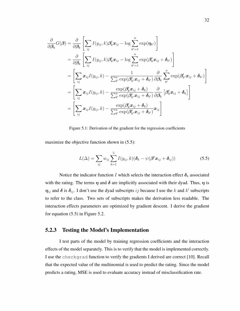
I(yij, k)(δk − ψ(βtxij + δij)) (5.5)

Notice the indicator function I which selects the interaction effect δk associated

with the rating. The terms η and δ are implicitly associated with their dyad. Thus, η is

ηij and δ is δij . I don’t use the dyad subscripts ij because I use the k and k′ subscripts

to refer to the class. Two sets of subscripts makes the derivation less readable. The

interaction effects parameters are optimized by gradient descent. I derive the gradient

for equation (5.5) in Figure 5.2.

5.2.3 Testing the Model’s Implementation

I test parts of the model by training regression coefficients and the interaction

effects of the model separately. This is to verify that the model is implemented correctly.

I use the checkgrad function to verify the gradients I derived are correct [10]. Recall

that the expected value of the multinomial is used to predict the rating. Since the model

predicts a rating, MSE is used to evaluate accuracy instead of misclassification rate.

33

∂

∂δkL(∆) =

∂

∂δk

[∑ij

I(yij, k)δk − logn∑

k′=1

exp(ηk′)

]

=∂

∂δk

[∑ij

I(yij, k)δk − logn∑

k′=1

exp(βtk′xij + δk′)

]

=∑ij

I(yij, k)− 1∑nk′=1 exp(βtk′xij + δk′)

∂

∂δk

n∑k′=1

exp(βtk′xij + δk′)

=∑ij

I(yij, k)− exp(βtkxij + δk)∑nk′=1 exp(βtk′xij + δk′)

Figure 5.2: Derivation of the gradient for the interaction effects

The checkgrad function shows that the gradients are computed correctly. The

model was tested for 50 iteration with a learning rate of 10−5. During an iteration of the

generalized expectation maximization algorithm the regression coefficients and interac-

tion effects are optimized by three iterations of gradient descent. I use gradient descent

not stochastic gradient descent for all of the optimizations of the PDLF multinomial

model. Stochastic gradient descent is more efficient, but I found gradient descent a little

bit easier to implement and check with the checkgrad function.

5.3 Testing the Regression Coefficients

The model is tested without using the interaction effects. The regression coef-

ficients are initially set to zero. Equation (5.4) is maximized by gradient descent. The

generalized expectation maximization algorithm trains the model for 50 iterations. The

regression coefficients are optimized by three iterations of gradient descent for each iter-

ation of the generalized expectation maximization algorithm. The value of the objective

function in equation (5.4) at each iteration is shown in Figure 5.3(a). Since there is

no coclustering the model is optimized by multinomial logistic regression. The opti-

mization problem is a concave maximization problem and it appears to converge to the

maximum.

34

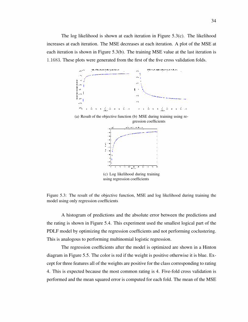
The log likelihood is shown at each iteration in Figure 5.3(c). The likelihood

increases at each iteration. The MSE decreases at each iteration. A plot of the MSE at

each iteration is shown in Figure 5.3(b). The training MSE value at the last iteration is

1.1683. These plots were generated from the first of the five cross validation folds.

(a) Result of the objective function (b) MSE during training using re-gression coefficients

(c) Log likelihood during trainingusing regression coefficients

Figure 5.3: The result of the objective function, MSE and log likelihood during training themodel using only regression coefficients

A histogram of predictions and the absolute error between the predictions and

the rating is shown in Figure 5.4. This experiment used the smallest logical part of the

PDLF model by optimizing the regression coefficients and not performing coclustering.

This is analogous to performing multinomial logistic regression.

The regression coefficients after the model is optimized are shown in a Hinton

diagram in Figure 5.5. The color is red if the weight is positive otherwise it is blue. Ex-

cept for three features all of the weights are positive for the class corresponding to rating

4. This is expected because the most common rating is 4. Five-fold cross validation is

performed and the mean squared error is computed for each fold. The mean of the MSE

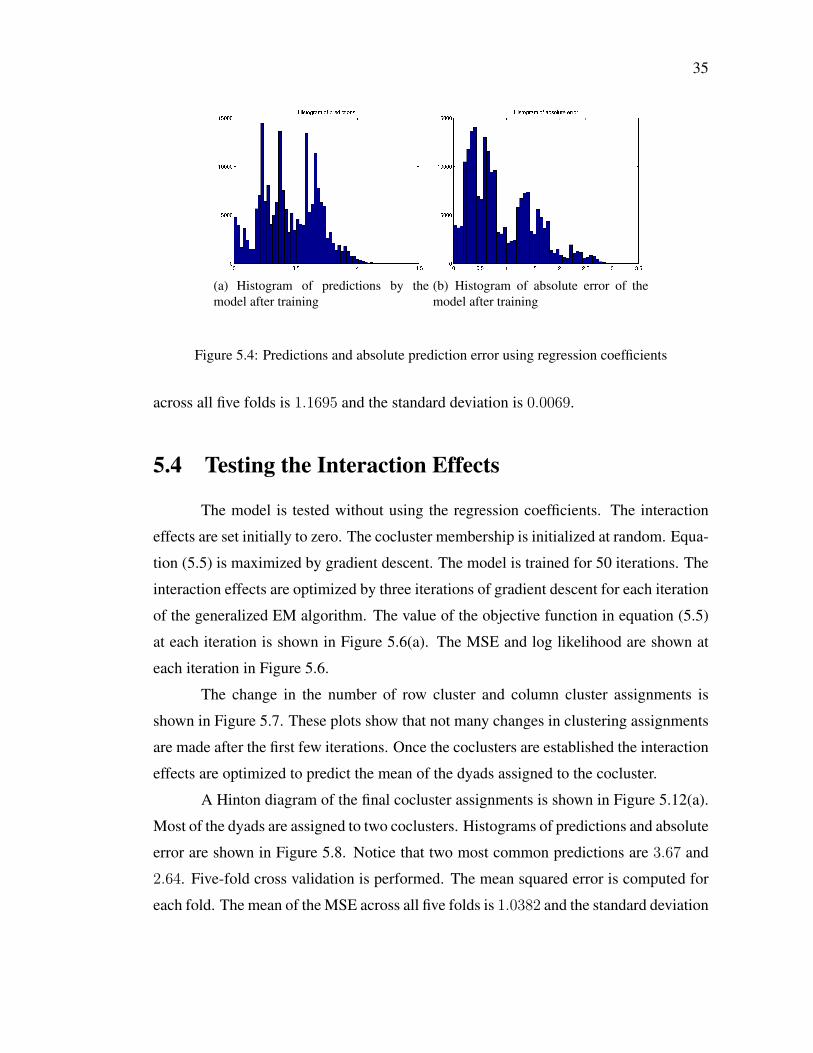
35

(a) Histogram of predictions by themodel after training

(b) Histogram of absolute error of themodel after training

Figure 5.4: Predictions and absolute prediction error using regression coefficients

across all five folds is 1.1695 and the standard deviation is 0.0069.

5.4 Testing the Interaction Effects

The model is tested without using the regression coefficients. The interaction

effects are set initially to zero. The cocluster membership is initialized at random. Equa-

tion (5.5) is maximized by gradient descent. The model is trained for 50 iterations. The

interaction effects are optimized by three iterations of gradient descent for each iteration

of the generalized EM algorithm. The value of the objective function in equation (5.5)

at each iteration is shown in Figure 5.6(a). The MSE and log likelihood are shown at

each iteration in Figure 5.6.

The change in the number of row cluster and column cluster assignments is

shown in Figure 5.7. These plots show that not many changes in clustering assignments

are made after the first few iterations. Once the coclusters are established the interaction

effects are optimized to predict the mean of the dyads assigned to the cocluster.

A Hinton diagram of the final cocluster assignments is shown in Figure 5.12(a).

Most of the dyads are assigned to two coclusters. Histograms of predictions and absolute

error are shown in Figure 5.8. Notice that two most common predictions are 3.67 and

2.64. Five-fold cross validation is performed. The mean squared error is computed for

each fold. The mean of the MSE across all five folds is 1.0382 and the standard deviation

36

Figure 5.5: Regression coefficients

is 0.0060.

5.5 Testing the multinomial PDLF model

The optimization of the model parameters is as follows. During one iteration

of the generalized expectation maximization algorithm, the regression coefficients are

optimized, then the interaction effects are optimized, then coclustering is performed.

At each iteration of the generalized expectation maximization algorithm the regression

coefficients are optimized by three iterations of gradient descent. The previous vector

of regression coefficients is kept for the optimization of the interaction effects. The

interaction effects are optimized by three iterations of gradient descent. The newly

optimized regression coefficients and interaction effects are used in the coclustering

steps.

The coclustering steps consist of performing row clustering and column clus-

tering. Row clustering is performed first, followed by column clustering. The row and

37

(a) Result of the objective func-tion

(b) MSE during training usinginteraction effects

(c) Log likelihood during train-ing using interaction effects

Figure 5.6: The result of the objective function, MSE, and log likelihood during training themodel using only interaction effects

(a) Change in row assignments using in-teraction effects

(b) Change in column assignments usinginteraction effects

Figure 5.7: Change in coclustering assignments using interaction effects

column clustering is done by performing calculations shown in equations (3.7) and (3.8)

for each possible row and column assignment. The assignments are made after the row

and column calculations have finished by applying the argmax operator. The full model

is trained for 50 iterations. The model parameters are initialized to zero. The rows and

columns are initially assigned to row and column clusters at random.

The log likelihood, the value of the objective functions in equations (5.4) and

(5.5) is shown at each iteration are shown in Figure 5.9. The log likelihood increases

at each iteration. The plots of the objective functions are similar to the plots in Figures

4.5(a) and 4.5(b) which plot the objective functions of the PDLF model that uses a

Bernoulli distribution. For the first few iterations the regression coefficients have a

38

(a) Histogram of predictions (b) Histogram of absolute error

Figure 5.8: Histogram of predictions and absolute error using interaction effects

greater effect on the log likelihood than the interaction effects. When the assignment of

the coclusters stabilizes the interaction effects have a greater effect than the regression

coefficients.

Histograms of predictions and the absolute error are shown in Figure 5.10. The

predictions seem to be bimodal. The two groups of predictions are between 3.5 and 4,

and between 2.5 and 3. This is expected because there are two coclusters that contain

most of the dyads.

The final model parameters of the regression coefficients and the interaction ef-

fects are shown in Figure 5.11. Eleven of the of the weights are negative for the class

corresponding to rating 4. Recall that the model that only used regression coefficients

had 3 negative weights for the class that corresponding to rating 4. This is expected

because the interaction effects have been introduced to affect the predictions. Notice

that there are five different interaction effects that are captured. There are five coclus-

ters each of which bias the prediction towards one of the five ratings. The cocluster

assignments after training are shown in Figure 5.12(b). The number of changes in row

and column cluster assignments at each iteration is shown in Figure 5.13(a) and 5.13(b).

The cocluster which contains the most dyads biases the prediction to the most common

rating four. This limits the amount of information the model can capture and lowers the

MSE. The MSE is evaluated using five-fold cross validation. The mean squared error

is computed for each fold. The mean of the MSE across all five folds is 1.0062 and the

standard deviation is 0.0190.

39

(a) Value of the regression coeffi-cients objective function

(b) Value of the interaction effectsobjective function

(c) Log likelihood during trainingof PDLF Algorithm

Figure 5.9: MSE and log likelihood during training of the hard clustering PDLF model

5.5.1 Annealing to improve coclustering

I modified the coclustering assignment to perform annealing. The model still

uses hard clustering because each dyad belongs to only one cocluster. Recall the original

clustering assignment is done by performing an argmax over equations (3.7) and (3.8).

I compute probabilities that each row and column belong to a row cluster and column

cluster. These probabilities form a multinomial distribution. I sample the multinomial

distribution and the outcome is the row or column assignment.

Recall that the row clustering equation (3.7) performs an argmax over the equa-

tion. To perform annealing I use the values in equation (5.6):

vi =∑j

wij(yijδiγ(j) − ψ(βtxij + δij)). (5.6)

to compute probabilities. The values for each cluster assignment in equations and can

be negative or positive. I use the softmax to transform these values into well calibrated

40

(a) Histogram of predictions of thetrained model

(b) Histogram of the absolute error be-tween predictions and ratings

Figure 5.10: Histogram of predictions and absolute error on training data

(a) Regression coefficients (b) Interaction effects

Figure 5.11: Hinton diagrams of regression coefficients and interaction effects of the hard clus-tering PDLF model

probabilities. These probabilities are parameters to the multinomial that is sampled.

An analogous procedure for the column clustering. I use this cocluster assignment for

the first 25 iterations of the generalized EM algorithm. The last 25 iterations I use

the original coclustering assignment. The coclustering algorithm that uses annealing is

presented in Algorithm 2.

Using annealing slightly lowers the MSE. The change in the number of row

and column cluster assignments is shown in Figures 5.14(a) and 5.14(b). There are

more changes to row and column cluster membership in the first five iterations when

annealing is used. The final cocluster assignments are shown in a Hinton diagram in

Figure 5.12(c). Unfortunately, annealing does not seem to distribute the dyads across

41

(a) Hinton diagram of coclus-tering assignments using inter-action effects

(b) Cocluster membership of apdlf model

(c) Cocluster membershipwhen using annealing

Figure 5.12: Coclustering assignments using different variations of the coclustering algorithmor pdlf model

more coclusters. The accuracy of the models is determined by using five-fold cross

validation. The mean MSE across all five folds is 1.0014 with a standard deviation of

0.0118.

Algorithm 2 Row clustering algorithm that uses annealingT ← EM iterationsfor t = 1 to T do

if t ≤ T2

thenfor k = 1 to m dovk ←

∑j wij(yijδiγ(j) − ψ(βtxij + δiγ(j)))

end forfor k = 1 to m doπk ←

exp(vk)∑mk′=1 exp(vk′)

end forρ(i)← Sample(Multinomial(π))

elseρ(i)← argmax

kv

end ifend for

5.5.2 Soft clustering approach

A clustering algorithm that uses soft clustering or annealing may spread the

dyads across more coclusters. The hard clustering model’s accuracy suffers from over-

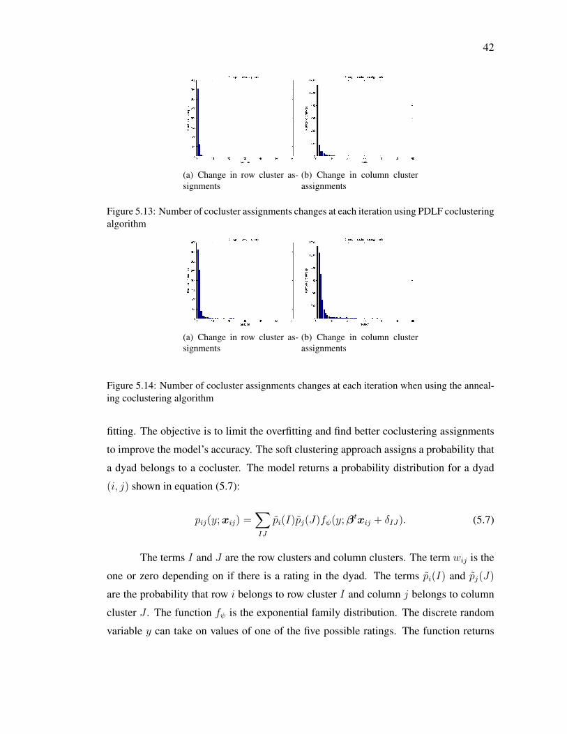
42

(a) Change in row cluster as-signments

(b) Change in column clusterassignments

Figure 5.13: Number of cocluster assignments changes at each iteration using PDLF coclusteringalgorithm

(a) Change in row cluster as-signments

(b) Change in column clusterassignments

Figure 5.14: Number of cocluster assignments changes at each iteration when using the anneal-ing coclustering algorithm

fitting. The objective is to limit the overfitting and find better coclustering assignments

to improve the model’s accuracy. The soft clustering approach assigns a probability that

a dyad belongs to a cocluster. The model returns a probability distribution for a dyad

(i, j) shown in equation (5.7):

pij(y;xij) =∑IJ

pi(I)pj(J)fψ(y;βtxij + δIJ). (5.7)

The terms I and J are the row clusters and column clusters. The term wij is the

one or zero depending on if there is a rating in the dyad. The terms pi(I) and pj(J)

are the probability that row i belongs to row cluster I and column j belongs to column

cluster J . The function fψ is the exponential family distribution. The discrete random

variable y can take on values of one of the five possible ratings. The function returns

43

a probability distribution when the exponential family member is parameterized by the

regression coefficients and interaction effects.

The maximization step in the soft clustering models maximizes the regression

coefficients, interaction effects, and mixture component priors. The mixture component

priors are the prior probabilities that a dyad is assigned to a cocluster. The mixture

component priors are calculated using equation (5.8):

πIJ =1

N

∑ij

wij pi(I)pj(J). (5.8)

Note thatN is the number of known entries, and it is calculated by using equation

(5.9):

N =∑ij

wij. (5.9)

The optimization of the regression coefficients includes the cocluster membership prob-

abilities when using the soft clustering PDLF model. Essentially this is the weighted

sum of the objective functions in the hard clustering model. Note that there is a different

interaction effect used for each cocluster. The weights are the probability that the dyad

belongs to the cocluster, which is pi(I)pj(J). The regression coefficients are optimized

using equation (5.10):

G(β) =∑ij

wij∑IJ

pi(I)pj(J)(yijβtxij − ψ(βtxij + δIJ)). (5.10)

The optimization of the interaction effects is extended to use the soft cluster-

ing model. This is the weighted sum of the objective function in the hard clustering

model. However, instead of one interaction effect, the interaction effect associated with

the current cocluster is used. The amount is weighted by the probability that the dyad

belongs to the cocluster. This is similar to how the objective function that optimizes the

regression coefficients. The interaction effects are optimized using equation (5.11):

L(∆) =∑ij

wij∑IJ

pi(I)pj(J)(yijδIJ − ψ(βtxij + δIJ)). (5.11)

The expectation step of the generalized expectation maximization algorithm in-

44

volves calculating the row and column cluster membership probabilities. The term wi is

number of all known entries in the row. The term ci is a normalizing factor to guarantee

that sum of p(i) across all row clusters is one. The probability that a row i is assigned to

a cocluster is shown in equation (5.12):

pi(I)← ci

(∏j,J

(πIJfψ(yij;βtxij + δIJ)wij pj(J)

) 1wi

. (5.12)

Although the notation is complicated it is easy to see how it is possible to cause

numerical underflow when running the soft clustering algorithm on a dataset that has a

few hundred entries in each row. Notice that πIJ and fψ are two probabilities multiplied

together. This value increases when it is exponentiated by a probability. Numerical

underflow may occur when performing the product of all of these values. Numerical

underflow can be avoided by taking the log of soft clustering equation. The log of the

soft row clustering assignment equation is shown in equation (5.13).

log pi(I) =1

wi

∑j

wij∑J

pj(J) log πij + pj(J) log fψ(yij;βtxij + δIJ). (5.13)

Equation (5.13) will return a negative number which will be associated with the

row cluster membership. These values are mapped to probabilities using the softmax

function. The softmax function plays the role of the ci term in equation (5.12). This

term is used to normalize the values to well calibrated probabilities. The calculation of

the column cluster membership probabilities is similar to the row cluster membership

probability calculation. The probability that a column j is assigned to a cocluster is

shown in (5.14).

pj(J)← ci

(∏i,I

(πIJfψ(yij;βtxij + δIJ)wij pi(I)

) 1wj

. (5.14)

I implement the soft clustering PDLF model. I initialized the row and column

cluster membership probabilities randomly using Matlab’s rand function. I initialize

the interaction effects randomly using Matlab’s rand function. The generalized expec-

45

tation maximization algorithm is run for 50 iterations. At each iteration the gradient

descent is performed three times to optimize the regression coefficients and interaction

effects.

5.5.3 Analysis of the soft clustering model

The model is trained correctly but it assigns each dyad uniformly to all of the

coclusters. I verified that the model is implemented correctly by checking the gradients

using Matlab’s checkgrad function, calculating the log likelihood and the MSE dur-

ing training. The log likelihood increases while the MSE decreases as shown in Figure

5.15.

I tried different initializations of the row and column cluster distributions and

interaction effects. If I initialize the row and column cluster distributions uniformly, they

stay uniform. If I initialize the interaction effects to zero and the row and column cluster

distributions uniformly, the interaction effects will be the same at each iteration of the

algorithm. The row and column cluster distributions will remain uniform throughout

the algorithm. If I initialize the interaction effects to have some coclusters bias towards

certain ratings, the row and column cluster distributions will eventually become uniform.

I believe the model is implemented correctly because the likelihood increases. I believe

that the model is being fitted properly because I have verified that the gradients are

correct. This PDLF multinomial model may not benefit from soft coclustering. It may

be that the way to maximize the likelihood in this model is to cocluster uniformly for all

of the dyads.

The mixture components of the fitted soft clustering PDLF model are shown

in Figure 5.16(a). The interaction effects of the fitted soft clustering PDLF model are

shown in Figure 5.16(b). The mixture components probabilities are uniform because

the row and column cluster probabilities are uniform. This means that each dyad has

the same membership probability for each cocluster. Hence, each dyad is essentially

assigned only one interaction effect. In the soft clustering case when using a multinomial

the PDLF model lack of effective coclustering makes the model as accurate as a PDLF

model with only one cocluster.

I perform five-fold cross validation to test the soft clustering PDLF model. The

46

(a) MSE during training of thesoft clustering PDLF model

(b) Log likelihood during train-ing of the soft clustering PDLFmodel

Figure 5.15: MSE and log likelihood during training of the soft clustering PDLF model

mean MSE across the five folds is 1.1559 and the standard deviation is 0.0065. Notice

that this MSE is marginally better than using a PDLF model with only the regression

coefficients.

(a) Mixture component priors (b) Interaction effects in thesoft clustering PDLF model

Figure 5.16: Mixture component priors and interaction effects of the soft clustering PDLF model

5.5.4 Cocluster initialization by sorting

Previous variations of the multinomial model inialize the coclusters at random.

This variation the row and columns are initially clustered by the mean rating for each

row or column. The mean rating of a row is a user’s mean rating. The mean rating of the

column is the mean rating of the movie. The goal is to find more informative clusters

instead of one or two coclusters that contain most of the dyads.

Recall that a cocluster captures the average rating of the dyads assigned to the

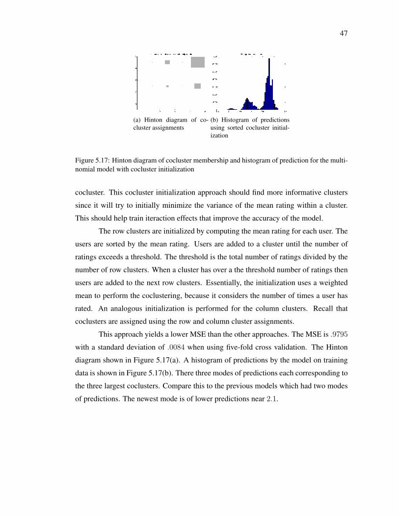
47

(a) Hinton diagram of co-cluster assignments

(b) Histogram of predictionsusing sorted cocluster initial-ization

Figure 5.17: Hinton diagram of cocluster membership and histogram of prediction for the multi-nomial model with cocluster initialization

cocluster. This cocluster initialization approach should find more informative clusters

since it will try to initially minimize the variance of the mean rating within a cluster.

This should help train iteraction effects that improve the accuracy of the model.

The row clusters are initialized by computing the mean rating for each user. The

users are sorted by the mean rating. Users are added to a cluster until the number of

ratings exceeds a threshold. The threshold is the total number of ratings divided by the

number of row clusters. When a cluster has over a the threshold number of ratings then

users are added to the next row clusters. Essentially, the initialization uses a weighted

mean to perform the coclustering, because it considers the number of times a user has

rated. An analogous initialization is performed for the column clusters. Recall that

coclusters are assigned using the row and column cluster assignments.

This approach yields a lower MSE than the other approaches. The MSE is .9795

with a standard deviation of .0084 when using five-fold cross validation. The Hinton

diagram shown in Figure 5.17(a). A histogram of predictions by the model on training

data is shown in Figure 5.17(b). There three modes of predictions each corresponding to

the three largest coclusters. Compare this to the previous models which had two modes

of predictions. The newest mode is of lower predictions near 2.1.

48

Table 5.1: Zero/One misclassification rates for the multinomial models

Model Misclassification StdStandard 0.3512 0.0158Sorted 0.3356 0.003

5.6 Comparison between the Bernoulli and multinomial

models

I evaluate the zero/one misclassification of the multinomial models to provide a

comparison against the Bernoulli models. A training example is correctly classified if

the rating is greater than the mean and the model predicts a rating greater than the mean.

Similarly a training example is correctly classified if the rating is less than the mean

and the model predicts a rating less than the mean. The standard multinomial model is

the variant that initializes the coclusters at random and does not use soft clustering or

annealing. The standard multinomial model and the multinomial model that uses sorting

in the initialization of the coclusters are compared against the Bernoulli models.

The mean movie rating is 3.5009. The mean misclassification and standard devi-

ation is shown in Table 5.1. The misclassification rate is greater than the misclassifica-

tion rate in the Bernoulli models. The multinomial model that initializes the coclusters

by sorting has a better zero/one accuracy than the multinomial that initializes its coclus-

ters at random. Recall that the Bernoulli model with the lowest misclassification rate

had a misclassification rate of 0.2993.

It is expected that the multinomial PDLF model does not perform as well as

the Bernoulli PDLF model. The multinomial distribution is created by training five

Bernoulli distributions. Recall that each Bernoulli had a positive outcome if the rating

corresponded to its class and a negative outcome otherwise. The PDLF model that used

a Bernoulli had a positive outcome if the rating is 4 or 5 and negative otherwise. It may

be easier to train a Bernoulli to distinguish ratings of 4 and 5 from ratings 1,2, and 3.

Chapter 6

Conclusions

The accuracy of the PDLF model with a Bernoulli distribution shows the power

of the PDLF model. The model worked well because the coclustering component of

the PDLF model was able to discover local structure within the data. The model used

the same features as the logistic regression models. However the difference in accuracy

may be lessened if better features were selected for the logistic regression model and

regularization was used.

The weak performance of the multinomial model is because the coclustering is

not able to find as much local structure within the data. The accuracy may be improved

by first using the soft clustering model for a few iterations then using the hard clustering

model. This is similar to using annealing. The soft clustering approach would find a

good starting point to perform hard clustering.

Another approach would be to use ordinal regression. A multinomial is for nom-

inal data. Movie ratings are categorical data because there is an order to the ratings. A

variant of ordinal regression uses a probit model. Under a probit ordinal regression

framework it may be possible to use a PDLF model. In this case the exponential family

member would be a Normal distribution.

49

Bibliography

[1] Alan Agresti. Categorical Data Analysis. Wiley-Interscience, second edition,2002.

[2] Inderjit Dhillon Joydeep Ghosh Arindam Banerjee, Srujana Merugu. Clusteringwith bregman divergences. JMLR, 2005.

[3] Joydeep Ghosh Srujana Merugu Dharmendra S. Modha Arindam Banerjee, Inder-jit Dhillon. A generalized maximum entropy approach to bregman co-clusteringand matrix approximation. JMLR, 2007.

[4] S. Boyd and L. Vandenberghe. Convex Optimization. Cambridge University Press,first edition, 2004.

[5] Srujana Merugu Deepak Agarawal. Predictive discrete latent factor models forlarge scale dyadic data. KDD, 2007.

[6] Jeff Gill. Generalized Linear Models A Unified Approach. Sage PublicationsLimited, first edition, 2000.

[7] D. Hodha I. Dhillon, S. Mallela. Information-theoretic co-clustering. KDD, 2003.

[8] Michael Jordan. Notes on The exponential family and generalized linear models.

[9] P. McCullagh and J.A Nelder. Generalized Linear Models. Chapman and Hall,second edition, 1989.

[10] Carl Rassmussen.http://www.kyb.tuebingen.mpg.de/bs/people/carl/code/minimize/checkgrad.m.

[11] Alex Smola.http://videolectures.net/mlss06au smola ef/.

50